prediction of the axisymmetric impinging jet with ...lada/postscript_files/aldo_thesis.pdf · in...

THESIS FOR THE DEGREE OF MASTER OF SCIENCE

Prediction of the AxisymmetricImpinging Jet with Different� � �

Turbulence Models

ALDO GERMAN BENAVIDES MORAN

Department of Thermo and Fluid Dynamics

CHALMERS UNIVERSITY OF TECHNOLOGY

Goteborg, Sweden 2004

Prediction of the Axisymmetric Impinging Jet with Different ��Turbulence ModelsALDO GERMAN BENAVIDES MORAN

c�

ALDO GERMAN BENAVIDES MORAN, 2004

Diploma Work 04/29

Institutionen for termo- och fluiddynamikChalmers Tekniska HogskolaSE-412 96 Goteborg, SwedenPhone +46-(0)31-7721400Fax: +46-(0)31-180976

Printed at Chalmers ReproserviceGoteborg, Sweden 2004

Prediction of the Axisymmetric Impinging Jetwith Different �� Turbulence Models

by

Aldo German Benavides [email protected]

Department of Thermo and Fluid DynamicsChalmers University of Technology

SE-412 96 GoteborgSweden

AbstractThe present work focuses on studying the axisymmetric turbulent im-pinging jet numerically. A low-Reynolds �� model and the wall-normalReynolds stress elliptic relaxation turbulence model ( �� model) areimplemented in an in-house Navier-Stokes solver to accomplish the com-putations. In the present case, the inlet is located two diameters abovethe impingement wall; the Reynolds number is �� and the flowbeing fully developed at the jet discharge. The different results are com-pared with existing experimental data for their validation.

The standard �� model fails in predicting flow fields where a stag-nation point is encountered and/or strong streamline curvature takesplace. This is the case of the impinging flow which is dominated by ir-rotational straining and flow curvature. Due to its high heat transferrates near the stagnation point, impinging jets have been used in manyengineering and industrial applications where heating or cooling pro-cesses are required. Hence the necessity of developing improved turbu-lence models which let us correctly forecast the flow and thermal fieldsof this type.

The �� model is found to perform much better than ordinary two-equation closure models for this flow configuration. As a consequence anew time scale constraint, based on the realizable � �� model, is im-plemented for the low-Reynolds � �!� model. This time scale constraintsubstantially improves the flow predictions near the stagnation pointand in the wall-jet region, as well as a better heat transfer coefficientis obtained. Finally, the use of a limiter for the production of kineticenergy in the low-Reynolds �"�!� model is also examined.

iii

Acknowledgments

I would like to express my sincere thanks to Professor Lars Davidson,my supervisor, for his guidance and support throughout the course ofthis project. The many discussions I have had with him have benefittedconsiderably my understanding of Computational Fluid Dynamics(CFD) and turbulence modelling.

Understanding the code and clearing up the problems which sometimescame out was just not possible without the help and expertise of A. Sven-ingsson.

I have greatly enjoyed every single day of the last eighteen monthsstudying in Chalmers and living in Sweden. I would like to thank every-one taking part in the Master’s programme in Turbulence, specially toProfessor W.K. George & Docent Gunnar Johansson for their constantsupport, advice and kindness no matter how busy they were. I havealways been very proud of having the opportunity to participate in thisextraordinary programme and I can say with no doubt it was one of thebest experiences of my life, so far.

I specially thank my family for their support during my stay in Sweden.Without their help and encouragement nothing would have been possi-ble.

Last, but by no means least, I would like to thank everyone at the De-partment, for making such a pleasant and work friendly atmosphere.Being part of TFD is wonderful!

v

Contents

Abstract iii

Acknowledgments v

1 Introduction 11.1 Relevant past studies . . . . . . . . . . . . . . . . . . . . . . 11.2 Experimental test case for validation . . . . . . . . . . . . . 3

2 Governing Equations 5

3 Turbulence Models Considered 93.1 Low-Reynolds-Number � �!� Model . . . . . . . . . . . . . . 93.2 Standard � � � Model . . . . . . . . . . . . . . . . . . . . . 103.3 Realizable � � � Model . . . . . . . . . . . . . . . . . . . . . 123.4 Time Scale Constraint for Low-Reynolds-

Number Model . . . . . . . . . . . . . . . . . . . . . . . . . . 143.5 Limiter for

��in Low-Reynolds-Number

Model . . . . . . . . . . . . . . . . . . . . . . . . . . . . . . . 143.6 Turbulent heat flux . . . . . . . . . . . . . . . . . . . . . . . 15

4 Computational Approach 174.1 The Solver . . . . . . . . . . . . . . . . . . . . . . . . . . . . 174.2 Axisymmetry considerations . . . . . . . . . . . . . . . . . . 174.3 Numerical Method . . . . . . . . . . . . . . . . . . . . . . . 194.4 Domain and Boundary Conditions . . . . . . . . . . . . . . 20

5 Results and Discussion 255.1 Performance of the Time Scale Constraint . . . . . . . . . . 255.2 Limiter effect on the AKN model . . . . . . . . . . . . . . . 315.3 Comparison of the results given by the Constraint and the

Limiter . . . . . . . . . . . . . . . . . . . . . . . . . . . . . . 325.3.1 Near-wall behavior . . . . . . . . . . . . . . . . . . . 355.3.2 Time-Scale Constraint and Limiter operation . . . . 37

5.4 Heat transfer coefficient . . . . . . . . . . . . . . . . . . . . 39

6 Future Work 45

vii

Chapter 1

Introduction

The axisymmetric impinging jet studied in this work is a typical exam-ple of wall-bounded shear flows. The inlet flow which is fully developedexits a pipe of diameter � at a height of � jet diameters from the wall( �� ), impinges onto the wall surface and disseminates radiallyalong the solid boundary. Due to its high level of heat transfer ratenear the stagnation point, jet impingement is used in many engineeringand industrial applications where heating, cooling or drying processesare required. Examples of such applications are cooling of gas turbineblades and electronic equipment.

The flow field of an impinging jet comprises three distinctive flow re-gions, namely a free jet region, a deflection region (or stagnation region)and a wall jet region as shown in Figure 1.1. A shear layer is createddue to the velocity difference between the potential core of the jet andthe ambient fluid. Commonly this shear layer is the source of the tur-bulence in the jet, however as the inlet-to-wall distance is so short inthe present case, there is not enough gap for mixing to happen withthe surrounding fluid. As a result, the flow field in the vicinity of thestagnation point has a low turbulence intensity.

In the free jet region, the mean shear strain is zero and the pro-duction of kinetic energy is exclusively due to the normal straining. Asthe flow approaches the wall, the centerline velocity decreases to zeroat the stagnation point. Moreover, the proximity of the solid boundarycauses the deflection of the jet and a strong streamline curvature regionis observed. Downstream the stagnation point, a wall jet evolves alongthe wall. Turbulence energy is increased due to the mean shear strainwhich dominates in the near-wall region.

1.1 Relevant past studies

All the flow characteristics described above make the axisymmetric im-pinging jet a challenging case for turbulence models. Previous numer-ical computations revealed the lack of accuracy of some models in pre-

1

Prediction of the Axisymmetric Impinging Jet with Different �� TurbulenceModels

�

�

��

�

��

potential core

wall jet region

deflection region

free jet region

Figure 1.1: Flow regions of an axisymmetric impinging jet

dicting the turbulent quantities near the stagnation point. As an exam-ple, the standard � �"� model overestimates the turbulent kinetic energyin the deflection region, leading to extremely high values of the com-puted heat transfer coefficient. Numerous computations with differentconfigurations of impinging jets have been carried out, showing that theRANS (Reynolds-Averaged Navier-Stokes equations) models performreasonably well in most of the flow domain. However, the stagnationand near-wall regions are not properly resolved by most eddy-viscositymodels. Attempts to improve the eddy-viscosity assumption using newvelocity and time scales in the definition of the turbulent viscosity showthat the performance of two-equation models can be further enhanced[17]. Although Reynolds Stress Models (RSM) perform correctly in thepresence of a stagnation point and to streamline curvature, their imple-mentation is quite complicated. Also, RSM are computationally moredemanding as an equation is solved for each Reynolds stress. A goodcompromise can be achieved with the wall-normal Reynolds stress el-liptic relaxation model ( � �� model) which solves a stress transportequation and an elliptic function to account for near-wall effects insteadof using damping functions. Even so, it still employs the eddy viscos-ity assumption to close the equation system. It is reported [4] that themodel has performed well in stagnation flows and near-wall turbulence.

2

CHAPTER 1. INTRODUCTION

1.2 Experimental test case for validation

The experimental case selected to validate the results of this work isa set of flow measurements carried out by Cooper et al. [5] and theheat transfer data of Baughn et al. [3] which have been widely usedby researchers to test turbulence models. Hot-wire measurements havebeen carried out employing two different inlet pipe diameters, varyingthe inlet-to-plate distance from two to ten diameters and consideringtwo Reynolds numbers ( �� !�� and �"� �� ).

Experimental data of mean velocity, normal stresses and turbulentshear stress are available at a number of radial locations. Heat transferdata are reported in the form of Nusselt number as a function of radialposition � �� . For a detailed description of the experiment see the citedreferences as well as the ERCOFTAC databasehttp://ercoftac.mech.surrey.ac.uk

Only one set of experimental data has been used to validate the re-sults of the present work, namely �� !�� and � �� .

3


4

Chapter 2

Governing Equations

All fluid motions (laminar or turbulent) are governed by a set of dy-namical equations, namely the Continuity equation and the Momentumequation, which can be written in cartesian coordinates using tensornotation as �� (2.1)

�� (2.2)

where��! #"��$ , ��%�! %"��$ and

�� &�! %"��'$ represent the i-th component of thefluid velocity, the static pressure and the viscous stress tensor, respec-tively, at a point in space and time

�.

�� is the fluid density. Bodyforces are not taken into account and the tilde symbol indicates that aninstantaneous quantity is being considered.

For many flows of interest, the fluid behaves as a Newtonian fluidin which the viscous stress tensor is related to the fluid motion using aproperty of fluid, the molecular viscosity ( ( )��)��*�� +(-, �./�� . � �!0 ��!1 (2.3)�./�� is the instantaneous strain-rate tensor given by�. �2� � �� , �� 1 (2.4)

For incompressible flows, any derivative of density is zero and hence 2.1& 2.2 are simplified to obtain the Navier-Stokes equations�� (2.5)�3��4� �� 65 � � �� (2.6)

5


where constant kinematic viscosity ( 5�� ( � � ) is also assumed. Now, wehave a system of four equations which form a complete description ofthe velocity and pressure fields. The system of equations can be solvednumerically, without further assumptions, if appropriate boundary andinitial conditions are established. However this is only possible for rela-tively low-Reynolds number flows. This procedure is known as DirectNumerical Simulation or DNS, which would require extremely highcomputer resources if all the scales of a turbulent flow are to be resolved.Therefore, it is unlikely that DNS will be generally used in industrialflow computations for the foreseeable future.

An alternative approach is to consider a turbulent flow as consistingof two components, a mean part and a fluctuating part� � � � � � �� . �2� � � �� . ��This method of decomposing is referred to as Reynolds Decomposition.Introducing these decomposition into the instantaneous equations andtime-averaging results in the Reynolds Averaged Navier-Stokes (RANS)equations. � � �� (2.7)

� � � � �� 5 � � �� (2.8)

These equations look very similar to the un-averaged Navier-Stokes equa-tions (2.1 & 2.2) but for a new term which represents the correlation be-tween fluctuating velocities, known as Reynolds stress tensor, � � (theoverbar denotes time-averaging). This term encompasses all effects theturbulent motion has on the mean flow. On the other hand, the processof averaging adds six new independent unknowns ( � �� is a symmetrictensor) to the three mean velocity components and the mean pressuregradient. Thus, � � must be related to the mean motion itself if wewant to close the equation system. This is referred to as the closureproblem of turbulence.

As a result, the Reynolds stress tensor needs to be properly modeledif simulations of complex turbulent flows are to be performed at an at-tainable computational cost. The most important RANS models are theEddy-Viscosity Models (EVM) and the Reynolds Stress Transport Model(RSTM) which will be briefly discussed later.

A detailed heat transfer analysis requires consideration of the Energyequation, which is further simplified for incompressible flow with con-stant properties and adding a relation for the heat conduction term

6

CHAPTER 2. GOVERNING EQUATIONS

(Fourier’s law) �� 5� �

� � �� (2.9)

where��

is the instantaneous temperature, and� � the Prandtl number

of the fluid given by,� � � (��

�where �� and � are the specific heat and thermal conductivity respec-tively.

If we apply Reynolds decomposition (��

) to equation 2.9 fol-lowed by time-averaging, the result is a new RANS equation for themean temperature

� � � �� 5

� �

�� (2.10)

The last procedure added three new terms ( �� ) known as the turbulentheat fluxes, which link the velocity and temperature fluctuations andneed also to be modeled.

Eddy Viscosity Models

EVM employ a direct correspondence to the representation of the vis-cous stress tensor, as given in equation 2.3, to model the Reynolds stresstensor

� �� 5� � �� 0 �� (2.11)

This is referred to as the Boussinesq assumption, which relates theReynolds stress tensor and the mean velocity gradients ( � �� is the meanstrain-rate and � the turbulent kinetic energy per unit mass) by meansof a scalar quantity 5� known as the turbulent viscosity or eddy-viscosity.Based on dimensional analysis, the eddy-viscosity is commonly definedas the product of a turbulent velocity scale ( � ) and a turbulent timescale ( � ) 5� �� (2.12)

where � is a constant. There exist different types of EVM dependingon the choice of these turbulent scales to close the eddy-viscosity. Be-sides, additional modeled transport equations are usually solved for theturbulent quantities.

Reynolds Stress Transport Models

The RSTM are a more sophisticated approach to the closure problem.Instead of modelling the Reynolds stresses, a (modeled) transport equa-tion for each one is solved. However, RSTM are much more complex and

7


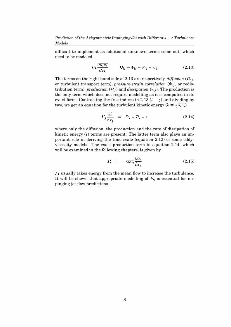
difficult to implement as additional unknown terms come out, whichneed to be modeled

� �� (2.13)

The terms on the right hand side of 2.13 are respectively, diffusion ( � �� ,or turbulent transport term), pressure-strain correlation ( � �� , or redis-tribution term), production (

� �� ) and dissipation ( � �� ). The production isthe only term which does not require modelling as it is computed in itsexact form. Contracting the free indices in 2.13 ( � �� ) and dividing bytwo, we get an equation for the turbulent kinetic energy ( � ��

�� )� � � �� (2.14)

where only the diffusion, the production and the rate of dissipation ofkinetic energy ( � ) terms are present. The latter term also plays an im-portant role in deriving the time scale (equation 2.12) of some eddy-viscosity models. The exact production term in equation 2.14, whichwill be examined in the following chapters, is given by

� � � � �� (2.15)

� �usually takes energy from the mean flow to increase the turbulence.

It will be shown that appropriate modelling of� �

is essential for im-pinging jet flow predictions.

8

Chapter 3

Turbulence ModelsConsidered

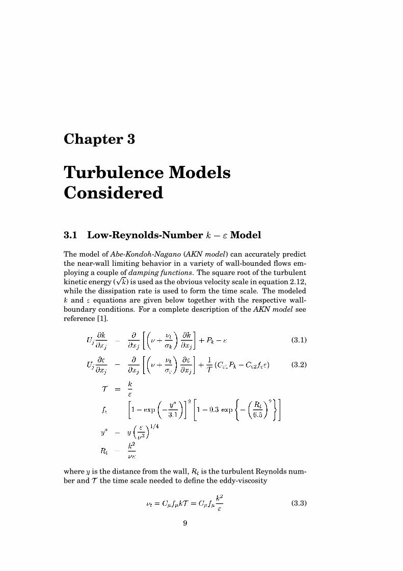
3.1 Low-Reynolds-Number � � � Model

The model of Abe-Kondoh-Nagano (AKN model) can accurately predictthe near-wall limiting behavior in a variety of wall-bounded flows em-ploying a couple of damping functions. The square root of the turbulentkinetic energy ( � � ) is used as the obvious velocity scale in equation 2.12,while the dissipation rate is used to form the time scale. The modeled� and � equations are given below together with the respective wall-boundary conditions. For a complete description of the AKN model seereference [1].

� � � �� , 5�� 5 �� 1 � �� (3.1)

� � � �� , 5�� 5�� 1 � ��

�� $ (3.2)

� � ��

� � �� , �� 1 � �� !� �� , � �� 1 ��

� � �� 5�� 5 �

where is the distance from the wall, � � is the turbulent Reynolds num-ber and � the time scale needed to define the eddy-viscosity

5 � � � � � � � � � � � � � � �� (3.3)

9


and �� the damping function to take into account the near-wall effectson 5�

� � �� , � �� 1 � ��

� � � �� , � �� 1 � � �The constants of the model are given in the following table:

� � � � � �� The production term (equation 2.15) is computed using the Boussi-

nesq assumption (2.11) as

� � � � 5� � � (3.4)

where � �� 2� � �� , is the mean strain-rate magnitude.

Wall Boundary Conditions

The turbulent kinetic energy goes to zero at the wall whereas � retainsa finite value on the wall surface according to the near wall limitingbehavior

�� (3.5)

�� 5 � � � � (3.6)

the indices � and � denote the wall and the nearest grid point from thewall, respectively. A complete derivation of the � boundary conditionis found in references [1] and [17].

3.2 Standard �� Model

The �� (or � �� ) model does not use the damping functions of theprevious section to solve the � and � equations (setting � � � � on theright hand side of equation 3.2, we get the standard � �� model). In-stead, a wall-normal Reynolds stress ( � ) is introduced together with anelliptic relaxation function ( � ) which handles the wall damping effectson the stress component. Then, an additional modeled transport equa-tion must be solved for the � stress, which is derived from the exactReynolds stress transport equation, especially looking at the redistri-bution term in equation 2.13 to take into account the damping effects.A detailed description of the �� model along with its derivation isfound in references [12] and [16].

10

CHAPTER 3. TURBULENCE MODELS CONSIDERED

� �� , 5�� 5�� 1 � �� (3.7)

� � � � ��

��

��

�

� � ��

�� (3.8)

The time ( � ) and length (�

) scales are given by

� � �� , � � " �� 5�1 (3.9)

� � �� "�� , 5 �� 1 �� (3.10)

where the time-scale has been bounded such that it will not be smallerthan the Kolmogorov time-scale ( �� 5 � � ). This limit guarantees toavoid singularities in the governing equations as the wall is approached.Making use of the new velocity scale ( � � � � $ �� ), the eddy-viscosity isdefined as 5� � � � �� (3.11)

The “constant” � � � (equation 3.2) is also damped near the wall accordingto

� � � � � �� , � � � �� 1 (3.12)

and the remaining constants of the model are listed on the table below:

� � � � ��

Wall Boundary Conditions

The � and � wall boundary conditions are the same as the ones givenby equations 3.5 and 3.6 in the AKN model. Besides, the wall-normalReynolds stress and the relaxation function go to zero at the wall for themodeled equations considered here [16]

� � � (3.13)

� � � (3.14)

11


3.3 Realizable � � � � Model

The modeled production of kinetic energy (equation 3.4) becomes verylarge at the stagnation region due to the high value of the strain-ratemagnitude, � . That is the reason why the turbulent kinetic energy ishigh at this point. On the other hand, it should be checked that allthe normal stresses remain positive, say �� . Durbin [13] imposeda time scale constraint for the � � � model based on this realizablecriteria which is of great importance for EVM in stagnation flow. TheBoussinesq assumption (equation 2.11) for the normal stress to the im-pingement wall (see Figure 1.1) can be simplified to ��

� �"� � 5 � � � � (3.15)

If � � � gets too large, then �� which is unphysical. Thus, let’s ex-amine when � � � becomes largest. The symmetric strain-rate tensor � ��has real eigenvalues and is diagonal in principal-axes coordinates. Thediagonal elements of � �� in the rotated coordinate system are its eigen-values ( �� "�� " � ) which can be found solving the equation

�� (3.16)

In two dimensions, the solution of 3.16 along with the incompressibleflow assumption ( � � � � � � � �� , equation 2.7) gives

� ��

�� (3.17)

As all the strains are now normal, equation 3.15 results in (also impos-ing the realizability constraint) ��

� �"� � 5 � � ��

5 � �� (3.18)

The equation above gives a bound on the eddy-viscosity. If the definitionof 5� for the � � � model is now used (equation 3.11) together withequation 3.17, the following constraint on the time scale � comes about

� ��

�� (3.19)

The derived constraint on � lowers its value, leading to a smaller eddy-viscosity which counteracts the high strain-rates. This is the way theproduction of kinetic energy is diminished in the stagnation region. Fi-nally, equations 3.9 and 3.19 can be merged to fulfil all the turbulent

12


time scale demands (a model constant is also added on equation 3.19,see reference [16])

� � �� , � � " �� 5�1 " � � � �� (3.20)

A similar realizable condition has been also proposed for the lengthscale

�[16], and it reads� � �� " � � � �� "

�� , 5 �� 1 �� (3.21)

Although it was implemented, it was found that the limitation on�

isnot as significant as that for

�.

Implementing the Realizability Constraint for the � � ��Model

Equation 3.8 is of elliptic character so that disturbances in one pointpropagate throughout the whole computational domain. Due to the in-tricate coupling between equations 3.7 and 3.8 along with the time scalelimit of 3.20, the computations are likely to diverge if the realizabilityconstraint is not implemented in a compatible manner. The main reasonwhy a given simulation might diverge is directly related to the magni-tude of � in the domain. If � gets too large, then the source term � �in equation 3.7 increases the production of the normal stress such that � � � � � which also have a feedback on � [17]. To overcome this issue, theright hand side of 3.8 (its source term) can be used as an upper boundon � for the term � � in the � equation [9]

�� " � �� $ �� $ � � � ��

�� (3.22)

where � is the old time scale (equation �� ) without the realizabilitycondition for stagnation flow. Instead of explicitly using the constrainton � in equations 3.7 and 3.8, it is imposed for the ratio � � � as

��

��

" � � �� " � � (3.23)

This limit is only used in the � and � equations together with the oldtime scale given in equation �� . For the � and � equations the new timescale limit is turned on (equation 3.20) as well as for the definition ofthe eddy-viscosity (equation 3.11).

13


3.4 Time Scale Constraint for Low-Reynolds-Number Model

It will be shown in chapter 5 that the computations carried out with therealizable �� model are in good agreement with the experimentaldata. Thus, it is suggested to modify the original time scale in the low-Reynolds number � � � model (AKN model) to dampen the productionof kinetic energy at the stagnation point. In section 3.1 was defined theeddy-viscosity for the AKN model. If that definition (equation 3.3) issubstituted in the derivation of the realizability constraint (equations3.17 and 3.18), the following time scale limit arises

� ��

�� (3.24)

Combining the old time scale ( � �� ) with the new limit and afteradding a model constant, the time scale for the AKN model in impingingflow is given by

� � �� " � � �� (3.25)

3.5 Limiter for�� in Low-Reynolds-Number

Model

The time scale constraints presented in the previous sections have a di-rect effect on the eddy-viscosity which is proportional to the product ofa velocity scale (squared) and a time scale. Thus, the realizable condi-tion for stagnation flow works well in lowering the production rate of� (equation 3.4) when the time scale decreases. Instead of restrictingthe time scale, it is proposed to apply a limiter directly on the produc-tion of kinetic energy itself. This can be carried out via a bound on

� �,

which is expected to operate in the stagnation region. The (constant)limiter makes the production rate of � (equation 3.1) proportional to thedissipation rate ( � ) and is stated as,

� � � �� "�� (3.26)

where the old time scale ( � � � ) is used for all the equations of the AKNmodel as well as in the first part of equation 3.26. Impinging jet flowsimulations were performed to tune the limiter

�.

14


3.6 Turbulent heat flux

The model for the temperature-velocity fluctuations is also based on theBoussinesq assumption �� 5 �

� � �

�� (3.27)

where� � � is the turbulent Prandtl number. Replacing equation 3.27

into 2.10, yields the modeled temperature equation

� � � �� , 5

� �� 5��

1 �� (3.28)

The laminar and turbulent Prandtl numbers are set to 0.72 and 0.89,respectively for all the simulations.

15


16

Chapter 4

Computational Approach

4.1 The Solver

CALC-BFC (Boundary Fitted Coordinates) by Davidson and Farhanieh[8] is a CFD code for computations of two or three-dimensional steady/-unsteady, laminar/turbulent recirculating flows. The discretization tech-nique is based on the Finite Volume Method (FVM) depicted in [18] andthe main characteristics of the code are the use of a non-orthogonal coor-dinate system, the pressure-correction SIMPLE (Semi-Implicit Methodfor Pressure-Linked Equations) algorithm and the co-located grid ar-rangement with Rhie and Chow interpolation. A segregated Tri- Di-agonal Matrix Solver (TDMA) is employed to solved the discretized al-gebraic equations. Hybrid central/upwind differencing, the QUICK andthe Van Leer schemes are available for the discretization of the convec-tive terms. However, it was found out the Hybrid scheme to performgood enough for the simulations accomplished in this study.

4.2 Axisymmetry considerations

The general transport equation for a variable � ( � � � " � " � " � " � � ) insteady state can be written as�� $ �

�� ,�� 1 � � � (4.1)

where �� denotes the source per unit volume of the variable � and �is the diffusion coefficient. After performing the discretization of eachtransport equation, the corresponding algebraic equations have the fol-lowing form

�� (4.2)

where the index �� denotes the neighboring nodes of node�

and �� isthe source term. The coefficient at the node under consideration can be

17


��

+

+

�

��

�

��

��

��

�

� �

��

Figure 4.1: Modified control volume.

expressed (in two-dimensions) as

�� $ � � �

� � ��

where�

, � , � and � denote east, west, north and south respectively.Each coefficient contains the contribution due to convection and diffu-sion, and the general source term S which is split in a positive part ( �� )and negative part ( �

�) holds the terms.

Regardless of the scheme used to discretize the convective terms, thearea of each face of the control volume has to be corrected for the ax-isymmetric geometry of the impinging jet. For instance, the area of theeast face � � varies with the radial distance � and the area of the northface has to be computed according to cylindrical coordinates. Thesechanges are better understood if a single finite volume is consideredas in Figure 4.1. There is a clear correspondence between the cartesiancoordinates (

#" "�� ) and the cylindrical ones ( �" " � ) which comes after

correcting the areas of the east and north faces as follows [2]

� � � � � �� $ � � � �� $ � � � � � � $ ! �� $ � � � � � � ��$ � � � � � � $ ! �

��

�� $ � �

18

CHAPTER 4. COMPUTATIONAL APPROACH

where ��

is the radial (

-direction) location of the control volume andthe index �

��is used to designate the cartesian areas. Also, the volume

needs to be corrected as 0 � � � 0 � $ ! � � �The above changes ensure the right coefficients to be used in any of thealgebraic equations given by 4.2.

4.3 Numerical Method

Diffusion terms were approximated using central differencing and hy-brid central/upwind differencing or Van Leer was used for the discretiza-tion of convection in the momentum, temperature and turbulence equa-tions. However, no appreciable difference in the calculated fields was ob-served when Van Leer scheme was used. Thus, hybrid central/upwinddifferencing was kept as the suitable scheme for convection. The dy-namic and thermal fields are uncoupled in the impinging jet flow andtherefore the thermal field was solved only once the dynamic field hadconverged. Under-relaxation factors ( � � � � � ) were also used implic-itly

��

� ��

� ��

�� $ � � ��

Changes between successive iterations are slowed down using a suitable� in each discretized transport equation which stabilizes and improvesthe iterative process. Typical under-relaxation factors for the calcula-tions carried out in this study are shown in Tables 4.1 and 4.2.

� � � � � � 5��

Table 4.1: Under-relaxation factors used with the low-Reynolds numbermodel

� � � � � � � � 5��

Table 4.2: Under-relaxation factors used with the � � � model

19


� � � � � �

Impingement Wall

North Boundary

Outlet

Inlet

Sym

met

ryAx

is

�

�

��

� ��

Figure 4.2: Flow domain.

It was also required to increase the number of sweeps to be per-formed by the TDMA solver for the pressure ( � ) and radial velocity ( � )equations, to 30 and 5 sweeps respectively. This was executed in bothmodels and faster convergence was observed. Convergence was reachedwhen the total non-dimensionalized residuals for the momentum equa-tions were below �� . It was confirmed that reducing residuals belowthis value had no effect on results. Each residual is normalized by thetotal incoming flux of the dependent variable.

4.4 Domain and Boundary Conditions

Figure 4.2 is a sketch of the computational domain which shows a jetdischarge height of 2 jet diameters and a domain extension of 8 jet di-ameters in the radial direction.

A fine, non-uniform structured grid of ��! "� nodes was used witha high resolution near the impingement wall and in the vicinity of thesymmetry line where the jet evolves. A close-up of this region is shownin Figure 4.3. The clustered grid spacing at both size of #%$'& ()�"*+�is required to fit the inlet boundary conditions coming from a fully--developed pipe flow. Different grid configurations were tested to ensuregrid-independence, and the present grid was selected as the one whichprovides satisfactory results at a reasonable computational cost.

Figure 4.2 also outlines the boundary conditions employed in theimpinging jet flow.

20


X/D

Y/D

0 0.25 0.5 0.75 10

0.1

0.2

0.3

0.4

0.5

0.6

0.7

0.8

0.9

1

Figure 4.3: Focused view of the grid at the stagnation region.

Inlet Boundary

Fully-developed turbulent pipe flow with turbulent Reynolds number,�� (based on the friction velocity and jet diameter) was com-puted separately to obtain the velocity and turbulent kinetic energy pro-files as the inlet boundary conditions for each modeled assessed (Figure4.4). �� is chosen according to the pipe friction factor, so its value cor-responds to the experimental Reynolds number of 23000 (based on thebulk velocity and jet diameter) for the jet simulations. In this computa-tion, the grid spacing was chosen such that it perfectly fit the grid nodesat the inlet boundary of the impinging jet. The calculated profiles werenormalized by the bulk velocity computed as

� � � ��

� (4.3)

where � denotes the pipes cross sectional area.When calculating the thermal field, the inlet temperature was fixed

to a constant value (� � � � � ). Also, the radial velocity was set to zero

(� � � ) and Neumann condition was prescribed for the remaining vari-

ables as

, � �� 1 � � � � � � (4.4)

where is the axial direction (Figure 4.2) and � represents any of thevariables different from the axial velocity ( � ) and turbulent kinetic en-ergy ( � ) profiles already specified.

21


0 0.1 0.2 0.3 0.4 0.5

−1.2

−1

−0.8

−0.6

−0.4

−0.2

0

PSfrag replacements

��

��

V2F modelAKN model

0 0.1 0.2 0.3 0.4 0.50

0.005

0.01

0.015

PSfrag replacements

��

��

V2F modelAKN model

Figure 4.4: Inlet profiles.

Symmetry Axis

Along the axis of symmetry, zero-gradient (Neumann) condition was ap-plied for the axial velocity component, turbulent scalars and tempera-ture , � �� 1 �� (4.5)

To implement Neumann condition, the nodal value on the boundary ofthe domain was set equal to the neighboring nodal value inside the do-main. The radial velocity was set to zero at this boundary

� � � , sothere is no momentum flux across the symmetry line.

North Boundary

Slip condition was applied along this boundary. To implement this con-dition, the axial velocity was set to zero � � � . Neumman condition wasimplemented for the radial velocity component (

�), turbulent scalars

and temperature

, � �� 1 � � �� (4.6)

Outlet

At the right hand outlet boundary, zero gradient conditions were appliedto all the variables

, � �� 1 � � � � � � (4.7)

22


Although the flow through this boundary should be leaving the domain,during the iteration process flow is allowed to enter or exit through theboundary. Then, the velocity along this boundary is corrected in orderto satisfy global continuity.

Impingement Wall

The wall boundary conditions for the turbulence quantities were al-ready discussed in Chapter 3 for each model considered in this study.However, nothing was said concerning their implementation.

The boundary condition for the dissipation rate ( � ) is implementedimplicitly via its source term � (equation 4.2), while the value at thewall ( � � ) for the remaining turbulence quantities was explicitly as-signed to the nodes lying on this boundary.

Constant heat flux was applied along the wall and it was imple-mented via the source term � for the discretized temperature equa-tion. Besides, the south coefficient

� �is set to zero, so that no other

means of heat flux takes place.

23


24

Chapter 5

Results and Discussion

5.1 Performance of the Time Scale Constraint

0 0.5 10

0.1

0.2

0.3

0.4

0.5

r/D=0

PSfrag replacements

� ��

Standard AKNV2FRealizable AKNExperiments

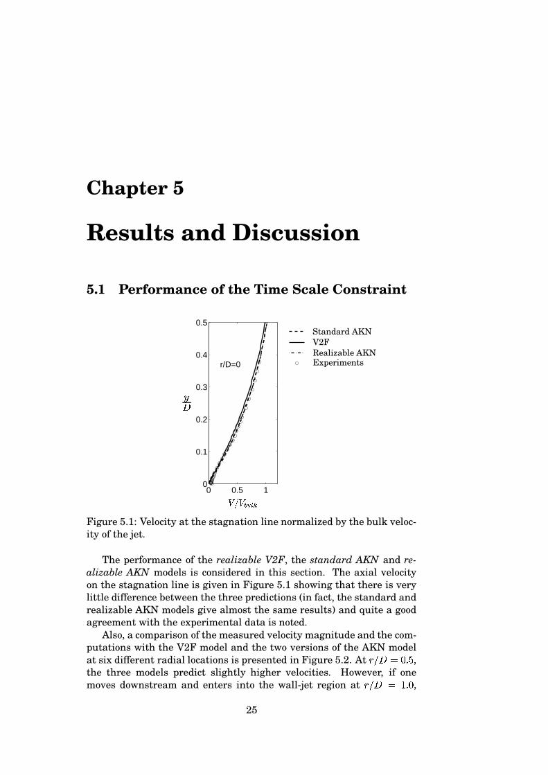
Figure 5.1: Velocity at the stagnation line normalized by the bulk veloc-ity of the jet.

The performance of the realizable V2F, the standard AKN and re-alizable AKN models is considered in this section. The axial velocityon the stagnation line is given in Figure 5.1 showing that there is verylittle difference between the three predictions (in fact, the standard andrealizable AKN models give almost the same results) and quite a goodagreement with the experimental data is noted.

Also, a comparison of the measured velocity magnitude and the com-putations with the V2F model and the two versions of the AKN modelat six different radial locations is presented in Figure 5.2. At � �� ,the three models predict slightly higher velocities. However, if onemoves downstream and enters into the wall-jet region at � �� ,

25


0 0.5 10

0.05

0.1

0.15

0.2

0.25

0.3

0.35

0.4

0.45

0.5

r/D=0.5

PSfrag replacements

� ��

��

0 0.5 10

0.05

0.1

0.15

0.2

0.25

0.3

0.35

0.4

0.45

0.5

r/D=1.0

PSfrag replacements

� ��

��

0 0.5 10

0.05

0.1

0.15

0.2

0.25

0.3

0.35

0.4

0.45

0.5

r/D=1.5

PSfrag replacements

� ��

��

0 0.5 10

0.05

0.1

0.15

0.2

0.25

0.3

0.35

0.4

0.45

0.5

r/D=2.0

PSfrag replacements

� ��

��

0 0.5 10

0.05

0.1

0.15

0.2

0.25

0.3

0.35

0.4

0.45

0.5

r/D=2.5

PSfrag replacements

� ��

��

0 0.5 10

0.05

0.1

0.15

0.2

0.25

0.3

0.35

0.4

0.45

0.5

r/D=3.0

PSfrag replacements

� ��

��

Figure 5.2: Profiles of the normalized velocity magnitude at differentradial locations. Key as Figure 5.1.

the velocity magnitude increases from a value of zero to some maxi-mum and subsequently decays to a very small value. The V2F and therealizable AKN models correctly predict the flow acceleration; there isexcellent agreement with the data at this location. The standard AKNmodel predicts slightly lower velocities in the wall region and highervelocities in the outer region. Farther downstream, it can be noticeda better match between the V2F and the realizable AKN models withthe experimental data. The standard AKN model carries on predictinglower velocities near the wall and higher velocities in the outer region,all the way downstream. As can be seen, the realizable AKN model per-forms much better than the standard AKN model when considering thevelocity profiles.

26

CHAPTER 5. RESULTS AND DISCUSSION

0 0.02 0.040

0.05

0.1

0.15

0.2

0.25

0.3

0.35

0.4

r/D=0.5

PSfrag replacements

��

��

0 0.02 0.040

0.05

0.1

0.15

0.2

0.25

0.3

0.35

0.4

r/D=1.0

PSfrag replacements

��

��

0 0.02 0.040

0.05

0.1

0.15

0.2

0.25

0.3

0.35

0.4

r/D=1.5

PSfrag replacements

��

��

0 0.02 0.040

0.05

0.1

0.15

0.2

0.25

0.3

0.35

0.4

r/D=2.0

PSfrag replacements

��

��

0 0.02 0.040

0.05

0.1

0.15

0.2

0.25

0.3

0.35

0.4

r/D=2.5

PSfrag replacements

��

��

0 0.02 0.040

0.05

0.1

0.15

0.2

0.25

0.3

0.35

0.4

r/D=3.0

PSfrag replacements

��

��

Figure 5.3: Normalized wall-parallel Reynolds stress profiles at differ-ent radial locations. Key as Figure 5.1.

The development of the Reynolds stresses as the flow develops awayfrom the stagnation point is presented in Figures 5.3 to 5.5. Lookingat the wall-parallel Reynolds stress profiles of Figure 5.3, it can be saidthat none of the models perfectly matches the experimental data. Nev-ertheless, the predicted profiles at � �� and � �� given by theV2F and realizable AKN models are reasonably good, especially in thewall region. On the other hand, the standard AKN model predicts toohigh � values at these two particular locations. The V2F gives quitegood results even though the Boussinesq assumption (equation 2.11) isemployed to compute this stress and again, very little difference is ob-served between the profiles given by the V2F and the realizable AKNmodels.

27


0 0.02 0.04 0.06 0.080

0.05

0.1

0.15

0.2

0.25

0.3

0.35

0.4

r/D=0.5

PSfrag replacements

� ��

��

0 0.02 0.040

0.05

0.1

0.15

0.2

0.25

0.3

0.35

0.4

r/D=1.0

PSfrag replacements

� ��

��

0 0.02 0.040

0.05

0.1

0.15

0.2

0.25

0.3

0.35

0.4

r/D=2.5

PSfrag replacements

� ��

��

0 0.02 0.040

0.05

0.1

0.15

0.2

0.25

0.3

0.35

0.4

r/D=3.0

PSfrag replacements

� ��

��

Figure 5.4: Normalized wall-normal Reynolds stress profiles at differentradial locations. Key as Figure 5.1.

The differences between the models are more appreciable when look-ing at the wall-normal stress profiles of Figure 5.4. It is evident that theperformance of the V2F model is outstanding compared to both versionsof the AKN model. The main reason is due to the implementation of a � transport equation in the V2F model instead of using the Boussinesqassumption. However, it should be noticed the improved prediction ob-tained by the realizable AKN not too far from the stagnation line (at� �� and � �� ). It can be noticed that the V2F model yieldsa moderate anisotropy between the wall-parallel stress component seenin Figure 5.3 and the wall-normal component, especially for the firsttwo profiles. Once again, the results given by the standard AKN modelconsiderably deviate from the measured data.

28


−0.02 0 0.020

0.05

0.1

0.15

0.2

0.25

0.3

0.35

0.4

r/D=0.5

PSfrag replacements

� � ��

��

−0.02 0 0.020

0.05

0.1

0.15

0.2

0.25

0.3

0.35

0.4

r/D=1.0

PSfrag replacements

� � ��

��

−0.02 0 0.020

0.05

0.1

0.15

0.2

0.25

0.3

0.35

0.4

r/D=2.5

PSfrag replacements

� � ��

��

−0.02 0 0.020

0.05

0.1

0.15

0.2

0.25

0.3

0.35

0.4

r/D=3.0

PSfrag replacements

� � ��

��

Figure 5.5: Normalized turbulent shear stress profiles at different ra-dial locations. Key as Figure 5.1.

A similar behavior can be observed from the turbulent shear stressprofiles of Figure 5.5. Again, the V2F and realizable AKN models givethe most accurate account of the development, with the standard AKNmodel being less successful in matching the experimental data, thoughnot as spectacularly so as for � .

Measurements of the wall-normal Reynolds stress at the symmetry(stagnation) line are compared in Figure 5.6 with � � � � from the twoversions of the AKN model and the V2F model calculations, as well as�� from V2F computations. This figure clearly shows that � predictionsin the vicinity of the stagnation point obtained from the standard AKNmodel are one order of magnitude higher than � , hence this model ex-ceedingly over-estimates the fluctuating quantities and heat transfer

29


0 0.01 0.02 0.03 0.04 0.050

0.05

0.1

0.15

0.2

0.25

0.3

0.35

0.4

0.45

0.5

PSfrag replacements

��

� � , with V2F� �� , with V2F� �� , Realizable AKN� �� , Standard AKN� � , Experiments

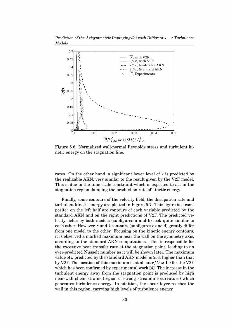
Figure 5.6: Normalized wall-normal Reynolds stress and turbulent ki-netic energy on the stagnation line.

rates. On the other hand, a significant lower level of � is predicted bythe realizable AKN, very similar to the result given by the V2F model.This is due to the time scale constraint which is expected to act in thestagnation region damping the production rate of kinetic energy.

Finally, some contours of the velocity field, the dissipation rate andturbulent kinetic energy are plotted in Figure 5.7. This figure is a com-posite: on the left half are contours of each variable predicted by thestandard AKN and on the right predictions of V2F. The predicted ve-locity fields by both models (subfigures a and b) look quite similar toeach other. However, � and � contours (subfigures c and d) greatly differfrom one model to the other. Focusing on the kinetic energy contours,it is observed a marked maximum near the wall on the symmetry axis,according to the standard AKN computations. This is responsible forthe excessive heat transfer rate at the stagnation point, leading to anover-predicted Nusselt number as it will be shown later. The maximumvalue of � predicted by the standard AKN model is 55% higher than thatby V2F. The location of this maximum is at about � �� for the V2Fwhich has been confirmed by experimental work [4]. The increase in theturbulent energy away from the stagnation point is produced by highnear-wall shear strains (region of strong streamline curvature) whichgenerates turbulence energy. In addition, the shear layer reaches thewall in this region, carrying high levels of turbulence energy.

30


−2 −1 0 1 20

0.5

1

1.5

2

PSfrag replacements

��

��

Standard AKN V2F

(a) Axial Velocity, ��

−8 −6 −4 −2 0 2 4 6 80

0.5

1

1.5

2

PSfrag replacements

��

��

Standard AKN V2F

(b) Radial Velocity, ��

−4 −2 0 2 40

0.5

1

1.5

2

PSfrag replacements

��

��

Standard AKN V2F

(c) Dissipation rate, ��

−4 −2 0 2 40

0.5

1

1.5

2

0.0450.07

PSfrag replacements

� ��

��

Standard AKN V2F

(d) Turbulent Kinetic Energy, ��

Figure 5.7: Comparison of various contours obtained from two differentturbulence models.

5.2 Limiter effect on the AKN model

Here is described how the limiter�

in equation 3.26 was optimized. Sev-eral simulations were carried out for different values of

�, ranging from

1.5 to 15 and the results were compared with the existing calculationsobtained from the standard and realizable AKN models. The resultspresented below correspond to the most distinctive limiters found inthis study, that is to say

� � �� " � and �� .The axial velocity on the symmetry line shown in Figure 5.8 indi-

cates no limiter dependence as there is no perceptible difference be-tween the three predictions, as well as very good agreement with themeasured data is noticed. However, the predicted velocity profiles down-

31


0 0.5 10

0.1

0.2

0.3

0.4

0.5

r/D=0

PSfrag replacements

� � ��

��

Experiments

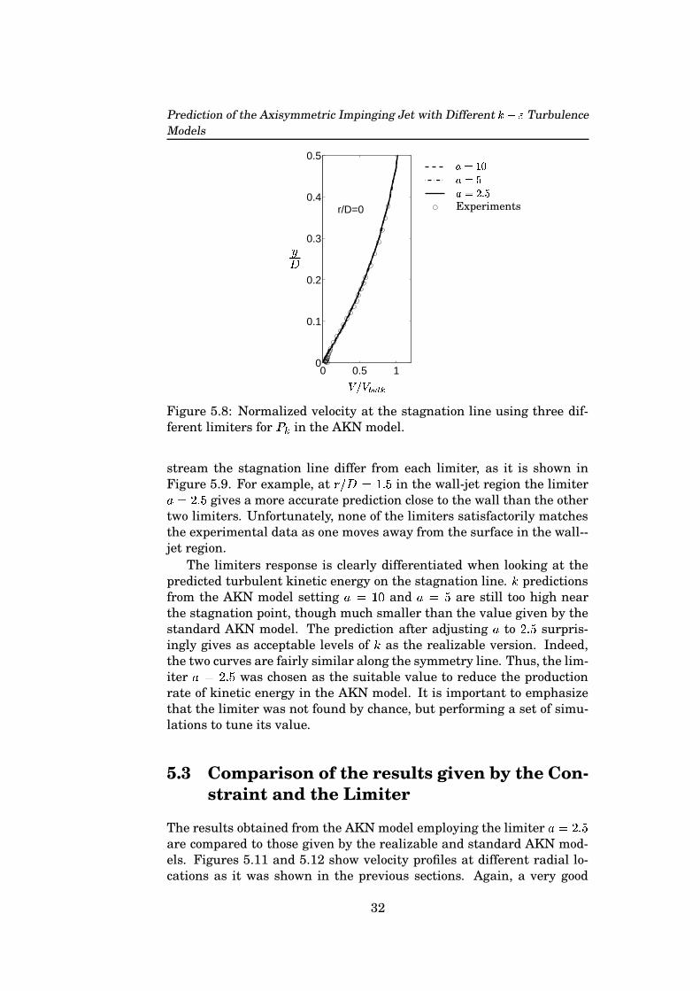
Figure 5.8: Normalized velocity at the stagnation line using three dif-ferent limiters for

� �in the AKN model.

stream the stagnation line differ from each limiter, as it is shown inFigure 5.9. For example, at � �� in the wall-jet region the limiter� � �� gives a more accurate prediction close to the wall than the othertwo limiters. Unfortunately, none of the limiters satisfactorily matchesthe experimental data as one moves away from the surface in the wall--jet region.

The limiters response is clearly differentiated when looking at thepredicted turbulent kinetic energy on the stagnation line. � predictionsfrom the AKN model setting

� � �� and� � � are still too high near

the stagnation point, though much smaller than the value given by thestandard AKN model. The prediction after adjusting

�to �� surpris-

ingly gives as acceptable levels of � as the realizable version. Indeed,the two curves are fairly similar along the symmetry line. Thus, the lim-iter

� � �� was chosen as the suitable value to reduce the productionrate of kinetic energy in the AKN model. It is important to emphasizethat the limiter was not found by chance, but performing a set of simu-lations to tune its value.

5.3 Comparison of the results given by the Con-straint and the Limiter

The results obtained from the AKN model employing the limiter� � ��

are compared to those given by the realizable and standard AKN mod-els. Figures 5.11 and 5.12 show velocity profiles at different radial lo-cations as it was shown in the previous sections. Again, a very good

32


0 0.5 10

0.05

0.1

0.15

0.2

0.25

0.3

0.35

0.4

0.45

0.5

r/D=0.5

PSfrag replacements

� � ��

��

0 0.5 10

0.05

0.1

0.15

0.2

0.25

0.3

0.35

0.4

0.45

0.5

r/D=1.0

PSfrag replacements

� � ��

��

0 0.5 10

0.05

0.1

0.15

0.2

0.25

0.3

0.35

0.4

0.45

0.5

r/D=1.5

PSfrag replacements

� � � ��

��

0 0.5 10

0.05

0.1

0.15

0.2

0.25

0.3

0.35

0.4

0.45

0.5

r/D=2.0

PSfrag replacements

� � ��

��

0 0.5 10

0.05

0.1

0.15

0.2

0.25

0.3

0.35

0.4

0.45

0.5

r/D=2.5

PSfrag replacements

� � ��

��

0 0.5 10

0.05

0.1

0.15

0.2

0.25

0.3

0.35

0.4

0.45

0.5

r/D=3.0

PSfrag replacements

� � � ��

��

Figure 5.9: Limiter effect on velocity profiles, AKN model. Key as Fig-ure 5.8.

agreement with the measured data is observed on the stagnation linefor all the AKN versions. Downstream is noted the remarkable perfor-mance of the realizable version in predicting the velocity profiles, eventhough the limiter also improves the predictions compared to the resultsgiven by the standard AKN version. The development of the Reynoldsstresses as the flow develops away from the stagnation point is pre-sented in Figures 5.13 to 5.15. When looking at the three different setsof stress profiles, it can be noticed the predicted results given by thelimiter are in between those given by the realizable and standard mod-els. As it was expected, the realizable and limiter AKN models providemuch better results in the stagnation region than those of the standardAKN model. Besides, far from the stagnation point (at � �� ) theresults given by the three AKN versions differ very little, which means

33


0 0.005 0.01 0.015 0.02 0.025 0.030

0.05

0.1

0.15

0.2

0.25

0.3

0.35

0.4

0.45

0.5

PSfrag replacements

��

� �� , Realizable

� � , Experiments

Figure 5.10: Limiter effect on the stagnation line, AKN model.

0 0.5 10

0.1

0.2

0.3

0.4

0.5

r/D=0

PSfrag replacements

� � � ��

StandardLimiter, ��

RealizableExperiments

Figure 5.11: Normalized velocity at the stagnation line predicted bythree versions of the AKN model.

a weak influence from the upstream conditions.In addition, a comparison of the turbulent kinetic energy contours is

shown in Figure 5.16. It is well noted the resemblance of the contoursgiven by the realizable condition and the limiter. Also, the maximumoccurs away from the stagnation line; both predicted values differ only

34


0 0.5 10

0.05

0.1

0.15

0.2

0.25

0.3

0.35

0.4

0.45

0.5

r/D=0.5

PSfrag replacements

� � ��

��

0 0.5 10

0.05

0.1

0.15

0.2

0.25

0.3

0.35

0.4

0.45

0.5

r/D=1.0

PSfrag replacements

� � ��

��

0 0.5 10

0.05

0.1

0.15

0.2

0.25

0.3

0.35

0.4

0.45

0.5

r/D=1.5

PSfrag replacements

� � � ��

��

0 0.5 10

0.05

0.1

0.15

0.2

0.25

0.3

0.35

0.4

0.45

0.5

r/D=2.0

PSfrag replacements

� � ��

��

0 0.5 10

0.05

0.1

0.15

0.2

0.25

0.3

0.35

0.4

0.45

0.5

r/D=2.5

PSfrag replacements

� � ��

��

0 0.5 10

0.05

0.1

0.15

0.2

0.25

0.3

0.35

0.4

0.45

0.5

r/D=3.0

PSfrag replacements

� � � ��

��

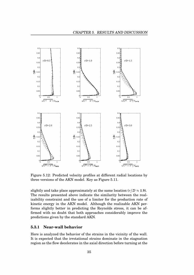
Figure 5.12: Predicted velocity profiles at different radial locations bythree versions of the AKN model. Key as Figure 5.11.

slightly and take place approximately at the same location ( � �� ).The results presented above indicate the similarity between the real-izability constraint and the use of a limiter for the production rate ofkinetic energy in the AKN model. Although the realizable AKN per-forms slightly better in predicting the Reynolds stress, it can be af-firmed with no doubt that both approaches considerably improve thepredictions given by the standard AKN.

5.3.1 Near-wall behavior

Here is analyzed the behavior of the strains in the vicinity of the wall.It is expected that the irrotational strains dominate in the stagnationregion as the flow decelerates in the axial direction before turning at the

35


0 0.02 0.040

0.05

0.1

0.15

0.2

0.25

0.3

0.35

0.4

r/D=0.5

PSfrag replacements

��

��

0 0.02 0.040

0.05

0.1

0.15

0.2

0.25

0.3

0.35

0.4

r/D=1.0

PSfrag replacements

��

��

0 0.02 0.040

0.05

0.1

0.15

0.2

0.25

0.3

0.35

0.4

r/D=1.5

PSfrag replacements

��

��

0 0.02 0.040

0.05

0.1

0.15

0.2

0.25

0.3

0.35

0.4

r/D=2.0

PSfrag replacements

��

��

0 0.02 0.040

0.05

0.1

0.15

0.2

0.25

0.3

0.35

0.4

r/D=2.5

PSfrag replacements

��

��

0 0.02 0.040

0.05

0.1

0.15

0.2

0.25

0.3

0.35

0.4

r/D=3.0

PSfrag replacements

��

��

Figure 5.13: Predicted wall-parallel Reynolds stress profiles at differentradial locations by three versions of the AKN model. Key as Figure 5.11.

wall. So, the normal strain� � � � represents an important contribution

when calculating the wall-normal stress

� � �� !� 5 � � �� (5.1)

This is verified looking at the results given by the three versions of theAKN model in the stagnation region seen in Figure 5.17. � � � � is alsoplotted for comparison. The normal strain has a negative value due tothe flow deceleration in the proximity of the wall, which increases thewall-normal stress of equation 5.1. The three AKN versions point outthe same trend to a more or less extent.

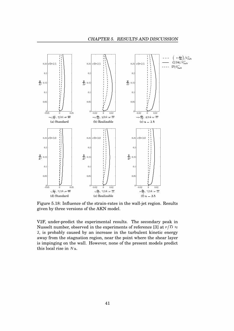
The opposite behavior is observed when looking at the results in thewall-jet region of Figure 5.18. Far from the stagnation point, the flow

36


0 0.02 0.04 0.06 0.080

0.05

0.1

0.15

0.2

0.25

0.3

0.35

0.4

r/D=0.5

PSfrag replacements

� ��

��

0 0.02 0.040

0.05

0.1

0.15

0.2

0.25

0.3

0.35

0.4

r/D=1.0

PSfrag replacements

� ��

��

0 0.02 0.040

0.05

0.1

0.15

0.2

0.25

0.3

0.35

0.4

r/D=2.5

PSfrag replacements

� ��

��

0 0.02 0.040

0.05

0.1

0.15

0.2

0.25

0.3

0.35

0.4

r/D=3.0

PSfrag replacements

� ��

��

Figure 5.14: Predicted wall-normal Reynolds stress profiles at differentradial locations by three versions of the AKN model. Key as Figure 5.11.

develops as a boundary layer flow dominated by the shear strains � � 5 � , � �� 1 (5.2)

Now the strain� � � � becomes important. As can be also seen, the nor-

mal strain� � � � goes to zero in the wall-jet region. This trend is accu-

rately predicted by all versions of the AKN model. Thus, shear replacesnormal straining as the principal energy generation mechanism.

5.3.2 Time-Scale Constraint and Limiter operation

The use of the different time-scales and the limiter (� � �� ) in the do-

main are shown in Figure 5.19 for both AKN versions. For comparison,

37


−0.02 0 0.020

0.05

0.1

0.15

0.2

0.25

0.3

0.35

0.4

r/D=0.5

PSfrag replacements

� � ��

��

−0.02 0 0.020

0.05

0.1

0.15

0.2

0.25

0.3

0.35

0.4

r/D=1.0

PSfrag replacements

� � ��

��

−0.02 0 0.020

0.05

0.1

0.15

0.2

0.25

0.3

0.35

0.4

r/D=2.5

PSfrag replacements

� � ��

��

−0.02 0 0.020

0.05

0.1

0.15

0.2

0.25

0.3

0.35

0.4

r/D=3.0

PSfrag replacements

� � ��

��

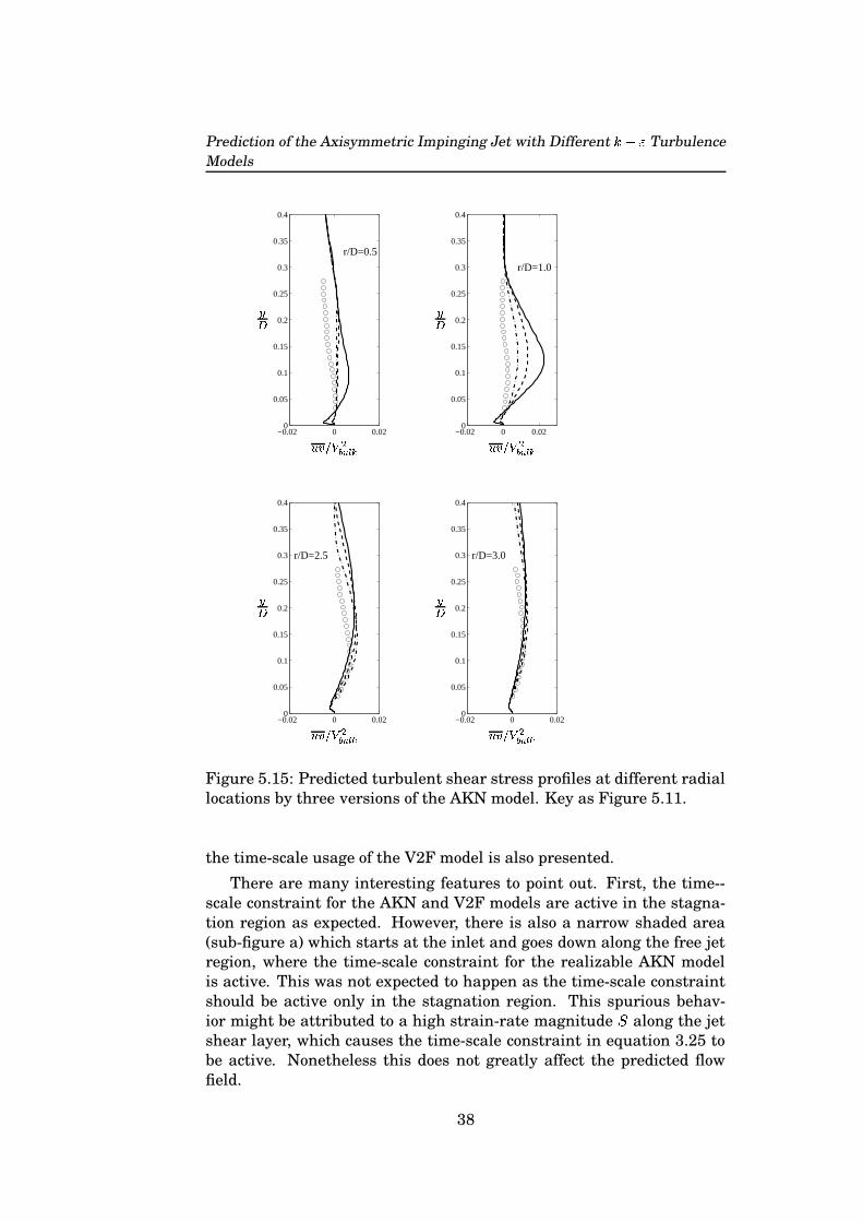
Figure 5.15: Predicted turbulent shear stress profiles at different radiallocations by three versions of the AKN model. Key as Figure 5.11.

the time-scale usage of the V2F model is also presented.

There are many interesting features to point out. First, the time--scale constraint for the AKN and V2F models are active in the stagna-tion region as expected. However, there is also a narrow shaded area(sub-figure a) which starts at the inlet and goes down along the free jetregion, where the time-scale constraint for the realizable AKN modelis active. This was not expected to happen as the time-scale constraintshould be active only in the stagnation region. This spurious behav-ior might be attributed to a high strain-rate magnitude � along the jetshear layer, which causes the time-scale constraint in equation 3.25 tobe active. Nonetheless this does not greatly affect the predicted flowfield.

38


−4 −2 0 2 40

0.5

1

1.5

2

0.0450.07PSfrag replacements

� � �

��

Standard Realizable

Limiter

−4 −2 0 2 40

0.5

1

1.5

2

0.050.045PSfrag replacements

� ��

��

Standard

Realizable Limiter ��

Figure 5.16: Comparison of turbulent kinetic energy contours obtainedfrom three versions of the AKN model.

On the other hand, the limiter� � �� only works at the stagnation

region as it is depicted in sub-figure b. In fact, the shaded area wherethe limiter is used in the domain resembles a lot to that where the V2Ftime-scale constraint acts to lower the production rate of � (sub-figurec).

Also, the V2F highlights the use of the Kolmogorov limiter in equa-tion 3.20 which is used in the near-wall region as well as close to the jetinlet, along a short and narrow area which is due to the convected pipeflow.

5.4 Heat transfer coefficient

If� �� , convection heat transfer occurs in both the stagnation

and wall-jet region. The Nusselt number in the impinging jet flow isevaluated as

� � � ��

� � �� $ � � �( � � �� $ (5.3)

where the ratio of the constant heat flux � �� to the specific heat � �is prescribed to calculate the Nusselt number, as the discretized equa-tion of temperature is already normalized by � � in the code. The walltemperature is estimated as� ��

� � � � � �� $ � �( (5.4)

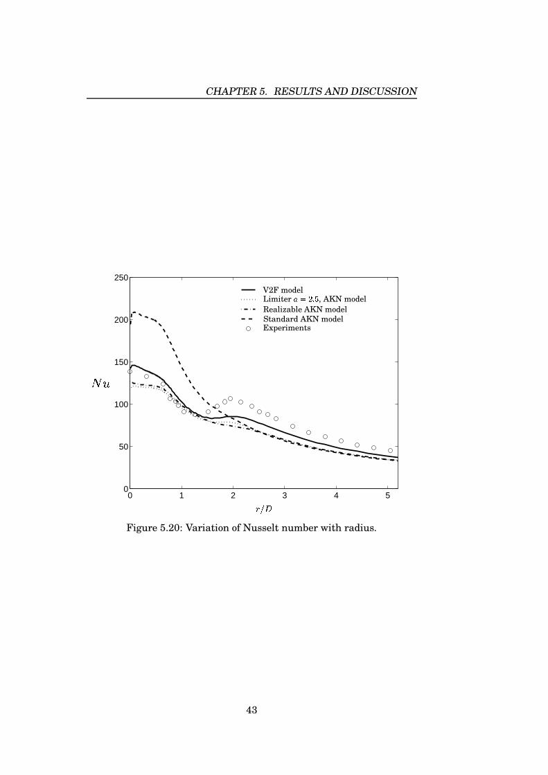
where the index 1 denotes the nearest grid point from wall surface.The predicted Nusselt number along the wall by the different tur-

bulence models is shown in Figure 5.20. None of the models perfectlymatches the experimental data, however big differences are observed

39


−0.05 0 0.050

0.05

0.1

0.15

0.2

0.25 r/D=0.25

PSfrag replacements

� ��

��

(a) Standard

−0.01 0 0.010

0.05

0.1

0.15

0.2

0.25 r/D=0.25

PSfrag replacements

� ��

��

(b) Realizable

−0.01 0 0.010

0.05

0.1

0.15

0.2

0.25 r/D=0.25

PSfrag replacements

� ��

��

�� ! �"#%$'&)(* +�, -. / $'021435$'&�(* +�, -687 $'&)(* +�, -

(c) �:9 �<; =

−0.05 0 0.050

0.05

0.1

0.15

0.2

0.25 r/D=0.5

PSfrag replacements

� ��

��

(d) Standard

−0.02 0 0.020

0.05

0.1

0.15

0.2

0.25 r/D=0.5

PSfrag replacements

� ��

��

(e) Realizable

−0.02 0 0.020

0.05

0.1

0.15

0.2

0.25 r/D=0.5

PSfrag replacements

� ��

��

(f) �>9 �<; =Figure 5.17: Influence of the strain-rates in the stagnation region. Re-sults given by three versions of the AKN model.

to one another. The heat transfer rate is greatest at the stagnationpoint, with � at its maximum. Nevertheless, � is significantly over-predicted by the standard AKN model. In this model, the stagnationNusselt number is about � �@? higher than the measured value, whereasthe V2F model prediction is only �%? too high. This high predicted valuegiven by the standard AKN model is due to the spurious kinetic energymaximum at the stagnation point illustrated in Figures 5.6 and 5.7.

On the other hand, the realizable AKN and the limiter under-predictthe Nusselt number at the stagnation point by

� ��)? and � �%? respec-tively. Again, it should be noted the resemblance in the predicted Nus-selt number given by these two AKN versions.

Downstream of the stagnation region the standard AKN Nusseltnumber rapidly decreases and approaches the predicted values of theother two AKN versions. For � �� all the models, including the

40


−0.05 0 0.050

0.05

0.1

0.15

0.2

0.25 r/D=2.5

PSfrag replacements

� ��

��

(a) Standard

−0.02 0 0.020

0.05

0.1

0.15

0.2

0.25 r/D=2.5

PSfrag replacements

� ��

��

(b) Realizable

−0.02 0 0.020

0.05

0.1

0.15

0.2

0.25 r/D=2.5

PSfrag replacements

� ��

��

� � �� ! �"<# $'& (* +�, -. / $�0<143�$'& (* +�, -6 7 $�& (* +�, -

(c) �:9 �<; =

−0.05 0 0.050

0.05

0.1

0.15

0.2

0.25 r/D=3.0

PSfrag replacements

� ��

��

(d) Standard

−0.02 0 0.020

0.05

0.1

0.15

0.2

0.25 r/D=3.0

PSfrag replacements

� ��

��

(e) Realizable

−0.02 0 0.020

0.05

0.1

0.15

0.2

0.25 r/D=3.0

PSfrag replacements

� ��

��

(f) �:9 �<; =Figure 5.18: Influence of the strain-rates in the wall-jet region. Resultsgiven by three versions of the AKN model.

V2F, under-predict the experimental results. The secondary peak inNusselt number, observed in the experiments of reference [3] at � �� , is probably caused by an increase in the turbulent kinetic energyaway from the stagnation region, near the point where the shear layeris impinging on the wall. However, none of the present models predictthis local rise in � .

41


0 2 4 6 80

0.5

1

1.5

2

PSfrag replacements

� ��

��

(a) Realizable AKN model

0 2 4 6 80

0.5

1

1.5

2

PSfrag replacements

� ��

��

� � ��

(b) Limiter �� , AKN model

0 2 4 6 80

0.5

1

1.5

2

PSfrag replacements

� ��

��

� � ! "

� � � � ! "

(c) V2F model

Figure 5.19: Regions where constraints are active (colored white).

42


0 1 2 3 4 50

50

100

150

200

250

PSfrag replacements

��

��

V2F modelLimiter �� , AKN modelRealizable AKN modelStandard AKN modelExperiments

Figure 5.20: Variation of Nusselt number with radius.

43


44

Chapter 6

Future Work

All the previous computations have been conducted at a Reynolds num-ber of �� . Although the realizable and limiter forms of the AKNmodel give satisfactory flow results, it is essential to check their accu-racy at different �� . So, simulations should be carried out to validatethe time-scale constraint and the limiter as compulsory variations ofthe AKN model when dealing with stagnation flow regimes. It wouldbe interesting to find out whether the limiter

� � �� can be considereda fixed value or not. Also, the effect of the Reynolds number on theNusselt number should be considered.

Furthermore, the effect of varying the jet distance �� needs to beevaluated. However, it is required to look for a wider range of experi-mental data in order to compare the calculated results for the variousimpinging jet configurations and flow conditions.

A non-linear � �� model has been recently proposed to take intoaccount the stress anisotropy when calculating heat transfer. So, im-proved heat transfer predictions might be obtained by solving the tem-perature equation based on the flow field already calculated by the cur-rent linear realizable � � � model. Hopefully this model will be able topredict the correct shape of the Nusselt number profile.

45


46

Bibliography

[1] K. Abe, T. Kondoh, and Y. Nagano. A new turbulence model forpredicting fluid flow and heat transfer in separating and reattach-ing flows - 1. Flow field calculations. Int. J. Heat Mass Transfer,37:139–151, 1994.

[2] D. G. Barhaghi. DNS and LES of Turbulent Natural ConvectionBoundary Layer. Thesis for Licentiate of Engineering, Dept. ofThermo and Fluid Dynamics, Chalmers University of Technology,Gothenburg, 04/06, 2004.

[3] J. Baughn and S. Shimizu. Heat Transfer Measurements From aSurface With Uniform Heat Flux and an Impinging Jet. Journal ofHeat Transfer, 111:1096–1098, 1989

[4] M. Behnia and S. Parneix and P.A. Durbin. Prediction of heattransfer in an axisymmetric turbulent jet impinging on a flat plate.Int. J. Heat Mass Transfer, 41:1845–1855, 1998.

[5] D. Cooper, D. Jackson, B. Launder and G. Liao. Impinging jet stud-ies for turbulence model assessment–I. Flow-field experiments. Int.J. Heat Mass Transfer, 36:2675–2684, 1993.

[6] T. Craft, J. Graham, and B. Launder. Impinging jet studies for tur-bulence model assessment–II. An examination of the performanceof four turbulence models. Int. J. Heat Mass Transfer, 36:2685–2697, 1993.

[7] L. Davidson. An introduction to turbulence models. Technical Re-port 97/2, Dept. of Thermo and Fluid Dynamics, Chalmers Univer-sity of Technology, Gothenburg, 1997.

[8] L. Davidson and B. Farhanieh. CALC-BFC: A finite-volume codeemploying collocated variable arrangement and cartesian velocitycomponents for computation of fluid flow and heat transfer in com-plex three-dimensional geometries. Rept. 95/11, Dept. of Thermoand Fluid Dynamics, Chalmers University of Technology, Gothen-burg, 1995.

47


[9] L. Davidson and P.V. Nielsen and A. Sveningsson. Modifications ofthe � �� Model for Computing the Flow in a 3D Wall Jet. Turbu-lence Heat and Mass Transfer 4, begell house, inc. 577–584, NewYork, Wallingford (UK), 2003.

[10] R. Ding. Experimental Studies of Turbulent Mixing in ImpingingJets. Doctoral thesis, Div. of Fluid Mechanics, Dept. of Heat andPower Engineering, Lund Institute of Technology, Lund, Sweden,2004.

[11] M. Dianat and M. Fairweather and W. Jones. Predictions of ax-isymmetric and two-dimensional impinging turbulent jets. Int. J.Heat Fluid Flow, 17(6):530–538, 1996.

[12] P.A. Durbin. Near-wall turbulence closure modeling without damp-ing functions. Theoretical and Computational Fluid Dynamics,3:1–13, 1991.

[13] P.A. Durbin. On the � � � stagnation point anomaly. Int. J. HeatFluid Flow, 17(1):89–90, 1995.

[14] S. Gant. Development and Application of a New Wall Functionfor Complex Turbulent Flows. PhD thesis, Thermodynamics andFluid Mechanics Div., Dept. of Mechanical, Aerospace and Manu-facturing Engineering, University of Manchester, Institute of Sci-ence and Technology, Manchester, UK, 2002.

[15] R. Jia. Turbulence Modelling and Parallel Solver Development Rel-evant for Investigation of Gas Turbine Cooling Processes. Doctoralthesis, Div. of Heat Transfer, Dept. of Heat and Power Engineering,Lund Institute of Technology, Lund, Sweden, 2004.

[16] F-S Lien and G. Kalitzin. Computations of transonic flow with the � � � turbulence model. Int. J. Heat Fluid Flow, 22(1):53–61, 2001.

[17] A. Sveningsson. private communication. Dept. of Thermo andFluid Dynamics, Chalmers University of Technology, Gothenburg,Sweden, 2003.

[18] H.K. Versteegh and W. Malalasekera. An Introduction to Compu-tational Fluid Dynamics - The Finite Volume Method. LongmanScientific & Technical, Harlow, England, 1995.

48

prediction of the axisymmetric impinging jet with ...lada/postscript_files/aldo_thesis.pdf · in...

Documents