PREDICTION OF INSULIN RESISTANCE BY STATISTICAL TOOL MARS

A THESIS SUBMITTED TO

THE GRADUATE SCHOOL OF INFORMATICS

OF

MIDDLE EAST TECHNICAL UNIVERSITY

BY

SİMGE GÖKÇE ÖRSÇELİK

IN PARTIAL FULFILLMENT OF THE REQUIREMENTS FOR THE

DEGREE OF

MASTER OF SCIENCE

IN

BIOINFORMATICS

JANUARY 2014

PREDICTION OF INSULIN RESISTANCE BY STATISTICAL TOOL MARS

Submitted by Simge Gökçe ÖRSÇELİK in partial fulfilment of the requirements for

the degree of Master of Science in the Department of Bioinformatics,

Middle East Technical University by,

Approval of the Graduate School of Informatics

Prof. Dr. Nazife Baykal ___________________

Director, Informatics Institute

Assist. Prof. Dr. Yeşim Aydın Son ___________________

Head of Department, Health Informatics

Prof. Dr. Gerhard-Wilhelm Weber ___________________

Supervisor, Institute of Applied Mathematics, METU

Assist. Prof. Dr. Martin Osterhoff ___________________

Co-Supervisor, Clinical Nutrition, German Institute of Human Nutrition

Examining Committee Members

Assoc. Prof. Dr. Tolga Can ___________________

CENG, METU

Prof. Dr. Gerhard-Wilhelm Weber ___________________

IAM, METU

Assoc. Prof. Dr. Cengizhan Açıkel ___________________

Department of Biostatistics, Gulhane Military Medical School

Assoc. Prof. Dr. Vilda Purutçuoğlu ___________________

STAT, METU

Assoc. Prof. Dr. Ediz Yeşilkaya ___________________

Pediatric Endocrinology, Gulhane Military Medical School

Date: 30.01.201

iii

I hereby declare that all information in this document has been obtained and

presented in accordance with academic rules and ethical conduct. I also declare

that, as required by these rules and conduct, I have fully cited and referenced

all material and results that are not original to this work.

Name, Last Name: Simge Gökçe Örsçelik

Signature:

iv

ABSTRACT

PREDICTION OF INSULIN RESISTANCE BY STATISTICAL TOOL MARS

Örsçelik, Simge Gökçe

Department of Bioinformatics, Informatics Institute, METU

Supervisor: Prof. Dr. Gerhard-Wilhelm Weber

Co-Supervisor: Dr. Martin Osterhoff

January 2014, 50 Pages

Recently, following the rise in obesity prevalence, the incidence of type 2 diabetes

rose remarkably. Diabetes is a serious disorder, accompanied by increased risk of

developing heart disease, kidney failure, and new cases of blindness. Dietary habits

are strongly related to type 2 diabetes. We sought to observe how dietary protein and

glycemic index patterns, weight change and/or other predictors we selected relate to

insulin resistance change.

First, we applied multiple linear regression, and then statistical tool Multivariate

Adaptive Regression Splines (MARS) to a clinical data set. Refining the settings, we

selected an optimal model. It constituted a good prediction for our problem.

According to our results, weight change strongly relates to insulin resistance change.

Moreover, weight change and baseline insulin resistance are highly interacting with

each other. Together, they have a strong effect on the model performance. Similarly,

we observed an interaction between weight change and dietary protein content.

Weight change and dietary protein jointly relate to insulin resistance change. Yet we

could not detect any relationship between dietary glycemic index and insulin

resistance change. The thesis ends with a conclusion and an outlook to future studies.

Keywords: insulin resistance, weight loss, dietary protein and glycemic index,

MARS, multiple linear regression.

v

ÖZ

İSTATİSTİKSEL ARAÇ MARS İLE İNSÜLİN DUYARLILIĞI TAHMİNİ

Simge Gökçe Örsçelik

Master, Biyoenformatik Bölümü, ODTÜ

Tez Yoneticisi: Prof. Dr. Gerhard-Wilhelm Weber

Ortak Tez Yoneticisi: Dr. Martin Osterhoff

Ocak 2014, 50 Sayfa

Son zamanlarda, artan obezite yaygınlığını takiben, tip-2 diyabet görülme sıklığı

dikkate değer bir biçimde artmıştır. Diyabet, artan kalp krizi, böbrek yetmezliği ve

sonradan oluşan körlük riskinin eşlik ettiği ciddi bir hastalıktır. Beslenme alışkanlığı

tip 2 diyabet ile oldukça ilgilidir. Biz, besinsel protein ve glisemik index içeriklerinin,

kilo değişiminin ve/veya seçtiğimiz diğer öngörücü değişkenlerin insülin direnci

değişimine nasıl etki ettiğini gözlemlemeyi amaçladık.

Klinik bir veri setine önce çoklu linear regresyon, sonra da MARS’ı uyguladık.

Ayarları iyileştirerek, en uygun modeli seçtik. Bu model problemimiz için iyi bir

tahmin oluşturdu.

Sonuçlarımıza göre, kilo değişimi insulin direnci değişimiyle güçlü bir şekilde ilişki

gösteriyor. Ayrıca, kilo değişimi ve temel insulin direnci değeri birbiriyle yüksek

derecede etkileşimli. Bunlar, beraber, model performansı üzerinde güçlü bir etki

gösteriyor. Benzer şekilde, kilo değişimi ve besinsel protein miktarının da bir

etkileşimini gözlemledik. Kilo değişimi ve besinsel protein birlikte insülin direnci

değişimiyle ilişki göstermekte. Besinsel glisemik indeks ve insülin direnci değişimi

arasında bir ilişki saptayamadık.

Anahtar Kelimeler: insülin direnci, kilo değişimi, besinsel protein ve glisemik indeks,

MARS, çoklu doğrusal regresyon.

vi

In the memory of my dear friend, Yener Yemliha Tuncel…

vii

ACKNOWLEDGEMENTS

Special thanks to the chair of the examining committee Assoc. Prof. Dr. Tolga Can,

for his ideas, suggestions, encouragement and humanity; to the jury members Assoc.

Prof. Dr. Ediz Yeşilkaya and to Assoc. Prof. Dr. Cengiz Han Açıkel for sharing their

ideas, deep knowledge, and experience; to Assoc. Prof. Dr. Vilda Purutçuoğlu for

taking time to attend my thesis defence as a jury member; to Prof. Dr. Andreas F. H.

Pfeiffer and his team for sharing and giving right to use the clinical intervention data,

for which they spent a great effort and time to produce; to Salford Systems for

providing the software for this study; to my super-friendly-visor Prof. Dr. Gerhard

Wilhelm Weber and my co-supervisor and best friend Assist. Prof. Dr. Martin

Osterhoff for their support and effort; to Assoc. Prof. Dr. Anette Hohenberger for

sparing time to share her suggestions which helped me improve my thesis

reasonably; to my dear friend Ayşe Özmen for her help and support; to dear John-

Oluwakayode Omole for the grammar corrections; to Serdar Yarlıkaş, Semih Kuter,

Emrah Gülay, Süleyman Taşkent, İrem Nalça, and Fatma Yerlikaya for their help;

and finally to my dear aunt Funda Dinçöz, my uncle Tamer Dinçöz, my cousin Ozan

Dinçöz, my mom Ayşe Füsun Telman, and my father Savaş Örsçelik for their help,

support and encouragement.

viii

TABLE OF CONTENTS

ABSTRACT ............................................................................................................................ iv

ÖZ............................................................................................................................................. v

DEDICATION ........................................................................................................................ vi

ACKNOWLEDGEMENTS ................................................................................................... vii

TABLE OF CONTENTS ...................................................................................................... viii

LIST OF ABBREVIATIONS ................................................................................................. ix

LIST OF TABLES .................................................................................................................. xi

LIST OF FIGURES ................................................................................................................ xii

CHAPTER

1. INTRODUCTION ................................................................................................................ 1

2. LITERATURE REVIEW ..................................................................................................... 5

2.1 MEDICAL BACKGROUND ............................................................................................. 5

2.1.1. Insulin Sensitivity and Insulin Resistance ...................................................................... 5

2.1.2. Pre-diabetes, Diabetes, and Metabolic Syndrome .......................................................... 6

2.1.3. Assessing Insulin Sensitivity and Insulin Resistance ..................................................... 9

2.1.4. Risk Factors for Insulin Resistance .............................................................................. 10

2.2. MATHEMATICAL BACKGROUND ........................................................................... 11

2.2.1. Learning ....................................................................................................................... 11

2.2.2. Parametric and Non-Parametric Regression ................................................................. 12

2.2.3. Linear Regression ......................................................................................................... 13

2.2.4. Regression Splines ....................................................................................................... 13

2.2.5. Performance of a Regression Model .......................................................................... 144

3. METHODS ......................................................................................................................... 15

3.1. Introduction to MARS ..................................................................................................... 15

3.2. Methodology of MARS ................................................................................................... 15

3.3. Application of Multiple Linear Regression and MARS on the Real World Data Set ..... 19

3.3.1. Data Collection Procedure ............................................................................................ 19

3.3.2. Data Description and Pre-processing Details ............................................................... 20

3.3.3. Application of Multiple Linear Regression .................................................................. 23

ix

3.3.4. Application of MARS .................................................................................................. 23

3.3.5. Initial Models ............................................................................................................... 23

3.3.6. Observing How MARS Parameters Affect the Model Performance ........................... 23

4. RESULTS .......................................................................................................................... 25

4.1. Multiple Linear Regression ............................................................................................. 25

4.2. Performance of the Initial MARS Models and the Effect of Maximum Interactions on

the Performance of Optimal Models ...................................................................................... 25

4.3. Optimal Models for Dietary Protein ............................................................................... 26

4.4. The Effect of Maximum Basis Functions and Minimum Observations between Knots on

Model Performance ................................................................................................................ 31

4.5. The Optimal Model with Testing .................................................................................... 33

4.6. Comparing the Performance of MARS Models with the Performance of Multiple Linear

Regression Model .................................................................................................................. 35

5. CONCLUSION AND OUTLOOK .................................................................................... 37

REFERENCES ...................................................................................................................... 40

APPENDICES

A. DIOGENES PROJECT EXCLUSION CRITERIA FOR SUBJECTS ............................. 46

B. DIOGENES ANTHROPOMETRIC MEASUREMENTS AND BLOOD SAMPLES .... 48

C. MULTIPLE LINEAR REGRESSION MODELS ..................................................... 49

x

LIST OF ABBREVIATIONS

BMI: Body Mass Index

CID: Clinical Investigation Day

DBP: Diastolic Blood Pressure

DIOGenes: The Diet, Obesity, and Genes

FAs: Fatty Acids

GCV: Generalized Cross Validation

GI: Glycemic Index

HDL: High-Density Lipoprotein

HGI: High Glycemic Index

GL: Glycemic Load

HP: High Protein

HP/HGI: High Protein/High Glycemic Index

HP/LGI: High Protein /Low Glycemic Index

HOMA-IR: Homaostasis Model Assessment –Insulin Resistance

LCD: Low Calorie Diet

LDL: Low-Density Lipoprotein

LGI Low Glycemic Index

LP: Low Protein

LP/HGI: Low Protein/High Glycemic Index

LP/LGI: Low Protein/Low Glycemic Index

MARS: Multivariate Adaptive Regression Splines

MSE: Mean Squared Error

MUFA: Mono Unsaturated Fatty Acids

PUFA: Poly Unsaturated Fatty Acids

OGTT: Oral Glucose Tolerance Test

RSS: Residual Sum of Squares

SAD: Sagittal Abdominal Diameter

SBP: Systolic Blood Pressure

SFAs: Saturated Fatty Acids

UFAs: Unsaturated Fatty Acids

xi

LIST OF TABLES

Table 1 Criteria for diagnosis of diabetes .................................................................... 7

Table 2 Methods to measure insulin resistance ........................................................... 9

Table 3 The variables included in the data set ........................................................... 21

Table 4 Optimal models for different maximum interaction settings ........................ 25

Table 5 The performance of optimal models for dietary protein for different

maximum interactions settings ................................................................................... 26

Table 6 The coefficients of the basis functions appeared in the optimal model ........ 30

Table 7 Cost of omission, the number of basis functions and variables related to each

function of the model ................................................................................................. 31

Table 8 Optimal models for dietary protein when maximum interactions are limited

by 2 ............................................................................................................................. 32

Table 9 Coefficients of each basis function appeared in the model equation ............ 35

Table 10 Multiple linear regression model versus MARS models ............................. 35

xii

LIST OF FIGURES

Figure 1 An example of basis functions 0.5 and   0. 5x x ........................... 16

Figure 2 Schematic overview of DIOGenes .............................................................. 20

Figure 3 Scatter plot matrix based on the data set after pre-processing .................... 22

Figure 4 The effect of maximum basis functions change on the adjusted-R2

and GCV

values .......................................................................................................................... 32

1

CHAPTER 1

INTRODUCTION

Obesity, an excessive fat accumulation in the body, is related to a number of

chronic diseases such as cancer, cardiovascular disease, and diabetes [1]. The

prevalence of obesity dramatically increased during last decades [2]. Together

with that increase, the prevalence of type 2 diabetes rose remarkably. Type 2

diabetes is 50 to 100 times more frequent in obese subjects and most of type 2

diabetes patients are obese or overweight [3]. Type 2 diabetes is a disease caused

by impaired production and/or ineffective use of insulin, a hormone responsible

for blood glucose control [3]. Type 2 diabetes is related to life threatening

disorders such as kidney failure [4].

Dietary habits are closely linked to the risk of developing both obesity and

diabetes [2]. Contemporary dietary habits of humans are remarkably different

from the estimated dietary habits of their ancient ancestors [5]. Energy that human

body needs to achieve vital functions and physical activities as well as to manage

body temperature can be provided by a mixture of three types of dietary

macronutrients; carbohydrate, protein, and fat [5]. Modern humans consume more

fat and less protein than their ancestors [5].

Weight gain, the major cause of obesity, can dramatically increase the risk of

developing type 2 diabetes [2]. Weight loss is the most widely used prevention

approach to type 2 diabetes. Even a weight loss of 5-10%, regarded as a modest

degree, can reduce insulin resistance and provide a better blood glucose

management. The most successful way to lose weight is a calorie restricted diet

[4].

Many scientific researches investigate the relationship between dietary glycemic

index, dietary protein [6], weight management, and insulin resistance [7] [8].

Some of them demonstrate that low glycemic index (LGI) diets affect postprandial

blood insulin favourably, while some of them report no significant relationship.

Therefore, this issue remains controversial [7] [9].

Insulin resistance is a strong predictor of type 2 diabetes [10]. By observing

insulin resistance level, scientists can establish new prevention approaches to type

2 diabetes, and manage insulin dosage adjustment in type 1 diabetes patients [11].

The scientific research project, the Diet, Obesity, and Genes (DIOGenes) study,

was carried out in eight European countries (The Netherlands, Denmark, United

Kingdom, Greece, Spain, Germany, Bulgaria and Czech Republic). Among other

2

topics, DIOGenes investigated the effects of ad libitum dietary macronutrient

patterns, regarding protein and glycemic index, on weight regain and insulin

resistance. The main goal was to separate the effects of weight reduction (8

weeks) from dietary effects of 26 weeks dietary intervention to overcome

weaknesses of former studies [12]. Formerly, in the concept of DIOGenes study,

Goyenechea et al. performed a multiple linear regression to the clinical data set,

in order to observe the relationship between weight change, dietary protein

content, glycemic index and insulin resistance change [13]. They selected the

patients, who lost the largest amount of their weight during low calorie diet were

selected to use for the model construction. They used the weight loss during

dietary intervention, protein content and glycemic index dietary patterns, baseline

insulin resistance level and centre type, as the predictors.

Multiple linear regression is a parametric regression approach which assumes

linear relationships between variables [14]. However, fitting an equation to a data

with complex behaviour may cause unwanted results. Although the regression

equation fits well to some parts of the data, it fails to fit in other parts. In such

cases, in order to make better estimates, the data should be partitioned into regions

and different regression equations should be used for different regions. This

approach is called piecewise regression [15]. Multivariate Adaptive Regression

Splines (MARS) is a nonparametric regression method. It partitions the input

space into intervals and computes a different regression equation for each of them

[14]. It forms piecewise linear regression model by using surrogates of predictors

called basis functions [16]. We proposed that it may perform well on our data.

In the context of this study, we pre-processed the raw data in accordance with a

formerly published study within the scope of DIGenes research project [46]. After

pre-processing the data, we applied first multiple linear regression and then

MARS using the same variables. Having changed the settings, we observed how

the model performance of MARS changes and tried to find a good approximation

for our data. We used SPSS 15.0 and MARS for Windows (Version 7, Salford

Systems, San Diego, California).

We aimed to observe the possible underlying relationships between insulin

resistance change and the predictors we selected, especially the dietary protein

and glycemic index patterns. Moreover, we aimed to observe the performance of

MARS model on the current data. We wanted to find out if MARS constitutes a

good approximation for the current data. To achieve this purpose, we observed

how the model performance changes as the MARS parameters were altered.

The following chapter, Literature Review, is focused on the medical and

mathematical basis of the study. We started with the medical background,

provided some basic information about the basic terms such as insulin sensitivity,

insulin resistance, pre-diabetes, diabetes, diabetes types, and metabolic syndrome;

mentioned the current methods for assessing insulin resistance. In the context of

3

mathematical background, we explained statistical learning, parametric and

nonparametric regression, regression splines, and model performance. In the

Methods section, we introduced MARS tool and its methodology. We proceeded

with the Application section where we detailed the data description, data

preparation and the applications. We explained our results in the Result section,

and discussed our results in the Conclusion and Outlook section.

4

5

CHAPTER 2

LITERATURE REVIEW

2.1 MEDICAL BACKGROUND

2.1.1. Insulin Sensitivity and Insulin Resistance

After eating, the digestive system breaks down dietary carbohydrates into glucose.

As a consequence, blood glucose rises. Increased blood glucose triggers beta cells

in the pancreas to release insulin, a hormone regulating blood glucose [17], fat,

and protein metabolisms in the body [18]. Insulin plays a key role in glucose

metabolism: it mediates glucose uptake in muscle and fat cells, glucose storage in

muscle and liver cells, and reduces glucose production in liver cells [17].

Initially, insulin binds to its specific cell-surface receptors on its target cells. A

number of signals are generated and a variety of metabolic effects promoting the

storage of nutrients in the target cells are triggered [11].

The efficiency of insulin to trigger the regulatory mechanisms in its target cells

and thereby reduce increased blood glucose is called insulin sensitivity. Due to

factors such as excess weight, obesity and sedentary lifestyle, the insulin

sensitivity level of target cells can decrease significantly [11]. As a result, these

cells lose their ability to establish the normal biological response to a given level

of blood glucose [4]. This situation is called insulin resistance [11]. In case of

insulin resistance, when blood glucose rises, muscle and fat cells do not respond

adequately to insulin. To compensate for high blood glucose, the pancreas

produces more insulin [17]. As a result blood insulin rises (hyperinsulinemia), but

blood glucose becomes barely normal [19]. Usually insulin resistance is

considered as a relative deficiency of insulin while a consecutive fate of beta-cells

leads to an absolute deficiency of insulin and thereby to diabetes. Excess blood

glucose is related to pre-diabetes, diabetes, and other serious diseases [17]. Type 2

diabetes patients have high blood insulin unless they are in a progressed stage

[20].

Insulin resistance is related to type 2 diabetes, obesity, hypertension,

cardiovascular disease, dyslipidemia polycystic ovary syndrome, nonalcoholic

fatty liver disease, and chronic kidney disease [17] [20]. Insulin resistance does

not exist in every individual having these disorders, or vice versa. However,

insulin resistance usually emerges long before these disorders [17] [20]. It is a

6

strong predictor of type 2 diabetes [10] [11] [21] and cardiovascular disease [21].

Detecting insulin resistance of non-diabetic individuals is crucial, since it can be

used to assess the risk of developing diabetes [11] [20]. Moreover, cheap

treatments of insulin resistance exist and are able to delay or prevent the possible

consequences of insulin resistance [20]. By measuring insulin sensitivity,

scientists can establish new treatment approaches to improve glucose metabolism

to prevent pre-diabetes and type 1 or type 2 diabetes and more accurate insulin

dosage adjustment in type 1 diabetes patients [11].

2.1.2. Pre-diabetes, Diabetes and Metabolic Syndrome

To compensate for the insulin resistance, the pancreas secretes more insulin.

Increased blood insulin manages to dispose intracellular glucose and thus blood

glucose remains relatively normal. With time, as the individual becomes more

insulin resistant, fasting blood glucose and glucose tolerance become impaired

[22]. Chronic excessive blood glucose causes demise of beta cells. Insulin

production and secretion decreases, pre-diabetes occurs [17] [18]. When a person

without diabetes has blood glucose higher than normal, the risk of developing

type 2 diabetes increases. This situation is called pre-diabetes [23].

People with pre-diabetes can delay or sometimes prevent developing type 2

diabetes by using precautionary measures such as losing weight and enhancing

physical activity [23]. Characteristics of pre-diabetes are IFG (Fasting plasma

glucose levels between 100 mg/dL [5.6 mmol/L] and 125 mg/dL [6.9 mmol/L]) or

impaired glucose tolerance (IGT) (2-h OGTT values between 140 mg/dL [7.8

mmol/L] and 199 mg/dL [11.0 mmol/L]) [24] [25]. Pre-diabetes is accompanied

by insulin resistance, and can be detected by increased serum triglycerides,

decreased HDL levels, increased fasting and postprandial serum glucose and

insulin levels. The variability of blood pressure in overweight individuals with

pre-diabetes is abnormal [22].

7

Table 1 Criteria for diagnosis of diabetes [25]

Diabetes is a chronic disorder, seen in 347 million people worldwide [27]. People

with diabetes have hyperglycemia, increased blood glucose. An individual with a

fasting blood glucose greater than or equal to 7.0 mmol/L has diabetes [27].

Diabetes enhances the risk of developing heart disease [27], kidney failure, and

new cases of blindness (retinopathy) [23]. Three main types of diabetes are type 1,

type 2 and gestational diabetes [27].

Type 1 diabetes arises when the pancreas cannot produce sufficient amount of

insulin [27], because the immune system destroys beta cells [23]. The causes of

type 1 diabetes are still not clearly known [27]. Genetic, autoimmune and

environmental factors may play a role for developing type 1 diabetes [23].

Excessive urine production, weight loss, vision changes, constant thirst, hunger

and tiredness are common symptoms of type 1 diabetes [27].

90% of diabetes is of type 2. Type 2 diabetes occurs when the body fails to use the

insulin effectively [23]. It is the condition most obviously linked to insulin

8

resistance [20]. Type 2 diabetes usually begins as pre-diabetes [23]. Being

overweight and sedentary lifestyle are main causes of it. Although the symptoms

of type 1 and type 2 diabetes are similar, the diagnosis of type 2 diabetes is more

difficult, since the symptoms are usually less apparent [27]. Lowering blood

glucose is a treatment approach to diabetes [23].

Symptoms such as increased urine volume, and glycosuria are usually present in

type 2 diabetes. Therefore, they are useful for diagnosis. According to World

Health organization diabetes can be detected early by blood testing [23] [28]. A1C

test, fasting plasma glucose (FPG) and 2-h Oral Glucose Tolerance Test (OGTT)

can be used to diagnose type 2 diabetes [17] [28]. 2-h OGTT or fasting blood

glucose value can be used in epidemiological studies [28]. For middle aged and

obese/overweight individuals it is appropriate to use fasting blood glucose for the

diagnosis. However, while detecting the prevalence in overall population,

sometimes the results of fasting and 2-h OGTT glucose concentrations may be

conflicting [28].

The oral glucose tolerance test (OGTT) is widely used for the detection of glucose

intolerance and type 2 diabetes. OGTT is a test to determine how fast glucose is

removed from the blood. During OGTT, fasting, postprandial 0, 30, 60, and 120

min blood glucose levels get measured. For the postprandial measurements

standard oral glucose load (75 g) is applied [19]. If impaired glucose tolerance

exists, blood glucose levels increase suddenly and continuously and at 2h OGTT

after reaching up a peak value, plasma glucose levels do not go down below 140

mg/dL [19].

Sedentary lifestyle, 140/90 mmHg or higher blood pressure, HDL level lower than

35 mg/dL, triglyceride level above 250 mg/dL, pre-diabetes (IFG or IGT) are

some of the mentioned risk factors for diabetes according to National Diabetes

Information Clearinghouse’s 2012 report. Obese/overweight adults older than 45

years old are in high risk group for diabetes. BMI is a measure which can be used

to decide whether an individual is normal, obese, and overweight. Even if BMI of

an individual falls into a normal range, the location of fat on the body is

noteworthy for development of diabetes. An increased waist circumference

enhances the risk of developing type 2 diabetes [23].

Insulin resistance syndrome, also called metabolic syndrome, is a cluster of three

of the following features: large waist circumference (40 inches or more for men

and 35 inches or more for women), high blood triglycerides (150 mg/dL or above)

or low blood HDL levels (for men below 40 mg/dL, for women and below 50

mg/dL), high blood pressure (130/85 or above) and hyperinsulinemia [17] [20].

9

2.1.3. Assessing Insulin Sensitivity and Insulin Resistance

Different methods are present for insulin resistance assessment [19]. The typical

characteristics of insulin resistance are decreasing insulin sensitivity of target

tissues, increased levels of fasting and/or postprandial blood glucose and blood

insulin [22]. Therefore, blood tests such as the A1C test, the fasting plasma

glucose test (FPG) and the oral glucose tolerance test (OGTT) can be used for

diagnosis of insulin resistance [17]. If an individual has blood glucose greater

than 200 mg/dL 2h after 75 g glucose load, the patient is diagnosed as diabetic. If

the blood glucose is between 140 and 199 mg/dL, the patient has pre-diabetes

[11].

Fasting blood insulin is highly correlated with insulin resistance [20]. In an

individual without diabetes, it is possible to estimate insulin resistance by an

insulin assay after an overnight fast [19]. 1 / (fasting insulin) is a measure for

insulin sensitivity. As the degree of insulin resistance increase, fasting blood

insulin rises, accordingly 1/fasting insulin value decreases [19]. Blood insulin

measurements are not standardized. As a result false positive results may be

present; therefore, this approach is limited for insulin resistance detection [19].

Assessing the changes in blood glucose levels of the same individuals in different

time points with same methods can overcome this problem [19].

Table 2 Methods to measure insulin resistance [19]

The most accurate test to measure insulin resistance is the euglycemic clamp

technique (Table 2) [11] [17]. Amount of glucose infused in a particular time

10

reflects the degree of insulin resistance. This constitutes the main principle of this

technique. However, this method is too complicated and difficult. Therefore, it is

only appropriate for some scientific researches but not useful for common use

[17] [20]. In addition, euglycemic clamp does not reflect dynamic conditions such

as postprandial states. Therefore, more applicable surrogate markers of insulin

resistance are required [19].

In 1985, a mathematical model, named Homeostasis Model Assessment: insulin

resistance (HOMA-IR), was developed [29]. It estimates insulin resistance using

fasting plasma glucose and insulin concentrations. The formula to calculate

HOMA-IR score is: fasting serum insulin (μU/ml) fasting plasma glucose

(mmol/l)/22.5 [29]. Higher HOMA scores denote higher insulin resistance [10]

[29]. Since HOMA estimates are strongly correlated with the estimates acquired

by euglycaemic clamp technique, it can be used as a surrogate marker of insulin

resistance [10] [29]. This method is widely used as a cheap and simple method

[10].

2.1.4. Risk Factors for Insulin Resistance

Most important causes of insulin resistance (reducers of insulin sensitivity) are

excess weight or obesity [11] [17] [18]. World Health Organization defines excess

weight (overweight) as BMI greater than or equal to 25 and obesity as BMI

greater than or equal to 30 [27]. However, insulin resistance is more remarkably

related to abdominal obesity independent of body weight [17] [20]. Waist

circumference and waist-to-hip ratio are two main measurements of abdominal

obesity [17] [20]. Large waist circumference causes insulin resistance,

cardiovascular disease, high blood pressure and cholesterol by triggering the

release of some hormones [17].

Diet composition affects insulin resistance and risk of type 2 diabetes [21].

Excess caloric intake causes excess weight, large waist circumference, and obesity

[30].

Low calorie diet even for a couple of days induces insulin sensitivity increase even

before remarkable weight loss. Weight loss triggers the further reduction of insulin

resistance. A scientific research focusing on obese (mean BMI= 36.4 kg/m2) but

non-diabetic woman illustrated that significant improvements are achieved when

15% of the weight is lost (they were still obese with mean BMI= 30.5 kg/m2).

However, even a small amount of weight regain cause blood insulin increase to

the baseline level [20].

Different carbohydrate content in a diet is called glycemic load (GL) [19].

Glycemic index is a measure of carbohydrate quality [30], which reflects how

much the glycemic load increase postprandial blood glucose in proportion to same

amount of white bread or glucose [19]. In other words it measures how rapid the

11

body uses carbohydrates as glucose [19] [30]. Low glycemic index (LGI) diets

cause insulin and glucose responses decrease. Compared to a (HGI) diet, a low

glycemic index diet reduces blood insulin and insulin resistance levels. A high

glycemic index diet triggers the release of postprandial counter-regulatory

hormones and free fatty acids (FFAs). Increase of FFAs is strongly related to

diminished insulin sensitivity in muscles. Release of FFAs stimulates the

programmed cell death of beta cells in liver and thereby inhibits the insulin

production. Moreover, in type 2 diabetes patient’s body, FFA-stimulated insulin

secretion is defective [18].

High glycemic index diet accelerates fasting substantially [30], increase blood

glucose and blood insulin [19]. High protein and low gycemic index diets induce

faster weight loss; reduce postprandial blood glucose and insulin [30].

Sagittal abdominal diameter (SAD) is another important anthropometric

measurement for insulin resistance. According to Risérus et al., SAD is more

significantly correlated with insulin sensitivity compared to other anthropometric

measurements such as BMI, waist circumference and waist-to-hip ratio [21].

Hypertension is also related to insulin resistance, but the mechanism is unclear.

One half of the hypertension patients have increased blood insulin [20]. Subjects

with pre-diabetes have abnormal variability of 24 hour blood pressure [22].

Physical exercise enhances glucose burn by more muscles, it helps blood glucose

regulation. Furthermore, after physical exercise, muscle cells are reported to

become more insulin sensitive [17].

Insulin resistance can accompany IFG levels. IFG raises the extensity of small

dense LDL particles [19]. IFG is associated with high triglyceride and low HDL

levels, hypertension, large waist circumference and obesity [24].

Some other insulin resistance risk factors are certain diseases, hormones, age,

smoking, sleeping problems and ethnicity [17].

2.2. MATHEMATICAL BACKGROUND

2.2.1. Learning

Supervised learning is the task of predicting a variable (named as target or output

variable) using a number of other variables, by learning form a set of examples

(named as predictor or input variables) [31].

Two types of prediction methods are: regression and classification. Supervised

learning is called regression when the outcome measurement is quantitative;

classification when the outcome measurement is qualitative [31].

12

The aim of statistical learning is to maximize the accuracy of predictions. A

model may have a maximized performance on a set of a training data [32],

achieving zero training error [14], but it may fail to predict new unseen

observations. In that case, the model memorizes the training data set instead of

learning and generalizing from it. This problem is named as overfitting [32].

A statistical model is based on assumptions and by giving order to the data allows

us to make decisions and understand events [33]. The goal is to find a good

approximation function, based on the relationship between target and predictor

variables [31].

2.2.2. Parametric and Non-Parametric Regression

Detecting the relationships between target variable and predictor variables can be

hard for researchers. Predictive modeling technique can be used to solve this

problem, but it requires some hypotheses on the function of each candidate

predictor and which interactions should be considered between them. For instance

linear regression, which is an example of parametric regression, is based on the

assumption of a linear relationship between the target variable and the predictor

variables [14]. On the contrary, nonparametric regression allows the regression

function to be driven directly from data instead of making such an assumption

[14]. For instance regression spline approach does not require the researcher to

specify the operational form of each candidate variable. Instead, it lets the data

determine such functional relationships [34].

The following model equations set examples to nonlinear regression [15]:

,y ax b

2

1 2 ,y a x a x c

1 2sin( ) cos( ),y m b x n b x

where y and x are the target and the predictor variables, and a, b, a1, a2x, c, m, b1,

n, b2 are coefficients, also called the parameters of the regression. Parametric

regression uses data to estimate the parameters of a regression. It tends to use

expressions with a small number of parameters, whereas nonparametric

regression does not consider the number of parameters, just aims to acquire the

trends from the data. That is the main difference between parametric and

nonparametric regression. Formerly, a minimum number of parameters used to

have computational benefits. Today, computer technology is well developed, and

using a large number of parameters is not impractical any more. Therefore, the

priority should be given to the effectiveness, instead of the number of parameters

[15].

13

2.2.3. Linear Regression

It is helpful to firstly understand linear regression models in order to then

understand nonlinear regression models [35]. When the target variable is an affine

linear function of parameters, the regression is called linear regression [15].

Linear models constitute estimates for the β parameters [35].

In a simple linear regression, the output variable is related to only one predictor

variable. The expected value of a random target variable, Y is as follows [36]:

0   1/   .E Y x x

For each observation of Y the model can be represented as [36]:

0 1    ,Y x

where 0 and 1 are regression coefficients and is the random error term [36].

A linear model, including more than one predictor, is called a multiple linear

regression model. A multiple linear regression model has the following form

[36]:

0 1 1 2 2 .k kY x x x

Given a vector of predictor variables, 1 2 ,.., .,  T

pX X X X to predict the output

Y we use the model [31]:

0

1

ˆˆ ˆ .Y j

p

jj

X

2.2.4. Regression Splines

Regression splines use linear combinations of piecewise polynomial basis

functions, which are combined in knots [34]. Spline functions are structurally

connected piecewise smooth functions such as polynomial splines. Generally,

splines fit the data locally, though there are exceptions [37].

14

2.2.5. Performance of a Regression Model

For models with a numerical target variable, model performance is evaluated

generally by an accuracy measure which reflects the discrepancy between the

actual value and the estimate of that value [15] [16]. The most widely used

accuracy measure to assess model performance is a function of model residuals,

called Root Mean Squared Error (RMSE). Model residuals equals to observations

minus predictions. The Mean Squared Error (MSE) is calculated by squaring the

residuals and summing them. The RMSE is then calculated by taking the square

root of the MSE to express it in the same units of the original data [15] [16]:

2ˆ ˆ[ ( )] [( ( ) ( )) ],MSE m x E m x m x

where ˆ ( )m x stands for an estimate calculated by the regression equation, and

( )m x the actual value of that estimate [15].

There is a relationship between bias, variance and MSE [15]:

2ˆ ˆ ˆ[ ( )] ( [ ( )]) [ ( )].MSE m x Bias m x Var m x

Coefficient of determination (R2) is another widely used model performance

metric. R2 constitutes a measure of correlation, not accuracy. It can be thought as a

proportion of the information in the data explained by the model. The

denominator of that proportion is sample variance of the outcome. Therefore, R2

depends on the variation in the outcome [16].

15

CHAPTER 3

METHODS

3.1. Introduction to MARS

MARS, developed by Jerome Friedman in 1991, is an adaptive regression

procedure suitable for high-dimensional problems [31] [38]. MARS is a

combination of stepwise linear regression and spline/tree model [39]. It

constitutes a set of coefficients and basis functions using the data as the only

source of information, without any assumption about the functional relationship

between the target variable and the response variables [14]. It automatically

selects the candidate predictor variables and random relationships between them

[34]. MARS is suitable for multi dimensional regression data, since it avoids the

curse of dimensionality by partitioning the input space into intervals with its own

regression equation [14]. MARS method uses internal algorithms to determine

how many intervals to use for the model. No analytical equation can be used for

that purpose. Researcher can detect the appropriate value by trying different

values and re-sampling [16].

3.2. Methodology of MARS

MARS does not use the predictors directly. Instead, it uses some surrogate features

which are functions usually of one or two predictors at a time. By breaking the

predictor into two groups, it constructs two versions of a predictor. For each

group, it models linear relationships between the target and the predictor

variables. Using the candidate features of a predictor, a linear regression model is

created and all the data points are regarded as a candidate cut point. The predictor

and cut point with the smallest error is chosen to be used for the model [16]. To

estimate the slopes and intercepts, the new features are added to a basic linear

regression. A piecewise linear regression model emerges as new features enter

the basic linear regression model [16].

Knot marks the end of one region of data and the beginning of another, where the

behaviour of the function changes. MARS algorithm searches and detects the

knots. This detection is based on the data, where the classical regression spline

approach distributes the knots evenly. MARS uses as little knots as possible. It

adds a knot only when it is necessary to describe the relationships between two

variables [42].

MARS uses a model building strategy similar to that of stepwise linear regression

[31]. Instead of using the predictor itself, it uses surrogate features called basis

functions to express the intervals having different functional forms [31] [44].

16

Basis functions constitute the transformed versions of the variables [40]. Basis

functions in one dimension have the form [31]:

, if ,

0, otherwise,

x t x tx t

, if , 

0, otherwise.

t x x tt x

Here t represents a knot [41]. The “+” refers to positive part [31]. The functions

above are piecewise linear truncated functions. They are together called reflected

pairs [41]. The collection of candidate basis functions for a MARS model is [31]:

1 2( ) , ( )   , , , , 1,2, ,j j j j NjC X t t X t x x x j p

where N corresponds to the number of observations and p to the dimension of the

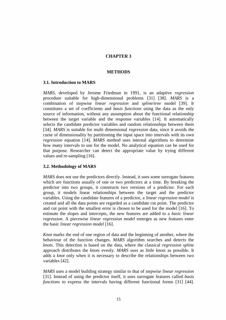
input space [41]. For an illustration we refer to Figure 1. If all predictor values are

distinct, the number of maximum basis functions is 2Np [31] [41].

Figure 1 An example of basis functions 0.5 and   0. 5x x

The form of MARS model is as follows [31]:

0

1

,M

m m

m

f X h X

where hm(X) represents a basis function included in C or a product of more than

one such functions and βm are estimated coefficients by minimizing RSS through

linear regression [31].

Afterwards, products of basis functions can be added to the model as well. The

form of such terms can be represented as [31]:

1 2  

ˆ ˆ ,a j a jm mh X X t h X t X

17

where ha(X) represents one of the reflected pairs that are considered to be added

to the model at that particular time [31].

MARS method is composed of a forward and a backward stage [42] [43]. The

forward stage aims to produce and basis functions, larger than optimal number to

deliberately overfit the training data [43]. The model starts by the constant

function 0  1h X [31]. Basis function pairs that give the largest RSS decrease in

the model are progressively and recursively added [39], until the model reaches a

user specified maximum basis functions [44]. Then, by backward stage MARS

eliminates basis functions, which contributes less to the training error [31] [39]

[42] selectively and iteratively one by one to choose the most generalizable

approximation [43]. This pruning process aims to limit the complexity of the

model by reducing the number of its basis functions, since like most of the

nonparametric methods, MARS is generally adaptive and flexible, which may

generate overfitting unless counteracting preventions are applied [14].

In data mining, the model quality is assessed usually by partitioning data into

training and test tests. However, when the data set is small, holding out a subset of

the data (usually, one-half to one-third of the data) may cause some representative

data to be excluded from the training set. In addition, performing testing on a

small data set may cause some sensitiveness to the random variation. Therefore

misleading goodness of fit results may occur. An alternative approach to assess

how well the model will predict unseen objects is cross validation [40]. In fact, the

balance between the accuracy and complexity of the model is achieved by an

index, called Generalized Cross Validation (GCV) [39]. GCV is an approximation

to the cross validation term, which averages a weighted prediction error over the

entire data set by using each data point as the testing set [40]. To determine the

contribution of the features on the model performance, how much the error rate is

decreased when each predictor variable is added into the model is estimated. GCV

statistics is used for this purpose. GCV produces a refined error estimate rather

than the apparent error rate. By default, the number of terms to remove is

automatically determined using GCV [16]. MARS finds the optimal model, using

the GCV value. The optimal model chosen at the end of the backward pruning

process [31]. It is the one with the lowest GCV measure [31] [40]:

2

1

2

ˆ( ( ))( ) :

(1 ( ) / ),

N

i iiy f x

GCVM N

where ( )M represents the effective parameters, which is the summation of the

number of term used in the model and the number of parameters used to estimate

the knot places in the model [31]. The degree of features added to the model and

the number of retained terms constitute the tuning parameters of the MARS model

[16].

18

MARS has several advantages including automatic feature selection [16], being

able to perform rapidly [43]. It does not require much pre-processing such as

predictor filtering or data transformations [16]. It can handle multi-valued

categorical inputs and missing values naturally [38]. Correlated predictors can

complicate the model interpretation but do not affect model performance [16].

MARS can handle categorical variables, considering all possible binary

combinations of the categories as two different groups. These binary combinations

are used to create a pair of basis functions and treat it as any other [31].

Each basis function of MARS operates in a specific region of the predictor space,

constructs piecewise linear models for the local relationships and is set to zero out

of their localization [16] [31]. A useful option sets an upper limit on the order of

interaction. For instance, allowing at most two-way interactions eases the

interpretations remarkably [31]. When the upper limit of interactions are set to 1,

the model becomes additive and interprets clearly how each predictor relates

individually to the outcome without considering the other predictors [16] [31].

To try every candidate knot, for a predictor with N observations, linear

regression models with O(N) operations are needed to be performed. MARS

appears to use totally O(N2) operations, but it does not. It starts trying the

rightmost candidate knot and move from right to left trying one knot at a time. In

each move, the basis functions differ by a constant over the right part, by zero

over the left part. Therefore, after each move the fit is updates O(1) times and

MARS uses totally O(N) operations [31].

Smoothing or complexity of a model in MARS can be determined by the number

of basis functions [31]. As the model becomes more complex, the variance tends

to increase as well where the squared bias tends to decrease [31]. As model

complexity increases, the training error decreases but as the training error

becomes too small, the generalization ability decreases, and the model becomes

overfit to the training data [31]. The generalization performance of a learning

method is a measure of its prediction capability on test data and the quality of the

model [31].

The modeler can set some parameters of MARS, to investigate different models, in

order to find the optimal model. One of the major parameters is the maximum

basis functions [40] [45]. Each iteration of forward step adds 2 basis functions to

the model. Therefore, this setting also specifies the number of forward steps

MARS will iterate [45]. The optimum maximum number of basis functions mainly

on the data size. For larger data sizes, it should be greater. By default, it is set to

15. The best way of detecting the optimal setting for maximum basis functions is

trial and error [40].

19

Another major parameter of MARS which the modeler can specify, is the

maximum interactions. By default it is set to 1, which does not consider any of the

interactions between the predictors. It is called main effect model. However, the

main affect model may not constitute a good fit to the data. The optimal setting

should also be detected by trial and error approach. If the GCV value of the model

decreases when the interactions are allowed, then that model should be preferred.

If there is no improvement in GCV value, the interactions should not be included.

To obtain an optimal model, MARS favours adding new variables. However, there

is a parameter, penalty on added variables, which can be modified by the

modeler, to exclude highly correlated variables from the model [40].

The parameter, minimum observations between knots, is set to 0 by default. It can

be set to a positive integer, but if it is not altered, MARS automatically handles it,

considering the sample size and model complexity. If the modeler sets it to 1,

MARS becomes more locally adaptive, since it considers a knot at any value [45].

3.3. Application of Multiple Linear Regression and MARS on the Real World

Data Set

3.3.1. Data Collection Procedure

The dietary intervention and clinical analysis of DIOGenes [13] was composed of

two research periods; low calorie diet (LCD) and dietary intervention. Initially,

932 volunteers (312 male and 620 female) from 891 families with at least one

obese or overweight parent (BMI≥27 kg/m2) attended a low-calorie diet for 8

weeks with the goal to lose at least 8% of their body weight. The volunteers

achieving that goal (773 volunteers) were randomized to 5 dietary groups: high

protein/high glycemic index (HP/HGI), low protein/low glycemic index (LP/LGI),

high protein/low glycemic index (HP/LGI), low protein/high glycemic index

(LP/HGI) as well as a control group, providing the measures of national dietary

guidelines. All diets were non-energy restricted (ad libitum) but low in fat (25–

30% of energy from fat). In one centre type (shopping centre), 263 volunteers

were given all food free, while in the other centre type 510 got dietary instructions

only. 548 volunteers managed to finish the dietary intervention period while the

others dropped out [13].

20

Figure 2 Schematic overview of DIOGenes [13]

There were three main investigation days of the study: pre-LCD (baseline), post-

LCD (randomization) and post-intervention (cf. Figure 2) [13].

3.3.2. Data Description and Pre-processing Details

Data set was composed of 7 variables: X1 (centre type), X2 (drop-out), X3 (dietary

GI), X4 (dietary protein), X5 (weight change), X6 (baseline HOMA-IR), and Y

(HOMA-IR change). We used X1, X2, X3, X4, X5, and X6 as predictors, and Y as the

target variable (Table 3). While X1, X2, X3 and X4 are categorical variables, X5 and

X6 and Y are continuous.

21

Table 3 The variables included in the data set

Y HOMA-IR change HOMA-IR change during dietary intervention

I0*G0/135 (SI units)

X1 Center type

center type:

1="not shopping center",

2="shopping center"

X2 Drop-out

drop-out:

0 = "no drop-out after the LCD",

1 = "drop-out after the LCD"

X3 Dietary GI pattern

low glycemic index diet:

0 = "no",

1 = "yes"

X4 Dietary protein pattern

high protein diet:

0 = "no",

1 = "yes"

X5 Weight change weight change during dietary intervention

X6 Baseline HOMA-IR HOMA-IR, calculated after low calorie diet

(before dietary intervention)

The labels for X3 are “1” and “0”. They reflect the low GI and high GI,

respectively. Similarly for, X4 labels “1” and “0” represent high protein and low

protein dietary patterns, respectively. X5 corresponds to weight change during

dietary intervention. During low calorie diet, the participants attended the same

commercially available diet. On the other hand, in different centre types there was

a difference regarding the application of dietary intervention. In shopping center

263 volunteers got all food free, while 510 volunteers, in the other type of

research centre, got dietary instructions only. Label 2 is used for shopping centre,

and 1 for the other centre type. Furthermore, X2 reflects withdraw or completion;

label 1 corresponds to drop-out while 0 corresponds to completion [13].

Since we used raw data, some pre-processing was needed before the model

construction. We followed the pre-processing procedure of a formerly published

study within the scope of DIOGenes [46]. We selected only the patients with the

most successful weight loss (at least 10% per cent of their initial weight) [13].

Missing values which are due to withdraw from the study are not considered as

randomly missing, since withdraw can be related to a lower adherence to the

particular diet type [13] [46]. Such missing values are assumed to be the same as

the value before dietary intervention [46]. Therefore, the changes of such values

(weight and HOMA-IR) during dietary intervention were recorded as 0 [13]. The

missing values except for the ones resulting from withdraw, assumed to be

missing at random. They are consequences of 3 facts: Some of the blood samples

22

got lost; some of them were in a small amount to perform the analysis and some

of the measurements were failed [46]. Such missing values are excluded from the

analysis.

Figure 3 Scatter plot matrix based on the data set after pre-processing

According to the scatter plot matrix (cf. Figure 3), the output values of the group 1

of X1 (center type) is more dispersed, whereas the output values of group 2 is

aggregated in a smaller area. It makes sense because patients in group 2 had the

food for free whereas the other group had dietary instructions only. It may have

caused some difference between the individuals.

Similarly, output values for the individuals in group 0 of X2 (drop-out) are more

dispersed, while the output values of group 1 are aggregated in a smaller area. It is

because we filled the missing values caused by drop out by 0.

For the output values for the individuals in group 1 of both X3 (low glycemic

index) and X4 (high protein content) are marginally dispersed. On the contrary, the

output values for the individuals in group 0 of each variable are gathered in a

small interval.

23

The values of X5 and X6 (weight change and baseline HOMA-IR value,

respectively), but their Y values are close, except of some dispersal.

3.3.3. Application of Multiple Linear Regression

Initially, we performed multiple linear regression using all of the predictors.

Afterwards, we conducted multiple linear models excluding first dietary protein

content, then glycemic index variables.

3.3.4. Application of MARS

First, we included all the variables to the model and adjusted the maximum

interactions by trial and error (restricting by 1, 2, 3, 4 and then 5, respectively),

and maximum basis functions. We left the other parameters as default. We found

the optimal model considering the GCV value.

3.3.5. Initial Models

Using all the variables, we observed the optimal models for different level of

maximum interactions. Initially, we used the default setting for maximum

interactions, 1, to observe the main models. Then, enhancing the maximum

interactions by 1 in each iteration we observed the GCV values of each optimal

model, for corresponding settings.

Since none of the first optimal models included X3, we excluded X3 and repeated

the same procedure.

3.3.6. Observing How MARS Parameters Affect the Model Performance

To illustrate the effect of maximum basis functions on the model performance, we

started with the default setting of maximum basis functions, 15, and increased the

setting by 5, in each application. We limited maximum interactions by 2, and left

all the other parameters as default. We observed both adjusted-R2 and GCV values

of the optimal models.

To achieve a clearer interpretation, we limited the maximum interactions by 2.

Changing the minimum observations between knots parameter, and adjusting the

maximum basis functions, we observed how the performance of the optimal model

alters.

24

25

CHAPTER 4

RESULTS

4.1. Multiple Linear Regression

Multiple linear regression model we achieved when we used all the predictors had

an adjusted-R2

of 0.026 and an R2

value of 0.056. The adjusted-R2

value of the

multiple linear model we constructed without using protein content as a predictor

was 0.030, and the R2 value was 0.055. The adjusted-R

2 value of the multiple

linear model we constructed without using glycemic index as a predictor was

0.031, and the R2

value was 0.055. There are only slight differences between the

adjusted-R2

values of those models (see Appendix C).

Formerly, Goyenechea et al. performed multiple linear regression to the data [13].

The multiple linear regression models excluding glycemic index and protein

content dietary patterns has R2 values of 0.14, and 0.17, respectively [13].

Performances of the linear models which we conducted are different than that of

the model formerly conducted, because of the differences in data pre-processing.

4.2. Performance of the Initial MARS Models and the Effect of Maximum

Interactions on the Performance of Optimal Models

We detected the optimal models for each maximum interaction setting, by trying

different maximum basis functions. As we increased maximum interactions, GCV

values tended to decrease, while naive and adjusted-R2 values tended to increase,

except of a reverse tendency when maximum interactions increased to 4. We

found the optimal model with the lowest GCV value, when we set maximum

interactions to 5, and maximum basis functions to 53, It had a GCV value of 0.58,

an adjusted-R2 value of 0.78, and an R

2 value of 0.79 (cf. Table 4).

Table 4 Optimal models for different maximum interaction settings

Maximum

interactions

Maximum

number of

basis functions

R2

Adjusted-

R2 GCV

Variables

appeared in

the final model

no

interactions 20 0.15 0.13 1.84 X5, X6

2-ways 55 0.71 0.61 0.92 X5, X6

3-ways 76 0.75 0.74 0.77 X2, X4, X5, X6

4-ways 55 0.65 0.63 1.02 X2, X5, X6

5-ways 53 0.79* 0.78 0.58 X1, X2, X4, X5,

X6

26

The predictor variable X1 appeared only when maximum 5-way interactions are

allowed. Furthermore, X3 (dietary glycemic index) did not appear in any of the

models (cf. Table 4), which means it does not have any contribution to the model.

All the other variables appeared at least in one of the optimal models. Therefore,

we took X3 out and repeated the same procedure.

4.3. Optimal Models for Dietary Protein

Excluding the X3 variable, we observed the final models, following the same

steps. Again, for each maximum interactions level, we detected optimal models by

changing maximum basis functions. The model with the lowest GCV value, and

the highest R2

value emerged, when we set the maximum interactions parameter to

5 and adjusted the maximum basis functions parameter by trial and error. Table 5

shows the performance of optimal models for different maximum interactions.

When we allowed interactions, the adjusted-R2

values of the optimal models

tended to improve.

Table 5 The performance of optimal models for dietary protein for different

maximum interactions settings

Maximum

interactions

Maximum

number of

basis

functions

R2

Adjusted-

R2 GCV

Variables

appeared in the

final model

no interactions 20 0.15 0.13 1.84 X5, X6

2-ways 37 0.53 0.51 1.18 X5, X6

3-ways 54 0.78 0.76 0.86 X2, X5,X6

4-ways 75 0.81 0.79 1.22 X1, X2, X4, X5, X6

5-ways 65 0.84 0.82 0.80* X1, X2, X4, X5, X6

As we enhanced maximum interactions, R2

and adjusted-R2

values of optimal

models increased steadily. Similarly, GCV values for optimal models showed a

propensity decrease, but, increased by maximum interactions of 4. We observed

the model with the best performance among the optimal models, when we set the

maximum interactions to 5 (cf. Table 5). It had a GCV value of 0.80, R2 value of

0.84, and adjusted-R2 value of 0.82. The performance of the final model, had a

higher R2 value than the one we observed, in Section 4.2. However, it has a lower

GCV value. It is probably because of the presence of irrelevant data objects, which

reduce model performance.

Our final model equation consists of 20 basis functions. The model equation of the

best model we achieved is as follows:

27

4 7

9 11

17 20

22

( ) ( )

( ) ( )

0.00760097 0.737043 0.334955

 0.277449 0.10171

1.3086 2.12107

0.741

61

( )

9

( )

( )

h X h X

h X h X

h X X

X

Y

h

h 23

37 41

43 47

49 51

1  .94626

4.47154 0.960445

   2.83687 0.0827298

0.297437 0.306253

( )

( ) ( )

( ) ( )

( ) ( )

h X

h X h X

h X h X

h X h X

52 56

57 58

60 62

0.24663 0.269962

0.158291

( ) ( )

( ) ( )

  0.981747

0.649299 ( ) 0.198785 ( ).

h X h X

h X h X

h X h X

The basis functions used by MARS model are:

51 max 0( ) ,, 29.5h XX

53 max 0, 11( ) ,h X X

64 3max 0, 0.565889( ) ( ),h X h XX

55 max 0,( ) ,0Xh X

56 max 0,0 ,( )h X X

67 6max 0, 1.74775( ) ( ),h X h XX

29 1 ( ) ( ),"0"X inh X h X

611 9( ) ( )max 0, 1.20256 ,Xh X h X

17 54( ) ( ) 1" ,"X inh X h X

18 54( ) ( ) 0" ,"X inh X h X

520 max 0,( ,9) Xh X

521 max 0,9( ) ,h X X

622 20 max 0, 0.56( ) ( ),5889h hXX X

523 max 7) ,0, .4( Xh X

427 21 "1" ,( ) ( )X inh X h X

630 27max 0,4.28 ( )321( ) ,Xh X h X

632 27max 0, 3.1( ) ( )6821 ,Xh X h X

634 27max 0,3.75( ) ( )6 ,86 Xh X h X

237 34 ( ) ( ),"0"X inh X h X

28

640 27 max 0, 2.4998( ,1) = ( )Xh X h X

241 40 ( ) ( ),"0"X inh X h X

243 30 ( ) ( ),"0"X inh X h X

146 34 ( ) ( ),"1"X inh X h X

247 46 ( ) ( ),"0"X inh X h X

649 9max 0, 3( ) . )2 ( ,7198h XX h X

651 18max 0, 0.56588( ) ( ),9h X h XX

52 9

54 9

55 9

4

56 5

6

4

56

max 0, 3.12628

( ) ( ),

( ) ( ),

(

"1"

"0"

max 0,

) ( ),

( ) (2.75 8 ,4 5 )

h X h X

h X h X

h X

X

X in

X i

h

n h

XX

X

X h

6

2

6

57 55

58 32

60 5

6 5462

( ) ( ),

( ) ( ),

(

max 0, 2.75485

"0"

max 0, 2.2) (777

max 0, 1.747

),

( ) ( ).75

h X h X

h X h X

h X h X

X

X

h X

n

h

X

X X

i

Basis function equations can also be written as follows to see the interactions

between the variables more clearly:

64 5max 0, 0.565889 max 0, 1 ,( ) 1h X X X

67 5max 0, 1.74775 max 0 ,( ) , 0X Xh X

29 5 "0" max 0, 2 . ,( ) 9 5X in Xh X

611 2 5max 0, 1.20256 "0" max 0, 29.5) ,( X X in Xh X

29

17

20

22

23

37

4 5

5

6 5

5

2 6 4 5

2 6 441 5

"1" max 0, 0 ,

max 0, 9 ,

 max 0, 0.565889 max 0, 9 ,

max 0, 7.4 ,

"0" max 0,3.75686 "1" max 0,9 ,

"0" max 0, 2.49981 "1" m

( )

( )

( )

( )

ax

( )

0,( ) 9

X in X

X

X X

X

X

h X

h X

h X

h X

in X X in X

X in X X i X

h

n

X

h X

43

47

2 6 4 5

2 1 6 4

5

,

"0" max 0, 3.16821 "1" max 0,9 ,

"0" "1" max 0,3.756

( )

( )

86 "1"

max 0,9 ,

X in X X in X

X in X in X X in

X

h X

h X

649 2 5max 0, 3.71982 "0" max 0, 2( 5) 9. ,XX Xh in X

651 4 5max 0, 0.565889 "0" max 0, 0 ,( )h X X X in X

652 2 5max 0, 3.12628 "0" max 0, 29.5) ,( X X in Xh X

656 4 2 5max 0, 2.75485 "0" "0" max 0, 29.5 ,( ) X X inh X in XX

6 27 45 5max 0,2.75485 "0" "0" max 0, 29.5 ,( ) X X inh X in XX

258 6 4 5 "0" max 0, 3.168( ) 21 "1" max 0,9 ,X in X X in Xh X

660 5max 0, 2.2777 max 0, 0 ,( ) Xh X X

662 4 2 5max 0, 1.74775 "1" "0" max 0, 29.5 .( ) X X inh X iX n X

Basis functions 20 and 23 are related to X5, directly. Basis functions 4, 7, 22 and

60 are related to X6 directly and X5 indirectly. Basis function 9 is directly related

to subset 1 of X2, indirectly to X5. Basis function 17 is directly related to subset1

of X4 and indirectly to X5. Basis functions 11, 49, 52 and are related to the

variables X2, X5 and X6. Basis function 51 is related to the variables X4, X5, X6.

Basis function 47 is related to X1, X3, X4, X5, and X6. Remaining 7 basis functions

are related to subset 0 in X2, X6, Subset 1 of X4 and X5.

Table 6 represents the coefficients of the basis functions which are extracted from

the model equation.

30

Table 6 The coefficients of the basis functions appeared in the optimal model

Basis function Coefficients

0 0.0076

4 0.7370

7 -0.3350

9 0.2774

11 -0.1017

17 -1.3086

20 -2.1211

22 0.7416

23 1.9463

37 4.4715

41 -0.9604

43 -2.8369

47 0.0827

49 -0.2974

51 -0.3063

52 0.2466

56 0.2700

57 -0.1583

58 -0.9817

60 -0.6493

62 0.1988

31

Table 7 illustrates the variables or groups of interacting variables which affect the

model performance. Here, X5 can be considered as the most important variable,

because it appears in every basis function included in the model equation. The

interacting affects are between: X5 and X6; X2 and X5; X4 and X5; X2, X5, and X6;

X4, X5, and X6; X2, X4, X5, and X6; X1, X2, X4, X5, and X6. According to the cost of

emission values, the interaction effects from most important to less important are

between the variables X2, X4, X5, and X6; X4 and X5; X2 and X5; X5 and X6; X1, X2,

X4, X5, X6; X4, X5, and X6; X2, X5, and X6, respectively.

Table 7 Cost of omission, the number of basis functions and variables related to

each function of the model

Function Cost of omission No of basis

functions Variables

1 0.88084 2 X5

2 1.10663 4 X5, X6

3 1.13789 1 X2, X5

4 1.18222 1 X4, X5

5 0.95453 3 X2, X5, X6

6 1.01270 1 X4, X5, X6

7 2.69535 7 X2, X4, X5, X6

8 1.02422 1 X1, X2, X4, X5, X6

We conducted the model again by randomly selecting 20% of the data for testing.

The model performance (adjusted-R2 and R

2 values) decreased dramatically.

4.4. The Effect of Maximum Basis Functions and Minimum Observations

between Knots on Model Performance

Until now, we observed the performance of the optimal model for each possible

maximum interaction setting, by adjusting maximum basis functions. To illustrate

the individual effect of maximum basis functions, we used a fixed value of 2 for

maximum interactions and left the other parameters as default. Figure 4 illustrates

how the adjusted-R2

and GCV values change, as we set the maximum basis

functions to greater values. As the maximum basis functions increase from 15 to

40, we observed an important improvement in the model performance. At 40, we

observed the optimal model for these settings, with the lowest GCV value (1.18).

32

Between the maximum basis functions settings 40 and 50, the GCV value

decreased slightly and remained constant for larger values. The adjusted-R2 values

tended to rise, by the increase of maximum basis functions. After reaching a peak

at maximum basis functions settings of 50, it showed a slight decline and remained

constant for larger settings.

Figure 4 The effect of maximum basis functions change on the adjusted-R

2 and

GCV values

So far, we performed MARS changing only the maximum interactions and

maximum basis functions settings. We found the optimal model when we allowed

5-way maximum interactions.

To achieve a clearer interpretation, we limited the interactions by 2. Adjusting the

minimum observations between knots, we observed how the performance of the

model alters.

Table 8 represents the optimal models we observed when we changed the settings

of minimum observations between knots. We achieved the optimal model with the

lowest GCV value, when we set minimum observations between knots to 1. It had

an R2 value of 0.96, adjusted-R

2 value of 0.96 and GCV value of 0.30.

0,00

0,20

0,40

0,60

0,80

1,00

1,20

1,40

1,60

1,80

2,00

152025303540455055606570758085maximum basis

funcitons

Adjusted R Squared

GCV

33

Table 8 Optimal models for dietary protein when maximum interactions are

limited by 2

Min. obs. between knots Max. basis functions R2

Adjusted-R2 GCV

0 (default) 40 0.53 0.51 1.18

1 60 0.96* 0.95 0.30*

2 85 0.92 0.91 0.56

3 70 0.75 0.73 0.89

4 60 0.68 0.66 1.10

5 65 0.50 0.45 1.50

6 40 0.63 0.61 0.93

7 95 0.61 0.59 1.03

8 45 0.63 0.61 1.02

9 80 0.73 0.71 1.10

10 30 0.50 0.48 1.43

15 65 0.61 0.59 1.30

20 55 0.36 0.33 1.83

4.5. The Optimal Model with Testing

So far, we used the whole data set as training set. To avoid overfitting, we used

0.20 of the data for random testing. We set the maximum interactions to 2 again

to achieve a clearer interpretation. Changing the other MARS parameters

(minimum observations between knots, maximum number of basis functions and

speed) we observed various models. We observed the final model when we set the

maximum number of basis functions to 45, speed parameter to 5, and minimum

observations between knots to 1.

The backward stage ended up with a model containing piecewise 5 basis functions.

These basis functions are combined and related to only 3 of the variables: X4, X5, and X6

(protein content, weight change and baseline HOMA-IR value). In other words,

only those three predictors had a contribution to the performance of the model.

The basis functions, remained at the end of backward pruning procedure, are

illustrated below:

52 max 0, 11( ) ,h X X

5 6 2( ) max{0, 3.95351} ( )  ,h X X h X

69 2  max 0, 4.09755( ) ( ),h X hX X

619 2max 0, 3( ) . )8 ( ,1262h XX h X

524 max 0, 9.4) ,(h X X

427 24  ( ) ( ). "1"X inh X h X

34

To see the interactions between the predictors, may also be written as:

52 max 0, 11( ) ,h X X

6 55 ( ) max{0, 3.95  max 0, 11 ,351}h X X X

6 59  max 0, 4.09755 max 0,( ) ,11XX Xh

619 5max 0, 3.12628 max 0, ,11( )h X X X

524 max 0, 9.4) ,(h X X

427 24  ( ) ( ). "1"X inh X h X

The final model equation is as follows:

5 9 19

27

( ) ( )  0.090307 15.7047 13.47 2.30274

0.0168057

( )

( ) .

h X h X h X

h

Y

X

Can also be written as:

6 5

6 5

6 5

4 5

  0.090307 15.7047   max 0, 11

13.47  max 0, 4.09755 max 0, 11

2.30274 max 0, 3.12628 max 0, 11

0.0168057   "1" max 0, 9.4

max{0, 3.95351}

.

Y X

X X

X X

X in X

X

Table 9 represents the coefficients of basis functions which are extracted from the

model equation, and variables related to each basis function either directly or

through another basis function. All the basis functions appeared in the final model

equation are related to X5 directly or indirectly. Also X6 showed relatedness with

most of the basis functions. Some basis functions are linked to X6 and X5 or X4 and

X5. However, X4 and X6 did not appear together in a basis function.

Some coefficients of basis functions related to X5 were remarkably high.

Moreover, X6 and X5 were highly interacting with each other, and they had a

strong combined effect on the model performance. We also observed an

interaction between X6 and X4. The variables X1, X2, and X3 did not appear in the

final model.

35

Table 9 Coefficients of each basis function appeared in the model equation

Basis Function Coefficients

0 0,0903

5 15,7047

9 -13,4700

19 -2,3027

27 -0,0168

4.6. Comparing the Performance of MARS Models with the Performance of

Multiple Linear Regression Model

We compared the performances of the optimal MARS model we achieved after

doing the adjustments, and the optimal MARS model we achieved when we did

testing with the multiple linear model which we conducted.

Since the variable glycemic index did not appear in any of the MARS models, we

compared the performance of the models we conducted excluding glycemic index.

Table 10 illustrates the adjusted-R2 values of each model. The adjusted-R

2 value

of multiple linear model, 0.03, is absolutely lower than that of the optimal MARS

model (0.82). When we conducted MARS models by separating 20 % of the data

for random testing, the adjusted-R2 values decreased remarkably. Doing the

adjustments, we managed to find an optimal model with testing.

Table 10 Multiple linear regression model versus MARS models

Model Adjusted-R2

Multiple Linear Regression model 0.031

Optimal MARS model 0.82

Optimal MARS model with testing 0.67

36

37

CHAPTER 5

CONCLUSION AND OUTLOOK

We used the clinical data from the DIOGenes research project. One of the

objectives of this study was to use MARS to detect if dietary protein and glycemic

index patterns and/or other predictors we selected were related to insulin

resistance change. Moreover, we aimed to observe the performance of MARS

model on the current data. We wanted to find out if MARS constitutes a good

approximation for it. Adjusting the parameters, we observed how the performance

of MARS changes, and thereby we tried to find a good prediction for our problem.

Formerly, in the concept of DIOGenes, Goyenechea et al. [13] performed a

multiple linear regression analysis to observe the relationship between the

different dietary patterns regarding the macronutrient content, i.e., dietary protein

and glycemic index patterns and insulin resistance change. We aimed to find a

model which constitutes a better approximation to the data.

After preparing the data set, we performed multiple linear regression to the same

data. The model performance was different than that of Goyenechea et al., due to

differences in the pre-processing procedure.

We observed that multiple linear models do not perform well on our data. We

constructed a MARS model, first including all the variables. We observed the

optimal models for different maximum interactions and maximum basis functions.

We left all the other settings as default. We ended up with models having better

performance on the data compared to multiple linear regression. We observed the

optimal model with the best performance when we allowed the consideration of 5-

way interactions between predictors. Weight change, dietary protein, baseline

insulin resistance, center type and drop-out had an effect on the final model.

However, dietary glycemix index did not appear in any of the results. Therefore,

we could not observe the effect of it on the model performance.

We repeated the same procedure again but this time, we excluded dietary

glycemic index from the data set. We achieved a better performance than our

previous model.

According to our results, there was no link between dietary glycemic index and

insulin resistance change. However, we managed to detect a relationship between

weight change, dietary protein, baseline insulin resistance and insulin resistance

change. Center type did not have a direct effect on the model performance.

However, this variable was interacting with the other variables in the model.

38

Considering our optimal model without testing, drop-out, dietary protein content,

and weight change was strongly related to insulin resistance change. Moreover,

protein content and weight change were interacting with each other and they had a

strong combined effect on the model performance. We also observed an

interaction between drop-out and weight loss as well as between weight change

and baseline insulin resistance. Centre type had an indirect effect o the model

performance, occurred as a 5-way interaction with the other predictors.

So far, we used the whole data set as training set. To avoid overfitting, we used

0.20 of the data for random testing. However, the model performance was not as

efficient as was expected.

To find a simpler model, we limited the maximum interactions by 2-ways, and to

detect local relationships more accurately, we adjusted MARS parameters for a

more intense search through the data points. Compared to our first models with

testing, we ended up with an optimal model which fits the data better and provides

a clearer interpretation.

Only, protein content, weight change and baseline insulin resistance appeared in

the final model. In other words, only those three predictors had a contribution to

the performance of the model.

There was an interaction between weight change and baseline insulin resistance

and they had an important effect on the model performance. Similarly, weight

change and protein content was interacting with each other. Drop-out did not

appear in the final model. This may be because the individuals who completed

dietary intervention had a variety of insulin resistance change values, although

there was only one value for the withdraw group. This may have caused some

noise and it may be the underlying reason why drop-out variable did not appear in

the final model. Similarly, our final model with testing did not indicate any

relationship between center type and insulin resistance. In other words, according

to the model, applying the dietary intervention either by food supplement or by

dietary instructions did not make an observable difference. Also, the absence of

these two predictors in the final model means neither center type nor drop-out

affected the performance of the model for the current settings.

Considering our observations, we conclude that scientific researches, investigating

new prevention approaches to type 2 diabetes should take into account weight

change and dietary protein patterns. They should also take baseline insulin

resistance values into consideration.

MARS is a nonlinear, model based method, which can detect interactions between

the variables [45]. It uses a trade off between stability and accuracy [39].

Alternative varieties of MARS exist (CMARS, RMARS, etc.) [41].

39

Future studies could focus on the use of further emerging optimization-supported

data mining tools, such as CMARS and RMARS [41], and the comparison of their

results with the results of this thesis.

40

REFERENCES

[1] World Health Organization Fact Sheet No: 311: Obesity and overweight.

Retrieved January 11, 2014, from

http://www.who.int/mediacentre/factsheets/fs311/en/index.html.

[2] Kazaks, A., & Stern, J. S. (2013). Nutrition and Obesity: Assessment,

Management & Prevention. (11, 55). Burlington, MA: Jones & Bartlett

Publishers.

[3] Astrup, A., & Pedersen, S. (2010). Obesity. In Geissler, C., & Powers, H. J.

(Ed.). Human nutrition. (402-424). New York: Elsevier Health Sciences.

[4] Riccardi, G., Capaldo, B., & Rivellese A. A. (2010). Diabetes Mellitus. In

Geissler, C., & Powers, H. J. (Ed.). Human nutrition. (425-438). New York:

Elsevier Health Sciences.

[5] Kearney, J., & Geissler, C. (2010). Food and nutrient patterns. In Geissler, C.,

& Powers, H. J. (Ed.). Human nutrition. (8). New York: Elsevier Health Sciences.

[6] Aldrich, N. D., Perry, C., Thomas, W., Raatz, S. K., & Reicks, M. (2013).

Perceived importance of dietary protein to prevent weight gain: a national survey

among midlife women. Journal of nutrition education and behavior, 45(3), 213-

221.

[7] Solomon, T. P., Haus, J. M., Kelly, K. R., Cook, M. D., Filion, J., Rocco, M.,

Kashyap S. R., Watanabe R. M., Barkoukis H., & Kirwan, J. P. (2010). A low–

glycemic index diet combined with exercise reduces insulin resistance,

postprandial hyperinsulinemia, and glucose-dependent insulinotropic polypeptide

responses in obese, pre diabetic humans. The American journal of clinical

nutrition, 92(6), 1359-1368.

[8] Westerterp-Plantenga, M. S., Luscombe-Marsh, N., Lejeune, M. P., Diepvens,

K., Nieuwenhuizen, A., Engelen, M. P. K. J., Deutz, N. E. P., Azzout-Marniche,

D., Tome, D., & Westerterp, K. R. (2006). Dietary protein, metabolism, and body-

41

weight regulation: dose–response effects. International Journal of Obesity, 30,

16-23.

[9] Lau, C., Færch, K., Glümer, C., Tetens, I., Pedersen, O., Carstensen, B.,

Jørgensen, T., & Borch-Johnsen, K. (2005). Dietary Glycemic Index, Glycemic

Load, Fiber, Simple Sugars, and Insulin Resistance The Inter 99 study. Diabetes

care, 28(6), 1397-1403.

[10] Bonora, E ., Targher G., Alberiche, M., Bonadonna, R. C., Saggiani, F.,

Zenere, M. B., Monauni, T., & Muggeo, M. (2000). Homeostasis model

assessment closely mirrors the glucose clamp technique in the assessment of

insulin sensitivity: studies in subjects with various degrees of glucose tolerance

and insulin sensitivity. Diabetes care, 23(1), 57-63.

[11] Trout, K. K., Homko, C., & Tkacs, N. C. (2007). Methods of measuring

insulin sensitivity. Biological Research for Nursing, 8(4), 305-318.

[12] Larsen, T. M., Dalskov, S., van Baak, M., Jebb, S., Kafatos, A., Pfeiffer, A,

Martinez, J.A., Handjieva-Darlenska, T., Kunesová, M., Holst, C., Saris,

W.H.,Astrup, A.( 2010) The Diet, Obesity and Genes (Diogenes) Dietary Study in

eight European countries - a comprehensive design for long-term intervention.

Obes Rev. 11(1), 76-91.

[13] Goyenechea, E., Holst, C., van Baak, M. A., Saris, W. H., Jebb, S., Kafatos,

A., Pfeiffer, A., Handjiev, S., Hlavaty, P., Stender, S., Larsen, T. M., Astrup, A.,

& Martinez, J. A. (2011). Effects of different protein content and glycaemic index

of ad libitum diets on diabetes risk factors in overweight adults: the DIOGenes

multicentre, randomized, dietary intervention trial. Diabetes/Metabolism Research

and Reviews, 27(7), 705-716.

[14] Statsoft, Inc. (2013). Electronic Statistics Textbook. Tulsa, OK: Statsoft.

WEB: http://www.statsoft.com/textbook/.

[15] Takezawa, K. (2006). Introduction to nonparametric regression. Hoboken,

N.J. : Wiley- Hoboken.

[16] Kuhn, M., Johnson, K. (2013). Applied Predictive Modeling. New York:

Springer.

42

[17] National Institute of Diabetes and Digestive and Kidney Diseases. Insulin

Resistance and Prediabetes. National Diabetes Information Clearinghouse.

Retrieved July 04, 2013, from

http://diabetes.niddk.nih.gov/dm/pubs/insulinresistance/#what; 2012.

[18] Unger, J. (2012). Pathogenesis of Type 2 Diabetes- A Comprehensive

Analysis. In Bagchi, D., & Sreejayan, N. (Ed.). Nutritional and therapeutic

interventions for diabetes and metabolic syndrome. (29-41). San Diego USA:

Elsevier.

[19] Sieri, S., Krogh, V., Berrino, F., Evangelista, A., Agnoli, C., Brighenti, F.,

Pellegrini N, Palli, D., Masala, G., Sacerdote, C., Veglia, F., Tumino, R., Frasca,

G., Grioni, S., Singh, B., & Saxena, A. (2010). Surrogate markers of insulin

resistance: A review. World journal of diabetes, 1(2), 36.

[20] Rao, G. (2001). Insulin resistance syndrome. American Family

Physician, 63(6), 1159.

[21] Risérus, U., Ärnlöv, J., Brismar, K., Zethelius, B., Berglund, L., Vessby, B.

(2004). Sagittal abdominal diameter is a strong anthropometric marker of insulin

resistance and hyperproinsulinemia in obese men. Diabetes Care, 27(8), 2041-

2046.

[22] Gupta K. A., Menon, A., Brashear, M., Johnson, W. D. (2012) Prediabetes:

Prevalence, Pathogenesis, and Recognition of Enhanced Risk. In Bagchi, D., &

Sreejayan, N. (Ed.). Nutritional and therapeutic interventions for diabetes and

metabolic syndrome. (57- 75) San Diego USA: Elsevier.

[23] National Institute of Diabetes and Digestive and Kidney Diseases. National

Diabetes Statistics. National Diabetes Information Clearinghouse. Retrieved June

25, 2013, from http://diabetes. niddk.nih.gov/dm/pubs/statistics/; 2011.

[24] American Diabetes Association. (2013). Diagnosis and classification of

diabetes mellitus. Diabetes Care, 36(1), 67-S74.

43

[25] American Diabetes Association (2013). Standards of medical care in

diabetes. Diabetes Care, 2013. 36(1), 11-66.

[26] National Institute of Diabetes and Digestive and Kidney Diseases. Diagnosis

of Diabetes and Prediabetes. (2012) National Diabetes Information

Clearinghouse. Retrieved June 28, 2013, from

http://diabetes.niddk.nih.gov/dm/pubs/diagnosis/.

[27] World Health Organization. (2009). Fact sheet No. 312: Diabetes. Geneva:

WHO. Retrieved June 25, 2013, from

http://www.who.int/mediacentre/factsheets/fs312/en/.

[28] World Health Organization. (1999). Definition, diagnosis and classification

of diabetes mellitus and its complications: report of a WHO consultation. Geneva:

World Health Organization.

[29] Matthews, D. R., Hosker, J. P., Rudenski, A. S., Naylor, B. A., Treacher, D.

F., & Turner, R. C. (1985). Homeostasis model assessment: insulin resistance and

β-cell function from fasting plasma glucose and insulin concentrations in

man. Diabetologia, 28(7), 412-419.

[30] Moszczynski, P., & Rutowski, J., A. (2012). Meal Plans for Diabetics:

Caloric Intake, Calorie Counting, and Glycemic Index. Nutritional and

therapeutic interventions for diabetes and metabolic syndrome. (431-442) San

Diego USA: Elsevier.

[31] Hastie, T., Tibshirani, R., & Friedman, J. (2009). The elements of statistical

learning: data mining, inference, and prediction. (321-334). New York: Springer.

[32] Dietterich, T. (1995). Overfitting and under computing in machine

learning. ACM computing surveys (CSUR), 27(3), 326-327.

[33] Hinton, P., Brownlow, C., & McMurray, I. (2004). SPSS explained. United

States, East Sussex: Routledge.

44

[34] Osei-Bryson, K. M. (2014). Overview on Multivariate Adaptive Regression

Splines. In Advances in Research Methods for Information Systems Research (93-

107). Springer US.

[35] Bates, D. M., & Watts, D. G. (1988). Nonlinear regression analysis and its

applications. (1-5). New York: Wiley.

[36] Montgomery, D. C., Runger, G. C., & Hubele, N. F. (2001). Engineering

statistics (298-309). New York: Wiley.

[37] Chen, W. K. (Ed.). (2009). Feedback, nonlinear, and distributed circuits. (9–

20). Boca Raton, FL : CRC Press.

[38] Friedman, J. H. (1991). Multivariate adaptive regression splines. The Annals

of Statistics, (19) 1-67.

[39] Wakefield, J. (2013). Bayesian and frequentist regression methods. ( 620-

630). New York: Springer.

[40] Meullenet, J. F., Xiong, R., & Findlay, C. J. (2007). Multidimensional

scaling and unfolding and the application of probabilistic unfolding to model

preference data. (179-205). Ames, Iowa, USA: Blackwell Publishing.

[41] Özmen A., & Weber G.-W. (2014). RMARS: Robustification of multivariate

adaptive regression spline under polyhedral uncertainty. Journal of

Computational and Applied Mathematics. 259 (2014) 914–924.

[42] Weber G.-W., Çavuşoğlu Z. Özmen A. (2012) Predicting default

probabilities in emerging markets by new conic generalized partial linear models

and their optimization, Optimization: A Journal of Mathematical Programming

and Operations Research, 61:4, 443-457.

[43] Friedman, J. H. (1993). Fast MARS, Department of Statistics. Stanford

University, Tech. Report LCS110.

45

[44] Özmen A. Kropat E., Weber G.-W. (2014). Spline regression models for

complex multi-modal regulatory networks, Optimization Methods and Software,

29:3, 515-534.

[45] SPM Users Guide. Introducing MARS This guide provides a brief

introduction to MARS. Retrieved January 04, 2014, from

http://media.salford-systems.com/pdf/spm7/IntroMARS.pdf.

[46] Gögebakan, Ö., Kohl, A., Osterhoff, M. A., van Baak, M. A., Jebb, S. A.,

Papadaki, A., Martinez J. A. , Handjieva-Darlenska, T. H., Hlavaty, P., Weickert,

M. O., Holst, C., Saris, W. H.M., Astrup, A., Pfeiffer, A. F. (2011). Effects of

Weight Loss and Long-Term Weight Maintenance with Diets Varying in Protein

and Glycemic Index on Cardiovascular Risk Factors. Clinical Perspective The

Diet, Obesity, and Genes (DIOGenes) Study: A Randomized, Controlled

Trial. Circulation, 124 (25), 2829-2838.

46

APPENDIX A

DIOGENES PROJECT EXCLUSION CRITERIA FOR SUBJECTS

Subject Exclusion criteria

Generally healthy

psychiatric diseases

eating disorders

infectious or inflammatory diseases

untreated hypo- or hyperthyroidism gastrointestinal,

liver or kidney diseases cardiac diseases

type 1 or type 2 diabetes mellitus

cancer within the last 10 years

food allergies

blood pressure ≥ 160/100 mmHg

blood triglycerides > 3 mM

blood total cholesterol > 7 mM

fasting blood glucose ≥ 6.1 mM

urinary protein, glucose, pH, ketone and hemoglobin

outside accepted reference ranges

use of prescription medication

alcohol consumption > 21 alcohol units/week (males),

> 14 units/week (females)

planned major changes in physical activity during the

study period

blood donation within the past 2 months

weight change > 3 kg in the 3 months prior to the

study

participation in another scientific study up to 3

months before

drug treatment,

pregnancy or lactation,

surgically or drug-treated obesity,

drug abuse

inability/unwillingness to engage in 8-week low-

calorie diet (LCD) or 6-month randomized diet

special diet and inability to give informed consent

At least one parent

overweight /obese

Body mass index (BMI) >

27

BMI > 45 kg/m2

47

Younger than age 65 -

At least one child

between ages 8 and 15 -

48

APPENDIX B

DIOGENES ANTHROPOMETRIC MEASUREMENTS AND BLOOD

SAMPLES

Anthropometric

measurements

(Body measurements)

Analyzed by

Weight Calibrated digital balance

Height Wall mounted stadiometer

BMI Body weight/height2

(kg/ m2)

Waist circumference Standard procedure

Hip circumference Standard procedure

Sagittal diameter Standard procedure

Body composition Dual energy X-ray absorption or by bioelectric

impedance analysis

Blood Samples Analyzed by

Fasting serum glucose Colorimetric assay

after an overnight fast of 12 h

Fasting serum insulin Colorimetric assay

after an overnight fast of 12 h

OGTT serum glucose Colorimetric assay

OGTT serum and insulin Colorimetric assay

Fasting insulin sensitivity index Using the homeostasis model

assessment for insulin resistance

(HOMA-IR)

Fasting: after an overnight fast of 12 h

OGTT: Subjects drank a 75 g glucose containing solution, before and 30, 60, 90

and 120 min plasma glucose and insulin

49

APPENDIX C

MULTIPLE LINEAR REGRESSION MODELS

Multiple Linear Model for Dietary Patterns

Model Summary

Model R R2

Adjusted-R2

Std. Error of the

Estimate

1 .236a .056 .026 1.3592448

a. Predictors: (Constant), X6, X3, X4, X2, X1, X5

ANOVAb

Model Sum of

Squares df Mean Square F Significance

1

Regression 20.634 6 3.439 1.861 .089a

Residual 351.034 190 1.848

Total 371.668 196

a. Predictors: (Constant), X6, X3, X4, X2, X1, X5

b. Dependent Variable: Y

Multiple Linear Model for Glycemix Index

Model Summary

Model R R2

Adjusted-R2 Std. Error of the Estimate

1 .234a .055 .030 1.3561901

a. Predictors: (Constant), X6, X3, X2, X1, X5

ANOVAb

Model R R2

Adjusted-R2 F Significance

1

Regression 20.371 5 4.074 2.215 .054a

Residual 351.297 191 1.839

Total 371.668 196

a. Predictors: (Constant), X6, X3, X2, X1, X5

b. Dependent Variable: Y

50

Multiple Linear Model for Protein Content

Model Summary

Model R R2

Adjusted-R2 Std. Error of the Estimate

1 .236a .055 .031 1.3557192

a. Predictors: (Constant), X6, X1, X5, X2, X4

ANOVAb

Model R R2

Adjusted-R2 F Sig.

1

Regression 20.615 5 4.123 2.243 .052a

Residual 351.053 191 1.838

Total 371.668 196

a. Predictors: (Constant), X4, X6, X1, X5, X2,

b. Dependent Variable: Y