prediction as a candidate for learning deep hierarchical ... · prediction as a candidate for...
TRANSCRIPT

Prediction as a candidate forlearning deep hierarchical models of
data
Rasmus Berg Palm
Kongens Lyngby 2012DTU-Informatic-Msc.-2012

Technical University of DenmarkInformatics and Mathematical ModellingBuilding 321, DK-2800 Kongens Lyngby, DenmarkPhone +45 45253351, Fax +45 [email protected] DTU-Informatic-Msc.-2012

Abstract
Recent findings [HOT06] have made possible the learning of deep layered hier-archical representations of data mimicking the brains working. It is hoped thatthis paradigm will unlock some of the power of the brain and lead to advancestowards true AI.
In this thesis I implement and evaluate state-of-the-art deep learning modelsand using these as building blocks I investigate the hypothesis that predictingthe time-to-time sensory input is a good learning objective. I introduce thePredictive Encoder (PE) and show that a simple non-regularized learning rule,minimizing prediction error on natural video patches leads to receptive fieldssimilar to those found in Macaque monkey visual area V1. I scale this modelto video of natural scenes by introducing the Convolutional Predictive Encoder(CPE) and show similar results. Both models can be used in deep architecturesas a deep learning module.

Preface
This thesis was prepared at DTU Informatics at the Technical University ofDenmark in fulfilment of the requirements for acquiring a M.Sc. in Medicine &Technology.
Lyngby, 28-March-2012
Rasmus Berg Palm

Acknowledgements
I would like to thank my main supervisor Ole Winter for insightful suggestionsand guidance, and I would like to thank my secondary supervisor Morten Mørupfor his keen insights and tireless assistance.
Contents
Abstract i
Preface ii
Acknowledgements iii
Introduction 1
1 Deep Learning 41.1 Introduction . . . . . . . . . . . . . . . . . . . . . . . . . . . . . . 4
1.1.1 What is Deep Learning? . . . . . . . . . . . . . . . . . . . 41.1.2 Motivations for Deep Learning . . . . . . . . . . . . . . . 6
1.2 Methods . . . . . . . . . . . . . . . . . . . . . . . . . . . . . . . . 91.2.1 Deep Learning Primitives . . . . . . . . . . . . . . . . . . 91.2.2 Key Points . . . . . . . . . . . . . . . . . . . . . . . . . . 19
1.3 Results . . . . . . . . . . . . . . . . . . . . . . . . . . . . . . . . . 201.3.1 Deep Belief Network . . . . . . . . . . . . . . . . . . . . . 221.3.2 Stacked Denoising Autoencoder . . . . . . . . . . . . . . . 241.3.3 Convolutional Neural Network . . . . . . . . . . . . . . . 25
2 A prediction learning framework 282.1 Introduction . . . . . . . . . . . . . . . . . . . . . . . . . . . . . . 28
2.1.1 The case for a prediction based learning framework . . . . 282.1.2 Temporal Coherence . . . . . . . . . . . . . . . . . . . . . 302.1.3 Evaluating Performance . . . . . . . . . . . . . . . . . . . 32
2.2 The Predictive Encoder . . . . . . . . . . . . . . . . . . . . . . . 332.2.1 Method . . . . . . . . . . . . . . . . . . . . . . . . . . . . 332.2.2 Dataset . . . . . . . . . . . . . . . . . . . . . . . . . . . . 362.2.3 Results . . . . . . . . . . . . . . . . . . . . . . . . . . . . 36

CONTENTS v
2.3 The Convolutional Predictive Encoder . . . . . . . . . . . . . . . 412.3.1 Method . . . . . . . . . . . . . . . . . . . . . . . . . . . . 412.3.2 Results . . . . . . . . . . . . . . . . . . . . . . . . . . . . 48
Discussion 59
Appendix: One-Dimensional convolutional back-propagation 66
Appendix: One-Dimensional second order convolutional back-propagation 70
Bibliography 74

Introduction
The neocortex is the most powerful learning machine we know of to date. Whilecomputers clearly outperform humans on raw computational tasks, no computercan learn to speak a language, make a sandwich and navigate our homes. Onemight, after considerable effort create a sandwich making robot, but it would failhorribly at learning a language. The most remarkable ability of the neocortexis its ability to handle a great number of different tasks: sensing, motor control,and higher-level cognition such as planning, execution, social navigation, etc.
If this exceedingly diverse and complex behaviour is the result of billions ofyears of hard-coded evolution with no inherit structure, then it would be nearlyimpossible to reverse engineer and we should not be looking for principles, butrather accept the intricate beauty of our connectome. But, to the contrary theneocortex:
• learns - language, motor control, etc. are not skills humans are born with,they are learned.
• is plastic to such an extent that one neocortical area can take over anotherareas function [BM98, Cre77]
• is a highly repetitive structure built of billions of nearly identical columns[Mou97].
• is layered and hierarchical such that each layer learns more abstract con-cepts [FVE91].

2
This leads us to believe that the neocortex is built using a general purposelearning algorithm and a general purpose architecture. It seems then, that thecomplexity of the neocortex is limited to a single learning module of a moremanageable size and the hope is that if we can understand this module, we canreplicate it and apply it in a scale that leads to true artificial intelligence.
Jeff Hawkins proposed that the general neocortical algorithm is a predictionalgorithm, and that learning is optimizing prediction[HB04]. This is in linewith Karl Friston’s 2003 unifying brain theory stating that the brain seeks tominimize free energy, or prediction error[Fri03] and is generally in line with alarge base of literature on predictive coding [SLD82] [RB99] [Spr12] which statesthat top down connections seeks to predict lower layer activities and amplifythose consistent with the predictions. In close proximity to this direct pre-diction learning paradigm is the observation of temporal coherence. Temporalcoherence is the observation that our rapidly changing sensory input is a highlynon-linear combination of slowly changing high-level objects and features. Sev-eral methods have been proposed to extract these high-level features which arechanging slowly over time [BW05] [MMC+09]. In the same line of reasoningit has been proposed that one should measure the performance of a model byits invariance to temporally occurring transformations [GLS+09]. While severalmodels have been proposed I feel that the simple basic idea that prediction errordrives learning have not been sufficiently tested. The goal of this thesis is topropose, implement and evaluate a prediction learning algorithm.
In his seminal paper[HOT06], Hinton essentially created the field of deep learn-ing by showing that learning deep, layered hierarchical models of data was pos-sible using a simple principle and that these deep architectures had superiorperformance to state-of-the-art machine learning models. Hinton showed thatinstead of training a deep model directly towards optimizing performance on asupervised task, e.g. recognizing hand written digits, one should train layersof a deep model individually on an unsupervised task; to represent the inputdata in an ’good’ way. The lowest level layer would learn to represent images ofhand written digits, and the layer above would learn to represent the represen-tation of the layer below. Having stacked multiple layers like this the combinedmodel could finally be trained on the supervised task using these new higherlevel representation of the data which lead to superior performance. The defi-nition of what comprises a ’good’ representation of data and how it is learnedis to a large degree the subject of research in deep learning. The deep learningparadigm of unsupervised learning of layered hierarchical models of unstruc-tured data is similar to the previously described architecture and working of theneocortex making it a good choice of theoretical and computational frameworkfor implementing and evaluating the prediction learning algorithm.

3
The first chapter will motivate deep learning and implement and evaluate thebasic building block of deep learning models in order to gain an insight into howand why they work. The second chapter will re-iterate the case for a predictionlearning framework and propose, implement and evaluate the proposed methodsusing the lessons learned from chapter one. The thesis ends with a discussionof the findings, the problems encountered, and proposes possible solutions andfuture research.

Chapter 1
Deep Learning
1.1 Introduction
1.1.1 What is Deep Learning?
Deep Learning is a machine learning paradigm that focuses on learning deephierarchical models of data. Deep Learning hypothesizes that in order to learnhigh-level representations of data a hierarchy of intermediate representationsare needed. In the vision case the first level of representation could be gabor-like filters, the second level could be line and corner detectors, and higher levelrepresentations could be objects and concepts. Recent advances in learning al-gorithms for deep architectures [HOT06] has made deep learning feasible anddeep learning systems have since beat or achieved state-of-the-art performanceon numerous machine learning tasks [HOT06, MH10, LZYN11, VLL+10].
Deep Learning is most easily explained in contrast to more shallow learningmethods. An archetypical shallow learning methods might be a feedforwardneural network with an input layer, a single hidden layer and an output layertrained with backpropagation on a classification task.

1.1 Introduction 5
Figure 1.1: Shallow Feed Forward Neural Net (1 hidden layer).
Best practises for neural network suggests that adding more hidden layers thanone or two is rarely a good idea[dVB93]. Instead one can increase the hiddenlayers width as it has been shown that enough hidden units can approximateany function[HSW89]. Due to the shallow architecture, each hidden neuron isforced to represent something that can be immediately used for classification.If the classification task is to distinguish between pictures of cats and dogsa hidden neuron could represent ’dog paw’ or ’cat paw’ but not the commonfeature ’paw’. This is an oversimplification, as the output layer provides a lastlevel of combination and evaluation of features, but the point remains: In afeedforward neural net of N layers, there are at most N possibilities to combinelower level features.The Deep Learning equivalent would be a feedforward neural network withmany hidden layers. Many in this context being 3 or more. The theory is thatif the neural net is allowed to find meaningful representations on several levelsit will perform better. The first hidden level could represent edges or strokes,the second would be combinations of edges/strokes, i.e. corners/circles, and soon, each layer seeing patterns in lower levels and representing more and moreabstract concepts. This seems like a good idea in theory, but early neural netpioneers found that it was not as easy as merely piling on more layers, whichlead to the previously described best practices.The preceding example used neural networks as the learning module, but thegeneral principle in Deep Learning is that learning modules should be appliedrecursively, each time finding more complex patterns.The field of Deep Learning studies these learning modules. Which moduleswork? How do we measure their performance? How do we train them?

1.1 Introduction 6
1.1.2 Motivations for Deep Learning
1.1.2.1 Biological motivations
A key motivation for deep learning is that the brain seems to operate in a ’deep’fashion, more specifically, the neocortex has a number of attributes which speaksin favour of investigating deep learning.
One of Deep Learnings most important neocortical motivations is that the neo-cortex is layered and hierarchical. Specifically it has approximately 6 layers[KSJ00] with lower layers projecting to higher layers and higher layers project-ing back to lower layers[GHB07][EGHP98]. The hierarchical nature comes fromthe observation that generally the upper layers represents increasingly abstractconcepts and are increasingly invariant to transformations such as lighting, pose,etc. The archetypical example is the visual pathway in which it was found thatV1, taking input from the sensory cells, reacted the strongest to simple inputsmodelled very well by gabor filter[HW62][Dau85]. As information flows fromV1 to the higher areas V2 and V4 and IT the neurons become responsive toincreasingly abstract features and observe increased invariances to viewpoint,lighting, etc. [QvdH05] [GCR+96] [BTS+01].
Deep learning believes that this deep, hierarchical structure employed by theneocortex is the answer to much of its power and attempts to unlock these pow-ers by examining the effects of layered and hierachial structures.
It should be noted that cognitive psychologists have examined the idea of a lay-ered hierarchical computational brain model for a long time. The Deep Learningfield borrows a lot from these earlier ideas and can be seen as trying to imple-ment some of these ideas [Ben09].
1.1.2.2 Computational Power
An important theoretical motivation for studying Deep Learning is that in somecases a computation that can be achieved efficiently with k layers is exponen-tially more inefficiently computed with k-1 layers [Ben09]. In this case efficientlyrefers to the number of computational elements required to perform the compu-tation. In neural networks, a computational element would be a neuron, and in alogical circuit it would an AND, OR, XOR, etc gate. Layers refers to the longestnumber of computational steps to get output from input. In a computational

1.1 Introduction 7
network with the multiplication, subtraction, addition and the sin operators ex-pressing f(x) = x∗sin(a∗x+b) would require the longest chain to be 4 steps long
Figure 1.2: Computational graph implementing x ∗ sin(a ∗ x+ b). Taken from[Ben09]
Computational efficiency, or compactness, matters in machine learning as theparameters of the computational elements are usually what is learned duringtraining, and the training set size is usually fixed. As such, additional compu-tational elements represents more parameters per training examples, resultingin worse performance. Further, when adding additional parameters, there isalways a risk of over-fitting leading to poor generalization.
Formal mathematical proof of the computational in-effciency of k-1 deep ar-chitectures compared to k deep architectures exists in some cases of networkarchitecture [Has86], however it remains intuition that this applies to the kindsof networks and functions typically applied in deep learning[Ben09].
An example illustrating the phenomenon is trying to fit a third order sinusoid,f(x) = sin(sin(sin(x))) in a neural net architecture with neurons applying thesinusoid as their non-linearity.

1.1 Introduction 8
Figure 1.3: One (left) and two layer (right) computational models.
In a model with an input layer x, a single hidden layer, h1 and an output layery we get the following.
h1n(x) = sin(b(1)n + a(1)n ∗ x) (1.1)
y(x) = sin(b(2) +
N∑n=1
a(2)n ∗ h1n(x)) (1.2)
L(x, a, b) = (y(x)− f(x))2 (1.3)
Where N is the number of units in the hidden layer, a and b are a multiplica-tive and additive parameter respectively, the superscripts indicate the layer theparameters are associated with and L is the loss function we are trying to min-imize. It can be seen that the single hidden layer model would not be able tofit the third order sinusoid perfectly and that its precision would increase withN, the width of the hidden layer.Compared to a network with two hidden layers, the second hidden layer havingM units:
h1n(x) = sin(b(1)n + a(1)n ∗ x) (1.4)
h2m(x) = sin(b(2)m +
N∑n=1
a(2)n m ∗ h1n(x)) (1.5)
y(x) = sin(b(3) +
M∑m=1
a(3)m ∗ hm(x)) (1.6)
L(x, a, b) = (y(x)− f(x))2 (1.7)
It is evident that the network with two hidden layers would fit the third order si-
nusoid perfectly with N = M = 1, a(1)1 = a
(2)11 = a
(3)1 = 1, b
(1)1 = b
(2)1 = b
(3)1 = 0,
i.e just 1 unit in both hidden layers and just 6 parameters (three of them beingzero).
1.2 Methods 9
1.2 Methods
1.2.1 Deep Learning Primitives
In the following, the three most prominent deep learning primitives will be de-scribed in some detail in their simplest form. These primitives or building blocksare at the foundation of many deep learning methods and understanding theirbasic form will allow the reader to quickly understand more complex modelsrelying on these building blocks.
1.2.1.1 Deep Belief Networks
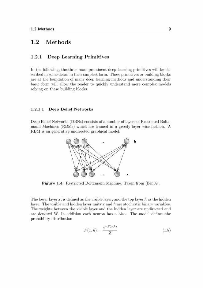
Deep Belief Networks (DBNs) consists of a number of layers of Restricted Boltz-mann Machines (RBMs) which are trained in a greedy layer wise fashion. ARBM is an generative undirected graphical model.
Figure 1.4: Restricted Boltzmann Machine. Taken from [Ben09].
The lower layer x, is defined as the visible layer, and the top layer h as the hiddenlayer. The visible and hidden layer units x and h are stochastic binary variables.The weights between the visible layer and the hidden layer are undirected andare denoted W. In addition each neuron has a bias. The model defines theprobability distribution
P (x, h) =e−E(x,h)
Z(1.8)

1.2 Methods 10
With the energy function, E(x, h) and the partition function Z being defined as
E(x, h) = −b′x− c′h− h′Wx (1.9)
Z(x, h) =∑x,h
e−E(x,h) (1.10)
Where b and c are the biases of the visible layer and the hidden layer respec-tively. The sum over x, h represents all possible states of the model.The conditional probability of one layer, given the other is
P (h|x) =exp(b′x+ c′h+ h′Wx)∑h exp(b′x+ c′h+ h′Wx)
(1.11)
P (h|x) =
∏i exp(cihi + hiWix)∏
i
∑h exp(cihi + hiWix)
(1.12)
P (h|x) =∏i
exp(hi(ci +Wix))∑h exp(hi(ci +Wix))
(1.13)
P (h|x) =∏i
P (hi|x) (1.14)
Notice that if one layer is given, the distribution of the other layer is factorial.Since the neurons are binary the probability of a single neuron being on is givenby
P (hi = 1|x) =exp(ci +Wix)
1 + exp(ci +Wix)(1.15)
P (hi = 1|x) = sigm(ci +Wix) (1.16)
Similarly the conditional probability for the visible layer can be found
P (xi = 1|h) = sigm(bi +Wih) (1.17)
In other words, it is a probabilistic version of the normal sigmoid neuron ac-tivation function. To train the model, the idea is to make the model generatedata like the training data. Mathematically speaking we wish to maximize thelog probability of the training data or minimize the negative log probability ofthe training data.The gradient of the negative log probability of the visible layer with respect to

1.2 Methods 11
the model parameters θ is
∂
∂θ(− logP (x)) =
∂
∂θ
(− log
∑h
P (x, h)
)
=∂
∂θ
(− log
∑h
exp(−E(x, h))
Z
)
= − Z∑h exp(−E(x, h))
(∑h
1
Z
∂ exp(−E(x, h))
∂θ−∑h
exp(−E(x, h))
Z2
∂Z
∂θ
)
=∑h
(exp(−E(x, h))∑h exp(−E(x, h))
∂E(x, h)
∂θ
)+
1
Z
∂Z
∂θ
=∑h
P (h|x)∂E(x, h)
∂θ− 1
Z
∑x,h
exp(−E(x, h))∂E(x, h)
∂θ
=∑h
P (h|x)∂E(x, h)
∂θ−∑x,h
P (x, h)∂E(x, h)
∂θ
= µ1
[∂E(x, h)
∂θ
∣∣∣∣x]− µ1
[∂E(x, h)
∂θ
]∂
∂W(− logP (x)) = µ1 [−h′x|x]− µ1 [−h′x]
∂
∂b(− logP (x)) = µ1 [−x|x]− µ1 [−x]
∂
∂c(− logP (x)) = µ1 [−h|x]− µ1 [−h]
where µ1 is a function returning the first moment or expected value. The firstcontribution is dubbed the positive phase, and it lowers the energy of the trainingdata, the second contribution is dubbed the negative phase and it raises theenergy of all other visible states the model is likely to generate.The positive phase is easy to compute as the hidden layer is factorial given thevisible layer. The negative phase on the other hand is not trivial to compute asit involves summing all possible states of the model.Instead of computing the exact negative phase, we will sample from the model.Getting samples from the model is easy; given some state of the visible layer,update the hidden layer, given that state, update the visible layer, and so on,

1.2 Methods 12
i.e.
h(0) = P (h|x(0))x(1) = P (x|h(0))h(1) = P (h|x(1))
...
x(n) = P (x|h(n−1))
The superscripts denote the order in which each calculation is made, not thespecific neuron of the layer. At each iteration the entire layer is updated. Toget unbiased samples, we should initialize the model at some arbitrary state,and sample n times, n being a large number. To make this efficient, we’ll dosomething slightly different. We’ll initialize the model at a training sample,iterate one step, and use this as our negative sample. This is the contrastivedivergence algorithm as introduced by Hinton [HOT06] with one step (CD-1).The logic is that, as the model distribution approaches the training data dis-tribution, initializing the model to a training sample approximates letting themodel converge.Finally, for computational efficiency, we will use stochastic gradient descent in-stead of the batch update rule derived. Alternatively one can use mini-batches.The final RBM learning algorithm can be seen below. α is a learning rate andrand() produces random uniform numbers between 0 and 1.
Algorithm 1 Contrastive Divergence 1
for all training samples as t dox(0) ← th(0) ← sigm(x(0)W + c) > rand()x(1) ← sigm(h(0)WT + b) > rand()h(1) ← sigm(x(1)W + c) > rand()W ←W + α(x(0)h(0) − x(1)h(1))b← b+ α(x(0) − x(1))c← c+ α(h(0) − h(1))
end for
Being able to train RBMs we now turn to putting them together to form deepbelief networks. The idea is to train the first RBM as described above, thentrain another RBM using the first RBM’s hidden layer as the second RBMsvisible layer.

1.2 Methods 13
Figure 1.5: Deep Belief Network. Taken from [Ben09].
To train the second RBM, a training sample is clamped to x, transformed toh1 by the first RBM and then contrastive divergence is used to train the secondRBM. As such training the second RBM is exactly equal to training the firstRBM, except that the training data is mapped through the first RBM beforebeing used as training samples. The intuition is that if the RBM is a generalmethod for extracting a meaningful representation of data, then it should beindifferent to what data it is applied to. Popularly speaking, the RBM doesn’tknow whether the visible layer is pixels, or the output of another RBM, orsomething different altogether. With this intuition it becomes interesting toadd a second RBM, to see if it can extract a higher level representation ofthe data. Hinton et al have shown, that adding a second RBM decreases avariational band on the log likelihood of the training data [HOT06].Having trained N layers in this unsupervised greedy manner, Hinton et al, addsa last RBM and adds a number of softmax neurons to its visible layer. Thesoftmax neurons are then clamped to the labels of the training data, such thatthey are 0 for all except the neuron corresponding to the label of the trainingsample, which is set to 1. In this way, the last RBM learns a joint model of thetransformed data, and the labels.

1.2 Methods 14
Figure 1.6: Deep Belief Network with softmax label layer. Taken from[HOT06].
To use the DBN for classification, a sample is clamped to the lowest level visiblelayer, transformed upwards through the DBN until it reaches the last RBMshidden layer. In these upward passes the probabilities of hidden units beingon are used directly instead of sampling, to reduce noise. At the top RBM, afew iterations of gibbs sampling is performed after which the label is read out.Alternatively the exact ’free energy’ of each label can be computed and the onewith the lowest free energy is chosen [HOT06]. To fine-tune the entire modelfor classification Hinton et al uses an ’up-down’ algorithm [HOT06].Simpler ways to use the DBN for classification are to simply use the top levelRBM hidden layer activation in any standard classifier or to add a last labellayer, and train the whole model as a feedforward-backpropagate neural network.If one of the latter methods are used, then there is no need to train the lastRBM as a joint model of data and labels.
1.2.1.2 Stacked Autoencoders
Stacked Autoencoders are, as the name suggests, autoencoders stacked on topof each other, and trained in a layerwise greedy fashion.An autoencoder or auto-associator is a discriminative graphical model that at-tempts to reconstruct its input signals.

1.2 Methods 15
Figure 1.7: Autoencoder. Taken from [Ben09].
There exists a plethora of proposed autoencoder architectures; with/withouttied weights, with various activation functions, with deterministic/stochasticvariables, etc. This section will use the autoencoder desribed in [BLP+07] as abasic example implementation which have been used successfully as a buildingblock for deep architectures.Autoencoders take a vector input x, encodes it to a hidden layer h, and decodesit to a reconstruction z.
h(x) = sigm(W1x+ b1) (1.18)
z(x) = sigm(W2h(x) + b2) (1.19)
To train the model, the idea is to minimize the average difference between theinput x and the reconstruction z with respect to the parameters, here denotedθ.
θ = argminθ
1
N
N∑i=1
L(x(i), z(x(i))) (1.20)
Where N is the number of training samples and L is a function that mea-sures the difference between x and z, such as the traditional squared errorL(x, z) = ||x − z||2 or if x and z are bit vectors or bit probabilities, the cross-entropy L(x, z) = xT log(z) + (1− x)T log(1− z)Updating the parameters efficiently is achieved with stochastic gradient descentwhich can be efficiently implementing using the backpropagation algorithm.
There is a serious problem with autoencoders, in that if the hidden layer is thesame size or greater than the input and reconstruction layers, then the algo-rithm could simply learn the identity function. If the hidden layer is smallerthan the input layer, or if other restrictions are put on its representation, e.g.sparseness, then this is not an issue.
Having trained the bottom layer autoencoder on data, a second layer autoen-coder can be trained on the activities of the first autoencoders hidden layer when

1.2 Methods 16
exposed to data. In other words the second autoencoder is trained on h(1)(x)and the third autoencoder would be trained on h(2)(h(1)(x)), etc, where thesuperscripts denote the layer of the autoencoder. In this way multiple autoen-coders can be stacked on top of each other and trained in a layer-wise greedyfashion, which has been shown to lead to good results [VLBM08].
To use the model for discrimination, the outputs of the last layer can be usedin any standard classifier. Alternatively a last supervised layer can be added,and the whole model trained as a feedforward-backpropagate neural network.
1.2.1.3 Convolutional Neural Nets
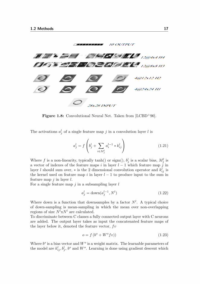
Convolutional Neural Networks (CNNs) are feedforward, backpropagate neuralnetworks with a special architecture inspired from the visual system. Hubel andWiesel’s early work on cat and monkey visual cortex showed that the visualcortex is composed of cells with high specificity to patterns within a localizedarea, called their receptive fields [HW68]. These so called simple cells are tiledas to cover the entire visual field and higher level cells recieve input from thesesimple cells, thus having greater receptive fields and showing greater invarianceto translation. To mimick these properties Yan Lecun introduced the Convolu-tional Neural Network [LCBD+90], which still hold state-of-the art performanceon numerous machine vision tasks [CMS12] and acts as inspiration to recent re-seach [SWB+07], [LGRN09].
CNNs work on the 2 dimensional data, so called maps, directly, unlike normalneural networks which would concatenate these into vectors. CNNs consists ofalternating layers of convolution layers and sub-sampling/pooling layers. Theconvolution layers compose feature maps by convolving kernels over featuremaps in layers below them. The subsampling layers simply downsample thefeature maps by a constant factor.
1.2 Methods 17
Figure 1.8: Convolutional Neural Net. Taken from [LCBD+90].
The activations alj of a single feature map j in a convolution layer l is
alj = f
blj +∑i∈M l
j
al−1i ∗ klij
(1.21)
Where f is a non-linearity, typically tanh() or sigm(), blj is a scalar bias, M lj is
a vector of indexes of the feature maps i in layer l − 1 which feature map j inlayer l should sum over, ∗ is the 2 dimensional convolution operator and klij isthe kernel used on feature map i in layer l − 1 to produce input to the sum infeature map j in layer l.For a single feature map j in a subsampling layer l
alj = down(al−1j , N l) (1.22)
Where down is a function that downsamples by a factor N l. A typical choiceof down-sampling is mean-sampling in which the mean over non-overlappingregions of size N lxN l are calculated.To discriminate between C classes a fully connected output layer with C neuronsare added. The output layer takes as input the concatenated feature maps ofthe layer below it, denoted the feature vector, fv
o = f (bo +W ofv)) (1.23)
Where bo is a bias vector andW o is a weight matrix. The learnable parameters ofthe model are klij , b
lj , b
o and W o. Learning is done using gradient descent which

1.2 Methods 18
can be implemented efficiently using a convolutional implementation of the back-propagation algorithm as shown in [Bou06]. It should be clear that becausekernels are applied over entire input maps, there are many more connections inthe model than weights, i.e. the weights are shared. This makes learning deepmodels easier, as compared to normal feedforward-backprop neural nets, as thereare fewer parameters, and the error gradients goes to zero slower because eachweight has greater influence on the final output.
1.2.1.4 Sparsity
Sparse coding is the paradigm that data should be represented by a small subsetof available basis functions at any time, and is based on the observation thatthe brain seems to represent information with a small number of neurons atany given time [OF04]. Sparsity was originally investigated in the context ofefficient coding and compressed sensing and was shown to lead to gabor-likefilters [OF97]. They are not directly related to deep architectures, but theirinteresting encoding properties have lead to them being used in deep learningalgorithms in various ways.
The most direct use of sparse coding can be seen as formulating a new basisfor a dataset which is composed of a feature vector and a set of basis functions,while restricting the feature vector to be sparse.
x = Aa (1.24)
Where x ∈ <n is the data, A ∈ <nxm is the m basis functions and a ∈ <m isthe ”sparse” vector describing which sum of basis functions represent the data.a is sparse in the sense that it is mostly zero, i.e. few basis functions are usedat all times to represent any data. In images this is in contrast to the normalnon-sparse representation used, which is pixel intensities. This corresponds toA = Inxn, i.e A being a square identity matrix, and a being the normal vectorrepresentation of image intensities.
In a deep learning setting, a non-sparsity penalty, i.e. measuring how much theneurons are active on average, can be added to the loss function. If the neuronsare binomial, sparse coding could correspond to restricting the mean numberof activate hidden neurons to some fraction. If the neurons are continuousvalued, this could correspond to restricting the mean of all hidden units tosome constant. Sparse variants of RBMs and autoencoders have been proposed

1.2 Methods 19
[GLS+09, PCL06]. A sparse autoencoder has a second contribution to its lossfunction, the non-sparsity measure:
L(x, z) = ||x− z||2 + β||h− ρ|| (1.25)
Where β is a constant describing how much being non-sparse should be penalizedand ρ is a constant close to the lower boundary of the output of the hiddenneurons h. In the case of sigmoidal hidden neurons, this could be ρ = 0.1. Inthe case of tanh hidden neurons this could be ρ = −0.9
1.2.2 Key Points
1.2.2.1 Training Deep Architectures
A key element to Deep Learning is the ability to learn from unlabelled data asit is available in vast quantities, e.g. video or images of natural scenes, sound,etc. This is also referred to as unsupervised training. This is in contrast to su-pervised training which is training on labelled data, of which there is relativelylittle, and which is much harder to generate. To get unlabelled video data onemight simply go onto youtube.com and download a million hours of video, butto get 1 hour of labelled video data one would need to painstakingly segmenteach frame into the objects of interest. Further, being able to learn on the unla-belled data gives one a high-dimensional learning signal, whereas most labelleddata is relatively low-dimensional, e.g. a label specifying cat or dog is two bitsof information whereas a 100x100 pixels image of a cat or dog in true color is24*3*100*100 = 720.000 bits.
Machine Learning models are rarely built to achieve good performance on unla-belled data though; usually some kind of classification or regression is required.The idea then is to train the model on the unlabelled data first, called pre-training, to achieve good features or representations of the data. Once this hasbeen achieved the parameters learned are used to initiate a model, which istrained in a supervised fashion to fine-tunes the parameters to the task at hand.
Deep belief nets and stacked auto encoders both use the same method for pre-training: training each layer unsupervised on the activations of the layer below,one after another. Convolutional neural nets stand out in this aspect, as theydo not use pre-training. Since CNNs have substantially less parameters, andtranslation invariance is built into the model, there seems to be less need for pre-training. Pre-training convolutional neural nets in a layer-wise fashion similar
1.3 Results 20
to DBNs and SAEs have been shown to be slightly superior to randomly initial-ized networks though [MMCS11]. Generally the paradigm of greedy layer-wisepre-training followed by global supervised training to fine-tune the parametersseems to give good results.
The theory as to why this works well is that the unsupervised pre-training movesthe parameters to a region in parameter space that is closer to a global optimumor at least a region which represents the data more naturally. Numerical studieshave shown that pre-trained and randomly initialized networks do indeed endup in very different regions of parameter space after having been trained on asupervised task [EBC+10]. Also, the global supervised learning rarely changesthe pre-trained parameters much, what happens instead is a fine-tuning to im-prove on the supervised task [EBC+10].
After pre-training, instead of training the model globally on the supervised taskone can instead use any standard supervised learning model on the output fea-tures of the pre-trained model, e.g. pre-training a Deep Belief Network, andthen using the activity of the top output neurons as input in a SVM, logisticregression, etc.
Alternatively one can train the model in a supervised and unsupervised set-ting at the same time, alternating between the two learning modes or having acomposite learning rule. This is known as semi-supervised learning.
1.3 Results
The three primitives, DBNs, SAEs and CNNs were implemented and evaluatedon the MNIST dataset to illustrate state of the art in Deep Learning. The er-ror rates achieved for the DBN, SAE and CNN were 1.67%, 1.71% and 1.22%,respectively. The error rates compared to state-of-the art with comparable net-work architectures for the DBN and SDAEs are slightly worse whereas the CNNerror rate is slightly better.

1.3 Results 21
DBN (1000-1000-1000) SAE (1000-1000-1000) CNN (c6-d2-c72-d2)1.67 % 1.71 % 1.22 %
Table 1.1: Error rates of three deep learning primitives. The DBN and SAEboth had 3 hidden layers each with 1000 neurons. The CNN had thefollowing layers: 6 feature maps using 5x5 kernels, 2x2 mean-pooldownsampling, 72 feature maps using 5x5 kernels, 2x2 downsam-pling and a fully connected output layer.
The MNIST dataset [LBBH98] contains 70.000 labelled images of handwrittendigits. The images are 28 by 28 pixels and gray scale. The dataset is dividedinto a training set of 60.000 images and a test set of 10.000 images. The datasethas been widely used as a benchmark of machine learning algorithms. In thefollowing details of the implementations of the three models on MNIST is de-scribed and results on MNIST are shown.
Figure 1.9: A random selection of MNIST training images.
Except otherwise noted all experiments used the sigmoid non-linearity for allneurons, initialized the biases to zero and drew weights from a uniform randomdistribution with upper and lower bounds ±
√6/(fanin + fanout) as recom-
mended in [LBOM98]. All experiments were run on a machine with a 2.66 GHzIntel Xeon Processor and 24 GB of memory.

1.3 Results 22
1.3.1 Deep Belief Network
A three layer DBN were constructed. The net consisted of three RBMs each with1000 hidden neurons, and each RBM was trained in a layer-wise greedy mannerwith contrastive divergence. All weights and biases were initialized to be zero.Each RBM was trained on the full 60.000 images training set, using mini-batchesof size 10, with a fixed learning rate of 0.01 for 100 epochs. One epoch is one fullsweep of the data. The mini-batches were randomly selected each epoch. Havingtrained the first RBM the entire training dataset was transformed through thefirst RBM resulting in a new 60.000 x 1000 dataset which the second RBM wastrained on and similarly so for the third RBM. Having pre-trained each RBMthe weights and biases were used to initialize a feed-forward neural net with4 layers of sizes 1000-1000-1000-10, the last 10 neurons being the output labelunits. The FFNN was trained using mini-batches of size 10 for 50 epochs usinga fixed learning rate of 0.1 and a small L2 weight-decay of 0.00001 using back-propagation. To evaluate the performance the test set was feed-forwarded andthe maximum output unit was chosen as the label for each sample resulting inan error rate of 1.67% or 167 errors out of the 10.000 test samples. The coderan for 28 hours.
Figure 1.10: Weights of a random subset of the 1000 neurons of the first RBM.Each image is contrast normalized individually to be betweenminus one and one.
The first RBM has to a large degree learned stroke and blob detectors as canbe seen from the weights. Less meaningful detectors are also present either re-flecting the higly over-parametrized nature of the RBM or a lack of learning.Given the good performance it is probable that the dataset could be sufficiently

1.3 Results 23
represented by the other neurons.
Figure 1.11: The 167 errors using a 3 layer DBN with 1000, 1000 and 1000neurons respectively.
While some of the images are genuinely difficult to label, a number of themseems easy. Many of the sevens in particular seem fairly easy. The added intra-class variation due to continental sevens and regular sevens might explain thisto a degree.
Hinton showed an error rate of 1.25% in his paper introducing the DBN andcontrastive divergence [HOT06]. This impressive performance was achieve witha 3 layer DBN with 500, 500 and 2000 hidden units respectively, training acombined model of the representation and the labels in the last layer togetherand using extensive cross validation to tune the hyper parameters. AdditionallyHinton used a novel up-down algorithm to tune the weights on the classificationtask, running a total of 359 epochs resulting in a learning time of about a week.It has been shown [VLL+10] that pre training a DBN, using its weights toinitialize a deep FFNN and training that on a supervised task with stochasticbackpropagation can lead to the same error rates as those reported by Hinton.As such it seems that it is not the training regime used resulting in the highererror rate but rather a need for further tuning of the hyper parameters.

1.3 Results 24
1.3.2 Stacked Denoising Autoencoder
A three layer stacked denoising autoencoder (SDAE) with architecture identicalto the DBN was created. The denoising autoencoder works just like the normalautoencoder except that the input is corrupted in some way, and the autoencoderis trained to reconstruct the un-corrupted input [VLBM08]. The idea is thatthe autoencoder cannot simply copy pixels and will have to learn corruptioninvariant features to reconstruct well. The corruption process used was settinga randomly selected fraction of the pixel in the input image to zero. The SDAEconsisted of three denoising autoencoder (DAE) stacked on top of each othereach with 1000 hidden neurons, and each trained in a greedy-layer wise fashion.Each DAE was pre-trained with a fixed learning rate of 0.01 and a batchsizeof 10 for 30 epochs and with a corruption fraction of 0.25 i.e. a quarter ofthe pixels set to zero in the input images. The noise level was chosen basedon conclusions from [VLL+10]. Having trained the first DAE the training setwas feed-forwarded through the DAE and the second DAE was trained on thehidden neuron states of the first DAE, and similarly for the third DAE. After pre-training in this manner the upwards weights and biases were used to initializea FFNN with 10 output neurons in the same manner as for the DBN. TheFFNN was trained with a fixed learning rate of 0.1, with a batchsize of 10 for30 epochs. The performance was measured as for the DBN resulting in an errorrate of 1.71% or 171 errors. The code ran for 41 hours.
Figure 1.12: Left: Weights of a random subset of the 1000 neurons of a DAEwith a corruption level of 0.25. Right: DAE trained in a similarmanner with a corruption level of 0.5. The second DAE hadworse discriminative performance. Its weights are shown hereonly to show that DAEs can find good representations. Eachimage is contrast normalized individually to be between minusone and one.

1.3 Results 25
The DAE seems to find mostly seemingly non-sensical and blob detectors. Forreference the weights of another DAE trained in a similar manner with a cor-ruption level of 0.5 is provided. The latter finds stroke detectors and seem lessnoisy. The latter DAE had worse discriminative performance (not shown).
Figure 1.13: The 171 errors using a 3 layer SDAE with 1000,1000 and 1000neurons respectively.
In [VLBM08] Pascal Vincent introduces the denoising autoencoder and reportssuperior performance on a number of MNIST like tasks. The basic MNIST testscore is not reported though until his 2010 paper [VLL+10] in which Vincentreports an error rate of 1.28% on MNIST with a three layer SDAE using 25%corruption and extensive cross validation to tune the hyperparameters. The 1.71% error rate here is on the same order of magnitude but compares unfavourablyto the 1.28 %. It is evident that further tuning of the hyper parameters wouldhave been beneficial.
1.3.3 Convolutional Neural Network
A Convolutional Neural Network was created following the architecture in [LCBD+90]in which Yann LeCun introduces the CNN. The first layer has 6 feature mapsconnected to the single input layer through 6 5x5 kernels. The second layer isa a 2x2 mean-pooling layer. The third layer has 12 feature maps which are allconnected to all 6 mean-pooling layers below through 72 5x5 kernels. This full

1.3 Results 26
connection between layer 2 and 3 is in contrast to the architecture proposedby LeCun, which used a hand-chosen set of connections. The fourth layer is a2x2 mean-pooling layer. When training, the feature maps of this fourth layeris concatenated into a feature vector which feeds into the fifth and final layerwhich consists of 10 output neurons corresponding to the 10 class labels.The CNN was trained with stochastic gradient descent on the full MNIST train-ing set. A batch size of 50 and a fixed learning rate of 1 was used for 100 epochsresulting in a test score of 1.22% or 122 misclassifications. The code ran for 7hours.
Figure 1.14: Left: The 6 kernels of the first layer. Right: The 72 kernels ofthe third layer. All kernels are contrast normalized individuallyto be between minus and plus one.
The CNNs 6 first layer kernels seems to be 4 curvy stroke detectors and two lesswell defined detectors. The 72 layer three kernels cannot be directly analysedwith respect to what detectors they are as they operate on already transformedinput. There does seem to be some structure in them though reflecting that thefeature maps in layer 2 are still resembling digits.

1.3 Results 27
Figure 1.15: The 122 errors with the CNN.
The MNIST dataset did not exist at the time LeCun introduced the CNN.However in his 1998 paper [LBBH98] he reports a 1.7 % error for a networkof this architecture, which he names LeNet1. Lecun subsamples the images to16x16 pixels and uses a second order backprop method to achieve the 1.7%.The 1.22 % error rate compares favourably with this as there were no pre-processing and simple first-order backprop with a fixed learning rate was used.It should be noted that LeCun reports an error rate of 0.95% with LeNet-5, amore advanced net in the same paper. As no cross-validation was used to findthe hyper-parameters the performance could probably be increased with furthertuning of the hyper-parameters. It is remarkable that such a simple architectureas LeNet-1 is able to achieve such good performance.

Chapter 2
A prediction learningframework
2.1 Introduction
2.1.1 The case for a prediction based learning framework
As described autoencoders works by encoding a visible input to a hidden rep-resentation and decoding it back to a reconstruction of the input. The learningis then done by minimizing the difference between the reconstruction and theinput. As described these models can just learn the identity and to achievefeature detectors akin to those expected, i.e. edge detectors or gabor-like filters,most authors see the need to make the reconstruction more challenging. Manypapers use sparsity to this end, and describe that without this, the model didnot find good feature detectors [LGRN09, GLS+09], others, such as the denois-ing autoencoder applies noise to the input image.
When reconstructing input, there are, obviously, no changes from the inputto the output. In other words there are no transformations. It might seemcurious then that we hope to find representations that are invariant to transfor-mations, such as small translations, noise, illumination, etc. The logic is that if

2.1 Introduction 29
we present the model with enough data where these transformations take placebetween samples, i.e. one sample may be a shifted or noisy version of anothersample, then the model will learn representations invariant to the presentedtransformations. This makes sense as an invariant feature detector will on aver-age create better reconstructions. If the model is over-saturated however, thereis less need for sharing features amongst samples and heuristics are needed toachieve invariant feature detectors, as described above.
A more direct approach to achieve invariance might be to train the model oninvariant output and transformed input; the transformations applied to the in-put being exactly the transformations we wish to achieve invariance to. Featuredetectors would be forced to be invariant to something in order to reconstructcorrectly and the sum of feature detectors should be invariant to all appliedtransformations.
The denoising autoencoder can be seen in this light as it adds noise to the inputand reconstructs the clean input. The transformation applied here is noise andthe invariance we achieve is invariance to noise. We could explore this furtherby rotating, translating, elastically deforming, etc. the input data and recon-structing the clean output. But adding the transformations we wish to achieveinvariance to explicitly seems like a poor solution. Further, our human intuitionabout the desired invariances will not work as well when we add additional layersand need to describe the needed invariances of say, a rotation detector. Ideallywe would like a model that could be trained fully unsupervised, and achieveinvariances not limited to the extent of its authors understanding of the data.
I hypothesize that the transformations taking place over time are exactly thetransformations we wish to achieve invariance to and as such, prediction wouldbe a far better candidate for learning than reconstruction. In the case of video,the frame to frame differences include translation, rotation, noise, illuminationchanges, etc. In short all the transformations that we wish to achieve invari-ance to. A model predicting video frames would take some number of previousframes and attempt to predict the next frame. Training a model like this is aninstance of the previously described more direct approach to learning in whicheach learning sample contains transformations.
Furthermore, prediction is a much harder task than simple reconstruction and itis hypothesized that as such the model would be much less prone to over fittingand see less need for heuristics such as sparsity, weight decay, etc.

2.1 Introduction 30
From a biological standpoint prediction as a candidate for learning makes goodsense. Being able to predict the environment and the consequences of ones ac-tions is arguably what give intelligent life an advantage. Jeff Hawkins makesthis argument at length in [HB04] and Karl Friston suggests minimization offree energy, or prediction error, as the foundation for a unified brain theory[Fri03]. One very appealing feature of prediction as a learning framework isthat the learning signal, the prediction error, is unsupervised and readily avail-able. There is no need for an external source of learning or complex setups fordefining the learning signal. Instead predictions are made at all time at theneural level, and prediction error drives the learning. One of Jeff Hawkins waysto illustrate that the brain is making predictions at all times is to point out thatyou know what the last word in this sentence is before it ends.
Recent understandings [SMA00] of the mechanisms behind long term potenta-tion and de-potentation in the neural connections can be seen in the light of theprediction learning framework as well. Specifically the theory of spike-timingdependent plasticity (STDP) describes that if the pre-synaptic neuron deliversinput to the post-synaptic neuron shortly before the post-synaptic neuron fires,their connection is strengthened and if it delivers it after the post-synaptic neu-ron have fired, their connection is weakened. In short, if a pre-synaptic neuroncan predict the firing of the post-synaptic neuron their connection is strength-ened and if not, their connection is weakened. Experiments have shown thatimplementing a STDP learning rule in a network of artificial neurons can leadto the network predicting input sequences [RS01].
Prediction as a learning framework fits well with the array of evidence pointingto a vast amount of top-down connections in the brain[EGHP98], which areeven expected to exceed the number of bottom-up connections [SB95]. It hasbeen shown that these top-down connections modulate the bottom-up input atmultiple stages in the visual pathway. [AB03, SKS+05]. Also, there is an asym-metry in the bottom-up and the top-down connections effect. ”In particular,while bottom-up projections are driving inputs (i.e., they always elicit a responsefrom target regions), top-down inputs are more often modulatory (i.e., they canexert subtler influence on the response properties in target areas), although theycan also be driving” [KGB07].
2.1.2 Temporal Coherence
Temporal coherence is tightly linked to prediction and as such will briefly be re-viewed here. Temporal Coherence is the observation that, generally, the objects

2.1 Introduction 31
giving rise to the sensory inputs are changing slowly over time. The objects inmention here could be trees, or the sun or concepts such as time of day, whichare combined in a highly non-linear way to create the sensory inputs we per-ceive. Whereas the objects are slowly and smoothly changing, i.e. a personwalking from one end of the room to the other, the sensory signals might berapidly and seemingly randomly changing, i.e. the pixels seen might alternatequickly between black and white as the persons clothing folds and shadows arecast.
The principle of Temporal Coherence been attempted to be used for learningin the past [F91, Sto96] and more recently have been attempted as a learningprinciple for deep learning approaches. Two such approaches will be outlinedshortly here to illustrate how the idea can be applied.
One application of temporal coherence is to force deep representation to be tem-porally coherent in some standard deep learning method as seen in [MMC+09].The paper uses a convolutional neural net on a supervised learning task. It in-troduces an extra unsupervised learning signal though, such that their algorithmbecomes:
• input a labelled image, and take a gradient step to minimize classificationerror.
• input two consecutive image from unlabelled video and take a gradientstep to maximize the temporal coherence in layer N.
• input two non-consecutive images from unlabelled video and take a gra-dient step to minimize the temporal coherence in layer N.
This learns the model to classify labelled images while it forces the represen-tations in layer N to be temporally coherent. The paper sets layer N as theirnext-deepest layer, the logic being that this should be the most high-level rep-resentation of the image and thus should be varying the slowest.
Another more direct application of temporal coherence is seen in Slow FeatureAnalysis (SFA). SFA focuses on extracting slowly varying time signals from timesequences. In short SFA seeks to transform a N dimensional time signal to anMN dimensional feature space in which each features temporal variance is min-imized under the constraint that the features cannot be trivial i.e. being zeroor having zero variance and that each feature should be different (uncorrelated)

2.1 Introduction 32
[BW05]. How to find the MN dimensional feature spaces, e.g. learn in themodel is explained in [WS02] and is beyond the scope of this thesis. It shouldbe noted that SFA can be applied recursively, e.g. in a layer wise fashion wherethe output of one SFA is the input to the next.
SFA has been applied to natural images undergoing various transformations overtime such as rotation, translation, etc, and lead to a rich repertoire of complexcell like filters [BW05] as well as successfully applied to artificial data [WS02].
2.1.3 Evaluating Performance
When designing deep learning modules, it is difficult to evaluate their perfor-mance quantitatively. Ultimately such modules are to be used in a deep archi-tecture, on some classification task, but until the module itself have been shownto find good representations of the data there is little point in building a biggermodel comprising many such modules to evaluate it using a classification task.As such the majority of the evaluation of the following proposed models will bequalitative, looking at what representations the modules find. As the proposedmodels all work on natural video the receptive fields found will be compared tothe receptive fields of the primate visual cortex.
Figure 2.1: Estimated Spatio-Temporal receptive field of Macaque monkey.Top: Example of a receptive field resembling a blob-detector. Bot-tom: Example of an oriented spatio-temporal receptive field. Timein miliseconds is superimposed (upper right corner, tilted) on eachimage. Taken from [Rin02].

2.2 The Predictive Encoder 33
Figure 2.2: Estimated receptive field of Macaque monkey at their optimaltime-delay. Several receptive fields resembling gabor filters at var-ious orientations are visible. Taken from [Rin02].
Figure 2.1 and 2.2 shows the spatio-temporal and spatial receptive fields found inMacaque monkeys[Rin02] consistent with previous findings [HW68]. For modelstrained on video of natural scenes these are the kind of receptive fields themodules are supposed to find, i.e. oriented gabor filters.
2.2 The Predictive Encoder
The following section introduces the Predictive Encoder (PE) as a candidate fora prediction based deep learning model.
2.2.1 Method
The Predictive Encoder (PE) is an autoencoder that instead of reconstructingan input, attempts to predict future input, given n previous inputs. It encodesthe concatenated previous inputs into a hidden representation and decodes thehidden representation to a prediction of the future inputs.
Figure 2.3: Predictive Encoder with n = 2 previous input. Modified from[Ben09].
The governing equations of the PE are very similar to that of a simple autoen-coder.

2.2 The Predictive Encoder 34
h(x) = f(W1xt−1,t−2,...,t−n + b) (2.1)
z(x) = f(W2h+ c) (2.2)
L(x) =1
2||z − xt||2 (2.3)
Where h is a vector of hidden representations, f is a non-linearity, typicallysigm or tanh, W1 is the encoding weight matrix, xt−1,t−2,...,t−n is a concate-nated vector of the n previous inputs, b is a vector of additive biases for thehidden representations, z is a vector representing the prediction given by thePE, W2 is the decoding weight matrix, c is a vector of additive biases, L is thesum square loss function and xt is the input at time t, which the PE is trying topredict. Learning is done by updating the parameters W1,W2, b, c with stochas-tic gradient descent.
The PE can be trained layer-wise and stacked on top of each other, each trainedon the hidden states of the PE below creating the Stacked Predictive Encoder(SPE) comparable to stacked auto-encoders or DBNs.
2.2.1.1 Relation to other models
Figure 2.4: CRBM with n = 2 previous input. Taken from [THR11].
The Predictive Encoder bears close resemblance to a Conditional RestrictedBoltzmann Machine [THR11] (CRBM). The main differences are that the CRBM
2.2 The Predictive Encoder 35
has directed connections between the previous inputs and the input to be pre-dicted, undirected connections between the hidden layer and the input to bepredicted, has stochastic neurons and uses contrastive divergence instead ofbackprop for learning. There is no reason the Predictive Encoder cannot haveconnections from previous inputs directly to the input to be predicted as theCRBM does. In the CRBM these connections primarily serve to model simplespatio-temporal pixel to pixel correlations, in effect a kind of whitening [THR11]which frees up the hidden layer to focus on higher order dependencies. If thedata has been pre-whitened these might be less useful. CRBMs have been usedin modelling motion capture data [THR11] and phone recognition [MH10] withgood results for both. The predictive encoder can be seen as a simpler deter-ministic variant of the CRBM, which is simpler to train.
Two related and highly influential models of cortical functions are PredictiveCoding (PC) [SLD82, RB99] and Biased Competition (BC) [DD95, Bun90].Predictive coding is a model of cortical function hypothesizing that top downinformation predicts bottom up information, and inhibits all bottom up in-formation consistent with the prediction. In this way only the error signal ispropagated upwards, which allows for efficient coding of redundant/predictablestructures. Biased Competition is the seemingly opposite theory that top-downinformation enhances bottom-up information consistent with the top-down in-formation, serving to solve a competition for activity, i.e. solve which neuralrepresentation gets to represent the input. The two models have been shownto be equal under certain conditions [Spr08]. PC has been shown to replicateend-stopping and other extra-classical receptive field effects [RB99] and two PCmodels have been shown to lead to gabor like receptive fields when trained onnatural images [RB99, Spr12]. The proposed predictive encoder differs fromthese models in that while they both mention an extension to temporal data,they concentrate on the spatial predictions whereas the predictive encoder isonly defined for temporal data and inherently learns on spatio-temporal pat-terns.
The predictive encoder can be seen as a denoising autoencoder which appliesa corruption process learned naturally from the data. Vincent ends his thor-ough paper on denoising autoencoders discussing the benefits of this. ”If moreinvolved corruption processes than those explored here prove beneficial, it wouldbe most useful if they could be parametrized and learnt directly from the data,rather than having to be hand-engineered based on prior-knowledge.” [VLL+10].As mentioned it is hypothesized that the variations occurring over time are ex-actly equal to the noise we wish to achieve invariance to and as such shouldprove beneficial. The PE and the DAE differ in that the former is defined fortemporal data whereas the latter is defined for non-temporal data. The PE re-
2.2 The Predictive Encoder 36
duces to a denoising autoencoder if the only noise occurring over time is randomand independent, such as a noisy neuron looking at the same input over severaltime-steps.
2.2.2 Dataset
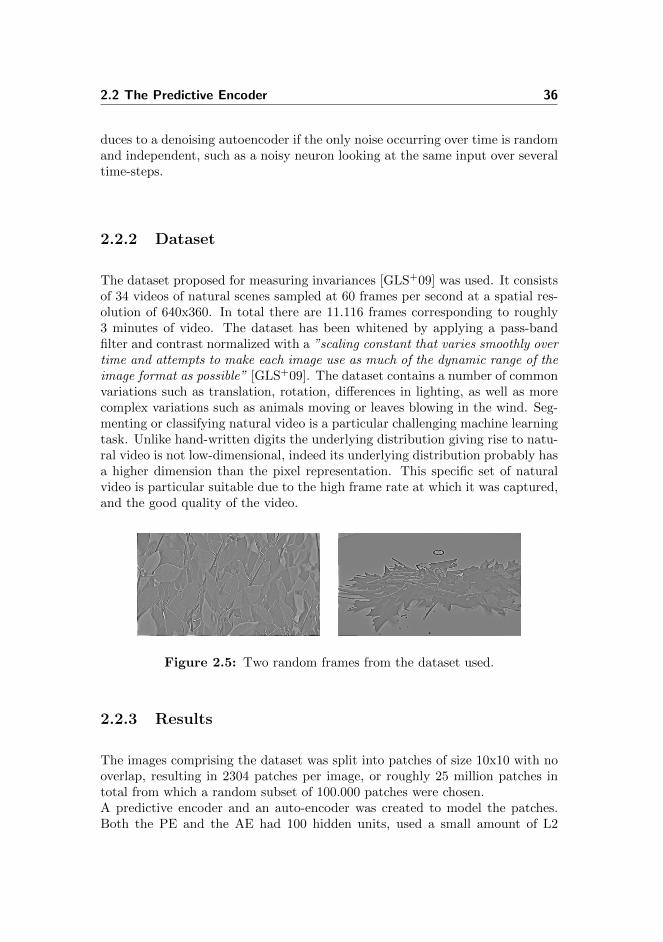
The dataset proposed for measuring invariances [GLS+09] was used. It consistsof 34 videos of natural scenes sampled at 60 frames per second at a spatial res-olution of 640x360. In total there are 11.116 frames corresponding to roughly3 minutes of video. The dataset has been whitened by applying a pass-bandfilter and contrast normalized with a ”scaling constant that varies smoothly overtime and attempts to make each image use as much of the dynamic range of theimage format as possible” [GLS+09]. The dataset contains a number of commonvariations such as translation, rotation, differences in lighting, as well as morecomplex variations such as animals moving or leaves blowing in the wind. Seg-menting or classifying natural video is a particular challenging machine learningtask. Unlike hand-written digits the underlying distribution giving rise to natu-ral video is not low-dimensional, indeed its underlying distribution probably hasa higher dimension than the pixel representation. This specific set of naturalvideo is particular suitable due to the high frame rate at which it was captured,and the good quality of the video.
Figure 2.5: Two random frames from the dataset used.
2.2.3 Results
The images comprising the dataset was split into patches of size 10x10 with nooverlap, resulting in 2304 patches per image, or roughly 25 million patches intotal from which a random subset of 100.000 patches were chosen.A predictive encoder and an auto-encoder was created to model the patches.Both the PE and the AE had 100 hidden units, used a small amount of L2

2.2 The Predictive Encoder 37
weight decay of 0.00001, had a fixed learning rate of 0.1, a batch size of 1 andwas trained for 100 epochs resulting in ten million gradient descent steps. Thepredictive encoder had n = 2, i.e. was given the two previous patches in thesame position and was trained to predict the given patch. The auto-encoderwas given the patch and trained to reconstruct the patch. The code ran forapproximately 6 hours.
Figure 2.6: Left: 100 output weights of an auto-encoder trained on naturalimage patches. Right: 100 output weights of a predictive encodertrained on natural image patches. Each image is contrast normal-ized to between minus one and one.
As expected the auto-encoder did not learn a useful representation as the modelwas not subjected to any sparsity constraints. The PE however did learn a veryinteresting representation; amongst the receptive fields are oriented line detec-tors, oriented gratings, gabor-like filters, a single DC filter and more complexstructured filters.
To compare to other methods two denoising autoencoders were trained on thesame data, again for 100 epochs, a fixed learning rate of 0.1 and a batch size of1. Two levels of zero-masking noise levels was tried for the DAEs, namely 0.5and 0.25, which both gave the same results.

2.2 The Predictive Encoder 38
Figure 2.7: 100 output weights of a denoising auto-encoder trained on naturalimage patches Left: zero masking fraction of 0.5. Right: Zeromasking fraction of 0.25. Each image is contrast normalized tobetween minus one and one.
It is evident that for this data and training regiment, the denoising autoencoderdid not find interesting features. It should be noted that denoising autoencodershave been shown to find gabor like edge detectors and oriented gratings whentrained on natural image patches [VLL+10]. In that study the author useda linear decoder, tied weights and various corruption processes each leadingto slightly different results. There seems to be no reported attempts at usingstandard RBMs for modelling natural image patches, but more advanced RBM-like models, including spike-and-slab RBMs [CBB11] and factored 3-way RBMs[THR11] have been used successfully leading to gabor-like filters.
It is interesting to examine the levels of sparsity of the models trained as we havea strong basis of evidence for sparse coding in the brain. To do this all 100.000patches were fed through the models, the activations of their hidden units wererecorded and a histogram of all hidden neuron activities for all patches werecreated for each model.

2.2 The Predictive Encoder 39
Figure 2.8: Hidden neuron activations for natural image patches. Top: AE.Middle: PE. Bottom: DAE.

2.2 The Predictive Encoder 40
Figure 2.8 shows that the AE did not find a sparse representation while thePE did find a sparse representation, which seems to be bi-modal with increasedcounts at around 0.4, 0.6 and 0.7 levels of activation. The DAE finds a slightlyless sparse representation which also seems slightly bi-modal, but without theincreased counts at higher activation level. It is interesting to note that thetrivial blob detectors found by the DAE leads to a somewhat sparse representa-tion. As such, a sparsity constraint does not seem to be a guarantee for findinga good representation.
The PE is different from the other models in that it is looking at spatio-temporalpatterns. To visualize what the PE is picking up we can look at the input weightspartitioned into those looking at the patches at different time steps.
Figure 2.9: Left: first 100 input weights of a PE trained on natural imagepatches. Left: second 100 input weights of a PE trained on naturalimage patches. Each image is contrast normalized to betweenminus one and one.
Most of the neurons are nearly equal in the two images, reflecting the high de-gree of frame to frame similarity, but a few neurons are picking up temporalpatterns, which is easy to see when rapidly flickering between the two images,less so when viewed on paper. If the image grid is a standard coordinate systemthen neuron (3,8) can be seen as a rotation detector as it picks up on lines inone direction in the first frame and a lines in the perpendicular direction inthe second frame. Neuron (7,1) and (7,4) are curiously picking up on the sameinput, which are vertically moving lines.
It has been shown that predicting the frame-to-frame variations in natural imagepatches with a very simple model lead to a sparse hidden representation withreceptive fields similar to those found in the visual cortex. These results are
2.3 The Convolutional Predictive Encoder 41
highly encouraging for prediction learning as a framework. Models used onnatural images are usually much more complex, as in the case of the factoredRBM, employs sparsity as an explicit optimization goal or uses hand-craftedarchitecture and or hyper-parameters as in the case of CNNs and DAE. Whilethe feature detectors found were not perfect, it is likely that much better featuredetectors could be found with a more thorough search of the hyper-parametersspace and by examining similar models, e.g. a PE with a linear decoder, or withvisible to visible connections as in the conditional RBM.
2.3 The Convolutional Predictive Encoder
The following section introduces the Convolutional Predictive Enoder (CPE) asa candidate for a prediction based deep learning module that scales to realisticsize images.
2.3.1 Method
The CPE is a natural extension of the PE built to scale the PE up from patchesto realistic size images. A convolutive model was decided upon for computa-tional speed and built-in translation invariance. The Convolutional PredictiveEncoder is very similar to a convolutional autoencoder [MMCS11], but insteadof encoding/decoding the input to itself it encode/decodes the input into futureinput and instead of working on images, it works on stacks of images. In thefollowing the stacks of images are oriented such that the first dimension is time,and the second and third dimension are spatial, i.e. (2, 3, 4) refers to pixel (3,4)in image 2.

2.3 The Convolutional Predictive Encoder 42
Figure 2.10: Convolutional Predictive Encoder one input cube, 3 featurecubes, input kernels and output kernels and one output cube.The black images in the output cube are not used for learningdue to edge issues as described in the text.
The CPE encoding works by convolving an input cube, with a number of inputkernels, adding a bias and passing the result through a non-linearity resultingin a number of feature cubes. The activations Aj of a single feature cube j is
Aj = f
bj +∑i∈Mj
Ii ∗ ikij
(2.4)
Where f is a non-linearity, typically tanh() or sigm(), bj is a scalar bias, Mj
is a vector of indexes of the input cubes Ii which feature cube j should sumover, ∗ is the three dimensional convolution operator and ikij is the kernel usedon input cube Ii to produce input to the sum in feature cube j. In figure 2.10there is only a single input cube and as such the sum is redundant in this case.The sum has been included to allow multiple input cubes to be present, e.g.stereo vision. Following [MMCS11] a max pooling operation was included inthe feature cube layer. This max pooling operation sets all values of the featurecube to zero except for the maximum value, which is left untouched, in non-overlapping cubes of size (sx, sy, sz). This effectively forces the feature cuberepresentation to be spatio-temporally sparse with a fixed activation fraction

2.3 The Convolutional Predictive Encoder 43
of 1/(sxsysz). This sparsity constraint might not be necessary to use whenworking in prediction mode, as the prediction problem is much harder thanreconstruction, but it was included to allow comparison to [MMCS11] and togive good results in reconstructive mode.
Aj = maxpoolsx,sy,sz (Aj) (2.5)
Similarly, the decoder works by convolving the feature cubes with output kernels,summing all the results, adding a bias and passing it through a non-linearity.The decoded output Oi is
Oi = f
ci +∑j∈Ni
Aj ∗ okij
(2.6)
Where ci is a scalar additive bias, Mj is a vector over which feature cube shouldcontribute to this output cube and okij is the output kernel associated withoutput cube i and feature cube j. In figure 2.10 M1,2,3 = [1] and N1 = [1, 2, 3],i.e. the CPE is fully connected.
The loss function is given as the sum squared difference between each outputcube Oi and the time-shifted input cubes Ii.
L =1
2
∑i
||Oi − Ii||2 (2.7)
The time shifted input cubes are the input cubes shifted N time step forward,where N is the depth of the input and output kernel. If the input cubes arestacked video frames then the bottom frame corresponds to the first frame, i.e.t = 0. In 2.10 the kernel depth is 2 and as such in the time shifted cube thebottom frame would then the third frame, i.e. t = 2.

2.3 The Convolutional Predictive Encoder 44
Figure 2.11: Left: stack of input frames. Right: input frames time-shifted 2steps.
This ensures that the output frame at t = T only receives input from inputframes t < T and as such is cannot reconstruct but has to predict. Moreprecisely if the kernel is N deep in the time-dimension (the kernels in figure2.10 are 2 deep), the output frame at t = T receives input from input framesT − 2N ≤ t ≤ T − 1.
The model is trained with stochastic gradient descent to minimize the loss func-tion.
∆θ = α∂L(i)
∂θ(2.8)
θ = θ −∆θ (2.9)
Where θ is a parameter, i.e. a bias or kernel weight, α is the learning rate, andL(i) is the instantaneous loss when given input cube i. A derivation of the par-tial derivatives of each parameter in one dimension can be found in appendix.The derivations for n-dimensions are the same, just with n dimensions. In short,computing the gradients can be done in a backprop-like way where the error ispropagated backwards in the network using convolutions.
When using the convolution operator there is a problem of edges. Convolvingtwo 1 dimensional signals of length n and m gives a resulting signal of lengthn −m + 1. The same holds true for n-dimensional signals. After two convolu-tions corresponding to encoding with an ne size kernel and decoding with a ndsize kernel, the resulting signal is n −me − nd + 2. In other words the outputcube is smaller than the input cube. To overcome this problem the input cubeis padded with zeros. This results in equal sized input and output cubes, butthe output cube is not correct as the edges of the output cube receive input

2.3 The Convolutional Predictive Encoder 45
from the zero padded region of the input effectively receiving less input thanthe central parts. If the model is trained in this way the kernels will learn poorrepresentations as they collapse in the edges and corners. To overcome this theerror is multiplied element-wise with a mask of zeros such that the errors at theedges become zero and thus do not contribute to the learning. Specifically, ifthe input/output cubes are size (x, y, z) and the input and output kernels aresize (kx, ky, kz) then the input cube is padded with (kx, ky, kz)−1 zeros and the(kx, ky, kz)−1 outermost parts of the output cube is zero masked. In figure 2.10the black images, i.e. the first and last images are zero masked. Not shown is theborder of the inner images which are also zero masked. Other more advancedmethods for handling edges have been shown to give good results as well [Kri10].
To speed the learning a second order methods is used. The idea in second ordermethods is to approximate the loss as a function of the parameters locally witha second order polynomial. This is a better approximation than the first orderpolynomial employed with gradient descent as it takes into account the curvatureof the loss function. This avoids taking too large steps when the curvature ishigh, and increases the step size when the curvature is small. However, thesecond order methods are not well defined for stochastic learning [LBOM98]and instead a stochastic diagonal levenberg-marquardt method [LBOM98] isused. In it each parameter θi is given its own learning rate ηi.
ηi =α
µ+ ∂2L∂θ2i
(2.10)
Where 0 < µ < 1 is a safety factor added to keep the learning rate from blowingup when the second derivatives goes to zero. The second derivative of the sumsquared loss function with respect to all parameters θ is
L =1
2
N∑n=1
(O(n) − ˆI(n))2 (2.11)
∂L
∂θ=
N∑n=1
(O(n) − ˆI(n))∂O(n)
∂θ(2.12)
∂2L
θθT=
N∑n=1
∂O(n)
∂θ
∂O(n)
∂θ
T
+ (O(n) − ˆI(n))∂2O(n)
∂θ∂θT(2.13)
The second order partial derivatives are dropped as well as the off diagonalterms as an approximation and a way to ensure that the learning rate stays

2.3 The Convolutional Predictive Encoder 46
positive [LBOM98].
∂2L
∂θ∂θT≈
N∑n=1
∂O(n)
∂θ
∂O(n)
∂θ
T
(2.14)
∂2L
∂θ2i≈
N∑n=1
∂O(n)
∂θi
2
(2.15)
A derivation of this approximation can be found in appendix. The second orderderivatives can be evaluated on a subset of the training data and only needs tobe re-evaluated every few parameter updates due to the slowly changing natureof the second derivatives [LBOM98].
To further decrease learning time momentum is used [YCC93]. Momentum is atrick to increase the learning rate in long narrow ravines of the loss function anddecrease oscillations along the steep edges of the ravine. Instead of applying thecalculated parameter update directly, it is used to change the velocity of theparameter update.
v = βv + ∆θ (2.16)
θ = θ − v (2.17)
Where β is a constant between 0 and 1 that specifies how much momentumthe parameter updates should have, i.e how much they should remember earlierparameter updates.
2.3.1.1 Relation to other models
There are surprisingly few attempts at learning invariant feature detectors fromvideo, perhaps attributed to the computational cost of working with video. Stateof the art approaches instead uses hand coded spatio-temporal interest points[Lap05, KM08], which, as they are not learned, are outside the scope of thisthesis. The two most prominent deep learning methods attempting to learnthese feature detectors will be briefly introdued.
The model most similar to the CPE is the Space-Time Deep Belief Network(ST-DBN) [Che10]. The ST-DBN model is built of alternating layers of spatialand temporal convolution each followed by probabilistic max pooling as intro-duced by [LGRN09] using convolutional RBMs (CRBM) as the learning module.
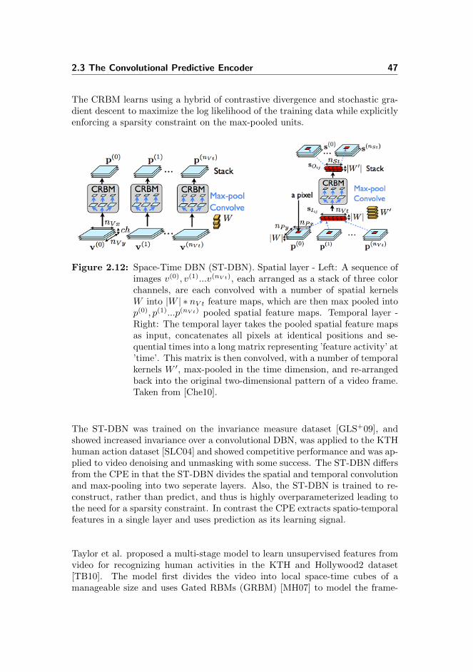
2.3 The Convolutional Predictive Encoder 47
The CRBM learns using a hybrid of contrastive divergence and stochastic gra-dient descent to maximize the log likelihood of the training data while explicitlyenforcing a sparsity constraint on the max-pooled units.
Figure 2.12: Space-Time DBN (ST-DBN). Spatial layer - Left: A sequence ofimages v(0), v(1)...v(nV t), each arranged as a stack of three colorchannels, are each convolved with a number of spatial kernelsW into |W | ∗ nV t feature maps, which are then max pooled intop(0), p(1)...p(nV t) pooled spatial feature maps. Temporal layer -Right: The temporal layer takes the pooled spatial feature mapsas input, concatenates all pixels at identical positions and se-quential times into a long matrix representing ’feature activity’ at’time’. This matrix is then convolved, with a number of temporalkernels W ′, max-pooled in the time dimension, and re-arrangedback into the original two-dimensional pattern of a video frame.Taken from [Che10].
The ST-DBN was trained on the invariance measure dataset [GLS+09], andshowed increased invariance over a convolutional DBN, was applied to the KTHhuman action dataset [SLC04] and showed competitive performance and was ap-plied to video denoising and unmasking with some success. The ST-DBN differsfrom the CPE in that the ST-DBN divides the spatial and temporal convolutionand max-pooling into two seperate layers. Also, the ST-DBN is trained to re-construct, rather than predict, and thus is highly overparameterized leading tothe need for a sparsity constraint. In contrast the CPE extracts spatio-temporalfeatures in a single layer and uses prediction as its learning signal.
Taylor et al. proposed a multi-stage model to learn unsupervised features fromvideo for recognizing human activities in the KTH and Hollywood2 dataset[TB10]. The model first divides the video into local space-time cubes of amanageable size and uses Gated RBMs (GRBM) [MH07] to model the frame-

2.3 The Convolutional Predictive Encoder 48
to-frame transformations. In a gated RBM, the hidden features, or so called’transformation-codes’ modulates visible frame-to-frame weights, thus allowingthe features to modulate lower level correlation between successive frames. Themodel then learns a sparse dictionary of the latent transformation-codes, whichfinally, are max-pooled and fed into a SVM for classification. The model achievescompetetive results on both the KTH dataset and the Hollywood2 dataset. TheCPE, in contrast is a simpler architecture and only uses a single building block.
Figure 2.13: The model proposed by Taylor et al. Taken from [TB10].
2.3.2 Results
In the following experiments the same dataset as for the predictive encoder wasused. This time the images were not made into patches but were resized to160x90 for computational efficiency.
The first experiment was a convolutional predictive encoder with 20 input/outputkernels (i.e. 20 feature cubes) of size (2x5x5). Conservative hyperparameterswere chosen: a fixed learning rate of 0.001, µ of 1 such that the second order

2.3 The Convolutional Predictive Encoder 49
method could not speed up learning in in flat regions of parameter space onlyslow it down in curved regions, momentum of 0.5 and a max pooling scale of(1, 1, 1) equal to no max pooling. A batchsize of 10 was chosen, and the secondorder gradients were re-calculated for every parameter update. The code wasrun for 10.000 parameter updates, giving 10.000 ∗ 10/11.116 ≈ 9 epochs whichtook around 14 hours. The results were not encouraging.
Figure 2.14: Top map of 20 output kernels of a CPE without max-pooling.All images are contrast normalized to between minus one andone.
Figure 2.14 shows the top layer of all output kernels of the trained CPE, whichcan best be described as noise. The bottom layer was equally noisy. The noisearises because the images are all very close to zero but contrast normalized tobe between -1 and 1. Several values of hyper-parameters were tried for multipleruns of similar models. None of them gave better results.
To assert whether the implementation was faulty, experiments like the ones onMNIST in [MMCS11] were created to enable comparison. The experimentsdescribed in [MMCS11] uses Convolutional Auto-Encoders (CAE) which areexactly equal to the PCE, if one does not time-shift the output cube whencalculating loss, i.e. they reconstruct, instead of predicting. CAEs are heavilyover-parameterized, as each feature map contains about as much information asthe input image. As such a CAE with a single feature map can reconstruct anyimage very well by simply copying the pixels. The non-linearities make this a bitmore complicated, but the problem remains: a CAE with K feature maps areapproximately K times over-complete [LGRN09]. Three CAEs were created andtrained on the MNIST dataset. All CAE had 20 feature maps, 20 input/outputkernels of size 5x5, µ = 1, momentum = 0.5, a fixed learning rate of 0.001,batchsize of 10 and ran for 18.000 parameter updates or 18.000 ∗ 10/60.000 =3 epochs. The code ran for approximately 1 hour. With the second ordermethod and momentum they quickly converged, and after approximately 10.000parameter updates the improvements in reconstruction were small. The secondorder gradients were re-calculated for each parameter update. The first CAEwas as described, the second was a denoising CAE, by zero-masking 50% ofthe input image pixels and the third CAE was max-pooled with a pool-size of

2.3 The Convolutional Predictive Encoder 50
2x2. In the following figures each image is contrast normalized individually tobe between minus one and one.
Figure 2.15: Left: Kernels of a CAE trained on MNIST. Right: The 20 featuremaps for a single sample.
Figure 2.16: Left: Kernels of a denoising CAE trained on MNIST. Right: The20 feature maps for a single sample.
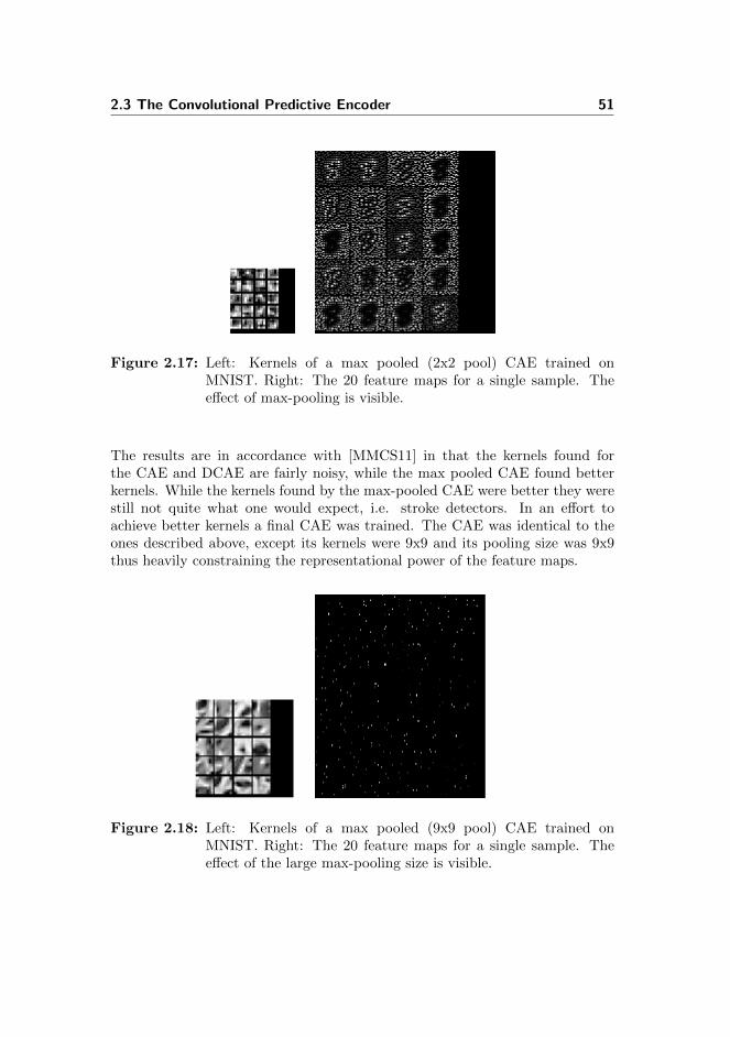
2.3 The Convolutional Predictive Encoder 51
Figure 2.17: Left: Kernels of a max pooled (2x2 pool) CAE trained onMNIST. Right: The 20 feature maps for a single sample. Theeffect of max-pooling is visible.
The results are in accordance with [MMCS11] in that the kernels found forthe CAE and DCAE are fairly noisy, while the max pooled CAE found betterkernels. While the kernels found by the max-pooled CAE were better they werestill not quite what one would expect, i.e. stroke detectors. In an effort toachieve better kernels a final CAE was trained. The CAE was identical to theones described above, except its kernels were 9x9 and its pooling size was 9x9thus heavily constraining the representational power of the feature maps.
Figure 2.18: Left: Kernels of a max pooled (9x9 pool) CAE trained onMNIST. Right: The 20 feature maps for a single sample. Theeffect of the large max-pooling size is visible.

2.3 The Convolutional Predictive Encoder 52
This finally gave good kernels resembling stroke detectors, gabor filters and bigblob detectors. The effect of the max-pooling is visible in the very sparse rep-resentation in the feature maps.
Having shown that the CPE/CAE implementation can replicate findings and,with a sufficiently large pooling, size leads to good kernels on MNIST thereare two possible reasons for the failure of the CPE. 1) the fault is in the thetime-shifting part, i.e. when using the model for prediction rather than recon-struction or 2) the data used is faulty. A third possible explanation is thatprediction is simply not a good learning signal for learning invariant features,but this would contradict the earlier findings.
To ascertain whether the fault was with the data or the time-shifting mode, aCAE, similar to the latest CAE trained on MNIST was created and trained inreconstruction mode on the the natural images. If this experiments succeededin learning good features the fault would probably be in the time-shifting partof the model, i.e. when using it for prediction. The CAE was identical topreviously described CAEs except it had 2x11x11 input/output kernel sizes anda max-pooling size of 1x10x10 as this parameter region had been shown tofind the best kernels on the MNIST dataset. The CAE was trained with moreaggressive hyperparameters of µ = 0.1, momentum = 0.9 and a fixed learningrate of 0.01. The aggressive hyperparameter settings was found to be possibleand beneficial in these heavily max-polled architectures. The results were notgood.
Figure 2.19: Weights of a CAE with 1x11x11 kernels and max-pool size of1x10x10.
The kernels look random, which is because they are all very close to zero andcontrast normalized. That the kernels are all zero are evident from the predic-tions the model made.

2.3 The Convolutional Predictive Encoder 53
Figure 2.20: Left: Correct image. Right: Predicted image.
Seeing as the results were also poor in reconstruction mode, the error probablystems from the data used. The main difference between the data used in the PEand in the CPE is that the PE works on patches cut from the original un-resizeddata, whereas the CPE works on whole, resized, images. Looking closer at theresized data it is evident that much of what was structure in the original image,resembles noise after resizing. This is probably due to the combined effect ofwhitening followed by resizing. Whitening removes local pixel correlation whilethe resizing algorithm introduces it by taking means over local regions.
Having made apparent that it was the resizing employed that caused the prob-lems a series of new experiments were run on the non-resized data. A central190x160 patch was cut out of each image, giving the same data size as previ-ously, but without the resizing problem. The series of experiments were run withspatial max-pooling sizes varying from one to four, and temporal max poolingvarying between one and two. The experiments were all run using the conserva-tive hyper-parameter setting, with 20.000 parameter updates. Each experimenttook approximately 70 hours to run. The kernels found can be seen below.
Figure 2.21: CPE kernels. No max-pooling. Top: Input kernels. Bottom:output kernels. Time goes from top to bottom.

2.3 The Convolutional Predictive Encoder 54
Figure 2.22: CPE kernels. 2x2x2 max-pooling. Top: Input kernels. Bottom:output kernels. Time goes from top to bottom.
Figure 2.23: CPE kernels. 1x2x2 max-pooling. Top: Input kernels. Bottom:output kernels. Time goes from top to bottom.
Figure 2.24: CPE kernels. 2x3x3 max-pooling. Top: Input kernels. Bottom:output kernels. Time goes from top to bottom.
Figure 2.25: CPE kernels. 1x3x3 max-pooling. Top: Input kernels. Bottom:output kernels. Time goes from top to bottom.

2.3 The Convolutional Predictive Encoder 55
Figure 2.26: CPE kernels. 2x4x4 max-pooling. Top: Input kernels. Bottom:output kernels. Time goes from top to bottom.
Figure 2.27: CPE kernels. 1x4x4 max-pooling. Top: Input kernels. Bottom:output kernels. Time goes from top to bottom.
All of the experiments has kernels showing structure, even the first experimentwithout max-pooling, although all experiments also feature seemingly noisy ker-nels. The first experiment without any max-pooling finds two gabor-like filters,a corner detector, several blob detectors and several noisy kernels. Interestinglythere is a difference in the input and output kernels; the input kernels are mostlythe same over time, whereas the output kernels changes over time. This phe-nomena can be seen in figure 2.25 the most clearly. It is evident that introducingspatial max-pooling results in better kernels, while temporal max-pooling seemsto result in slightly worse kernels. The CPE with 1x3x3 max pooling seems tofind the best kernels overall.
In order to more quantitatively evaluate the performance of the CPEs trainedthe prediction error is used. A simple baseline to compare against is using thelast shown image as the predicted output which gives a mean prediction errorof 33.79 with a standard deviation of 30.85. Table 2.1 shows the mean andstandard deviation of the prediction error on the last 1000 parameter updatesfor CPEs of varying max-pooling sizes.

2.3 The Convolutional Predictive Encoder 56
max-pool size 1x1 (s) 2x2 (s) 3x3 (s) 4x4 (s)1 (t) 19.06 (13.01) 20.43 (13.62) 20.28 (12.79) 21.53 (13.11)2 (t) 24.93 (14.54) 26.01 (14.25) 26.70 (14.27)
Table 2.1: Mean prediction error (standard deviation), of CPE for varyingsizes of spatial (s) and temporal (t) max-pooling.
All CPEs give better predictions than the baseline of just using the last inputimage as the prediction, which had a mean prediction error of 33.79. The stan-dard deviation is relatively high on all CPEs, reflecting the variety of scenesin the dataset. It is evident that the temporal max-pooling severely limits theCPE ability to make accurate predictions. This could be simply due to the factthat it has less expressive power, but the CPE with 2x2x2 max pooling has morepower than the CPE with 1x4x4 max pooling, and has worse prediction error.A single predicted frame from each model along with the frame to be predictedare shown below.
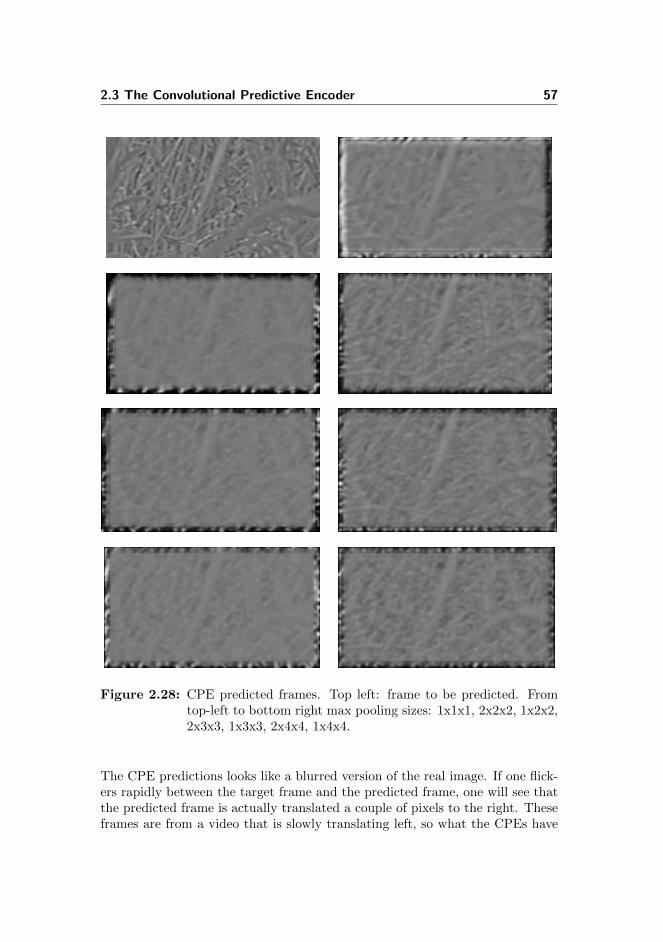
2.3 The Convolutional Predictive Encoder 57
Figure 2.28: CPE predicted frames. Top left: frame to be predicted. Fromtop-left to bottom right max pooling sizes: 1x1x1, 2x2x2, 1x2x2,2x3x3, 1x3x3, 2x4x4, 1x4x4.
The CPE predictions looks like a blurred version of the real image. If one flick-ers rapidly between the target frame and the predicted frame, one will see thatthe predicted frame is actually translated a couple of pixels to the right. Theseframes are from a video that is slowly translating left, so what the CPEs have

2.3 The Convolutional Predictive Encoder 58
done are to reconstruct a blurred version of the last input image they saw. Interms of prediction, a blurred version of the last input is not a bad strategy,but it is far from optimal. The blurred reconstruction somewhat contradicts thehighly structured kernels found.
In summary the CPE was shown to learn some structured filters, resemblinggabor filters and some noisy filters. The predictions made by the best CPEsseemed to be blurred reconstructions of the last input images they were shown.The discussion will evaluate and attempt to explain some of these findings.

Discussion
Promising findings
The prediction learning framework leads to structured filters, someresembling gabor filters
The predictive encoder and the convolutional predictive encoder trained on nat-ural video have both been shown to lead to hidden representations with receptivefields responding to structured filters, some resembling oriented gabor filters.This is the strongest finding of this thesis, as it directly supports the hypoth-esis that a simple learning rule based on minimizing prediction error works tothe degree that it can replicate receptive fields as those seen in visual areaV1. Few learning paradigms exists that have found these filters, most notableare sparse coding [OF97] including all the models using sparsity constraints,e.g. [LGRN09, LZYN11], Independent Component Analysis [vHR98] and slowfeature analysis [BW05]. This is a new paradigm, that while not perfect, hasseveral attractive properties, is biologically plausible and has a solid theoreticalfoundation.

60
Minimizing prediction error is a general, unregularized, and simplelearning rule.
The proposed architectures and learning algorithms have several attractive at-tributes. First of all the learning rule is general. It can be applied to any sensorydata, including vision, sound, touch, taste which all have a temporal componentand any imaginable man made temporal data such as weather readings (pres-sure, temperature, wind speeed, etc.), traffic flow, website usage, stock markettrends, etc.
Another very attractive property is that there was no need to regularize thealgorithm, e.g. using a sparsity constraint or limiting the hidden layer size.Instead of learning an easy task while severely limiting the model the predictionlearning framework learns a hard task without imposing any constraints on themodel. This reduces the amount of hyper-parameters and lends strength tothe core hypothesis, that prediction alone can serve as a learning signal. Asmentioned several other proposed models does not find good representationswithout being sparsity constrained. While their results are usually impressive,the need for a sparsity constraint shows that their core learning algorithm is notsufficient to find good representations. While the CPE did find better filterswhen max-pooled, the PE found good filters without any regularization with anovercomplete hidden representation. It is hypothesized that enough training ofa CPE without max-pooling would lead to similar results.
In line with not requiring any regularization the learning algorithm and ar-chitectures are relatively simple. The learning algorithm is simply stochasticgradient descent on the prediction error, implemented computationally usingthe well known back-propagation algorithm. The proposed architectures arealso relatively simple, basically being extensions into the temporal domain ofan autoencoder and a convolutional autoencoder respectively. For the CPE themore advanced stochastic diagonal levenberg-marquardt learning algorithm wasintroduced to speed up learning, but this is not a required step, it merely reduceslearning time.
The top-down predictions are useful and fit into the theoretical frame-work of biased attention.
The top down connections in the prediction learning framework are useful in twoways. First, being able to predict ones immediate sensory input is very usefulfor ones survival, such that one can avoid pain. If stacked up in a hierarchicalmanner, being able to predict high-level representations of the word might enable

61
one to predict longer-term effects of actions. From an evolutionary standpoint itis highly likely that genes enabling this kind of prediction would proliferate. It isimportant to note that while one may predict the long and short term effects ofones actions, the proposed framework does nothing to explain actually decidingwhich action to take, which implies understanding some notion of ’good’ or’bad’. But having a notion of ’good’ or ’bad’ without being able to predict theeffects of ones actions would be equally useless. Secondly it is impossible to inferthe correct configuration of the scene giving rise to the sensory inputs out of theinfinite possible configurations giving rise to the same scene without having top-down connections [Fri03]. In this light the top-down connections disambiguatehighly ambiguous sensory input, based on memory, higher order beliefs andprevious sensory input. A further strength of the proposed framework is thatthe top-down predictions fits directly in to the larger theoretical frameworks ofbiased attention and predictive coding.
The prediction learning framework has been shown to scale to fullsize images
Scaling to realistic image sizes, i.e. 200x200 pixels remains a challenging task[LGRN09], and has been identified as a key challenge for the deep learningcommunity by Andrew Ng [Ng09]. Scaling video to realistic sizes are even morechallenging due to the extra dimension of data. The CPE was shown to find somegood representations when trained on video of size 160x90 pixels. While this isnot yet realistic size video it is fairly close and provides enough information toconvey complex scenes. The use of a convolutional model was required to scaleto this level.
The proposed models can be trained layerwise and stacked into deeparchitectures
The PE and CPE were specifically designed such that they could easily bestacked into deep architectures as this have been shown to be a promising way tolearn deep hierarchical feature representations. In the case of the PE, the datawould simply be transformed into the hidden representations and the secondlayer would learn with these as their visible states. The same holds true for theCPE, where the second layer CPE would learn on the activities of the featurecubes of the first layer CPE. So far experiments have been focused on learning asingle layer of these models, in order to validate their effectiveness as a learningmodule. It remains to be shown whether they work well when stacked up.

62
Challenges
Several of the filters found are not gabor filters
The main problem is that far from all of the filters found are gabor filters.Most other models find one set of filters, i.e. blob detectors or oriented gratingsor gabor filters. The PE finds a mix of all of these, which shows that themodel is not restricted to one type of filters or the other, but instead can finda combination of filters most suitable to the task at hand. The CPE foundseveral noisy filters so it might be prudent to look at the differences of the twomodels. The key difference is in the training. The CPE was trained for muchfewer parameter updates, 20.000 compared to 10 million, using a much smallerlearning rate 0.001 compared to 0.1, though due to the second order methodand momentum, the maximum possible learning rate for the CPE was 0.004.Also every gradient step of the CPE the kernel weights were fitted to minimizeprediction error over all image positions. This is comparable to training thePE with a mini batch size of approximately (160 − 10 + 1)(90 − 10 + 1)(11 −2 + 1) = 122.310 which is quite unlike the mini batch size of 1 that was used.In effect the CPE could maximally change its weights 0.004 gradient
step 20.000 step =80 gradient, on a ”global” loss function while the PE could change its weights0.1 gradient
step 10× 106 step = 1× 10⁶ gradient on a local loss function. Further theglobal loss function is hypothesized to be much flatter due to the averaging outof nearly all gradients, while the local loss function for a single batch will havesteep parameter gradients minimizing the loss on just that patch. This mightbe one explanation as to why the PE found much better filters than the CPE.It is hypothesized that with more learning the CPE would find better kernels.
Sensitivity to max-pooling hyper-parameter
Sparsity constraints have been shown on numerous occasions to lead to gabor likefilters in models trained on natural images. As such, using a sparsity constraintwhile investigating a new models ability to extract gabor like filters from naturaldata is not optimal as any positive results could be attributed to the sparsityconstraint. For this reason the models proposed have been free of sparsityconstraints, except for the max-pooling in the CPE. The max-pooling in theCPE was used as max-pooling was shown to lead to much better filters in thestatic case when training a CAE on MNIST. Unfortunately it also proved tolead to better filters in the CPE, thus making it hard to distinguish whetherthe good filters found were due to max pooling on a noisy reconstruction task,which prediction can be approximated as, or whether it was due to minimizingprediction error. It should be noted, that while the filters are not as good, the

63
CPE without max-pooling did find gabor like filters, especially on the inputkernels. It is hypothesized that with enough training max-pooling becomes lessneeded.
Long training time
A major problem with the CPE was the prohibitively long training time. Thefinal models, which were trained for just 20.000 parameter updates took approx-imately 70 hours to train. This made debugging, trying out hyper-parametersand testing hypothesises very time consuming and a lot less flexible and easythan desired. The training time for the PE was approximately 10 times less,reflecting that the CPE processed what corresponds to 20.000 × 122.310 =2.44×10⁹ image patches, whereas the PE only processed 10×106 image patches.In this respect the CPE trained relatively faster, but the huge amount of trainingdata slowed it down.
Future research
Use Spatio-Temporally whitened data
The single most interesting observation is that the data used was not temporallywhitened. Spatial whitening is a sound pre-processing step which removes pixel-to-pixel correlations, usually found between neighbouring pixels to force themodel to find more interesting features than blob detectors. But if the datais not temporally whitened the model can simply find temporal blob detectorsand use those to good effect for reconstruction. It is hypothesized that thelack of temporal whitening has made the prediction task much easier, allowingthe models to find less spatio-temporally interesting filters and that spatio-temporally whitening the data would lead to much better filters. That spatio-temporal whitening is a sound step is supported by the finding that the humanvisual system seems to perform this exact processing [CASB09]. Running thesame experiments on spatio-temporally whitened data should be a top priorityfor future research.
Find a way to train the CPE more efficiently
As have been pointed out the training time for the CPE was excessive and thenumber of training iterations and the learning from each iteration too small.
64
Research should be directed at finding a training regime that uses less patchesper training iteration, which would lower the training time per iteration allowingmore iterations. Simple ideas include smaller images patches, i.e. 80x45 or 50x50and smaller temporal batches, e.g. 3 images per input cube instead of 11. Toscale up the model again the filters found on the smaller input cubes couldsimply be used on larger input cubes, which should work just as well as filterslearned on bigger input cubes.
Use parallel computing
To further reduce the training time the computations should be done in par-allel, ideally on a GPU or GPU cluster. Currently the computations were allrun sequentially resulting in the long training times observed. The CPE is ide-ally suited for GPU computing as 99.99% of the computational time was spentdoing convolutions, a task which can be done efficiently in parallel on a GPU,although many small convolutions are less efficiently calculated on a GPU thanfewer larger ones [AUAS+12]. A simple idea to avoid several small convolutionsis to pool them into one large convolution, and then separate out the resultsafterwards.
Evaluate the models quantitatively
If the models, after the proposed changes, consistently finds good representa-tions, experiments should be carried out that can evaluate the performanceof the models quantitatively. A natural first choice of measure would be theinvariance measure proposed by Goodfellow [GLS+09], which measures a fea-ture detectors selectivity and invariance to temporal changes. Using the modelsfor classification should be the next step. Datasets like the KTH human ac-tions dataset [SLC04] and Hollywood and Hollywood2 [MLS09] are both spatio-temporal and should serve as good benchmarks.
Investigate similarities with the denoising autoencoder
As previously mentioned the PE is comparable to a DAE, in which the addednoise is the differences between successive frames. It would be interesting tothoroughly investigate these frame-to-frame statistics to determine if they couldbe approximated with some distribution, and if using this distribution for thecorruption process in a DAE would lead to results similar to those found by thePE. This would be a good first start to answer whether the filter found by the

65
PE is a result of learning to de-noise the frame-to-frame difference distribution,or whether it is predicting the highly structured transformations taking placethat leads to good filters.
Investigate similar models
Several models close to the PE and CPE exists that would be interesting toinvestigate. A first natural choice based on the conditional RBM is a PE orCPE with visible to visible linear connections. The visible to visible connectionscould model simple correlations which would free up the top-down connections tomodel higher order dependencies. In a similar vein, and inspired by predictivecoding, the top-to-bottom connections could carry only the error signal, i.e.how wrong were the predictions made. The layer above would learn to modelthe errors made by the lower layer, effectively carrying exactly the informationneeded to make perfect predictions at lower levels in the top-down connections.

Appendix: One-Dimensionalconvolutional
back-propagation
The core equations for the convolutional neural net
a(x) = sigm
(b+
(N∑n=1
i(x− n) ik(n)
))
o(x) = sigm
(c+
(M∑m=1
a(x−m) ok(m)
))e(x) = o(x)− y(x)
L =
∑Xx=1 e(x)
2
2

67
The partial derivative for c, the output bias.
∂
∂cL =
X∑x=1
e(x)∂
∂ce(x)
∂
∂cL =
X∑x=1
e(x)∂
∂c(o(x)− y(x))
∂
∂cL =
X∑x=1
e(x) o(x) (1− o(x))∂
∂c
(c+
(M∑m=1
a(x−m) ok(m)
))∂
∂cL = −
X∑x=1
e(x) o(x) (o(x)− 1)
∂
∂cL =
X∑x=1
od(x)
The partial derivative for ok, the output kernels. Notice that a′ equals a flippedin all dimensions, i.e. reverse ordered.
∂
∂ok(m)L =
X∑x=1
od(x)∂
∂ok(m)
(c+
(M∑m=1
a(x−m) ok(m)
))∂
∂ok(m)L =
X∑x=1
a(x−m) od(x)
∂
∂ok(m)L =
X∑x=1
a′(m− x) od(x)

68
The partial derivative for b, the feature biases.
∂
∂bL =
X∑x=1
od(x)∂
∂b
(c+
(M∑m=1
a(x−m) ok(m)
))∂
∂bL =
X∑x=1
od(x)
(M∑m=1
∂
∂b(a(x−m) ok(m))
)∂
∂bL =
X∑x=1
od(x)
(M∑m=1
∂
∂bsigm
(b+
(N∑n=1
i(x− n−m) ik(n)
))ok(m)
)∂
∂bL =
X∑x=1
od(x)
(M∑m=1
a(x−m) (1− a(x−m))∂
∂b
(b+
(N∑n=1
i(x− n−m) ik(n)
))ok(m)
)∂
∂bL =
X∑x=1
(M∑m=1
od(x) a(x−m) (1− a(x−m)) ok(m)
)x′ = x−m
∂
∂bL =
X−m∑x′=1−m
(M∑m=1
od(x′ +m) a(x′) (1− a(x′)) ok(m)
)∂
∂bL =
X−m∑x′=1−m
(M∑m=1
od(x′ +m) a(x′) (1− a(x′)) ok(m)
)∂
∂bL =
X−m∑x′=1−m
a(x′) (1− a(x′))
(M∑m=1
od(x′ +m) ok(m)
)∂
∂bL =
X−m∑x′=1−m
a(x′) (1− a(x′))
(M∑m=1
od(x′ −m) ok′(m)
)∂
∂bL =
X−m∑x′=1−m
ad(x′)

69
The partial derivative for ik, the input kernels.
∂
∂ik(n)L =
X−m∑x′=1−m
(M∑m=1
od(x′ +m) a(x′) (1− a(x′))∂
∂ik(n)
(b+
(N∑n=1
i(x′ − n) ik(n)
))ok(m)
)
∂
∂ik(n)L =
X−m∑x′=1−m
(M∑m=1
od(x′ +m) a(x′) (1− a(x′)) i(x′ − n) ok(m)
)∂
∂ik(n)L =
X−m∑x′=1−m
i(x′ − n) ad(x′)
∂
∂ik(n)L =
X−m∑x′=1−m
i′(n− x′) ad(x′)

Appendix: One-Dimensionalsecond order convolutional
back-propagation
The core equations for the convolutional neural net
za(x) = b+
(N∑n=1
i(x− n) ik(n)
)a(x) = sigm(za(x))
zo(x) = c+
(M∑m=1
a(x−m) ok(m)
)o(x) = sigm(zo(x))
e(x) = o(x)− y(x)
L =
∑Xx=1 e(x)
2
2
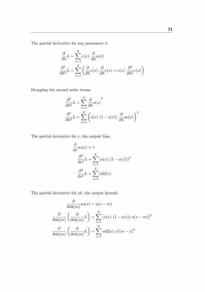
71
The partial derivative for any parameter h.
∂
∂hL =
X∑x=1
e(x)∂
∂ho(x)
∂2
∂h2L =
X∑x=1
(∂
∂he(x)
∂
∂he(x) + e(x)
∂2
∂h2e(x)
)
Dropping the second order terms.
∂2
∂h2L =
X∑x=1
∂
∂ho(x)
2
∂2
∂h2L =
X∑x=1
(o(x) (1− o(x))
∂
∂hzo(x)
)2
The partial derivative for c, the output bias.
∂
∂czo(x) = 1
∂2
∂c2L =
X∑x=1
(o(x) (1− o(x)))2
∂2
∂c2L =
X∑x=1
od2(x)
The partial derivative for ok, the output kernels.
∂
∂ok(m)zo(x) = a(x−m)
∂
∂ok(m)
(∂
∂ok(m)L
)=
X∑x=1
(o(x) (1− o(x)) a(x−m))2
∂
∂ok(m)
(∂
∂ok(m)L
)=
X∑x=1
od2(x) a′(m− x)2

72
The partial derivative for b, the feature bias.
∂
∂bzo(x) =
∂
∂b
(c+
(M∑m=1
a(x−m) ok(m)
))∂
∂ba(x−m) = a(x−m) (1− a(x−m))
∂
∂bza(x−m)
∂
∂ba(x−m) = a(x−m) (1− a(x−m))
∂
∂bzo(x) =
M∑m=1
a(x−m) (1− a(x−m)) ok(m)
∂2
∂b2L =
X∑x=1
(o(x) (1− o(x))
(M∑m=1
a(x−m) (1− a(x−m)) ok(m)
))2
∂2
∂b2L =
X∑x=1
(M∑m=1
o(x) (1− o(x)) a(x−m) (1− a(x−m)) ok(m)
)2
x′ = x−m
∂2
∂b2L =
X−m∑x′=1−m
(M∑m=1
o(x′ +m) (1− o(x′ +m)) a(x′) (1− a(x′)) ok(m)
)2
∂2
∂b2L =
X−m∑x′=1−m
(a(x′) (1− a(x′))
(M∑m=1
o(x′ +m) (1− o(x′ +m)) ok(m)
))2
∂2
∂b2L =
X−m∑x′=1−m
(a(x′) (1− a(x′)))2
(M∑m=1
od2(x′ +m) ok(m)2
)∂2
∂b2L =
X−m∑x′=1−m
(a(x′) (1− a(x′)))2
(M∑m=1
od2(x′ −m) ok′(m)2
)∂2
∂b2L =
X−m∑x′=1−m
ad2(x′)

73
The partial derivative for ik, the input kernels.
∂
∂ik(n)zo(x) =
∂
∂ik(n)
(c+
(M∑m=1
a(x−m) ok(m)
))∂
∂ik(n)zo(x) =
M∑m=1
a(x−m) (1− a(x−m))∂
∂ik(n)za(x−m)
∂
∂ik(n)zo(x) =
M∑m=1
a(x−m) (1− a(x−m)) i(x− n−m)
∂
∂ik(n)
(∂
∂ik(n)L
)=
X∑x=1
(o(x) (1− o(x))
(M∑m=1
a(x−m) (1− a(x−m)) i(x− n−m)
))2
∂
∂ik(n)
(∂
∂ik(n)L
)=
X−m∑x′=1−m
ad2(x) i(x′ − n)2
∂
∂ik(n)
(∂
∂ik(n)L
)=
X−m∑x′=1−m
ad2(x) i′(n− x′)2

Bibliography
[AB03] Alessandra Angelucci and Jean Bullier. Reaching beyond the clas-sical receptive field of V1 neurons: horizontal or feedback axons?Journal of Physiology-Paris, 97(2-3):141–154, March 2003.
[AUAS+12] Shams A. H. Al Umairy, Alexander S. Amesfoort, Irwan D. Setija,Martijn C. Beurden, and Henk J. Sips. On the Use of Small 2D Con-volutions on GPUs Computer Architecture. volume 6161 of LectureNotes in Computer Science, chapter 6, pages 52–64. Springer Berlin/ Heidelberg, Berlin, Heidelberg, 2012.
[Ben09] Yoshua Bengio. Learning Deep Architectures for AI. Foundationsand Trends R© in Machine Learning, 2(1):1–127, 2009.
[BLP+07] Yoshua Bengio, Pascal Lamblin, Dan Popovici, Hugo Larochelle,Universite De Montreal, and Montreal Quebec. Greedy layer-wisetraining of deep networks. In In NIPS, 2007.
[BM98] Dean V. Buonomano and Michael M. Merzenich. CORTICALPLASTICITY: From Synapses to Maps. Annual Review of Neuro-science, 21(1):149–186, 1998.
[Bou06] Jake Bouvrie. Notes on convolutional neural networks. Technicalreport, 2006.
[BTS+01] M. Bar, R. B. Tootell, D. L. Schacter, D. N. Greve, B. Fischl,J. D. Mendola, B. R. Rosen, and A. M. Dale. Cortical mechanismsspecific to explicit visual object recognition. Neuron, 29(2):529–535, February 2001.

BIBLIOGRAPHY 75
[Bun90] C. Bundesen. A theory of visual attention. Psychological review,97(4):523–547, October 1990.
[BW05] Pietro Berkes and Laurenz Wiskott. Slow feature analysis yieldsa rich repertoire of complex cell properties. Journal of Vision,5(6):579–602, July 2005.
[CASB09] John Cass, David Alais, Branka Spehar, and Peter J. Bex. Tempo-ral whitening: transient noise perceptually equalizes the 1/f tem-poral amplitude spectrum. Journal of vision, 9(10), 2009.
[CBB11] Aarron Courville, James Bergstra, and Yoshua Bengio. Unsuper-vised models of images by spike-and-slab rbms. In Lise Getoor andTobias Scheffer, editors, Proceedings of the 28th International Con-ference on Machine Learning (ICML-11), ICML ’11, pages 1145–1152, New York, NY, USA, June 2011. ACM.
[Che10] B. Chen. Deep learning of invariant spatio-temporal features fromvideo. 2010.
[CMS12] Dan Ciresan, Ueli Meier, and Juergen Schmidhuber. Multi-columnDeep Neural Networks for Image Classification. February 2012.
[Cre77] Otto D. Creutzfeldt. Generality of the functional structure of theneocortex. Naturwissenschaften, 64(10):507–517, October 1977.
[Dau85] John G. Daugman. Uncertainty relation for resolution in space,spatial frequency, and orientation optimized by two-dimensionalvisual cortical filters. J. Opt. Soc. Am. A, 2(7):1160–1169, July1985.
[DD95] Robert Desimone and John Duncan. Neural Mechanisms of Selec-tive Visual Attention. Annual Review of Neuroscience, 18(1):193–222, 1995.
[dVB93] J. de Villiers and E. Barnard. Backpropagation neural nets withone and two hidden layers. Neural Networks, IEEE Transactionson, 4(1):136–141, January 1993.
[EBC+10] Dumitru Erhan, Yoshua Bengio, Aaron Courville, Pierre-AntoineManzagol, Pascal Vincent, and Samy Bengio. Why Does Unsu-pervised Pre-training Help Deep Learning? Journal of MachineLearning Research, 2010.
[EGHP98] E. R. Ergenzinger, M. M. Glasier, J. O. Hahm, and T. P. Pons.Cortically induced thalamic plasticity in the primate somatosensorysystem. Nature neuroscience, 1(3):226–229, July 1998.

BIBLIOGRAPHY 76
[F91] Peter Foldiak. Learning invariance from transformation sequences.Neural Comput., 3(2):194–200, June 1991.
[Fri03] Karl Friston. Learning and inference in the brain. Neural Networks,16(9):1325–1352, November 2003.
[FVE91] Daniel J. Felleman and David C. Van Essen. Distributed Hierar-chical Processing in the Primate Cerebral Cortex. Cerebral Cortex,1(1):1–47, January 1991.
[GCR+96] J. L. Gallant, C. E. Connor, S. Rakshit, J. W. Lewis, and D. C.Van Essen. Neural responses to polar, hyperbolic, and Cartesiangratings in area V4 of the macaque monkey. Journal of neurophys-iology, 76(4):2718–2739, October 1996.
[GHB07] H. T. Ghashghaei, C. C. Hilgetag, and H. Barbas. Sequence ofinformation processing for emotions based on the anatomic dialoguebetween prefrontal cortex and amygdala. NeuroImage, 34(3):905–923, February 2007.
[GLS+09] Ian J. Goodfellow, Quoc V. Le, Andrew M. Saxe, Honglak Lee, andAndrew Y. Ng. Measuring Invariances in Deep Networks. 2009.
[Has86] J. Hastad. Almost optimal lower bounds for small depth circuits.In Proceedings of the eighteenth annual ACM symposium on Theoryof computing, STOC ’86, pages 6–20, New York, NY, USA, 1986.ACM.
[HB04] Jeff Hawkins and Sandra Blakeslee. On Intelligence. Times Books,October 2004.
[HOT06] Geoffrey E. Hinton, Simon Osindero, and Yee W. Teh. A fast learn-ing algorithm for deep belief nets. Neural Comput., 18(7):1527–1554, July 2006.
[HSW89] Kurt Hornik, Maxwell Stinchcombe, and Halbert White. Multi-layer feedforward networks are universal approximators. NeuralNetworks, 2(5):359–366, January 1989.
[HW62] D. H. HUBEL and T. N. WIESEL. Receptive fields, binocularinteraction and functional architecture in the cat’s visual cortex.The Journal of physiology, 160:106–154, January 1962.
[HW68] D. H. Hubel and T. N. Wiesel. Receptive fields and functionalarchitecture of monkey striate cortex. The Journal of physiology,195(1):215–243, March 1968.

BIBLIOGRAPHY 77
[KGB07] Kestutis Kveraga, Avniel S. Ghuman, and Moshe Bar. Top-downpredictions in the cognitive brain. Brain and Cognition, 65(2):145–168, November 2007.
[KM08] A. Klaser and M. Marszalek. A spatio-temporal descriptor basedon 3d-gradients. 2008.
[Kri10] Alex Krizhevsky. Convolutional deep belief networks on cifar-10.Technical report, 2010.
[KSJ00] Eric Kandel, James Schwartz, and Thomas Jessell. Principles ofNeural Science. McGraw-Hill Medical, 4 edition, January 2000.
[Lap05] I. Laptev. On space-time interest points. International Journal ofComputer Vision, 64(2):107–123, 2005.
[LBBH98] Y. Lecun, L. Bottou, Y. Bengio, and P. Haffner. Gradient-basedlearning applied to document recognition. Proceedings of the IEEE,86(11):2278–2324, November 1998.
[LBOM98] Y. Lecun, L. Bottou, G. B. Orr, and K. R. Muller. Efficient Back-Prop. In G. Orr and K. Muller, editors, Neural Networks—Tricksof the Trade, volume 1524 of Lecture Notes in Computer Science,pages 5–50. Springer Verlag, 1998.
[LCBD+90] Y. Le Cun, B. Boser, J. S. Denker, R. E. Howard, W. Habbard,L. D. Jackel, and D. Henderson. Advances in neural informationprocessing systems 2. chapter Handwritten digit recognition with aback-propagation network, pages 396–404. Morgan Kaufmann Pub-lishers Inc., San Francisco, CA, USA, 1990.
[LGRN09] Honglak Lee, Roger Grosse, Rajesh Ranganath, and Andrew Y.Ng. Convolutional deep belief networks for scalable unsupervisedlearning of hierarchical representations. In Proceedings of the 26thAnnual International Conference on Machine Learning, ICML ’09,pages 609–616, New York, NY, USA, 2009. ACM.
[LZYN11] Q. V. Le, W. Y. Zou, S. Y. Yeung, and A. Y. Ng. Learning hierar-chical invariant spatio-temporal features for action recognition withindependent subspace analysis. In Computer Vision and PatternRecognition (CVPR), 2011 IEEE Conference on, pages 3361–3368.IEEE, June 2011.
[MH07] R. Memisevic and G. Hinton. Unsupervised learning of image trans-formations. In Computer Vision and Pattern Recognition, 2007.CVPR’07. IEEE Conference on, pages 1–8. IEEE, 2007.

BIBLIOGRAPHY 78
[MH10] Mohamed and G. Hinton. Phone recognition using RestrictedBoltzmann Machines. In Acoustics Speech and Signal Processing(ICASSP), 2010 IEEE International Conference on, pages 4354–4357. IEEE, March 2010.
[MLS09] Marcin Marsza lek, Ivan Laptev, and Cordelia Schmid. Actionsin context. In IEEE Conference on Computer Vision & PatternRecognition, 2009.
[MMC+09] Hossein Mobahi, Hossein Mobahi, Ronan Collobert, Ronan Col-lobert, Jason Weston, and Jason Weston. Deep learning fromtemporal coherence in video. In Proceedings of the 26th AnnualInternational Conference on Machine Learning, ICML ’09, pages737–744, New York, NY, USA, 2009. ACM.
[MMCS11] Jonathan Masci, Ueli Meier, Dan Ciresan, and Jurgen Schmidhu-ber. Stacked convolutional auto-encoders for hierarchical featureextraction. In Proceedings of the 21th international conference onArtificial neural networks - Volume Part I, ICANN’11, pages 52–59,Berlin, Heidelberg, 2011. Springer-Verlag.
[Mou97] V. B. Mountcastle. The columnar organization of the neocortex.Brain : a journal of neurology, 120 ( Pt 4):701–722, April 1997.
[Ng09] Andrew Ng. Unsupervised discovery of structure, succinct repre-sentations and sparsity. In International Conference on MachineLearning, 2009.
[OF97] Bruno A. Olshausen and David J. Fieldt. Sparse coding with anovercomplete basis set: a strategy employed by V1. In VisionResearch, pages 3311–3325, 1997.
[OF04] B. Olshausen and D. Field. Sparse coding of sensory inputs. Cur-rent Opinion in Neurobiology, 14(4):481–487, August 2004.
[PCL06] Christopher Poultney, Sumit Chopra, and Yann Lecun. Efficientlearning of sparse representations with an energy-based model. InAdvances in Neural Information Processing Systems (NIPS 2006,2006.
[QvdH05] Fangtu T. Qiu and Rudiger von der Heydt. Figure and Ground inthe Visual Cortex: V2 Combines Stereoscopic Cues with GestaltRules. Neuron, 47(1):155–166, July 2005.
[RB99] Rajesh P. N. Rao and Dana H. Ballard. Predictive coding in thevisual cortex: a functional interpretation of some extra-classicalreceptive-field effects. Nature Neuroscience, 2(1):79–87, January1999.
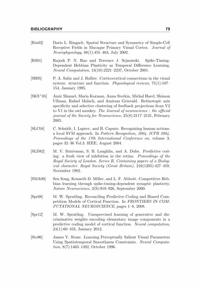
BIBLIOGRAPHY 79
[Rin02] Dario L. Ringach. Spatial Structure and Symmetry of Simple-CellReceptive Fields in Macaque Primary Visual Cortex. Journal ofNeurophysiology, 88(1):455–463, July 2002.
[RS01] Rajesh P. N. Rao and Terrence J. Sejnowski. Spike-Timing-Dependent Hebbian Plasticity as Temporal Difference Learning.Neural Computation, 13(10):2221–2237, October 2001.
[SB95] P. A. Salin and J. Bullier. Corticocortical connections in the visualsystem: structure and function. Physiological reviews, 75(1):107–154, January 1995.
[SKS+05] Amir Shmuel, Maria Korman, Anna Sterkin, Michal Harel, ShimonUllman, Rafael Malach, and Amiram Grinvald. Retinotopic axisspecificity and selective clustering of feedback projections from V2to V1 in the owl monkey. The Journal of neuroscience : the officialjournal of the Society for Neuroscience, 25(8):2117–2131, February2005.
[SLC04] C. Schuldt, I. Laptev, and B. Caputo. Recognizing human actions:a local SVM approach. In Pattern Recognition, 2004. ICPR 2004.Proceedings of the 17th International Conference on, volume 3,pages 32–36 Vol.3. IEEE, August 2004.
[SLD82] M. V. Srinivasan, S. B. Laughlin, and A. Dubs. Predictive cod-ing: a fresh view of inhibition in the retina. Proceedings of theRoyal Society of London. Series B, Containing papers of a Biolog-ical character. Royal Society (Great Britain), 216(1205):427–459,November 1982.
[SMA00] Sen Song, Kenneth D. Miller, and L. F. Abbott. Competitive Heb-bian learning through spike-timing-dependent synaptic plasticity.Nature Neuroscience, 3(9):919–926, September 2000.
[Spr08] M. W. Spratling. Reconciling Predictive Coding and Biased Com-petition Models of Cortical Function. In FRONTIERS IN COM-PUTATIONAL NEUROSCIENCE, pages 1–8, 2008.
[Spr12] M. W. Spratling. Unsupervised learning of generative and dis-criminative weights encoding elementary image components in apredictive coding model of cortical function. Neural computation,24(1):60–103, January 2012.
[Sto96] James V. Stone. Learning Perceptually Salient Visual ParametersUsing Spatiotemporal Smoothness Constraints. Neural Computa-tion, 8(7):1463–1492, October 1996.

BIBLIOGRAPHY 80
[SWB+07] Thomas Serre, Lior Wolf, Stanley Bileschi, Maximilian Riesenhu-ber, and Tomaso Poggio. Robust object recognition with cortex-likemechanisms. In IEEE Transactions on Pattern Analysis and Ma-chine Intelligence, pages 411–426, 2007.
[TB10] Graham W. Taylor and Chris Bregler. Learning local spatio-temporal features for activity recognition. Learning, 4:0–1, 2010.
[THR11] Graham W. Taylor, Geoffrey E. Hinton, and Sam T. Roweis. TwoDistributed-State Models For Generating High-Dimensional TimeSeries. Journal of Machine Learning Research, 2011.
[vHR98] J. H. van Hateren and D. L. Ruderman. Independent componentanalysis of natural image sequences yields spatio-temporal filterssimilar to simple cells in primary visual cortex. Proceedings. Biolog-ical sciences / The Royal Society, 265(1412):2315–2320, December1998.
[VLBM08] Pascal Vincent, Hugo Larochelle, Yoshua Bengio, and Pierre A.Manzagol. Extracting and composing robust features with denois-ing autoencoders. In Proceedings of the 25th international confer-ence on Machine learning, ICML ’08, pages 1096–1103, New York,NY, USA, 2008. ACM.
[VLL+10] Pascal Vincent, Hugo Larochelle, Isabelle Lajoie, Yoshua Bengio,and Pierre-Antoine Manzagol. Stacked Denoising Autoencoders:Learning Useful Representations in a Deep Network with a LocalDenoising Criterion. Journal of Machine Learning Research, 2010.
[WS02] Laurenz Wiskott and Terrence J. Sejnowski. Slow Feature Analysis:Unsupervised Learning of Invariances. 2002.
[YCC93] X. H. Yu, G. A. Chen, and S. X. Cheng. Acceleration of back-propagation learning using optimised learning rate and momentum.Electronics Letters, 29(14):1288–1290, July 1993.