Predicting Traffic Flows forTraffic Engineering inSoftware-Defined NetworksMaster-Thesis von Emmanuel StapfOktober 2016

Predicting Traffic Flows for Traffic Engineering in Software-Defined Networks

Vorgelegte Master-Thesis von Emmanuel Stapf

1. Gutachten: Prof. Dr. techn. Gerhard Neumann2. Gutachten: Patrick Jahnke

Tag der Einreichung:

Erklärung zur Master-Thesis

Hiermit versichere ich, die vorliegendeMaster-Thesis ohne Hilfe Dritter und nur mit den angegebenenQuellen und Hilfsmitteln angefertigt zu haben. Alle Stellen, die aus Quellen entnommen wurden, sindals solche kenntlich gemacht. Diese Arbeit hat in gleicher oder ähnlicher Form noch keiner Prüfungs-behörde vorgelegen.In der abgegebenen Thesis stimmen die schriftliche und elektronische Fassung überein.

Darmstadt, den 4. Oktober 2016

(Emmanuel Stapf)

AbstractTraffic congestion is a well-known problem in networks that inevitably leads to packet loss and a reduction of the networkthroughput, which in turn lowers the quality of the services running in the network. The recently emerged concept ofSoftware-Defined Networking offers unique features for implementing powerful new traffic-engineering systems to copewith the problem of network congestion. The advantages of Software-Defined Networks (SDNs) compared to traditionalnetworks arise from the presence of a central entity in the network that can obtain a global view on the current networksituation and programmatically change the routing behavior of the network devices in real time. Nevertheless, currenttraffic-engineering systems developed for SDNs cannot sufficiently prevent congestion because they only react on thecurrent network situation. The ability to predict the network traffic to a certain degree would allow a traffic-engineeringsystem to reroute the traffic before the congestion situation occurs. In previous research on network traffic prediction, realtraffic data was processed by combining many single flows and by aggregating the flows on a temporal scale. The madepredictions are inapplicable for traffic-engineering systems because they do not allow for making rerouting decisions on aper-flow basis. Furthermore, the temporal aggregation mitigates the bursty characteristics of the traffic flows. Therefore,a prediction of short high-volume traffic peaks, which are one of the main perpetrators of network congestion, is notpossible. During this master thesis, it was investigated if the prediction of single traffic flows can also be achieved whenusing flows that possess the bursty characteristics of real network traffic. For computing the predictions, the recentlydeveloped Generalized Kernel Kalman Filter [39], which embeds the formulations of the traditional Kalman Filter into aReproducing Kernel Hilbert Space, was used. The results of our prediction experiments show that by transforming thetraffic flows into the frequency domain, the peak structures of unseen flows can be predicted after learning their keycharacteristics from flows that stem from the same socket-to-socket connection.

i

Contents

1. Introduction 11.1. Thesis Structure . . . . . . . . . . . . . . . . . . . . . . . . . . . . . . . . . . . . . . . . . . . . . . . . . . . . . . . . . 2

2. Related Work 32.1. Traffic Engineering in Software-Defined Networks . . . . . . . . . . . . . . . . . . . . . . . . . . . . . . . . . . . . 32.2. Network Traffic Prediction . . . . . . . . . . . . . . . . . . . . . . . . . . . . . . . . . . . . . . . . . . . . . . . . . . . 42.3. State Estimation of Non-linear Systems . . . . . . . . . . . . . . . . . . . . . . . . . . . . . . . . . . . . . . . . . . . 5

3. Foundations 73.1. Software-Defined Networking . . . . . . . . . . . . . . . . . . . . . . . . . . . . . . . . . . . . . . . . . . . . . . . . 73.2. Time Series Modeling . . . . . . . . . . . . . . . . . . . . . . . . . . . . . . . . . . . . . . . . . . . . . . . . . . . . . 93.3. Reproducing Kernel Hilbert Space . . . . . . . . . . . . . . . . . . . . . . . . . . . . . . . . . . . . . . . . . . . . . . 11

4. Generalized Kernel Kalman Filter 154.1. RKHS Embedding of the Kalman Filter . . . . . . . . . . . . . . . . . . . . . . . . . . . . . . . . . . . . . . . . . . . 154.2. Finite-sample RKHS Embedding . . . . . . . . . . . . . . . . . . . . . . . . . . . . . . . . . . . . . . . . . . . . . . . 164.3. Sub-space GKKF . . . . . . . . . . . . . . . . . . . . . . . . . . . . . . . . . . . . . . . . . . . . . . . . . . . . . . . . . 174.4. GKKF Algorithm . . . . . . . . . . . . . . . . . . . . . . . . . . . . . . . . . . . . . . . . . . . . . . . . . . . . . . . . . 19

5. Software-Defined Network Experiment Framework 225.1. Components . . . . . . . . . . . . . . . . . . . . . . . . . . . . . . . . . . . . . . . . . . . . . . . . . . . . . . . . . . . 225.2. Workflow of the Experiment Framework . . . . . . . . . . . . . . . . . . . . . . . . . . . . . . . . . . . . . . . . . . 27

6. Traffic Prediction Experiments 306.1. Experimental Data . . . . . . . . . . . . . . . . . . . . . . . . . . . . . . . . . . . . . . . . . . . . . . . . . . . . . . . 306.2. Preprocessing the Data . . . . . . . . . . . . . . . . . . . . . . . . . . . . . . . . . . . . . . . . . . . . . . . . . . . . . 326.3. Experimental Results . . . . . . . . . . . . . . . . . . . . . . . . . . . . . . . . . . . . . . . . . . . . . . . . . . . . . . 35

7. Conclusion 40

Bibliography 41

A. Appendix 45A.1. List of Counters in OpenFlow Version 1.5.1 . . . . . . . . . . . . . . . . . . . . . . . . . . . . . . . . . . . . . . . . 45A.2. Derivation of a Finite-dimensional Kalman Gain Matrix in Hilbert Space . . . . . . . . . . . . . . . . . . . . . . 46A.3. Derivation of a Finite-dimensional Sub-space Kalman Gain Matrix in Hilbert Space . . . . . . . . . . . . . . . . 46

ii

Figures and Tables

List of Figures

3.1. Software-Defined Networking Architecture [1] . . . . . . . . . . . . . . . . . . . . . . . . . . . . . . . . . . . . . . 83.2. OpenFlow Flow Table [1] . . . . . . . . . . . . . . . . . . . . . . . . . . . . . . . . . . . . . . . . . . . . . . . . . . . 9

5.1. Architecture of the Distributed Internet Traffic Generator [2] . . . . . . . . . . . . . . . . . . . . . . . . . . . . . 235.2. Synchronized Bidirectional Flow Generation with Custom D-ITG . . . . . . . . . . . . . . . . . . . . . . . . . . . 245.3. Components and Interfaces of an Open vSwitch [3] . . . . . . . . . . . . . . . . . . . . . . . . . . . . . . . . . . . 255.4. Network Namespaces of a Virtualized Mininet Network [4] . . . . . . . . . . . . . . . . . . . . . . . . . . . . . . 255.5. MaxiNet Architecture [5] . . . . . . . . . . . . . . . . . . . . . . . . . . . . . . . . . . . . . . . . . . . . . . . . . . . 265.6. ToMaTo Web-based Editor . . . . . . . . . . . . . . . . . . . . . . . . . . . . . . . . . . . . . . . . . . . . . . . . . . . 275.7. Workflow of the Software-Defined Network Experiment Framework . . . . . . . . . . . . . . . . . . . . . . . . . 28

6.1. Application Layer Protocol Shares of TCP Traffic . . . . . . . . . . . . . . . . . . . . . . . . . . . . . . . . . . . . . 306.2. Characteristics of HTTP Flows . . . . . . . . . . . . . . . . . . . . . . . . . . . . . . . . . . . . . . . . . . . . . . . . 316.3. Segment of a Single High-volume HTTP Flow . . . . . . . . . . . . . . . . . . . . . . . . . . . . . . . . . . . . . . . 326.4. Traffic Flows of Recurring Client-Server Communication . . . . . . . . . . . . . . . . . . . . . . . . . . . . . . . . 336.5. Comparison of Data Series in Time and Frequency Domain . . . . . . . . . . . . . . . . . . . . . . . . . . . . . . 346.6. Cumulative Explained Variance per Dimension . . . . . . . . . . . . . . . . . . . . . . . . . . . . . . . . . . . . . . 356.7. Influence of Dimensionality Reduction on the Flow Appearance . . . . . . . . . . . . . . . . . . . . . . . . . . . 366.8. Prediction Results with Chunk Length 1 Second . . . . . . . . . . . . . . . . . . . . . . . . . . . . . . . . . . . . . 386.9. Chunk Length Dependent Prediction Errors . . . . . . . . . . . . . . . . . . . . . . . . . . . . . . . . . . . . . . . . 396.10.Prediction Results with Optimized Chunk Length . . . . . . . . . . . . . . . . . . . . . . . . . . . . . . . . . . . . . 39

List of Tables

6.1. Prediction Experiments Results . . . . . . . . . . . . . . . . . . . . . . . . . . . . . . . . . . . . . . . . . . . . . . . . 37

iii

Abbreviations

Notation Description

ANFIS Adaptive Neuro-Fuzzy Inference System

API Application Programming Interface

ARIMA Autoregressive Integrated Moving Average

ARMA Autoregressive Moving Average

ARP Address Resolution Protocol

BLRNN Bilinear Recurrent Neural Network

CLI Command-Line Interface

CRAM Cognitive Routing Algorithm Module

CRE Cognitive Routing Engine

DFT Discrete Fourier Transform

D-ITG Distributed Internet Traffic Generator

ECMP Equal-Cost Multi-Path

EKF Extended Kalman Filter

EM Expectation-Maximization

FFT Fast Fourier Transform

FT Fourier Transform

GARCH Generalized Autoregressive Conditional Heteroskedasticity

GKKF Generalized Kernel Kalman Filter

GRE Generic Routing Encapsulation

HMM Hidden Markov Model

HTTP Hypertext Transfer Protocol

IDT Inter Departure Time

IP Internet Protocol

JSON JavaScript Object Notation

KF Kalman Filter

KKF Kernel Kalman Filter

KKF-CEO Kernel Kalman Filter based on the Conditional Embedding Operator

KVM Kernel-based Virtual Machine

MFT Multiple Flow Tables

MLP Multilayer Perceptron

OS Operating System

OVS Open vSwitch

iv

OVSDB Open vSwitch Database Management Protocol

PC Principal Component

PCA Principal Component Analysis

QoS Quality of Service

RBF Radial Basis Function

RKHS Reproducing Kernel Hilbert Space

RNN Random Neural Network

SDN Software-Defined Network

SNMP Simple Network Management Protocol

STFT Short-Time Fourier Transform

SVM Support Vector Machine

TCP Transmission Control Protocol

TE Traffic Engineering

ToR Top of Rack

UDP User Datagram Protocol

UKF Unscented Kalman Filter

VLAN Virtual Local Area Network

VM Virtual Machine

VNC Virtual Network Computing

WAN Wide Area Network

v

1 IntroductionToday’s data centers used by private enterprises or the public sector provide a variety of applications and cloud-basedservices. Since the services differ considerably in their traffic characteristics, it is a difficult endeavor for the underpin-ning network structures to handle the traffic well during different network situations. One typical problem that arises innetworks that have to deal with large amounts of traffic is congestion. When a network device is receiving more datapackets than it can process, the packets are delayed or lost which in turn reduces the overall throughput of the network.This inevitably lowers the performance of the services and leads to a dissatisfying end-user experience.

Network protocols like the Transmission Control Protocol (TCP) provide congestion control mechanisms to cope withthe problem of traffic congestion. Whenever a packet loss is detected at the sender side of a TCP connection, a conges-tion in the network is assumed and the packet transmission rate drastically reduced. However, until the loss is noticedfrom the sender, many packets are already lost which, together with the decreased transmission rate, negatively influ-ences the quality of the provided services and lowers the network throughput.One way to deal with congestion on the hardware side is to deploy special network topologies like the fat-tree topologythat tries to prevent link overutilization by providing bigger bandwidths on links higher in the network hierarchy thatneed to transmit the aggregated traffic from the lower levels. However, providing an oversupply in bandwidth is expen-sive and as shown by Benson et al. [6], packet loss in data centers is primarily happening on links that are not heavilyutilized on average. Hence, increasing the bandwidth would not solve the problem. The reason for the losses can befound in the bursty nature of the network traffic which causes congestion when multiple traffics flows transmitted on thesame link produce high peaks simultaneously.Instead of restricting the transmission rates of single TCP connections reactively after a loss appeared, another approachwould be to spread the existing flows over the network to better exploit the provided bandwidth capacities and to miti-gate the influence of traffic bursts. Traffic Engineering (TE) systems that implement load-balancing functionalities try toachieve this by computing optimal routing paths for traffic flows. A commonly used routing strategy is Equal-Cost Multi-Path (ECMP) [7] routing which computes multiple best paths to a destination on a per-hop basis and randomly assignsflows to them. However, since the flow-to-path mapping does not take the flow sizes into account, congestion situationsstill arise in the presence of high-volume flows, called elephant-flows, because they are potentially send over the samelink. Additionally, the routing paths are static and therefore, ECMP cannot react on changing traffic characteristics.In general, traditional network architectures are not well-suited for developing sophisticated TE systems because theymiss a set of desired properties. No entity in the network is able to easily collect statistical information from all networkdevices and to aggregate them to form a global view of the network which would allow a TE application to understand thecurrent network situation and simplify the computation of routing paths. Moreover, the routing behavior in traditionalnetworks is rather static and cannot be altered programmatically on a short notice. This makes it practically impossible toreact to changing traffic characteristics. The relatively new network architecture concept of Software-Defined Network-ing possesses all the mentioned properties. Networks implementing this concept, from now on called Software-DefinedNetworks (SDNs), separate the network control from the forwarding functions of the network. The central entity isthereby represented by the SDN controller which is connected over the control plane to the network devices which inturn form the data plane. This setup allows the applications running on the controller to collect information from thenetwork devices and alter the routing behavior of the network in real time. Because of their suitability to conduct TEin them, numerous different TE systems were already developed for preventing congestion in SDNs. Yet, all approachesmeasure the current flow sizes and use this information for the path computation. Therefore, they can only react to thecurrent situation which is why congestion can not be prevented in the presence of short flow bursts.An optimal TE system would be capable of predicting the traffic flows so that a overutilization situation would be de-tected before it could be measured on the network link. Previous research on network traffic prediction mostly focusedon traffic data which was aggregated on a temporal scale and by combining many single flows. Since congestion in datacenters is caused by the interaction of short traffic bursts from elephant flows, the proposed prediction methods cannotbe utilized by potential new TE systems that aim to predict traffic flows in SDNs.

During this master thesis, it was investigated if the course of single elephant flows can be predicted on a small timescale which would allow a TE system to handle the bursty nature of network traffic in the context of congestion control.In a primary step, real-world traffic data from a university data center was analyzed in order to find structures in thediverse flow set that could be learned. Eventually, repeating structures were found for flows stemming from recurringsocket-to-socket connections. Subsequently, the selected traffic data was used in traffic prediction experiments, whereas

1

the Generalized Kernel Kalman Filter (GKKF) concept was chosen as the machine learning approach dealing with thelearning and prediction problem. The results from this master thesis can be seen as first steps in solving the task ofrevealing, if a SDN-based TE system capable of small time scale single-flow traffic prediction is feasible. Furthermore, inthe course of the prediction experiment preparation, a network experiment framework was developed which can be usedto conduct arbitrary experiments with simulated traffic and custom topologies in a scalable virtualized SDN.

1.1 Thesis Structure

In Section 2 previous research related to this master thesis is presented which includes work about TE in SDNs, theprediction of network traffic and other methods than the GKKF that can be used for state estimation in non-linearsystems. Section 3 begins with explaining the concept of Software-Defined Networking. Subsequently, the foundationsneeded for the GKKF are laid which comprise time series modeling and Reproducing Kernel Hilbert Spaces. Using thepresented foundations the formulations of the GKKF are derived in Section 4. In Section 5 the developed experimentframework used to emulate a SDN is presented by showing its components and how a typical workflow of the frameworklooks like. The results of the traffic prediction experiments using the GKKF are shown in Section 6, whereas prior to thatthe experimental data and needed preprocessing steps are described. Conclusions about the results of this master thesisare finally drawn in Section 7.

2

2 Related WorkIn the following chapter, some selected already conducted research related to this master thesis is summarized. Startingwith research on TE systems specifically designed for SDNs, followed by work on the general case of network trafficprediction. In the last section, research related to the Generalized Kernel Kalman Filter (GKKF), which was used duringthis master thesis for estimating the state of a non-linear system, is presented.

2.1 Traffic Engineering in Software-Defined Networks

The emerging network architecture concept of Software-Defined Networking possesses unique characteristics that makeSDNs well-suited for developing sophisticated TE systems. Therefore, a solid amount of research was already conductedin this area. A TE framework usually consists of a traffic measurement and a traffic management component [8]. Thetraffic measurement component collects status information from the network that could include information about thenetwork structure, its current performance or about the traffic transmitted through it. The traffic management compo-nent, which runs at the SDN controller, utilizes this information to equip the network with certain desired functionalitiesby implementing them as network services. The existing TE systems presented in this chapter focus on maximizing thethroughput of the network by providing a general load-balancing functionality in data centers or similar networks. More-over, Software-Defined Networking architectures were also used to achieve higher link utilization in Wide Area Networks(WANs) in which multiple data centers are interconnected [9, 10].

Agarwal et al. [11] showed that the problem of computing the optimal paths in a SDN that maximizes the networkthroughput can be formulated as a multi-commodity flow problem. Assuming that traffic flows can be split over multiplepaths, the resulting optimization problem can be solved in polynomial time by the controller using fully polynomial timeapproximation schemes. After the optimal paths are found, the controller forces the network devices to route the trafficflows accordingly.However, in real network scenarios computing and installing paths for every single flow can easily exceed the computa-tional capacities of the controller. Therefore, other approaches like the dynamic flow scheduling system Hedera [12] useflow information collected at the network devices to identify large flows in the network, called elephant flows, which cancause link over-utilization when sent over the same path. The central controller is calculating non-conflicting paths onlyfor those high-volume traffic flows and instructs the network devices to re-route them accordingly. Another TE systemcalled Mahout [13] is also detecting elephant flows. However, in contrast to Hedera the identification of an elephant flowis not done by polling network information from the network devices but rather at the end host sides by monitoring thehosts’ socket buffers. Thus, the overhead of control traffic sent to the central controller is reduced. Moreover, elephantflows can be detected earlier and thus, rerouting can be achieved faster. The scalable flow management tool DevoFlow[14] was designed with the same goals in mind. Here, control for smaller traffic flows is devolved back to the networkdevices. By using matching rules based on wildcards routing is directly handled by the network devices by default. Flowstatistics, which are again collected locally, are used to detect elephant flows whereas the controller is only utilized tomake re-routing decisions for those flows.Another TE system that tries to find near-optimal routing paths, while keeping the overhead of control traffic low, is theCognitive Routing Engine (CRE) [15]. Its Cognitive Routing Algorithm Module (CRAM) computes the most suitable pathsfor new flows in the network using Random Neural Networks (RNNs) together with reinforcement learning. One RNNis constructed for every network device present in the shortest path initially calculated for a new flow. CRAM makes itsdecisions upon network link characteristics. Therefore, in contrast to the TE systems described before, network informa-tion only has to be collected for every network link instead of every flow. Furthermore, the network monitoring processis optimized by storing the measured characteristics in a database for reusing and sharing them between the differentRNNs. Thus, CRE provides a TE system with a small monitoring overhead. However, the system is not focusing on largetraffic flows and therefore path computation and installation again needs to be handled by the controller for every newflow in the network.

All TE systems described share a unifying characteristic. They solely rely on network information that, in the opti-mal case, describe the current network situation and therefore, the systems can only react to those situations. As shownin [6], traffic in data centers is bursty in nature. Thus, flows switching from an OFF to an ON phase can suddenly producehigh traffic loads. If several high-volume flows peak at the same point in time this can lead to congestion in the network.In such a scenario it is not enough to start the path computation and installation process when the high traffic loads are

3

measured, because during the execution of the process data packets are already lost. Instead, it would be useful to becapable of predicting traffic flows to become aware of upcoming over-utilization situations. One TE system developedfor data centers that tries to separate the aggregated flows between Top of Rack (ToR) switch pairs or sever pairs inshort-term predictable and non-predictable flows is MicroTE [16]. For the predictable flows the controller is used tocompute optimal paths, whereas the unpredictable flows can only be routed using ECMP as a fallback routing strategy.The term predictable is used by the authors for flows whose volume does not differ from the mean traffic of the associatedToR switch pair by more then 20%. Therefore, the progression of a traffic flow is not predicted, it is just assumed that itsload will stay fairly constant in the next 1-2 seconds. The authors show that in some data centers a substantial amountof traffic remains constant on a short time scale. However, they also mention that the percentage of predictable trafficheavily depends on the applications that run in the data center. Thus, on average of all surveyed data centers only 35%of the traffic between ToR switch pairs was predictable. MicroTE is only achieving good performance when routing trafficat the finer spatial granularity of server pairs. For this scenario the authors assumed that the traffic between a serverpair is predictable if this accounts for the associated ToR switch pair. However, this might not be the case because someof the traffic consistency could be caused solely by the aggregation process. Therefore, it can be concluded that thereis a need for an actual prediction of the traffic flow progression. A TE system could use these predictions to produce aforecast on the network situation and initiate re-routing early enough to prevent link over-utilization, even in networkswith dynamic traffic patterns.

2.2 Network Traffic Prediction

As described in the last section, current TE frameworks developed for SDNs only react upon the network situation insteadof predicting its future state. However, the general case of network traffic prediction was already subject of extensiveresearch. One of most simple approaches usable to model a time series of traffic data is the Autoregressive Moving Av-erage (ARMA) model which consists of an autoregressive part performing a regression on the series of data points and amoving average part that tries to model the error of the time series. In the literature the ARMA model was used to predictnetwork traffic mostly from single applications like bit torrent [17] or file transfer applications [18]. Since the ARMAmodel is only applicable for time series produced by stationary stochastic processes, the Autoregressive Integrated Mov-ing Average (ARIMA) model was developed. It provides a generalization of the ARMA model since it can also work withdata streams from non-stationary processes by performing a differencing step on them. The ARIMA model and variantsof it were used in different scenarios for traffic prediction, e.g. in 3G mobile networks [19] or public safety networks [20].

ARMA and ARIMA models are only applicable for linear time series with constant variance. To model non-lineartime series with a time dependent variance the Generalized Autoregressive Conditional Heteroskedasticity (GARCH)model can be used. In [21] the authors showed that the model performs better than the ARIMA model in capturing thebursty nature of Internet traffic which produces a variance change over time. The group of neural networks also allowsto model non-linear time series, which is why already many different neural network types were tested for predictingnetwork traffic. In [22] e.g. dynamic Bilinear Recurrent Neural Networks (BLRNNs) were applied and showed superiorperformance compared to static BLRNNs or classical neural networks like the Multilayer Perceptron (MLP), which wereused in [23] and [24] for the prediction task. Furthermore, a special MLP variant called neural trees that allows for over-layer connections and different activation functions for different network nodes was used in [25]. Instead of applyingother neural network types, some research focused on combining neural networks with linear approaches like the ARIMAmodel because the authors assume that the traffic time series consists of linear and non-linear components [26]. Otherresearchers also connected neural networks with other system methodologies like fuzzy systems, thereby developing theAdaptive Neuro-Fuzzy Inference System (ANFIS) [27]. Moreover, also Support Vector Machines (SVMs) were used forpredicting network traffic, e.g. by Liang et al. , whereas their parameters were selected using the ant colony optimizationalgorithm [28].

The presented non-exhaustive list of related research shows that already numerous different methods were used topredict network traffic. However, none of the described approaches could be directly integrated into a TE system thataims at conducting live predicting and rerouting of traffic flows in networks like data centers on a fine-grained time andflow scale. The reason is that the used data was always aggregated in two ways.Firstly, the applied data sets mostly consisted of traffic data which was collected during a time span of days, weeks oreven months and which was aggregated on a temporal scale leading to sampling intervals for the traffic load between1 second and 1 hour. Only in [25] an interval of 0.1 seconds was used. By aggregating the traffic data in this mannerits bursty appearance is mitigated. The time series become less complex and much easier to learn. However, since fine-grained characteristics are not present in the data set anymore, they cannot be predicted, at least from the approachesperforming a high temporal aggregation. This is a problem because already rather short traffic peaks with very high loadscan cause congestion in a network, which was also observed by Benson et al. [6].

4

Secondly, the selected data was also aggregated in terms of flows, meaning that usually all independent TCP and UserDatagram Protocol (UDP) flows representing a single socket-to-socket connection were combined to one big flow. Again,this hides the bursty characteristics of the traffic and prevents the prediction of single flows. As a result, a TE systemcould not identify single high-volume flows in the network and implement a fine-grained rerouting functionality which,as shown in [16], can have a decisive influence on the performance of the TE system. Predicting single flows againcreates the need for small sampling intervals because otherwise, short high-volume flows would be represented by onlya few data points.In all of the mentioned approaches flows were split into a training and test part, therefore predictions were made basedon the history of the flows. As a result, the model for the prediction would have to be learned during the flow life timewhich is again very difficult for short high-volume flows.In contrast to the already conducted research, a different approach was examined during this master thesis. Firstly, theavailable traffic data was used at a more fine-grained level in terms of flow and sampling interval aggregation. Secondly,flows were not predicted based on their own history. Instead, entire flows with a similar structure that appeared earlierin the network served as the training data. Since the complex flow structures are produced by a process about which wehave no knowledge and whose state is not directly observable for us, the powerful concept of Hidden Markov Models(HMMs), which is described in more detail in Section 3.2.1, was utilized to model the underlying process.

2.3 State Estimation of Non-linear Systems

For predicting the upcoming load of a traffic flow in a SDN the underlying stochastic process producing the flow andforming its appearance has to be modeled and its hidden state estimated. One well-known algorithm for state estimationthat uses a HMM to model the system is the Kalman Filter (KF) [29]. However, since the KF can only be used for linearsystems, extensions like the Extended Kalman Filter (EKF) [30] and the Unscented Kalman Filter (UKF) [31] were devel-oped to allow state estimation also for non-linear systems. In the original KF the model is represented by linear functionsthat are assumed to describe the dynamics of the system. For the EKF and UKF also non-linear functions can be used formodeling the underlying process as long as they are differentiable. When computing a new state estimate with the EKFa Taylor series approximation is conducted, thereby linearizing the model around the current working point.The UKF achieves more stable and robust results using another approach. Instead of approximating the non-linear func-tions, sampling points are taken from the current state estimation given by a mean and covariance. The sampling pointsthen represent the approximated probability distribution of the state which is transformed by applying the non-linearfunctions to every point. Both the EKF and UKF assume that the non-linear functions describing the system dynamics areknown. In the setup observed during this master thesis the dynamics are unknown and therefore, other methods have tobe used.

When the model of the system is not known it has to be learned from data. However, if the true hidden states arenot present in the available data set heuristic approaches like the Expectation-Maximization (EM) algorithm are used tolearn the model. Often, these algorithms need to be carefully initialized and suffer from local optima issues. A recentapproach that allows for learning the model of a HMM without the need for hidden state information is the spectrallearning algorithm for HMMs [32]. By using the observable operator model [33], the learned HMM is modeled entirelyin observation space. As a result, the transition and observation model of the system are not explicitly recovered but aninternal representation of the hidden states is formed which is linearly related to the true representation. Under certainseparation assumptions which imply that the different observation probability distributions obtained for every discretehidden state of the system are distinct [34], the learned HMM in observation space can be used to predict future obser-vations given only a history of observations.Since the spectral learning algorithm can only be used for systems with discrete observations and hidden states, a ker-nelized version was developed by Song et al. [35] by embedding its formulation in a Reproducing Kernel Hilbert Space(RKHS). The resulting algorithm allows to utilize the advantages of spectral algorithms also for continuous state spaces.However, the assumption of distinct probability distributions is still made. The GKKF computes an uncertainty measurefor the prediction of the hidden state which is possible because the embedding of the state estimation is mapped backto the original space. The kernel spectral algorithm cannot provide a similar measure because the state estimation isrepresented by a sample in the training data that maximizes the a posteriori belief. In [36] experiments were conductedshowing that the GKKF outperforms the kernel spectral algorithm in a simulated and a real-world scenario.

Other approaches for non-linear time series modeling that are closer related to the GKKF are the Kernel Kalman Fil-ter (KKF) [37] and the Kernel Kalman Filter based on the Conditional Embedding Operator (KKF-CEO) [38]. The KKFis a kernelized version of the KF where the observations, system states and update equations of the KF are brought toa feature space by using a kernel function. However, in contrast to the GKKF a kernelized version of the system modelis only derived for the transition model but not for the observation model. As a result, the observations are computed

5

from the states simply by adding a noise term. Another difference to the GKKF is that the KF formulations are onlyembedded in a sub-space of the feature space and hence, the approach is not fully exploiting the infinite-dimensionalitycharacteristic of the feature space.The KKF-CEO embeds the formulations of the KF in a RKHS by using the conditional embedding operator which is ex-plained in more detail along with RKHSs in Section 3.3. In contrast to the KKF the KKF-CEO formulates the KF in thefull feature space provided by the kernel. Moreover, the transition model does not have to be learned using the EMalgorithm, as it is done with the KKF, but can be computed from the training data. However, as for the KKF the observa-tion model is not formulated in the RKHS and the observations again interpreted as noisy variants of the system states.Computing the transition model under this assumption using the embeddings of the noisy observations is not fully validfrom a theoretical point of view since the observations were not generated by a Markov process. Furthermore, this leadsto update equations that are farer away from the original KF equations compared to the GKKF. Besides, in [39] it wasshown that the GKKF outperforms the KKF-CEO in different experiments using data from simulated environments andreal-world applications.

6

3 FoundationsIn this chapter, the concept of Software-Defined Networking and its advantages compared to traditional network archi-tectures are described. Software-Defined Networking serves as the foundation for building the experiment frameworkintroduced in Chapter 5. Furthermore, the fundamentals needed for the GKKF from Chapter 4 are explained.

3.1 Software-Defined Networking

Software-Defined Networking is an architecture concept for networks that should enable them to meet the requirementsof modern computing environments like data centers or carrier networks. Traditional static network architectures areill-suited in this manner because they cannot cope with the dynamically changing need for memory and computingresources of today’s network services. The reasons for this change in requirements can be found, among others, in therise of cloud services, the special needs of big data applications and the change in network traffic patterns from solelyclient-server based to more machine-to-machine communication. In Section 3.1.1 the main components of a Software-Defined Networking architecture are described, followed by a more detailed view in Section 3.1.2 on how the routingbehavior in a SDN can be altered.

3.1.1 Software-Defined Networking Architecture

The core idea behind Software-Defined Networking is the separation of the network control from the forwarding func-tions of the network. A high-level view of the architecture is shown in Figure 3.1. The infrastructure layer, which is alsocalled data or forwarding layer consists of network devices that are connected following a certain topology. In traditionalnetworks the network control functionality is implemented in the network devices, making use of vendor specific operat-ing systems, applications and protocols.In a SDN the infrastructure is abstracted by moving network control to a central entity in the network, the SDN controller.The controller forms the control layer of the network and communicates over a vendor-neutral protocol with the networkdevices. The first protocol alike, called OpenFlow, is developed by the Open Network Foundation [40]. The controllercan collect statistical information from the network devices, use them in its decision making process and alter the routingbehavior of every network device, which will be further described in Section 3.1.2. As a result of the abstraction, networkdevices can remain simple and offer open interfaces to the higher layers which differs from today’s highly-specializedvendor dependent devices. Simpler network devices will reduce the overall complexity of the network and make it easierto add new devices to the network or relocate existing ones. Subsequently, networks will become more flexible and highlyscalable.The top layer is the application layer which abstracts the controller functionalities to make them callable for businessapplications. Thus, network control becomes directly programmable in a more convenient and vendor independent waywhich accelerates the development of new network services. Moreover, the centrality of the controller makes it possibleto gain a global view over the network and to use this knowledge to build applications that can alter the network behaviorin real time.

3.1.2 OpenFlow

As mentioned before, the communication between network devices and the controller is handled over the open standardprotocol OpenFlow which is implemented at both endpoints and currently available in version 1.5.1 [41]. Its main fea-tures are the extraction of statistical information from the network devices and its ability to directly manipulate theirrouting behavior.In OpenFlow all data packets transmitted over the network that match a certain set of criteria are per definition oneunique flow. As matching criteria packet properties like its destination Internet Protocol (IP) address, its source IP ad-dress, its TCP destination port and many more can be used. The filtering for these criteria is happening at the networkdevice where every unique flow is represented by an entry in a so-called flow table, which form a key element of anOpenFlow enabled network device. Flow tables, as illustrated in Figure 3.2, can be seen as a replacement for routing ta-bles in traditional devices. When a new packet is received from the device, the flow table is filtered using the match fieldsuntil a fitting entry is found. Then the specified action is executed. Using an example from Figure 3.2, the device wouldforward all packets that have the destination IP address 5.6.7.8 out of port 2. Instead of forwarding a packet to another

7

Figure 3.1.: Software-Defined Networking Architecture [1]

network device it can drop it, alter the packet values or forward it internally. The complete list of all possible actions canbe found in [41]. It is also possible to set a priority number for each entry that decides which flow entry gets picked ifmultiple ones match the criteria. Therefore, a flow table allows to program the behavior of the forwarding plane. Thiscomplete control over the forwarding functionality of the abstracted infrastructure devices makes SDNs flexible insteadof monolithic.Using one flow table per network device is simple but also very restrictive and leads to a high number of flow entries ifa more fine grained flow separation is required. This is why with OpenFlow 1.3 support for Multiple Flow Tables (MFT)was introduced. MFT allows it to build a multi-step processing model where the first flow table is used to preprocess datapackets by filtering for one property and subsequently forwarding the packet to another flow table where further match-ing and processing occurs. Thus, MFT allows to handle more interesting real-world network situations like port-basedVirtual Local Area Network (VLAN) identifiers or Virtual Routing and Forwarding [42].

Another element of OpenFlow that allows for additional packet forwarding methods are group tables to which pack-ets can be forwarded to from flow tables. Like flow tables they consist of single entries but instead of assigning only oneaction to one entry a set of so-called action buckets is defined. Every bucket can consist of several individual actionsand associated parameters. The type of a group entry decides whether all action buckets belonging to that entry areexecuted or just some of them. However, always all actions of one action bucket are executed. Group tables are veryuseful when several actions should be performed on flows like a modification of the packets followed by a forwardingaction. Moreover, group tables can also be used to split flows and forward certain shares of the flow to different ports.Thus, flows can be split over different routing paths in the network.The third type of tables in an OpenFlow enabled network device are meter tables which can be used to limit the band-width of single flows and thus, offer a simple already build-in Quality of Service (QoS) functionality. The bandwidthrates are defined in so-called meter bands together with the information on how a packet should be processed if theassociated flow exceeds that rate. Multiple meter bands can now be assigned to a single entry in the meter tableand those meter entries can in turn be assigned to flow entries. The implementation of more complex QoS applica-tions can be achieved by the combination with another OpenFlow property, namely QoS queues. Here every port of adevice can be assigned to one or multiple queues that have a certain minimum and maximum bandwidth rate configu-ration. Therefore, in contrast to the meter tables this QoS mechanism works on a per-port basis instead of a per-flow basis.

As mentioned before, another key feature of OpenFlow is the extraction of statistical information from the networkdevices which can be used by the controller applications in their decision making process. The statistical information ispresented as counters that exist for every flow table, flow entry, port, queue, group, group bucket, meter and meter band.Coming back to the example shown in Figure 3.2, whenever a packet is received from the device with the IP destinationaddress 5.6.7.8 the associated counter will be increased by one. These counters do not only exist for received packets, butalso for transmitted packets, dropped packet, packet errors and many more. The complete list of all available counters inOpenFlow can be found in Appendix A.1.

8

Figure 3.2.: OpenFlow Flow Table [1]

3.2 Time Series Modeling

The GKKF described in Chapter 4 has to deal with a time series of statistical information. For being able to makepredictions upon those series of data points the processes of the underlying system have to be modeled. The HMM whichis utilized by the GKKF for that purpose is introduced in Section 3.2.1, followed by the KF in Section 3.2.2 which formsthe foundation of the state estimation technique used in the GKKF.

3.2.1 Hidden Markov Model

The superset of Markov Models can be used to model stochastic processes were it is assumed that the process holds theMarkov property. This means that the state of the associated system, which needs to be discrete, depends only on acertain number of preceding states. Accordingly, if the current state depends only on the last state, the process is saidto possess a first-order Markov property. Depending on the setup of the system environment, different types of MarkovModels can be formulated. If the system cannot be controlled and therefore acts autonomously and if the state of thesystem is only partially observable, the used Markov Model is called Hidden Markov Model (HMM) because the true stateof the system is hidden. HMMs have been utilized in a wide range of different research fields over the last decades tosolve problems, e.g. in computational biology [43] or for pattern recognition in speeches or gestures [44, 45].

A HMM can be defined as a 5-tuple Ω = (X , Y,δ,π,λ). The state space of the system is denoted by X , whereasx t ∈ X represents the state at time point t. As described before, the true state of the system cannot be observed,only an observation emitted by the system is available and denoted by yt ∈ Y . Observations can take a discrete orcontinuous value. When assuming a first-order Markov property the state probability of x t is given by p(x t |x t−1). Thetransition probabilities between the states are described by the transition matrix δ and for the initial state by π. Theemission or observation probabilities p(yt |x t) are described by the matrix λ. Both matrices together form the parametersof the model θ = δ,λ.One of the problems usually formulated when a stochastic process is modeled by a HMM is filtering. The goal is tocalculate a probability distribution estimation of the system state p(x t |y1:t ;θ ), given only the parameters of the model θand a sequence of observations up to the current time point denoted by y1:t . The most probable state can be found bycalculating the joint probability of the current state x t and the observation sequence y1:t , which is given by the sum overthe joint probability of x t , y1:t and all possible preceding states x t−1 resulting in

p(x t , y1:t) =X∑

x t−1

p(x t , x t−1, y1:t). (3.1)

After expanding the term inside the sum by using the chain rule it can be simplified. This is possible because the assumedMarkov property of the HMM implicates that x t solely depends on x t−1 and yt therefore only on x t . The resulting recur-

9

sive formulation

p(x t , y1:t) =X∑

x t−1

p(yt |x t , x t−1, y1:t−1)p(x t |x t−1, y1:t−1)p(x t−1, y1:t−1) (3.2)

= p(yt |x t)X∑

x t−1

p(x t |x t−1)p(x t−1|y1:t−1) (3.3)

can e.g. be evaluated efficiently by making use of the forward algorithm [46]. Besides filtering another often formulatedproblem is the probability estimation of a whole state sequence p(x1:T |y1:T ;θ ) given an observation sequence and themodel parameters. This task is called decoding and the most probable sequence can again be found by calculating thejoint probability with [47]

p(x1:T , y1:T ) = p(y1:T |x1:T )p(x1:T ) (3.4)

= p(y1|x1)p(x1)T∏

t=2

p(yt |x t)p(x t |x t−1), (3.5)

which can be accomplished with the Viterbi algorithm [46].In both formulated problems, the model parameters θ were given. However, often they are not known a priori and haveto be learned from a set of training samples. A classic approach to solve this problem is the EM algorithm derived forHMMs, also known as the Baum-Welch algorithm [48]. In recent years spectral learning algorithms were developed thatdo not suffer from issues with local optima [32, 35].

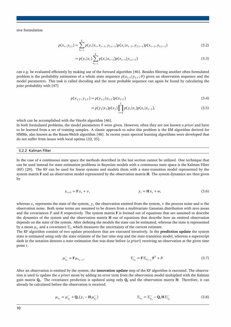
3.2.2 Kalman Filter

In the case of a continuous state space the methods described in the last section cannot be utilized. One technique thatcan be used instead for state estimation problems in Bayesian models with a continuous state space is the Kalman Filter(KF) [29]. The KF can be used for linear systems and models them with a state-transition model represented by thesystem matrix F and an observation model represented by the observation matrix H. The system dynamics are then givenby

x t+1 = F x t + v , yt = H x t +w, (3.6)

whereas x t represents the state of the system, yt the observation emitted from the system, v the process noise and w theobservation noise. Both noise terms are assumed to be drawn from a multivariate Gaussian distribution with zero meanand the covariances P and R respectively. The system matrix F is formed out of equations that are assumed to describethe dynamics of the system and the observation matrix H out of equations that describe how an emitted observationdepends on the state of the system. After defining the models the state can be estimated, whereas the state is representedby a mean µx and a covariance Σx which measures the uncertainty of the current estimate.The KF algorithm consists of two update procedures that are executed iteratively. In the prediction update the systemstate is estimated using only the state estimate of the last time step and the state-transition model, whereas a superscriptdash in the notation denotes a state estimation that was done before (a priori) receiving an observation at the given timepoint t.

µ−x t= Fµx t−1

, Σ−x t= FΣx t−1

FT + P. (3.7)

After an observation is emitted by the system, the innovation update step of the KF algorithm is executed. The observa-tion is used to update the a priori mean by adding an error term from the observation model multiplied with the Kalmangain matrix Qt. The covariance prediction is updated using only Qt and the observation matrix H. Therefore, it canalready be calculated before the observation is received.

µx t= µ−x t

+Qt (yt −Hµ−x t) Σx t

= Σ−x t−Qt HΣ−x t

(3.8)

10

The same holds for the calculation of the Kalman gain matrix. The Kalman gains can be seen as weights that decide howmuch the updated mean µx t

follows the predicted mean µ−x tor the observation yt and are calculated with

Qt = Σ−x tHT (HΣ−x t

HT + R)−1. (3.9)

The prediction and innovation update steps are usually alternated. However, it is also possible that the observationsarrive irregularly and so the state has to be predicted for several time steps in a row.As mentioned before, the KF assumes linear system dynamics which limits its usage substantially. For non-linear systemsseveral other KF variants were developed, like the EKF [30] or the UKF [31]. However, as described in Chapter 2 bothmethods require known system dynamics and do not work well for systems with high-dimensional observations. Anothermore promising group of KF variants is the one of Kernel Kalman Filters to which also the GKKF presented in Chapter 4belongs.

3.3 Reproducing Kernel Hilbert Space

Since the original KF can only deal with linear systems, the GKKF uses a kernelized KF variant which allows to conductstate estimation for systems with unknown system dynamics. This section introduces kernel methods in Section 3.3.1and reproducing kernels in Section 3.3.2 associated with RKHS. In Section 3.3.3 it is then explained how distributionscan be embedded in a RKHS. This forms an important foundation for the kernelized KF introduced in Chapter 4.

3.3.1 Kernel Methods

Kernel methods are a group of algorithms used in the field of machine learning to find structures or patterns in datasets and utilize this knowledge for solving a wide range of different tasks like classification or regression analysis. Twostate-of-the art kernel methods are support vector machines [49] and Gaussian processes [50].The unifying property that all kernel methods share is that the used data is implicitly brought from its original space toa possibly infinite-dimensional feature space. Non-linear relationships between the data points can then be representedas linear ones in the higher-order space and thus, linear algorithms can be used to learn the existing structure in thedata. Many different functions could be used for the mapping into feature space, e.g the Radial Basis Function (RBF)

φ(x) = exp

− ||x−c||2

2b2

. In the given equation x represents a data point in the original space and φ(x) its equivalent inthe feature space. The characteristics of the RBF are defined by its bandwidth b and its center c.Calculating the feature mapping explicitly, e.g. when evaluating the inner product of two feature vectors ϕ(x1)T ϕ(x2),whereas ϕ(x1)T = [φ1(x1), φ2(x1), . . . , φd(x1)], would be computationally very expensive and only possible for a fea-ture space with a finite dimension d. Instead, a kernel function can be defined which calculates the inner product withoutthe need of actually computing the mapping. Again, a scalar is returned which can be seen as a similarity measure be-tween the two input data points. One often used kernel is the Gaussian kernel which is defined as,

k(x1, x2) = ⟨ϕ(x1), ϕ(x2)⟩ (3.10)

= ϕ(x1)T ϕ(x2) (3.11)

= exp

−||x1 − x2||2

2b2

. (3.12)

This approach is called the kernel trick and allows to use a feature space with an arbitrary number of dimensions. Whenthe similarity measures should be calculated for a whole data set X = x1, x2, . . . , xm the kernel matrix Kx x ∈ Rmxm isformed,

Kx x = ΥTx Υ x =

ϕ(x1)T

...

ϕ(xm)T

× [ϕ(x1), . . . , ϕ(xm)] =

⟨ϕ(x1), ϕ(x1)⟩ · · · ⟨ϕ(x1), ϕ(xm)⟩...

. . ....

⟨ϕ(xm), ϕ(x1)⟩ · · · ⟨ϕ(xm), ϕ(xm)⟩

. (3.13)

11

In theory all valid kernel functions k(x i , x j) = ⟨ϕ(x i), ϕ(x j)⟩ are symmetric and all kernel matrices K with the elementsKi j = k(x i , x j) are positive semi-definite. Therefore, the kernel function satisfies Mercer’s condition which is

∫∫

i j

f (x i) k(x i , x j) f (x j)did j ≥ 0, (3.14)

for any squared integrable function f (x) [51]. The kernel matrix K, also called Gram matrix, then contains the innerproducts of all data point pairs.

3.3.2 Reproducing Kernels

Given a kernel function k on a data set X = x1, x2, . . . , xm defined as,

k(x i , x j) = ⟨ϕ(x i), ϕ(x j)⟩ (3.15)

= ⟨k(x i , ·), k(x j , ·)⟩ (3.16)

= ⟨kxi, kx j⟩ (3.17)

= Ki j . (3.18)

When calculating the Gram matrix K the resulting inner products form an inner product space H with an arbitrary num-ber of dimensions. If the space is complete and thus contains the inner products of all data point pairs it is called aHilbert space. The elements of the Hilbert space H can also be seen as functions f (·) = k(x , ·) = kx that produce theinner product and are approximated with the equation

f (x) =∞∑

i=1

ai k(x i , x), (3.19)

which represents a weighted sum of kernel evaluations with the weights ai ∈ R. It can now be shown with

f (x) =∞∑

i=1

ai k(x i , x) (3.20)

=

∞∑

i=1

ai kxi

T

kx (3.21)

=

®∞∑

i=1

ai kxi, kx

¸

(3.22)

= ⟨ f , kx⟩ (3.23)

that the kernel has the so-called reproducing property. By building the inner product of function f and the kernelevaluated at x , f gets reproduced, evaluated at x .As stated by the Moore–Aronszajn theorem [52], every symmetric positive definite kernel possesses the reproducingproperty and is therefore called a reproducing kernel. The associated Hilbert space is then called a Reproducing KernelHilbert Space (RKHS).

3.3.3 Embed distributions in a RKHS

One foundation for embedding the formulations of the KF in a RKHS is the capability of embedding probability densities.In the work of Smola, Gretton, Song and Schölkopf [53] an approach is described to calculate these embeddings. Fora probability density p(X ) over a random variable X the RKHS embedding is given as the expected feature mapping

12

of its random variates as µX := EX [ϕ(X )]. Whereas ϕ(X ) denotes the feature mapping of the random variable with areproducing kernel function as described in Sections 3.3.1 and 3.3.2. Usually, the underlying distribution is not knownbut a set of samples from it. The embedding of the distribution, also called mean embedding, can then be estimatedthrough a finite-sample average calculated as

µX =1m

m∑

i=1

ϕ(x i) = ΥTx 1/m. (3.24)

Furthermore, the embedding of a joint distribution p(X , Y ) is defined as the outer product of the feature mappings of therandom variates X and Y as CX Y := EX Y [ϕ(X )⊗ϕ(Y )]. The embedding can again be estimated using a finite number ofsamples from both distributions with

CX Y =1m

m∑

i=1

ϕ(x i)⊗ϕ(yi). (3.25)

Another form of distribution embedding needed for the GKKF is the embedding of a condition density defined asµY |x := EY |x[ϕ(Y )] and introduced in [54]. The embedding of the conditional distribution, given a specific value ofx , can be calculated using a conditional embedding operator CY |X with µY |x := CY |Xϕ(X ), whereas CY |X := CY X C−1

X X .Given m samples from both distributions as tuples mi = (x i , yi) the conditional embedding operator can be estimated as

CY |X = Υy (Kx x +λIm)−1 Υ T

x , (3.26)

whereas Kx x = Υ Tx Υ x denotes the Gram matrix and Υ x = [ϕ(x1), . . . , ϕ(xm)] the feature mappings of all states, as al-

ready defined in Equation 3.13. The identity matrix of size m given by Im is multiplied with the parameter λ to regularizethe Gram matrix. With the help of the conditional embedding operator, rules of probability inference like the sum rule,chain rule and Bayes’ rule can also be kernelized and used to manipulate the distributions embedded in a RKHS. Themarginal distribution of a random variable is given as p(x) =

∫

Y p(x |y) p(y)dy = EY [p(x |y)]. When embedding thedistribution p(x) by using the embedding rule for conditional distributions we end up at

µX = EX [ϕ(X )] (3.27)

= EY EX |Y [ϕ(X )] (3.28)

= EY [CX |Yϕ(Y )] (3.29)

= CX |Y EY [ϕ(Y )] (3.30)

= CX |Y µY , (3.31)

which gives us the kernelized sum rule. Thus, the conditional embedding operator CX |Y maps the embedded distributionof variable Y to the one of X . We can also use a tensor product feature to embed p(x) resulting in CX X = EX [ϕ(X )⊗ϕ(X )]and the following kernelized sum rule

CX X = EX [ϕ(X )⊗ϕ(X )] (3.32)

= EY EX |Y [ϕ(X )⊗ϕ(X )] (3.33)

= EY [C(X X )|Yϕ(Y )] (3.34)

= C(X X )|Y µY . (3.35)

With the chain rule p(x , y) = p(x |y) p(y) a joint distribution can be formulated as a product of conditional and marginaldistribution. The associated embedding CX Y := EX Y [ϕ(X )⊗ϕ(Y )] can then be factorized as

CX Y = EY [EX |Y [ϕ(X )]⊗ϕ(Y )] (3.36)

= CX |Y EY [ϕ(Y )⊗ϕ(Y )] (3.37)

= CX |Y CY Y , (3.38)

13

whereas CX Y is called the cross-covariance operator and CY Y the auto-covariance operator. By combining sum and chainrule the Bayes’ rule given as p(y|x) = p(x |y) p(y)/ p(x) can also be kernelized by

µY |x = CY |X ϕ(X ) = CX Y C−1X X ϕ(X ) (3.39)

=(CX |Y CY Y )T ϕ(X )

C(X X )|Y µY. (3.40)

14

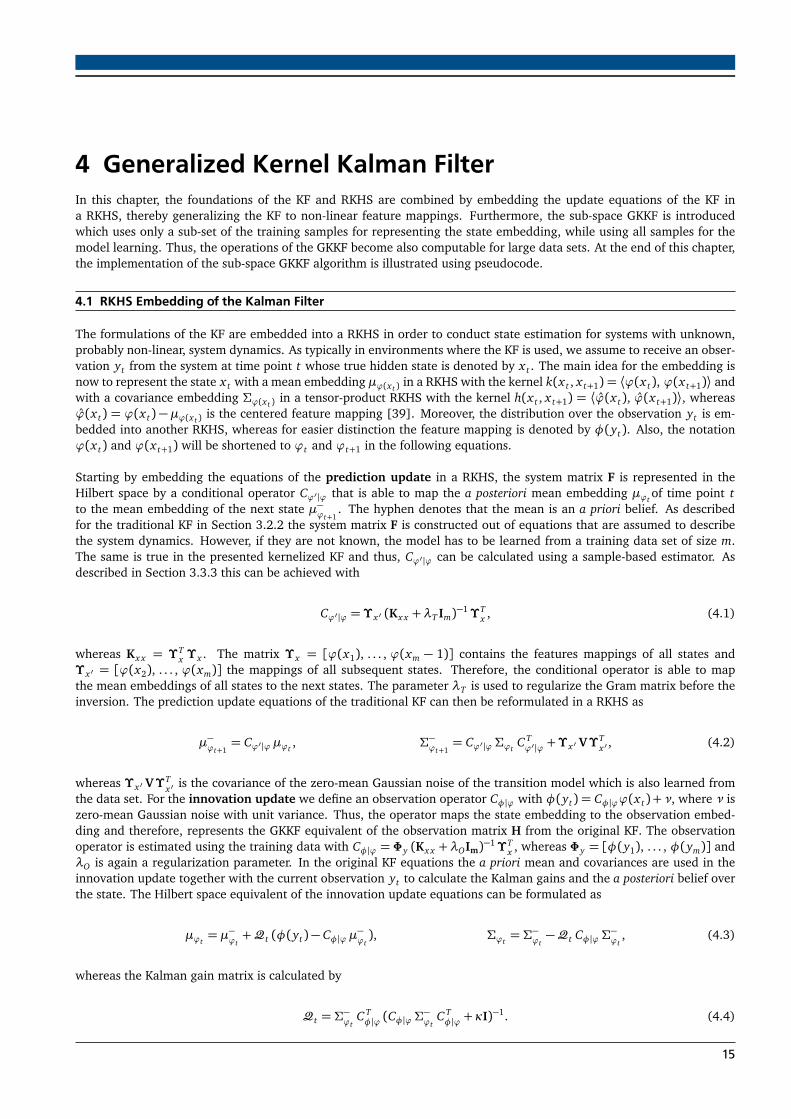
4 Generalized Kernel Kalman FilterIn this chapter, the foundations of the KF and RKHS are combined by embedding the update equations of the KF ina RKHS, thereby generalizing the KF to non-linear feature mappings. Furthermore, the sub-space GKKF is introducedwhich uses only a sub-set of the training samples for representing the state embedding, while using all samples for themodel learning. Thus, the operations of the GKKF become also computable for large data sets. At the end of this chapter,the implementation of the sub-space GKKF algorithm is illustrated using pseudocode.

4.1 RKHS Embedding of the Kalman Filter

The formulations of the KF are embedded into a RKHS in order to conduct state estimation for systems with unknown,probably non-linear, system dynamics. As typically in environments where the KF is used, we assume to receive an obser-vation yt from the system at time point t whose true hidden state is denoted by x t . The main idea for the embedding isnow to represent the state x t with a mean embedding µϕ(x t ) in a RKHS with the kernel k(x t , x t+1) = ⟨ϕ(x t), ϕ(x t+1)⟩ andwith a covariance embedding Σϕ(x t ) in a tensor-product RKHS with the kernel h(x t , x t+1) = ⟨ϕ(x t), ϕ(x t+1)⟩, whereasϕ(x t) = ϕ(x t)− µϕ(x t ) is the centered feature mapping [39]. Moreover, the distribution over the observation yt is em-bedded into another RKHS, whereas for easier distinction the feature mapping is denoted by φ(yt). Also, the notationϕ(x t) and ϕ(x t+1) will be shortened to ϕt and ϕt+1 in the following equations.

Starting by embedding the equations of the prediction update in a RKHS, the system matrix F is represented in theHilbert space by a conditional operator Cϕ′|ϕ that is able to map the a posteriori mean embedding µϕt

of time point tto the mean embedding of the next state µ−ϕt+1

. The hyphen denotes that the mean is an a priori belief. As describedfor the traditional KF in Section 3.2.2 the system matrix F is constructed out of equations that are assumed to describethe system dynamics. However, if they are not known, the model has to be learned from a training data set of size m.The same is true in the presented kernelized KF and thus, Cϕ′|ϕ can be calculated using a sample-based estimator. Asdescribed in Section 3.3.3 this can be achieved with

Cϕ′|ϕ = Υ x ′ (Kx x +λT Im)−1 Υ T

x , (4.1)

whereas Kx x = Υ Tx Υ x . The matrix Υ x = [ϕ(x1), . . . , ϕ(xm − 1)] contains the features mappings of all states and

Υ x ′ = [ϕ(x2), . . . , ϕ(xm)] the mappings of all subsequent states. Therefore, the conditional operator is able to mapthe mean embeddings of all states to the next states. The parameter λT is used to regularize the Gram matrix before theinversion. The prediction update equations of the traditional KF can then be reformulated in a RKHS as

µ−ϕt+1= Cϕ′|ϕ µϕt

, Σ−ϕt+1= Cϕ′|ϕΣϕt

C Tϕ′|ϕ + Υ x ′ VΥ

Tx ′ , (4.2)

whereas Υ x ′ VΥTx ′ is the covariance of the zero-mean Gaussian noise of the transition model which is also learned from

the data set. For the innovation update we define an observation operator Cφ|ϕ with φ(yt) = Cφ|ϕϕ(x t)+ν, where ν iszero-mean Gaussian noise with unit variance. Thus, the operator maps the state embedding to the observation embed-ding and therefore, represents the GKKF equivalent of the observation matrix H from the original KF. The observationoperator is estimated using the training data with Cφ|ϕ = Φy (Kx x +λOIm)−1 Υ T

x , whereas Φy = [φ(y1), . . . , φ(ym)] andλO is again a regularization parameter. In the original KF equations the a priori mean and covariances are used in theinnovation update together with the current observation yt to calculate the Kalman gains and the a posteriori belief overthe state. The Hilbert space equivalent of the innovation update equations can be formulated as

µϕt= µ−ϕt

+Qt (φ(yt)− Cφ|ϕ µ−ϕt), Σϕt

= Σ−ϕt−Qt Cφ|ϕΣ

−ϕt

, (4.3)

whereas the Kalman gain matrix is calculated by

Qt = Σ−ϕt

C Tφ|ϕ (Cφ|ϕΣ

−ϕt

C Tφ|ϕ + κI)−1. (4.4)

15

The zero-mean Gaussian noise of the observation model is estimated as κIm. All calculated means and covariances lie inthe Hilbert space and thus for the kernelized KF, an additional step is needed to map the embeddings back to the originalstate space. For this reconstruction of the state distribution another conditional operator CX |ϕ needs to be defined.Equivalent to the already mentioned conditional operators, it is calculated using a sample-based estimator resulting in

CX |ϕ = X (Kx x +λOIm)−1 Υ T

x , (4.5)

whereas X = [x1, . . . , xm]. The reconstruction is now conducted by applying the conditional operator to the mean andcovariance embeddings which yields

µx t= CX |ϕ µϕt

, Σx t= CX |ϕΣϕt

C TX |ϕ. (4.6)

4.2 Finite-sample RKHS Embedding

The GKKF embeds the state belief in a potentially infinite-dimensional Hilbert space. Thus, µϕtand Σϕt

cannot be com-puted directly and need to be estimated. The estimation is done by representing the mean embedding at time point tonly by a finite vector mt ∈ Rmx1 and the covariance by a finite-dimensional matrix St ∈ Rmxm through

µϕt= Υ x ′ mt , Σϕt

= Υ x ′ St ΥTx ′ . (4.7)

When inserted into the Equations 4.2 we receive a finite-sample prediction update formulation where the finite-dimensional a priori mean embedding is calculated as

µ−ϕt+1= Cϕ′|ϕ µϕt

(4.8)

Υ x ′ m−t+1 = Υ x ′ (Kx x +λT Im)

−1 Υ Tx Υ x ′ mt (4.9)

m−t+1 = (Kx x +λT Im)−1 Kx x ′mt (4.10)

= T mt . (4.11)

The transition matrix T = (Kx x + λT Im)−1 Kx x ′ is the finite-dimensional equivalent to the conditional operator Cϕ′|ϕ andforms the learned model of the underlying system’s dynamics. For the covariance embedding estimation we receive

Σ−ϕt+1= Cϕ′|ϕΣϕt

C Tϕ′|ϕ + Υ x ′ VΥ

Tx ′ (4.12)

Υ x ′ S−t+1 Υ

Tx ′ = Υ x ′ (Kx x +λT Im)

−1 Υ Tx Υ x ′ St Υ

Tx ′

Υ x ′ (Kx x +λT Im)−1 Υ T

x

T+ Υ x ′ VΥ

Tx ′ (4.13)

Υ x ′ S−t+1 Υ

Tx ′ = Υ x ′ (Kx x +λT Im)

−1 Υ Tx Υ x ′ St Υ

Tx ′ Υ x (Kx x +λT Im)

−1 Υ Tx ′ + Υ x ′ VΥ

Tx ′ (4.14)

S−t+1 = (Kx x +λT Im)−1 Kx x ′ St KT

x x ′ (Kx x +λT Im)−1 +V (4.15)

= T St TT +V. (4.16)

As a next step, the equations for a finite-sample innovation update are introduced. The finite-dimensional Kalman gainmatrix Qt ∈ Rmxm is estimated by

Qt = S−t OT (Gy y OS−t OT +κ Im)−1, (4.17)

16

whereas Gy y = ΦTy Φy is the Gram matrix of the embedded observations. The learned observation model of the un-

derlying system is given by GO = Gy yO, whereas O = (Kx x + λOIm)−1 Kx x ′ . The finite-dimensional Kalman gains canbe extracted from the infinite-dimensional ones since Qt = Υ x ′ QtΦ

Ty . All steps for deriving Qt are shown in detail in

Appendix A.2.Applying Qt , the finite-dimensional a posteriori mean embedding can be derived as

µϕt= µ−ϕt

+Qt (φ(yt)− Cφ|ϕ µ−ϕt) (4.18)

Υ x ′ mt = Υ x ′ m−t + Υ x ′ QtΦ

Ty

φ(yt)−Φy (Kx x +λOIm)−1 Υ T

x Υ x ′ m−t

(4.19)

mt = m−t +Qt (ΦTy φ(yt)−ΦT

y Φy O m−t ) (4.20)

mt = m−t +Qt (k:yt−Gy y O m−t ). (4.21)

The observations are represented by the kernel vector k:yt= [k(y1, yt), . . . , k(ym, yt)]. The finite-dimensional a posteri-

ori covariance embedding is then calculated by

Σϕt= Σ−ϕt

−Qt Cφ|ϕΣ−ϕt

(4.22)

Υ x ′ St ΥTx ′ = Υ x ′ S

−t Υ

Tx ′ − Υ x ′ QtΦ

Ty Φy (Kx x +λOIm)

−1 Υ Tx Υ x ′ S

−t Υ

Tx ′ (4.23)

St = S−t −Qt Gy y OS−t . (4.24)

As for the infinite-dimensional case, the reconstruction of the state distribution is needed to map the mean and covari-ance embeddings back to the original space. For the mean the derivations are given by

µx t= CX |ϕ µϕt

(4.25)

µx t= X (Kx x +λOIm)

−1 Υ Tx Υ x ′ mt (4.26)

= X (Kx x +λOIm)−1 Kx x ′ mt (4.27)

= X O mt (4.28)

and for the covariance by

Σx t= CX |ϕΣϕt

C TX |ϕ (4.29)

= X (Kx x +λOIm)−1 Υ T

x Υ x ′ St ΥTx ′

X (Kx x +λOIm)−1 Υ T

x

T(4.30)

= X OSt OT XT . (4.31)

4.3 Sub-space GKKF

As stated by the authors in [39], the GKKF possesses almost cubic computational complexity for the number of trainingsamples due to the inversion of the Gram matrix Kx x ∈ Rmxm. Thus, for large training sets the calculations becomepractically intractable. However, a sub-space GKKF variant can be defined that allows to work with large data sets. Thecore idea is to represent the mean embedding only by a subset of the training samples, whereas still all samples areused to learn the model. To achieve this, a sub-space feature mapping Γ x = [ϕ(x1), . . . , ϕ(xn−1)] which contains themappings of only n training samples is defined, such that Γ x ⊂ Υ x . The Gram matrix is then calculated as Kxx = Υ T

x Γ x

with dimensions Kxx ∈ Rmxn leading to new conditional embedding operators for the model learning which are calledsub-space conditional embedding operators and are introduced in [55].The formulations for the prediction update of the sub-space GKKF stay the same as for the full-space GKKF with

µ−ϕt+1= CS

ϕ′|ϕ µϕt, Σ−ϕt+1

= CSϕ′|ϕΣϕt

CSTϕ′|ϕ + Υ x ′ VΥ

Tx ′ , (4.32)

17

but the conditional operator is now given by CSϕ′|ϕ = Υ x ′ Kx x LS

T ΓTx , whereas LS

T = (KT

x x Kx x +λT In)−1.The same is true for the innovation update equations given as

µϕt= µ−ϕt

+QSt (φ(yt)− CS

φ|ϕ µ−ϕt), Σϕt

= Σ−ϕt−QS

t CSφ|ϕΣ

−ϕt

. (4.33)

Here, a sub-space conditional operator that maps the state embeddings to the observation embeddings is calculated with

CSφ|ϕ = Φy Kx x LS

O ΓTx , whereas LS

O = (KT

x x Kx x +λOIn)−1. Moreover, a sub-space Kalman gain matrix is needed that is buildusing the sub-space conditional operator. It can be computed as

QSt = Σ

−ϕt

CSTφ|ϕ (C

Sφ|ϕΣ

−ϕt

CSTφ|ϕ + κI)−1. (4.34)

Again, for the reconstruction of the state distribution a third conditional operator is needed which is calculated byCS

X |ϕ = X Kx x LSO Γ

Tx and utilized to map the feature embeddings back to the original space with the equations

µx t= CS

X |ϕ µϕt, Σx t

= CSX |ϕΣϕt

CSTX |ϕ. (4.35)

As for the full-space GKKF, the mean and covariance embeddings are possibly infinite-dimensional and need to be esti-mated to become directly computable. However, now only a subset of the training samples is used for the state represen-tation given by

nt = ΓTxµϕt

, Pt = ΓTxΣϕt

Γ x , (4.36)

whereas nt ∈ Rnx1 and Pt ∈ Rnxn. With this estimation we can formulate the finite-sample prediction update equationsfor the sub-space GKKF that allows for the computation of a finite-dimensional sub-space a priori mean embedding by

µ−ϕt+1= CS

ϕ′|ϕ µϕt(4.37)

Γ Tx µ−ϕt+1= Γ T

x Υ x ′ Kx x LST Γ

Txµϕt

(4.38)

n−t+1 = KT

x x ′ Kx x LST nt (4.39)

n−t+1 = T nt , (4.40)

whereas TS = KT

x x ′ Kx x LST is the sub-space transition matrix. For the covariance embedding estimation we end up at

Σ−ϕt+1= CS

ϕ′|ϕΣϕtCSTϕ′|ϕ + Υ x ′ VΥ

Tx ′ (4.41)

Σ−ϕt+1= Υ x ′ Kx x LS

T ΓTx Σϕt

Υ x ′ Kx x LST Γ

Tx

T+ Υ x ′ VΥ

Tx ′ (4.42)

Σ−ϕt+1= Υ x ′ Kx x LS

T ΓTx Σϕt

Γ x LST K

T

x x ΥTx ′ + Υ x ′ VΥ

Tx ′ (4.43)

Γ Tx Σ−ϕt+1Γ x = K

T

x x ′ Kx x LST Γ

Tx Σϕt

Γ x LST K

T

x x Kx x ′ + ΓTx Υ x ′ VΥ

Tx ′ Γ x (4.44)

P−t+1 = TS Pt TST + Γ Tx Υ x ′ VΥ

Tx ′ Γ x . (4.45)

For the finite-sample innovation update we start by defining a finite-dimensional sub-space Kalman gain matrix

QSt ∈ R

nxn which is estimated by QSt = P−t LS

O (KT

x x Gyy OS P−t LSO + κIn)−1 K

T

x x , whereas GOS = GyyOS with OS = Kx x LS

O isthe observation matrix. The relation to the infinite-dimensional sub-space Kalman gain matrix is given by Γ T

x QSt = QS

t ΦTy .

18

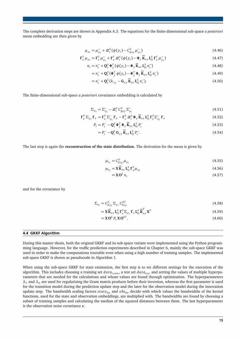
The complete derivation steps are shown in Appendix A.3. The equations for the finite-dimensional sub-space a posteriorimean embedding are then given by

µϕt= µ−ϕt

+QSt (φ(yt)− CS

φ|ϕ µ−ϕt) (4.46)

Γ Tx µϕt

= Γ Tx µ−ϕt+ Γ T

x QSt (φ(yt)−Φy Kx x LS

O ΓTx µ−ϕt) (4.47)

nt = n−t +QSt Φ

Ty (φ(yt)−Φy Kx x LS

O n−t ) (4.48)

= n−t +QSt (Φ

Ty φ(yt)−ΦT

y Φy Kx x LSO n−t ) (4.49)

= n−t +QSt (k:yt

−Gy y Kx x LSO n−t ). (4.50)

The finite-dimensional sub-space a posteriori covariance embedding is calculated by

Σϕt= Σ−ϕt

−QSt CS

φ|ϕΣ−ϕt

(4.51)

Γ Tx Σϕt

Γ x = ΓTx Σ−ϕtΓ x − Γ T

x QSt Φy Kx x LS

O ΓTxΣ−ϕtΓ x (4.52)

Pt = P−t −QSt Φ

Ty Φy Kx x LS

O P−t (4.53)

= P−t −QSt Gy y Kx x LS

O P−t . (4.54)

The last step is again the reconstruction of the state distribution. The derivation for the mean is given by

µx t= CS

X |ϕ µϕt(4.55)

µx t= X Kx x LS

O ΓTxµϕt

(4.56)

= X OS nt (4.57)

and for the covariance by

Σx t= CS

X |ϕΣϕtCST

X |ϕ (4.58)

= X Kx x LSO Γ

TxΣϕt

Γ x LSO K

T

x x XT (4.59)

= X OS Pt X OST . (4.60)

4.4 GKKF Algorithm

During this master thesis, both the original GKKF and its sub-space variant were implemented using the Python program-ming language. However, for the traffic prediction experiments described in Chapter 6, mainly the sub-space GKKF wasused in order to make the computations tractable even when using a high number of training samples. The implementedsub-space GKKF is shown as pseudocode in Algorithm 1.

When using the sub-space GKKF for state estimation, the first step is to set different settings for the execution of thealgorithm. This includes choosing a training set datat rain, a test set datatest and setting the values of multiple hyperpa-rameters that are needed for the calculations and whose values are found through optimization. The hyperparametersλT and λO are used for regularizing the Gram matrix products before their inversion, whereas the first parameter is usedfor the transition model during the prediction update step and the later for the observation model during the innovationupdate step. The bandwidth scaling factors statebw and obsbw decide with which values the bandwidths of the kernelfunctions, used for the state and observation embeddings, are multiplied with. The bandwidths are found by choosing asubset of training samples and calculating the median of the squared distances between them. The last hyperparameteris the observation noise covariance κ.

19

In the preprocess data function the training and test sets are read and prepared to be used with the GKKF algorithm.Depending on the type and structure of the used data sets different preprocessing steps might be needed. In all casesof transition and observation model learning described in this chapter, it was assumed that the training samples in factrepresent the true state x of the system. However, in some cases we might just have access to partial observations y .In such a case we can still make use of the GKKF algorithm when forming an internal state representation by using awindow of k observations yt−k+1:t , as shown in [56]. However, the formed observation windows are not a fully validrepresentation of the system state from a theoretical point of view since the observations contain additive noise and weretherefore not generated by a Markov process. When no hidden states of the system are given in the training samples,heuristic approaches like the Baum-Welch algorithm are often used to learn the model. Therefore, the authors of [39]propose to combine the Baum-Welch algorithm with the update equations of the GKKF to learn the unknown dynamicsof the system. Besides forming a state representation out of observations, the preprocess data function could includeconducting a Principal Component Analysis (PCA) on the training set to reduce the dimensions of the data sets beforeusing them with the GKKF.

Algorithm 1 Sub-space Generalized Kernel Kalman Filter

settings:training set datat raintest set datatestregularization parameters λT , λObandwidth scaling factors statebw, obsbwobservation noise covariance κ

function PREPROCESS DATA

form state windows (optional)conduct PCA on datat rain (optional)

function MODEL LEARNING

Gram matrices Kx x , Kx x ′ , Gy ystate matrix X,transition model matrix TS

observation model matrix GOS

initial belief embedding n−1 , P−1

function PROJECTION

while pro jec t doKalman gain QS

ta posteriori covariance embedding Pta priori covariance embedding P−t+1

function TEST MODEL

while predic t doif new observation yt then

innovation update:a posteriori mean embedding nt

prediction update:a priori mean embedding n−t+1

project into state space:mean prediction µx t

and covariance prediction Σx t

In the model learning function the Gram matrices of the state embeddings denoted Kx x and Kx x ′ are formed together withthe observation Gram matrix Gy y . The matrices are then used to estimate the sub-space transition model matrix TS andthe sub-space observation model matrix GOS . Moreover, the state matrix X needed for the projection back to the statespace is formed and the initial values for the a priori sub-space mean embedding n−1 and covariance embedding P−1 are set.

20

The GKKF algorithm can either be used online or offline. When used online, single observations would be omittedfrom the underlying system and directly used in the innovation update step. However, during the traffic prediction ex-periments described in Chapter 6 the algorithm was used offline, so that a complete test set datatest was already presentwhen testing the model. In the equations for the prediction and innovation updates shown in this chapter, the Kalmangain matrices and the covariances were calculated together with the mean embeddings. However, none of the com-ponents depend on the current observation yt and therefore, they can be calculated before receiving any observation.Thus, the calculation can be done in the function projection before testing the model which reduces the computationtime needed for the GKKF algorithm. For the online case, the computation of the innovation and prediction update stepsbecomes much faster which is important when the observations are received directly from the system. In the offlinemode, the projection of QS

t , Pt and P−t+1 allows to save computation time because when testing the model simultaneouslywith multiple test sets the components only have to be calculated once.

In the last step of the algorithm the model is tested, whereas the only step left in the innovation and prediction up-date is the calculation of the a posteriori and the a priori sub-space mean embeddings nt and n−t+1, respectively. After theprediction, the mean and covariance embeddings are projected back into the state space. The prediction and innovationupdate steps can be executed alternately. However, if the observations arrive irregularly only every p-th time step, thealgorithm will solely execute the prediction update step and thus perform a p-step prediction of the system state.

21

5 Software-Defined Network Experiment FrameworkOne goal during this master thesis was to create a tool that allows the user to set up a virtualized SDN and performexperiments with it. The result is the SDN experiment framework described in this chapter. It was developed using thePython programming language with the aim to execute custom experiments in custom topologies on a scalable testbed.This chapter presents the framework by introducing the different components combined in the framework, followed bya description of the steps included when starting, running and evaluating a network experiment with it.

5.1 Components

In order to build a SDN experiment framework that is scalable, multiple existing software components were combined.The first component is the Distributed Internet Traffic Generator (D-ITG) from Section 5.1.1 which is used to generatetraffic for the network experiments. The SDN itself is emulated by Mininet described in Section 5.1.3 which mainly relieson the Open vSwitch (OVS), introduced in Section 5.1.2, as its supported OpenFlow enabled virtual switch implementa-tion. To make the experiments scalable, the Mininet network is split using MaxiNet from Section 5.1.4 and executed ona set of Virtual Machines (VMs) which in turn are provided by the ToMaTo testbed described in Section 5.1.5.

5.1.1 Distributed Internet Traffic Generator

One important component of the experiment framework is the traffic generator which is used to generate network trafficflows in the emulated network. In the network experiments, single flow traces collected in real networks should bereplayed as they occurred in the real network which means that the packet timing and packet sizes should replicate thereal scenario as exact as possible.There are several traffic generators that support such a trace-based traffic generation like TCPivo [57], TCPreplay [58]or TCPopera [59]. However, because of the possibility to schedule multiple flows and the more comprehensive andconvenient way of altering properties of single flows, the traffic generator D-ITG was selected to be integrated into theexperiment framework. Furthermore, D-ITG offers more advanced features for calculating and logging network metricsand provides also an analytical model-based traffic generation mode. In this mode D-ITG is capable of producing realisticnetwork workloads that replicate stochastic processes [60]. During the experiments, this functionality was not utilizedbut might be useful in some other scenarios which is why the experiment framework becomes more flexible by integratingthe D-ITG traffic generator rather than a trace-based only generator.

An architecture overview of D-ITG is shown in Figure 5.1. The core features are provided by ITGSend and ITGRecv.ITGSend started on the sender host can run in single-flow or multi-flow mode to send flows to one or multiple differentreceiver hosts running ITGRecv. When using the multi-flow mode a new thread is spawned for every flow. Besides, a sig-naling channel is established between each couple of ITGSend and ITGRecv processes to control the traffic flows betweenthem. When ITGSend is used for trace-based traffic generation a flow is represented by a pair of files that contain thepacket size and Inter Departure Time (IDT) information for every data packet of the flow. ITGSend reads those files andreplays the flow as accurate as possible. The third possible ITGSend mode is the daemon mode. In this mode ITGSend isremotely controlled over the D-ITG Application Programming Interface (API). An example program using the interfaceis denoted as ITGManager in Figure 5.1. A similar mode is also existing for ITGRecv where it can be remotely configuredand controlled from a ITGSend component.Both ITGSend and ITGRecv can log information about every data packet they sent or received. The log files are eithercreated locally or sent to the ITGLog component located on a remote machine. After the traffic generation is finished, theITGDec component can be used to analyze the log files and to calculate flow statistics and QoS metrics like bitrate, packetloss, delay or jitter. In a subsequent step, the provided Octave script ITGplot can be used to plot the results.

When producing trace-based traffic, D-ITG can only send unidirectional flows between a sender and receiver. Tosimulate a bidirectional communication of application-level protocols, the flows need to be split into request and re-sponse parts and replayed using a ITGSend and ITGRecv instance on both the client and server side. However, as withother traffic generators, this approach is not capable of producing a truly synchronized bidirectional communication asneeded for TCP. When the main goal is to reproduce the characteristic flow patterns on the emulated links this is alsonot necessary. Though, in other scenarios this might be needed. The traffic generation platform described in [60], which

22

Figure 5.1.: Architecture of the Distributed Internet Traffic Generator [2]

is based on D-ITG, is said to support synchronized bidirectional flow generation. However, this feature is not included inthe open-source publicly available D-ITG variant. Therefore, D-ITG was extended during this master thesis by a simplemechanism illustrated in Figure 5.2 that allows for producing synchronized bidirectional TCP flows.Given an application-level flow, one host is denoted as the client and the other host as the server. Every host runs anITGSend and ITGRecv instance in parallel and owns a set of files for every flow communication it maintains to anotherhost. The files flow_idt and flow_pktz contain the IDT and packet size information for every data packet of the dedicatedflow. However, the files contain only the packets associated with the client or server side. The send_info files containtuples showing how many data packets the host has to receive before sending its own packets. The files send_idt andsend_pktz build a sending queue that contains the IDT and packet size information for packets that still need to be sendby the host. When the generation process for a flow is started the send_idt and send_pktz files are empty at the serverside and contain the information for at least one packet at the client side. The ITGSend process is constantly checkingboth files for updates. Thus, the ITGSend client instance will read the packet information and begin sending packetsto the server. The ITGRecv instance on the server side receives the packets, logs them as usual and validates, using thesend_info file, if it has to send a response in return. If not, it waits for more packets to come. If it has to send a response,the information for those packets is copied from the flow_idt and flow_pktz files to the send_idt and send_pktz files. TheITGSend instance on the server side will notice the new file content and send the appropriate packets. The same processis now happening alternately on the client and server side until the flow is finished. Since a host is always waiting for alldata packets as they occurred in the real flow before sending its own packets, this approach can only work for TCP trafficsince packets might get lost when using UDP.

5.1.2 Open vSwitch

Open vSwitch (OVS) is a multi-layer, open-source virtual switch that supports many hypervisor platforms like Kernel-based Virtual Machine (KVM) [61], Xen [62] or VirtualBox [63]. In virtual networks OVS switches act as the providerof network services for VMs which they interconnect. Since OVS was, in contrast to other virtual switch implementa-tions, designed for flexibility and general-purpose usage, it supported OpenFlow since the beginning because it makesthe switch easily re-programmable [3]. Its current version 2.5.0 supports OpenFlow up to version 1.3.The main components of OVS are shown in Figure 5.3. It consists of the processes ovsdb-server and ovs-vswitchd in theuserspace and the kernel datapath module in the kernel space, whereas the later two are involved in the data packetforwarding. Whenever a packet type is received for the first time from the virtual switch, it is directed to ovs-vswitchd.Here, it is decided how the packet should be handled making use of the different OpenFlow specific tables explained inSection 3.1.2 that were populated by the controller. The data packets are then given back to the kernel datapath moduletogether with an action that is executed and cached. Thus, a call to the userspace can be omitted for similar subsequentpackets. In this kernel version OVS does only support virtualization technologies were the kernel can be modified orextended by modules. OVS can also operate entirely in userspace without using a kernel module. However, this reducesthe performance of the switch and is at the moment declared as an experimental feature [64].The third part of OVS is the ovsdb-server. The controller uses the management protocol Open vSwitch Database Manage-ment Protocol (OVSDB) to connect to the ovsdb-server process and to configure the OVS. In contrast to OpenFlow, OVSDBis used to set more stable settings of the OVS, e.g. to add a port to the switch or to remove it.

23

Client Server

ITGRecv

ITGSend

Flow 1 to n

send_idt

send_pktz

flow_idt

flow_pktz

send_info

read

write

read

ITGRecv

ITGSend

Flow 1 to n

send_idt

send_pktz

flow_idt

flow_pktz

send_info

read

write

read

TrafficWorkload

Figure 5.2.: Synchronized Bidirectional Flow Generation with Custom D-ITG

5.1.3 Mininet

Mininet forms the basis around which the experiment framework was built. Mininet is an network emulator that allowsto rapidly prototype realistic virtual networks consisting of switches, hosts, links and controllers on a single machine [4].In contrast to the commercial network emulator EstiNet [65], Mininet is open-source. Moreover, compared to networksimulators like ns-3 [66] or OMNeT++ [67], Mininet behaves more realistic because existing applications and networkstacks are used without modifications. Mininet allows for the deployment of custom topologies and the developmentof applications implementing new network services or functionalities which makes Mininet a flexible network testbed.Because of the realistic behavior of its elements, prototypes developed in Mininet can be deployed to hardware-basedsystems with minor modifications. Furthermore, Mininet networks are interactive which means they can be managed bythe user in real-time.

Mininet uses a light-weight virtualization technique called process-based virtualization for creating a virtualized net-work. Every host and switch of the network runs in its own process but all of them lie in the same process namespace,whereas a process namespace is a container for the process state. Therefore, every node sees the same processes anddirectories and has access to the same applications installed on the underlying Operating System (OS). However, Mininetuses a Linux feature to embed the nodes in different network namespaces as illustrated in Figure 5.4. Every host is locatedin its own network namespace so that separate network interfaces, routing tables and Address Resolution Protocol (ARP)tables can be defined for every host. All switches reside in the root namespace. The links connecting the switches andhosts are realized with virtual Ethernet pairs and link parameters like bandwidth, delay or packet loss can be set by theuser. Mininet supports virtual switches like Linux bridge but also user and kernel space OpenFlow enabled switches likeOVS, whereas the current Mininet version 2.2.1 supports the newest OVS version 2.5.0. Therefore, Mininet is especiallyuseful for developing and testing applications that should run in a SDN.As shown in Figure 5.4 the controller connects over TCP to the switches, whereas it can run on the same machine or ona different machine when declared as a remote controller. As the controller, the user can either use one already includedin Mininet that implements a simple Ethernet learning switch or use any other SDN controller like Ryu [68], POX [69]or Floodlight [70] together with custom developed applications. Ryu was selected as the SDN controller implementationintegrated into the experiment framework because it supports the newest OpenFlow version 1.5.0 and like Mininet it iswritten in Python and provides a Python API.

Because of its flexibility, its ability to run with unmodified code, its support for OpenFlow enabled switches and easy-to-use Python API, Mininet appeared as the most promising network emulator to serve as the basis for the experimentframework. However, as mentioned, all Mininet components run on the same system which leads to resource limitationsbecause the resources need to be shared among the virtual hosts and switches. Besides, depending on the machineMininet is running on, other processes might also demand a share of the computation resources which can make the

24

Figure 5.3.: Components and Interfaces of an Open vSwitch [3]

experiments less repeatable. Therefore, besides using the experiment framework together with Mininet locally, it shouldallow the user to split the Mininet network between multiple machines so that it becomes more scalable. This wasachieved by using MaxiNet described in the next section.

5.1.4 MaxiNet

MaxiNet is an extension to Mininet that can be used to span an emulated network over multiple physical machines [5].In its current stable version 1.0.0 it supports Mininet version 2.2.1. An overview over the MaxiNet architecture is shownin Figure 5.5. Given an computing environment consisting of multiple physical machines in which MaxiNet is used, onemachine is declared as the Frontend, whereas the rest is denoted as Workers. The Frontend machine is the central entityused to configure and control the Mininet network by using th MaxiNet API. Internally, MaxiNet utilizes the Mininet APIto split the desired Mininet network specified by the user between the different workers, whereas also the Frontend cantake a share of the network if needed. On every Worker an unmodified Mininet instance is started, but by connecting theworkers over Generic Routing Encapsulation (GRE) tunnels the different instances act as one logical Mininet network.The user can either decide by himself which share of the Mininet network runs on which Worker or he can let MaxiNetmake the partitioning decision automatically using the graph partitioning library METIS [71]. After the network is setup, the user can interact with it over the MaxiNet Command-Line Interface (CLI) or API, almost as if he would controljust one local Mininet instance.

Figure 5.4.: Network Namespaces of a Virtualized Mininet Network [4]

25

Figure 5.5.: MaxiNet Architecture [5]

5.1.5 ToMaTo

ToMaTo stands for Topology Management Tool and is a topology-centric network testbed that is run by the ToMaTo con-sortium, an affiliation of universities and research institutes from Europe and North America. Every member contributesto the project by providing computation resources.In comparison to other experimental facility software solutions, ToMaTo offers a unique combination of features [72].A user can create virtual network topologies for their experiments that span globally over the different sites in Europeand North America. A topology can be set up using a web-based editor shown in Figure 5.6 or via the Python API ofthe back-end. ToMaTo offers two different virtual machine technologies that are used to emulate the devices of thenetwork, namely OpenVZ [73] and KVM. OpenVZ is a container-based virtualization solution, whereas KVM offers fullvirtualization by emulating all hardware needed by the guest OS. Therefore, KVM brings maximal flexibility in choosingand configuring the VMs, but it also comes at a higher cost regarding memory usage and performance reduction. Whendeciding for OpenVZ the user can select between pre-configured templates for Debian, Ubuntu or set up the devices asRyu OpenFlow controller or Floodlight OpenFlow controller. For KVM the user can select between images of Debian,Ubuntu or a pre-configured OpenFlow switch. In addition to using pre-built VMs, users can also upload their own customimages. Every VM can be accessed over Virtual Network Computing (VNC), either using client software or directly overa web-based console. Besides, ToMaTo offers network elements like switches and hubs to build the desired topology. Thelinks between the VMs are called connectors and are also emulated. This allows the user to set different link propertieslike latency or bandwidth. Furthermore, packets transmitted over the links can automatically be captured and down-loaded for later analysis. ToMaTo also offers basic monitoring functionality that enables the user to observe the resourceusage of their topologies during experiments.

The ToMaTo testbed provides the underlying computation resources for the experiment framework if the experimentsshould not be run on a local machine. Because of its flexibility in setting up custom network topologies consisting of VMsand the possibility of configuring every node in the network, ToMaTo can be used together with Mininet and MaxiNet toform a highly scalable testbed for virtualized SDNs. With this constellation the Mininet network is not necessarily splitbetween multiple physical machines, as it is usually done when used with MaxiNet, but between multiple VMs which canhowever be located on different physical machines.

26

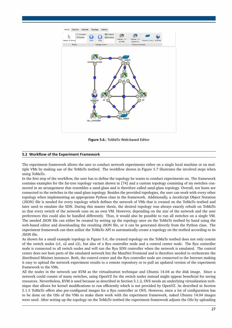
Figure 5.6.: ToMaTo Web-based Editor

5.2 Workflow of the Experiment Framework

The experiment framework allows the user to conduct network experiments either on a single local machine or on mul-tiple VMs by making use of the ToMaTo testbed. The workflow shown in Figure 5.7 illustrates the involved steps whenusing ToMaTo.In the first step of the workflow, the user has to define the topology he wants to conduct experiments on. The frameworkcontains examples for the fat-tree topology variant shown in [74] and a custom topology consisting of six switches con-nected in an arrangement that resembles a sand-glass and is therefore called sand-glass topology. Overall, ten hosts areconnected to the switches in the sand-glass topology. Besides the provided topologies, the user can work with every othertopology when implementing an appropriate Python class in the framework. Additionally, a JavaScript Object Notation(JSON) file is needed for every topology which defines the network of VMs that is created on the ToMaTo testbed andlater used to emulate the SDN. During this master thesis, the desired topology was always exactly rebuilt on ToMaToso that every switch of the network runs on an own VM. However, depending on the size of the network and the userpreferences this could also be handled differently. Thus, it would also be possible to run all switches on a single VM.The needed JSON file can either be created by setting up the topology once on the ToMaTo testbed by hand using theweb-based editor and downloading the resulting JSON file, or it can be generated directly from the Python class. Theexperiment framework can then utilize the ToMaTo API to automatically create a topology on the testbed according to itsJSON file.As shown for a small example topology in Figure 5.6, the created topology on the ToMaTo testbed does not only consistof the switch nodes (s1, s2 and s3), but also of a Ryu controller node and a control center node. The Ryu controllernode is connected to all switch nodes and will run the Ryu SDN controller when the network is emulated. The controlcenter does not host parts of the emulated network but the MaxiNet Frontend and is therefore needed to orchestrate thedistributed Mininet instances. Both, the control center and the Ryu controller node are connected to the Internet makingit easy to upload the network experiment results to a remote repository or to pull an updated version of the experimentframework to the VMs.All the nodes in the network use KVM as the virtualization technique and Ubuntu 14.04 as the disk image. Since anetwork could consist of many switches, using OpenVZ for the switch nodes instead might appear beneficial for savingresources. Nevertheless, KVM is used because as described in Section 5.1.2, OVS needs an underlying virtualization tech-nique that allows for kernel modifications to run efficiently which is not provided by OpenVZ. As described in Section5.1.5 ToMaTo offers also pre-configured images for a Ryu controller or OVS. However, since a lot of configuration hasto be done on the OSs of the VMs to make them work with the experiment framework, naked Ubuntu 14.04 imageswere used. After setting up the topology on the ToMaTo testbed the experiment framework adjusts the OSs by uploading

27

Set up Topology in ToMaTo Emulate the Network Initial Switch Configuration

Evaluate the Experiment Start the Experiment Prepare the Experiment

h1 h2

h3

s2s1

s3

define custom topology

connect VMs in ToMaTo according to JSON file

start emulated network on VMs

= define switch/host to worker mappings1

h1introducehosts to Ryu controller

h1

h2

h3

h1 h2

h3

s2

s3

calculate and implementshortest paths

s1

select flows replayed during experiment

f1.pcap f2.pcap f3.pcap

h1 h2

h3

s2

s3

f1.pcap f2.pcap

f3.pcap

prepare traffic generation

h1 h2

h3

s2

s3

f1.pcapf2.pcap

f3.pcap

generate traffic in emulated networks1

s1

use controller apps,e.g. collect statistical information

create plots from logs

control center collects plotsfrom hosts

h1

h2h3

s2s1

s3log plots

Figure 5.7.: Workflow of the Software-Defined Network Experiment Framework

configuration files and scripts to the VMs that get automatically executed. The configuration steps include installingsoftware like MaxiNet, Mininet, D-ITG and Ryu on the appropriate VMs and configuring the network interfaces. Afterthe installation process is finished, the first step of the workflow is completed and the ToMaTo topology ready to be used.

Before a SDN is emulated on the connected VMs, the framework is used to start the Ryu SDN controller togetherwith two custom applications, the network app and the monitor app. However, depending on the conducted experi-ments, other applications would need to be implemented by the user and integrated into the framework. After startingthe controller the user needs to define the MaxiNet mapping that decides which hosts and switches of the emulated net-work should run on which VM (MaxiNet Worker). Since it is not possible with MaxiNet to run also the hosts on separateVMs, they are grouped with the switch they are connected to and hosted together on a single VM. Again, this couldbe handled differently, but the mapping should fit the decisions made when setting up the VM network on the ToMaTotestbed. After the user decided for a mapping, the framework starts the network emulation by making use of MaxiNet tocreate a Mininet network and spreads it between the different VMs.

At the beginning of the third workflow step, the emulated network is up and running. However, the ARP tables ofthe hosts are still empty. The flow tables of the switches contain only one fallback flow entry which sends all data packetsthat match no other entry to the SDN controller. Those entries are installed by the network app during the start up of theemulated network when receiving messages from the switches that are sent to announce their existence. To make thehosts introduce themselves to the controller, the experiment framework forces them to ping other hosts in the network.This leads to the transmission of ARP requests that are forwarded from the switches to the controller. The network appobserves those requests and uses them to build fake ARP responses that are sent back to the hosts, thereby filling theirARP tables. Furthermore, the network app creates an internal graph of all the nodes in the emulated network and calcu-lates the shortest paths between all hosts. Then, depending on the shortest paths found, the flow tables of all switchesare populated. As a result, the hosts can now communicate, which is tested by the framework by running a ping all

28

command in the emulated network that makes all hosts ping each other.

In the next workflow step the experiment which should be run on the emulated network is prepared. Here, an ex-periment is defined as the combination of traffic that is generated in the emulated network and the custom apps thatrun on the SDN controller during the traffic generation and interact with the switches is some way. The traffic flows areselected and scheduled by the user by defining the sender and target hosts of the flows and the delays between them.Moreover, other flow properties provided by the D-ITG like the flow duration or the number of flow packets can beconfigured by the user. Additional implementations could also produce a randomized selection of flows for every host.For replaying a flow it simply needs to be provided as a .pcap file by the user. The experiment framework is then ableto prepare the traffic generation which includes reading in the .pcap files, saving them in the appropriate form at thedifferent hosts and creating additional flow dependent files needed by the D-ITG. When the user wants to send the flowsthrough a synchronized bidirectional communication, the framework e.g. has to create the different files shown in Figure5.2 which are needed for the custom D-ITG variant.During this master thesis, traffic flows were replayed in real time, thus achieving the same traffic load on the emulatedlinks as it was also present in the real network in which the flows were recorded. However, when the networks arevery large and multiple switches need to run on a single VM, or if the link bandwidth and traffic volume is very high,replaying flows in real time can become unfeasible. In such a scenario, network and traffic emulation is still possiblewhen using an approach called time dilation [75]. The idea is to make the OS and its applications believe that time ispassing at a lower speed than the actual physical time. The ratio between both perceptions of time is called the timedilation factor. When using a factor of 10 e.g., data packets that arrive at a physical rate of 1 Gbit/s appear to the OS as ifthey would arrive with 10 Gbit/s. This allows the user to study the behavior of the system at traffic speeds and capacitiesthat could otherwise not be produced with the available hardware. However, a dilation factor increases the runtime ofan experiment. Thus, generating a traffic flow with a duration of 1 minute would take 10 minutes when using a dilationfactor of 10.

The traffic generation of the experiment is initiated in the next workflow step by starting the D-ITG ITGSend and IT-GRecv processes on the hosts. During the generation, custom controller apps are used to interact with the emulatednetwork. The already mentioned monitor app was developed to periodically collect statistical information from theswitches at a certain rate. The information received from the switches include counters for the flow entries of the switchflow tables as shown in Appendix A.1. From those counters the monitor app is able to determine how much traffic eachswitch received from every connected host over a certain protocol. This is possible because the network app populatedthe flow tables with entries that allow to split the incoming traffic depending on the destination TCP or UDP port of thedata packet. It is also possible to collect those counters for every single flow that is transmitted through the switch ifthe flow entries are set accordingly. In the end, the monitor app can produce a file that contains the kbit values of singleflows or of different protocols for every host or switch of the network at a selected rate. Files produced in this mannerwere planned to serve as the data sets used for the traffic prediction experiments described in the next chapter.

In the last step, the experiment results are evaluated. During this master thesis, this mainly meant to plot the results fromthe ITGSend and ITGRecv processes to evaluate if the traffic generation was successful. Every host automatically logs itssent and received packets. After the traffic generation is finished, the experiment framework uses the ITGDec process tocreate plots out of the log files on the hosts. Afterwards, the plots are collected and stored at the control center node, sothat they can be uploaded to a repository. Moreover, the experiment framework can also collect information provided byMaxiNet which illustrate the resource utilization of the MaxiNet Workers during the experiment runtime.

29

6 Traffic Prediction ExperimentsIn the following chapter, the conducted experiments in which the GKKF was used to predict traffic flows are presented.Starting with a description of the utilized traffic data set and an explanation why a certain subset of the contained flowswas selected for forming the training and test sets. The second section shows how the data sets are preprocessed so thatthey can be used with the GKKF algorithm. The results of the experiments are then presented in the last section.

6.1 Experimental Data

The data set used during the experiments was collected as part of a study conducted by Benson et al. that aimed at analyz-ing the characteristics of network traffic in data centers [76]. During their study, Simple Network Management Protocol(SNMP) data, topology information and packet traces were collected from university, private enterprise and commercialcloud data centers. The collection of the packet traces was done by installing a sniffing tool at one or multiple switchesin each network that logged all traffic routed through the switch during a time span of 12 hours over multiple days. Afraction of the gathered packet traces of two university data centers was made publicly available by the authors [77].During this master thesis, the packet traces denoted as UNI1 were used which contain 65 minutes worth of traffic datacollected at an edge switch in a university data center consisting of 22 network devices and 500 servers. The decisionwas made for this data set because the traffic data is provided as a .pcap file. In comparison to text files, .pcap files aremore convenient when it comes to the generation of statistics on the data and the extraction of single flows from it. Foranalyzing the traffic data, the terminal-based version of Wireshark called t-shark [78] was used. Another advantage ofthe selected data set is that the traces were collected in the year 2009 which makes them considerably more current thane.g. the data sets used in [25] or [22] which date back to the mid-nineties or eighties. Selecting relatively new data isimportant because the traffic characteristics of data centers in general could have changed completely over the years andthus, insights from the experiments would not be transferable to today’s data centers.

In the first step, the packet traces were analyzed by gathering statistical information about the composition of thetraffic data. For 87% of the traffic transmitted by the observed network switch, TCP was used as the transport layerprotocol, only 13% was transmitted over UDP. A closer look on the TCP traffic then revealed which protocols were usedat the application layer. The results illustrated in Figure 6.1 show that around 90% of the overall traffic uses one of thelisted protocols, whereas Hypertext Transfer Protocol (HTTP) traffic makes up the largest share with 75%. Since the goalof this master thesis was to investigate if the progression of single flows can be predicted, we focused on traffic using thesame application layer protocol because we initially assumed that those flows would already share enough flow charac-teristics so that knowledge about some of the flows would allow us to predict other unseen ones. The decision was madein favor of HTTP traffic because this group contains 65% of all the collected traffic data. However, further analysis ofthe HTTP traffic revealed that the single HTTP flows are very heterogeneous. The packet traces contain roughly 130 000unique HTTP flows, whereas one flow represents a socket-to-socket connection between two hosts in the data center that

Figure 6.1.: Application Layer Protocol Shares of TCP Traffic

30

(a) Duration of HTTP flows (b) Traffic Load Shares of Duration Groups

Figure 6.2.: Characteristics of HTTP Flows

starts with a TCP handshake and ends with a TCP teardown. As shown in Figure 6.2a, the durations among HTTP flowsis highly diverse, whereas most of the flows are very short with a length between 0.1 and 1 second, as indicated by thered slice of the pie chart. To fully grasp the characteristics of HTTP flows it is important to know which share of thetraffic load is caused by which duration group. This information is given in Figure 6.2b and together with Figure 6.2a itallows us to gain some interesting insights. The extremely short flows with a duration of up to 0.1 seconds cause only 2%of the traffic and can therefore be neglected. The same accounts for many flows in the duration group 0.1 to 1 second,though not for all of them. The most important group seems to be the one which contains flows with a rather shortlength between 1 and 100 seconds, since only 22% of the flows possess such a length and still they cause 60% of thetraffic. All of these traffic flows could not be considered when aggregating the flows in a way as it was done in the relatedwork described in Section 2.2 since the flows would only be represented by one or a few data points. Just the flowslonger than 100 seconds could be represented sufficiently. As Figure 6.2b indicates, this duration group is responsiblefor 20% of the traffic. However, when examining the progression of high-volume long-living flows a typical flow patternis observed. One example flow is shown in Figure 6.3a which clearly reveals the extremely bursty nature of the networktraffic. Even though an already rather low sampling interval of 1 second is used, no flow structure can be observed sincethe short but very high peaks are only represented by one or two data points. For most of the time, the kbit values of theflow are either zero or have an insignificant value. This shows that even the long flows often just consist of short trafficpeaks with long low-volume phases between them. For a TE system that tries to predict and reroute traffic in a networkthis means that it needs to be able to predict the flows on a small time scale because most of the traffic is transmittedin short high-volume traffic peaks. This also implies that the traffic data must be represented using a small samplinginterval. Figure 6.3b shows the first 5 seconds of the same flow, however this time, a sampling interval of 0.01 secondswas used and now much more information about the peak structure can be obtained. As we can see, a peak itself consistsof shorter peaks which from now on are called peak impulses. At the lowest possible sampling interval these impulseswould represent single packets of the flows. In the vast majority of flows, the peaks consist of a rising phase in whichthe peak impulses gradually increase up to a certain maximum kbit value and a peak body where the traffic load ratherremains constant. In the context of network congestion the rising phase is the most interesting part of the flow becausehere the traffic pattern of the flow is changing rapidly which causes the congestion. Therefore, the goal of a TE systemshould be a successful prediction of the course of the peak rise given only a small part of it.

Because of the high number of traffic flows, only elephant HTTP flows were extracted from the packet traces by se-lecting all flows that transmit at least 0.5% of the load transmitted by the biggest flow. For the extraction t-shark wasused. This left us with a total of 603 single flows that transmit around 46% of all the HTTP traffic. The network exper-iment framework described in Chapter 5 could now be used to replay the flows in a emulated SDN and create files thatwould contain a time series of kbit values for every replayed flow. However, since the process of collecting the statisticalinformation given as counters from all switches takes time, kbit values could only be produced at a sampling interval ofat least 0.1 seconds. The described analysis of the single HTTP flows however revealed that because of the short peakduration a sampling interval of 0.01 seconds is needed to display enough structure of the peaks. Therefore, the datasets which were used during the traffic prediction experiments consist of time series of kbit values which were computedfrom the flows’ .pcap files at a sampling interval of 0.01 seconds with the help of t-shark. Nevertheless, since the sniffingtool that produced the .pcap files was installed on the switch it had only access to the same information of packet arrivaltimes that are also used for setting the counters collected from the controller. Therefore, both approaches can be seen as

31

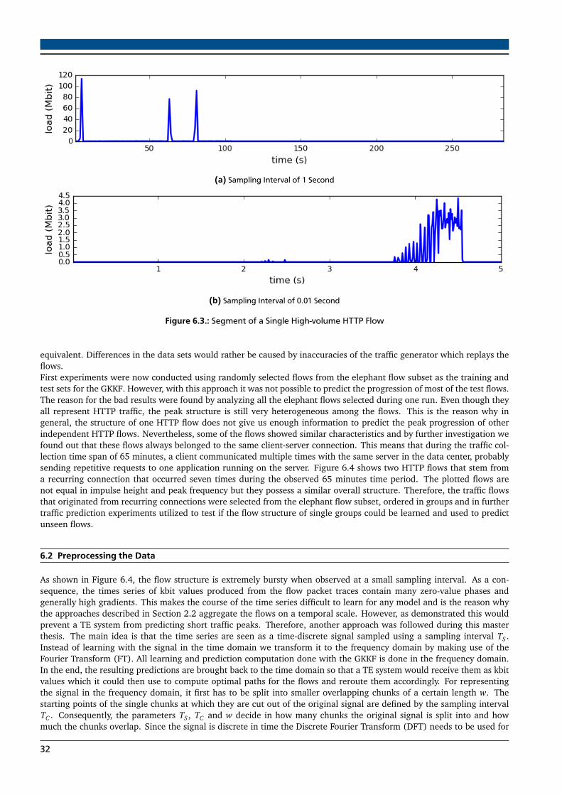
(a) Sampling Interval of 1 Second

(b) Sampling Interval of 0.01 Second

Figure 6.3.: Segment of a Single High-volume HTTP Flow

equivalent. Differences in the data sets would rather be caused by inaccuracies of the traffic generator which replays theflows.First experiments were now conducted using randomly selected flows from the elephant flow subset as the training andtest sets for the GKKF. However, with this approach it was not possible to predict the progression of most of the test flows.The reason for the bad results were found by analyzing all the elephant flows selected during one run. Even though theyall represent HTTP traffic, the peak structure is still very heterogeneous among the flows. This is the reason why ingeneral, the structure of one HTTP flow does not give us enough information to predict the peak progression of otherindependent HTTP flows. Nevertheless, some of the flows showed similar characteristics and by further investigation wefound out that these flows always belonged to the same client-server connection. This means that during the traffic col-lection time span of 65 minutes, a client communicated multiple times with the same server in the data center, probablysending repetitive requests to one application running on the server. Figure 6.4 shows two HTTP flows that stem froma recurring connection that occurred seven times during the observed 65 minutes time period. The plotted flows arenot equal in impulse height and peak frequency but they possess a similar overall structure. Therefore, the traffic flowsthat originated from recurring connections were selected from the elephant flow subset, ordered in groups and in furthertraffic prediction experiments utilized to test if the flow structure of single groups could be learned and used to predictunseen flows.

6.2 Preprocessing the Data

As shown in Figure 6.4, the flow structure is extremely bursty when observed at a small sampling interval. As a con-sequence, the times series of kbit values produced from the flow packet traces contain many zero-value phases andgenerally high gradients. This makes the course of the time series difficult to learn for any model and is the reason whythe approaches described in Section 2.2 aggregate the flows on a temporal scale. However, as demonstrated this wouldprevent a TE system from predicting short traffic peaks. Therefore, another approach was followed during this masterthesis. The main idea is that the time series are seen as a time-discrete signal sampled using a sampling interval TS .Instead of learning with the signal in the time domain we transform it to the frequency domain by making use of theFourier Transform (FT). All learning and prediction computation done with the GKKF is done in the frequency domain.In the end, the resulting predictions are brought back to the time domain so that a TE system would receive them as kbitvalues which it could then use to compute optimal paths for the flows and reroute them accordingly. For representingthe signal in the frequency domain, it first has to be split into smaller overlapping chunks of a certain length w. Thestarting points of the single chunks at which they are cut out of the original signal are defined by the sampling intervalTC . Consequently, the parameters TS , TC and w decide in how many chunks the original signal is split into and howmuch the chunks overlap. Since the signal is discrete in time the Discrete Fourier Transform (DFT) needs to be used for

32

Figure 6.4.: Traffic Flows of Recurring Client-Server Communication

the transformation and by splitting the signal in chunks, basically a discrete-time Short-Time Fourier Transform (STFT)is performed, whereas a Fast Fourier Transform (FFT) algorithm is used for making the FT computations faster.

One main advantage of learning with the traffic signal in the frequency instead of the time domain is that the datasets the GKKF has to deal with become less bursty. Figure 6.5 compares the courses of different data series. In Figure6.5a a 1 second long flow chunk is shown. When computing the FT of the chunk, a data series as shown in Figure6.5b is produced. The data series consists of complex numbers that describe the amplitudes and phases of simple sinewaves that can be combined to construct the original signal. In the plot the amplitudes of the needed sine waves areshown. Furthermore, the plot reveals that the frequency values get folded at the Nyquist frequency fN which is half ofthe sampling frequency, fN = 0.5 fS = 0.5 1

TS. For reconstructing the time signal from sine waves we therefore only need

to save the first N values of the FT results, whereas N = fN + 1. When transforming our results back to the time domain,the rest of the values can be reconstructed by inverting the imaginary parts of the saved complex numbers. However, inorder to use the FT results with the GKKF, the complex numbers have to be split into their real and imaginary parts. Theresulting data series consisting alternately of real and imaginary values is presented in Figure 6.5c which clearly showsthat the data series is considerably less bursty then the original time series.Another advantage of conducting the calculations in the frequency domain is that since the FT is built over a part of thesignal, much more information about the flow structure is contained in every data point which makes it easier to observethe current condition of the flow. Furthermore, since TC > TS the data set will contain less data points in the frequencythan in the time domain. This is especially useful when the training set consists of very long flows that would otherwiseresult in a large number of data points. The selection of an appropriate value for TC that leads to an overlap of the chunksalso reduces artifacts in the frequency domain.

The influence of the transition to the frequency domain on the employed data set should now be illustrated using anexample. We assume that the training set the GKKF should learn from consists of only one short high-volume flow witha duration of 10 seconds. When using a sampling interval TS = 0.01 our training set datat rain contains a time series ofkbit values observed at every 0.01 seconds and which possesses the dimensionality datat rain ∈ R1000x1. As mentionedbefore, the time signal is now split into single overlapping chunks. When using a sampling interval TC = 0.05 and achunk length of w = 1 the signal is split into 200 unique chunks that all contain 100 data points, whereas always 20subsequent chunks overlap. In the next step, the FT is computed which returns a data series of 100 complex numbers forevery chunk which represents a single observation in the frequency domain. As mentioned before, we only have to keepthe first N frequencies but need to split them into their real and imaginary parts which in the end leaves us with a seriesof 102 data points for every chunk. Altogether, our training set will now have the dimensionality datat rain ∈ R200x102.As we can see, the ability to work with the traffic data needs to be paid with an increase of the observation dimensionality.

As shown in [39], the GKKF is able to process data with a very high dimensionality. Nevertheless, an attempt wasmade to reduce the dimensions needed for a single observation to lower their complexity and save computation time.

33

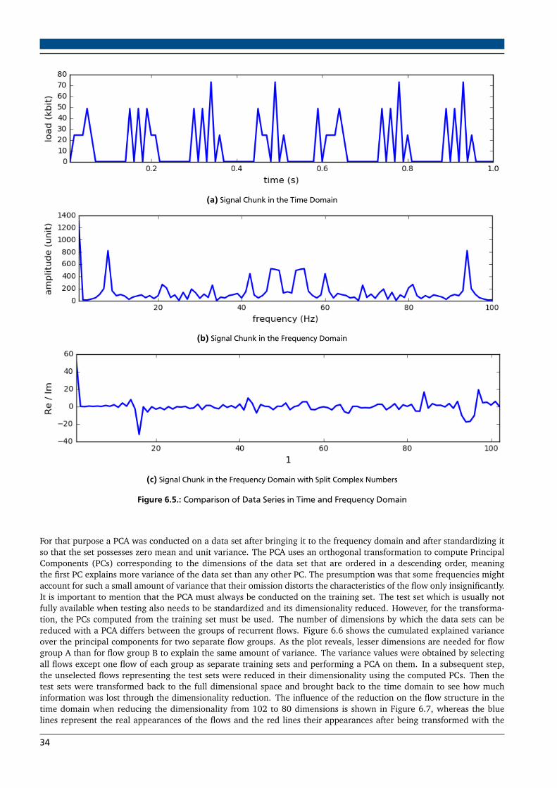
(a) Signal Chunk in the Time Domain

(b) Signal Chunk in the Frequency Domain

(c) Signal Chunk in the Frequency Domain with Split Complex Numbers

Figure 6.5.: Comparison of Data Series in Time and Frequency Domain

For that purpose a PCA was conducted on a data set after bringing it to the frequency domain and after standardizing itso that the set possesses zero mean and unit variance. The PCA uses an orthogonal transformation to compute PrincipalComponents (PCs) corresponding to the dimensions of the data set that are ordered in a descending order, meaningthe first PC explains more variance of the data set than any other PC. The presumption was that some frequencies mightaccount for such a small amount of variance that their omission distorts the characteristics of the flow only insignificantly.It is important to mention that the PCA must always be conducted on the training set. The test set which is usually notfully available when testing also needs to be standardized and its dimensionality reduced. However, for the transforma-tion, the PCs computed from the training set must be used. The number of dimensions by which the data sets can bereduced with a PCA differs between the groups of recurrent flows. Figure 6.6 shows the cumulated explained varianceover the principal components for two separate flow groups. As the plot reveals, lesser dimensions are needed for flowgroup A than for flow group B to explain the same amount of variance. The variance values were obtained by selectingall flows except one flow of each group as separate training sets and performing a PCA on them. In a subsequent step,the unselected flows representing the test sets were reduced in their dimensionality using the computed PCs. Then thetest sets were transformed back to the full dimensional space and brought back to the time domain to see how muchinformation was lost through the dimensionality reduction. The influence of the reduction on the flow structure in thetime domain when reducing the dimensionality from 102 to 80 dimensions is shown in Figure 6.7, whereas the bluelines represent the real appearances of the flows and the red lines their appearances after being transformed with the

34

Figure 6.6.: Cumulative Explained Variance per Dimension

PCs. For flow group A, a reduction of 20 dimensions leaves us with 97.4% of explained variance. The loss of informationis still acceptable, even though it is clearly visible in the plot. For flow group B, the remaining 80 dimensions are stillenough to explain 93.3% of the variance. However, the plot demonstrates that for this flow group a larger percentage ofinformation was contained in the omitted 20 dimensions since the heights of the flow peaks differ more from the originalones. Therefore, the results match the insights already obtained from Figure 6.6. Considering also the results for otherflow groups, it has to be concluded that a PCA is only useful to a limited extend for reducing the dimensionality of theutilized traffic data since a reduction of only around 20 dimensions could be achieved in the best cases.

As mentioned before, the training sets used during the experiments contain observations of kbit values which werecalculated from the flows’ .pcap files. The kbit values the flows reach on the network are influenced by the applicationsrunning on the communicating hosts that produce the flows. Furthermore, their courses also depend on network ele-ments like the network switches that forward the traffic or the links between them. All these components together forman underlying process or system, whereas the resulting kbit values of a single flow can be seen as observations emittedby the system. However, these observations do not represent the true state of the underlying process since differentsituations in the network defined by the condition of the flow-producing applications, switches, links or the appearanceof other traffic, could produce the same kbit observations for the regarded flow. The true very complex state of theprocess is therefore hidden which is why the powerful concept of HMMs was used during this master thesis for modelingthe process. Our training sets only contain the mentioned observations, however, as noted in Section 4.4, a windowof observations can be used as an internal state representation. By computing the FT over chunks of the signal we areactually already building a window because the state is represented by the frequencies of a time signal chunk that con-sists of multiple observations. However, to extend the representation of the state during the prediction experiments, itwas formed using the FTs of multiple chunks with increasing length. One possibility would e.g. be to use the FT of thenext second and combine it with the FTs computed over the next 2 and 3 seconds. This allows us to include some morelong-term behavior of the flow in the state representation. In such a scenario, an observation would be represented bythe FT over the next second of the time signal.

6.3 Experimental Results

As mentioned before, the elephant flows were grouped by flows that stemmed from recurrent socket-to-socket connec-tions. For the prediction experiments, the 20 groups with the highest numbers of flows were selected. The experimentresults are shown in Table 6.1, whereas the column # of flows holds the information about how many flows each groupcontained. On average, one group consisted of 8 unique flows. The performance of the GKKF was tested on every flowgroup separately. During an experiment, always one flow was selected as the test set. The rest of the flows were used forconstructing the training set. As noted in previous sections, the data set representing a flow consists of a time series ofkbit values, whereas for the prediction experiments described in this section, a sampling interval TS = 0.01 was used forproducing the data series and a chunk sampling interval of TC = 0.05 for splitting them into smaller chunks.In Section 6.1 we showed the results of our traffic data analysis which revealed that HTTP traffic flows often consist ofshort traffic peaks that in turn can be divided in a rising phase and a phase with a mainly constant load level. Bensonet al. [16] already demonstrated that a certain percentage of the overall traffic in a data center remains constant over ashort period of time, meaning that the traffic load does not fluctuate by more than 20%. In such a scenario, the meancomputed over the last short time period can be used for estimating the load of the flow in the next period. For this

35

(a) Test Flow from Flow Group A

(b) Test Flow from Flow Group B

Figure 6.7.: Influence of Dimensionality Reduction on the Flow Appearance

reason, the authors define such a traffic flow as predictable. However, at the time point from which on the flow loadremains constant, congestion might already have happened in the network. Therefore, the more important parts of theflows are the peak rises, which is why we explicitly concentrate our predictions on these parts. We tested the ability ofthe GKKF to predict the peak rises after providing it with only a few observations from the beginning of the peak. Thenumber of observations differs between the flows and ranges between 3 and 60 steps in the frequency domain whichcorresponds to an observed time interval of 0.15 to 3 seconds. When the observation stops and the true prediction begins,all flows still possess a low traffic load which then increases rapidly by around 150% on average during the next second.Therefore, when utilizing the definition from [16] all used traffic flows would need to be considered as unpredictable atthe point of the last observation.The GKKF was always used for predicting a time period of 1 second, resulting in 20 prediction steps in the frequency do-main. The highest single impulse value predicted by the GKKF during this period was then compared to the true highestimpulse value in the same period. The difference between both values divided by the true highest value represents theapplied error metric for the prediction. The error should always be compared to the information that was already givenin the observations. Therefore, another error metric was calculated for every flow group which helps to assess the qualityof the prediction. In Table 6.1 the metric is shown in the constant error column. It was calculated like the predictionerror only that the highest impulse value which emerged during the observation phase was used as the prediction, just asif we would predict a constant load. Since we only observe the beginning of the peak rise, the picked impulse value willalways be smaller than the true one during the next second. Consequently, the true value will always be underestimatedwhich is why all values in the column are negative.

During the first set of experiments a chunk length w = 1 was used for all flow groups. The internal state represen-tation was then built by combining the FTs of the next second, the next 2 seconds and the next 3 seconds of the signal.An observation was represented by the FT of the next second. The prediction errors obtained for all flow groups areshown in column chunk len. = 1 s. The performance of the GKKF for predicting a particular flow group is indicatedby a red, yellow or green coloring of the associated table cell which corresponds to a bad, moderate or good predictionperformance. Since it is difficult to assess the true prediction quality solely based on error metrics, a two-step approachwas used.In the first step, the computed prediction error and constant error values were utilized. Whenever the prediction errorwas above 50% or equally bad as the corresponding constant error value, the quality of the prediction was considered in-sufficient and the flow group marked in red. When the prediction error was lower than 50% and clearly smaller than theconstant error, the group was marked in yellow. Only if a prediction error of less than 20% was achieved, the predictionwas classified as good and marked in green. Subsequently, as a second step, a manual verification of the prediction was

36

prediction error

group ID # flows constant error optimal chunk len. chunk len. = 1 s chunk len. = optimal

1 4 -69.7% 0.15 s -43.1% -2.0%

2 13 -60.1% 0.4 s -36.3% -8.4%

3 6 -63.5% 0.55 s 14.7% 5.6%

4 24 -57.6% 0.2 s -62.3% -22.8%

5 5 -55.9% 0.2 s -53.1% -12.1%

6 6 -46.9% 0.15 s -52.8% -13.2%

7 3 -60.0% 0.25 s -4.5% 2.5%

8 10 -79.6% 0.3 s -28.5% -4.3%

9 4 -66.7% 1.95 s -28.4% -4.1%

10 4 -63.2% 0.5 s -46.7% -0.7%

11 5 -54.3% 0.25 s -26.8% -0.8%

12 18 -60.4% 0.95 s -44.2% -10.2%

13 5 -45.5% 0.55 s -11.6% -1.6%

14 3 -62.5% 0.35 s -63.8% -10.2%

15 11 -52.2% 0.25 s -57.9% -17.0%

16 13 -37.5% 0.55 s -70.6% -40.2%

17 3 -26.4% 0.95 s -93.2% -45.4%

18 4 -35.7% 0.45 s 151.9% 4.7%

19 7 -70.0% 0.15 s -53.5% -7.3%

20 3 -62.5% 0.95 s -53.7% 2.0%

Table 6.1.: Prediction Experiments Results

done by comparing the predicted time series with its true counterpart. Only if the group dependent overall peak structurewas visible in the predicted time series, the prediction of a flow group could retain its classification as moderate or good.If the prediction did not show the key characteristics found in the flows that made up the training set, the predictionquality got downgraded and the group marked in red.When evaluating the prediction results for all groups using the described procedure, only a bad prediction performancewas achieved for 11 out of 20 groups. A moderate prediction performance was obtained for 6 groups and a good onefor 3 groups. To illustrate the differences between the performance classes, examples are shown in Figure 6.8. The plotsalways compare the predicted flow signal in the time domain to the true appearance of the flow, whereas the predictioncorresponds to the mean prediction values obtained from the GKKF. The prediction variances were omitted in order toproduce clearer plots. Figure 6.8a shows the prediction for flow group 3 which was classified as achieving a good perfor-mance. As clearly visible in the plot, the predicted flow has the same structure as the ground truth, even after time point0.5 s from which on no further observations were obtained. The value of the highest impulse is slightly overestimated,resulting in a positive error prediction value of 14.7%. The results for flow group 19, shown in Figure 6.8b, again showmatching flow structures for the predicted and true time series. However, this time, the predicted highest impulse valueis further away from the true value which results in a prediction error of more than 50% and therefore, the group ismarked in red. In Figure 6.8c we can see that for flow group 18 the highest impulse value is overestimated to a largedegree. Furthermore, the predicted peak structure shows clear differences to the true appearance of the peak which iswhy classifying the prediction quality as bad is inevitable.

As mentioned, a chunk length of w = 1 was used so far for every flow group. However, the selected value mightnot be optimal for learning and predicting the peak structure of every flow group. When the test flow differs considerably

37

(a) Flow Group 3: Observations were obtained until time point 0.5 s

(b) Flow Group 19: Observations were obtained until time point 0.8 s

(c) Flow Group 18: Observations were obtained until time point 0.5 s

Figure 6.8.: Prediction Results with Chunk Length 1 Second

from the training flows in a very small part of the signal, it might be beneficial to use a smaller chunk length so that thisunique part will be included into fewer chunks and therefore fewer observations. The assumption was verified by findingthe optimal chunk length for every flow group, whereas values between 0.1 and 1.95 seconds for w were tested. Theresults are shown in column optimal chunk len.. The associated prediction errors achieved when utilizing these lengthsare given in column chunk len. = optimal. By solely looking at the resulting error values the prediction quality seemedto improve for all flow groups. However, the low error values achieved for a specific chunk length could also just be acoincidence, meaning that the actual performance quality is bad but the highest predicted impulse is nevertheless closeto the true value. For evaluating if a chunk length really improves the prediction, the error values achieved for all testedchunk lengths need to be analyzed. In Figure 6.9, the error values are shown for the flow groups 19 and 18. As wecan see for flow group 19 in Figure 6.9a, the initially selected chunk length of 1 second was too long which is why aprediction error of more then 50% was achieved and the prediction performance therefore classified as bad. However, nomatter which chunk length was selected, the highest impulse was always predicted with an error of not more then 63.8%.Furthermore, the error values do not oscillate. This indicates that the peak structure can be predicted in general and thehighest impulse in particular when the optimal chunk length is selected. A different situation is observed for flow group18. Even though the prediction error is low for the best chunk length, Figure 6.9b shows that the error values oscillate toa high degree in the area from 0.1 to 1 second. Moreover, when using a higher chunk length, no prediction error valuebelow 100% can be achieved which leads to the conclusion that the peak structure cannot be correctly predicted.For evaluating the prediction performance the described two-step approach was used again. Additionally, in a third step,the information obtained from plots similar to those in Figure 6.9 were utilized to possibly downgrade the performancelevel, marking the flow group in red. After the classification process, a good performance quality could be validated for14 out of 20 groups. By selecting a better chunk length, the prediction of all flow groups that were earlier marked in

38

(a) Flow Group 19 (b) Flow Group 18

Figure 6.9.: Chunk Length Dependent Prediction Errors

yellow or green could be improved. The reason is that for these groups, a correct prediction of the peaks’ key character-istics could already be achieved when using a chunk length of 1 second. The same applies to the flow groups 5, 6, 14, 15and 19 which were only marked in red because the error values exceeded the 50% mark. The prediction improvementsachieved for flow group 19 are shown in Figure 6.10a. The key characteristics of the peak structure still get predictedand furthermore, the predicted highest impulse is closer to the true highest value. The fact that the highest impulse ispredicted at a different time point is caused by the differences between the training and test flows.For the remaining groups 4, 9, 16, 17, 18 and 20, only a bad performance could be achieved. Even though all flowsforming one group stemmed from the same recurring socket-to-socket connection, the similarities between them was notstrong enough so that the GKKF could learn the key characteristics from the training flows and use them to correctlypredict the peak structure in the test flows. The prediction results for flow group 18, when using the optimized chunklength, are shown in Figure 6.10b. Despite predicting the true highest impulse value, the structure of the predicted timeseries is clearly different to the true one.

(a) Flow Group 19: Observations were obtained until time point 0.8 s

(b) Flow Group 18: Observations were obtained until time point 0.5 s

Figure 6.10.: Prediction Results with Optimized Chunk Length

39

7 ConclusionDuring this master thesis, a framework was developed which allows the user to set up a scalable virtualized SDN with acustom topology and perform experiments with it. In one implemented type of experiment, statistical information wascollected from the network devices and processed by the SDN controller to form observations that were planned to beused for the traffic prediction experiments. However, the analysis of real data center traffic revealed that a very smallobservation sampling interval would be needed, which cannot be produced with the currently implemented approach.Further development of the experiment framework should therefore focus on delegating some of the processing stepsto the network devices, since observations could then be produced at a much higher sampling frequency. This could beachieved by extending the existing OVS implementation as shown in [79].Performing the data processing partially decentralized at the network devices should also be considered in the devel-opment of any prospective TE system that aims at predicting and rerouting network traffic in SDNs. In such a system,network devices could use their own statistical information to identify elephant flows and produce observation setswhich could then be fed into machine learning methods like the GKKF that would run locally on the devices and copewith the learning and prediction problem. The prediction results would then be sent to the controller and since thiswould only be done for elephant flows, the amount of produced control traffic would be drastically reduced. Further-more, by splitting the prediction problem among the network devices, each instance of the utilized machine learningalgorithm would have to deal with a smaller number of flows than one central algorithm. In a subsequent step, thecentral controller could form a global view of the current network situation from the received predictions and com-pute optimal paths for the dedicated flows, e.g. by formulating the goal of network throughput maximization as amulti-commodity flow problem, as shown by Agarwal et al. [11]. As a last step, the controller would then implementthe optimal paths in the network in order to alter its routing behavior, thereby preventing upcoming congestion situations.

The approach used during this master thesis for predicting traffic flows focused on the small time scale prediction ofpeak structures of single flows because, as shown during the analysis of real network traffic, this is the only type ofprediction that truly considers the existing bursty nature of the network traffic that is one important cause of networkcongestion. In the conducted traffic prediction experiments, the GKKF was used to predict the peak rises in flow groupsconsisting of single flows from recurrent socket-to-socket connections, whereas observations were only given to the GKKFwhilst the flows’ traffic load was still low. In 70% of the observed groups, a prediction of the highest traffic impulse duringthe next second could be achieved with an error of less then 20%. However, some constraints of these results need to bementioned.Firstly, a correctly predicted highest impulse value only states that no higher kbit value will be reached during a timeinterval of 10 ms in the next second. It does not directly tell us how high the overall load of the flow will be during thistime span. However, when analyzing the peak structure of flows it can be observed that the impulses themselves oftenappear at a constant frequency depending on the associated flow group. Therefore, the total load produced during thenext second could be estimated by deriving the impulse frequency from the observation phase and combining in with theprediction of the highest impulse value. Future work could evaluate, if it is possible to achieve a reasonable estimationof the total flow volume with this approach.Secondly, the predicted flows were closely related since they stemmed from recurrent socket-to-socket connections. All ofthe flows occurred during a time span of only 65 minutes. Further research could now try to evaluate, if the similaritiesare also persistent over a longer period of time which would give hints at which frequency the model of the underlyingsystem would have to be relearned. The observation of longer time periods could also reveal that the prediction of acertain flow group gets easier when more unique flow instances of one group are collected. Moreover, further researchshould assess, if recurrent flows make up a share of the total network traffic that is big enough so that a TE systemutilizing the predictions could influence an adequate amount of the overall network traffic.Thirdly, during this master thesis, the different flow groups were learned and tested independently to see, if the peakstructures could generally be learned and predicted. However in practice, a TE system would need to handle a largenumber of flows which is why all or multiple flow groups probably would need to be combined to larger training sets sothat only one or a few different models would have to be learned. Therefore, future research on the feasibility of a TEsystem capable of traffic prediction would need to investigate, if a prediction is still possible in such a scenario using theproposed approach.

40

Bibliography[1] “Software-defined networking: The new norm for networks (white paper).” https://www.opennetworking.org/images/stories/downloads/sdn-resources/white-papers/wp-sdn-newnorm.pdf, 2012. [Online; accessed 23-Sept.-2016].

[2] A. Botta, W. de Donato, A. Dainotti, S. Avallone, and A. Pescapé, “D-itg 2.8.1 manual.” http://traffic.comics.unina.it/software/ITG/manual/, 2013. [Online; accessed 23-Sept.-2016].

[3] B. Pfaff, J. Pettit, T. Koponen, E. J. Jackson, A. Zhou, J. Rajahalme, J. Gross, A. Wang, J. Stringer, P. Shelar,K. Amidon, and M. Casado, “The design and implementation of open vswitch,” in Proceedings of the 12th USENIXConference on Networked Systems Design and Implementation, NSDI’15, pp. 117–130, 2015.

[4] B. Lantz, B. Heller, and N. McKeown, “A network in a laptop: Rapid prototyping for software-defined networks,” inProceedings of the 9th ACM SIGCOMM Workshop on Hot Topics in Networks, Hotnets-IX, pp. 19:1–19:6, 2010.

[5] P. Wette, M. Dräxler, and A. Schwabe, “Maxinet: Distributed emulation of software-defined networks,” in NetworkingConference, 2014 IFIP, pp. 1–9, 2014.

[6] T. Benson, A. Anand, A. Akella, and M. Zhang, “Understanding data center traffic characteristics,” SIGCOMM Com-put. Commun. Rev., vol. 40, pp. 92–99, 2010.

[7] M. Chiesa, G. Kindler, and M. Schapira, “Traffic engineering with equal-cost-multipath: An algorithmic perspective,”in IEEE INFOCOM 2014 - IEEE Conference on Computer Communications, pp. 1590–1598, 2014.

[8] Z. Shu, J. Wan, J. Lin, S. Wang, D. Li, S. Rho, and C. Yang, “Traffic engineering in software-defined networking:Measurement and management,” IEEE Access, vol. 4, pp. 3246–3256, 2016.

[9] S. Jain, A. Kumar, S. Mandal, J. Ong, L. Poutievski, A. Singh, S. Venkata, J. Wanderer, J. Zhou, M. Zhu, J. Zolla,U. Hölzle, S. Stuart, and A. Vahdat, “B4: Experience with a globally-deployed software defined wan,” in Proceedingsof the ACM SIGCOMM 2013 Conference on SIGCOMM, SIGCOMM ’13, pp. 3–14, 2013.

[10] C. Hong, S. Kandula, R. Mahajan, M. Zhang, V. Gill, M. Nanduri, and R. Wattenhofer, “Achieving high utilizationwith software-driven wan,” in Proceedings of the ACM SIGCOMM 2013 Conference on SIGCOMM, SIGCOMM ’13,pp. 15–26, 2013.

[11] S. Agarwal, M. Kodialam, and T. V. Lakshman, “Traffic engineering in software defined networks,” in INFOCOM,2013 Proceedings IEEE, pp. 2211–2219, 2013.

[12] M. Al-Fares, S. Radhakrishnan, B. Raghavan, N. Huang, and A. Vahdat, “Hedera: Dynamic flow scheduling for datacenter networks,” in Proceedings of the 7th USENIX Conference on Networked Systems Design and Implementation,NSDI’10, pp. 19–19, 2010.

[13] A. R. Curtis, W. Kim, and P. Yalagandula, “Mahout: Low-overhead datacenter traffic management using end-host-based elephant detection,” in INFOCOM, 2011 Proceedings IEEE, pp. 1629–1637, 2011.

[14] A. R. Curtis, J. C. Mogul, J. Tourrilhes, P. Yalagandula, P. Sharma, and S. Banerjee, “Devoflow: Scaling flow man-agement for high-performance networks,” in Proceedings of the ACM SIGCOMM 2011 Conference, SIGCOMM ’11,pp. 254–265, 2011.

[15] F. François and E. Gelenbe, “Towards a cognitive routing engine for software defined networks,” CoRR,vol. abs/1602.00487, 2016.

[16] T. Benson, A. Anand, A. Akella, and M. Zhang, “Microte: Fine grained traffic engineering for data centers,” inProceedings of the Seventh COnference on Emerging Networking EXperiments and Technologies, CoNEXT ’11, pp. 8:1–8:12, 2011.

[17] P. K. Hoong, I. K. T. Tan, and C. Y. Keong, “Bittorrent network traffic forecasting with ARMA,” CoRR,vol. abs/1208.1896, 2012.

41

[18] N. K. Hoong, P. K. Hoong, I. K. T. Tan, N. Muthuvelu, and L. C. Seng, “Impact of utilizing forecasted networktraffic for data transfers,” in Advanced Communication Technology (ICACT), 2011 13th International Conference on,pp. 1199–1204, 2011.

[19] Y. Yu, M. Song, Y. Fu, and J. Song, “Traffic prediction in 3g mobile networks based on multifractal exploration,”Tsinghua Science and Technology, vol. 18, no. 4, pp. 398–405, 2013.

[20] B. Vujicic, H. Chen, and L. Trajkovic, “Prediction of traffic in a public safety network,” in 2006 IEEE InternationalSymposium on Circuits and Systems, pp. 4 pp.–, 2006.

[21] N. C. Anand, C. Scoglio, and B. Natarajan, “Garch - non-linear time series model for traffic modeling and predic-tion,” in NOMS 2008 - 2008 IEEE Network Operations and Management Symposium, pp. 694–697, 2008.

[22] D. C. Park and D. M. Woo, “Prediction of network traffic using dynamic bilinear recurrent neural network,” in 2009Fifth International Conference on Natural Computation, vol. 2, pp. 419–423, 2009.

[23] S. Chabaa, A. Zeroual, and J. Antari, “Identification and prediction of internet traffic using artificial neural net-works,” Intelligent Learning Systems and Applications, vol. 2, no. 3, pp. 147–155, 2010.

[24] P. Cortez, M. Rio, M. Rocha, and P. Sousa, “Internet traffic forecasting using neural networks,” in The 2006 IEEEInternational Joint Conference on Neural Network Proceedings, pp. 2635–2642, 2006.

[25] Y. Chen, B. Yang, and Q. Meng, “Small-time scale network traffic prediction based on flexible neural tree,” AppliedSoft Computing, vol. 12, no. 1, pp. 274 – 279, 2012.

[26] C. N. Babu and B. E. Reddy, “Performance comparison of four new arima-ann prediction models on internet trafficdata,” Journal of Telecommunications and Information Technology, pp. 67–75, 2015.

[27] S. Chabaa, A. Zeroual, and J. Antari, “Anfis method for forecasting internet traffic time series,” in 2009 Mediterran-nean Microwave Symposium (MMS), pp. 1–4, 2009.

[28] Y. Liang and L. Qiu, “Network traffic prediction based on svr improved by chaos theory and ant colony optimization,”International Journal of Future Generation Communication and Networking, vol. 8, no. 1, pp. 69–78, 2015.

[29] R. E. Kalman, “A new approach to linear filtering and prediction problems,” Transactions of the ASME–Journal ofBasic Engineering, vol. 82, no. Series D, pp. 35–45, 1960.

[30] B. A. McElhoe, “An assessment of the navigation and course corrections for a manned flyby of mars or venus,” IEEETransactions on Aerospace and Electronic Systems, vol. AES-2, no. 4, pp. 613–623, 1966.

[31] E. A. Wan and R. V. D. Merwe, “The unscented kalman filter for nonlinear estimation,” in Adaptive Systems for SignalProcessing, Communications, and Control Symposium 2000. AS-SPCC. The IEEE 2000, pp. 153–158, 2000.

[32] D. J. Hsu, S. M. Kakade, and T. Zhang, “A spectral algorithm for learning hidden markov models,” CoRR,vol. abs/0811.4413, 2008.

[33] H. Jaeger, “Observable operator models for discrete stochastic time series,” Neural Comput., vol. 12, no. 6, pp. 1371–1398, 2000.

[34] S. Vempala and G. Wang, “A spectral algorithm for learning mixture models,” J. Comput. Syst. Sci., vol. 68, no. 4,pp. 841–860, 2004.

[35] L. Song, B. Boots, S. M. Siddiqi, G. J. Gordon, and A. J. Smola, “Hilbert space embeddings of hidden markovmodels,” in Proceedings of the 27th International Conference on Machine Learning (ICML-10), pp. 991–998, 2010.

[36] G. Gebhardt, “Embedding kalman filters into reproducing kernel hilbert spaces,” 2014.

[37] L. Ralaivola and F. d’Alche Buc, “Time series filtering, smoothing and learning using the kernel kalman filter,” inProceedings. 2005 IEEE International Joint Conference on Neural Networks, 2005., vol. 3, pp. 1449–1454, 2005.

[38] P. Zhu, B. Chen, and J. C. Prı´ncipe, “Learning nonlinear generative models of time series with a kalman filter inrkhs,” IEEE Transactions on Signal Processing, vol. 62, no. 1, pp. 141–155, 2014.

[39] G. Gebhardt and G. Neumann, “The generalized kernel kalman filter - learning forward models from high-dimensional partial observations (internal report),” 2015.

42

[40] https://www.opennetworking.org/index.php. [Online; accessed 23-Sept.-2016].

[41] “Openflow switch specification version 1.5.1.” https://www.opennetworking.org/images/stories/downloads/sdn-resources/onf-specifications/openflow/openflow-switch-v1.5.1.pdf, 2015. [Online; accessed 23-Sept.-2016].

[42] “The benefits of multiple flow tables and ttps.” https://www.opennetworking.org/images/stories/downloads/sdn-resources/technical-reports/TR_Multiple_Flow_Tables_and_TTPs.pdf, 2015. [Online; accessed 23-Sept.-2016].

[43] A. Krogh, M. Brown, I. S. Mian, K. Sjölander, and D. Hausder, “Hidden markov models in computational biologyapplications to protein modeling,” Journal of molecular biology, vol. 235, no. 5, pp. 1501–1531, 1994.

[44] M. Gales and S. Young, “The application of hidden markov models in speech recognition,” Foundations and Trendsin Signal Processing, vol. 1, no. 3, pp. 195–304, 2007.

[45] A. D. Wilson and A. F. Bobick, “Parametric hidden markov models for gesture recognition,” IEEE Transactions onPattern Analysis and Machine Intelligence, vol. 21, no. 9, pp. 884–900, 1999.

[46] C. Kohlschein, “An introduction to hidden markov models.” http://www.tcs.rwth-aachen.de/lehre/PRICS/WS2006/kohlschein.pdf, 2006. [Online; accessed 23-Sept.-2016].

[47] Z. Ghahramani, “An introduction to hidden markov models and bayesian networks,” International Journal of PatternRecognition and Artificial Intelligence, vol. 15, no. 1, pp. 9–42, 2001.

[48] J. A. Bilmes, “A gentle tutorial of the em algorithm and its application to parameter estimation for gaussian mix-ture and hidden markov models.” http://melodi.ee.washington.edu/people/bilmes/mypapers/em.pdf, 1998.[Online; accessed 23-Sept.-2016].

[49] C. Cortes and V. Vapnik, “Support-vector networks,” Mach. Learn., vol. 20, no. 3, pp. 273–297, 1995.

[50] C. E. Rasmussen and C. K. I. Williams, Gaussian Processes for Machine Learning (Adaptive Computation and MachineLearning). The MIT Press, 2005.

[51] L. Wehbe, “Kernel properties - convexity.” http://alex.smola.org/teaching/cmu2013-10-701x/slides/recitation_3_kernel_properties_convexity.pdf, 2013. [Online; accessed 23-Sept.-2016].

[52] N. Aronszajn, “Theory of reproducing kernels,” Transactions of the American Mathematical Society, vol. 68, no. 3,pp. 337–404, 1950.

[53] A. Smola, A. Gretton, L. Song, and B. Schölkopf, “A hilbert space embedding for distributions,” in Proceedings of the18th International Conference on Algorithmic Learning Theory, ALT ’07, pp. 13–31, 2007.

[54] L. Song, K. Fukumizu, and A. Gretton, “Kernel embeddings of conditional distributions: A unified kernel frameworkfor nonparametric inference in graphical models,” IEEE Signal Processing Magazine, vol. 30, no. 4, pp. 98–111, 2013.

[55] G. Gebhardt, A. Kupcsik, and G. Neumann, “Learning subspace conditional embedding operators (internal report),”2015.

[56] M. Shannon, H. Zen, and W. Byrne, “Autoregressive models for statistical parametric speech synthesis,” IEEE Trans-actions on Audio, Speech, and Language Processing, vol. 21, no. 3, pp. 587–597, 2013.

[57] W. Feng, A. Goel, A. Bezzaz, W. Feng, and J. Walpole, “Tcpivo: A high-performance packet replay engine,” in Proceed-ings of the ACM SIGCOMM Workshop on Models, Methods and Tools for Reproducible Network Research, MoMeTools’03, pp. 57–64, 2003.

[58] “Tcpreplay.” http://tcpreplay.synfin.net/. [Online; accessed 23-Sept.-2016].

[59] S. Hong and S. F. Wu, “On interactive internet traffic replay,” in Recent Advances in Intrusion Detection: 8th Interna-tional Symposium, RAID 2005, pp. 247–264, 2006.

[60] A. Botta, A. Dainotti, and A. Pescapé, “A tool for the generation of realistic network workload for emerging net-working scenarios,” Comput. Netw., vol. 56, no. 15, pp. 3531–3547, 2012.

43

[61] “Kernel virtual machine.” http://www.linux-kvm.org/. [Online; accessed 23-Sept.-2016].

[62] “Xen project.” https://www.xenproject.org. [Online; accessed 23-Sept.-2016].

[63] “Virtual box.” https://www.virtualbox.org/. [Online; accessed 23-Sept.-2016].

[64] “Using open vswitch without kernel support.” https://github.com/openvswitch/ovs/blob/master/INSTALL.userspace.md. [Online; accessed 23-Sept.-2016].

[65] “Estinet.” http://www.estinet.com/. [Online; accessed 23-Sept.-2016].

[66] “ns-3.” https://www.nsnam.org/. [Online; accessed 23-Sept.-2016].

[67] “Omnet++.” https://omnetpp.org/. [Online; accessed 23-Sept.-2016].

[68] “Ryu.” https://osrg.github.io/ryu/. [Online; accessed 23-Sept.-2016].

[69] “Pox.” https://github.com/noxrepo/pox. [Online; accessed 23-Sept.-2016].

[70] “Project floodlight.” http://www.projectfloodlight.org/floodlight/. [Online; accessed 23-Sept.-2016].

[71] G.Karypis and V. Kumar, “Unstructured graph partitioning and sparse matrix ordering system version 2.0 (technicalreport).” http://citeseerx.ist.psu.edu/viewdoc/download?doi=10.1.1.38.376&rep=rep1&type=pdf, 1995.[Online; accessed 23-Sept.-2016].

[72] D. Schwerdel, D. Hock, D. Günther, B. Reuther, P. Müller, and P. Tran-Gia, “Tomato - a network experimentationtool,” 7th International ICST Conference on Testbeds and Research Infrastructures for the Development of Networks andCommunities (TridentCom 2011), 2011.

[73] “Openvz.” https://openvz.org/. [Online; accessed 23-Sept.-2016].

[74] M. Al-Fares, A. Loukissas, and A. Vahdat, “A scalable, commodity data center network architecture,” in Proceedingsof the ACM SIGCOMM 2008 Conference on Data Communication, SIGCOMM ’08, pp. 63–74, 2008.

[75] D. Gupta, K. Yocum, M. McNett, A. C. Snoeren, A. Vahdat, and G. M. Voelker, “To infinity and beyond: Time warpednetwork emulation,” in Proceedings of the Twentieth ACM Symposium on Operating Systems Principles, SOSP ’05,pp. 1–2, 2005.

[76] T. Benson, A. Akella, and D. A. Maltz, “Network traffic characteristics of data centers in the wild,” in Proceedings ofthe 10th ACM SIGCOMM Conference on Internet Measurement, IMC ’10, pp. 267–280, 2010.

[77] “Data set for imc 2010 data center measurement.” http://pages.cs.wisc.edu/~tbenson/IMC10_Data.html.[Online; accessed 23-Sept.-2016].

[78] “Terminal-based wireshark.” https://www.wireshark.org/docs/man-pages/tshark.html. [Online; accessed 23-Sept.-2016].

[79] P. Gorja and R. Kurapati, “Extending open vswitch to l4-l7 service aware openflow switch,” in Advance ComputingConference (IACC), 2014 IEEE International, pp. 343–347, 2014.

[80] K. B. Petersen and M. S. Pedersen, “The matrix cookbook.” https://www.math.uwaterloo.ca/~hwolkowi/matrixcookbook.pdf, 2012. [Online; accessed 23-Sept.-2016].

44

A Appendix

A.1 List of Counters in OpenFlow Version 1.5.1

45

A.2 Derivation of a Finite-dimensional Kalman Gain Matrix in Hilbert Space

Qt = Σ−ϕt

C Tφ|ϕ (Cφ|ϕΣ

−ϕt

C Tφ|ϕ + κI)−1 (A.1)

= Υ x ′ S−t Υ

Tx ′

Φy (Kx x +λOIm)−1 Υ T

x

T

Φy (Kx x +λOIm)−1 Υ T

x Υ x ′ S−t Υ

Tx ′

Φy (Kx x +λOIm)−1 Υ T

x

T+ κI

−1(A.2)

= Υ x ′ S−t Υ

Tx ′ Υ x (Kx x +λOIm)

−1ΦTy

Φy (Kx x +λOIm)−1 Kx x ′ S

−t Υ

Tx ′ Υ x (Kx x +λOIm)

−1ΦTy + κI

−1(A.3)

= Υ x ′ S−t

(Kx x +λOIm)−1Υ T

x Υ x ′TΦT

y

Φy (Kx x +λOIm)−1 Kx x ′ S

−t

(Kx x +λOIm)−1Υ T

x Υ x ′TΦT

y + κI−1

(A.4)

= Υ x ′ S−t

(Kx x +λOIm)−1Kx x ′

TΦT

y

Φy (Kx x +λOIm)−1 Kx x ′ S

−t

(Kx x +λOIm)−1Kx x ′

TΦT

y + κI−1

(A.5)

= Υ x ′ S−t OT ΦT

y︸︷︷︸

A

(Φy OS−t OT

︸ ︷︷ ︸

B

ΦTy

︸︷︷︸

A

+κI)−1, (A.6)

whereas O = (Kx x + λOIm)−1 Kx x ′ . In the next step, the matrix identity A (BA+ I)−1 = (AB+ I)−1A from [80] is appliedand we arrive at

Qt = Υ x ′ S−t OT (ΦT

y Φy OS−t OT +κIm)−1ΦT

y (A.7)

= Υ x ′ S−t OT (Gy y OS−t OT +κIm)

−1ΦTy (A.8)

= Υ x ′ Qt ΦTy , (A.9)

whereas Qt = S−t OT (GOS−t OT + κIm)−1 is the finite-dimensional Kalman gain matrix in Hilbert space and Gy y = ΦTy Φy

the Gram matrix of the embedded observations which forms the observation model matrix GO together with O.

A.3 Derivation of a Finite-dimensional Sub-space Kalman Gain Matrix in Hilbert Space

QSt = Σ

−ϕt

CSTφ|ϕ (C

Sφ|ϕΣ

−ϕt

CSTφ|ϕ +κI)−1 (A.10)

= Σ−ϕt(Φy Kx x LS

O ΓTx )

T

Φy Kx x LSO Γ

Tx Σ−ϕt(Φy Kx x LS

O ΓTx )

T + κI−1

(A.11)

= Σ−ϕtΓ x LS

O KT

x x ΦTy

︸ ︷︷ ︸

A

(Φy Kx x LSO Γ

Tx Σ−ϕtΓ x LS

O︸ ︷︷ ︸

B

KT

x x ΦTy

︸ ︷︷ ︸

A

+κI)−1, (A.12)

whereas LSO = (K

T

x x Kx x + λOIn)−1. In the next step, the matrix identity A (BA+ I)−1 = (AB+ I)−1A from [80] is appliedand we arrive at

QSt = Σ

−ϕtΓ x LS

O (KT

x x ΦTy Φy Kx x LS

O ΓTx Σ−ϕtΓ x LS

O +κIn)−1 KT

x x ΦTy (A.13)

Γ Tx Q

St = P−t LS

O (KT

x x Gy y Kx x LSO P−t LS

O + κIn)−1 KT

x x ΦTy (A.14)

Γ Tx Q

St = P−t LS

O (KT

x x Gy y OS P−t LSO +κIn)−1 K

T

x x ΦTy (A.15)

Γ Tx Q

St = QS

t ΦTy , (A.16)

whereas GOS = Gy yOS is the observation model matrix and QSt = P−t LS

O (KT

x x GOS , P−t LSO + κIn)−1 the finite-dimensional

sub-space Kalman gain matrix in Hilbert space.

46