Predicting the Risk of Traumatic Lumbar Punctures in Children with Acute Lymphoblastic Leukemia:

A Retrospective Cohort Study using Repeated-Measures Analyses

by

Furqan Shaikh

A thesis submitted in conformity with the requirements for the degree of Masters of Science, Clinical Epidemiology and Health Care Research

Institute of Health Policy, Management & Evaluation University of Toronto

© Copyright by Furqan Shaikh (2012)

ii

Predicting the Risk of Traumatic Lumbar Punctures in Children with Acute Lymphoblastic Leukemia:

A Retrospective Cohort Study using Repeated-Measures Analyses

Furqan Shaikh

Master of Science

Institute of Health Policy, Management and Evaluation University of Toronto

2012

ABSTRACT

Traumatic lumbar punctures (TLPs) in children with acute lymphoblastic leukemia are

associated with a poorer prognosis. The objective of this study was to determine risk factors

for TLPs using a retrospective cohort. We compared and contrasted three different regression

methods for the analysis of repeated-measures data. In the multivariable model using

generalized estimating equations, variables significantly associated with TLPs were age < l

year or ≥ 10 years; body mass index percentile ≥ 95; platelet counts < 100 x 103/µL; fewer

days since previous LP, and a preceding TLP. The same variables, with similar estimates and

confidence-intervals, were identified by the random-effects model. In a fixed-effects model

where each patient was used as their own control, days since prior LP and the effect of using

image-guidance were significant. Random-effects and GEE lead to similar conclusions,

whereas fixed-effects discards between-subject comparisons and leads to different estimates

and interpretation of results.

iii

ACKNOWLEDGMENTS

This work would not have been possible without the support of my thesis supervisor, Dr. Lillian

Sung, who has been the greatest mentor that anyone could have asked for. She has been instantly

available and constantly helpful. She has been a role model of the scientific process through her own

superb work ethic and intellectual rigor. It has been an indescribable privilege to have been a graduate

student under her tutelage.

I am extremely grateful to my thesis committee members. It was through casual conversations

with Dr. Sarah Alexander at a medical conference that this project was born, and she has inspired and

helped me every step of the way. She has kept me on track and held me to high standards, in both my

research and clinical work. Dr. Teresa To and Dr. Andrea Doria have provided continual insights,

perspective, and encouragement. Their invaluable contributions have been crucial to the development and

completion of this thesis.

Thank you to the Pediatric Oncology Group of Ontario (POGO). Their financial and moral

support provide young investigators like myself with the wonderful opportunity to pursue dedicated

training in health research methods, allowing us to become useful citizens in the community of childhood

cancer researchers. None of this could have happened without that opportunity.

I’d like to thank my appraisers, Dr. Kuckarczyk and Dr. Ringash, and my defense chair Dr.

Laupacis for the generosity with their time and ideas. Lastly, I’d like to thank the many wonderful staff at

the Institute for Health Policy, Management and Evaluation for organizing and delivering such an

enlightening and valuable degree program.

Finally, a special thank you to parents and to my wife Safia for their limitless patience,

understanding and love. Safia has no doubt at times wondered whether MSc stands for Monster Spouse.

We look forward to the post-thesis era and to a well-deserved vacation!

iv

TABLE OF CONTENTS

ABSTRACT ...................................................................................................................................................... ii

ACKNOWLEDGMENTS .................................................................................................................................. iii

TABLE OF CONTENTS .................................................................................................................................... iv

LIST OF TABLES ............................................................................................................................................ vii

LIST OF FIGURES ......................................................................................................................................... viii

LIST OF APPENDICES .................................................................................................................................... ix

LIST OF ABBREVIATIONS ............................................................................................................................... x

CHAPTER 1: INTRODUCTION ......................................................................................................................... 1

1.1 Traumatic Lumbar Punctures in Children with Acute Lymphoblastic Leukemia ................................ 1

1.1.1 The Concept of CNS-Directed Therapy ........................................................................................ 1

1.1.2 Risk Factors for CNS Relapse ........................................................................................................ 2

1.1.3 The Lumbar Puncture in Pediatric Oncology ............................................................................... 2

1.1.4 Traumatic Lumbar Punctures ....................................................................................................... 3

1.1.5 Consequences of Traumatic Lumbar Punctures .......................................................................... 4

1.1.6 Risk Factors for Traumatic Lumbar Punctures ............................................................................. 8

1.1.7 Limitations of the Previous Literature ......................................................................................... 9

1.2 The Statistical Analysis of Repeated Measures Data ....................................................................... 10

1.2.1 Clustered and Longitudinal Data ................................................................................................ 10

1.2.2 Advantages and Types of Longitudinal Studies.......................................................................... 11

1.2.3 Alternatives to Longitudinal Data Analyses ............................................................................... 12

1.2.4 Notation ..................................................................................................................................... 13

1.2.5 Random Effects Methods .......................................................................................................... 15

1.2.6 Fixed Effects Methods ................................................................................................................ 16

1.2.7 Hybrid Random-Fixed Effects Method ....................................................................................... 17

1.2.8 Marginal Models (Generalized Estimating Equations) ............................................................... 18

1.2.9 Strengths and Limitations of Each Method ............................................................................... 19

1.3 Study Objectives ............................................................................................................................... 23

1.3.1 Primary objective: ...................................................................................................................... 23

1.3.2 Secondary objectives: ................................................................................................................ 23

v

1.4 Study rationale ................................................................................................................................. 24

CHAPTER 2: METHODS ................................................................................................................................ 25

2.1 Study Design ...................................................................................................................................... 25

2.2 Study Population ............................................................................................................................... 25

2.2.1 Inclusion Criteria ........................................................................................................................ 25

2.2.2 Exclusion Criteria ........................................................................................................................ 25

2.2.3 Study Timeline............................................................................................................................ 25

2.3 Variables ............................................................................................................................................ 27

2.3.1 Primary Outcome Variable ......................................................................................................... 27

2.3.2 Secondary Outcome Variable .................................................................................................... 27

2.3.3 Predictor Variables ..................................................................................................................... 27

2.4 Data Sources and Measurement ...................................................................................................... 29

2.5 Sample Size ....................................................................................................................................... 30

2.6 Statistical Analyses ............................................................................................................................ 31

2.6.1 Descriptive Statistics .................................................................................................................. 31

2.6.2 Model Building ........................................................................................................................... 31

2.6.3 Conventional Logistic Regression ............................................................................................... 32

2.6.4 Generalized Estimating Equations ............................................................................................. 32

2.6.5 Random-Effects (Generalized Linear Mixed Models) ................................................................ 33

2.6.6 Fixed-Effects (Conditional Logistic Regression) ......................................................................... 33

2.6.7 A Hybrid Method ........................................................................................................................ 33

2.6.8 Kaplan-Meier Survival Curves .................................................................................................... 34

CHAPTER 3: RESULTS ................................................................................................................................... 35

3.1 Descriptive Statistics ......................................................................................................................... 35

3.1.1 Participants and Procedures ...................................................................................................... 35

3.1.2 Characteristics ............................................................................................................................ 35

3.1.3 Primary Outcome: Traumatic Lumbar Punctures ...................................................................... 36

3.2 Inferential Statistics .......................................................................................................................... 40

3.2.1 Collinearity and Correlations ..................................................................................................... 40

3.2.2 Model Building .......................................................................................................................... 41

3.2.3 Secondary Outcome: Event-Free Survival .................................................................................. 49

CHAPTER 4: DISCUSSION ............................................................................................................................. 50

vi

4.1 Summary of Main Findings ............................................................................................................... 50

4.2 Factors Predictors of TLP .................................................................................................................. 50

4.3 Pertinent Negative Findings .............................................................................................................. 52

4.4 Survival Analysis ................................................................................................................................ 53

4.5 Comparison of Repeated-Measures Analysis Methods .................................................................... 53

4.6 Study Limitations .............................................................................................................................. 56

4.7 Study Strengths ................................................................................................................................. 57

4.8 Future Research ................................................................................................................................ 58

REFERENCES ................................................................................................................................................ 59

APPENDICES ................................................................................................................................................ 63

vii

LIST OF TABLES

Table 1. Incidence of CNS status and effect on event-free survival

Table 2. Comparison of repeated-measures analysis methods

Table 3. List of predictor variables and rationale

Table 4. Patient characteristics

Table 5. Pearson correlation coefficients

Table 6. Conventional logistic regression

Table 7. Generalized estimating equations

Table 8. Random effects with generalized linear mixed models

Table 9. Fixed effects with conditional logistic regression

Table 10. The hybrid method

Table 11. Comparison of multivariable models

viii

LIST OF FIGURES

Figure 1. Timeline of study inclusion and follow-up

Figure 2. Flow of patients and lumbar punctures through the study

Figure 3. CNS status and proportion of patient with traumatic lumbar punctures at first LP

Figure 4. Kaplan-Meier survival curves by CNS status

ix

LIST OF APPENDICES

Appendix 1. Approach to Classifying TLP+ Status Varies Between SJCRH and COG Systems

Appendix 2. ALL risk stratification

x

LIST OF ABBREVIATIONS

CI Confidence interval ALL Acute lymphoblastic leukemia AML Acute myeloid leukemia BLP Bloody lumbar puncture CDC Center for Disease Control CNS Central nervous system COG Children’s Oncology Group CSF Cerebrospinal fluid EFS Event-free survival ER Emergency room FE Fixed effects FLP Failed lumbar puncture GEE Generalized estimating equations HR Hazard ratio IGT Image-guided therapy IQR Interquartile range KM Kaplan-Meier LMWH Low molecular weight heparin N/A Not available OR Odds ratio OS Overall survival RBC Red blood cell RE Random effects Ref Reference SD Standard deviation SE Standard error SJCRH St. Jude Children’s Research Hospital TLP Traumatic lumbar puncture TLP+ Traumatic lumbar puncture with blast cells TLP- Traumatic lumbar puncture without blast cells WBC White blood cell χ2 Chi-square µL microliter

1

CHAPTER 1: INTRODUCTION

1.1 Traumatic Lumbar Punctures in Children with Acute Lymphoblastic

Leukemia

1.1.1 The Concept of CNS-Directed Therapy

Acute lymphoblastic leukemia (ALL) is a cancer of the white blood cells. It is the most

common childhood malignancy, accounting for approximately 25% of all pediatric cancers. At

an incidence of 4 per 100,000 child-years, there are an estimated 250 new cases of childhood

ALL every year in Canada.1

Prior to the 1970s, approximately 50-80% of children with ALL who achieved remission

subsequently experienced a relapse of leukemia within the central nervous system (CNS).2 This

led to the recognition of the CNS as a sanctuary site for leukemia cells. A major advance in the

treatment of childhood leukemia was the addition of pre-symptomatic CNS-directed therapy for

all patients with ALL.3 CNS-directed therapy could include intrathecal chemotherapy injected

directly into the cerebrospinal fluid (CSF) via a lumbar puncture (LP)4,5 or rarely via an Ommaya

reservoir;6 systemic oral or intravenous chemotherapy that crosses the blood-brain barrier;7

and/or cranial radiation.8 The development of such approaches has dramatically improved the

prognosis of children with ALL, reducing CNS relapses to less than 6% of patients.9 However,

more intensive CNS-directed therapy, in particular the use of cranial radiation, is associated with

2

more long-term sequelae of therapy in survivors, including neuro-cognitive defects,

endocrinopathies, and secondary malignancies.10-12

1.1.2 Risk Factors for CNS Relapse

Several factors for predicting an increased risk of CNS relapse have been identified. The

most important factor is the presence of leukemia blast cells in the CSF at diagnosis. In some

regimens, the risk was greater if the presence of blast cells was accompanied by a white blood

cell (WBC) count over 5 cells/µL.13 Therefore, a trichotomous risk-classification for “CNS

status” was proposed and remains in current use.14 CNS1 denotes the absence of any leukemia

blast cells in the CSF; CNS2 denotes the presence of blast cells in a sample that contains less

than 5 WBCs/µL; and CNS3 denotes the presence of blast cells in a sample that contains ≥5

WBCs/µL. The latter category, considered to be overt CNS leukemia, is present in 2-5% of

children with newly diagnosed ALL.2

Risk-stratification allows the treatment intensity to be tailored to the individual. For

example, many regimens recommend the addition of cranial radiation for patients with CNS3

status.7,15 Therefore, accurate diagnosis of CNS status is essential. Misclassification of CNS

status could lead to a child receiving under-treatment and a consequent increased risk of relapse,

or receiving over-treatment and a greater risk of long-term sequalae.

1.1.3 The Lumbar Puncture in Pediatric Oncology

The determination of CNS status is achieved by means of the first (“diagnostic”) lumbar

puncture (LP), prior to initiation of chemotherapy. CSF is collected and microscopically

examined for blast cells.16 The correctly-performed LP is therefore a vital procedure for CNS

3

staging. At the time of the first LP and with each of multiple subsequent LPs, chemotherapy is

delivered directly into the intrathecal space.4,17 On contemporary treatment protocols, children

receive between 14 and 30 LPs over the entire course of ALL treatment, the exact number being

determined by the sum of risk factors and the type of additional CNS-directed therapies.14

Therefore, the LP is the most commonly performed procedure for all pediatric oncologists. As

the focus of research shifts to trying to avoid cranial radiation for as many children as

possible,15,18-20 the importance of intrathecal chemotherapy further increases.

1.1.4 Traumatic Lumbar Punctures

Cerebrospinal fluid is normally a clear and colorless liquid containing no red blood cells

(RBCs). A traumatic lumbar puncture (TLP) occurs when RBCs from neighboring blood vessels

leak into the CSF. In most cases, the RBCs are thought to have entered the CSF as a result of

needle laceration of the vessels during the performance of the LP.

The definition of a TLP varies across the medical literature. In the general pediatrics and

emergency medicine literature, a TLP is generally defined as the presence of ≥ 400 RBCs/µL of

CSF on microscope examination.21 This is approximately the cell count at which clear CSF

begins to develop a red or pink color, but does not yet appear grossly bloody. In the pediatric

oncology literature, however, a TLP is defined at a much stricter threshold of 10 RBCs/µL, for

reasons that will be examined below. At this level, no redness is visible except on microscopy,

and the CSF appears clear.

4

1.1.5 Consequences of Traumatic Lumbar Punctures

There are several negative consequences of a TLP. First, the presence of RBCs in the

CSF can obscure the diagnostic information that was sought from the procedure.22 If the first

diagnostic LP for a patient with ALL is a TLP with blasts (TLP+), it is unclear whether the blasts

were present in the CNS to begin with, or whether they were introduced from the bloodstream by

the needle laceration. Different pediatric oncology groups approach this uncertainty in different

ways, which further adds to the complexity of interpreting a TLP+. At the St Jude Children’s

Research Hospital (SJCRH), a TLP+ is considered to be its own CNS group without further sub-

classification.22 Theoretically, in such a system, children with actual CNS1 status or actual CNS3

status could both be classified as a TLP+, thus potentially leading to either over- or under-

treatment. In contrast, other treatment groups such as the Children’s Oncology Group (COG)

utilize a ratio-based mathematical calculation that attempts to determine whether the white blood

cells and blasts are likely to have been present in the CNS or to have been introduced from the

bloodstream (see Appendix I).14 However, to our knowledge, the recommended formula has not

been derived from published empirical research and has never been evaluated for its diagnostic

properties or ability to correctly predict outcome. Therefore, it is unknown whether the formula

is able to consistently and accurately classify CNS status that occurs after a TLP+.

Second, and most important, multiple studies have shown that the presence of a TLP+ is

a risk factor for leukemia relapse.22-24 These studies observed a 7% to 17% decrease in event-free

survival (EFS) in children who had a TLP+ compared to those who had CNS1 status. A TLP+ in

each of these studies was defined as ≥ 10 RBCs/µL in the presence of leukemia blasts,

suggesting that even microscopic trauma during the first LP carried the associated risk. The

results of these studies are summarized in Table 1.

5

It is worth noting that among all the risk factors for relapse in childhood ALL, a TLP+ is

the only one that may have an iatrogenic component. Apart from treatment itself, it is the only

risk factor that has the potential to be modifiable. All other known risk factors are properties of

the patient characteristics or the disease biology (see Appendix II). They are thus generally fixed

upon the patient’s presentation to the health care system. The iatrogenic nature of this risk factor

increases the burden upon the operating physician to ensure that all reasonable measures to avoid

a TLP are undertaken.

Third, according to current treatment protocols, children with TLP+ receive additional

therapy compared to TLP- or CNS1 patients.14,20 At a minimum, a child with TLP+ will receive

two additional doses of intrathecal chemotherapy compared to one who is CNS1. Patients with

TLP+ may also receive increased intensity of systemic chemotherapy.

Fourth, although it is the first LP that influences outcomes directly, the subsequent LPs

that a child receives are still important for the proper instillation of intrathecal chemotherapy and

for screening CSF for signs of relapse. A study of radionuclide imaging of the CNS observed

that in 11% of intrathecal injections, a radioisotope was inadvertently placed outside the

subarachnoid space.25 Furthermore, TLPs often occur as a sign of difficult LPs or multiple

attempts. The latter are associated with more pain and discomfort after the procedure.26-28

Lastly, when a child with ALL is observed to have repeatedly difficult, bloody, or

unsuccessful LPs, the usual course of action at many institutions is to refer him or her to

interventional radiology, where LPs are performed under fluoroscopic guidance. While

fluoroscopy does allow for the acquisition of otherwise difficult LPs,29,30 this recourse has some

obvious disadvantages. Fluoroscopy is not available at many centers. When available, its use

leads to scheduling delays, increased cost, more time under anesthesia, and decreased availability

6

of the equipment for other procedures. Moreover, it leads to radiation exposure which can have

long term consequences with cumulative exposure.31,32 A lateral abdominal fluoroscope provides

an estimated dose of 0.26 to 1.1 mSV of radiation per minute, varying by age and magnification

level. By comparison, a standard 2-view chest X-ray provides 0.08 mSV of radiation.33

7

TABLE 1. Incidence of CNS status and Effect on Event-Free Survival

Study

(Year)

CNS1 CNS2 CNS3 TLP- TLP+ Log-

rank P

Value*

HR

(95% CI)

Gajjar

et al.22

(2000)

Number (%)

(N=546)

336 (62) 80 (15) 16 (3) 54 (10) 60 (11)

5y-EFS (±SE) 77 (±2) 55 (±6) 38 (±11) 76 (±6) 60 (±6) 0.026 N/A

Burger

et al.23

(2003)

Number (%)

(N=2021)

1605 (79) 103 (5) 58 (3) 111 (6) 135 (7)

5y-EFS (±SE) 80 (±1) 80 (±4) 50 (±8) 83 (±4) 73 (±4) 0.003 1.5

(1.02-2.2)

te Loo

et al.24

(2006)

Number (%)

(N=526)

304 (58)

111 (21) 10 (2) 62 (12) 39 (7)

10y-EFS (±SE) 73 (±3) 70 (±5) 67 (±19) 82 (±5) 58 (±8) <0.01 3.5

(1.4-8.8)

*P-values refer to log-rank test comparing EFS of TLP+ to CNS1 status, and hazard ratios refer

to comparison of TLP+ to CNS1 in Cox proportional hazards multivariable analyses.

For abbreviations of all tables, refer to page 9.

8

1.1.6 Risk Factors for Traumatic Lumbar Punctures

There is only one previous study that investigated risk factors for TLP specifically in

children with ALL.34 Howard et al, assessed all children diagnosed with ALL at SJCRH between

1984 and 1998. They examined the first LP and a median of four subsequent LPs for each child.

To adjust for dependence within repeated measures from the same patient, the study utilized

generalized estimating equations (GEE). In total, the dataset included 956 children undergoing

5609 LPs. The estimated OR and (95% CI) for the identified risk factors included 2.3 (1.7-3.0)

for age younger than 1 year vs 1 year or older; 1.5 (1.2-1.8) for black vs white race; 1.5 (1.2-1.8)

for platelet count less vs more than 100 x103/µL; 1.4 (1.1-1.8) for the least vs the most

experienced operator; 10.8 (7.7-15.2) for short (1 day) vs longer (>15 days) interval since the

previous LP; 1.6 (1.4-1.9) for a previous TLP; and 1.4 (1.2-1.7) for early vs recent era when

sedation was routinely used.

Several other studies have also evaluated risk factors for TLP in contexts other than

childhood ALL, often using a different definition of TLP.35-40 Shah et al defined a TLP as >400

RBC/µL and found a rate of 16% in adults visiting the ER, with a significant risk factor being the

inability to visualize spine landmarks.40 Using the same definitions, Glatstein et al found a TLP

rate of 24% for children, with a risk factor being the need for multiple attempts,41 and Pappano

found a rate of 7% TLP in children for LPs performed by a single experienced operator.21 Lastly,

Nigovic et al defined TLP as >10,000 RBC/µL, had a rate of 35% TLP, and identified risk

factors as increased patient movement, less operator experience, local anesthetic not used, and

needle stylet not removed.38,39

9

1.1.7 Limitations of the Previous Literature

The study by Howard et al34 had several limitations that prompted us to undertake our

study. First, there were important potential predictor variables that were not examined. For

example, the effect of body mass index (BMI) percentile or obesity on the rate of TLP; the effect

of first LP (and active leukemia) versus subsequent LPs; the effect of being treated with

anticoagulants or having abnormal coagulation tests; or the influence of using fluoroscopic-

guidance on the rate of TLPs were not explored. Also, that study did not describe its handling of

failed LPs, which are very likely to be traumatic due to the repeated insertions and attempts.

Second, there is a concern that the study is not generalizable to the present clinical

setting, as the range of procedural practices and operator experience has changed over time.42

Howard et al included a large number of LPs performed without sedation and LPs performed by

operators including medical students, residents and nurses. In the current setting, nearly all LPs

are performed under deep sedation,43 and procedures are restricted only to certified oncology

fellows and staff. Therefore, it would be useful to investigate the incidence of TLP and the

identified risk factors in a more recent setting.

Lastly, the Howard study also had some methodological limitations. It examined a

median of four LPs per child. A child with ALL typically undergoes an average of 20 LPs. Thus,

the study could be biased if the risk of TLPs changes across the course of treatment. Secondly, it

used a repeated measures analysis with generalized estimating equations (GEE). While this is an

appropriate method to adjust for longitudinal data, the study did not describe the rationale for

selecting this method nor determine whether other methods of longitudinal analysis may have

been appropriate for the study.44

10

1.2 The Statistical Analysis of Repeated Measures Data

Conducting this study requires the correct application of statistical methods for analyzing

repeated measures data. In this section we will review the objectives, methods and differences

among the various statistical methods available for such analyses. This will form the background

for the further discussion of the methods used for the analysis of risk factors for TLP and help

with understanding and interpreting the results.

1.2.1 Clustered and Longitudinal Data

In a traditional cross-sectional study, where unique individuals are measured on a single

occasion, one aims to obtain estimates of between-subject differences in an outcome variable. In

the experimental setting, such as a randomized controlled trial (RCT), comparisons of the

outcome variable are made across sub-populations that differ in a single predictor variable of

interest, such as an assigned treatment. The process of randomization aims to ensure that all

other extraneous variables are, on average, balanced among the two groups. An important

assumption of all statistical tests used for the analysis of such data is that each individual

observation is independent of any other.

The assumption of independence is violated if there is any reason for individual

observations to be correlated,45 and statistical tests that assume independence will lead to

incorrect results.44 Many health science studies give rise to data that are clustered.46 This can

occur, firstly, if individuals are sampled from naturally occurring groups (such as families,

neighborhoods, hospitals, or clinics). Observations within a group are likely to be positively

correlated, that is they are more likely to be similar within a group than two observations

between groups.

11

Second, clustering can occur if each individual is observed on more than one point in

time. In fact, longitudinal data can be understood as a special case of clustered data.46 Instead of

individuals clustered within groups, here observations are clustered within an individual.

Observations within an individual are more likely to be similar to each other than observations

between individuals. Individuals tend to be persistently high or persistently low in measures of

outcomes. Therefore, appropriate statistical techniques must explicitly account for these positive

correlations or else risk spurious results.45

1.2.2 Advantages and Types of Longitudinal Studies

The defining characteristic of all longitudinal studies is that multiple measurements of the

same individual (or the same research unit such as a tumor or a cell line) are taken over time.46

There are two major advantages to longitudinal studies that are not available to cross-sectional

studies, and these correspond broadly to two different longitudinal study types.

First, longitudinal studies allow the investigation of change over time.47 This is because,

in addition to between-subject comparisons, they allow one to study within-subject changes.

Indeed, in most longitudinal studies, these within-subject changes and the factors that influence

heterogeneity are the primary objective. For example, longitudinal studies may allow one to

study the trajectory of a measure over time (eg. size of a tumor) and how changes depend on a

covariate (eg. cytogenetics of the tumor). In the experimental setting, groups of subjects can be

defined by exposure category and followed. The objective of statistical testing is to compare the

trajectories of the outcome variable between groups. Notably, each individual is only exposed to

one level of the primary predictor variable throughout the study. This subset of longitudinal

12

studies is sometimes referred to as “growth curve analysis” and forms the bulk of the

longitudinal study literature.47

Second, a longitudinal study can allow the comparison of an outcome variable of an

individual subject under different conditions.46 That is, the level of the predictor variable that

each individual is exposed to changes across measurements. In this case, one is not interested in

the change over time per se, but in the effect of different circumstances or covariates on the

outcome variable. This subset of longitudinal studies are often referred to as “repeated measures

studies.”44 Similar to time in the previous example, the experimental condition can be treated as

a within-subject factor and the conditions can be compared using within-subject contrasts.

In the non-experimental setting, the advantages of the repeated measures design are

particularly attractive, since bias from the effects of confounding covariates are ubiquitous in

observational studies and randomization is not available as a solution.48 Furthermore, the gain in

power from multiple observations per individual means that a sufficient sample size can be

accrued from a smaller number of locations or eras.49

1.2.3 Alternatives to Longitudinal Data Analyses

Often, longitudinal studies are analyzed with conventional statistical methods that ignore

the issue of positive correlations.50 The procedure will incorrectly assume that all of the

observations are independent. While the resulting effect estimates may be similar, the standard

errors are often very biased (either larger or smaller) and thus so are the statistical tests of

significance.51 In observational studies, ignoring the correlation most often leads to

underestimation of the variability.50 This in turn results in standard errors that are too small and

test statistics that are too large, risking type I errors.

13

Another common approach is to reduce the data from repeated measures into a summary

measure that can then allow standard statistical methods to be applied.46 For example, one may

estimate the difference between first and last value of an outcome variable, or calculate the area

under the curve (AUC). However, the drawback here is that it forces the analyst to concentrate

on just a single aspect of the repeated measurements, and this leads to loss of valuable

information that may be present in the totality of data. Individuals with very different trajectories

of response may be reduced to having the same summary measure. Two curves with very

different shapes may have the same slope or the same AUC. Moreover, summary measures do

not allow the inclusion of time-varying covariates, and one loses the advantage of the ability to

use the subject as his or her own control.

For a repeated measures study with a continuous outcome variable and a completely

balanced design, ANOVA or MANOVA may be used. However, these methods cannot handle

unbalanced designs, missing data, or binary outcomes.51

Therefore, the most commonly used methods for the analysis of longitudinal data involve

a number of closely-related techniques based on regression methods.46 These include mixed

models (random effects), conditional models (fixed effects) and marginal models (GEEs). We

will discuss the relative strengths and limitations of these methods in the following sections.

1.2.4 Notation

A basic linear regression model from a cross-sectional study can be written as:

Yi = β0 + βXi + εi

In this notation,46 Yi is the value of the outcome variable for individual i. β0 is the

intercept term in the model. Xi is a vector of covariates that varies between individuals, such as

14

the platelet count or gender. β is the fixed parameter that is estimated by regression and that

relates Xi to Yi. ε is a random error term. This is the standard notation that is familiar to

researchers from conventional linear regression. The same equation applies to non-linear (or

generalized linear) regression if a link function or transformation of Yi is used.51

In repeated measures data, there is one record for each individual at each time point.

There is an identifying number (or subject variable i) that is the same for all records that come

from the same individual. Additionally, there is also an observation number (or time variable t)

that indicates which time point the record comes from.

In a repeated measures model, the familiar vector of covariates Xi is “partitioned” into

two types of covariates: those whose values do not change for an individual over the duration of

the study (time-invariant or between-subject covariates) and those whose values do change over

time (time-varying or within-subject covariates).46,48 This new model can be written as:

Yit = β0 + βXit + Wi + αi + εit

In this notation, Yit is the value of the outcome variable for individual i at time t. β0 is the

intercept term in the model. Xit is a vector of time-varying variables, such as the platelet count

prior to a procedure. Wi is a vector of measured time-invariant covariates, such as gender or

ethnicity. Finally, αi denotes the vector of all time-invariant characteristics of individuals that are

not otherwise accounted for by the Wi term. Such covariates can include an individual’s genomic

profile, internal anatomy, and all other characteristics that are stable over time. These covariates

can influence the individual’s level of response, but they remain unknown to the investigator.

Models of this type are known as linear mixed models. The “linear” denotes that they can

be expressed as a linear equation, and “mixed” indicates that they contain both fixed and random

15

terms. The word “generalized” is added when they are extended to logistic, poisson or other

regression methods through a link function.

An important choice now arises regarding the nature of αi. It can be treated as either a

random variable or a fixed variable.48 This choice underlies the fundamental difference between

two analysis methods and lends them their names.

1.2.5 Random Effects Methods

αi can be treated as a random variable with a specified probability distribution. In this

case, it is allowed to vary between individuals (and can potentially be estimated for each

individual if desired).51 The underlying premise of this type of model is that some subset of

regression parameters vary from one individual to another, and these account for sources of

natural heterogeneity in the population. That is, individuals in the population are assumed to

have their own subject-specific mean responses and their own subset of regression parameters.

Individuals are either “high-responders” or “low-responders.” The response is modeled as a

combination of population characteristics, β and W, that are assumed to be shared by all

individuals, and subject-specific effects that are unique to a particular individual. The former are

referred to as fixed effects, while the latter are referred to as random effects. The term “mixed

models” in this context therefore indicates that the model contains both fixed effects and random

effects. (Although confusing, common use in the literature refers to these models as simply

“random effects,” though it should be remembered that they contain both types).44

In simplified terms, what the estimation procedure does is calculate a regression equation

for each individual in the study, with unique subject-specific estimates of αi, and then compute a

weighted average all such equations to arrive at an estimate of β and W. The mixed model

16

utilizes all within-subject and between-subject comparisons and arrives at an estimate of the

parameter for both time-invariant and time-varying covariates.52 In concrete terms, this is akin to

asking the question “If a child has a traumatic LP on k days, what factors are different about

those days compared to any other day or any other child?”48

1.2.6 Fixed Effects Methods

On the other hand, if αi is treated as a set of fixed parameters, it is no longer easy to

estimate αi by regression. The αi term is now perfectly collinear with the Wi term, and thus both

cannot be estimated. They can however be conditioned out of the estimation process.

To better understand this important concept, let us examine the simplest case of a study

with only two repeated measures (e.g. a crossover trial with an outcome variable measured

before and after starting a treatment). To estimate β, the effect of the treatment, we can calculate

the within-subject changes in the outcome variable, Yi2 – Yi1, as follows:46,48

Yi2 – Yi1 =

β0 + βXi2 + Wi + αi + εi2

- ( β0 + βXi1 + Wi + αi + εi1 )

----------------------------------------------------

= β (Xi2 – Xi1) + (εi2 – εi1)

Note that in calculating this difference, the intercept terms, the time-invariant covariate

effects and the stable characteristics term αi have all disappeared or cancelled out. Therefore, the

stable individual characteristics can have no effect on the estimate of β, even if αi is correlated to

β or is a confounder of the relationship between X and Y.

17

Seen another way, the fixed effects model performs only within-subject comparisons and

discards all between-subject comparisons. In concrete terms, this is akin to asking the question

“If John had a traumatic LP on k days but not on other days, what was different about John on k

days compared to John on other days?”48 We may check to see if the days with a TLP were

associated with a particularly low platelet count. However, since John was a male on all days, the

effect of gender cannot be estimated and has been conditioned out. It makes no sense to ask what

effect male gender had on some days compared to other days. This is not to say that the effect of

gender is discarded, but rather that it is controlled for or balanced across comparisons. In the

example of the before and after experiment that we outlined above, the only variable that differed

between the two time points was the experimental treatment. There was no possible confounding

by gender, age, race, genetics or any other stable covariate. The essence of the fixed effects

method is captured by saying that each individual serves as his or her own control.48

1.2.7 Hybrid Random-Fixed Effects Method

There is a hybrid method that allows one to “disentangle” a covariate into its fixed effect

and random effect components.46,48 This is done by calculating the means and deviations of the

covariate, and regressing on these parameters separately. The estimate of the deviation variable

corresponds closely to the fixed effect. This method has the advantage of combining the best of

both worlds, providing control for bias from stable characteristics where desired while also

allowing inclusion of time-invariant covariates. However, it has the significant disadvantage of

losing parsimony and being difficult to understand by most health science readers. It may be

equally acceptable to simply report both effects as separate analyses if this is desired.

18

1.2.8 Marginal Models (Generalized Estimating Equations)

Despite their many differences, both the random and fixed effects models begin from the

linear mixed model paradigm. They are thus usually distinguished from a third method for the

analysis of repeated measures data known as marginal models, which use an entirely different

approach for accounting for the within-subject correlations.

The term “marginal” indicates that the model for the mean response depends only on the

covariates of interest, and not on any random effects or previous responses. There is no vector of

random effects and no subject-specific coefficients. In other words, there is no model constructed

for each individual, but rather one model for the mean response of the whole population.

Individuals are not distinguished as high responders or low responders but as contributing to an

overall average or “generalized” response. Hence, the most common method for estimating

marginal models is known as generalized estimating equations (GEE).

GEE models the mean response and separately models the within-subject associations

among the repeated measures.53 The goal is to make inferences about the former, while the latter

is treated as a nuisance variable that must be accounted for and thus “removed.”50 Therefore,

GEE estimates two different equations, one for the mean relations and one for the covariance

structure.51 The latter is specified as a “working” correlation matrix. The correlation matrix is a

two-dimensional array of conditional variances and covariances. The covariance structure can be

specified by the analyst to allow an expected pattern.50 An unstructured matrix imposes no

particular assumption about the covariance structure. The exchangeable (or compound-

symmetry) covariance structure specifies a single correlation that applies to all pairs of

19

observations. An independent structure assumes zero correlations. An autoregressive structure

assumes that observation are only related to their own past values and correlations decline with

time. While specifying the correct covariance structure may increase efficiency,54 overall the

GEE estimation is quite robust to misspecifications.55

1.2.9 Strengths and Limitations of Each Method

Recall that the major advantage of RCTs is their ability to balance confounding

covariates across groups, even if they are unmeasured or unknown. In non-experimental studies,

researchers try to approximate a randomized experiment by statistically controlling for potential

confounding covariates using methods such as multivariable regression or propensity scores.

However, the researcher can only control for confounding covariates that are known, thought

about, and accurately measured. Some important covariates are almost always omitted. As a

result, estimates from non-experimental studies are always at risk of confounding bias.

In the fixed effects model outlined above, the same advantage of an RCT becomes

available to an observational study due to the availability of repeated measures and within-

subject comparisons. Confounding covariates (that are stable over time) are always balanced

across comparisons. The estimate of the effect of the predictor variable of interest is free of any

potential confounding effect of stable covariates, even those that have not been measured or

identified. This eliminates potentially large sources of bias.

However, there are three important disadvantages to fixed effects methods. First, as we

have already seen, fixed effects methods do not estimate a coefficient for time-invariant

characteristics, such as gender or ethnicity.44 If these covariates are of primary importance to the

20

researcher, then fixed effects methods would not be preferred. For similar reasons, fixed effects

may not be useful for variables that do change over time but only to a small degree. For example,

a fixed effects analysis may show a significant effect for height in children followed over a

decade, but is unlikely to do so for adults since height changes are minimal. Second, fixed effects

methods discard all information for subjects that have no variability in the outcome throughout

the study.48 If John never has a TLP, we cannot ask what factors put him at risk for TLP, and his

data drop out of the analysis. Thus, the effective sample size for fixed effects methods is usually

smaller relative to random effects methods.44 If a significant portion of subjects show no

variability in the outcome, the loss of information may become substantial. Third, by discarding

the between-person comparison, fixed effects in observational studies has more sampling

variability and thus yield standard errors that are considerably larger when compared to methods

that utilize both between- and within-subject comparisons. In summary, fixed effects offers

researchers a trade-off between reduced bias at the expense of increased variability and loss of

information.48

The relative strengths and weaknesses of random effects methods are a mirror image of

those for fixed effects. Random effects perform both within-subject and between-subject

comparisons and so typically have less sampling variability. They do allow for estimation of the

effects of stable characteristics such as gender and ethnicity. They do not discard information for

individuals whose outcome variable does not change. However, they do not control for

unmeasured stable characteristics of the individual.

Despite the differences in how they are derived, GEE models are similar to those

estimated by the random effects method, especially when an exchangeable covariance structure

is specified.50 Both perform within-subject and between subject contrasts, provide an estimate for

21

time-invariant covariates, but do not control for bias from stable characteristics. If the latter

factor is of primary interest, then once again fixed effects are to be preferred.

However, the separation of the modeling of the mean response and the correlations has

important implications for the interpretation of the regression parameters. While the parameters

from random and fixed effects methods are referred to as “subject-specific,” those from GEE are

referred to as “population-averaged.”50 For the former, the target of inference is the individual.

For the latter, it is the population. The regression parameters β are said to have population-

averaged interpretations. Therefore, the choice between random effects and GEE is not made on

statistical but rather on subject-matter grounds. If the researcher is interested in determining

subject-specific coefficients, such as the expected benefit of treatment for an individual patient,

then random effects are preferred. If the researcher is interested in the potential reduction in

morbidity for a population if the new treatment is universally implemented, GEE is

preferred.44,50,55

In health science studies, however, the subject-specific responses for individuals are often

not shown in published reports. The random effects method does produce a “marginal” mean

estimate of the β coefficients by averaging over the distribution of the random effects.50 The

estimates may be very identical to those produced by GEE. However, when there is significant

unobserved heterogeneity, the estimates produced by GEE are usually smaller, as they undergo

“heterogeneity shrinkage,” or an attenuation towards zero in the presence of heterogeneity.55

Some authors state that the heterogeneity shrinkage is corrected by the random or fixed effects

models and therefore the latter are preferred,50 while others believe that the random effects

estimates are biased upwards, and that if the goal is to make an inference about the population

average mean of Yi, that GEE should be adopted. Either model may be equally acceptable, and

22

Fitzmaurice et al write that the controversy of GEE versus random effects “has generated more

heat than light.”46

The following table summarizes the features of each method and offers guidance on how

to choose the best method for the data.

TABLE 2. Comparison of Repeated-Measures Analysis Methods for Binary Outcomes

Marginal Model Random Effects Fixed Effects Hybrid Model Estimation procedure Generalized estimating

equations Maximum likelihood Conditional likelihood Maximum likelihood

SAS Proc Genmod with repeated statement

Glimmix with random statement

Logistic with strata statement

Glimmix with random statement

Within-subject contrasts?

Yes Yes Yes Yes

Between-subject contrasts?

Yes Yes No Yes

Controls for bias No No Yes Yes Interpretation of coefficients

Population-averaged Subject-specific Subject-specific Subject-specific

Heterogeneity shrinkage

Yes No No No

Loss of information No No Yes No Provides estimate of time-invariant factors

Yes Yes No Yes

Effect on coefficient estimates, relative to random effects

May be decreased in the presence of unobserved heterogeneity

- May be decreased if covariate values do not change significantly within each person

-

Effect on standard errors, relative to random effects

May be decreased in the presence of unobserved heterogeneity

- May be increased due to sampling variability of within-person contrasts and loss of data

-

Other factors Requires user to specify covariance matrix

- - Model is difficult to comprehend by most readers

Choose if: Population-averaged estimates are desired, and subject-specific estimates are not needed.

Subject-specific estimates are desired, and time-invariant variables are important, or fixed effects model not feasible. May use in identical situations as GEE model

Control of bias from unmeasured stable characteristics is the primary objective, time-invariant variables are not important to estimate, and loss of information is not substantial.

Control of bias from unmeasured stable characteristics is the primary objective, but time-invariant variables are also important to estimate.

23

1.3 Study Objectives

1.3.1 Primary objective:

To determine risk factors for TLPs in children with ALL

1.3.2 Secondary objectives:

1) To determine whether the EFS for patients who are TLP+ is significantly lower than those

who are CNS1 treated on contemporary regimens

2) To compare and contrast three different methods for the analysis of repeated-measures data:

GEE, random effects, and fixed effects methods.

24

1.4 Study rationale

Knowing the risk factors for TLPs in children with ALL would allow clinicians to frame

guidelines to optimize modifiable factors. This would allow pediatric oncologists to determine

the optimal platelet threshold, the minimal level of experience for suitable operators, and the

utility of image-guidance. Knowing which children are at highest risk of TLP would be very

important in directing appropriate prospective interventions to those who would most benefit

from such interventions. Some examples of potential interventions that could be tested in future

studies may include non-traumatic needles, improved guidelines or training programs, or

ultrasound-guidance for procedures.

25

CHAPTER 2: METHODS

2.1 Study Design

We conducted a retrospective cohort repeated-measures study utilizing hospital-based

health care records. The study received institutional and research ethics board approval from The

Hospital for Sick Children (SickKids) and the University of Toronto.

2.2 Study Population

2.2.1 Inclusion Criteria

The study population included children with ALL newly diagnosed at SickKids between

January 1, 2005 and December 31, 2009 who were between 0 to 18 years of age at diagnosis.

2.2.2 Exclusion Criteria

Children with relapsed ALL, secondary ALL, Burkitt leukemia (L3), and children who

did not undergo any LPs were excluded.

2.2.3 Study Timeline

The timeline for the inclusion of children in the study and the follow-up of the cohort is

shown in Figure 1. The last date of data extraction and the study end-date was March 1, 2012.

26

FIGURE 1. Timeline of study inclusion and follow-up

Accrual Window

Observation Window

TIME

Accrual start date: Jan 1, 2005

Accrual End Date: Dec 31, 2009

Maximum Follow-up Date: March 1, 2012

27

2.3 Variables

2.3.1 Primary Outcome Variable

The primary outcome variable was a TLP, defined as an LP that contained at least 10

RBCs per microliter of CSF.

2.3.2 Secondary Outcome Variable

The secondary outcome variable was EFS, defined as the time interval from date of

diagnosis to relapse, second malignancy, treatment-related mortality, death, or date last seen

(whichever occurred first).

2.3.3 Predictor Variables

The potential predictor variables (covariates) included patient, disease, operator, and

procedure-related variables. Furthermore, as for repeated-measures studies, covariates were also

classified as being either time-varying (if they could have different values at different

observations, such as age at LP), or time-invariant (if they could not have different values at

different observations, such as age at diagnosis or gender).

All continuous variables were categorized according to cut-offs determined from

previous literature or the clinical judgment of study investigators. The list of variables, their

categories, the rationale for selected categorizations, and comments related to their importance or

analysis are shown in Table 3.

28

TABLE 3. List of Predictor Variables and Rationale

Variable Categories Comments A. Patient-Related Variables Age at LP <1 year

1-<10 year ≥10 year

National Cancer Institute/Rome criteria for ALL risk stratification

Gender Male Female

Ethnicity White Black Other

Categorized as per Howard et al.34 Race was a risk factor for TLP, possibly due to variations in lumbar lordosis by race.

BMI percentile 0-<95 ≥95

BMI percentile ≥ 95 is a standard definition for obesity, but not previously investigated for association with TLP.

B. Disease-Related Variables Initial WBC (x103/µL)

0-100 ≥100

Risk factor in Gajjar et al.22 High WBC may be a marker of inflammation. Note that this variable is only meaningful for the first LP.

Platelets (x103/µL)

0-50 51-75 76-100 >100

Categorized as per Howard et al.34 Platelet count below 100 x103/µL was a risk factor for TLP.

INR or PTT Normal Abnormal

INR and PTT are tests of coagulation and abnormal values may lead to increased bleeding risk.

C. Operator-Related Variables Position Oncology Fellow

Oncology Staff Radiologist

Radiologists only conducted LPs for referred patients using fluoroscopic-guidance. Association with TLP not previously investigated. Note that the comparison of radiologists versus oncologists also represents the effect of using image-guidance.

D. Procedure-Related Variables Phase of treatment

First LP Pre-maintenance Maintenance

To determine if rate of TLPs varies between first LP and subsequent LPs. The pre-maintenance phase is a time of high treatment intensity, usually lasting 6 months, followed by a 2-3 year maintenance phase.

Use of Anticoagulation

None Prophylactic dose Treatment dose

Effect of anticoagulation on bleeding during LPs has not been previously investigated.

Days since previous LP

0-3 4-7 8-15 ≥16

Categorized as per Howard et al.34 This and next 2 variables related to previous LP, to allow adjustment for the potential residual or “lag” effects of previous LP. Theoretically, red blood cells from a previous TLP may be seen at the next one.

Previous TLP Yes No

Identified as a risk factor by Howard et al.34

Platelet count at previous LP (x103/µL)

0-50 51-75 76-100 >100

Identified as a risk factor by Howard et al.34

29

2.4 Data Sources and Measurement

Children were identified through querying a prospective database maintained by

information coordinators in the Division of Hematology/Oncology at SickKids. For each

included child, data were recorded for all LPs from diagnosis until end of therapy, relapse, bone

marrow transplant, death, or date last seen. For children who experienced a relapse, second

malignancy or received a bone marrow transplant, LP variables were only collected preceding

and not after these events.

Each of the specified predictor variables for this study was documented as part of routine

clinical care. The principle data source was the electronic patient chart (EPC) which includes

scanned copies of all hand-written or typed clinical documentation at SickKids. Data on the

outcome variable as well as all laboratory tests were collected from the hospital’s electronic

repository of laboratory results (Sunrise Kidcare).

Data on the identity of the operator was abstracted in a hierarchical manner from multiple

sources. This allowed double-data verification in the large majority of cases. First, we searched

for a progress note or signature for the operator in the EPC. The signatures were compared to a

master-sheet containing signatures of all staff and fellows in Hematology/Oncology. Second, we

compared these names with the most recently-updated monthly schedule for the procedure room.

When procedures were performed instead in the operating room (OR) or image-guided therapy

(IGT) department, the name of the operator was found in the OR log. Third, we obtained paper

copies of the procedure room records maintained by the nurse in charge, which also included the

name of the operator. Lastly, as a method of confirmation, we sorted our dataset by the date of

procedure. In doing so, all operator identifiers for a particular date would be expected to be

identical, and any discrepancies were further investigated. If results were discrepant, the order of

30

reliability was considered to be signatures (most reliable), OR logs, nursing paper records, and

then monthly schedule (least reliable).

Height and weight were abstracted from the clinical visit on the day of or most proximate

to the day of the LP. As height was not recorded at each visit, the process of last observation

carried forward (LOCF) was used. Since clinic visits for ALL occur frequently and height is

unlikely to change significantly between visits, this is a reasonable approach. Using height and

weight, BMI was calculated as weight (in kilograms) divided by height (in meters) squared. BMI

at each time point was compared to age and sex references to determine BMI percentile based on

the 2000 growth charts of the Centers for Disease Control and Prevention (CDC), using a SAS

macro.56 Cut-offs were made as per the definition of childhood obesity as a BMI percentile ≥ 95

for children 2 years of age or older, or as a weight-for-height percentile ≥ 95 for children less

than 2 years old.57

2.5 Sample Size

At SickKids, there are approximately 50-60 children with newly diagnosed ALL each

year. Each child receives an average of 20 LPs. Using inclusion of a five-year period, we

expected to have 250 patients and 5,000 procedures in our cohort. The expected baseline rate of

TLPs, based on our preliminary analysis, was around 16%. Therefore, we expected to have

approximately 800 events in our study. Simulation studies have shown that a minimum of 10

events per variable in a logistic regression model are required, and that below this number

coefficient estimates are biased and variance estimates are inefficient. If we were to use the

approach of 10 events per variable for this study,58,59 we would have sufficient power to examine

up to 80 variables. However, in a repeated-measures study, the number of events needed per

31

covariate also depends on the degree of dependency among observations.49 Sample size can thus

be challenging to estimate and presently requires simulation techniques.51 Nevertheless, a sample

size of 800 events would be conservatively expected to provide sufficient power for the intended

analyses.

2.6 Statistical Analyses

All analyses were conducted using SAS version 9.3 for windows (SAS Institute, Cary,

NC). Statistical significance was defined as a p-value <0.05. Given that the primary objective

was to identify predictor variables and not to test particular hypotheses, no adjustment for

multiple comparisons was made. We reported odds ratios (ORs) with 95% CIs. An OR over 1.0

indicated that the predictor variable was associated with an increased risk of TLP relative to the

reference level.

2.6.1 Descriptive Statistics

Demographic and disease characteristics were calculated for the presentation of

descriptive statistics. Normality of data was tested for continuous variables using histograms and

the Kolmogorov-Smirnov test. Non-normally distributed variables were presented with median

and interquartile range. Categorical variables were presented with number and percentage.

2.6.2 Model Building

Collinearity was tested for all covariates. A variance inflation factor (VIF) >2.5 and

tolerance of <0.4 were used to define collinearity. Correlations were tested using Pearson

32

correlations, with a value of 0.2-0.4 considered a moderate correlation and a value above 0.4

considered a high correlation. Variables that were either collinear or highly correlated were not

both included within the same multivariable model.

To compare different methods available for the analysis of longitudinal data, univariate

and multivariable models were constructed using five different methods. Within each method,

the final multivariable model was developed using a backward selection strategy. From among

the five models, the final model to be presented was based on a combination of clinical judgment

and the suitability of the method to the data as summarized in Table 2.

2.6.3 Conventional Logistic Regression

First, univariate and multivariable models were constructed using conventional logistic

regression methods by utilizing SAS Proc LOGISTIC.55 This method assumes independence of

all observations and thus is an incorrect method for analyzing longitudinal data. It is knowingly

included here only for instructional purposes, in order to compare the resulting effect estimates,

standard errors, p-values and final models between methods that do and do not adjust for the

dependence among repeated measures.

2.6.4 Generalized Estimating Equations

Second, we fit a marginal model with GEE using SAS Proc GENMOD with an

exchangeable (compound symmetry) working correlation matrix.55 This method produces

population-averaged coefficients and conducts both within-person and between-person

comparisons.

33

2.6.5 Random-Effects (Generalized Linear Mixed Models)

Third, we fit a generalized linear mixed model with maximum likelihood estimation

using SAS Proc GLIMMIX.48 Although the name includes linear, the procedure can be used to

model a dichotomous outcome through a link function. This method produces subject-specific

coefficients by incorporating a term for a random intercept variable representing unobserved

heterogeneity. It conducts both within-person and between-person comparisons. The resulting

coefficients can be interpreted as answering “what is the probability of a patient with this

variable having a TLP when compared to patients without this variable?”

2.6.6 Fixed-Effects (Conditional Logistic Regression)

Next, we fit a fixed effects model using SAS Proc LOGISTIC with a STRATA statement

for the subject term.48 This method conditions out all stable characteristics of subjects and

examines only time-varying covariates. It conducts only within-subject comparisons, thereby

allowing each patient to be used as his or her own control. The resulting coefficients can be

interpreted as answering “what is the probability of this patient having a TLP when exposed to

this variable as compared to the same patient when not exposed to this variable?”

2.6.7 A Hybrid Method

Lastly, we fit a hybrid method that combines the fixed-effects and random-effects

approach, allowing us to embed the fixed effects of interest within a random-effects model. This

is accomplished by incorporating means and deviations for each time-varying predictor within

the model specified by Proc GLIMMIX.48 The deviation estimate represents the fixed effects.

34

2.6.8 Kaplan-Meier Survival Curves

For the secondary objective, to determine the association between CNS status and EFS

the Kaplan-Meier product-limit estimator method was used.60 CNS status was classified based on

the results of the first LP using the SJCRH system. EFS was stratified by CNS status, and a two-

sided log-tank test used to compare TLP+ with CNS1 status.

35

CHAPTER 3: RESULTS

3.1 Descriptive Statistics

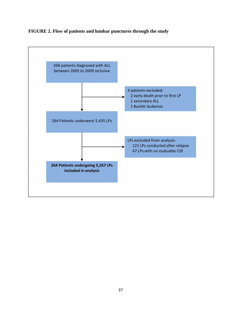
3.1.1 Participants and Procedures

Of the 268 children diagnosed with ALL during the 5-year period, 2 were excluded

because of early death before the first LP, 1 due to a diagnosis of secondary ALL, and 1 due to a

subsequent diagnosis of Burkitt leukemia. The remaining 264 children underwent 5,435 LPs. Of

these, 121 LP observations were excluded as they occurred after a diagnosis of relapse. Sixteen

LPs were documented as being successful but did not have an available CSF RBC count. A

further 31 LPs were failed procedures (0.6%) that also did not have an available CSF RBC count.

Failed LPs were those where documented attempts could not lead to evaluable CSF. These 47

LPs with missing CSF values could not be used in analyses involving the outcome variable of

TLP. They were, however, kept within the dataset as complete exclusion would have affected

variables determined from the previous procedure (such as days since previous LP).

In total, therefore, 264 children undergoing 5267 LPs were included in the final analysis.

The mean number of evaluable LPs was 20.0, and ranged from 1 to 31 per child. The flow of

patients and procedures through the study are shown in Figure 2.

3.1.2 Characteristics

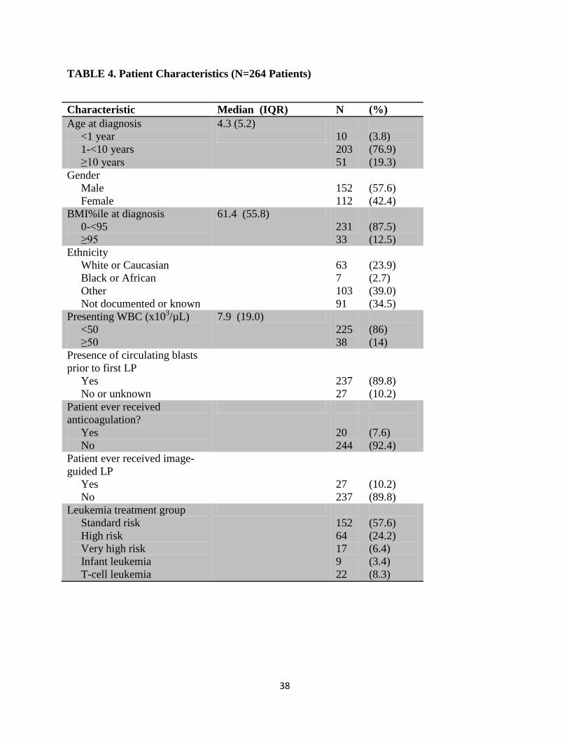
The demographic and disease characteristics for 264 children are shown in Table 4.

These characteristics include time-invariant variables or the value of time-varying covariates at

the day of the first LP. As all continuous variables were non-normally distributed, they are

presented with median and interquartile range.

36

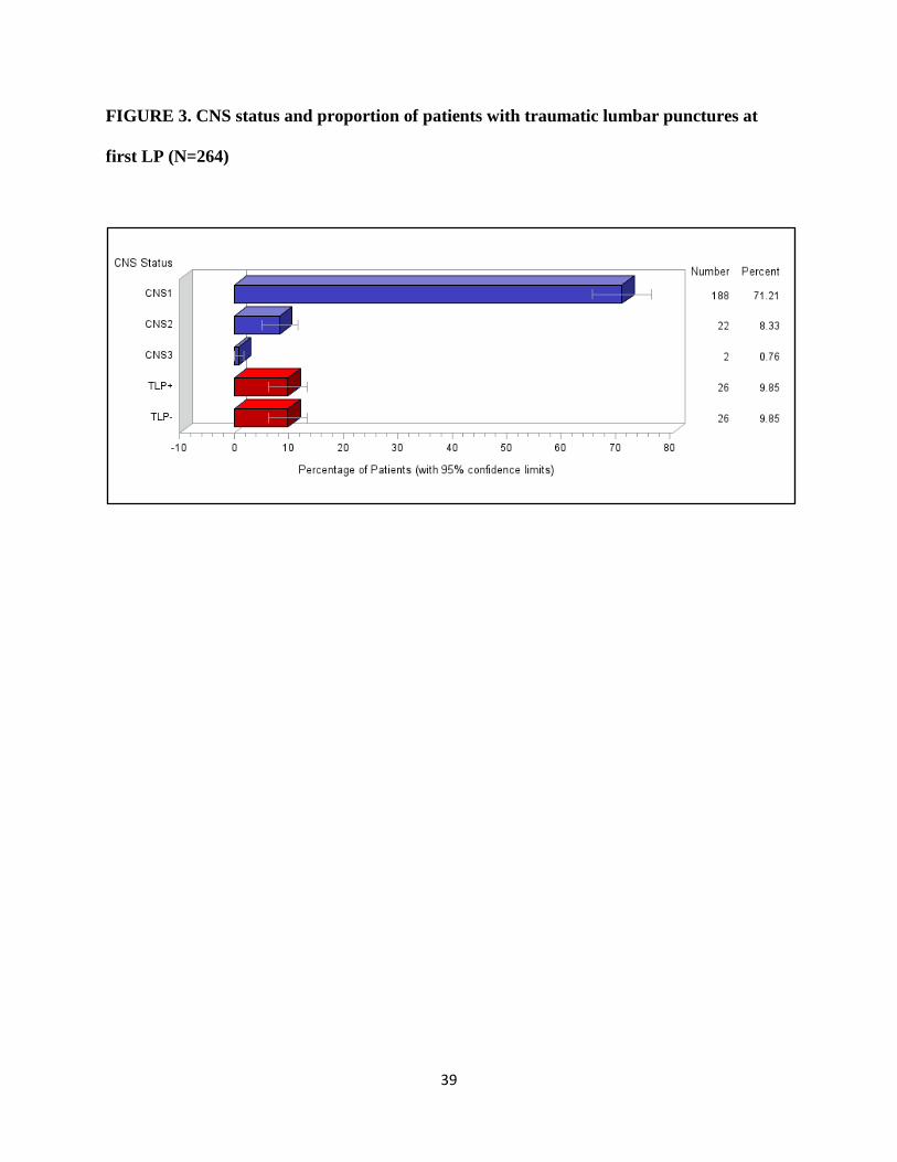
3.1.3 Primary Outcome: Traumatic Lumbar Punctures

Among all 5267 evaluable LPs, there were 943 (17.9%) TLPs. Among the 264 first LPs,

there were 52 (19.7%) TLPs. There were 26 (9.8%) TLP+ containing blasts, and 26 TLP-

containing no blasts. The distribution of CNS status using the SJCRH system are shown in

Figure 3. Of the 26 TLP+ patients, 16 required the treating physician to use the Steinherz-Bleyer

formula to determine the COG CNS status, and 10 could be classified as CNS2 without the

formula.

37

FIGURE 2. Flow of patients and lumbar punctures through the study

268 patients diagnosed with ALL between 2005 to 2009 inclusive

264 Patients underwent 5,435 LPs

264 Patients undergoing 5,267 LPs included in analysis

4 patients excluded: 2 early death prior to first LP 1 secondary ALL 1 Burkitt leukemia

LPs excluded from analysis: 121 LPs conducted after relapse 47 LPs with no evaluable CSF

38

TABLE 4. Patient Characteristics (N=264 Patients)

Characteristic Median (IQR) N (%) Age at diagnosis <1 year 1-<10 years ≥10 years

4.3 (5.2)

10 203 51

(3.8) (76.9) (19.3)

Gender Male Female

152 112

(57.6) (42.4)

BMI%ile at diagnosis 0-<95 ≥95

61.4 (55.8) 231 33

(87.5) (12.5)

Ethnicity White or Caucasian Black or African Other Not documented or known

63 7 103 91

(23.9) (2.7) (39.0) (34.5)

Presenting WBC (x103/µL) <50 ≥50

7.9 (19.0) 225 38

(86) (14)

Presence of circulating blasts prior to first LP Yes No or unknown

237 27

(89.8) (10.2)

Patient ever received anticoagulation? Yes No

20 244

(7.6) (92.4)

Patient ever received image-guided LP Yes No

27 237

(10.2) (89.8)

Leukemia treatment group Standard risk High risk Very high risk Infant leukemia T-cell leukemia

152 64 17 9 22

(57.6) (24.2) (6.4) (3.4) (8.3)

39

FIGURE 3. CNS status and proportion of patients with traumatic lumbar punctures at

first LP (N=264)

40

3.2 Inferential Statistics

3.2.1 Collinearity and Correlations

No two covariates were collinear as per VIF and tolerance criteria. Predictor variables

that had the highest Pearson correlation coefficients included phase of treatment and time since

previous LP (0.49); and platelet count and previous platelet counts (0.25), as shown in Table 5

below.

TABLE 5. Pearson Correlation Coefficients*

Age BMI Phase Days Prior TLP

Platelet Prior Platelet

Age -0.07 0.016 0.012

-0.15 0.10 0.09

BMI -0.07 -0.06 -0.03 -0.07 -0.04 -0.02

Phase 0.016 -0.06 0.49 (<0.001)

-0.10 -0.04 0.21

Days 0.012 -0.03 0.49 (<0.001)

-0.09 0.19 0.17

Prior TLP

-0.15 -0.07 -0.10 -0.09 -0.01 -0.06

Platelet 0.10 -0.04 -0.04 0.19 -0.01 0.25 (<0.001)

Prior Platelet

0.09 -0.02 0.21 0.17 -0.06 0.25 (<0.001)

*P-values shown if coefficient >0.20

41

3.2.2 Model Building

From the list of 13 potential predictor variables listed in Table 3, nine were tested in the

repeated-measures multivariable regression analyses. Initial WBC count and coagulation tests

(INR/PTT) were excluded as they were relevant only to first LPs and were not significantly

associated with first LPs being traumatic. Phase of treatment, although significant in univariate

analyses, was excluded due to its high correlation with days since previous LP. The covariate

ethnicity was difficult to measure. In about one-third of our cases, we could not find any

documentation of ethnicity, and in many other situations found it difficult to classify. Therefore

ethnicity was not further examined as a predictor variable in regression modeling.

The results for univariate and multivariable regression modeling using each of five

methods is shown in Tables 6 to 10. Variables to be included in multivariable models were

selected using backward elimination. The final multivariable models are displayed comparatively

in Table 11. For models that utilized between-subject comparisons (all except fixed effects), the

same five variables were selected using automated or manual backward elimination procedures.

These variables included age at LP (1-<10 years versus < 1 or ≥ 10 years), BMI percentile (≥ 95

versus < 95), platelet count at LP (over 100 x103/L versus 0-50, 51-75 or 76-100 x x103/L), days

since the prior LP (≥16 vs 0-3, 4-7 or 8-15 days), and a preceding TLP.

Both the effect estimates and the confidence intervals produced by each of these methods

were very similar across all covariates, even when accounting for repeated measures was ignored

as in the conventional logistic regression model. The confidence intervals for the conventional

model were only slightly larger than for the GEE model. The effect estimates and CIs produced

by GEE and random effects were slightly different in univariate analysis but became nearly

equivalent in multivariable analysis.

42

In the fixed effects univariate model, platelet count at LP, platelet count at previous LP,

days since previous LP and operator position (radiologist versus oncologist) were significant. In

multivariable analysis, only days since prior LP and operator (radiologist versus oncologist)

remained, and the effect of radiology was seen to reduce the odds of TLP. In total, 27 children

underwent 233 LPs under radiologic guidance. This latter variable was not selected in any other

model. In general, the fixed effects method produced much larger confidence intervals than the

other methods. As expected, it did not produce any estimate for the time-invariant variable, sex.

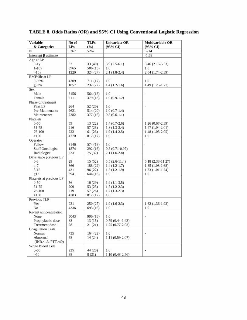
43

TABLE 8. Odds Ratios (OR) and 95% CI Using Conventional Logistic Regression

Variable & Categories

No of LPs

TLPs (%)

Univariate OR (95% CI)

Multivariable OR (95% CI)

N 5267 5267 5214 Intercept β estimate -1.69 Age at LP 0-1y 1-10y >10y

82 3965 1220

33 (40) 586 (15) 324 (27)

3.9 (2.5-6.1) 1.0 2.1 (1.8-2.4)

3.46 (2.16-5.53) 1.0 2.04 (1.74-2.39)

BMI%ile at LP 0-95% ≥95%

4209 1057

711 (17) 232 (22)

1.0 1.4 (1.2-1.6)

1.0 1.49 (1.25-1.77)

Sex Male Female

3156 2111

564 (18) 379 (18)

1.0 1.0 (0.9-1.2)

-

Phase of treatment First LP Pre-Maintenance Maintenance

264 2621 2382

52 (20) 514 (20) 377 (16)

1.0 1.0 (0.7-1.4) 0.8 (0.6-1.1)

-

Platelets 0-50 51-75 76-100 >100

59 216 222 4770

13 (22) 57 (26) 61 (28) 812 (17)

1.4 (0.7-2.6) 1.8 (1.3-2.4) 1.9 (1.4-2.5) 1.0

1.26 (0.67-2.39) 1.47 (1.04-2.01) 1.48 (1.08-2.05) 1.0

Operator Fellow Staff Oncologist Radiologist

3146 1874 233

574 (18) 292 (16) 75 (32)

1.0 0.8 (0.71-0.97) 2.1 (1.6-2.8)

-

Days since previous LP 0-3 4-7 8-15 ≥16

29 866 431 3941

15 (52) 188 (22) 96 (22) 644 (16)

5.5 (2.6-11.4) 1.4 (1.2-1.7) 1.5 (1.2-1.9) 1.0

5.18 (2.38-11.27) 1.35 (1.08-1.68) 1.33 (1.01-1.74) 1.0

Platelets at previous LP 0-50 51-75 76-100 >100

56 209 219 4783

16 (29) 53 (25) 57 (26) 817 (17)

1.9 (1.1-3.5) 1.7 (1.2-2.3) 1.7 (1.3-2.3) 1.0

-

Previous TLP Yes No

931 4336

250 (27) 693 (16)

1.9 (1.6-2.3) 1.0

1.62 (1.36-1.93) 1.0

Recent anticoagulation None Prophylactic dose Treatment dose

5043 88 98

906 (18) 13 (15) 21 (21)

1.0 0.79 (0.44-1.43) 1.25 (0.77-2.03)

-

Coagulation Tests Normal Abnormal (INR>1.3, PTT>40)

735 58

164 (22) 14 (24)

1.0 1.11 (0.59-2.07)

-

White Blood Cell 0-50 >50

225 38

44 (20) 8 (21)

1.0 1.10 (0.48-2.56)

-

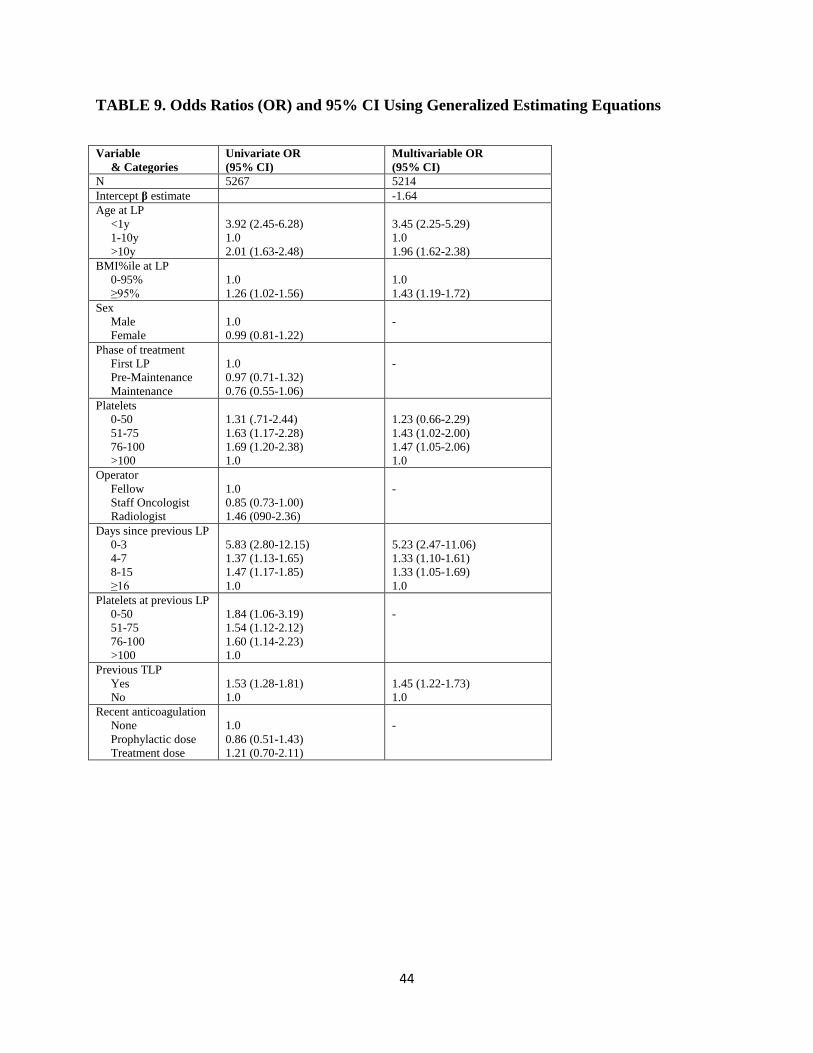
44

TABLE 9. Odds Ratios (OR) and 95% CI Using Generalized Estimating Equations

Variable & Categories

Univariate OR (95% CI)

Multivariable OR (95% CI)

N 5267 5214 Intercept β estimate -1.64 Age at LP <1y 1-10y >10y

3.92 (2.45-6.28) 1.0 2.01 (1.63-2.48)

3.45 (2.25-5.29) 1.0 1.96 (1.62-2.38)

BMI%ile at LP 0-95% ≥95%

1.0 1.26 (1.02-1.56)

1.0 1.43 (1.19-1.72)

Sex Male Female

1.0 0.99 (0.81-1.22)

-

Phase of treatment First LP Pre-Maintenance Maintenance

1.0 0.97 (0.71-1.32) 0.76 (0.55-1.06)

-

Platelets 0-50 51-75 76-100 >100

1.31 (.71-2.44) 1.63 (1.17-2.28) 1.69 (1.20-2.38) 1.0

1.23 (0.66-2.29) 1.43 (1.02-2.00) 1.47 (1.05-2.06) 1.0

Operator Fellow Staff Oncologist Radiologist

1.0 0.85 (0.73-1.00) 1.46 (090-2.36)

-

Days since previous LP 0-3 4-7 8-15 ≥16

5.83 (2.80-12.15) 1.37 (1.13-1.65) 1.47 (1.17-1.85) 1.0

5.23 (2.47-11.06) 1.33 (1.10-1.61) 1.33 (1.05-1.69) 1.0

Platelets at previous LP 0-50 51-75 76-100 >100

1.84 (1.06-3.19) 1.54 (1.12-2.12) 1.60 (1.14-2.23) 1.0

-

Previous TLP Yes No

1.53 (1.28-1.81) 1.0

1.45 (1.22-1.73) 1.0

Recent anticoagulation None Prophylactic dose Treatment dose

1.0 0.86 (0.51-1.43) 1.21 (0.70-2.11)

-

45

TABLE 10. Odds Ratios (OR) and 95% CI Using Random Effects with Generalized Linear

Mixed Models

Variable & Categories

Univariate OR (95% CI)

Multivariable OR (95% CI)

N 5267 5266 Intercept β estimate -1.70 Age at LP <1y 1-10y >10y

4.01 (2.32-6.95) 1.0 2.05 (1.68-2.51)

3.46 (2.06-5.81) 1.0 2.00 (1.66-2.4)

BMI%ile at LP 0-95% ≥95%

1.0 1.28 (1.04-1.58)

1.0 1.44 (1.19-1.75)

Sex Male Female

1.0 0.99 (0.81-1.22)

-

Phase of treatment First LP Pre-Maintenance Maintenance

1.0 0.98 (0.71-1.36) 0.76 (0.55-1.06)

-

Platelets 0-50 51-75 76-100 >100

1.27 (0.66-2.43) 1.65 (1.19-2.29) 1.73 (1.26-2.39) 1.0

1.15 (0.60-2.20) 1.42 (1.01-1.98) 1.49 (1.08-2.07) 1.0

Operator Fellow Staff Oncologist Radiologist

1.0 0.85 (0.72-0.99) 1.39 (0.94-2.08)

-

Days since previous LP 0-3 4-7 8-15 ≥16

6.25 (2.84-13.78) 1.40 (1.16-1.69) 1.46 (1.14-1.89) 1.0

5.13 (2.34-11.25) 1.35 (1.11-1.63) 1.31 (1.02-1.70) 1.0

Platelets at previous LP 0-50 51-75 76-100 >100

1.86 (1.00-3.44) 1.56 (1.11-2.18) 1.59 (1.14-2.21) 1.0

-

Previous TLP Yes No

1.52 (1.27-1.83) 1.0

1.43 (1.19-1.73) 1.0

Recent anticoagulation None Prophylactic dose Treatment dose

1.0 0.83 (0.42-1.66) 1.21 (0.68-2.17)

-

46

TABLE 11. Odds Ratios (OR) and 95% CI Using Fixed Effects with Conditional Logistic

Regression

Variable & Categories

Univariate OR (95% CI)

Multivariable OR (95% CI)

N 5214 Intercept β estimate Age at LP 0-2y 2-9y >9y

2.52 (0.74-8.64) 1.0 1.09 (0.63-1.88)

-

BMI%ile at LP 0-95% ≥95%

1.0 0.99 (0.74-1.32)

-

Sex Male Female

N/A

-

Phase of treatment First LP Pre-Maintenance Maintenance

1.0 0.99 (0.71-1.37) 0.79 (0.56-1.11)

-

Platelets 0-50 51-75 76-100 >100

1.20 (0.61-2.35) 1.45 (1.03-2.03) 1.54 (1.10-2.15) 1.0

-

Operator Fellow Staff Oncologist Radiologist

1.0 0.90 (0.76-1.06) 0.54 (0.31-0.94)

1.0 0.90 (0.77-1.07) 0.55 (0.32-0.95)

Days since previous LP 0-3 4-7 8-15 ≥16

7.02 (2.92-16.88) 1.33 (1.10-1.61) 1.41 (1.08-1.84) 1.0

7.34 (3.05-17.67) 1.31 (1.08-1.58) 1.40 (1.07-1.82) 1.0

Platelets at previous LP 0-50 51-75 76-100 >100

1.78 (0.94-3.37) 1.43 (1.01-2.02) 1.47 (1.04-2.06) 1.0

-

Previous TLP Yes No

1.10 (0.92-1.31) 1.0

-

Recent anticoagulation None Prophylactic dose Treatment dose

1.0 0.90 (0.37-2.18) 1.18 (0.55-2.51)

-

47

TABLE 12. Odds Ratios (OR) and 95% CI Using The Hybrid Method

Variable & Categories

Multivariable OR (95% CI)

N 5249 Intercept β estimate -1.68 Age at LP <1y 1-10y >10y

3.48 (2.10-5.77) 1.0 1.80 (1.49-2.18)

BMI%ile at LP 0-95% ≥95%

1.0 1.35 (1.11-1.63)

Sex Male Female

-

Phase of treatment First LP Pre-Maintenance Maintenance

-

Platelets 0-50 51-75 76-100 >100

1.13 (0.59-2.18) 1.38 (0.99-1.94) 1.43 (1.03-1.98) 1.0

Operator (Oncologist vs Radiologist) Fixed Effects Random Effects

0.56 (0.33-0.96) 2.19 (1.38-3.47)

Days since previous LP 0-3 4-7 8-15 ≥16

5.19 (2.38-11.36) 1.32 (1.09-1.60) 1.32 (1.02-1.71) 1.0

Platelets at previous LP 0-50 51-75 76-100 >100

-

Previous TLP Yes No

1.44 (1.19-1.73) 1.0

Recent anticoagulation None Prophylactic dose Treatment dose

-

48

TABLE 13. Comparison of Models

Variable & Categories

No of LPs

TLPs (%)

Unadjusted Univariate OR

Logistic Regression GEE Random Effects Fixed Effects Hybrid

Age at LP <1y 1-10y >10y

82 3965 1220

33 (40) 586 (15) 324 (27)

3.9 (2.5-6.1) 1.0 2.1 (1.8-2.4)

3.46 (2.16-5.53) 1.0 2.04 (1.74-2.39)

3.45 (2.25-5.29) 1.0 1.96 (1.62-2.38)

3.46 (2.06-5.81) 1.0 2.00 (1.66-2.4)

-

3.48 (2.10-5.77) 1.0 1.80 (1.49-2.18)

BMI at LP 0-95%ile >95%ile

4209 1057

711 (17) 232 (22)

1.0 1.4 (1.2-1.6)

1.0 1.49 (1.25-1.77)

1.0 1.43 (1.19-1.72)

1.0 1.44 (1.19-1.75)

-

1.0 1.35 (1.11-1.63)

Platelets 0-50 51-75 76-100 >100

59 216 222 4770

13 (22) 57 (26) 61 (28) 812 (17)

1.4 (0.7-2.6) 1.8 (1.3-2.4) 1.9 (1.4-2.5) 1.0

1.26 (0.67-2.39) 1.47 (1.04-2.01) 1.48 (1.08-2.05) 1.0

1.23 (0.66-2.29) 1.43 (1.02-2.00) 1.47 (1.05-2.06) 1.0

1.15 (0.60-2.20) 1.42 (1.01-1.98) 1.49 (1.08-2.07) 1.0

-

1.13 (0.59-2.18) 1.38 (0.99-1.94) 1.43 (1.03-1.98) 1.0

Operator Fellow Staff Radiologist

3146 1874 233

574 (18) 292 (16) 75 (32)

1.0 0.8 (0.71-0.97) 2.1 (1.6-2.8)

-

-

-

1.0 0.90 (0.77-1.07) 0.55 (0.32-0.95)

FE: 0.56 (0.33-0.96) RE: 2.19 (1.38-3.47)

Days since prior LP 0-3 4-7 8-15 ≥16

29 866 431 3941

15 (52) 188 (22) 96 (22) 744 (16)

5.5 (2.6-11.4) 1.4 (1.2-1.7) 1.5 (1.2-1.9) 1.0

5.18 (2.38-11.3) 1.35 (1.08-1.68) 1.33 (1.01-1.74) 1.0

5.23 (2.47-11.1) 1.33 (1.10-1.61) 1.33 (1.05-1.69) 1.0

5.13 (2.34-11.3) 1.35 (1.11-1.63) 1.31 (1.02-1.70) 1.0

7.34 (3.05-17.7) 1.31 (1.08-1.58) 1.40 (1.07-1.82) 1.0

5.19 (2.38-11.36) 1.32 (1.09-1.60) 1.32 (1.02-1.71) 1.0

Previous TLP Yes No

931 4336

250 (27) 693 (16)

1.9 (1.6-2.3) 1.0

1.62 (1.36-1.93) 1.0

1.45 (1.22-1.73) 1.0

1.43 (1.19-1.73) 1.0

-

1.44 (1.19-1.73) 1.0

49

3.2.3 Secondary Outcome: Event-Free Survival

The mean length of follow-up was 3.9 years (SD 1.6 years). For 188 children with CNS1

status, the 5-year EFS was 93% (SE±2). For 26 children with TLP+ status, the 5-year EFS was

77% (±8). The difference between these two groups was statistically significant (Log-rank p=

0.002). Kaplan-Meier survival curves are shown in Figure 4.

FIGURE 4. Kaplan-Meier survival curves by CNS status

50

CHAPTER 4: DISCUSSION

4.1 Summary of Main Findings

In our retrospective cohort study of 5267 LPs, we observed an overall TLP rate of 17.9%

and a first TLP rate of 19.7%. In terms of identifying predictors of TLP, we found that among

the random effects model and GEE, the variables independently associated with TLP were age

less than 1 or over 10 years, BMI percentile over 95, platelet count less than 100 x103/µL, fewer

days since the previous LP, and a previous TLP. However, in the fixed effects model, the

variables independently associated with TLP were fewer days since the previous LP, and the use

of image-guidance by a radiologist.

The overall proportion of TLPs in our study is lower than that reported by Howard et al

(29.3%).34 This is likely due to the fact that Howard et al included only the first few LPs per

child, and therefore had a greater proportion of LPs in the intensive phases of treatment where

LPs are performed closer together. It may also be related to the study being conducted during an

era when procedural sedation was not routinely used, and when junior trainees such as medical

students and residents also performed LPs on children with ALL. Nevertheless, given the

significant consequences of TLPs in ALL, we believe that our proportion of TLPs is still high

and that further attempts at minimizing this complication are still needed.

4.2 Factors Predictors of TLP

The proportion of TLP was higher among infants than children 1-<10 years of age in our

study. This may be due to the technical challenges of performing the procedure within a smaller

51

anatomic space. Due to the shallower distances between the subarachnoid space and the posterior

venous plexus, the infant spine offers a narrower margin of error. Thus even small

miscalculations in estimating distance or angle of needle insertion, coupled with the larger

relative size of the LP needle to the anatomic structures, may increase the chance of blood vessel

laceration. The proportion of TLP was also significantly higher among children older than 10

years compared to those between 1-10 years of age. A different set of technical challenges

probably account for this observation. As children grow older and larger, the distance between

the skin and the spinous processes increases, which makes the spinous processes and thus the

optimal site of needle insertion more difficult to visualize and palpate. With increased distance,

any deviation from the ideal angle at the skin puncture site becomes amplified. Lastly, older

children often require longer needles which are more technically challenging to use. Longer

needles can curve or bend on insertion and are therefore harder to direct in a straight trajectory.

Obesity was also significantly associated with TLP. The reasons for this may be similar

as for older age. Procedure landmarks are harder to palpate in the presence of obesity, and needle

distances are greater. Shah et al found that being unable to visualize (let alone palpate) the

spinous processes for adults in the emergency room was a risk factor for traumatic LPs.40 This

variable was not assessed by Howard et al.34

Age and obesity are both patient-related factors. They are not modifiable at the time of

the LP. However, they are useful as predictor variables in that they can identify those subsets of

patients with a higher risk of TLP. Such risk-stratification would be important to allow directing

interventions to reduce TLP to those patients who are most likely to benefit.

A lower platelet count before the LP was a modifiable risk factor, as children with

thrombocytopenia can be given a platelet transfusion prior to their procedure. We found that the

52

risk of a TLP is significantly associated with all platelet counts under 100 x 103/µL.

Interestingly, patients in all categories with platelet counts less than 100 x 103/µL had an

increased risk, and the risk was not substantially different across the categories below this

threshold. These results are remarkably similar to those identified by Howard et al. The authors

of that study recommended that “in those settings in which traumatic LP is particularly

undesirable and the benefit of transfusion outweighs the disadvantages, such as the diagnostic LP

in a child with ALL and circulating leukemic cells, platelet transfusion for a count of 100 x

103/µL or lower is warranted.”34 Therefore, at SJCRH all children with newly diagnosed ALL

are transfused if their platelet count is below this threshold prior to their first LP.61 Our findings

support this practice. This same threshold was not included as a recommendation in a recent

Canadian platelet transfusion guideline for pediatric cancer patients.62

The proportion of TLPs was significantly higher when a prior LP was performed within

the preceding 15 days, and also if the prior LP was itself traumatic. Both these variables can be

regarded as “lag” variables. Although they are not themselves clinically useful, they are

important to include as potential confounders in a repeated-measures study. By adjusting for

them within the multivariable model, the results obtained from sequential LPs can be more

meaningfully applied to understanding predictors of TLPs.

4.3 Pertinent Negative Findings

In addition to these five identified risk factors, there were two pertinent negative findings

of our study worth highlighting.

First, although TLP rates varied widely among different operators, we found no

significant difference in the rate of TLPs between oncology fellows and staff. Therefore, rather

53

than restrict fellows from performing first LPs, institutions should consider identifying their best

performers within all positions who can be called upon to perform first LPs, especially in

children with higher risk of TLP.

Secondly, our study is the first to look for an association between the use of recent

anticoagulation therapy and the proportion of TLPs. No significant association was found. This

result is important because approximately 5% of all children with ALL will experience a

thrombotic event requiring anticoagulation with either heparin or LMWH.63 Large bleeds within

the spinal canal, known as spinal hematomas, are a rare but devastating complication of LPs that

can lead to paraplegia or death.64,65 Consequently, at SickKids, our institutional practice is to

hold unfractionated heparin for 4 hours and LMWH for 24 hours prior to an LP without requiring

coagulation testing. Our results suggest that this practice is sufficient to prevent even

microscopic bleeding.

4.4 Survival Analysis

Consistent with previous studies,22-24 we found a significant reduction in EFS for children

with TLP+ compared to those who had CNS1 status. This shows that TLP+ continues to be a

prognostic factor even in the context of contemporary therapy with additional treatments given to

these children. This lends further importance to the need to reduce first TLPs to as low as

possible in children with ALL.

4.5 Comparison of Repeated-Measures Analysis Methods

The five risk factors highlighted above were all identified as being the most significant

factors in models fitted using either conventional logistic regression, GEE or random effects

54

mixed models. Indeed, both the effect estimates and the confidence intervals produced by each of

these methods were very similar across all covariates. The similarity of findings across the

different regression methods means that our results are robust to the choice of statistical method.

It also suggests that within-patient correlations and unobserved heterogeneity were not

significant factors within this dataset.

In going from a model that incorrectly ignored dependence among individuals to those

that accounted for it, no substantial change in results was seen. Generally speaking, regression

models that ignore correlation tend to overestimate the standard errors of time-varying

covariates, while the effect on the size of the coefficient estimates is less pronounced.50,55 While

the confidence intervals may be slightly wider for the conventional logistic regression model

compared to GEE in our study, the differences are very subtle. This might suggest that residual

intra-individual correlation was not a strong factor in this setting. Lastly, it may perhaps imply

that TLP risk does not tend on average to cluster within individuals, and hence that there is either

not much variation in TLP risk between individuals and/or that most variation in TLP proportion

is for reasons extrinsic to the individual.

The effect estimates and CIs produced by GEE and random effects were again equivalent.

This reinforces the similarities between these two models in spite of the very different underlying

estimation methods.46 We did not observe any heterogeneity shrinkage in the GEE model relative

to the random effects model, which suggests that unobserved heterogeneity was minimal. Indeed,

the GEE estimates tended to be slightly smaller than the corresponding random effects estimates

in univariate analysis, but more similar in multivariable analysis as the unobserved heterogeneity

was reduced by the addition of covariates. However, this again leads us to conclude that

55

variation in subject-specific effects is small. Indeed, while TLP proportion between individuals

does vary, it tends to do so mainly within the range of 10% to 30%.

In contrast, the fixed effects model led to very different results. As might have been

expected, no significant association for age at LP or BMI percentile was seen. This is because

these variables do not change much over the course of 3 years of observation, especially when

they are categorized at cut-points. They in effect behaved as time-invariant variables when

restricted to just one individual. The number of days since prior LP remained a strong predictor,

but had much larger confidence intervals, as would be expected. Since fixed effects discards data

for any patient whose outcome variable does not change across predictor categories, it makes

inefficient use of the data and thus works with effectively smaller sample sizes.

Furthermore, in the fixed effects method one additional factor was noted to be significant:

the use of fluoroscopic image-guidance by an interventional radiologist. In our cohort, 27

children underwent 233 LPs under fluoroscopy. These were all children who were referred to the

interventional radiologist by the patient’s oncology team after either failed or repeatedly difficult

LPs. Moreover, these procedures often occurred within a few days after a prior LP attempt. One

would therefore expect to see susceptibility bias and/or confounding-by-indication in this group

of children. Indeed, it is instructive to observe how the estimated effect of this variable changed

across the different analytic methods. In unadjusted analysis, the image-guided LPs were

traumatic twice as often as all other LPs, with an overall rate of 32% and an OR of 2.1. In

univariate GEE adjusting only for correlations, the OR declined to 1.39 and lost statistical

significance. It further declined to 1.16 in multivariable GEE accounting for all other significant

covariates, likely due mostly to the added adjustment for days since prior LP (data not shown).

Lastly, in the fixed effects analysis, the effect of image-guidance reversed direction and was seen

56

to be significantly protective against TLP, with an OR of 0.55. The fixed effects method balances

unobserved but stable covariates and uses each patient as their own control.48 This suggests that

among the small group of patients selected for a referral to image-guidance, there is an intrinsic

but un-measured variable that predisposes them to a higher rate of TLP. Within these patients,

the use of image-guidance can reduce the risk of TLP.

After comparing the strengths and limitations of all models, we selected the GEE model

for final presentation. The differences between GEE and the random effects model are minimal,

and we based our decision on the fact that we are most interested in population-averaged rather

than subject-specific effects. The population-averaged coefficients allow users to estimate the

average change in the proportion of the outcome if modification of a risk factor was applied

across all patients.50

4.6 Study Limitations

Our study had several limitations. As a retrospective study, recording of covariates was

limited to those which were documented as part of routine clinical care. Therefore, several

potential predictor variables could not be assessed. For example, we could not assess the

potential impact of depth of anesthesia or degree of patient movement, the positioning of the

patient during the procedure, the width or length of needle used for the LP, or particular operator

practices such as removing the stylet. However, these particular variables would not be expected

to vary much within our cohort, as most procedures are performed within consistent parameters.

Unlike Shah et al,40 we could not assess whether operators were able to visualize or palpate the

spinous landmarks or whether this variable correlated with obesity. Furthermore, unlike Glatstein

57

et al,41 we could not assess whether multiple attempts increased the risk of TLP, as operators did

not document their number of attempts except in rare cases.

As with all non-experimental research, it is always possible that other important

explanatory variables were omitted as a result of not having been considered at all. Indeed, the

results of our fixed effects analysis on image-guidance does strongly suggest that some

unmeasured variable(s) accounts for a high proportion of TLP in at least a subgroup of children.

Lastly, a limitation of our study is that SickKids is a large tertiary-care referral center.

Therefore our results may not be generalizable to smaller or non-academic centers.

4.7 Study Strengths

A strength of our study is its large sample size. Furthermore, those covariates which were

included for the study had very low rates of missing data. Since nearly all LPs for childhood

cancer patients at SickKids are performed under deep sedation, documentation for procedures is

generally of a high quality. Only 47 (0.9%) LPs had missing outcome data (no CSF RBC count)

and only another 53 LPs (1.0%) had data missing on covariate values for the final model.

Another strength of this study was our use and comparison of multiple regression

methods for repeated-measures, which allowed us to gain better insights into the data and present

the most suitable multivariable model. Since results were consistent across all models that

performed within-person comparisons, the results of our analysis were robust to the choice of

method.

Our study had broad inclusion criteria and included all LPs for all children with any type

of ALL. Therefore, the study results should be generalizable to other large pediatric oncology

58

institutions where the routine practices regarding deep sedation and operator experience are

similar to ours.

4.8 Future Research

The findings from this study provide a foundation for future research. Image-guidance

may have the potential to reduce TLPs in children with particular susceptibility, and this

hypothesis should be further investigated. We are currently planning a study to determine

whether ultrasound-guidance performed in the oncology procedure room can reduce the

proportion of TLPs. Another future direction could be to determine prospectively whether

implementation of the clinical recommendations from this study, such as platelet transfusion

thresholds, identification of selected operators for first LPs, and/or image-guidance, are able to

reduce the proportion of first TLPs over time.

Lastly, the dataset in this study led to similar conclusions regardless of whether

conventional logistic regression, random effects, or GEE was used, and thus the relative

strengths and weaknesses of each method were not specifically highlighted. Future research

could therefore utilize simulations with varying degrees of intra-individual correlation and

unobserved heterogeneity in order to determine the relative strengths, bias, and efficiency of

each method under specific conditions. This could provide further guidance to researchers on

which method to use under different circumstances.

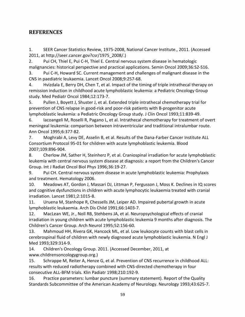
59

REFERENCES

1. SEER Cancer Statistics Review, 1975-2008, National Cancer Institute., 2011. (Accessed 2011, at http://seer.cancer.gov?csr/1975_2008/.) 2. Pui CH, Thiel E, Pui C-H, Thiel E. Central nervous system disease in hematologic malignancies: historical perspective and practical applications. Semin Oncol 2009;36:S2-S16. 3. Pui C-H, Howard SC. Current management and challenges of malignant disease in the CNS in paediatric leukaemia. Lancet Oncol 2008;9:257-68. 4. Hvizdala E, Berry DH, Chen T, et al. Impact of the timing of triple intrathecal therapy on remission induction in childhood acute lymphoblastic leukemia: a Pediatric Oncology Group study. Med Pediatr Oncol 1984;12:173-7. 5. Pullen J, Boyett J, Shuster J, et al. Extended triple intrathecal chemotherapy trial for prevention of CNS relapse in good-risk and poor-risk patients with B-progenitor acute lymphoblastic leukemia: a Pediatric Oncology Group study. J Clin Oncol 1993;11:839-49. 6. Iacoangeli M, Roselli R, Pagano L, et al. Intrathecal chemotherapy for treatment of overt meningeal leukemia: comparison between intraventricular and traditional intralumbar route. Ann Oncol 1995;6:377-82. 7. Moghrabi A, Levy DE, Asselin B, et al. Results of the Dana-Farber Cancer Institute ALL Consortium Protocol 95-01 for children with acute lymphoblastic leukemia. Blood 2007;109:896-904. 8. Cherlow JM, Sather H, Steinherz P, et al. Craniospinal irradiation for acute lymphoblastic leukemia with central nervous system disease at diagnosis: a report from the Children's Cancer Group. Int J Radiat Oncol Biol Phys 1996;36:19-27. 9. Pui CH. Central nervous system disease in acute lymphoblastic leukemia: Prophylaxis and treatment. Hematology 2006. 10. Meadows AT, Gordon J, Massari DJ, Littman P, Fergusson J, Moss K. Declines in IQ scores and cognitive dysfunctions in children with acute lymphocytic leukaemia treated with cranial irradiation. Lancet 1981;2:1015-8. 11. Uruena M, Stanhope R, Chessells JM, Leiper AD. Impaired pubertal growth in acute lymphoblastic leukaemia. Arch Dis Child 1991;66:1403-7. 12. MacLean WE, Jr., Noll RB, Stehbens JA, et al. Neuropsychological effects of cranial irradiation in young children with acute lymphoblastic leukemia 9 months after diagnosis. The Children's Cancer Group. Arch Neurol 1995;52:156-60. 13. Mahmoud HH, Rivera GK, Hancock ML, et al. Low leukocyte counts with blast cells in cerebrospinal fluid of children with newly diagnosed acute lymphoblastic leukemia. N Engl J Med 1993;329:314-9. 14. Children's Oncology Group. 2011. (Accessed December, 2011, at www.childrensoncologygroup.org.) 15. Schrappe M, Reiter A, Henze G, et al. Prevention of CNS recurrence in childhood ALL: results with reduced radiotherapy combined with CNS-directed chemotherapy in four consecutive ALL-BFM trials. Klin Padiatr 1998;210:192-9. 16. Practice parameters: lumbar puncture (summary statement). Report of the Quality Standards Subcommittee of the American Academy of Neurology. Neurology 1993;43:625-7.

60

17. Rech A, de Carvalho GP, Meneses CF, Hankins J, Howard S, Brunetto AL. The influence of traumatic lumbar puncture and timing of intrathecal therapy on outcome of pediatric acute lymphoblastic leukemia. Pediatr Hematol Oncol 2005;22:483-8. 18. Conter V, Arico M, Valsecchi MG, et al. Extended intrathecal methotrexate may replace cranial irradiation for prevention of CNS relapse in children with intermediate-risk acute lymphoblastic leukemia treated with Berlin-Frankfurt-Munster-based intensive chemotherapy. The Associazione Italiana di Ematologia ed Oncologia Pediatrica. J Clin Oncol 1995;13:2497-502. 19. Nachman J, Sather HN, Cherlow JM, et al. Response of children with high-risk acute lymphoblastic leukemia treated with and without cranial irradiation: a report from the Children's Cancer Group. J Clin Oncol 1998;16:920-30. 20. Pui CH, Campana D, Pei D, et al. Treating childhood acute lymphoblastic leukemia without cranial irradiation. N Engl J Med 2009;360:2730-41. 21. Pappano D. "Traumatic tap" proportion in pediatric lumbar puncture. Pediatric Emergency Care 2010;26:487-9. 22. Gajjar A, Harrison PL, Sandlund JT, et al. Traumatic lumbar puncture at diagnosis adversely affects outcome in childhood acute lymphoblastic leukemia. Blood 2000;96:3381-4. 23. Burger B, Zimmermann M, Mann G, et al. Diagnostic cerebrospinal fluid examination in children with acute lymphoblastic leukemia: significance of low leukocyte counts with blasts or traumatic lumbar puncture. J Clin Oncol 2003;21:184-8. 24. te Loo DM, Kamps WA, van der Does-van den Berg A, et al. Prognostic significance of blasts in the cerebrospinal fluid without pleiocytosis or a traumatic lumbar puncture in children with acute lymphoblastic leukemia: experience of the Dutch Childhood Oncology Group. J Clin Oncol 2006;24:2332-6. 25. Larson S, Schall G, Di Chrio G. The influence of previous lumbar puncture and pneumoencephalography on the incidence of unsuccessful radioisotope cisternography. Journal of Nuclear Medicine 1971;12. 26. Chordas C. Post-dural puncture headache and other complications after lumbar puncture. J Pediatr Oncol Nurs 2001;18:244-59. 27. Holdsworth MT, Raisch DW, Winter SS, et al. Pain and distress from bone marrow aspirations and lumbar punctures. Ann Pharmacother 2003;37:17-22. 28. Ebinger F, Kosel C, Pietz J, Rating D. Headache and backache after lumbar puncture in children and adolescents: A prospective study. Pediatrics 2004;113:1588-92. 29. Eskey CJ, Ogilvy CS. Fluoroscopy-guided lumbar puncture: Decreased frequency of traumatic tap and implications for the assessment of CT-negative acute subarachnoid hemorrhage. American Journal of Neuroradiology 2001;22:571-6. 30. Yu SD, Chen MY, Johnson AJ. Factors associated with traumatic fluoroscopy-guided lumbar punctures: a retrospective review. Ajnr: American Journal of Neuroradiology 2009;30:512-5. 31. Sidhu M, Coley B, Goske M, et al. Image Gently, Step Lightly: increasing radiation dose awareness in pediatric interventional radiology. Pediatric Radiology 2009;39:1135-8. 32. Chong AL, Grant R, Ahmed B, Thomas K, Connolly BL, Greenberg M. Imaging in pediatric patients: Time to think again about surveillance. Pediatr Blood Cancer 2010;55:407-13.

61

33. Miksys N, Gordon CL, Thomas K, Connolly BL. Estimating effective dose to pediatric patients undergoing interventional radiology procedures using Anthropomorphic Phantoms and MOSFET dosimeters. Am J Roentgenol 2010;194:1315-22. 34. Howard SC, Gajjar AJ, Cheng C, et al. Risk factors for traumatic and bloody lumbar puncture in children with acute lymphoblastic leukemia. Jama 2002;288:2001-7. 35. Shah K, Richard KM, Nicholas S, Edlow J. Incidence of traumatic lumbar puncture. Academic Emergency Medicine 2003;10:151-4. 36. Molina A, Fons J. Factors associated with lumbar puncture success. Pediatrics 2006;118:842-4; author reply 4. 37. Kaushal HS, Daniel M, Jeffrey S, Jonathan AE. Predicting difficult and traumatic lumbar punctures. The American journal of emergency medicine 2007;25:608-11. 38. Nigrovic L, Kuppermann N, Neuman M. Risk Factors for Traumatic or Unsuccessful Lumbar Punctures in Children. Annals of emergency medicine 2007;49:762-71. 39. Nigrovic LE, McQueen AA, Neuman MI. Lumbar Puncture Success Rate Is Not Influenced by Family-Member Presence. Pediatrics 2007;120:e777-82. 40. Shah K, McGillicuddy D, Spear J, Edlow J. Predicting difficult and traumatic lumbar punctures. The American journal of emergency medicine 2007;25:608-11. 41. Glatstein MM, Zucker-Toledano M, Arik A, Scolnik D, Oren A, Reif S. Incidence of traumatic lumbar puncture: experience of a large, tertiary care pediatric hospital. Clin Pediatr (Phila) 2011;50:1005-9. 42. Airhart A, Doyle J, Airhart C, Abla O, Alexander S. Assessment of pediatric haematology/oncology fellows' training in the performance of lumbar punctures [abstract]. Pediatr Blood Cancer 2009;52:721. 43. Ljungman G, Gordh T, Sorensen S, Kreuger A. Lumbar puncture in pediatric oncology: conscious sedation vs. general anesthesia. Med Pediatr Oncol 2001;36:372-9. 44. Gardiner JC, Luo Z, Roman LA. Fixed effects, random effects and GEE: What are the differences? Statistics In Medicine 2009;28:221-39. 45. Edwards LJ. Modern statistical techniques for the analysis of longitudinal data in biomedical research. Pediatric Pulmonology 2000;30:330-44. 46. Fitzmaurice GM, Laird NM, Ware JH. Applied Longitudinal Analysis. New Jersey: Wiley; 2011. 47. Singer JD, Willett JB. Applied Longitudinal Data Analysis: Modeling Change and Event Occurrence. Madison Avenue, New York: Oxford University Press, Inc; 2003. 48. Allison PD. Fixed Effects Regression Methods for Longitudinal Data: Using SAS. Cary, NC: SAS Institute Inc; 2005. 49. Lipsitz RS, Fitzmaurice GM. Sample size for repeated measures studies with binary responses. Statistics In Medicine 1994;13:1233-9. 50. Hu FB, Goldberg J, Hedeker D, Flay BR, Pentz MA. Comparison of population-averaged and subject-specific approaches for analyzing repeated binary outcomes. American Journal of Epidemiology 1998;147:694-703. 51. Locascio JJ, Atri A. An overview of longitudinal data analysis methods for neurological research. Dement Geriatr Cognitive Disorders Extra 2011;1:330-57.

62

52. Cheng J, Edwards LJ, Maldonado-Molina MM, Komro KA, Milluer KE. Real longitudinal data analysis for real people: Building a good enough mix model. Statistics In Medicine 2010;29:504-20. 53. Liang KY, zeger SL. Longitudinal data analysis using generalized linear models. Biometrika 1986;73:13-22. 54. Pan W. Akaike's information criterion in generalized estimating equations Biometrcs 2001;57:120-5. 55. Allison PD. Logistic Regression Using the SAS System: Theory and Application. . Cary NC: SAS Institute Inc.; 1999. 56. A SAS Program for the CDC Growth Charts. Centers for Disease Control and Prevention, 2011. (Accessed March 2012, at http://www.cdc.gov/nccdphp/dnpao/growthcharts/resources/sas.htm.) 57. Barlow SE. Expert committee recommendations regarding the prevention, assessment, and treatment of child and adolescent overweight and obesity: Summary report. Pediatrics 2007;120:S164-S92. 58. Peduzzi P, Concato J, Kemper E, Holford T, Feinstein A. A simulation study of the number of events per variable in logistic regression analysis. Journal of Clinical Epidemiology 1996;49:1373-9. 59. Concato J, Peduzzi P, Holford T, et al. Importance of events per independent variable in proportional hazards analysis. I. Background, goals, and general strategy. Journal of Clinical Epidemiology 1995;48:1495-501. 60. Allison PD. Survival Analysis Using SAS: A Pratcical Guide. Second ed. Cary NC: SAS Institute Inc; 2010. 61. Howard SC, Gajjar A, Ribeiro RC, et al. Safety of lumbar puncture for children with acute lymphoblastic leukemia and thrombocytopenia. Jama 2000;284:2222-4. 62. Guideline for platelet transfusion thresholds for pediatric hematology/oncology patients: Complete reference guide. The C17 Guidelines Committee, 2010. (Accessed March 2011, at http://www.c17.ca/index.php?cID=86.) 63. Caruso V, Iacoviello L, Di Castelnuovo A, et al. Thrombotic complications in childhood acute lymphoblastic leukemia: a meta-analysis of 17 prospective studies comprising 1752 pediatric patients. Blood 2006;108:2216-22. 64. Kreppel D, Antoniadis G, Seeling W. Spinal hematoma: a literature survey with meta-analysis of 613 patients. Neurosurgical Review 2003;26:1-49. 65. van Veen JJ, Nokes TJ, Makris M. The risk of spinal haematoma following neuraxial anaesthesia or lumbar puncture in thrombocytopenic individuals. British Journal of Haematology 2010;148:15-25.

63

APPENDICES

APPENDIX I. Approach to Classifying TLP+ Status Varies Between SJCRH and COG

Systems

In the SHCRH system, a TLP+ is defined as its own CNS group without further attempt to

distinguish the possible underlying status:

CNS1 Absence of blasts in CSF, and <10 RBC/µL

CNS2 <5 WBC/µL, <10 RBC/µL, blasts

CNS3 ≥5 WBC, <10 RBC/µL, blasts

TLP- Absence of blasts in CSF, and ≥10 RBC/µL

TLP+ ≥10 RBC/µL, blasts

In contrast, the COG system uses the following Steinherz/Bleyer algorithm for all patients with

TLP+ to try and distinguish between underlying CNS2 and CNS3 disease:

CSF WBC > 2X CSF RBC Blood RBC

Blood WBC

A patient whose CSF WBC/RBC is 2x greater than the blood WBC/RBC ratio is considered to

have CNS3 disease at diagnosis.

64

APPENDIX II. Risk Group Definitions for B-cell Precursor ALL

Risk Group Definition Standard Risk Age 1.0 to 9.99 years

WBC < 50,000/µL Standard risk-low Not CNS2 or CNS3 or testicular disease

Favourable genetics Day 8 peripheral blood MRD <0.01% Day 29 bone marrow MRD <0.01% No steroid pretreatment

Standard-risk average No unfavourable genetics Day 8 peripheral blood MRD ≥ 0.01% or CNS2 status Day 29 bone marrow MRD < 0.01% No CNS3 or testicular disease

High-Risk Age <1 or ≥10 years WBC ≥50,000/µL CNS3 or testicular disease Steroid pretreatment

Very High-Risk ALL BCR-ABL fusion Hypodiploidy Induction failure MLL rearrangement and slow-early response after induction