Materiales de ConstruCCión

Vol. 69, Issue 334, April–June 2019, e190ISSN-L: 0465-2746

https://doi.org/10.3989/mc.2019.07018

Predicting the Mechanical Properties of Concrete Using Intelligent Techniques to Reduce CO2 Emissions

H. H. Ghayeba*, H. A. Razaka, N.H. R. Sulonga, A. N. Hanoonb, F. Abutahac, H. A. Ibrahima, M. Gordana, M. F. Alnahhala

a. Department of Civil Engineering, Faculty of Engineering, University of Malaya, 50603 Kuala Lumpur, Malaysia.b. The Engineering Affairs Department, University of Baghdad, Baghdad, Iraq.

c. Faculty of Civil Engineering, Istanbul Technical University, Maslak, Istanbul 34469, Turkey.*eng_hhg@yahoo.com

Received 9 July 2018 Accepted 27 November 2018 Available on line 7 May 2019

ABSTRACT: The contribution to global CO2 emissions from concrete production is increasing. In this paper, the effect of concrete mix constituents on the properties of concrete and CO2 emissions was investigated. The tested materials used 47 mixtures, consisting of ordinary Portland cement (OPC) type I, coarse aggregate, river sand and chemical admixtures. Response surface methodology (RSM) and particle swarm optimisation (PSO) algorithms were employed to evaluate the mix constituents at different levels simultaneously. Quadratic and line models were produced to fit the experimental results. Based on these models, the concrete mixture necessary to achieve optimum engineering properties was found using RSM and PSO. The resulting mixture required to obtain the desired mechanical properties for concrete was 1.10-2.00 fine aggregate/cement, 1.90-2.90 coarse aggregate/cement, 0.30-0.4 water/cement, and 0.01-0.013 chemical admixtures/cement. Both methods had over 94% accuracy, compared to the experimental results. Finally, by employing RSM and PSO methods, the number of experimental mixtures tested could be reduced, saving time and money, as well as decreasing CO2 emissions.

KEYWORDS: CO2 emission; Mechanical properties of concrete; Optimum mix design; Particle swarm optimisation; Response surface method.

Citation/Citar como: Ghayeb, H.H.; Razak, H.A.; Sulong, N.H.R.; Hanoon, A.M.; Abutaha, F.; Ibrahim, H.A.; Gordan, M.; Alnahal, M.F. (2019) Predicting the mechanical properties of concrete using intelligent techniques to reduce CO2 emissions. Mater. Construcc. 69 [334], e190 https://doi.org/10.3989/mc.2019.07018

RESUMEN: Predicción de las propiedades mecánicas de un hormigón utilizando técnicas inteligentes para reducir las emisiones de CO2. La contribución a las emisiones globales de CO2 debidas a la producción de hormigón está aumentando. En este trabajo, se investigó el efecto de los componentes de la mezcla de hormigón en las propiedades del mismo y las emisiones de CO2. Los materiales estudiados fueron 47 mezclas, que consistieron en cemento Portland ordinario (OPC) tipo I, árido grueso, arena de río y aditivos químicos. Se utilizaron algoritmos de metodología de respuesta de superficie (RSM) y optimización de nube de partículas (PSO) para evaluar los componentes de la mez-cla a diferentes niveles simultáneamente. Se elaboraron modelos cuadráticos y lineales para ajustar los resultados experimentales. Basándose en estos modelos, utilizando RSM y PSO, la mezcla de hormigón logró propiedades óptimas de ingeniería. La mezcla resultante requerida para obtener las propiedades mecánicas deseadas para el hor-migón fue de 1.10-2.00 árido fino / cemento, 1.90-2.90 árido grueso / cemento, 0.30-0.4 agua / cemento y 0.01-0.013 aditivos químicos / cemento. Ambos métodos tuvieron más del 94% de precisión, en comparación con los resultados experimentales. Finalmente, al emplear los métodos RSM y PSO, el número de mezclas experimentales probadas podría reducirse, ahorrando tiempo y dinero, así como disminuyendo las emisiones de CO2.

PALABRAS CLAVE: Emisión de CO2; Propiedades mecánicas del hormigón; Diseño óptimo de la mezcla; Optimización por nube de partículas; Método de respuesta de superficie.

ORCID ID: H. H. Ghayeb (https://orcid.org/0000-0001-8434-1993); H. A. Razak (https://orcid.org/0000-0002-5458-6188); N.H. R. Sulong (https://orcid.org/0000-0001-8209-313X); A. N. Hanoon (https://orcid.org/0000-0002-1369-9856); F. Abutaha (https://orcid.org/0000-0001-8748-6207): H. A. Ibrahim (https://orcid.org/0000-0002-0646-1612); M. Gordan (https://orcid.org/0000-0003-0173-8464); M. F. Alnahhal (https://orcid.org/0000-0002-4921-1728)

Copyright: © 2019 CSIC. This is an open-access article distributed under the terms of the Creative Commons Attribution 4.0 International (CC BY 4.0) License.

2 • H.H. Ghayeb et al.

Materiales de Construcción 69 (334), April–June 2019, e190. ISSN-L: 0465-2746. https://doi.org/10.3989/mc.2019.07018

1. INTRODUCTION

One of the most utilised construction materials in the world is concrete. The concrete industry is also a significant source of CO2 gas emissions (1-3). Approximately one cubic meter of concrete is pro-duced per person annually (4). Ordinary Portland cement (OPC) has traditionally been the binder material in concrete, whereas aggregate, water and chemical admixtures have been used as the mix con-stituents in the production of normal concrete. As a result, CO2 is emitted from concrete, in the range of 800 kg-820 kg per one ton of produced cement (5). Some studies have indicated that CO2 emissions can be as high as 700 kg-1000 kg to produce 1000 kg of cement (6, 7). The production of coarse aggregate and fine aggregate also emits 45.9 kg-CO2-e/ton (5) and 13.9 kg CO2-e/ton (5), respectively.

Statistical methods, such as a design of experi-ments (DOE), are an accurate framework used to understand the connections between variables, for instance, those affecting mix design proportion (8-10). However, casting several trial mixtures in the laboratory requires a notable quantity of raw mate-rials, including cement, water, chemical admixtures, coarse aggregate and fine aggregate. Thus, CO2 emission will increase (1). The production of the raw materials and transport can also increase the con-sumption of energy, and thereby lead to increased CO2 emissions (11). Therefore, the aim of this study is to optimise mixture design for normal concrete using a DOE along with PSO methods to reduce CO2 emissions. Additionally, compressive strength, flexural strength, and splitting-tensile strength were tested to evaluate the mechanical properties of the concrete.

Concrete properties can be affected by the physi-cal properties of the aggregate and the cement paste. These factors can significantly influence the mechanical properties of concrete, including the compressive, flexural and splitting strength. Other factors can influence the mechanical properties of normal concrete, such as the water/cement ratio, the coarse aggregate/fine aggregate ratio, and the cement quantity. Due to using the same material properties in all 47 mixtures in this study, the physi-cal and micromechanical properties of the concrete did not change from sample-to-sample. Therefore, very little effect can be achieved in final model equa-tions, thus, using another factors instead of mate-rials quantities can led to the similar results in the final models equations of DOE and PSO methods. By utilising a statistical method in this study, the quantities of materials will be easy to control as the main factors in the analysis. The five main control factors in the DOE and the PSO methods included the material quantities of cement, coarse aggre-gate, fine aggregate, the water-cement ratio, and the chemical admixtures/superplasticiser (SP).

2. OVERVIEW OF THE LITERATURE USING INTELLIGENT TECHNIQUES

The DOE method, using a response surface methodology (RSM) technique defines a suitable model necessary to create a relationship between the factors and the various responses (9, 10, 12). Generally, artificial intelligence (AI) techniques are adopted within prediction, optimisation, classifica-tion, and visualization. DOE has been widely used in engineering fields (13). The main objective of optimisation methods is to achieve values from a set of parameters, which maximise and minimise objec-tive functions subject to constraints. Some studies have suggested using the particle swarm optimisa-tion (PSO) algorithm to improve the techniques (14, 15). Optimisation methods using PSO apply the behaviour of flocking birds. The PSO method is based on a randomly initialised population. It can solve engineering problems using very few parame-ters, avoiding trial and error, to find the appropriate coefficients of the proposed model. PSO has been used successfully in structural engineering (16-20).

In this study, factorial design of experiments (DOE) and PSO were applied to evaluate several factors in different concrete mixtures. A 47 mixture design was used in the DOE program and the PSO method solved the appropriate equations required to assess concrete strength, splitting strength, and flexural strength. The purpose of this study was to identify the best mixture recipe in order to achieve optimum performance of the concrete, while decreasing CO2 emissions. The interaction between the mixture contents was modelled using central composite design (CCD). The predicted accuracy of these equations was expected to be up to 94.00% of the experimental results. The equations can be used in future to determine the required compressive strength, splitting strength and flexural strength of concrete, thereby saving time and reducing concrete material waste resulting from a number of trial and error mixtures.

The CO2 emissions ranged from 820 kg-CO2-e/ton to 927 kg-CO2-e/ton for the production of one ton of cement (21). In contrast, other studies have cited that the CO2 emissions reached 1000 kg-CO2-e/ton (6, 7). The manufacture of one ton of coarse aggregate and one ton of fine aggregate produce 45.90 kg-CO2-e/ton (5) and 13.90 kg- CO2-e/ton (5), respectively. One litre of SP produces 5.20 x 10-3 kg-CO2-e (22). Thus, by using the equations from this study, instead of conducting multiple experi-mental trials, the overall cost and the CO2 emissions will be greatly reduced. The prediction/optimisation was conducted to estimate the cement content rec-ipe in order to produce the required performance. Generally, the predicted values will provide lower cement content than an experimental result, owing to the number of iterations.

Predicting the Mechanical Properties of Concrete Using Intelligent Techniques to Reduce CO2 Emissions • 3

Materiales de Construcción 69 (334), April–June 2019, e190. ISSN-L: 0465-2746. https://doi.org/10.3989/mc.2019.07018

3. EXPERIMENTAL PROCEDURE

3.1. Material properties

Table 1 presents the materials properties. Ordinary Portland Cement (OPC) Type I, confirm-ing with British Standard, BS EN 197-1:200 is used. The properties of the cement used is presented in Table 1. The coarse aggregate size was between (5.0-12.50) mm and the fine aggregate size was less than 4.75 mm. The physical properties of the aggre-gate are also presented in Table 1.

3.2. Concrete mixing and casting

A rotating drum mixer was used to produce the normal concrete mixtures. The sequence batching was as follows: Coarse aggregate was dry mixed with fine aggregate and cement for 60 seconds; Water and chemical admixtures were then added to the dry mixture gradually, while mixing, so as to create a homogenous concrete mixture; Mixing continued for up to 3.0 minutes until the uniformity was deemed acceptable. The concrete was then cast in various moulds.

The dimensions of the cube and cylinder sam-ples used were 100 x 100 x 100 mm and 300 mm in height x 150 mm in diameter, respectively. The samples were tested to evaluate the concrete’s com-pressive strength. In addition, prism and cylindri-cal samples of dimensions 100 x 100 x 500 mm and 300 mm height x 150 mm in diameter were used to evaluate the flexural and splitting tensile strength, respectively. The specimens were de-moulded after 24  hours and cured in water according to ASTM

C192 (23). After 28 days of curing, the compres-sive, splitting and flexural strength were tested, as depicted in Figure 1.

4. RESPONSE SURFACE METHODOLOGY (RSM)

RSM involves the optimisation of parameters using experimental results in order to understand the interactions between the parameters and reduce the number of runs required in experiments (24-27). Hence, it has been used for many applications in civil engineering to evaluate the optimisation of mix proportions in concrete and pavement design (12, 28, 29). RSM has become more popular in recent years (9, 10, 12, 28-30). Accordingly, Design-Expert version 10.0 was used in this study to determine the optimum equations for the responses of the con-crete through experimental and statistical analyses. For the purpose of this study, the effect of five fac-tors and four responses were investigated utilising a 47 mixture matrix by applying Central Composite Design (CCD). The numerical variables were trans-ferred to the coded form using equation [1]:

xXi X

X( )

i = −∆

[1]

where, xi defines the ith independent factor using the coded value, Xi and Xo are the actual values at the centre point, and ∆X is defined as the change in the ith variable.

A 47 experimental mixtures run were adopted to determine the relationship between the factors and the responses. The dependent variables were calcu-lated using equation [2] (31, 32):

Y x x x xi i

i

n

ii i

i

n

ij i j

j

n

i

n

0

1

2

1 11∑ ∑ ∑∑β β β β ε= + + + +

= = ==

[2]

where Y refers to the response value through calculation, and b0 is a constant. xi and xj represent independent variables in coded form. The coefficient bi represents the linear term, while bii represents the quadratic term. e is the random error, bij is the coefficient of interaction term, and n represents the number of studied factors. An analysis of variance (ANOVA) was applied to evaluate the output. The coefficient R2 and R2

adj determined from equations [3] and [4], were calculated to evaluate the accuracy of the suggested model (33). The preferred values of R2 and R2

adj should be greater than 0.80.

RSS

SS SS1 residual

el residual

2

mod

= −+

[3]

RSS DF

SS SS DF DF1

/adj

residual residual

el residual el residual

2

mod mod) )( (= −+ +

[4]

Table 1. Material properties

Chemical Properties

Compoundcomposition of cement

% by mass

Oxides Cement

CaO 64.00 C3S 58.62

SiO2 20.29 C2S 13.95

SO3 2.61 C3A 9.26

Fe2O3 2.94 C4AF 8.95

Al2O3 5.37

MgO 3.13 Physical Properties

P2O5 0.07 Cement

Al2O3 5.37 Specific gravity 3.15

Granite

Specific Gravity 2.63

Moisture Content (%) 0.28

Water Absorption (%) 0.58

Aggregate Crushing Value (%) 17.9

4 • H.H. Ghayeb et al.

Materiales de Construcción 69 (334), April–June 2019, e190. ISSN-L: 0465-2746. https://doi.org/10.3989/mc.2019.07018

where SS is the squares summation and DF rep-resents the degrees of freedom. In order to evaluate the significance of the model, the adequate preci-sion (AP) was checked using equations [5] and [6] and an F-test.

Adequate Precision (AP) Y Y

V Ymax( ) min( )

( )= −

[5]

V Yn

V Ypn

( )1

( )i

n

1

2

∑ σ= ==

[6]

where p is the parameter number of the model, Y refers to the response of the predicted value, n is the number of experiments, and s 2 is the mean of the residual square. Upon completion of the F-test, the insignificant terms in the model were identified and eliminated, which was followed by the introduction of the finalized model.

5. MODELLING OF CONCRETE RESPONSES USING PARTICLE SWARM OPTIMISATION (PSO)

Optimisation is required to create a two- dimensional (2D) method for 47 mixtures of

normal concrete. The key points taken into account in its enhancement are as follows:

1. The objective function must be formulated. 2. Solving the optimisation problem requires a

clear method.3. The convergence criteria must be defined.

The itemised points are further expanded upon in the next sections.

5.1. Objective function

The main objective for using PSO in this study is to optimise the responses of the 47 mixtures of concrete in order to find the appropriate equa-tions. The optimisation was based on the five fac-tors, which were the quantity of cement, water, fine aggregate, coarse aggregate, and SP. The factor set was defined as a known coefficient; i.e. F1, F2, F3, F4, F5 and F6 solution space. In the equations, F1 represented the constant factor, and F2, F3, F4, F5 and F6 represented the constant multiplied by the quantities of cement, fine aggregate, coarse aggregate, water and SP, respectively, in order to increase or decrease the mix proportion of each material. The responses as aforementioned were

Figure 1. Experimental work of (a) concrete samples after de-moulding, (b) curing of samples, (c and d) compressive strength test, (e) flexural strength test, and (f) splitting-tensile strength test

Predicting the Mechanical Properties of Concrete Using Intelligent Techniques to Reduce CO2 Emissions • 5

Materiales de Construcción 69 (334), April–June 2019, e190. ISSN-L: 0465-2746. https://doi.org/10.3989/mc.2019.07018

the compressive strength (cylindrical and cube), the flexural strength, and the splitting-tensile strength. The calculated results of the responses were predicted using the experimental values to ensure accuracy. The coefficients of the responses that maximised or minimised the objective func-tion were then determined. The convergence of the suggested model was also defined. The suggested models were simulated using the MATLAB R2014a program in order to optimise the responses. The mean absolute error (MAE) and correlation coef-ficient (R2) were used as targets of the functions. The objective functions were defined by adopting equations [7], [8], and [9]:

MAEn

y y1

i

n

1∑= − ′

=

[7]

RSMEn

y y1

( )i

n

1

2∑= − ′=

[8]

Ry y

y y1

( )

( )

i

n

averagei

n2

2

1

2

1

∑∑

= −− ′

−=

=

[9]

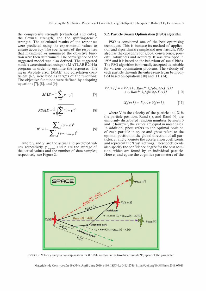
where y and y’ are the actual and predicted val-ues, respectively. y average and n are the average of the actual values and the number of data samples, respectively; see Figure 2.

5.2. Particle Swarm Optimisation (PSO) algorithm

PSO is considered one of the best optimising techniques. This is because its method of applica-tion and algorithm are simple and user-friendly. PSO also has the capability for global convergence, pow-erful robustness and accuracy. It was developed in 1995 and it is based on the behaviour of social birds. The PSO algorithm is normally accepted as suitable for various optimisation problems. The velocity of each particle through the entire search can be modi-fied based on equations [10] and [11] (34).

Vi(t+1] = wVi(t)+c1Rand(·)1[pbestit-Xi(t)]+c2 Rand(·)2[gbestit-Xi(t)] [10]

Xi(t+1) = Xi(t)+ Vi(t+1) [11]

where Vi is the velocity of the particle and Xi is the particle position. Rand (·)1 and Rand (·)2 are uniformly distributed random numbers between 0 and 1; however, the values are equal in most cases. In addition, pbest refers to the optimal position of each particle in space and gbest refers to the optimal position in the global direction of all par-ticles. c1 and c2 denote the acceleration coefficients and represent the ‘trust’ settings. These coefficients also specify the confidence degree for the best solu-tion, which are found by an individual particle. Here c1 and c2 are the cognitive parameters of the

Figure 2. Velocity and position explanation for the PSO method in the two dimensional (2D) space of the parameter

6 • H.H. Ghayeb et al.

Materiales de Construcción 69 (334), April–June 2019, e190. ISSN-L: 0465-2746. https://doi.org/10.3989/mc.2019.07018

entire swarm. w refers to the entire weight, and it is defined in a trial to upgrade the convergence pro-cess of the iteration. It is a scaling variable applied for controlling the abilities of the swarm’s explo-ration. It scales the current velocity, which affects the updating vector of velocity (35). The updat-ing position and particle velocity are depicted in Figure 2. The velocity contains three main vec-tors, as illustrated in Figure 2. The first vector is the internal component and momentum, which are based on the velocity of the particle’s previous time step. The memory or cognitive component is the second vector. It is a result of the iteration pro-cess on the best position of the particle. The third vector is the social component or swarm. The par-ticle in that element moves to the best position in the swarm.

5.3. Convergence criteria

The criteria of the convergence are to stop the optimisation process in order to calculate the optimum value of the objective function so as to evaluate the minimum error. Generally, the most and widely implemented criteria are the minimum error of the optimum value and the maximum iteration number of the algorithm of PSO. The reason for using a maximum number for the itera-tions can be related to the difficulties arising from the problem of the optimisation. Tables 2 and 3 presents the main parameters of PSO used in this study.

5.4. Implementing PSO with RSM

A total of the 47 mixtures were adopted to deter-mine the optimised equations required to evalu-ate the compressive, flexural and splitting-tensile strengths of the concrete. The conventional process of selecting parameters to enhance the mechani-cal properties of concrete involves substantial trial and error within the laboratory. Consequently, this process consumes time and increases the cost of producing concrete, due to the raw materials that the process requires. In addition, CO2 emissions will increase, due to the laboratory equipment used. Hence, a PSO algorithm is a more suitable method to determine the optimised parameters so as to improve the mechanical properties of normal concrete. The PSO algorithm can address issues related to a series of trial and error experiments in the laboratory. Accordingly, RSM performance can be enhanced. Thus, RSM and PSO algorithms can be combined to minimise error, referred to as the ‘hybrid PSO-RSM’ method. The PSO algo-rithm was implemented within MATLAB 2014a. The implementation of PSO is highlighted as fol-lows in order to define the optimum RSM of the concrete.

1. The swarm initialization is completed by the hyperspace task of each particle in its random position.

2. The proposed objective function of the RSM is evaluated for each particle.

3. The value of the objective function of each sep-arate particle is compared with its pbest. The pbest represents the best value from the comparison process. It can be the current pbest value or the value of the objective function.

4. The best value of the objective function of the particle is specified. The objective function value is evaluated to be gbest, and its position is gbest.

5. All particle positions and velocities are updated based on equations [10] and [11].

6. The target is the maximum number of iterations or when the suitability of the objective function is achieved through steps 2 to 5. The reparation process is continued until the target is achieved.

6. SPECIMEN MIXTURE DESIGN AND TESTING

Table 4 presents the mixture proportions of the concrete. Cylindrical samples of 300 mm in height

Table 2. The main parameters of PSO (36)

Parameter Description

Number of particles, N The best range is 10-40, but 50-100 is used for special or complex problems.

Particle dimensions It is defined based on the optimised problem.

Weight of inertia It is normally set to 0.70 for faster convergence, and w can be updated during the analysis.

The lower and upper constraints of the vectors of the n design

The values are defined based on the optimised problem. Generally, different ranges can be utilised.

Social and cognitive parameters

c1 = c2 = 1.494. In general, 0 < c1 + c2 < 4.

Table 3. The main parameters of algorithm of PSO (36)

Parameter Description

The maximum number of iterations for the termination criterion (Tmax)

Calculated from the optimised problem.

The number of iterations (kf) that is satisfied when checking for convergence

The objective function of the relative improvement divided by the last value of the number of iterations including the current iteration. It is less than or equal to fm.

The minimum objective function of the relative improvement (fm)

The relative improvement of the objective function over the last kf iteration (including the current iteration) is less or equal fm.

Predicting the Mechanical Properties of Concrete Using Intelligent Techniques to Reduce CO2 Emissions • 7

Materiales de Construcción 69 (334), April–June 2019, e190. ISSN-L: 0465-2746. https://doi.org/10.3989/mc.2019.07018

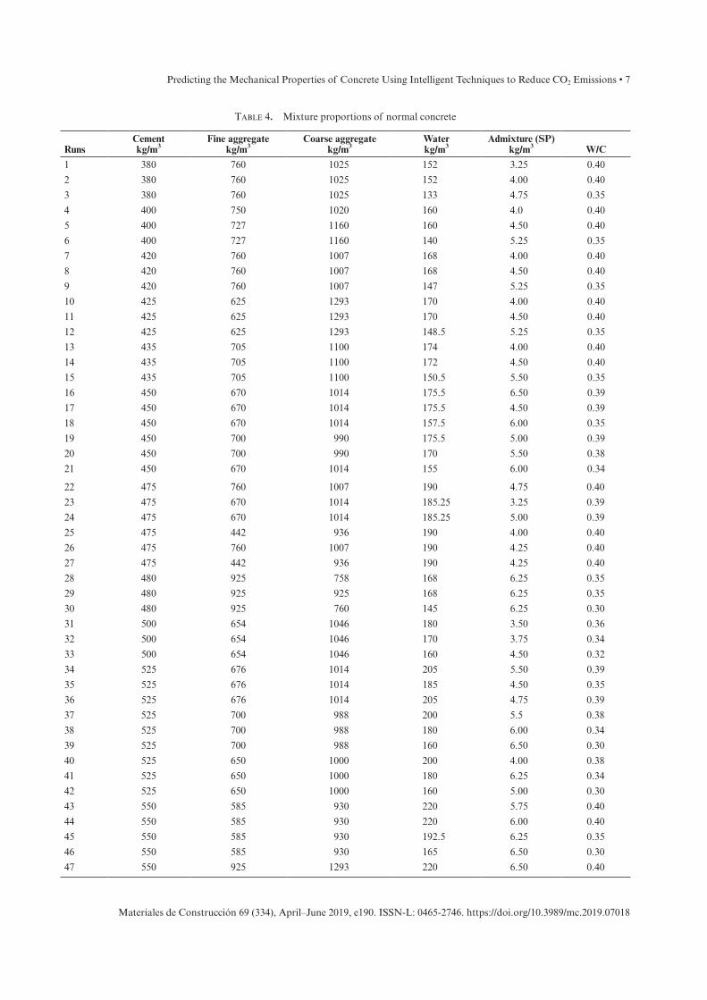
Table 4. Mixture proportions of normal concrete

RunsCementkg/m3

Fine aggregatekg/m3

Coarse aggregatekg/m3

Waterkg/m3

Admixture (SP)kg/m3 W/C

1 380 760 1025 152 3.25 0.40

2 380 760 1025 152 4.00 0.40

3 380 760 1025 133 4.75 0.35

4 400 750 1020 160 4.0 0.40

5 400 727 1160 160 4.50 0.40

6 400 727 1160 140 5.25 0.35

7 420 760 1007 168 4.00 0.40

8 420 760 1007 168 4.50 0.40

9 420 760 1007 147 5.25 0.35

10 425 625 1293 170 4.00 0.40

11 425 625 1293 170 4.50 0.40

12 425 625 1293 148.5 5.25 0.35

13 435 705 1100 174 4.00 0.40

14 435 705 1100 172 4.50 0.40

15 435 705 1100 150.5 5.50 0.35

16 450 670 1014 175.5 6.50 0.39

17 450 670 1014 175.5 4.50 0.39

18 450 670 1014 157.5 6.00 0.35

19 450 700 990 175.5 5.00 0.39

20 450 700 990 170 5.50 0.38

21 450 670 1014 155 6.00 0.34

22 475 760 1007 190 4.75 0.40

23 475 670 1014 185.25 3.25 0.39

24 475 670 1014 185.25 5.00 0.39

25 475 442 936 190 4.00 0.40

26 475 760 1007 190 4.25 0.40

27 475 442 936 190 4.25 0.40

28 480 925 758 168 6.25 0.35

29 480 925 925 168 6.25 0.35

30 480 925 760 145 6.25 0.30

31 500 654 1046 180 3.50 0.36

32 500 654 1046 170 3.75 0.34

33 500 654 1046 160 4.50 0.32

34 525 676 1014 205 5.50 0.39

35 525 676 1014 185 4.50 0.35

36 525 676 1014 205 4.75 0.39

37 525 700 988 200 5.5 0.38

38 525 700 988 180 6.00 0.34

39 525 700 988 160 6.50 0.30

40 525 650 1000 200 4.00 0.38

41 525 650 1000 180 6.25 0.34

42 525 650 1000 160 5.00 0.30

43 550 585 930 220 5.75 0.40

44 550 585 930 220 6.00 0.40

45 550 585 930 192.5 6.25 0.35

46 550 585 930 165 6.50 0.30

47 550 925 1293 220 6.50 0.40

8 • H.H. Ghayeb et al.

Materiales de Construcción 69 (334), April–June 2019, e190. ISSN-L: 0465-2746. https://doi.org/10.3989/mc.2019.07018

and 150 mm in diameter and cubes of 100 x 100 x 100 mm were stacked into three layers and compacted with vibration in compliance with the specifications of BS EN 12390-1 (2000) (37). Experimental tests were con-ducted after 28 days of curing the concrete samples in water. Compression tests were performed to com-ply with BS EN 12390-1, 3, and 4 (2009) (37, 38). In addition, flexural strength tests complied with BS EN 12390-5 (2009)(39) and splitting tensile strength tests complied with BS EN 12390-6 (2009)(40). The results reported were the average of three samples.

6.1. Experimental database of PSO and DOE methods

In this study, the experimental data of 47 mix-tures of concrete were utilised in the PSO and DOE methods. The input data of each run were collected as the amount of the constituent materials in each mixture, which were cement, fine aggregate, coarse aggregate, water, and SP. The number of runs was equal to the number of concrete mixtures; i.e. 47. The data sets available were divided randomly into learning, validation and testing subsets (36, 37). The training process in the PSO technique method was completed using the learning data. In addi-tion, the testing data were utilised to identify the

generalisation capacity of the models. The learn-ing and validation data were incorporated into the modelling process and were categorised into one set-group denoted as the training data. In most cases, it is recognised that the derived models utilising soft computing tools have a predictive ability within the data range used for development. Therefore, the quantity of data applied for the modelling process is a significant issue, as it affects the reliability of the final models (37). To address this issue, it was described the minimum ratio of the number of responses over the number of selected variables be three for model acceptability, though a value of five is safer (38). In the present study, this ratio was 7.6. Finally, 80% of the data was used to build the mod-els and 20% was used to verify the model’s accuracy.

7. RESULTS AND DISCUSSION OF THE DOE METHOD

7.1. Strength analysis

The compressive strength, flexural strength, and splitting-tensile strength were determined for the concrete samples. The failure of the samples occurred due to fracture of the coarse aggregate, as shown in Figure 3.

Figure 3. Failure mode of (a) compressive, (b) flexural, and (c) splitting tests

Predicting the Mechanical Properties of Concrete Using Intelligent Techniques to Reduce CO2 Emissions • 9

Materiales de Construcción 69 (334), April–June 2019, e190. ISSN-L: 0465-2746. https://doi.org/10.3989/mc.2019.07018

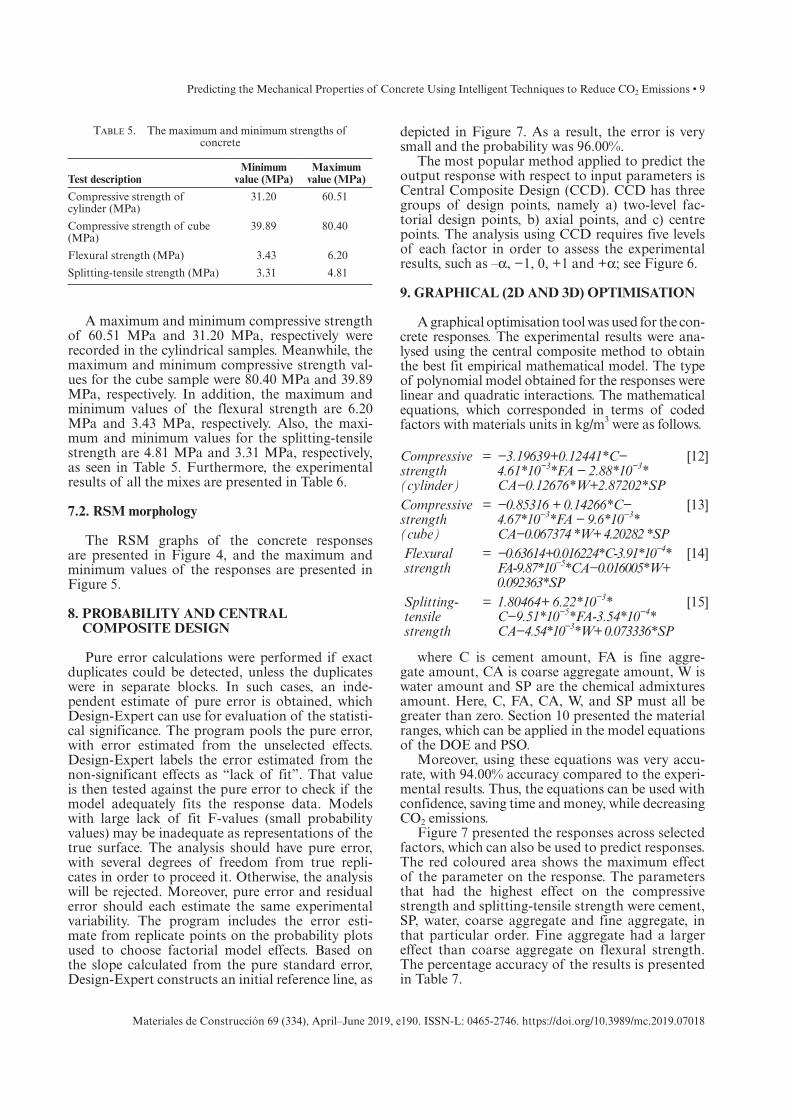
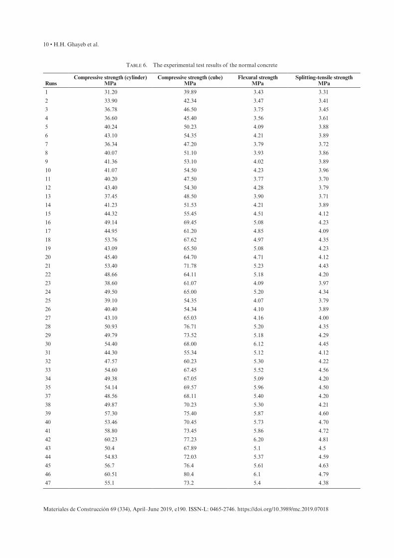
A maximum and minimum compressive strength of 60.51 MPa and 31.20 MPa, respectively were recorded in the cylindrical samples. Meanwhile, the maximum and minimum compressive strength val-ues for the cube sample were 80.40 MPa and 39.89 MPa, respectively. In addition, the maximum and minimum values of the flexural strength are 6.20 MPa and 3.43 MPa, respectively. Also, the maxi-mum and minimum values for the splitting-tensile strength are 4.81 MPa and 3.31 MPa, respectively, as seen in Table 5. Furthermore, the experimental results of all the mixes are presented in Table 6.

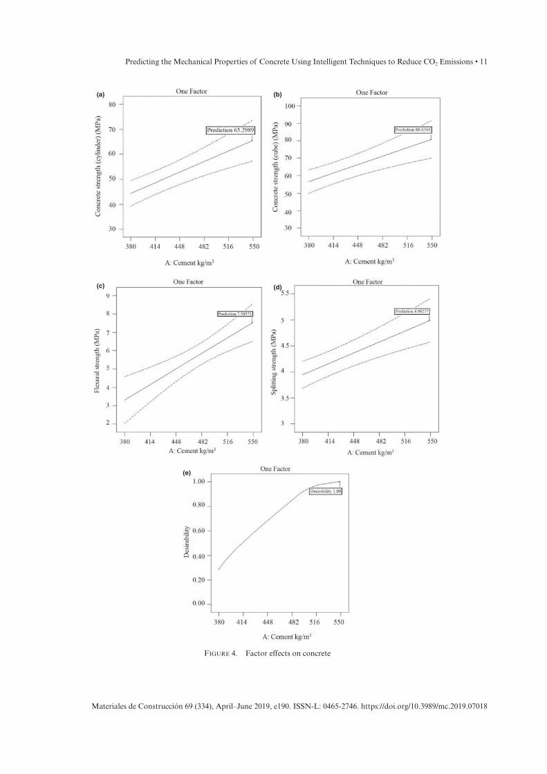
7.2. RSM morphology

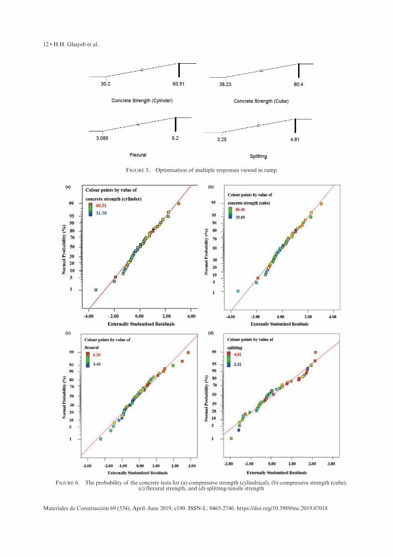
The RSM graphs of the concrete responses are presented in Figure 4, and the maximum and minimum values of the responses are presented in Figure 5.

8. PROBABILITY AND CENTRAL COMPOSITE DESIGN

Pure error calculations were performed if exact duplicates could be detected, unless the duplicates were in separate blocks. In such cases, an inde-pendent estimate of pure error is obtained, which Design-Expert can use for evaluation of the statisti-cal significance. The program pools the pure error, with error estimated from the unselected effects. Design-Expert labels the error estimated from the non-significant effects as “lack of fit”. That value is then tested against the pure error to check if the model adequately fits the response data. Models with large lack of fit F-values (small probability values) may be inadequate as representations of the true surface. The analysis should have pure error, with several degrees of freedom from true repli-cates in order to proceed it. Otherwise, the analysis will be rejected. Moreover, pure error and residual error should each estimate the same experimental variability. The program includes the error esti-mate from replicate points on the probability plots used to choose factorial model effects. Based on the slope calculated from the pure standard error, Design-Expert constructs an initial reference line, as

depicted in Figure 7. As a result, the error is very small and the probability was 96.00%.

The most popular method applied to predict the output response with respect to input parameters is Central Composite Design (CCD). CCD has three groups of design points, namely a) two-level fac-torial design points, b) axial points, and c) centre points. The analysis using CCD requires five levels of each factor in order to assess the experimental results, such as –a, −1, 0, +1 and +a; see Figure 6.

9. GRAPHICAL (2D AND 3D) OPTIMISATION

A graphical optimisation tool was used for the con-crete responses. The experimental results were ana-lysed using the central composite method to obtain the best fit empirical mathematical model. The type of polynomial model obtained for the responses were linear and quadratic interactions. The mathematical equations, which corresponded  in terms of coded factors with materials units in kg/m3 were as follows.

Compressive strength (cylinder)

= −3.19639+0.12441*C− 4.61*10−3*FA − 2.88*10−3* CA−0.12676*W+2.87202*SP

[12]

Compressive strength (cube)

= −0.85316 + 0.14266*C− 4.67*10−3*FA − 9.6*10−3* CA−0.067374 *W+ 4.20282 *SP

[13]

Flexural strength

= −0.63614+0.016224*C-3.91*10−4* FA-9.87*10−5*CA−0.016005*W+ 0.092363*SP

[14]

Splitting-tensile strength

= 1.80464+ 6.22*10−3* C−9.51*10−5*FA-3.54*10−4* CA−4.54*10−3*W+ 0.073336*SP

[15]

where C is cement amount, FA is fine aggre-gate amount, CA is coarse aggregate amount, W is water amount and SP are the chemical admixtures amount. Here, C, FA, CA, W, and SP must all be greater than zero. Section 10 presented the material ranges, which can be applied in the model equations of the DOE and PSO.

Moreover, using these equations was very accu-rate, with 94.00% accuracy compared to the experi-mental results. Thus, the equations can be used with confidence, saving time and money, while decreasing CO2 emissions.

Figure 7 presented the responses across selected factors, which can also be used to predict responses. The red coloured area shows the maximum effect of the parameter on the response. The parameters that had the highest effect on the compressive strength and splitting-tensile strength were cement, SP, water, coarse aggregate and fine aggregate, in that particular order. Fine aggregate had a larger effect than coarse aggregate on flexural strength. The percentage accuracy of the results is presented in Table 7.

Table 5. The maximum and minimum strengths of concrete

Test descriptionMinimum

value (MPa)Maximum

value (MPa)

Compressive strength of cylinder (MPa)

31.20 60.51

Compressive strength of cube (MPa)

39.89 80.40

Flexural strength (MPa) 3.43 6.20

Splitting-tensile strength (MPa) 3.31 4.81

10 • H.H. Ghayeb et al.

Materiales de Construcción 69 (334), April–June 2019, e190. ISSN-L: 0465-2746. https://doi.org/10.3989/mc.2019.07018

Table 6. The experimental test results of the normal concrete

RunsCompressive strength (cylinder)

MPaCompressive strength (cube)

MPaFlexural strength

MPaSplitting-tensile strength

MPa

1 31.20 39.89 3.43 3.31

2 33.90 42.34 3.47 3.41

3 36.78 46.50 3.75 3.45

4 36.60 45.40 3.56 3.61

5 40.24 50.23 4.09 3.88

6 43.10 54.35 4.21 3.89

7 36.34 47.20 3.79 3.72

8 40.07 51.10 3.93 3.86

9 41.36 53.10 4.02 3.89

10 41.07 54.50 4.23 3.96

11 40.20 47.50 3.77 3.70

12 43.40 54.30 4.28 3.79

13 37.45 48.50 3.90 3.71

14 41.23 51.53 4.21 3.89

15 44.32 55.45 4.51 4.12

16 49.14 69.45 5.08 4.23

17 44.95 61.20 4.85 4.09

18 53.76 67.62 4.97 4.35

19 43.09 65.50 5.08 4.23

20 45.40 64.70 4.71 4.12

21 53.40 71.78 5.23 4.43

22 48.66 64.11 5.18 4.20

23 38.60 61.07 4.09 3.97

24 49.50 65.00 5.20 4.34

25 39.10 54.35 4.07 3.79

26 40.40 54.34 4.10 3.89

27 43.10 65.03 4.16 4.00

28 50.93 76.71 5.20 4.35

29 49.79 73.52 5.18 4.29

30 54.40 68.00 6.12 4.45

31 44.30 55.34 5.12 4.12

32 47.57 60.23 5.30 4.22

33 54.60 67.45 5.52 4.56

34 49.38 67.05 5.09 4.20

35 54.14 69.57 5.96 4.50

37 48.56 68.11 5.40 4.20

38 49.87 70.23 5.30 4.21

39 57.30 75.40 5.87 4.60

40 53.46 70.45 5.73 4.70

41 58.80 73.45 5.86 4.72

42 60.23 77.23 6.20 4.81

43 50.4 67.89 5.1 4.5

44 54.83 72.03 5.37 4.59

45 56.7 76.4 5.61 4.63

46 60.51 80.4 6.1 4.79

47 55.1 73.2 5.4 4.38

Predicting the Mechanical Properties of Concrete Using Intelligent Techniques to Reduce CO2 Emissions • 11

Materiales de Construcción 69 (334), April–June 2019, e190. ISSN-L: 0465-2746. https://doi.org/10.3989/mc.2019.07018

Figure 4. Factor effects on concrete

(a)

(c) (d)

(e)

(b)

12 • H.H. Ghayeb et al.

Materiales de Construcción 69 (334), April–June 2019, e190. ISSN-L: 0465-2746. https://doi.org/10.3989/mc.2019.07018

Figure 5. Optimisation of multiple responses viewed in ramp

Figure 6. The probability of the concrete tests for (a) compressive strength (cylindrical), (b) compressive strength (cube), (c) flexural strength, and (d) splitting-tensile strength

(a)

(c) (d)

(b)

Predicting the Mechanical Properties of Concrete Using Intelligent Techniques to Reduce CO2 Emissions • 13

Materiales de Construcción 69 (334), April–June 2019, e190. ISSN-L: 0465-2746. https://doi.org/10.3989/mc.2019.07018

The accuracy of the results that used the equations, as presented in Table 7, revealed that the flexural strength, compressive strength, and splitting-tensile strength had slightly higher average values than the experimental results. The 3D surfaces of the responses are depicted in Figure 8. The response changed when other factors were added into each level, as shown in Figure 9. The figure also presents the effect of cement

and fine aggregate factors. Water and SP significantly influenced the result of the responses. The values of the response increased when the quantity of water decreased and quantity of SP increased. Additionally, the fine aggregate had a larger effect on controlling concrete paste strength than SP or coarse aggregate. Increasing the coarse aggregate quantity enhanced the splitting strength value.

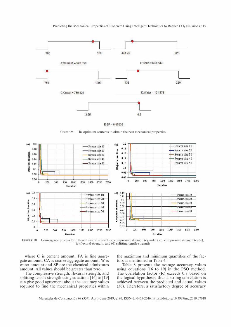
Based on the (2D) contour plots and (3D) sur-face responses, the results improved by increasing the quantities of cement, SP, coarse aggregate, and fine aggregate, as well as when decreasing the water ratio. The optimum contents of the concrete mix-ture in order to obtain the best mechanical proper-ties are presented in Figure 9.

10. RESULTS AND DISCUSSION OF THE PSO METHOD

Four PSO models were built to optimise the com-pressive, flexural, and splitting strengths of concrete. The parameters of these models represented the

Table 7. Analysis of result accuracy using the RSM method

Response item (MPa)

Range of experimental

results (MPa)

Range of equation

results (MPa)Accuracy

(%)

Compressive strength (cylinder)

31.20-60.51 33.60-62.96 94.91

Compressive strength (cube)

39.89-80.40 43.38-82.15 93.88

Flexural strength 3.43-6.20 3.59- 6.38 94.17

Splitting-tensile strength

3.31-4.81 3.42-4.68 95.68

Figure 7. The contour response graphs of the concrete analysis using the RSM method of (a) concrete strength (cylinder), (b) concrete strength (cube), (c) flexural strength, and (d) splitting strength

(a)

(c) (d)

(b)

14 • H.H. Ghayeb et al.

Materiales de Construcción 69 (334), April–June 2019, e190. ISSN-L: 0465-2746. https://doi.org/10.3989/mc.2019.07018

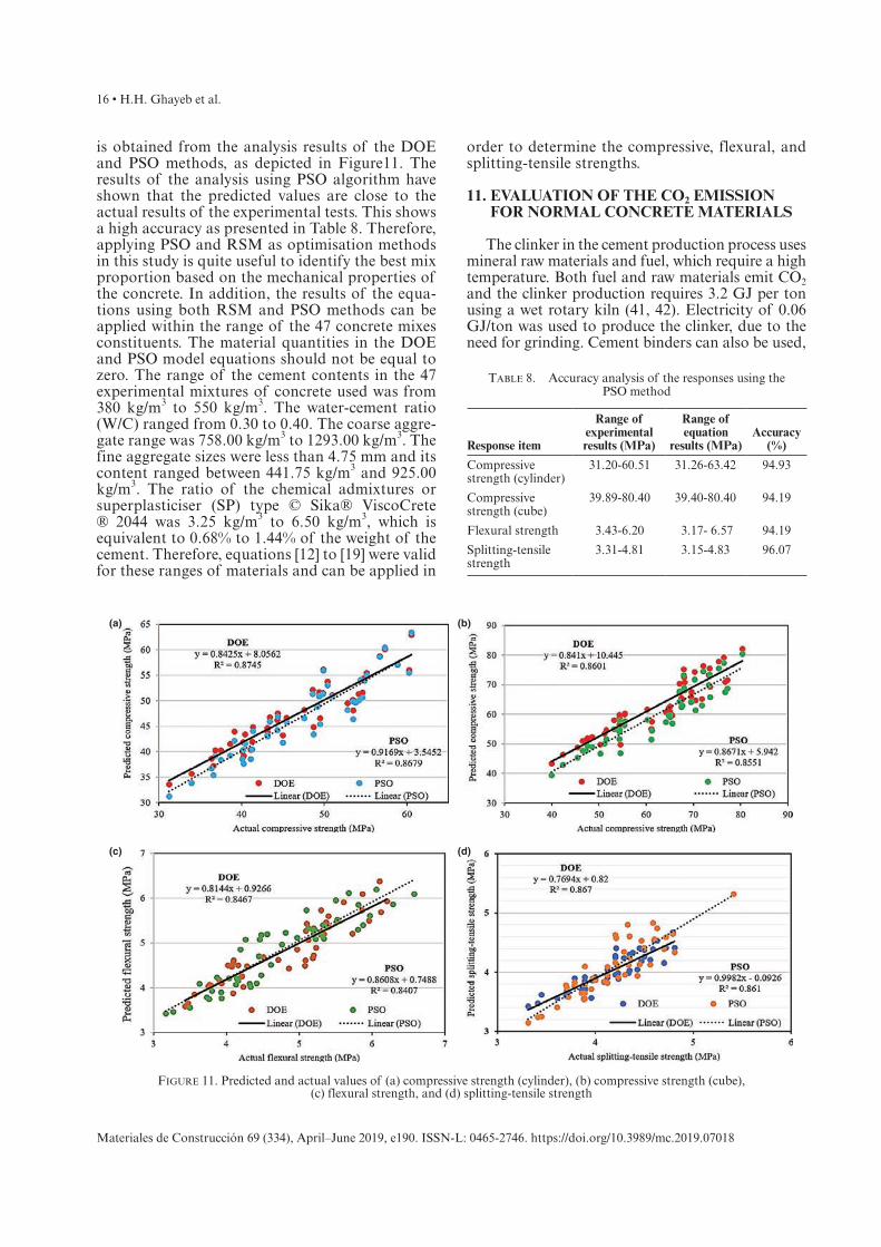
quantities of cement, water, SP, fine aggregate, and coarse aggregate. The target of the PSO objective func-tion was to minimise the variance of the predicted and measured strength. PSO provided the models to evalu-ate the strength capacity within the range of the maxi-mum and minimum quantities of the experimental results. The PSO algorithm was updated until a suit-able gbest was achieved or the maximum number of iter-ations was reached. The objective function variances were constant after 1200 iterations. Thus, the number of iterations was fixed at 2000, as depicted in Figure 10. In this study, 10, 20, 30, 40 and 50 particles were used to explore the effect of the number of particles on the accuracy of the models. The swarm sizes are presented in Figure 10, though 10, 20, 30, 40, and 50 were used for MAE to estimate the differences between the mea-sured and predicted mechanical properties of concrete. Figure 10 also shows the performance measure varia-tion values of the objective function for particles of different sizes. The best solution of the PSO algorithm

was provided by a swarm size of 40, as illustrated in Figure10. The remaining swarm sizes indicated higher errors and were more time consuming. Finally, equa-tions [16] to [19] presents the best factors to evaluate the mechanical properties of normal concrete.

Compressive strength (cylinder)

= -7.1682+ 0.1290*C- 4.93*10−3* FA-2.81* 10−3*CA-0.13930*W+3.52135*SP

[16]

Compressive strength (cube)

= -1.415279+ 0.13851*C -0.0103451*FA-0.0094932 *CA - 0.064522* W+ 4.7945*SP

[17]

Flexural strength

= -2.845105+ 0.020055* C- 6.64*10−4*FA- 5.82*10−4 *CA - 0.0207*W+ 0.1339*SP

[18]

Splitting-tensile strength

= -1.69745+ 0.007* C- 6.05*10−4* FA- 6.05*10−4 *CA- 4.50*10−3* W+ 0.1288*SP

[19]

Figure 8. Response surfaces in 3D for normal concrete using RSM analysis of (a) concrete strength (cylinder), (b) concrete strength (cube), (c) flexural strength, and (d) splitting strength

(a)

(c) (d)

(b)

Predicting the Mechanical Properties of Concrete Using Intelligent Techniques to Reduce CO2 Emissions • 15

Materiales de Construcción 69 (334), April–June 2019, e190. ISSN-L: 0465-2746. https://doi.org/10.3989/mc.2019.07018

where C is cement amount, FA is fine aggre-gate amount, CA is coarse aggregate amount, W is water amount and SP are the chemical admixtures amount. All values should be greater than zero.

The compressive strength, flexural strength, and splitting-tensile strength using equations [16] to [19] can give good agreement about the accuracy values required to find the mechanical properties within

the maximum and minimum quantities of the fac-tors as mentioned in Table 4.

Table 8 presents the average accuracy values using equations [16 to 19] in the PSO method. The correlation factor (R) exceeds 0.8 based on the logical hypothesis, thus a strong correlation is achieved between the predicted and actual values (36). Therefore, a satisfactory degree of accuracy

Figure 9. The optimum contents to obtain the best mechanical properties.

Figure 10. Convergence process for different swarm sizes of (a) compressive strength (cylinder), (b) compressive strength (cube), (c) flexural strength, and (d) splitting-tensile strength

(a)

(c) (d)

(b)

16 • H.H. Ghayeb et al.

Materiales de Construcción 69 (334), April–June 2019, e190. ISSN-L: 0465-2746. https://doi.org/10.3989/mc.2019.07018

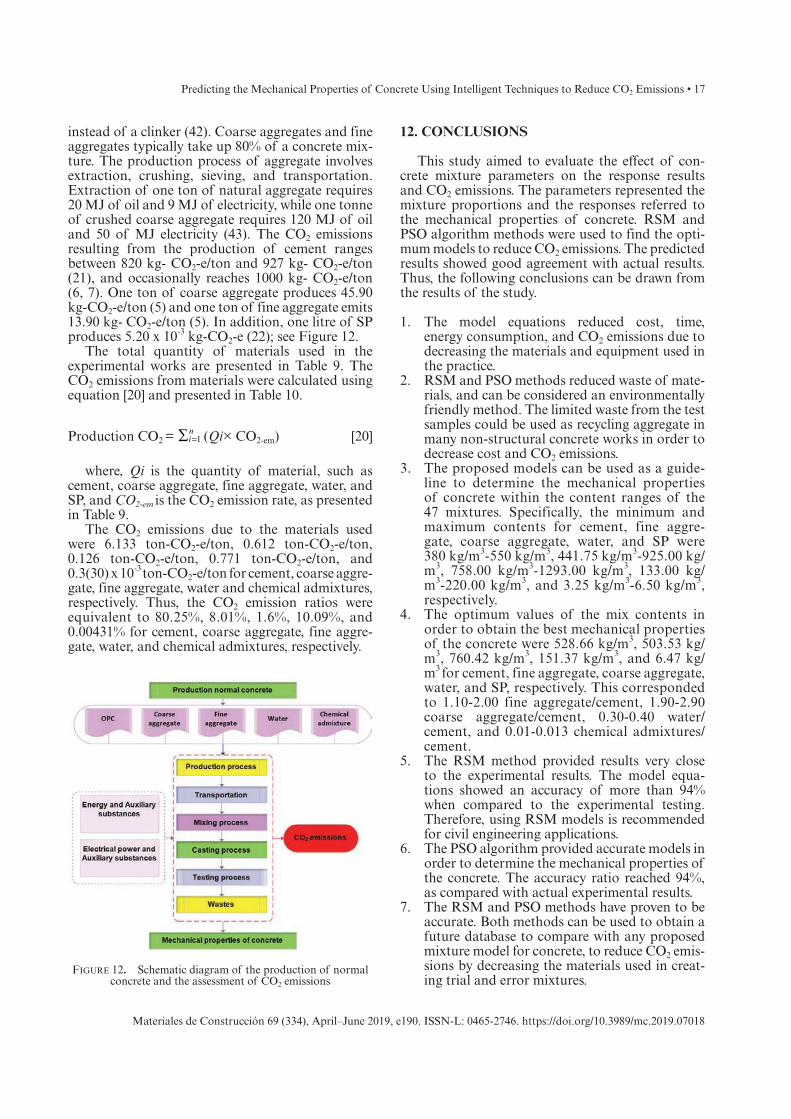
is obtained from the analysis results of the DOE and PSO methods, as depicted in Figure11. The results of the analysis using PSO algorithm have shown that the predicted values are close to the actual results of the experimental tests. This shows a high accuracy as presented in Table 8. Therefore, applying PSO and RSM as optimisation methods in this study is quite useful to identify the best mix proportion based on the mechanical properties of the concrete. In addition, the results of the equa-tions using both RSM and PSO methods can be applied within the range of the 47 concrete mixes constituents. The material quantities in the DOE and PSO model equations should not be equal to zero. The range of the cement contents in the 47 experimental mixtures of concrete used was from 380 kg/m3 to 550 kg/m3. The water-cement ratio (W/C) ranged from 0.30 to 0.40. The coarse aggre-gate range was 758.00 kg/m3 to 1293.00 kg/m3. The fine aggregate sizes were less than 4.75 mm and its content ranged between 441.75 kg/m3 and 925.00 kg/m3. The ratio of the chemical admixtures or superplasticiser (SP) type © Sika® ViscoCrete ® 2044 was 3.25 kg/m3 to 6.50 kg/m3, which is equivalent to 0.68% to 1.44% of the weight of the cement. Therefore, equations [12] to [19] were valid for these ranges of materials and can be applied in

order to determine the compressive, flexural, and splitting-tensile strengths.

11. EVALUATION OF THE CO2 EMISSION FOR NORMAL CONCRETE MATERIALS

The clinker in the cement production process uses mineral raw materials and fuel, which require a high temperature. Both fuel and raw materials emit CO2 and the clinker production requires 3.2 GJ per ton using a wet rotary kiln (41, 42). Electricity of 0.06 GJ/ton was used to produce the clinker, due to the need for grinding. Cement binders can also be used,

Figure 11. Predicted and actual values of (a) compressive strength (cylinder), (b) compressive strength (cube), (c) flexural strength, and (d) splitting-tensile strength

(a)

(c) (d)

(b)

Table 8. Accuracy analysis of the responses using the PSO method

Response item

Range of experimental results (MPa)

Range of equation

results (MPa)Accuracy

(%)

Compressive strength (cylinder)

31.20-60.51 31.26-63.42 94.93

Compressive strength (cube)

39.89-80.40 39.40-80.40 94.19

Flexural strength 3.43-6.20 3.17- 6.57 94.19

Splitting-tensile strength

3.31-4.81 3.15-4.83 96.07

Predicting the Mechanical Properties of Concrete Using Intelligent Techniques to Reduce CO2 Emissions • 17

Materiales de Construcción 69 (334), April–June 2019, e190. ISSN-L: 0465-2746. https://doi.org/10.3989/mc.2019.07018

instead of a clinker (42). Coarse aggregates and fine aggregates typically take up 80% of a concrete mix-ture. The production process of aggregate involves extraction, crushing, sieving, and transportation. Extraction of one ton of natural aggregate requires 20 MJ of oil and 9 MJ of electricity, while one tonne of crushed coarse aggregate requires 120 MJ of oil and 50 of MJ electricity (43). The CO2 emissions resulting from the production of cement ranges between 820 kg- CO2-e/ton and 927 kg- CO2-e/ton (21), and occasionally reaches 1000 kg- CO2-e/ton (6, 7). One ton of coarse aggregate produces 45.90 kg-CO2-e/ton (5) and one ton of fine aggregate emits 13.90 kg- CO2-e/ton (5). In addition, one litre of SP produces 5.20 x 10-3 kg-CO2-e (22); see Figure 12.

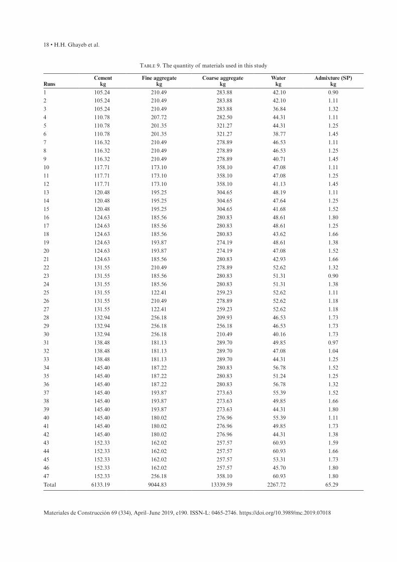
The total quantity of materials used in the experimental works are presented in Table 9. The CO2 emissions from materials were calculated using equation [20] and presented in Table 10.

Production CO2 = in

1∑ = (Qi× CO2-em) [20]

where, Qi is the quantity of material, such as cement, coarse aggregate, fine aggregate, water, and SP, and CO2-em is the CO2 emission rate, as presented in Table 9.

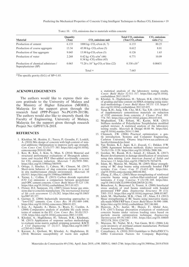
The CO2 emissions due to the materials used were 6.133 ton-CO2-e/ton, 0.612 ton-CO2-e/ton, 0.126 ton-CO2-e/ton, 0.771 ton-CO2-e/ton, and 0.3(30) x 10-3 ton-CO2-e/ton for cement, coarse aggre-gate, fine aggregate, water and chemical admixtures, respectively. Thus, the CO2 emission ratios were equivalent to 80.25%, 8.01%, 1.6%, 10.09%, and 0.00431% for cement, coarse aggregate, fine aggre-gate, water, and chemical admixtures, respectively.

12. CONCLUSIONS

This study aimed to evaluate the effect of con-crete mixture parameters on the response results and CO2 emissions. The parameters represented the mixture proportions and the responses referred to the mechanical properties of concrete. RSM and PSO algorithm methods were used to find the opti-mum models to reduce CO2 emissions. The predicted results showed good agreement with actual results. Thus, the following conclusions can be drawn from the results of the study.

1. The model equations reduced cost, time, energy consumption, and CO2 emissions due to decreasing the materials and equipment used in the practice.

2. RSM and PSO methods reduced waste of mate-rials, and can be considered an environmentally friendly method. The limited waste from the test samples could be used as recycling aggregate in many non-structural concrete works in order to decrease cost and CO2 emissions.

3. The proposed models can be used as a guide-line to determine the mechanical properties of concrete within the content ranges of the 47 mixtures. Specifically, the minimum and maximum contents for cement, fine aggre-gate, coarse aggregate, water, and SP were 380 kg/m3-550 kg/m3, 441.75 kg/m3-925.00 kg/m3, 758.00 kg/m3-1293.00 kg/m3, 133.00 kg/m3-220.00 kg/m3, and 3.25 kg/m3-6.50 kg/m3, respectively.

4. The optimum values of the mix contents in order to obtain the best mechanical properties of the concrete were 528.66 kg/m3, 503.53 kg/m3, 760.42 kg/m3, 151.37 kg/m3, and 6.47 kg/m3 for cement, fine aggregate, coarse aggregate, water, and SP, respectively. This corresponded to 1.10-2.00 fine aggregate/cement, 1.90-2.90 coarse aggregate/cement, 0.30-0.40 water/cement, and 0.01-0.013 chemical admixtures/cement.

5. The RSM method provided results very close to the experimental results. The model equa-tions showed an accuracy of more than 94% when compared to the experimental testing. Therefore, using RSM models is recommended for civil engineering applications.

6. The PSO algorithm provided accurate models in order to determine the mechanical properties of the concrete. The accuracy ratio reached 94%, as compared with actual experimental results.

7. The RSM and PSO methods have proven to be accurate. Both methods can be used to obtain a future database to compare with any proposed mixture model for concrete, to reduce CO2 emis-sions by decreasing the materials used in creat-ing trial and error mixtures.

Figure 12. Schematic diagram of the production of normal concrete and the assessment of CO2 emissions

18 • H.H. Ghayeb et al.

Materiales de Construcción 69 (334), April–June 2019, e190. ISSN-L: 0465-2746. https://doi.org/10.3989/mc.2019.07018

Table 9. The quantity of materials used in this study

RunsCement

kgFine aggregate

kgCoarse aggregate

kgWater

kgAdmixture (SP)

kg1 105.24 210.49 283.88 42.10 0.902 105.24 210.49 283.88 42.10 1.11

3 105.24 210.49 283.88 36.84 1.32

4 110.78 207.72 282.50 44.31 1.11

5 110.78 201.35 321.27 44.31 1.25

6 110.78 201.35 321.27 38.77 1.45

7 116.32 210.49 278.89 46.53 1.11

8 116.32 210.49 278.89 46.53 1.25

9 116.32 210.49 278.89 40.71 1.45

10 117.71 173.10 358.10 47.08 1.11

11 117.71 173.10 358.10 47.08 1.25

12 117.71 173.10 358.10 41.13 1.45

13 120.48 195.25 304.65 48.19 1.11

14 120.48 195.25 304.65 47.64 1.25

15 120.48 195.25 304.65 41.68 1.52

16 124.63 185.56 280.83 48.61 1.80

17 124.63 185.56 280.83 48.61 1.25

18 124.63 185.56 280.83 43.62 1.66

19 124.63 193.87 274.19 48.61 1.38

20 124.63 193.87 274.19 47.08 1.52

21 124.63 185.56 280.83 42.93 1.66

22 131.55 210.49 278.89 52.62 1.32

23 131.55 185.56 280.83 51.31 0.90

24 131.55 185.56 280.83 51.31 1.38

25 131.55 122.41 259.23 52.62 1.11

26 131.55 210.49 278.89 52.62 1.18

27 131.55 122.41 259.23 52.62 1.18

28 132.94 256.18 209.93 46.53 1.73

29 132.94 256.18 256.18 46.53 1.73

30 132.94 256.18 210.49 40.16 1.73

31 138.48 181.13 289.70 49.85 0.97

32 138.48 181.13 289.70 47.08 1.04

33 138.48 181.13 289.70 44.31 1.25

34 145.40 187.22 280.83 56.78 1.52

35 145.40 187.22 280.83 51.24 1.25

36 145.40 187.22 280.83 56.78 1.32

37 145.40 193.87 273.63 55.39 1.52

38 145.40 193.87 273.63 49.85 1.66

39 145.40 193.87 273.63 44.31 1.80

40 145.40 180.02 276.96 55.39 1.11

41 145.40 180.02 276.96 49.85 1.73

42 145.40 180.02 276.96 44.31 1.38

43 152.33 162.02 257.57 60.93 1.59

44 152.33 162.02 257.57 60.93 1.66

45 152.33 162.02 257.57 53.31 1.73

46 152.33 162.02 257.57 45.70 1.80

47 152.33 256.18 358.10 60.93 1.80

Total 6133.19 9044.83 13339.59 2267.72 65.29

Predicting the Mechanical Properties of Concrete Using Intelligent Techniques to Reduce CO2 Emissions • 19

Materiales de Construcción 69 (334), April–June 2019, e190. ISSN-L: 0465-2746. https://doi.org/10.3989/mc.2019.07018

ACKNOWLEDGEMENTS

The authors would like to express their sin-cere gratitude to the University of Malaya and the Ministry of Higher Education (MOHE), Malaysia for the support given through the research fund (PPP-Project No.PG199-2015B). The authors would also like to sincerely thank the Faculty of Engineering, University of Malaya, Malaysia for the support given through research Project No: GPF071A-2018.

REFERENCES

1. Khokhar, M.; Rozière, E.; Turcry, P.; Grondin, F.; Loukili, A. (2010) Mix design of concrete with high content of min-eral additions: Optimisation to improve early age strength. Cem. Concr. Com. 32 (5):377–385. https://doi.org/10.1016/j.cemconcomp.2010.01.006.

2. Koo, B.; Kim, J.; Kim, S.; Mun, S. (2014) Material and structural performance evaluations of Hwangtoh admix-tures and recycled PET fiber-added eco-friendly concrete for CO2 emission reduction. Materials 7 (8):5959–5981. https://doi.org/10.3390/ma7085959.

3. Ortega, J.; Sánchez, I.; Cabeza, M.; Climent, M. (2017) Short-term behavior of slag concretes exposed to a real in situ mediterranean climate environment. Materials 10 (8):915. https://doi.org/10.3390/ma10080915.

4. Turner, L.; Collins, F. (2013) Carbon dioxide equivalent (CO 2-e) emissions: a comparison between geopolymer and OPC cement concrete. Constr. Build Mater 43:125–130. https://doi.org/10.1016/j.conbuildmat.2013.01.023.

5. Flower, D.J.; Sanjayan, J.G. (2007) Green house gas emis-sions due to concrete manufacture. The international Journal of life cycle assessment 12 (5):282. https://doi.org/10.1065/lca2007.05.327.

6. Gartner, E. (2004) Industrially interesting approaches to “low-CO2” cements. Cem. Concr. Res. 34 (9):1489–1498. https://doi.org/10.1016/j.cemconres.2004.01.021.

7. Josa, A.; Aguado, A.; Heino, A.; Byars, E.; Cardim, A. (2004) Comparative analysis of available life cycle inven-tories of cement in the EU. Cem. Concr. Res. 34 (8):1313–1320. https://doi.org/10.1016/j.cemconres.2003.12.020.

8. Khodaii, A.; Haghshenas, H.; Tehrani, H.K.; Khedmati, M. (2013) Application of response surface methodology to evaluate stone matrix asphalt stripping potential. KSCE J. Civil Engineering 17 (1):117. https://doi.org/10.1007/s12205-013-1698-6.

9. Kavussi, A.; Qorbani, M.; Khodaii, A.; Haghshenas,  H. (2014) Moisture susceptibility of warm mix asphalt:

a statistical analysis of the laboratory testing results. Constr. Build Mater 52:511–517. https://doi.org/10.1016/j.conbuildmat.2013.10.073.

10. Khodaii, A.; Haghshenas, H.; Tehrani, H.K. (2012) Effect of grading and lime content on HMA stripping using statis-tical methodology. Constr. Build Mater 34:131–135. https://doi.org/10.1016/j.conbuildmat.2012.02.025.

11. Yang, K.H.; Jung, Y.B.; Cho, M.S.; Tae, S.H. (2015) Effect of supplementary cementitious materials on reduction of  CO2 emissions from concrete. J. Cleaner Prod. 103: 774–783. https://doi.org/10.1016/j.jclepro.2014.03.018.

12. Moghaddam, T.B.; Soltani, M.; Karim, M.R. (2015) Stiffness modulus of Polyethylene Terephthalate modified asphalt mixture: A statistical analysis of the laboratory testing results. Materials & Design 68:88–96. https://doi.org/10.1016/j.matdes.2014.11.044.

13. Chinneck, J.W. (2006) Practical optimization: a gen-tle introduction. Systems and Computer Engineering, Carleton University, Ottawa http://www.sce.carleton.ca/faculty/chinneck/po.html.

14. Van Stralen, K.J.; Jager, K.J.; Zoccali, C.; Dekker, F.W. (2008) Agreement between methods. Kidney international 74 (9):1116–1120. https://doi.org/10.1038/ki.2008.306.

15. Gordan, M.; Razak, H.A.; Ismail, Z.; Ghaedi, K. (2017) Recent developments in damage identification of structures using data mining. Latin American Journal of Solids and Structures 13. https://doi.org/10.1590/1679-78254378.

16. Islam, M.; Mansur, M.; Maalej, M. (2005) Shear strength-ening of RC deep beams using externally bonded FRP systems. Cem. Concr. Com 27 (3):413–420. https://doi.org/10.1016/j.cemconcomp.2004.04.002.

17. Zhang, Z.; Hsu, C. (2005) Shear strengthening of reinforced concrete beams using carbon-fiber-reinforced polymer laminates. J. Comp. Construc. 9 (2):158–169. https://doi.org/10.1061/(ASCE)1090-0268(2005)9:2(158).

18. Benachour, A.; Benyoucef, S.; Tounsi, A. (2008) Interfacial stress analysis of steel beams reinforced with bonded prestressed FRP plate. Engineering Structures 30 (11): 3305–3315. https://doi.org/10.1016/j.engstruct.2008.05.007.

19. Jalali, M.; Sharbatdar, M.K.; Chen, J.F.; Alaee, F.J. (2012) Shear strengthening of RC beams using innovative manu-ally made NSM FRP bars. Constr. Build Mater 36: 990–1000. https://doi.org/10.1016/j.conbuildmat.2012.06.068.

20. Hanoon, A.N.; Jaafar, M.; Hejazi, F.; Abdul Aziz, F.N. (2017) Energy absorption evaluation of reinforced concrete beams under various loading rates based on particle swarm optimization technique. Engineering Optimization 49 (9):1483–1501. https://doi.org/10.1080/0305215X.2016.1256729.

21. Marceau, M.; Nisbet, M.A.; Van Geem, M.G. (2006) Life cycle inventory of portland cement manufacture. Portland Cement Association, Illinois.

22. Consultancy, A. (2010) 2010 Guidelines to Defra/DECC\’s GHG Conversion Factors for Company Reporting;

Table 10. CO2 emissions due to materials within concrete

Material Quantity

(Ton) CO2 emissions unitTotal CO2 emissions

(Ton-CO2-e/ton)CO2 emissions

ratio (%)

Production of cement 6.133 1000 kg- CO2-e/ton (6, 7) 6.133 80.25

Production of coarse aggregate 13.34 45.90 kg- CO2-e/ton (5) 0.612 8.01

Production of fine aggregate 9.045 13.90 kg-CO2-e/ton (5) 0.126 1.65

Production of water 2.268 0.42 kg -CO2-e/m3 (44)0.34 kg -CO2-e/litre (45)

0.771 10.09

Production of chemical admixture /Superplasticiser (SP)

0.065 *5.20 x 10-3 kg-CO2-e/ litre (22) 0.330 x10-3 0.00431

Total = 7.643

*The specific gravity (S.G.) of SP=1.03.

20 • H.H. Ghayeb et al.

Materiales de Construcción 69 (334), April–June 2019, e190. ISSN-L: 0465-2746. https://doi.org/10.3989/mc.2019.07018

produced by AEA for the Department of Energy and Climate Change (DECC) and the Department for Environment, Food and Rural Affairs (Defra), Version 1.2. 1; download at http://archive.defra.gov.uk/environment/business/reporting/conversion-factors.htm; also available in Excel file format; last accessed June 2012.

23. ASTM-C192 (2003) Standard Practice for Making and Curing Concrete Test Specimens in the Laboratory Annual Book of ASTM Standards 4.02. ASTM International, West Conshohocken, PA.

24. Khuri, A.I.; John, A. (1996) Cornell, Response Surfaces, Designs and Analyses, Revised and Expanded [edition], Chapter 2, Matrix Algebra, Least Squares, the Analysis of Variance, and Principles of Experimental Design. Marcel Dekker, Inc., New York.

25. Myers, R.H.; Montgomery, D.C.; Vining, G.G.; Borror, C.M.; Kowalski, S.M. (2004) Response surface methodol-ogy: a retrospective and literature survey. J. quality technol-ogy 36 (1):53. https://doi.org/10.1080/00224065.2004.11980252.

26. Azargohar, R.; Dalai, A. (2005) Production of activated carbon from Luscar char: experimental and modeling stud-ies. Microporous and mesoporous materials 85 (3):219–225. https://doi.org/10.1016/j.micromeso.2005.06.018.

27. Pouran, S.R. Aziz, A.A.; Daud, W.; Shamshirband, S. (2015) Estimation of the effect of catalyst physical characteristics on Fenton-like oxidation efficiency using adaptive neuro-fuzzy computing technique. Measurement 59:314–328.

28. Moghaddam, T.B.; Soltani, M.; Karim, M.R.; Baaj, H. (2015) Optimization of asphalt and modifier contents for polyethylene terephthalate modified asphalt mixtures using response surface methodology. Measurement 74:159–169. https://doi.org/10.1016/j.measurement.2015.07.012.

29. Soltani, M.; Moghaddam, T.B.; Karim, M.R.; Baaj,  H. (2015) Analysis of fatigue properties of unmodified and polyethylene terephthalate modified asphalt mix-tures using response surface methodology.Engineering Failure Analysis 58:238–248. https://doi.org/10.1016/j.engfailanal.2015.09.005.

30. Pourtahmasb, M.S.; Karim, M.R.; Shamshirband, S. (2015) Resilient modulus prediction of asphalt mixtures containing recycled concrete aggregate using an adaptive neuro-fuzzy methodology. Constr. Build Mater 82:257–263. https://doi.org/10.1016/j.conbuildmat.2015.02.030.

31. Can, M.Y.; Kaya, Y.; Algur, O.F. (2006) Response sur-face optimization of the removal of nickel from aqueous solution by cone biomass of Pinus sylvestris. Bioresource technology 97 (14):1761–1765. https://doi.org/10.1016/j.biortech.2005.07.017.

32. Aksu, Z.; Gönen, F. (2006) Binary biosorption of phenol and chromium (VI) onto immobilized activated sludge in a packed bed: prediction of kinetic parameters and break-through curves. Separation and Purification Technology 49 (3):205–216. https://doi.org/10.1016/j.seppur.2005.09.014.

33. Körbahti, B.K.; Rauf, M.A. (2009) Determination of opti-mum operating conditions of carmine decoloration by UV/H 2 O 2 using response surface methodology. J. haz-ardous materials 161 (1):281–286. https://doi.org/10.1016/j.jhazmat.2008.03.118.

34. Kulkarni, R.V.; Venayagamoorthy, G.K. (2011) Particle swarm optimization in wireless-sensor networks: A brief sur-vey. IEEE Transactions on Systems, Man, and Cybernetics, Part C (Applications and Reviews) 41 (2):262–267. https://doi.org/10.1109/TSMCC.2010.2054080.

35. Eberhart, R.; Kennedy, J. (1995) A new optimizer using particle swarm theory. In: Micro Machine and Human Science. MHS’95., Proceedings of the Sixth International Symposium on, 1995. IEEE, pp 39–43. https://doi.org/10.1109/MHS.1995.494215.

36. Hanoon, A.N.; Jaafar, M.; Hejazi, F.; Aziz, F.N. (2017) Strut-and-tie model for externally bonded CFRP-strengthened reinforced concrete deep beams based on particle swarm optimization algorithm: CFRP debonding and rupture. Constr. Build Mater 147:428–447. https://doi.org/10.1016/j.conbuildmat.2017.04.094.

37. EN, B. (2000) 12390-1 Testing hardened concrete–Part 1: Shape, dimensions and other requirements for specimens and moulds. European Committee for Standardization.

38. EN, B. (2009) 12390-3 (2009) Testing hardened concrete—part 3: compressive strength of test specimens. British Standards Institution.

39. EN, B. (2009) 12390-5. Testing hardened concrete–Part 5: flexural strength of test specimens. British Standards Institution-BSI and CEN European Committee for Standardization.

40. EN, B. (2009) 12390-6 2009 Testing hardened concrete, Part 6: tensile splitting strength of test specimens. British Standards Institution.

41. Worrell, E.; Price, L.; Martin, N.; Hendriks, C.; Meida, L.O. (2001) Carbon dioxide emissions from the global cement industry. Annual review of energy and the envi-ronment 26 (1):303–329. https://doi.org/10.1146/annurev.energy.26.1.303.

42. Gustavsson, L.; Sathre, R. (2006) Variability in energy and carbon dioxide balances of wood and concrete building materials. Building and Environment 41 (7):940–951. https://doi.org/10.1016/j.buildenv.2005.04.008.

43. Worrell, E.; Van Heijningen, R.; De Castro, J.; Hazewinkel, J.; De Beer, J.; Faaij, A.; Vringer, K. (1994) New gross energy-requirement figures for materials production. Energy 19 (6):627–640. https://doi.org/10.1016/0360-5442(94)90003-5.

44. Hong, J.; Shen, G.Q.; Feng, Y.; Lau, W.S.; Mao, C. (2015) Greenhouse gas emissions during the construction phase of a building: a case study in China. J. Cleaner Production 103:249–259. https://doi.org/10.1016/j.jclepro.2014.11.023.

45. DECC (2011) 2011 guidelines to DEFRA/DECC’s GHG conversion factors for company reporting: Methodology paper for emission factors.