predicting taxi passenger demand using artificial neural...
TRANSCRIPT

IN DEGREE PROJECT COMPUTER SCIENCE AND ENGINEERING,SECOND CYCLE, 30 CREDITS
, STOCKHOLM SWEDEN 2017
Predicting taxi passenger demand using artificial neural networks
GUSTAV ZANDER
KTH ROYAL INSTITUTE OF TECHNOLOGYSCHOOL OF COMPUTER SCIENCE AND COMMUNICATION

Predicting taxi passenger demand using artificialneural networks
GUSTAV ZANDER
Master’s Thesis at NADASupervisor: Jeanette Hellgren Kotaleski
Examiner: Johan Håstad


Abstract
In this report a machine learning method using artificialneural networks to estimate taxi demand in di�erent geo-graphical zones in the city of Stockholm is proposed. Anattempt to determine the most important input featuresthat a�ect taxi ridership is performed and a network archi-tecture is conceived and trained using taxi ridership datafrom a major taxi company operating in the city. The re-sults show that except for the two basic input parameters,the hour of the day and the zone, the day of the week isclearly the most important factor. Also days after pay-ment and month of the year seems to be mildly relevantfactors while rain and temperature hardly a�ect the resultsat all. The final network model conceived was capable ofestimating taxi demand in Stockholm with an average errorof 2.73 rides and a success rate of 46 % of the rides using aboundary of 30 % or 1 ride.

Referat
Uppskattning av taxibeställningar med
artificiella neurala nätverk
I den här rapporten utvecklas och utvärderas en metod föratt uppskatta taxibehov i olika geografiska zoner i Stock-holm med hjälp av artificiella neurala nätverk. Rapportenfokuserar på att ta reda på de mest relevanta parametrar-na som påverkar taxiåkande. Dessa används som indata tillett neuralt nätverk som tränas med historisk data från ettav Stockholms största taxibolag. Resultaten visar hur vissaparametrar såsom timme på dygnet samt veckodag tydligtpåverkar mängden taxiresor i olika områden medan andraparametrar såsom temperatur och nederbörd knappt på-verkar taxiresande alls. Det slutliga valet av modell och in-putparametrar lyckas förutspå korrekt antal körningar medett snittfel på 2.73 körningar eller i 46 % av fallen i testda-tan när man räknar en korrekt uppskattning att ligga sommest 30 % eller en körning ifrån det korrekta värdet.

Contents
1 Introduction 21.1 Purpose and goals . . . . . . . . . . . . . . . . . . . . . . . . . . . . 31.2 Delimitations . . . . . . . . . . . . . . . . . . . . . . . . . . . . . . . 3
2 Background 52.1 Machine learning . . . . . . . . . . . . . . . . . . . . . . . . . . . . . 52.2 Supervised learning . . . . . . . . . . . . . . . . . . . . . . . . . . . . 52.3 Artificial neural networks . . . . . . . . . . . . . . . . . . . . . . . . 62.4 Implementation of artificial neural networks . . . . . . . . . . . . . . 8
2.4.1 Architecture . . . . . . . . . . . . . . . . . . . . . . . . . . . 92.4.2 Activation functions . . . . . . . . . . . . . . . . . . . . . . . 102.4.3 Learning . . . . . . . . . . . . . . . . . . . . . . . . . . . . . . 122.4.4 Input parameters . . . . . . . . . . . . . . . . . . . . . . . . . 132.4.5 Error and validation . . . . . . . . . . . . . . . . . . . . . . . 142.4.6 Cross-validation . . . . . . . . . . . . . . . . . . . . . . . . . 16
2.5 Related work . . . . . . . . . . . . . . . . . . . . . . . . . . . . . . . 16
3 Method and experiment 183.1 Data . . . . . . . . . . . . . . . . . . . . . . . . . . . . . . . . . . . . 18
3.1.1 Implementation . . . . . . . . . . . . . . . . . . . . . . . . . . 203.2 Optimizing the network . . . . . . . . . . . . . . . . . . . . . . . . . 21
3.2.1 Metrics for network optimization . . . . . . . . . . . . . . . . 213.2.2 Loss function . . . . . . . . . . . . . . . . . . . . . . . . . . . 213.2.3 Architecture . . . . . . . . . . . . . . . . . . . . . . . . . . . 22
3.3 Input parameter experimentation . . . . . . . . . . . . . . . . . . . . 233.3.1 Validation technique . . . . . . . . . . . . . . . . . . . . . . . 263.3.2 Baseline . . . . . . . . . . . . . . . . . . . . . . . . . . . . . . 263.3.3 Metrics for feature testing and final network validation . . . . 263.3.4 Final testing . . . . . . . . . . . . . . . . . . . . . . . . . . . 27
4 Results 284.1 Architecture evaluation . . . . . . . . . . . . . . . . . . . . . . . . . 28
4.1.1 Hidden neurons . . . . . . . . . . . . . . . . . . . . . . . . . . 28

4.1.2 Hidden layers . . . . . . . . . . . . . . . . . . . . . . . . . . . 294.1.3 Optimization algorithm . . . . . . . . . . . . . . . . . . . . . 304.1.4 Activation function . . . . . . . . . . . . . . . . . . . . . . . . 314.1.5 Overfitting . . . . . . . . . . . . . . . . . . . . . . . . . . . . 334.1.6 Final network implementation parameters . . . . . . . . . . . 35
4.2 Feature set evaluation . . . . . . . . . . . . . . . . . . . . . . . . . . 354.2.1 Prediction result plots from chronological validation . . . . . 36
4.3 Performance of final network model . . . . . . . . . . . . . . . . . . . 404.3.1 Comparison of results using di�erent thresholds . . . . . . . . 41
4.4 Di�erent encoding experiment . . . . . . . . . . . . . . . . . . . . . . 41
5 Discussion and Conclusions 435.1 Loss function convergence . . . . . . . . . . . . . . . . . . . . . . . . 435.2 Input variable encoding . . . . . . . . . . . . . . . . . . . . . . . . . 435.3 Feature sets . . . . . . . . . . . . . . . . . . . . . . . . . . . . . . . . 445.4 Network performance . . . . . . . . . . . . . . . . . . . . . . . . . . . 455.5 Evaluation metrics . . . . . . . . . . . . . . . . . . . . . . . . . . . . 455.6 Best results . . . . . . . . . . . . . . . . . . . . . . . . . . . . . . . . 465.7 Conclusions . . . . . . . . . . . . . . . . . . . . . . . . . . . . . . . . 465.8 Future work . . . . . . . . . . . . . . . . . . . . . . . . . . . . . . . . 47
5.8.1 Classification model . . . . . . . . . . . . . . . . . . . . . . . 475.8.2 Further parameter evaluation . . . . . . . . . . . . . . . . . . 47
Bibliography 49

CONTENTS
Glossary• ANN, short for Artificial neural network
• Epoch, A full round of training over the whole dataset
• Loss function, the function describing how much loss the network predictionshave, namely how much o� from a perfect prediction the network is.
• Cost, Other term commonly used to denote loss
1

Chapter 1
Introduction
Taxi services are a central transportation method in almost all urban areas. Likeso many other fields today the taxi business is undergoing a rapid digital trans-formation with new actors like Uber taking market shares with innovative digitalproducts.
The most important objective for any taxi company and driver is to minimizethe vacant driving time, and a very important aspect of this is to know where tofind the passengers. Naturally, we can never know where the passengers will be,however, the experienced drivers can make guesses and predictions based on theirknowledge.
Predicting where passengers is a problem ideally suited for a machine learningapproach. If ride quantities can be properly estimated it can give a taxi companya larger picture of how to position their vehicles and is thus a potentially strongertool than the predictive capability of an individual driver, since drivers operateindependently of each other all of them might drive to the same area when there arein fact more with large demand. There can also be patterns in passenger demandsthat are too irregular for a human to interpret but which can be found by machinelearning, which is a characteristic of problems suitable for artificial neural networksaccording to Mitchell [12].
In this report a machine learning model to estimate taxi demand is constructedand trained with historical taxi ridership data for the city of Stockholm. The city isdivided into geographical zones and the data is converted into input for the neuralnetwork model by creating input samples that are based on two main variables, thezone and the hour of the day. Together with these two values, other parametersthat could a�ect taxi ridership levels are explored and tested. The purpose of themachine learning model is to find a relation between this input information andthe amount of rides that occurs in that zone in that hour. When such a relation isfound the network would be able to predict how many taxi rides will occur in thefuture.
The model is tuned for optimal implementation details, and then di�erent ad-ditional input variables, other than zone and hour, are tested and evaluated to see
2

1.1. PURPOSE AND GOALS
which of them a�ect the taxi demand in Stockholm.A few attempts on similar estimations have been performed but none using the
same input data and machine learning model. Grinberg et al. [4] are somewhatsuccessful at predicting taxi in New York city using three other machine learningmodels, a task which might yield better results as the taxi ridership levels in NewYork are a lot higher and steady than those in Stockholm. Mukai and Yoden[14] attempt to predict taxi ridership levels for the city of Tokyo with a similarapproach using artificial neural networks but use the previous hour ridership as themost significant input parameter, an approach which is not applied in this reportas the objective is to estimate the more distant future.
The main di�culty in this work was to find the external parameters that coulda�ect the taxi demand. Since the zones with their mapping to an occurred numberof rides already contain a lot of the information that a�ect taxi ridership, such asthe prevalence of restaurants, clubs, or maybe residents that ride a lot of taxi theextra input, parameters should be those that are not directly tied to an area, such asweather or major events. Weather data could be gathered for Stockholm, however,it was impossible to find good data covering the major events of the city and theirlocation.
The results are somewhat satisfying, it is clear that adding relevant parametersto the machine learning model makes the predictions a lot more accurate, however,the best model found is only capable of estimating about 43 % of the rides withina 70 % margin which means that the model is not really robust enough to use forcar positioning in itself. With the addition of certain heuristics or with humansupervision of the resulting predictions the model could possibly be used for a goodbasic indication.
1.1 Purpose and goalsThe problem faced is to be able to predict quantities of taxi customers in Stockholmfor the principal company. In order to do this geographical areas need to be definedfor which the predictions quantities are made. A time slot is also necessary in orderto know on which interval to make the predictions. A machine learning modelis trained on historical taxi ridership data which is then used in order to makepredictions based on the previous ridership levels.
The goal of this report is to identify what information a�ects taxi ridership thatcan then be used as input for an artificial neural network to estimate the numberof taxi rides. The goal is to be able to predict taxi ridership with some level ofconfidence which will then be useful in car positioning.
1.2 DelimitationsThis project considers modeling a feed-forward artificial neural network for pre-dicting taxi passenger demand. At the request of the principal company Artificial
3

CHAPTER 1. INTRODUCTION
neural networks (ANN) is the only machine learning method attempted.
4

Chapter 2
Background
2.1 Machine learningThe idea behind machine learning is to teach a computer to teach itself insteadof explicitly programming it [15]. The main problem area addressed with machinelearning is often based on decision problems with many di�erent inputs and specialcases. For example the pricing of a house, in a conventional programming environ-ment you would have to do some special checking if the house has a garden or agarage, in such an environment the number of required implementation details cangrow rapidly and it becomes impractical to program a solution that considers alldi�erent inputs and special cases.
Machine learning, sometimes called statistical learning, is the principle of lettinga computer learn and create a model from statistical data which can then be used topredict values based on di�erent inputs. Machine learning can be split into two mainsubfields, supervised learning, in which the data used should contain both input aswell as output, or the ’correct answer’ corresponding to that input, with which amodel is trained to estimate new outputs based on new input. The other subsetis unsupervised learning, where a large dataset is available. Using that dataset thegoal is to create some kind of boundaries, which are initially unknown, that cancategorize the inputs in some way in order to understand the dataset [7]. The focusof this paper will be on supervised learning, predicting taxi demands using historicaltaxi ride data.
2.2 Supervised learningSupervised learning is the concept of training a model with input and the corre-sponding output variables for a certain problem and then forecasting outputs givennew inputs through that model. Supervised learning can either be classification orregression. Classification is when given a certain input case, determine if it belongsto class A or B. An example for classification can be, based on symptoms x does thepatient have condition y or not. Regression is the prediction of continuous real val-
5

CHAPTER 2. BACKGROUND
Figure 2.1. Depiction of a human neuron. The dendrites to the left are the incomingreceivers from other neurons. The axon is the computational unit that decides whatthe output strength should be based on the inputs. The axon terminals are the outputterminals to other neurons in the network. Interconnected with other neurons theyform neural networks [15].
ues as opposed to the discrete ones in classification. For example, what is the priceof house y given the parameters x. Many common methods in supervised learningconsist of doing curve fitting. Either to compute a linear or non-linear boundaryseparating the classes in classification or to predict a method function that is fittedto previous data and used to predict new values.
2.3 Artificial neural networksArtificial neural networks, ANNs, stem from the biology field where they originallywere attempts to model the brains’ way of learning. A neuron in the brain is acomputational unit that takes a number of inputs, namely the outputs from otherneurons, and given those inputs calculates and forwards a new signal with somesignal strength, a depiction of this can be seen in figure 2.1.
In the brain the scale of this neural network is very large. The amount of neuronscan be approximated to 1011 where each neuron is connected to roughly 104 otherneurons [12] and they operate in complete parallelism. The idea behind ANNs is tomimic the brains’ neural network [10] but due to the computational complexity itis impossible with the tools available today to create a neural network as complexas our brains. Also, an artificial neural network operates on a sequential processorso we can only simulate parallelism of artificial neural networks [22]. However,even with all these limitations compared to real neural networks, ANNs are stillcapable of capturing complex relations in data and giving accurate forecasts formany problems [22].
In figure 2.2 we can see a depiction of an artificial neural network. An ANNconsists of a number of neurons, or nodes, that represent the neurons in a realneural network. These nodes are organized in layers where every ANN consists of
6

2.3. ARTIFICIAL NEURAL NETWORKS
Figure 2.2. Depiction of a feed-forward artificial neural network. This simpleexample has three input nodes and outputs two values. Similarities can be seen toreal neural networks, the incoming connections to a node here can be compared tothe dendrites in the real neuron. The output connections can be compared to theAxon terminal and every node is assigned an activation function which computes theoutput of that node based on the input.
at least two layers, the input layer and the output layer. Most problems, however,require more complex network architectures for a correct model to be found [15].The complexity is increased by adding more layers, commonly called hidden layersbetween the input and output layers. In figure 2.2 we see an ANN with an inputlayer with three input nodes, which means it takes three di�erent input variables.Then it has a hidden layer that computes and forwards the data to two output unitsin the output layer.
The nodes can have any interconnectivity between each other but the mostcommon form of ANN is a feed-forward network where all nodes are fully connectedfor the next layer in the network. In this project only feed-forward networks will beconsidered.
Every node in the neural network has an activation function that is used tocompute a value based on the incoming signals to forward to the next layer ofneurons. The activation function combined with finding the optimal architecturefor the net is crucial to produce good results. Deciding all these parameters for thetaxi passenger demand problem is one of the main objectives of this paper.
Mitchell (1997) [12] names a couple of criteria that makes a problem ideally suit-able for a artificial neural network solution where all of them fit the taxi passenger
7

CHAPTER 2. BACKGROUND
demand estimation problem well.
• Instances are represented by many attribute-value pairs. The data can be usedto construct many interesting input parameters such as Time of day, Day ofweek, Day of month, Day of year, Weather and more and the training dataused in this paper is extensive.
• The target function output may be discrete-valued, real-valued, or a vectorof several real- or discrete-valued attributes The objective of this paper is tooutput a real-valued number of taxi passengers that will be present in somearea given a certain time slot.
• Long training times are acceptable. Training the model may take a long timewith many input features and a large set of training data for the taxi passengerestimation.
• Fast evaluation of the learned target function may be required. The evaluationof a certain time slot for an area needs to be fast as the updates will be neededin real-time when a driver needs to find a good spot.
• The ability of humans to understand the learned target function is not impor-tant. Understanding what parameters are important to find customers is ofcourse very relevant for a taxi driver. However, one of the objective here is totry to find irregular correlations in the data that can be hard for humans topredict.
2.4 Implementation of artificial neural networksAn artificial neural network is composed of a number of artificial neurons, callednodes. The nodes are the computational units in a network, they forward a signalbased on their activation function and the input received from the connected inputnodes. The nodes in a neural network are interconnected and in this paper onlyfully connected feed-forward networks are considered. This means networks whereall the nodes are fully connected to the nodes in the succeeding layer such as theone depicted in 2.2.
The information of a learned problem instance is stored in the connections be-tween the nodes in variables usually called weights. The process of constructing aneural network involves training it, which means that the data available is run inthe network, and then using some formula to describe the loss and a optimizationalgorithm, the weights are changed in some way to better reflect the problem. Themost basic training and evaluation approach consists of splitting all the availabledata into two sets, the training set and the test set. The split percentage can bearbitrary but depends on the size of the given data, however, Ng suggests that a70/30 % split works well for most problems if the data is big enough [15]. The
8

2.4. IMPLEMENTATION OF ARTIFICIAL NEURAL NETWORKS
network is then trained using the training data and evaluated with the unseen testdata to see how well it performs.
The network training process typically follows as
1. Assign random numbers to the weights
2. For every item in the training set, calculate the output variables
3. Compare the calculated output with the observed values
4. Adjust the weights of the network using a learning algorithm
5. Repeat steps 2-4 while the distance between the output and correct answercontinues to decrease
6. Evaluate the network performance using the test data
A successful implementation of a neural network constitutes a variety of chal-lenges that all have to be considered. The net can not have a high bias (underfittingthe data) or too high variance (overfitting the data). The network architecture alsohas to be complex enough that it can capture all the features of the data, but nottoo complex so that it creates a computational problem or even starts to capturerelations that don’t really exist in the data and worsen its generalization ability[22]. The simple training procedure mentioned above is very susceptible to overfit-ting and more advanced methods than just splitting the data into training and testsets exist and will discussed further.
2.4.1 ArchitectureThe architecture of the net is crucial in order to properly model a specific problemand to learn the relations in the data [2]. The problem needs to be formulatedin a way that fits the neural network approach and apart from choosing the inputparameters and desired output values the hidden architecture of the network has tobe decided upon. This architecture is the part of the network that gives ANNs theirblack-box characteristic, even if the neural network can properly model a problem,it isn’t necessarily comprehensible by humans as how it does it [12].
A lot of research has been done on the topic of neural network architecture butno proven theory exists that works well for all problem sets. Hornik et al. (1989)claims that any complex non-linear function can be approximated by a network withone hidden layer and the proper number of hidden units in that layer [6]. However,increasing the number of hidden units too much in a network makes it a lot moresusceptible to overfitting and a�ects training time negatively.
Neural networks with more than one hidden layer are often called deep neuralnetworks. Adding more hidden layers prove beneficial for some types of problems[1] and may achieve higher e�ciency in the training process [18]. However, deepneural networks are often said to be more susceptible to overfitting due to the layerscapability to learn special cases in the data.
9

CHAPTER 2. BACKGROUND
Tamura and Tateishi (1997) [21] prove that a network with a single hidden layerwith n ≠ 1 neurons can give any n input-target relations exactly. They continue toempirically prove that a network with two hidden layers with n/2 + 3 neurons cancapture the same input-target relations with insignificant error and thus indicatingthat increasing the number of layers is often a good choice for complex problemsrather than to follow the infinite neuron idea put forward by Hornik (1989) [6].
Zhang et al. (1998) claim that only one hidden layer is su�cient for most fore-casting purposes and suggests that the 2n + 1 rule is a good starting approximationfor any ANN with one hidden layer where n is the number of input units. Contro-versially they also find that the rule Input Units = Hidden units seems to work verywell for some problems [22].
Ng (2012) [15] claim that for most problems it is su�cient to use the samenumber of hidden neurons in every layer for deep layered networks.
In most cases, the network architecture for a certain problem has to be derivedfrom iterative trials, however, the general rules previously described can be a goodstarting point.
Bias
Bias units are single neurons, one in each layer except the output, whose activationfunction is always one and that is not a�ected by any input. Since the bias is nota�ected by any input of the network it can be considered as a generalization unitthat assists the net in outputing the more common results [2]. The term bias isderived from exactly that principle as it assists the neurons in making more generalpredictions and the use of bias neurons is found in most models .
2.4.2 Activation functionsIn early research of artificial neural networks Frank Rosenblatt introduced the per-ceptron, a neuron with a binary activation function that only output a result of 0or 1 if the sum of the input weights exceeded some threshold [16]. However, thebinary output of the perceptron make it hard for a network to make complex deci-sions since adjusting the weights can cause a drastic shift in the results for di�erentinputs [16].
To combat this shortcoming the sigmoid neuron was introduced, the sigmoidneuron uses a sigmoid activation function that squashes the input into the interval[0,1] just as the perceptrons step function but on a continuous value instead of thebinary. This causes small shift in weight updates to cause less drastic changes in thenetwork predictions and allows for the networks to learn more complex problems[16].
The sigmoid neurons are the most commonly used activation functions in neuralnetwork implementations today [16], but a variety of di�erent activation functionshave surfaced in the recent years that excel at di�erent kinds of problems. To findthe optimal function to use you have to consider the output of the function. Often
10

2.4. IMPLEMENTATION OF ARTIFICIAL NEURAL NETWORKS
the activation function works well for a network if the value range of the output ofthe function matches the desired output for the network.
Logistic sigmoid
Figure 2.3. The logistic sigmoid function
The term sigmoid function is usually used for the logistic sigmoid function:1
1 + e
≠x
The logistic function squashes the input into a continuous value between 0 and 1 asseen in figure 2.3.
Hyperbolic tangent
Figure 2.4. The tanh sigmoid function
The hyperbolic tangent function or tanh, seen in figure 2.4, is a sigmoid variantthat squashes the input to the range [≠1, 1]
1 + e
≠2x
1 ≠ e
≠2x
11

CHAPTER 2. BACKGROUND
Rectified Linear Unit
Figure 2.5. The rectified linear unit function
The Rectified linear unit function or ReLU, seen in figure 2.5, squashes the inputto real positive values with the function max(0, inputs). The rectified linear unitis sometimes claimed to work better in deep neural networks and often convergesfaster for problems with large datasets or complex models.
Relu6
Relu6 is a common subversion of the rectified linear unit which is calculated throughthe formula min(max(inputs, 0), 6) which may converge faster for some specifictypes of deep networks.
Choice of activation function
Symmetric sigmoids such as the hyperbolic tangent are often found to convergefaster than the standard logistic function. LeCun et al. (2012) also claim thatsymmetric sigmoids work better for problems that have a large portion of theiroutput target close to zero as symmetric sigmoids tend to be better at outputing azero value [11]. LeCun et al. (2012) recommend the hyperbolic tangent as the bestuniversal function [11]. However, just like with the architecture the most commonway of deciding on an activation function is done by trial and error.
2.4.3 LearningA neural network learns using previous input and output to update its weights inorder to be able to predict the correct output. This learning process is approachedas an optimization problem where the error of the network is minimized. In order tominimise this error and properly train a network, the error has to be defined. Theloss function of the network is a function that describes how far the network is frommaking perfect predictions on the data it is given. When a loss function is chosenan optimizer is needed that will be used to minimize the loss over the network.
12

2.4. IMPLEMENTATION OF ARTIFICIAL NEURAL NETWORKS
Loss functions
The value given by the loss function only has to be a relative one that decreaseswhen the predictions get better. What loss function to use depends heavily on theproblem. For prediction the most straightforward approach is to use a sum or meanof the di�erences between the predicted output and the real output, which will bea number representing how far the predictions are from being correct.
Optimization algorithms
The optimization algorithm is used in the network to minimize the loss functionduring the training. The most widely used optimization algorithm is gradient de-scent [16] which tries to find a direction to step across the loss function curve inorder to minimize it the most. How fast gradient descent moves across the lossfunction plane is defined by a learning-rate parameter which is actually the lengthof the step, using a high learning rate might allow the algorithm to converge quicklybut might also cause the descent to jump from side to side over the minimum. Onthe other hand a very low learning rate could leave the algorithm stranded in a localminimum and not be able to ’climb’ out of it.
A problem with gradient descent is that depending on where you start theevaluation it might step down into a local minimum and never find the globalminimum or best possible solution [11], in fact no algorithm exists that is guaranteedto find the global minimum in a reasonable time [22].
RMSProp is an unpublished algorithm proposed by Hinton (2012) [5] that at-tempts to solve some of the issues with gradient descent. Since the magnitude ofthe di�erent gradients of the net can be very di�erent and changes during learningit can be hard to find a single global learning rate. RMSProp attempts to solvethe problem of choosing a learning rate by adapting the step size depending onprevious gradients. Hinton claims that for problems with large redundant datasetsthe appropriate approach would be to attempt either gradient descent and thenRMSProp which is claimed to outperform gradient descent in many cases [5]
ADAM is an algorithm proposed by Kingma and Ba [8]. It is an attempt tocombine the strengths of another common algorithm, the AdaGrad algorithm, whichworks well with sparse gradients, and RMSProp. Just like RMSProp, ADAM per-forms automatic step size adjusting. The authors claim that they have empiricallyproven that ADAM outperforms other common optimization algorithms for a num-ber of di�erent datasets and network models [8]. The authors also claim that ADAMis well suited for machine learning problems with either large datasets and/or high-dimensional parameter spaces as well as deep multi-layered neural networks, partlydue to a good memory e�ciency.
2.4.4 Input parametersThe input parameters are the values fed to the first layer of the network. In manycases the input is not considered as a challenge when constructing a neural network
13

CHAPTER 2. BACKGROUND
since it is ’given’. However, in the case of this report the challenge is to find theproper input parameters that maximizes the accuracy of the network. If too few aregiven then no good predictions will likely be made, for example if the prediction fora zone is only based on the hour of the day then the di�erences between weekendsand weekdays will not be captured.
Normalization is a commonly used technique where all the input points arenormalized to some range, often [0, 1]. The purpose of doing this is to allow thetraining process to determine what parameters are most important, if one of theinputs is on the scale of a million while the others are perhaps always 0 or 1, thenetwork might become biased and change the output a lot given a change in thelarge input variable, even if it is not justified. Using normalization the optimizationalgorithm can update the weights more fairly and you often get a much fasterconverging rate [11].
Lecun et al. give some hints on how to normalize [11].
• The inputs for the variables should be distributed evenly around zero over thetraining set.
• The input vectors should be scaled so that their covariance is about the same.
• Optionally, di�erent input parameters could be scaled according to their im-portance, however, the training process will supposedly adjust this automati-cally since the updates should cause irrelevant parameters to have low or noe�ect on the output.
A common normalization formula that is easily interpreted and formulates thevariables accordingly to item one and two is input
norm
= input≠min(inputs)max(inputs)≠min(inputs)
2.4.5 Error and validationMonitoring the networks results and prediction ability during training is required tosee how well it is performing. Typically the training process consists of monitoringthe value of the loss function, which is the global error of all samples. The lossfunction is always calculated for the data being used for training, it is also oftencalculated for some reference set, which might di�er depending on which evaluationtechnique is used. The core idea behind this, however, is to make sure that theloss in both sets go down when training. [15]. When the loss error of the sets stopimproving or starts to diverge the best solution for the setup is found. If the score ofthe loss functions starts to diverge then that is an indication that you are no longerlearning the general problem described by the data, but instead you are learningonly the data set that you are using for training. When the training is stopped asolution is found, that network model is chosen as the one to use for solving theproblem.
Using appropriate metrics for describing the error in the performance of thenetwork will be required in order to understand how . If the error metrics does not
14

2.4. IMPLEMENTATION OF ARTIFICIAL NEURAL NETWORKS
describe the performance in a fair way it can give false positives where one is leadto believe that it is very accurate when it actually performs poorly and vice versa.
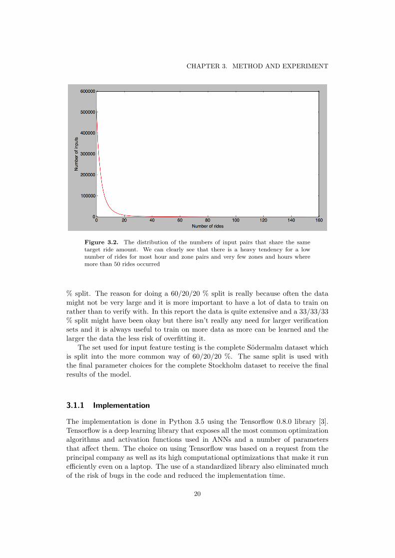
When the model is chosen, appropriate metrics will have to be used in order toget a good understanding of the performance of the network. For estimation tasksa mean of errors is often a common approach. However the mean average di�erencemethod can be bad at indicating the real performance, especially if the distributionof target outputs is not even. In figure 3.2 on page 20 we see that the distributionof output targets in the data in this paper is not even at all. Few rides are far morecommon than many rides in the di�erent hour and zone combinations. A meanerror method here might be very low if the network always output zero, since thatwill give a zero error for most cases. That low error will, however, be useless sincethe network has no capability of producing good estimations.
Overfitting problem
Overfitting, sometimes called variance, is a common problem in machine learningwhere the method learns the training data too well and fails to generalize the realdata. Overfitting can be caused either by too high adaptivity in the method, forexample too many training epochs or more hidden neurons/layers than is necessaryto describe the problem [15] or by a too small set of training data that fails torepresent the whole scope of the problem [19]. The data used in this paper isextensive and will likely be su�cient to give stable results for Stockholm. Despiteoverfitting being a problem it is often utilized when training a neural network byfirst creating a model that overfits the data, which indicates that the model isable to properly learn the problem instance, and then applying measures to avoidoverfitting [15]. A common method to reduce overfitting is to remember the currentbest weights of the model and stop training once the performance on the validationset gets worse, called early stopping [19].
Dropout
Dropout is a technique where nodes are dropped randomly during training, meaningthat they won’t a�ect the outcome for that specific training epoch. Srivastava et al.(2014) [19] claim that dropout breaks up co-adaptation between the nodes that iscreated by the training data and thus gives a more robust adaptation to real worlddata. They found that dropping 20% of the input nodes and 50% of the hiddennodes every epoch were a good approach for most networks. They also claim thatdropout increased the performance of networks in a wide variety of domains and isthus a general technique that would work for any neural network [19].
The main drawback of dropout is named as the increased computational com-plexity where the training time is increased by roughly 2-3 times in order for thetraining to converge. The authors [18] claim to have proved the strength of dropoutfor large complex networks but do not mention performance on smaller networks[19].
15

CHAPTER 2. BACKGROUND
2.4.6 Cross-validationCross validation are a series of techniques to avoid overfitting and to test the ro-bustness of a method. The concept of cross-validation is about testing and trainingon di�erent subsets of the data available [12]. The most naive way of training aneural network would be just to split the data in two sets and train on the wholetraining set until the loss stops to improve and then check the performance on thetest set, this method however is very prone to overfitting, since there is no way ofknowing when the optimization process goes from learning the relations in the datato learning exactly the points in the training set.
One of the most simple and common variants of cross-validation is to split thedata into three sets, training-set, validation-set, and test-set. The network is trainedon the training set for as long as the loss of the validation set keep improving. Thento make the performance test unbiased the network is tested on the test-set whichis essential to have since the network model will be based on both the training andvalidation sets as they have been used to determine the network model.
A problem with the three set split is that it might give good results purely bychance. If the data is not large enough or if the test set is ’easy’ for the networkto predict then one will be led to believe that the model is better than it reallyis. A common cross-validation technique to avoid this is k-fold cross-validation.The principle is to divide the data set into k subsets, and for k iterations, trainthe network using every set except k, and the validate the results with subset k.Then take the average of the results from all the k iterations as the real networkperformance [12]. This method with a proper size of k will eliminate the problemwith ’easy’ sets and give a more fair estimate of how well the network will actuallyperform on unseen data.
Kohavi et al. (1995) [9] evaluates di�erent cross-validation methods and theyclaim that 10-fold cross-validation is the optimal number to use in model selection.
2.5 Related workMukai and Yoden (2012) [14] attempted a similar way of forecasting of taxi pas-senger demand based on geographical areas and time slices. They grouped theirdata of the 25 major areas of Tokyo into time slices of four hours and predictedthe demand for every city area for the coming time slice based on the demand inthe previous four hours. This approach is a bit di�erent from the one in this paperas no fresh data will be available to predict the next set of demand outputs. Theapproach in this paper will instead be to use fewer input parameters to predict alarge output vector which will present an additional challenge.
Mukai and Yoden (2012) manages to predict the taxi demand for the regionsof Tokyo with an error ranging from 6-24% for di�erent times and zones. Theyattempt to incorporate precipitation in their results as a boolean input parameter,raining or not raining, but concludes that it has no statistical significance. How-ever, they claim that more advanced weather parameters could possibly produce
16

2.5. RELATED WORK
better predictions, such as having the rain amount as a continuous parameter oronly including it if the rain reaches a certain threshold.
Moreira-Matias et al. (2012) [13] attempt an alternative prediction method to ma-chine learning for estimating passenger demand for the coming 30 minute period,namely time series forecasting techniques on real-time GPS events transmitted be-tween 441 cars in a taxi network. They compared their real time estimation withthe actual passenger demand in 63 taxi stands in the city of Porto. Each triedmodel achieved an accuracy over 74%.
Grinberg et al. (2014) [4] did similar taxi demand forecasting to the one in thispaper using a grid split over New York city and attempting to predict the numberof rides for the grid squares for a given hour. They attempted three di�erent machinelearning approaches, linear least-squares regression, Support Vector regression andDecision Tree regression. They explore various feature sets containing zone, hour-of-day, day-of-week, and hourly precipitation. Just like Mukai and Yoden they donot find rainfall to be a statistically significant parameter.
Schaller (2005) [17] investigates a method to predict taxi car demand on a higherlevel to suggest taxi car regulation in US cities. He uses a variety of di�erent param-eters for predicting the taxi demand for US cities. Mainly population size, publictransit ridership, tourism levels, business visitors, large event activities, employ-ment levels, percentage of low income population, and vehicle ownership. Schaller(2005) uses these measures in order to predict the taxi demand for di�erent citiesbut these higher level parameters might also be used to indicate a weight change inlocal di�erences. In order to get good predictions from previous data, changes inthese parameters might be required in order to correctly find rise and decline in thedemand between di�erent years. Schaller (2005) finds that three of the parametersare extra strong in their ability to predict taxi rides, amount of car ownership, air-port activity and subway commuting, it could be interesting to incorporate theseparameters into the neural network.
17

Chapter 3
Method and experiment
The method chapter is divided into two main subparts. First the evaluation ofparameters and implementation details for the network is described. Then theevaluation of input features of the taxi estimation problem is described to see whichinput features yield the most correct results.
3.1 DataThe data available to use consists of 44 million taxi rides in Sweden with a largenumber of parameters attached to them. In this report only the area of the Stock-holm is analyzed, due to the belief that the data for the rest of Sweden would beto sparse to give stable results. Two datasets are created, one smaller for testingimplementations and one for testing the di�erent input sets the final model used.The first consists of rides in the district of Södermalm where rides for the timeperiod 2010-01-01 to 2016-02-29 are distributed over 10 di�erent zones. The ridesfor Södermalm in that period number to 4934694. The other set contain the datafor the whole city area of Stockholm where 15463312 rides in the same time periodmentioned above are distributed over 42 zones. A distribution of the number ofrides per day in this time frame can be seen in figure 3.1.
The taxi rides of the data contain only 2 parameters, an integer representing inwhich zone it occurred in the principal company’s layout maps and the time stampfor when it happened. This data is converted into data for the network by groupingall rides that occurred in the same hour, day and zone.
The zones are predefined zones over Sweden ranging in various sizes and shapesthat are used by the principal company. The converted data is constructed usingonly rides from 2010 and onwards since the amount of available data was lower forthe earlier years, omitting them should yield a more stable result. Only days whereride data exists will be taken into account and data is generated for every hourper day and for every zone. Then the rides that occurred in the retrieved data arespread out on the hours and zones. The distribution of the number of datapointswhen a certain number of rides occurred can be seen in figure 3.2.
18

3.1. DATA
Figure 3.1. The distribution of rides for all days of the selected period 2010-01-01to 2016-02-29
By spreading out the rides on the hours and zones in which they occurred,the rides of the Södermalm dataset are converted to 540240 input/output pairsand the larger dataset of Stockholm is converted into 2269008 input/output pairs.Every point in the converted datasets contain one integer representing the zone andone time stamp, with resolution in whole hours, representing the date and hourwhen the ride occurred. These two variables are mapped to a number of rides thathave occurred in that time and zone. From the time stamp we can extract severalparameters to use as input for the network. The hour is the basic one, but the datealso gives us day of the week, day of the month, month of the year etc.
Apart from the taxi ride statistics, historical weather data, provided by theSwedish Meteorological and Hydrological Institute, SMHI [20] is combined withthe datasets. The weather data consists of hourly temperature and precipitationreadings from a station in Stockholm.
The data sets used for implementation testing is done using the common training/ validation / testing split where only a subset of 24 % the data available forSödermalm is used. The sets are divided into equal thirds of 8 % of the totaldata each, this is done due to the heavy computational complexity in the trainingprocess. With 8 % of the complete data used for training decent training timescould be achieved. Because of the limited experimentation time, running each testfor several hours was not feasible. Using 8% of the data made the tests run in aboutone hour while still not compromising too much with the stability of the results.The percentage was chosen by empirical tries where it was lowered until the costvalues started to vary between the runs.
For the feature set testing the whole set of Södermalm data is used. The splittingof training, validation and test sets were chosen to be the very common 60/20/20
19
CHAPTER 3. METHOD AND EXPERIMENT
Figure 3.2. The distribution of the numbers of input pairs that share the sametarget ride amount. We can clearly see that there is a heavy tendency for a lownumber of rides for most hour and zone pairs and very few zones and hours wheremore than 50 rides occurred
% split. The reason for doing a 60/20/20 % split is really because often the datamight not be very large and it is more important to have a lot of data to train onrather than to verify with. In this report the data is quite extensive and a 33/33/33% split might have been okay but there isn’t really any need for larger verificationsets and it is always useful to train on more data as more can be learned and thelarger the data the less risk of overfitting it.
The set used for input feature testing is the complete Södermalm dataset whichis split into the more common way of 60/20/20 %. The same split is used withthe final parameter choices for the complete Stockholm dataset to receive the finalresults of the model.
3.1.1 Implementation
The implementation is done in Python 3.5 using the Tensorflow 0.8.0 library [3].Tensorflow is a deep learning library that exposes all the most common optimizationalgorithms and activation functions used in ANNs and a number of parametersthat a�ect them. The choice on using Tensorflow was based on a request from theprincipal company as well as its high computational optimizations that make it rune�ciently even on a laptop. The use of a standardized library also eliminated muchof the risk of bugs in the code and reduced the implementation time.
20

3.2. OPTIMIZING THE NETWORK
3.2 Optimizing the networkIn order to find the optimal neural network to use for the taxi demand estimationproblem di�erent parameters for the network implementation are trained and testedwith the subset of the Södermalm data mentioned earlier. This dataset shouldbe su�cient to decide which network parameters work best for estimating taxidemand. During this implementation parameter testing the data is divided intothree chronologically ordered datasets, the training set, the validation set and thetest set. The network architecture and implementation choices are tuned for themost basic parameters which are believed to be the most important ones, namely,zone, hour-of-day and day-of-week.
3.2.1 Metrics for network optimizationTo measure the performance of di�erent network architectures two di�erent valueswill be observed. Most importantly is the loss function convergence, which indicatesif the network is actually getting better at estimating the data. Fast convergencerate in combination with the ability to reach a low final loss value is the mostessential properties when training a neural network.
In order to get a performance variable that is a little bit easier to comprehend,the ’accuracy’ measure will be included as well. The accuracy of the network whichis defined as mean error, the average distance from the predictions, y
p
, and thecorrect output in the test-set y.
accuracy = mean(|y ≠ y
p
|)
Thusly, an accuracy score of 2.5 would mean that on average, the network guessesare 2.5 rides o� from the target.
3.2.2 Loss functionThe loss function for the optimization is chosen as mean squared error, loss =mean((y ≠ y
p
)2). It is important for the loss function not only to minimize theaverage di�erence between y and y
p
but also take into account that the data containmany points with few number of rides and few points with a large number of rides.
Two other loss functions were attempted, mean error, and mean error to thepower of three. The mean error loss = mean(|y ≠ y
p
|) doesn’t penalize outputtargets of large ride quantities in a reasonable way so it will likely give unfairaccuracy values. Using the mean error function with the data available would likelycause the network to output zero very often as that is the most common output,and no penalization would be taken against guessing very badly. Meaning that itwill be able to lower the loss and consequently the accuracy measure accuracy =mean(|y ≠ y
p
|) by being very correct for the quantitative amount of data pointswith a low ride target, and at the same time being very bad at the fewer pointswith a high ride target.
21

CHAPTER 3. METHOD AND EXPERIMENT
In order to combat the loss function not taking large output values into ac-count the function loss = mean(|(y ≠ y
p
)3|) was attempted which heavily penalizesdi�erences for the data points with large ride numbers but no clear improvementwas found to the chosen loss function, thus mean squared error was chosen as lossfunction.
3.2.3 Architecture
The architecture of the network has to be tailored for the problem that we are tryingto learn. For example a network of only a single node in the layer before the outputwill not be able to generalize at all but will, if trained properly, only output theaverage answer through every training example. In the same sense a too complexnetwork with too many layers and neurons will be very computationally expensiveand might be more prone to overfitting and learning special cases rather than thegeneral problem. The challenge here is to find the minimal network architecturethat properly learns the problem.
Input and Output layers
The input layer will have as many nodes as we choose our input to be, if 5 inputsare used then the input layer will have 5 nodes. The size of the output layer willdepend on what problem you are trying to solve. If you are doing classificationwith 10 di�erent classes then the output layer would consist of 10 nodes. In theseexperiments the only target is to output a value. Therefore the output layer willhave only one node.
Hidden neurons
To find a good number of hidden neurons to use in the hidden layers, a networkwith di�erent amount of hidden neurons is tested with the ADAMOptimizer algo-rithm and the hyperbolic tangent activation function as they are claimed to be thebest general optimizer and activation functions according to Kingma et al. (2014)and LeCun (2012) [8] [11]. Initially, a network with only a single hidden layer isattempted with 20, 80, 150 and 450 neurons for which the results can be seen insection 4.1.1.
Hidden layers
To find a good choice of hidden layers a network is tested with the ADAM optimizeralgorithm and the hyperbolic tangent activation function for each hidden layer. Fourdi�erent layer sizes, 1,2,3,4 respectively, are attempted with a size of 150 hiddenneurons per layer and the results as seen in table 4.3 in section 4.1.2.
22

3.3. INPUT PARAMETER EXPERIMENTATION
Optimization algorithm
For an optimization algorithm to be good it should converge relatively quickly andpreferable not get stuck in a bad local optima. Three optimization functions aretested with the symmetric sigmoid hyperbolic tangent as activation function in eachlayer as it is claimed to be the strongest general activation function.
The three attempted algorithms are Stochastic Gradient Descent, RMSProp,and Adam. The optimization testing is done using a network of three layers with150 neurons in each and with 500 training epochs. The results are presented in theresult section: 4.1.3.
Activation functions
Four di�erent activation functions are evaluated. The ones chosen to be testedare the two most common sigmoid functions as well as ReLU and ReLU6, whichare claimed to perform better in deep networks and networks with output targetsover 0. In order to reduce the number of options the same activation function willbe chosen for each layer except for the output layer which will have the identityfunction in order to get regression behavior. The results can be seen in the section4.1.4.
Overfitting
In an attempt to combat overfitting a training sequence that forces overfitting is cre-ated where a three-layered network with 150 neurons in each hidden layer is trainedfor 2000 epochs using the hyperbolic tangent activation function and ADAMOpti-mizer with all the available input parameters. Dropout is then applied in two vari-ations. First with the levels suggested by Srivastava et al. (2014) of 20% dropoutin the input layer and 50% dropout in the hidden layers [19]. Then also with amilder level of dropout where only 10% of the input nodes are dropped and 20% ofthe hidden nodes. The comparison of the di�erent techniques can be observed insection 4.1.5.
3.3 Input parameter experimentationThe two basic parameters that formulate the base of each input case are:
• zone, the zone where the ride originated, where the zones are represented byintegers from 0 to the number of zones minus one
• hour, the hour of the ride, represented by integers in the range [0, 23]
A survey was conducted at the principal company about what additional informa-tion could influence the taxi demand. A variance over the days of the week seemsto be the most obvious one. A variance over the month should also be apparentas taxi ridership is somewhat considered a form of luxury travel in Sweden and
23

CHAPTER 3. METHOD AND EXPERIMENT
household spending increases after the Swedish payday, the 25th of every month.Additionally there is a significant increase in activity of the nightlife scene after theSwedish payday which is commonly tied to taxi ridership in Stockholm. To betterreflect this the parameter day of the month will be modified to be ’days after the25th’, which would indicate a larger household spending and possible increase inridership for low values of this parameter.
The principal company also acknowledged that good weather during the summermonths (which can also be observed in figure 3.1) caused the taxi demand to dropsignificantly which leads one to believe that the month of the year would be relevant.As mentioned weather is a possible factor as well, heavy precipitation could lead tomore spontaneous taxi rides, but a more steady prediction might be gained fromobserving temperature which is not as locally occurring as rain or snowfall, sincemost data points contains zero rainfall it is reasonable to assume that combiningprecipitation with temperature would give a more clear estimate of good or badweather.
The extra input features chosen were the ones in the survey among the principalcompany for which reliable data could be gathered for all points. The final inputfeatures chosen for testing are as follows, all features are floats normalized to therange [0,1].
• day-of-week, the day of the week when the ride occurred, represented by inte-gers on the range [0, 6]
• day-of-month, the day of the month when the ride occurred, modified so thatthe first day is the 25th which is the most common Swedish payday, repre-sented by integers on the range 0 to the number of days in the month
• month, the month of the year when the ride occurred, represented by integerson the range [0, 11]
• temperature, the temperature of Stockholm when the ride occurred, repre-sented by a float in the range [0, max(temp) + abs(min(temp))]
• precipitation, the accumulated rainfall of Stockholm in the hour that the rideoccurred, represented by a float of the rain amount in millimeters
The feeding of the parameters as continuous discrete values can be argued toa�ect the outcome in some ways. Since the neural network base its decisions andtraining on additive and multiplicative operations it will treat the hour 4 moresimilarly to the hour 5 than 9. This might seem logical since the taxi ridershiplevels likely follow some curve over the course of the day. However, this will nothold for the hours 0 and 23, which the network will have to learn to treat similarlysince they are equally close to each other as hours 4 and 5 and likely have similar taxiridership levels to each other. Hopefully, the network will learn to make distinctionsbetween these values.
24

3.3. INPUT PARAMETER EXPERIMENTATION
In the same way it might seem odd to input the zone as a continuous discreteID since the zones geographical properties might not be similar at all. Another ideamight be to feed the zones as many di�erent input variables with the values 0 or 1depending on which zone it is. However, this realization occurred a bit late in theproject progress and will be considered as future work. All the variables will be fedas continues values for the experiment of this project.
The features are grouped into five sets, which are tested and examined. Set 1 isthe minimal set, only containing the two parameters that are required for testing,this set is thus the same data used for the baseline predictions. Set two is theminimal set with the day of the week included, this parameter is believed to be thestrongest one except hour and zone for predicting taxi demand. A variance patternover the week seems to be the most probable of all the tested parameters.
Set 3 includes the monthly parameters to the second set which will indicateif day-of-month and month-of-year are relevant in predicting taxi demand whencompared to the results of Set 2. Set 4 is the basic set with weather data includedwhich will indicate if weather is a relevant factor when predicting taxi demandwhen compared to Set 1. Finally Set 5 contains all the parameters which wouldlikely be the best set if all the parameters attempted are in fact relevant. A clearerdescription of the feature sets is presented in table 3.1
Table 3.1. The feature sets for testing
Feature set number Features1 - basic zone
hour2 - basic + week zone
hourday-of-week
3 - basic + week/month zonehourday-of-weekday-of-monthmonth-of-year
4 - basic + precipitation zonehourprecipitationtemperature
5 - all zonehourday-of-weekday-of-monthmonth-of-yearprecipitationtemperature
25

CHAPTER 3. METHOD AND EXPERIMENT
3.3.1 Validation technique10-fold cross validation is applied to the input testing in order to receive robust re-sults as Kohavi claims it to be a strong cross-validation approach for model selection[9].
K-fold cross-validation seems to be a solid choice to use for testing the networkparameters. However, in this report the problem has a chronological aspect as wellthat makes the three subset split interesting to use. Since the point of the networkis to be able to predict future rides, splitting the dataset into three chronologicalparts will be interesting in order to see how predicting future values actually fares.The dataset should be su�ciently large that it becomes unlikely that the test-setwill become an ’easy’ set to predict by chance.
3.3.2 BaselineThe performance of the network using the di�erent feature sets will be measuredin a number of ways and compared with each other. However, in order to get anunderstanding of how well the network models are actually performing they will becompared against a baseline value as well. The baseline will be an average using thewhole dataset over the two basic variables, zone and hour of the day. The baselinewill thus be a very basic way of guessing taxi demand based on simple averages.The least you could expect from a correctly implemented and trained network modelwith additional parameters that a�ect the demand is to beat this baseline.
3.3.3 Metrics for feature testing and final network validationDuring the testing of the implementation parameters the metrics Accuracy andLoss were observed and used. However, in order to both get a better idea of howgood the networks predictions actually are and to be able to better distinguish theperformance between the attempted feature sets, two additional metrics will beobserved.
In order to give a more comprehensible understanding of how well the network isperforming the ’correct’ metric will be introduced. A guess will be called correct ifit is su�ciently close to the real answer. This metric will be defined as the numberof predictions that lie within a threshold of 30%, or 1 ride from the correct answer.The boundary of 30 % and 1 was chosen arbitrarily together with the principalcompany as a measurement that would give an understanding of how often themodel make a reasonably correct answer. Hopefully it should give the reader anumber that they feel represents how well the network is guessing.
correct =I
y
p
> 0.7 ú y · y
p
< 1.3 ú y if y > 0, or
y
p
> y ≠ 1 · y
p
< y + 1 if y Ø 0
The other metric is added to get some additional certainty in the comparisonbetween di�erent feature sets. Since the amount of customers that order taxi within
26

3.3. INPUT PARAMETER EXPERIMENTATION
an hour and zone is a stochastic variable. The definition of Poisson distribution givesus the probability of an event occurring k times in an interval where ⁄ is the averageoccurrence rate.
P (x) = e
≠⁄
⁄
x
x!If the network is making proper estimations then it should have learned the
average rate of car occurrences given the input parameters for an hour and a zone.This means that if we, for each data point in the set used for verification, use theprediction as ⁄ in the Poisson formula and run it with k as the real answer, wewill get the probability of the network being correct in that estimation. To get avalue that represents the likelyhood that all guesses are correct the product of thesepoisson values will be used. Since this final value will likely be very small and oftenrounded to 0 the product will be represented by the sum of the natural logarithmsof the poisson values, in order to get it on a better scale.
Including these two metrics should give the readers an idea of how well thenetwork is guessing as well as make sure that the comparisons between the di�erentfeature sets are actually valid.
3.3.4 Final testingAll the feature sets will be tested with a network with the parameters defined insection 4.1.6 on the full dataset for Södermalm using both chronological validationwith the training/validation/test split defined in section 3.1. The complete datasetfor Stockholm will the be tested using the feature set with the best results for finalresults for the taxi estimation of Stockholm. The final result will be verified usingboth chronological and 10-fold validation for robustness.
27

Chapter 4
Results
This chapter will present the results of the two main tasks of this report, finding theoptimal network architecture for estimating taxi demand and finding the optimalinput features for estimating taxi demand.
4.1 Architecture evaluationIn this section the results of the network architecture experiments will be presented.Even though the baseline is not trained in any way the loss and accuracy values canbe calculated for the baseline predictions using the same data as the testing to geta reference of how the di�erent setups compare.
Table 4.1. Loss and Accuracy values for the baseline using the subset of the Söder-malm data
Loss Accuracy102.41 4.77
4.1.1 Hidden neuronsThis section contains the results of the experiment with di�erent number of hiddenneurons for the network architecture.
Table 4.2. Comparison between di�erent hidden neuron numbers for a single layerednetwork using the hyperbolic tangent activation function. The network is trainedusing ADAMOptimizer until no improvement on loss is made for five epochs
Neurons Loss Accuracy20 146.17 6.1380 115.78 5.76150 104.04 5.44450 97.61 5.18
28

4.1. ARCHITECTURE EVALUATION
The baseline achieves a Loss and Accuracy measure of 102.41 and 4.77 respec-tively, as seen in table 4.1. If we compare this to the neauron amount trials in4.2 we see it has a loss value in the same area as the networks with the two largerneuron sizes, but a better accuracy value. It is likely that the baseline is more proneto outputing very low values, since most datapoints have a target that is very low.This in turn would mean that since most of the data points are zero or very low,the baseline method will get a good average di�erence between the guesses and realvalues. Notable here is that none of the di�erent attempts with a single layerednetwork is able to beat the baseline in accuracy indicating that a single layerednetwork is not able to generalize the problem properly.
The loss function achieves a lower minimum with the increase in hidden neuronsbut the improvement between 150 and 450 seems to be diminishing indicating thatit might be wiser to increase the number of layers instead. A layer size of 150hidden neurons should be a good enough to solve the problem. The 450 neuronsincreased the computational complexity to an unrealistic level even for a singlelayered network 150 will be chosen as the hidden neuron number for each layeraccording to the rule proposed by Ng (2012) [15], that all hidden layers have thesame number of neurons.
4.1.2 Hidden layersThis section contains the results of the experiment with di�erent number of hiddenlayers for the network architecture.
Table 4.3. Comparison between di�erent number of hidden layers with 150 neu-rons each. The hyperbolic tangent is used as activation function and trained usingADAMOptimizer until no improvement on loss is made for five epochs
Layers Loss Accuracy1 114.28 6.742 54.46 4.003 40.96 3.384 40.58 3.28
It is clear from table 4.3 that the neural network can learn the problem a lotbetter when we increase the number of hidden layers above one. However, the benefitseems to diminish when going from three to four layered networks. This leads tothe conclusion that a network architecture with three hidden layers is su�cient todescribe the taxi estimation problem.
If we compare the values in table 4.3 once again against the baseline valuesin table 4.1 it is clear that the networks are better than the baseline even withtwo hidden layers, and three and four hidden layers outperform the baseline evenfurther.
The network with three hidden layers is compared again with 150, 250 and 450neurons to see if any further improvement can be made by adding new neurons, the
29
CHAPTER 4. RESULTS
results can be seen in table 4.4.
Table 4.4. Comparison between di�erent number of neurons in a net with threehidden layers, hyperbolic tangent activation functions and ADAMOptimizer
Neurons Loss Accuracy150 43.43 3.39250 43.96 3.54450 43.95 3.37
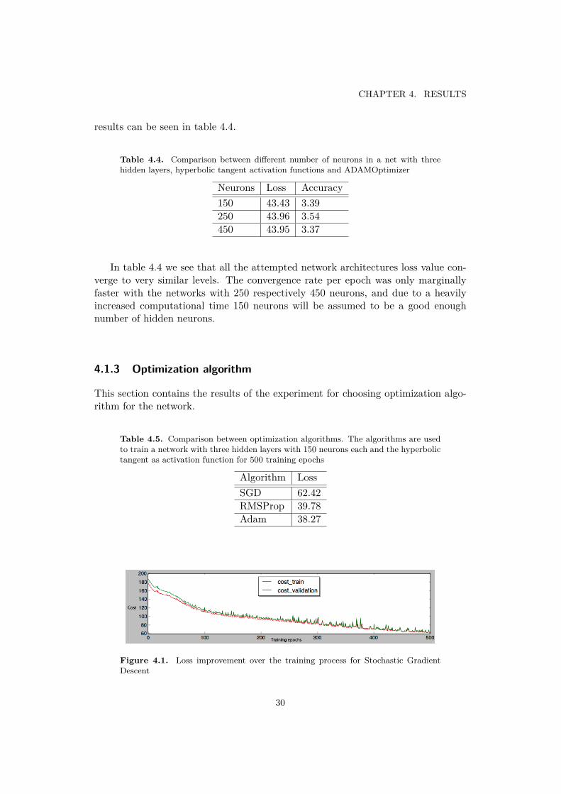
In table 4.4 we see that all the attempted network architectures loss value con-verge to very similar levels. The convergence rate per epoch was only marginallyfaster with the networks with 250 respectively 450 neurons, and due to a heavilyincreased computational time 150 neurons will be assumed to be a good enoughnumber of hidden neurons.
4.1.3 Optimization algorithm
This section contains the results of the experiment for choosing optimization algo-rithm for the network.
Table 4.5. Comparison between optimization algorithms. The algorithms are usedto train a network with three hidden layers with 150 neurons each and the hyperbolictangent as activation function for 500 training epochs
Algorithm LossSGD 62.42RMSProp 39.78Adam 38.27
Figure 4.1. Loss improvement over the training process for Stochastic GradientDescent
30

4.1. ARCHITECTURE EVALUATION
Figure 4.2. Loss improvement over the training process for RMSProp
Figure 4.3. Loss improvement over the training process for Adam
It seems from table 4.5 that the RMSProp and Adam optimizers outperformStochastic gradient descent and are able to converge to better values. RMSPropand Adam seems to converge to roughly the same value but Adam has a muchsmoother and faster convergence rate, as seen in figures 4.1, 4.2, and 4.3, and seemsto be the best choice for optimization algorithm.
4.1.4 Activation function
This section contains the results of the experiment with di�erent activation functionsfor the network architecture.
Table 4.6. Comparison between activation functions. A network of three layerswith 150 neurons each is trained using ADAMOptimizer until no loss improvementhas been done for five training epochs
Function Loss AccuracyReLU 62.73 4.78ReLU6 49.00 3.86Sigmoid 62.09 4.10Tanh 43.56 3.42
As seen in table 4.6 the ReLU6 and Tanh converges to clearly better values thanthe ReLU and Logistic Sigmoid functions do.
31

CHAPTER 4. RESULTS
Figure 4.4. Loss improvement over the training process with Rectified Linear Unitactivation functions
Figure 4.5. Loss improvement over the training process with ReLU6 activationfunctions
Figure 4.6. Loss improvement over the training process with Logistic Sigmoidactivation functions
Figure 4.7. Loss improvement over the training process with Hyperbolic Tangentactivation functions
We see in figures 4.4, 4.5, 4.6, 4.7 that the logistic sigmoid is seems to be lackingagainst all other functions in terms on convergence rate. It also seems that ReLU6and Hyperbolic Tangent converges to significantly lower values. Since the HyperbolicTangent performed best in all measures in table 4.6 including convergence rate itwill be chosen as the activation function for all the hidden layers of the network.
32

4.1. ARCHITECTURE EVALUATION
4.1.5 Overfitting
This section contains the results of the experiment to combat overfitting whentraining the network.
Table 4.7. Comparison between training attempts with di�erent levels of dropout onall features after 2000 epochs. The training was done on a network with three hiddenlayers with 150 neurons in each using the hyperbolic tanget activation function andADAMOptimizer
Dropout input layer Dropout hidden layers Loss training-set Loss validation-setNone None 13.49 53.4710 % 20 % 85.49 95.2620 % 50 % 134.76 141.26
Figure 4.8. Training process over 2000 epochs using all input features and with nocountermeasures taken to overfitting. It is clear that overfitting starts to occur aftera couple of hundred training epochs and the curves diverge from each other.
33

CHAPTER 4. RESULTS
Figure 4.9. Training process over 2000 epochs with all features with a dropout of20 % on the input layer and 50% on the hidden layers
Figure 4.10. Training process over 2000 epochs with all features with a dropout of10 % on the input layer and 20% on the hidden layers
We see in figure 4.8 that the loss for the training and validation sets starts todiverge after 200 training epochs, indicating that the neural network is over trainedon the training set and loses it’s generalization ability on unseen data. We can alsosee that the error estimates in these graphs starts to diverge which proves that thenetwork gets worse at predicting unseen data while getting better at estimating thetraining set which is a clear indication of overfitting.
In figure 4.9 we can see the application of the higher level of dropout. It isobvious that this prevents the network from overfitting and the two curves followeach other better. However, with these high levels of dropout the network is notable to converge to a very good loss value.
In figure 4.10 we can see the application of the lower level of dropout. Thislevel allowed the network to converge to a lower loss function value but still someoverfitting can be seen after about 1000 epochs.
34

4.2. FEATURE SET EVALUATION
Due to the fact that dropout implementations seems to become unable to con-verge to nowhere near the same level of the loss function value as the non-dropoutversion, as seen in table 4.7, dropout will not be used for the final testing and earlystopping will be the only measure taken to avoid overfitting. Early stopping willbe activated when the validation set loss has not improved over 5 training epochs,meaning if no improvement has been made over five complete training rounds itshould be safe to assume that the loss value will not converge much further.
4.1.6 Final network implementation parametersBased on the results above these parameters were chosen for the final architectureof the network to use on the input feature testing.
• Hidden neurons, 150 per layer
• Hidden layers, 3
• Loss function, Mean squared error
• Optimization algorithm, ADAM optimizer
• Activation functions, Hyperbolic tangent for hidden layers, linear for outputlayer
• Overfitting prevention, early stopping after five training epochs without im-provement in the loss of the validation set.
4.2 Feature set evaluationIn this section the results of the performance of the constructed ANN with thedi�erent feature sets will be presented. The results for the baseline measure willalso be included to indicate the performance of the network against a very trivialmethod.
Table 4.8. Comparison of loss results between the feature sets for one full trainingrun per set
Feature set Training loss Validation loss Test loss1 116.84 111.14 114.742 40.04 39.87 41.063 38.24 38.77 39.164 117.39 112.23 115.895 38.66 39.44 40.08
In table 4.8 the result of the training processes can be seen for the di�erentfeature sets. Sets 2, 3 and 5 all seem to reach similar loss values that are significantly
35

CHAPTER 4. RESULTS
lower than the ones reached by set 1 and 4. Clearly indicating that these three setsshare a variable that is very significant to the results, most likely day-of-week sincesets 2 and 3 seems to be performing similarly.
Table 4.9. Comparison of accuracy between the feature sets with chronologicalvalidation
Feature set Accuracy test-set Corrects test-set Loss test-set Poisson test-setBaseline 5.08 0.39 112.57 -443 9981 5.14 0.38 114.74 -454 4312 3.36 0.47 41.06 -302 3953 3.30 0.47 39.16 -302 7454 5.30 0.37 115.89 -455 3515 3.26 0.49 40.08 -297 079
In table 4.9 the results using chronological validation of the di�erent feature sets.The results of the di�erent metrics mirror the results of the training process in table4.8. Notable is that the baseline has a higher chance of making accurate predictionsthan the neural network using feature sets 1 and 4 according to the poisson andaccuracy metrics. It is also clear that sets 2, 3 and 5 perform very similarly whichleads to believe that the di�erence in their parameters does not seem to matter thatmuch. Rather that the parameter they share is a very relevant one.
Table 4.10. Comparison of accuracy between the feature sets with 10-fold validation
Feature set Accuracy Correct predictions Loss PoissonBaseline 5.08 0.39 113.37 -740 8601 5.22 0.37 115.35 -757 2292 3.36 0.48 41.09 -505 0083 3.28 0.49 38.69 -498 0284 5.21 0.37 115.56 -761 4405 3.25 0.50 38.81 -495 929
In table 4.10 we see the results when using the k-fold validation. Note thatthe scale of the poisson value di�er between the sets in tables 4.9 and 4.10, that isbecause the value of it is dependant on how many data points that are measured.If we look at the other metrics the results are similar to the ones received in thechronological validation seen in table 4.9. This indicates that the data set used islikely su�ciently large and homogeneous enough that extreme cases in the data donot a�ect the result of the predictions very much.
4.2.1 Prediction result plots from chronological validationIn order to show how the networks using the di�erent feature sets performed, plotsof the results on the test set for each network will be shown below as well as the
36

4.2. FEATURE SET EVALUATION
values for the baseline.
Figure 4.11. Predictions for the baseline approach of the average ride value foreach hour per day and zone. X-axis is the target number of predictions, Y-axis is thepredicted number and the red line indicate perfect predictions
Figure 4.12. Predictions for model trained using feature set 1. X-axis is the targetnumber of predictions, Y-axis is the predicted number and the red line indicate perfectpredictions
37

CHAPTER 4. RESULTS
Figure 4.13. Predictions for model trained using feature set 2. X-axis is the targetnumber of predictions, Y-axis is the predicted number and the red line indicate perfectpredictions
Figure 4.14. Predictions for model trained using feature set 3. X-axis is the targetnumber of predictions, Y-axis is the predicted number and the red line indicate perfectpredictions
38
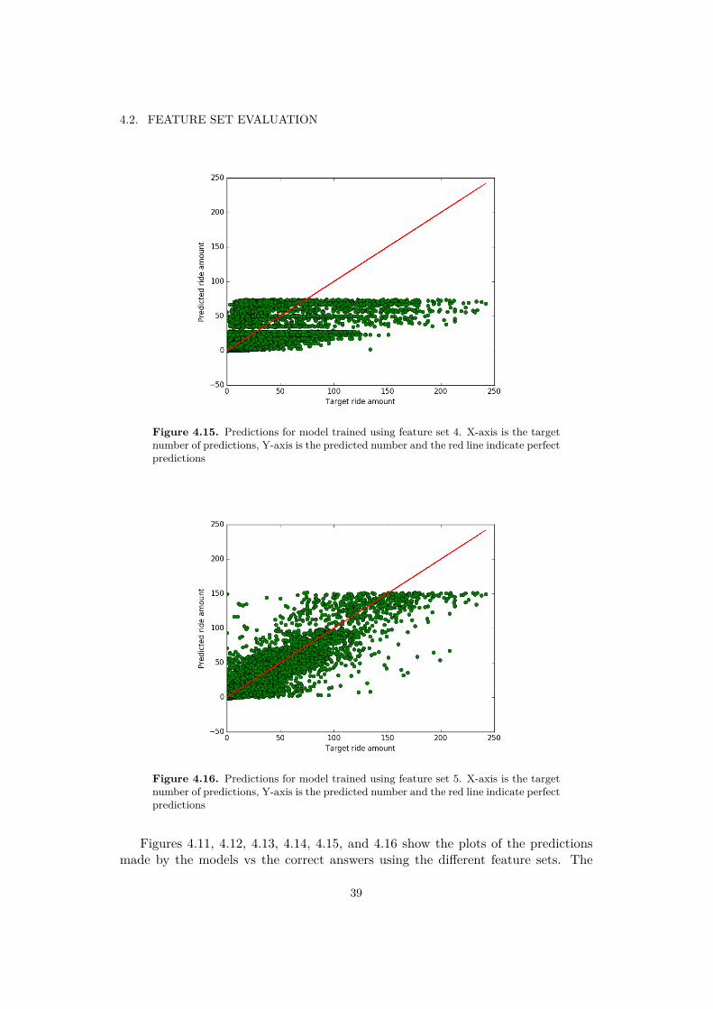
4.2. FEATURE SET EVALUATION
Figure 4.15. Predictions for model trained using feature set 4. X-axis is the targetnumber of predictions, Y-axis is the predicted number and the red line indicate perfectpredictions
Figure 4.16. Predictions for model trained using feature set 5. X-axis is the targetnumber of predictions, Y-axis is the predicted number and the red line indicate perfectpredictions
Figures 4.11, 4.12, 4.13, 4.14, 4.15, and 4.16 show the plots of the predictionsmade by the models vs the correct answers using the di�erent feature sets. The
39

CHAPTER 4. RESULTS
x-axis represent the target values and the y-axis represent the predictions madeby the models. The red line represents the distribution of what would be perfectpredictions. We can see how adding certain parameters clearly increase the networksabilities to predict higher quantities of rides. Set number one for example looksvery similar to the baseline when plotted, because they are based on the same data.Using only these few parameters the network does not have enough information tobase the decisions on and will just output an average of the trained data, exactlylike the baseline is doing. Interesting to note can be that while sets two and threeseems to perform similarly according to tables 4.9 and 4.10. Their plots are notvery really similar. Since the network using feature set 2 has less variables to basethe predictions on we get a lot of predictions on the same value, since there is noinformation that the network can use to distinguish the predictions further.
Important to know here is that the scores on the entire test-set of the Södermalmdataset is plotted in these plots, which means the amount of points in the graphsare roughly 108 000. When looking at for example plot 4.14 we can distinguishthese points quite clearly in the top right corner, indicating that they are quite fewand probably hard points to predict. In contrast looking at figure 3.2 indicates thatthe vast majority of the points are actually located far down on top of each otherin the left corner.
4.3 Performance of final network model
In this section the performance of the training and predictions of the final networkwill be presented. The network is trained on the complete dataset of Stockholmwith the parameters described in section 4.1.6 and feature set #5. Set 5 is chosenbecause it was the best performing feature set according to tables 4.9 and 4.10,despite the fact that weather did not seem to a�ect the results very much whencomparing set 1 and 4.
Table 4.11. Scores for the final network model with the two validation methodscompared to the baseline. The poisson metric is excluded for the cross validatednetwork as that model uses a smaller data set for validation and the poisson metricis dependent on the same validation set in order to be fair.
Accuracy Corrects Loss PoissonBaseline 3.74 0.43 65.12 -1 508 804Chronological validation 2.72 0.46 26.21 -1 132 40310-fold validation 2.73 0.45 27.04
In table 4.11 we see that the network predictions get a smaller distance to thevector of correct targets than the baseline which means that on the total averagethe network is guessing about 1 ride better than the baseline. The poisson metricalso indicates that the network is better than the baseline.
40
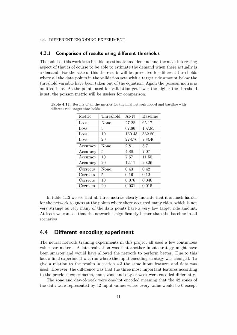
4.4. DIFFERENT ENCODING EXPERIMENT
4.3.1 Comparison of results using di�erent thresholdsThe point of this work is to be able to estimate taxi demand and the most interestingaspect of that is of course to be able to estimate the demand when there actually isa demand. For the sake of this the results will be presented for di�erent thresholdswhere all the data points in the validation sets with a target ride amount below thethreshold variable have been taken out of the equation. Again the poisson metric isomitted here. As the points used for validation get fewer the higher the thresholdis set, the poisson metric will be useless for comparison.
Table 4.12. Results of all the metrics for the final network model and baseline withdi�erent ride target thresholds
Metric Threshold ANN BaselineLoss None 27.28 65.17Loss 5 67.86 167.85Loss 10 130.43 332.80Loss 20 278.76 763.46Accuracy None 2.81 3.7Accuracy 5 4.88 7.07Accuracy 10 7.57 11.55Accuracy 20 12.11 20.26Corrects None 0.43 0.42Corrects 5 0.16 0.12Corrects 10 0.076 0.046Corrects 20 0.031 0.015
In table 4.12 we see that all three metrics clearly indicate that it is much harderfor the network to guess at the points where there occurred many rides, which is notvery strange as very many of the data points have a very low target ride amount.At least we can see that the network is significantly better than the baseline in allscenarios.
4.4 Di�erent encoding experimentThe neural network training experiments in this project all used a few continuousvalue parameters. A late realization was that another input strategy might havebeen smarter and would have allowed the network to perform better. Due to thisfact a final experiment was run where the input encoding strategy was changed. Togive a relation to the results in section 4.3 the same input features and data wasused. However, the di�erence was that the three most important features accordingto the previous experiments, hour, zone and day-of-week were encoded di�erently.
The zone and day-of-week were one-hot encoded meaning that the 42 zones ofthe data were represented by 42 input values where every value would be 0 except
41

CHAPTER 4. RESULTS
the index corresponding to the id of the zone for that input. The same encodingwas used for the day-of-week parameter with 7 di�erent input nodes.
The hour parameter was still fed as a continuous value but the break point wasshifted. Instead of shifting from 23 to 0 in a rather busy hour of the night the shiftwas moved so that 0 represents 5 in the morning and 23 represents 4 which are thetwo least busy hours of the day. The hypothesis here was that going from 23 to0 should now be less of a disturbance for the network. That disturbance will stillexist but for data points later at night, but as a larger portion of these hours havefew or no rides, the network will hopefully be better at forecasting them.
Table 4.13. Scores for the final network model using the di�erent input encodingdescribed in section 4.4
Accuracy Corrects Loss Poisson2.52 0.50 25.22 -1 083 812
According to table 4.13 it seems like using the di�erent encoding yields a clearlybetter result. The network trained with this encoding beats the network in section4.3 in every metric, although not by extreme levels. The di�erence is most likelydue to the fact that it will be easier for the network to distinguish di�erent inputvalues compared to the other technique.
42

Chapter 5
Discussion and Conclusions
In this chapter the results and thoughts about them will be presented.
5.1 Loss function convergence
Neural networks were trained using all the attempted feature sets and the loss valuefor all sets converged during the training, indicating that the variables fed at leastgive some hint of how to estimate taxi demand. The metrics in tables 4.9 and 4.10show that even the worst feature sets perform roughly at the same level as thebaseline, and there is a clear di�erence in performance compared to the best featuresets. This shows that the network is actually able to utilize the input it is given ina productive way, at least to some extent.
The validation and training loss follow each other very tightly which is a bitunusual but can probably be explained due to the fact that the data is very extensiveand is very homogeneous in its samples, many of them being very similar. This giveslittle room for hard or strange examples in the data to have a very large e�ect onthe loss value which is an average of all the samples. Typically the training requiredsome 5-100 epochs to complete. The fact that overfitting only started to occur afterabout 200 epochs were forced in section 4.1.5 supports the theory above.
5.2 Input variable encoding
In section 4.4 a short experiment to change the input strategy is shown. It seemsobvious from this experiment that the input could be fed in a better way andthus allowing the network to generate better results. However the di�erence wasonly minor and it seems like choosing the right input features is more importantthan choosing input strategy. Although it is possible that even better results couldhave been received if the network architecture was based on experiments using thisimproved input encoding.
43
CHAPTER 5. DISCUSSION AND CONCLUSIONS
5.3 Feature sets
The horizontal lines that can be seen for the baseline results in figure 4.11 canclearly be seen in the performance of feature set 1 in figure 4.12. In table ref 4.9 thevalues for the baseline and feature set 1 also performs similarly, this is not strangesince both methods have exactly the same information to base their decision on.The neural network seems to learn the average that is manually calculated for thebaseline predictions as intended.
It also seems to be clear, from table 4.8 and table 4.9, that the day of the week isthe strongest indicator of the taxi ridership levels. The two sets lacking this featureperform almost as badly as the baseline while the three sets that have this featureall perform significantly better in all metrics.
When we include day of the month and month we see some extra improvementon all metrics that indicates that taxi ridership also follow some monthly and yearlypatterns, which figure 3.1 also hints about. However the improvement is minimaland does not contribute nowhere near as much as day of the week.
Just as Mukai and Yoden (2012) [14], and Grinberg et al. (2014) [4] finds,weather does not seem to be a relevant factor for predicting taxi ridership. Nosignificant di�erence in the accuracy metrics can be found between feature sets 1and 4, only that set 4 actually seems to be performing worse. The di�erence inspread of the predictions in figure 4.14 contra figure 4.12 can probably largely becontributed to noise generated by the weather data in the network rather than anyadded strength in predictability.
Feature set 5 seems to perform a little better than set 3 but this di�erence canprobably be discarded as noise and randomness. From figure 3.1 we clearly seea tendency of lower taxi ridership during the summer. According to the surveyamong taxi drivers conducted at the principal company ’good’ weather was a clearindication of a lower level of taxi ridership. Arguably, this correlation is captured bythe month and day-of-month features rather than the two weather features whichwould indicate that a general good weather, which is usually the case during thesummer, is a more important factor than temporary factors such as rain. However,it might be possible that the weather features can help the predictions only whenthey are combined with either of the features day of month or month of year. Thatmight explain why set 5 seems to be marginally stronger since set 3, however, thatcan not be said for sure as the di�erences are so small.
The quality of the rain data can be debated. If you think practically then rainwould only have a real e�ect on spontaneous taxi rides as most people would planahead for a rainy day and take the public transit and/or bring an umbrella. Therain and temperature features used here are only unique for each day and hour forStockholm, not per zone. Hence, for the rain to be an e�ective parameter the datashould preferably be available as individual measurements for each zone, then highlevels of precipitation for a small defined area could possibly be a clearer factor forspontaneous taxi rides than just a rainy or cold day in general.
44

5.4. NETWORK PERFORMANCE
5.4 Network performance
Arguable the optimal network implementation is not yet found. The network wastuned only for the basic feature set and day of the week with the assumption that itwould perform appropriately for the other feature sets as well. It is possible that thelarger feature sets would require more hidden neurons or even more hidden layers inorder for the network to properly capture the feature relations and make accuratepredictions. However, a simple trial with 250 hidden neurons for the full feature setwas conducted and it did not show any improvement over the 150 neuron networkthat was used for the results.
The overfitting problem was addressed in section 3.2.3 and in the end only thesimplest countermeasure was taken to prevent it. It is possible that the failure toget good convergence rates were caused by the neurons of the network being toofew when dropout was applied. Increasing the number of hidden neurons in thelayers in combination with dropout could possibly have made the network learn theproblem better.
5.5 Evaluation metrics
The accuracy metric is a practical one that states how close the network is fromoptimal performance, an accuracy result of 0 would mean that the network is 100% correct when making guesses. However, this metric is not descriptive enough ofthe actual performance to dare base taxi distribution upon. As mentioned earlier,a solution that only guessed zero might still get a pretty good accuracy value.
To increase the comprehensibility of the results the ’Correct predictions’ met-ric was added. The goal was that this metric would give the reader an intuitivedescription of how many guesses were ’correct’ where correct was defined as beingsu�ciently close. The desire here was to give meaning to the results to the reader,the poisson or loss metrics does not really give a human a good understanding ofwhat the model can do, they are best suited for comparison against other models.
The Poisson metric was added to give a more scientifically fair comparativeresult. The poisson values are the likelyhood that the network is actually correctgiven the actual correct answers. However, since the Poisson results indicate howprobable it is for the network to guess exactly correct, it is not a very fair metricfor human intuition.
Even though all metrics used might have their own flaws the combined use ofall give a good description of the performance of each model and make them easyto compare. The di�erent metrics are also quite unanimous in their decision of bestmodel.
45

CHAPTER 5. DISCUSSION AND CONCLUSIONS
5.6 Best results
The best results were achieved when using the complete feature set (#5) describedin table 3.1. Trained on the complete data of Stockholm the network was able topredict 46 % of the rides within a 30 % or 1 ride boundary. The network had a meanerror of 2.72 rides per target for the chronological validation while those values were45 % and 2.73 for the 10-fold cross validation, which are supposedly more robustvalues.
Scoring around 2.7 rides o� per target might seem kind of good but the othermetrics reveal the problems with this. The network model scores only 4.88 in averagedi�erence if the threshold is raised to five, as seen in table 4.12. Here we see howthe success rate for each metric falls as the threshold is increased, a clear indicationthat the majority of the good predictions lie in the lower ranges, meaning that thenetwork is likely very prone to just output lower values. Even if some hour somenight has a really high taxi demand there is no pattern in the data supplied thatcan make the network able to find it. In order to make more accurate predictionson higher ride levels I believe a feature such as ’major events’ would have to beincluded.
The reason for the aggressive drop in the scores seen in table 4.12 is likelybecause the data contains so many points with a very low amount of rides thatthe network is never able to learn to output a value that high. The value that thenetwork outputs is a some average through the data set depending on the currentparameters fed, but since there are so many points in the data with only one orzero rides it is probable that all these points are ’weighing down’ and seldom allowit to output very high values.
The final results are satisfying in the way that they beat the trivial solutionby a solid margin. However, with these kinds of results you can hardly say thatthe model does good predictions. It is not unlikely that with the right parametersthese results could be improved a little bit. However, it seems like it is impossibleto estimate taxi demand using the hour and zone premises in a city like Stockholmwhich has relatively few taxi rides. There is probably too much randomness to everbe able to make stable predictions.
5.7 Conclusions
It seems that artificial neural network is a good choice of method for this kind ifestimation task. The model achieved a clearly better score than trivial averageswhen attempting to estimate taxi demand, and was able to utilize the addition ofdi�erent input parameters well. However, the final results not very strong, andwhile it is possible that some other feature exists that could increase the accuracyof the predictions even further, it is more likely that the taxi ridership of Stockholmis too random to get good estimates. From previous work it seems like it is easierto make accurate predictions in areas with higher levels of taxi ridership like the
46

5.8. FUTURE WORK
cities of Tokyo and New York.Except from the basic input hour of the day and geographical area, the day
of the week is was the strongest indicator of taxi demand. Day of the month andmonth of the year also seems to add some information that is relevant to the taxidemand, while weather parameters rain and temperature doesn’t seem to containany relevant information.
The final model was able to predict rides with an average distance of 2.73 ridesand was able to predict 46 % of the rides using a 30 % or 1 ride boundary.
5.8 Future workNeural network seems to be a good machine learning approach of approximatingridership in geographical areas. Making good predictions is tightly connected tothe input features so future work would most likely consist of finding the featuresthat are necessary to make good predictions. There will always be some levels ofrandomness to the amount of taxi rides but it is likely that the results of this reportcould be improved with some additional feature.
According to the di�erent encoding test some improvement could be made inthe implementation of the network. Experimenting more with the encoding and alarger network using dropout could possibly increase the scores even further.
5.8.1 Classification modelIn current research artificial neural networks are more commonly used for classifica-tion tasks rather than forecasting. It could be interesting to formulate this problemas a classification task where the output classes would be some ranges rather than asingle number. Examining the distribution of the data seen in figure 3.2 a reasonableset of classes could be [0,1], [1,5], [5,10], [10,20], [20,50], [50,100], and [100-].
A common way of doing classification is to let the network have as many outputnodes as classes and then output a percentage of how likely a ride belongs to thatclass and where the sum of the output vector is 1. Using this kind of classificationmight give other results than the forecasting approach used in this paper and thedata received might be more interesting in some sense. Since there will always besome randomness to taxi ridership, a ’level’ indication might be more relevant thana hard number.
5.8.2 Further parameter evaluationA number of additional features that should a�ect the quantity of rides in generalare named in the report and could be investigated further such as employmentindex, population size, public transit ridership, amount of car ownership et cetera.However, in order to be able to estimate the demand well it is crucial to find factorsthat depend on where in the city people are located at di�erent time periods andwhen they are in situations where they choose to ride taxi instead of other traveling
47

CHAPTER 5. DISCUSSION AND CONCLUSIONS
methods. A string belief of this author is that incorporating major and minorevents could be a very strong indicator. Events that doesn’t occur on a regularbasis weekends or New Years day is not at all captured by the features attemptedin this paper. If data for example sporting events or concerts could be collected andmapped to the input it is possible that prediction rates would increase.
48

Bibliography
[1] Andrew R. Barron. “[Neural Networks: A Review from Statistical Perspec-tive]: Comment”. EN. In: Statistical Science 9.1 (Feb. 1994), pp. 33–35. issn:0883-4237, 2168-8745. doi: 10.1214/ss/1177010640. url: http://projecteuclid.
org/euclid.ss/1177010640 (visited on 08/10/2016).[2] Laurene V. Fausett. Fundamentals of neural networks: architectures, algo-
rithms, and applications. eng. Englewood Cli�s, N.J.: Prentice Hall, 1994.isbn: 978-0-13-334186-7.
[3] Google Tensorflow. url: https://www.tensorflow.org/ (visited on 07/04/2016).[4] John Grinberg, Arzav Jain, and Vivek Choksi. Predicting Taxi Pickups in
New York City. Tech. rep. 2014. url: http://robots.stanford.edu/cs221/
2016/restricted/projects/vhchoksi/final.pdf.[5] Geo�rey Hinton. Neural networks for Machine learning, Coursera, Univer-
sity of toronto. 2012. url: https://www.coursera.org/learn/neural-
networks.[6] Kurt Hornik, Maxwell Stinchombe, and Halbert White. “Multilayer Feedfor-
ward Networks are Universal Approximators”. In: Neural Networks 2.5 (1989),pp. 359–366. url: http://www.csee.wvu.edu/~xinl/library/papers/
biology/neural_network1989.pdf (visited on 05/04/2016).[7] Gareth James et al. An Introduction to Statistical Learning. Vol. 103. Springer
Texts in Statistics. New York, NY: Springer New York, 2013. isbn: 978-1-4614-7137-0 978-1-4614-7138-7. url: http://link.springer.com/10.1007/978-
1-4614-7138-7 (visited on 04/27/2016).[8] Diederik Kingma and Jimmy Ba. “Adam: A method for stochastic optimiza-
tion”. In: arXiv preprint arXiv:1412.6980 (2014). url: http://arxiv.org/
abs/1412.6980 (visited on 06/13/2016).[9] Ron Kohavi and others. “A study of cross-validation and bootstrap for accu-
racy estimation and model selection”. In: Ijcai. Vol. 14. 1995, pp. 1137–1145.url: https://pdfs.semanticscholar.org/0be0/d781305750b37acb35fa187febd8db67bfcc.
pdf (visited on 07/06/2016).
49

BIBLIOGRAPHY
[10] Rob Law and Norman Au. “A neural network model to forecast Japanesedemand for travel to Hong Kong”. In: Tourism Management 20.1 (1999),pp. 89–97. url: http://www.sciencedirect.com/science/article/pii/
S0261517798000946 (visited on 05/30/2016).[11] Yann A. LeCun et al. “E�cient BackProp”. en. In: Neural Networks: Tricks of
the Trade. Ed. by Grégoire Montavon, Geneviève B. Orr, and Klaus-RobertMüller. Lecture Notes in Computer Science 7700. DOI: 10.1007/978-3-642-35289-8_3. Springer Berlin Heidelberg, 2012, pp. 9–48. isbn: 978-3-642-35288-1 978-3-642-35289-8. url: http://link.springer.com/chapter/10.1007/
978-3-642-35289-8_3 (visited on 08/10/2016).[12] Tom M. Mitchell. “Machine Learning”. eng. In: Machine learning. Interna-
tional ed., [Reprint.] McGraw-Hill series in computer science. New York, NY:McGraw-Hill, 1997, pp. 81–126. isbn: 978-0-07-042807-2.
[13] Luis Moreira-Matias et al. “A predictive model for the passenger demand ona taxi network”. In: Intelligent Transportation Systems (ITSC), 2012 15thInternational IEEE Conference on. IEEE, 2012, pp. 1014–1019. url: http:
//ieeexplore.ieee.org/xpls/abs_all.jsp?arnumber=6338680 (visitedon 05/03/2016).
[14] Naoto Mukai and Naoto Yoden. “Taxi Demand Forecasting Based on TaxiProbe Data by Neural Network”. en. In: Intelligent Interactive Multimedia:Systems and Services. Ed. by Toyohide Watanabe et al. Smart Innovation,Systems and Technologies 14. DOI: 10.1007/978-3-642-29934-6_57. SpringerBerlin Heidelberg, 2012, pp. 589–597. isbn: 978-3-642-29933-9 978-3-642-29934-6. url: http://link.springer.com/chapter/10.1007/978-3-642-29934-
6_57 (visited on 05/04/2016).[15] Andrew Ng. Stanford, Machine learning, Neural networks, online course. Lec-
ture. 2012. url: https://www.coursera.org/learn/machine-learning/
(visited on 02/05/2016).[16] Michael A. Nielsen. Neural Networks and Deep Learning. 2015. url: http:
//neuralnetworksanddeeplearning.com (visited on 05/25/2016).[17] Bruce Schaller. “A regression model of the number of taxicabs in US cities”. In:
Journal of Public Transportation 8.5 (2005), p. 4. url: http://scholarcommons.
usf.edu/jpt/vol8/iss5/4/ (visited on 06/10/2016).[18] Dipti Srinivasan, A. C. Liew, and C. S. Chang. “A neural network short-term
load forecaster”. In: Electric Power Systems Research (1994). url: http :
/ / www . sciencedirect . com / science / article / pii / 037877969490037X
(visited on 06/14/2016).[19] Nitish Srivastava et al. “Dropout: A simple way to prevent neural networks
from overfitting”. In: The Journal of Machine Learning Research 15.1 (2014),pp. 1929–1958. url: http : / / dl . acm . org / citation . cfm ? id = 2670313
(visited on 05/03/2016).
50

BIBLIOGRAPHY
[20] Swedish Meteorological and Hydrological Institute, SMHI. sv. text. 2016. url:http://www.smhi.se (visited on 06/09/2016).
[21] Shin’ichi Tamura and Masahiko Tateishi. “Capabilities of a four-layered feed-forward neural network: four layers versus three”. In: IEEE Transactions onNeural Networks 8.2 (1997), pp. 251–255. url: http://ieeexplore.ieee.
org/xpls/abs_all.jsp?arnumber=557662 (visited on 06/27/2016).[22] Guoqiang Zhang, B. Eddy Patuwo, and Michael Y. Hu. “Forecasting with
artificial neural networks:: The state of the art”. In: International journal offorecasting 14.1 (1998), pp. 35–62. url: http://www.sciencedirect.com/
science/article/pii/S0169207097000447 (visited on 04/27/2016).
51

www.kth.se