Predicting pattern formation in particle interactions

James von Brecht∗, David Uminsky∗,Theodore Kolokolnikov†, Andrea Bertozzi∗

May 20, 2011

Abstract

Large systems of particles interacting pairwise in d-dimensions give rise to extraordinarily rich pat-terns. These patterns generally occur in two types. On one hand, the particles may concentrate ona co-dimension one manifold such as a sphere (in 3D) or a ring (in 2D). Localized, space-filling, co-dimension zero patterns can occur as well. In this paper, we utilize a dynamical systems approach topredict such behaviors in a given system of particles. More specifically, we develop a non-local linearstability analysis for particles uniformly distributed on a d − 1 sphere. Remarkably, the linear theoryaccurately characterizes the patterns in the ground states from the instabilities in the pairwise potential.This aspect of the theory then allows us to address the issue of inverse statistical mechanics in self-assembly: given a ground state exhibiting certain instabilities, we construct a potential that correspondsto such a pattern.

1 Introduction

The mathematics of interacting particles pervades many disciplines, from physics and biology to controltheory and engineering. Classical examples from physics and chemistry range from the distribution ofelectrons in the Thomson problem, to VSEPR theory, self-assembly processes, and protein folding. In biology,similar mathematical models help explain the complex phenomena observed in locust swarms and bacterialcolonies. In engineering, particle models have been successfully used in many areas of cooperative control,including applications to robotic swarming. In each of these models, the collective behavior is confined nearthe center of mass of the particles. This can be imposed artificially, as in the Thomson problem, or canresult due to the properties of the interaction potential itself. Moreover, different confining potentials maygive rise to densities that concentrate on a co-dimension one manifold, or form localized, fully co-dimensionzero structures. In particular, the effect of differences in the confining potentials remains evident in passingto the continuum limit. In this paper, we develop a method to predict features of the resulting patterns fromproperties of the potential, and vice-versa.

An understanding of co-dimension one ground states is germane to many applications. For instance, in adiscrete setting such states arise in both point vortex theory [26, 25, 16, 2] as well as the Thomson problem[28, 1, 40, 8, 9]. In the context of point vortex theory, vortices restricted to a sphere can organize into bothplatonic solid and ring configurations [26, 25, 16]. Similar spherical configurations also arise in the classicalThomson’s problem, which asks for the lowest potential energy configuration of N repelling electrons fixedto said surface. For small numbers of electrons, the minimizers exhibit platonic solid configurations. As thenumber of electrons increases, a wide variety of spherical lattices may form, including non-platonic solidsas well as lattices with higher order defects. Complex, co-dimension zero patterns also arise in biology, andhave inspired researchers to develop mathematical models that can help explain, both evolutionarily andbiologically, why and how these self-assembled patterns form [6, 29, 27, 17, 24, 12, 15, 22]. Such models haveproven fruitful in modeling locust swarms [3, 21, 36], where the techniques capture the unique swarm shapesof locusts. These models also help explain rings, annuli, and other complex, spotted patterns in bacterial∗UCLA Dept. of Mathematics, Box 951555, Los Angeles, CA 90095-1555†Department of Mathematics and Statistics, Dalhousie University, Halifax, Canada

1

colonies that form under stress in the lab [38, 10, 18, 4]. Many of these same models have been exploited inthe area of cooperative control [41] and boundary tracking algorithms for autonomous, flocking robots [7].

We formulate ground state patterns as extrema of an N -particle pairwise interaction energy

E(x1, . . . ,xN ) =∑i,j 6=i

P (|xi − xj |) :=∑i,j 6=i

V (12|xi − xj |2), (1)

where P (√

2s) := V (s) denotes a repulsive-attractive potential, i.e. decreasing for all s < s0 and increasingfor all s > s0. To compute local minimizers, we associate a gradient flow to the interaction energy (1)

dxidt

= −∇xiE =1N

∑j=1...Nj 6=i

g

(12|xi − xj |2

)(xi − xj) , i = 1 . . . N, (2)

where g(s) = −Vs(s) gives the force. We shall call a sequence of N−particle minimizers

xiNi=1 = arg miny1,...,yN

E(y1, . . . ,yN )

confined if they remain uniformly bounded in space as a function of the number of particles. In such cases,in the large N limit, the minimizers permit a consistent continuum description in terms of a density ofparticles restricted to a bounded region of space. As the number of particles increases, the resulting groundstate converges to this continuum description in the sense of probability measures. Moreover, variations inpotentials give rise to different minimizers, so differences in the potentials remain evident as N →∞. Thisstands in contrast to non-confined minimizers, which do not remain bounded. Without confinement, wecannot rely on a density description, nor can we necessarily distinguish differences in potentials as N →∞.We shall call a potential confining if all minimizers are confined, and non-confining otherwise.

A given class of potentials may yield both types of behavior. For example, inverse power law potentials

g(s) = V ′(s) = s−p − s−q (3)

can have both confined and non-confined minimizers, depending on the parameters p and q. Choosing(p, q) = (7, 4), i.e a Lennard-Jones interaction kernel, yields a sequence of global minimizers which convergeto the zero density state. On the other hand, as we show in § 6 the choice (p, q) = ( 1

3 ,16 ) yields a sequence

of minimizers that converge to the uniform measure on a 2-sphere of fixed radius R = 2−1/2( 1110 )3. The

repulsive-attractive Morse potentialV (s) = e−

√2s − F e−L

√2s

also exhibits this dichotomy as (F,L) vary [21, 11]. In particular, we can not distinguish between these twoclasses of potentials from a large N limit of their ground states when the minimizers are not confined.

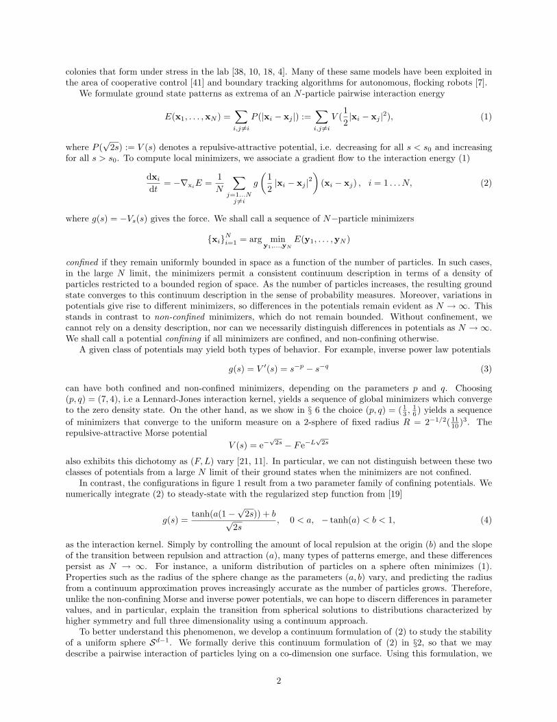
In contrast, the configurations in figure 1 result from a two parameter family of confining potentials. Wenumerically integrate (2) to steady-state with the regularized step function from [19]

g(s) =tanh(a(1−

√2s)) + b√

2s, 0 < a, − tanh(a) < b < 1, (4)

as the interaction kernel. Simply by controlling the amount of local repulsion at the origin (b) and the slopeof the transition between repulsion and attraction (a), many types of patterns emerge, and these differencespersist as N → ∞. For instance, a uniform distribution of particles on a sphere often minimizes (1).Properties such as the radius of the sphere change as the parameters (a, b) vary, and predicting the radiusfrom a continuum approximation proves increasingly accurate as the number of particles grows. Therefore,unlike the non-confining Morse and inverse power potentials, we can hope to discern differences in parametervalues, and in particular, explain the transition from spherical solutions to distributions characterized byhigher symmetry and full three dimensionality using a continuum approach.

To better understand this phenomenon, we develop a continuum formulation of (2) to study the stabilityof a uniform sphere Sd−1. We formally derive this continuum formulation of (2) in §2, so that we maydescribe a pairwise interaction of particles lying on a co-dimension one surface. Using this formulation, we

2

Figure 1: Top: Minimizers of the energy (1) with force law (4).

derive our main result in §3, that the eigenvalue problem associated to the 2-sphere of radius R reduces tothe decoupled series of 2× 2 scalar problems given by equation (30). Each eigenvalue problem determines asolution to the linearized equations in terms of spherical harmonics. We use this characterization to predicthow instabilities perturb the density away from uniform in §§3.2. We complete the eigenvalue problem forarbitrary dimensions d ≥ 2 in §4. Remarkably, the eigenvalue problem remains 2×2 and scalar independentlyof the dimension of space. Moreover, our analysis depends only on values of the potential and its derivativeson [0, 2R2]. Thus, once we know the length scale of the radius our analysis applies regardless of the far-fieldbehavior of the potential. In §5 we derive asymptotic expressions for the eigenvalues in theorem 5.1. As afirst corollary we establish the linear well-posedness of uniformly distributed sphere solutions, which servesas the analogue in our context of the classic Kelvin-Helmholtz instability for vortex sheets [20, 23, 34]. In asecond corollary, we consider potentials V with the form

− Vs(s) := g(s) =∞∑i=1

cispi , (5)

where pi < pi+1 and c1 > 0 to ensure an interaction kernel with repulsion in the short-range. We show thatonly finitely many unstable modes exist precisely when

(i)∫ 1

−1

g(R2(1− s))ds+ 4g(2R2) < 0 and (ii) p1 ∈ (−d− 12

, 0) ∪∞⋃n=0

(2n+ 1, 2n+ 2). (6)

In this case, we can predict complex patterns in the resulting ground state from the unstable sphericalharmonics. These conditions also allow us to predict the co-dimension of the ground state. We highlightthese aspects of the theory in §6 with several examples. This method also offers us a way to directly constructa potential with a specified instability which is related to the classical inverse statistical mechanics problem[9, 31, 30, 37, 13, 39]. We follow with a brief summary.

3

2 Pairwise Interactions on a Surface

We begin by formally deriving the relevant equations to describe a continuum of pairwise-interacting particleson a surface. For this, we consider the active scalar equations in three dimensions

ρt(x, t) +∇ · (ρ(x, t)u(x, t)) = 0, x ∈ R3, t ≥ 0

u(x, t) =∫

R3g(

12|x− y|2) (x− y) ρ(y, t) dy, (7)

where ρ describes the density of particles, the kernel g describes the interaction of particles, and u describesthe velocity of a particular particle due to the interaction. After constraining the density of particles to lieon a dynamically evolving surface X(ξ, η, t), where (ξ, η) lie in a Lagrangian coordinate domain D ⊂ R2, thedensity defines a distribution of the form

ρ(x, t) :=∫D

δ(x−X(ξ, η, t))f(ξ, η, t) dξdη. (8)

In other words, 〈ρ, φ〉 =∫∞

0

∫Dφ(X(ξ, η, t))f(ξ, η, t) dξdηdt holds for all test functions φ ∈ C∞0 (R3×t ≥ 0).

With a density in this form, we say (8) defines a solution to (7) in the sense of distributions. We thereforespecify equations for X and f so that∫ ∞

0

∫D

(φt + u · ∇φ)(X(ξ, η, t), t)f(ξ, η, t) dξdηdt = 0 (9)

u =∫D

g(12|x−X(ξ, η, t)|2) (x−X(ξ, η, t)) f(ξ, η, t) dξdη (10)

for all φ ∈ C∞0 .Addressing first the motion of the surface, as X(ξ, η, t) represents the position of the particle with label

(ξ, η), each point on the surface evolves according to the velocity field u at that point, so that

∂X∂t

(ξ, η, t) = u(X(ξ, η, t), t) = (11)∫D

g(12|X(ξ, η, t)−X(ξ′, η′, t)|2) (X(ξ, η, t)−X(ξ′, η′, t)) f(ξ′, η′, t) dξ′dη′.

Combining (9) and (11) with the fact that ∂∂t φ(X, t) = (φt + ∂X

∂t · ∇φ)(X, t), we discover f must satisfy∫∞0

∫D

∂∂t φ(X, t) f(ξ, η, t) dξdηdt = 0. Integrating by parts in time, this gives

∫∞0

∫Dφ(X, t)f(ξ, η, t)t dξdηdt =

0 for all φ, whence f(ξ, η, t) ≡ f(ξ, η, 0). Therefore, given an initial density

ρ(x, 0) = ρ0(x) =∫D

δ(x−X0(ξ, η))f0(ξ, η) dξdη,

by evolving the surface according to

Xt =∫D

g(12|X−X′|2) (X−X′) f0(ξ′, η′) dξ′dη′ (12)

X = X(ξ, η, t) X′ = X(ξ′, η′, t) X(ξ, η, 0) = X0(ξ, η)

we obtain a distribution solution to (7).

Remark 2.1. Equations (12) easily generalize to any dimension. We use the general d-dimensional formin §4.

Although it is superfluous for determining the evolution of the surface, it will prove useful at times tore-write (8) in a more conventional form,

ρ(x, t) :=∫D

δ(x−X)ρS(ξ, η, t)|Xξ ×Xη|(t) dξdη.

4

The auxiliary quantity ρS(ξ, η, t) then has the natural interpretation as the density of particles along thesurface. The requirement that ∂f

∂t = 0 implies the density evolves according to ∂ρS∂t = −ρS |Xξ×Xη|t

|Xξ×Xη| , whichwhen coupled to (12) becomes the extension to three dimensions of the corresponding equations from [34]for curves in two dimensions. In this manner, the evolution of the surface alone determines the density ofparticles along it; the surface X(ξ, η) is fundamental and the density is derived. For this reason, we focusour analysis on X, and use this to determine properties of ρS .

3 Eigenvalue Problem in Three Dimensions

We now determine when a sphere of uniform density defines a linearly stable solution to (12). In §§3.1, welinearize (12) about a uniform sphere, and then reduce the problem to a decoupled series of scalar eigenvalueproblems involving a single spherical harmonic. We proceed with the calculations in a manner that makesthe appearance of spherical harmonics self-evident, as the ideas behind the calculation itself prove useful forother problems. The existence of uniform sphere solutions follows as an easy application, for instance, sowe postpone it until after we derive the eigenvalue problem. In §§ 3.2, we use knowledge of the eigenvalueproblem to linearize the density ρS about the uniform distribution on the sphere. This later proves usefulfor interpreting our stability conditions in § 5, and also in § 6 for comparing our analysis against numerics.

3.1 Linearization of the Surface

We begin by considering the evolution equations for a surface (12) for the particular instance of f0 whichyields a sphere of radius R and uniform density as steady-state,

Xt =∫ π

−π

∫ π

0

g

(12|X−X′|2

)(X−X′) sin η′ dη′dξ′. (13)

Here, we parameterize a sphere of radius R as X(ξ, η) = Θ1(ξ)Θ2(η)Re1 for −π ≤ ξ ≤ π and 0 ≤ η ≤ π. The3×3 matrix Θ1 represents rotation in the y-z plane, Θ2 rotates in the x-y plane, and of course e1 = (1, 0, 0)t.

Write a perturbation δX of the steady-state in the form

δX = Θ1(ξ)Θ2(η)(Re1 + ε(ξ, η)eλt), (14)

with the goal of choosing the ansatz for ε ∈ R3 in such a way that the linear equations for ε reduce to ascalar eigenvalue problem for λ and scalar coefficients that will determine ε. First, we substitute δX into(13) and obtain

λΘ1(ξ)Θ2(η)ε(ξ, η) =∫ π

−π

∫ π

0

g

(12|δX− δX′|2

)(δX− δX′) sin η′ dη′dξ′. (15)

Decomposing δX−δX′ := X1+X2, where X1 = [Θ1(ξ)Θ2(η)−Θ1(ξ′)Θ2(η′)]Re1 and X2 = Θ1(ξ)Θ2(η)ε(ξ, η)−Θ1(ξ′)Θ2(η′)ε(ξ′, η′), we expand to first order in X2 and use the fact that the sphere is a steady-state toobtain

λΘ1(ξ)Θ2(η)ε(ξ, η) =∫ π

−π

∫ π

0

g(

12|X1|2)X2 + gs(

12|X1|2)(X1 ·X2)X1

sin η′ dη′dξ′. (16)

Denoting by M the matrix M := Θ−12 (η)Θ1(ξ′ − ξ)Θ2(η′) and by I the 3 × 3 identity matrix, simple

calculations yield

Θ−12 (η)Θ−1

1 (ξ)X1 = (I −M)Re1, Θ−12 (η)Θ−1

1 (ξ)X2 = ε(ξ, η)−Mε(ξ′, η′)

X1 ·X2 = (I −M)Re1 · ε(ξ, η) + (I −M t)Re1 · ε(ξ′, η′), |X1| = |(I −M)Re1|.

5

By premultiplying (16) with Θ−12 Θ−1

1 and separating terms involving ε(ξ, η) from terms involving ε(ξ′, η′),we obtain the linearized problem

λε(ξ, η) =∫ π

−π

∫ π

0

g(

12|v|2)I + gs(

12|v|2)v ⊗ v

ε(ξ, η) sin η′ dη′dξ′+∫ π

−π

∫ π

0

gs(

12|v|2)v ⊗ v − g(

12|v|2)M

ε(ξ′, η′) sin η′ dη′dξ′, (17)

where we define v := (I −M)Re1 and v := (I −M t)Re1.The difficulty now lies in choosing ε(ξ, η) in such a way that the continuous eigenvalue problem (17)

reduces to a simple scalar eigenvalue problem. To find the way forward, we recall the analogous situation intwo dimensions, as detailed in [19]. In that setting, the continuous eigenvalue problem reads

λε(s) =∫ π

−π

g(

12|v|2)I + gs(

12|v|2)v ⊗ v

ε(s) ds′+∫ π

−π

gs(

12|v|2)v ⊗ v − g(

12|v|2)Θ(s′ − s)

ε(s′) ds′

where v = (I − Θ(s′ − s))Re1, v = (I − Θ(s − s′))Re1 and Θ(s) denotes a 2 × 2 rotation matrix. We canwrite this as

λε(s) =∫ π

−πM1(s− s′)ε(s) ds′ +

∫ π

−πM2(s− s′)ε(s′) ds′, (18)

for some 2×2 matrices Mi. Letting M jki denote the (j, k) entry of the matrix Mi, we find that both matrices

possess even, periodic entries in s− s′ whenever j = k, and odd, periodic entries whenever j 6= k. Changingvariables (i.e. reparameterizing the circle) in the first integral, we have∫ π

−πM jki (s− s′) ds′ =

∫ π

−πM jki (θ) dθ ∝ δjk.

Thus, the first term on the RHS of (18) simplifies to a constant diagonal matrix times ε(s). We thensubstitute the known ansatz for ε from [19] into the second integral, ε(s′) = (c1 cos(ms′), c2 sin(ms′))t forsome constants c1 and c2, change variables and simplify. Along the first column of M2, we find∫ π

−πM11

2 (s− s′)c1 cos(ms′) ds′ =∫ π

−πM11

2 (θ)c1 cos(mθ +ms) dθ ∝ cos(ms) (19)

∫ π

−πM21

2 (s− s′)c1 cos(ms′) ds′ =∫ π

−πM21

2 (θ)c2 cos(mθ +ms) dθ ∝ sin(ms) (20)

due to the even-odd structure of M2. Arguing similarly along the second column, the second term on theRHS of (18) simplifies as∫ π

−πM2(s− s′)ε(s′) ds′ = D(c1, c2,m)(cos(ms), sin(ms))t,

where D denotes a constant, diagonal matrix depending upon c1, c2 and the Fourier coefficients of the entriesof M2. Moreover, D(c1, c2,m) is linear in the coefficients (c1, c2) that determine ε. As the first integral alsoresults in something of this form, the continuous problem reduces to a scalar eigenvalue problem in (c1, c2).From (20), then, we deduce the essential property of the ansatz:

∫ π−πM

ij2 (s− s′)εj(s′) ds′ ∝ εi(s).

Returning now to the three-dimensional case, regardless of the choice of the ansatz ε(ξ, η), we first mustshow the first integral in (17) yields a constant, diagonal matrix. To do this, note the integrand dependsonly upon the vector v. Looking at the definition of v, for fixed (ξ, η) and for −π ≤ ξ′ ≤ π, 0 ≤ η′ ≤ π, wesee that v simply represents a parameterization of ∂B(Re1, R), i.e. the sphere of radius R centered at thepoint (R, 0, 0)t. Moreover, |vξ′ × vη′ | = sin η′, so that by definition∫ π

−π

∫ π

0

g(

12|v|2)I + gs(

12|v|2)v ⊗ v

ε(ξ, η) sin η′ dη′dξ′ =

6

(∫∂B(Re1,R)

G(x)dS(x)

)ε(ξ, η),

where the 3 × 3 matrix valued function G(x) = g( 12 |x|

2)I + gs( 12 |x|

2)x ⊗ x for x ∈ R3. As in the two-dimensional case, we re-parameterize ∂B(Re1, R) and compute the first integral above to obtain a diagonalmatrix times ε(ξ, η). Therefore, analagous to the two-dimensional case, we should choose the ansatz forε(ξ, η) in such a way so that∫ π

−π

∫ π

0

M ij2 (ξ, ξ′, η, η′)εj(ξ′, η′) sin η′ dη′dξ′ ∝ εi(ξ, η).

Let us now turn to this task. To simplify the notation, let x := X(ξ, η) and w := X(ξ′, η′) withX(ξ, η) denoting our parameterization of the sphere. Consider the quantity x ·w := X(ξ, η) ·X(ξ′, η′). Asv = (I −M)Re1 and v = (I −M t)Re1, straightforward calculations yield

v = R

(1− x ·w,−(x ·w)η,−

(x ·w)ξsin(η)

)t|v|2 = 2R2(1− x ·w) (21)

v = R

(1− x ·w,−(x ·w)η′ ,−

(x ·w)ξ′sin(η′)

)t. (22)

We now make the key observation that M112 depends only upon the quantity x ·w, in that M11

2 (ξ, ξ′, η, η′) =g1(x ·w) for g1(s) = R2gs(R2(1 − s))(1 − s)2 − g(R2(1 − s))s. For such functions, we shall make repeateduse the following (c.f. [32]):

Theorem 3.1. (Funk-Hecke Theorem in 3D) Let f(s) ∈ L1([−1, 1]). Then for any spherical harmonic Sl(x)of degree l and x ∈ S2,

λSl(x) =∫S2f(x ·w)Sl(w) dSw. (23)

The eigenvalue λ depends only on the function f and the degree l of the harmonic, where we will now writeλ = λl(f) to make explicit the dependencies of the eigenvalues on the functions involved. More specifically,

λl(f) = 2π∫ 1

−1

f(s)Pl(s) ds, (24)

where Pl(s) denotes the Legendre polynomial of degree l, normalized to Pl(1) = 1. In three dimensions,equation (23) plays the role that equation (20) serves in two dimensions.

Together with our observation regarding M112 , this theorem suggests we choose ansatz with ε1(ξ, η) =

c1Sl(x(ξ, η)) for some coefficient c1 ∈ R. Indeed, then∫ π

−π

∫ π

0

M112 (ξ, ξ′, η, η′)ε1(ξ′, η′) sin η′ dη′dξ′ = c1

∫S2g1(x ·w)Sl(w) dSw

so that by a straightforward application of the Funk-Hecke (F-H) theorem,∫ π

−π

∫ π

0

M112 (ξ, ξ′, η, η′)ε1(ξ′, η′) sin η′ dη′dξ′ = λl(g1)c1Sl(x) ∝ ε1

as desired. With ε1 now in hand, we can use the requirement that∫ π

−π

∫ π

0

M i12 (ξ, ξ′, η, η′)ε1(ξ′, η′) sin η′ dη′dξ′ ∝ εi(ξ, η) (25)

to determine the remainder of the ansatz. For this, we observe that the relations (21) and (22) imply

M212 =

(g(

12|v|2)(1− x ·w)

)η

M312 =

1sin(η)

(g(

12|v|2)(1− x ·w)

)ξ

.

7

Using this with the known choice of ε1, we find the relation (25) for i = 2 becomes

ε2(ξ, η) ∝∫S2

(g(

12|v|2)(1− x ·w)

)η

c1Sl(w) dSw = c1

(∫S2g2(x ·w)Sl dSw

)η

,

where g2(s) = g(R2(1 − s))(1 − s), by passing the derivative through the integral in the primed variables.Again using the F-H theorem, we recover ε2(ξ, η) ∝ c1λl(g2)Slη. Arguing similarly from (25) with i = 3yields ε3(ξ, η) ∝ c1λl(g2)

sin(η) Slξ. All together, we recover

ε(ξ, η) =(c1S

l(x), c2(Sl(x))η, c3(Sl(x))ξsin(η)

)t(26)

for real coefficients ci.Proceeding as in the two-dimensional case, it remains to show that this choice of ε(ξ, η) yields∫ π

−π

∫ π

0

M2(·)ε(ξ′, η′) sin η′ dη′dξ′ = D(c1, c2, c3, l)

(Sl, Slη,

Slξsin(η)

)t,

where D(c1, c2, c3, l) is a constant, diagonal matrix that is linear in the coefficients. The derivation of theansatz has demonstrated this claim for the first column of M2. Continuing with the remainder first row ofM2, in light of (21) and (22) we see

M122 =

(g(

12|v|2)(1− x ·w)

)η′M13

2 =1

sin(η′)

(g(

12|v|2)(1− x ·w)

)ξ′.

In setting c2 = c3, we compute∫ π−π∫ π

0(M12

2 ε2 +M132 ε3) sin η′ dη′dξ′ =

c2

∫ π

−π

∫ π

0

(g2(x ·w))η′Sl(w)η′ sin η′ dη′dξ′ + c2

∫ π

−π

∫ π

0

(g2(x ·w))ξ′Slξ′sin(η′)2

sin η′ dη′dξ′.

Integrating by parts in η′ in the first term and in ξ′ in the second term, we have∫ π

−π

∫ π

0

(M122 ε2 +M13

2 ε3) sin η′ dη′dξ′ = −c2∫ π

−π

∫ π

0

(∆S2Sl)g2(x ·w) sin η′ dη′dξ′.

Using that ∆S2Sl = −l(l + 1)Sl and the F-H theorem, we obtain∫ π−π∫ π

0(M12

2 ε2 + M132 ε3) sin η′ dη′dξ′ =

c2l(l + 1)λl(g2)Sl(x) ∝ ε1 as desired. Proceeding similarly with the remainder of the second row of M2, thefacts

M222 = −(g(

12|v|2))η′(x ·w)η − g(

12|v|2)(x ·w)ηη′ ,

M232 =

−(g( 12 |v|

2))ξ′(x ·w)η − g( 12 |v|

2)(x ·w)ηξ′sin(η′)

and a similar integration by parts combine to give∫ π

−π

∫ π

0

(M222 ε2 +M23

2 ε3) sin η′ dη′dξ′ = c2

∫ π

−π

∫ π

0

g(12|v|2)(x ·w)η(∆S2Sl)dS2

= −c2l(l + 1)∫ π

−π

∫ π

0

g(12|v|2)(x ·w)ηSl(w) sin η′ dη′dξ′.

Letting g3(s) =∫ R2(1−s)

0g(z) dz, so that g3(x ·w)η = −R2g( 1

2 |v|2)(x ·w)η, we pass the derivative through

the integral and use the F-H theorem as before to arrive at∫ π

−π

∫ π

0

(M222 ε2 +M23

2 ε3) sin η′ dη′dξ′ =c2l(l + 1)λl(g3)

R2Slη ∝ ε2.

8

Finally, the same argument on the remainder of the last row of M2 gives∫ π

−π

∫ π

0

(M322 ε2 +M33

2 ε3) sin η′ dη′dξ′ =c2l(l + 1)λl(g3)

R2 sin(η)Slξ ∝ ε3.

Combining all of the above, we find∫ π

−π

∫ π

0

M2(ξ, ξ′, η, η′)ε(ξ′, η′) sin η′ dη′dξ′ =

(D11Sl, D22Slη, D

33Slξ

sin(η)

)t,

D11 = c1λl(g1) + c2l(l + 1)λl(g2)D22 = D33 = c1λl(g2) + c2l(l + 1)R2

λl(g3),

so that D is linear in the coefficients as desired. Consequently, with this ansatz the linearized equations (17)become

λε(ξ, η) =

(∫∂B(Re1,R)

G(x)dS(x)

)ε(ξ, η) +D(c1, c2, l)ε(ξ, η). (27)

By symmetry, we see (∫∂B(Re1,R)

G(x)dS(x)

)= diag(α, β, β),

so that the second and third equations in (27) are identical. Consequently, solving the continuous linearizedequations reduces to the 2× 2 scalar eigenvalue problem determined by (27): λc1 = αc1 +D11(c1, c2, l) andλc2 = βc2 +D22(c1, c2, l), just as in the two-dimensional case.

We can make one final simplification to the eigenvalue problem that comes from the steady-state equationfor the sphere,

0 =∫S2g(R2

2|x−w|2)(x−w) dSw. (28)

In particular, the sphere radius R satisfies (see Remark 3.2 below)

0 =∫S2g(R2(1− x ·w))(1− x ·w) dSy ⇔ 0 =

∫ 1

−1

g2(s)ds (29)

by the F-H theorem with l = 0. A simple calculation then gives β = 0.To summarize the previous calculations, the decoupled sequence of eigenvalue problems

λ

(c1c2

)=(α+ λl(g1) l(l + 1)λl(g2)λl(g2) l(l+1)

R2 λl(g3)

)(c1c2

):= Ωl

(c1c2

)(30)

determine the linear stability of the uniform sphere. To compute the entries of Ωl, we recall that for a functionh ∈ L1([−1, 1]) and l ∈ N we define λl(h) = 2π

∫ 1

−1h(s)Pl(s)ds, with Pl(s) denoting the Legendre polynomial

of degree l normalized to Pl(1) = 1. The radius R of the sphere satisfies 0 =∫ 1

−1g(R2(1− s))(1− s)ds and

the coefficient α = 8πg(2R2) + 2π∫ 1

−1g(R2(1− s))ds. Finally, we recall the definitions

g1(s) = R2gs(R2(1− s))(1− s)2− g(R2(1− s))s, g2(s) = g(R2(1− s))(1− s), (g3)s(s) = −R2g(R2(1− s)).(31)

Remark 3.2. For sufficiently smooth attractive-repulsive interaction kernels g, a uniform density, steady-state sphere solution to equation (13) exists if and only if −∞ ≤

∫∞0sg(s) ds < 0. Indeed, projecting the

equation of steady-state (28) onto the component normal to the sphere yields

0 =∫S2g(R2(1− x ·w))(1− x ·w) dSy ⇔ 0 =

∫ 1

−1

g2(s)ds (32)

9

by the F-H theorem with l = 0. Since g > 0 near zero, for R sufficiently small the integral on the RHS of(32) is positive. Similarly, since g < 0 away from the origin, for R large enough the integral on the RHSdecreases as R → ∞. Thus when

∫∞0sg(s) ds < 0 the RHS of (32) is negative for all sufficiently large

radii. Therefore there exists an R which identically satisfies (32). That the projection onto the tangentialcomponents satisfies (28) follows in a manner similar to the derivation of the tangential components of theansatz. This applies regardless of the stability of the sphere, and regardless of whether the potential exhibitsconfinement.

Remark 3.3. In concordence with a local notion like linear stability, all equations only involve values of thepotential V and its derivatives for values of s ∈ [0, 2R2]. In particular, once we know the radius R of thesphere, we can assign arbitrary far-field behavior to the potential without affecting the validity or applicabilityof our analysis.

3.2 Linearization of the Density

By solving the eigenvalue problem (30), our work in the previous section allows us to construct approximatesolutions to the surface equations (12) with f0(ξ, η) = sin(η), which correspond to small perturbations ofthe spherical solution. As we mentioned in §2, knowledge of the surface allows us to reconstruct the densityof particles via ρS(ξ, η, t)|Xξ ×Xη|(t) = f0(ξ, η). Therefore, a perturbation away from a sphere naturallyinduces a perturbation of the density away from uniform as well. Indeed, if we write our perturbation of thesphere as u(x, t) = Θ1(ξ)Θ2(η)(Re1 + ε(x)eλt) for x(ξ, η) ∈ S2 and ε(x) as in equation (26), we can linearizeρS = sin(η)

|uξ×uη| to find the leading order corrections to the density.To this end, define B(ξ, η) := Θ1(ξ)Θ2(η). We can then compute |uξ × uη| by using Lagrange’s identity:

|uξ × uη|2 = (uξ · uξ)(uη · uη)− (uξ · uη)2.

Computing this directly, we find

|uξ|2 = |BξRe1|2 + 2RBξe1 · (Bξε(x) + Bε(x)ξ) eλt +O(ε2)

|uη|2 = |BηRe1|2 + 2RBηe1 · (Bηε(x) + Bε(x)η) eλt +O(ε2)

uξ · uη = R2(BtηBξ)11 +O(ε). (33)

Straightforward calculations yield the required derivatives of B:

BtξBξ =

sin2(η) sin(η) cos(η) 0sin(η) cos(η) cos2(η) 0

0 0 1

BtBξ =

0 0 − sin(η)0 0 − cos(η)

sin(η) cos(η) 0

BtηBη =

1 0 00 1 00 0 0

BtBη =

0 −1 01 0 00 0 0

BtηBξ =

0 0 − cos(η)0 0 sin(η)0 0 0

. (34)

Using the relations (33) and (34) and the definition of the ansatz (26), we obtain

|uξ|2 = sin2(η)

R2 + 2Rc1eλtSl + 2Rc2eλt(cot(η)Slη +

Slξξ

sin2(η))

+O(ε2)

|uη|2 = R2 + 2Reλtc1S

l + c2Slηη

+O(ε2), (uξ · uη)2 = O(ε2).

Therefore, |uξ × uη|2 = sin2(η)R4 + 4c1eλtR3Sl + 2c2eλtR3(∆S2Sl)

+O(ε2), so that to leading order the

perturbed density ρS obeys

ρS =1R2

1− eλt

R(2c1 − c2l(l + 1))Sl(x)

+O(ε2). (35)

10

Additionally, we can determine the principal correction to the radius of the surface,

|u(x, t)| =√R2 + 2c1eλtRSl(x) +O(ε2) = R(1 +

c1eλt

RSl(x)) +O(ε2). (36)

We may therefore view the modes determined by the eigenvalue problems (30) as spheres of variable radiusR+ c1e

λtSl(x), with the non-uniform particle density determined from (35).

4 Eigenvalue Problem in Arbitrary Dimensions

In this section, we extend our analysis of the linearization of the surface equation and the reduction to ascalar eigenvalue problem to an arbitrary (d − 1)-sphere. Although the notation is more cumbersome, theargument proceeds exactly as in the three-dimensional case. Additionally, due to the tangential isotropy ofthe sphere, the matrix associated to the eigenvalue problem remains 2× 2, regardless of dimension.

In the d–dimensional setting, the analogue of (13) becomes

Xt(η1, . . . , ηd−1, t) =∫Sd−1

g(12|X−X′|2)(X−X′) dSd−1 (37)

X = X(η1, . . . , ηd−1, t) ∈ RdX′ = X(η′1, . . . , η′d−1, t) ∈ Rd,

so that a uniformly distributed steady-state sphere of radius R satisfies

0 =∫Sd−1

g(R2

2|x−w|2)(x−w) dSw ∀x ∈ Sd−1.

We write the sphere of radius R in dimension d as Rx for x ∈ Sd−1, and write a perturbation in the formδx = Rx + B(x)ε(x)eλt. The matrix B plays the role of Θ1(ξ)Θ2(η) from the three dimensional calculation,i.e. a product of rotation matrices. We define the rows bj of B(x) as follows: we take b1 = x; next,

define bj(x) = ∂ηj (x), where ηj denote any of the coordinates on Sd−1; lastly, normalize bj(x) = bj(x)

|bj(x)|.

Then BtB(x) = I for all x ∈ Sd−1. As for the ansatz, put ε1(x) = c1Sl(x) as before, and εj+1(x) =

c2∂ηj (Sl(x))/|bj(x)| for 1 ≤ j ≤ d− 1.

If we now expand to first order in ε and use the fact that the sphere is a steady-state, we obtain thecontinuous eigenvalue problem

λε(x) =∫Sd−1

g(

12|v|2)I + gs(

12|v|2)v ⊗ v

ε(x) dSw+∫

Sd−1

gs(

12|v|2)v ⊗ v − g(

12|v|2)Bt(x)B(w)

ε(w) dSw, (38)

where v = R(e1 − Bt(x)w) and v = R(e1 − Bt(w)x). This generalizes (17) to any dimension. As in threedimensions, the reduction to a scalar eigenvalue problem follows from two claims. If we let M1 denote thematrix in the first term of (38), we first claim that M1 is diagonal of the form M1 = diag(α, 0, · · · , 0) andindependent of x. Second, we claim that∫

Sd−1M2(x,w)ε(w) dSw = (D11Sl, D22

Slη1

|b1|, . . . , D22

Slηd−1

|bd−1|),

where M2 denotes the matrix in the second term of (38), and Dii = Dii(c1, c2, l) are linear in the coefficients.Combining this with the first claim again reduces (38) to the scalar eigenvalue problem

λ

(c1c2

)=(αc1 +D11(c1, c2, l)

D22(c1, c2, l)

).

To establish the claims, we once again have as our main tool ([32]):

11

Theorem 4.1. (Funk-Hecke Theorem in d-dimensions) Let f(s)(1 − s2)d−32 ∈ L1([−1, 1]). Then for any

spherical harmonic of degree l and x ∈ Sd−1,

λSl(x) =∫Sd−1

f(x ·w)Sl(w) dSw.

Again, the eigenvalue λ = λl(f) depends only on the function f and the degree l of the harmonic, in that

λl(f) = vol(Sd−2)∫ 1

−1

f(s)Pl,d(s)(1− s2)d−32 ds,

where vol(Sd−2) denotes the surface area of the d−2 sphere. Also, Pl,d(s) denotes the Gegenbauer polynomialP

(d/2−1)l (s) from [35], normalized so that Pl(1) = 1. For d = 3, these coincide the Legendre polynomials,

whereas for d = 2 we have Pl(cos(η)) = cos(lη). Under this change of variable, for d = 2, we recover preciselythe eigenvalue problem from [19]. We shall also need the following elementary lemma. For the proof, wedenote by w(η1, . . . , ηd−1) a parameterization of Sd−1 such that w = (cos η1, sin η1w) and w(η2, . . . , ηd−1)parametrizes Sd−2. We also use Einstein notation for terms involving partial derivatives.

Lemma 1. Let f(η1, . . . , ηd−1) ∈ C2 with (η1, . . . , ηd−1) denoting coordinates on Sd−1 as above. Then∂ηj

(fηj

dSw|wηj |2

)= ∆Sd−1(f)dSw.

Proof. We induct on the dimension d. When d = 2 this reads

∂ηfηdη = ∆S1(f)dη

so there is nothing to prove. Let us now write dSw = sind−2(η1)dSd−2, where dSd−2 depends only onη2, . . . , ηd−1. As |wη1 | = 1 and |wηj | = sin η1|wηj | for j > 1 we compute

∂ηj

(fηj

dSw|wηj |2

)= ∂η1

(fη1 sind−2 η1

)dSd−2 +

sind−2 η1

sin2 η1

∂ηj

(fηj

dSd−2

|wηj |2

),

= ∂η1(fη1 sind−2 η1

)dSd−2 +

sind−2 ∆Sd−2(f)dSd−2

sin2 η1

by the inductive hypothesis. However, dSd−2 = dSw sin2−d η1 so that we obtain

∂ηj

(fηj

dSw|wηj |2

)=(

sin2−d η1∂η1(fη1 sind−2 η1

)+

1sin2 η1

∆Sd−2(f))

dSw.

We recognize the expression in parentheses as ∆Sd−1(f).

Claim 1. In (38), M1 = diag(α, 0, · · · , 0) for some α ∈ R.

By the orthogonality of B we recognize the vector v as a parameterization of ∂B(Re1, R) in Rd. Thus,the first term in (38) amounts to multiplying ε(x) by constant matrix

M1 =∫∂B(Re1,R)

g(12|x|2)I + gs(

12|x|2)(x⊗ x) dSx.

Parametrize ∂B(Re1, R) by x = R(e1 − w), where w = (cos(η1), sin(η1)w) and w ∈ Rd−1 parametrizesSd−2. Then for j, k 6= 1 we have

M jk1 =

∫ π

0

∫Sd−2

g(R2(1− cos(η1)))δjk sin(η1)d−2 dη1dSd−2+

R2

∫ π

0

∫Sd−2

gs(R2(1− cos(η1)))(w · ej)(w · ek) sin(η1)d dη1dSd−2

= vol(Sd−2)δjk∫ 1

−1

g(R2(1− s))(1− s2)d−32 ds

+(∫Sd−2

xjxk dSd−2

)∫ 1

−1

R2gs(R2(1− s))(1− s2)d−12 ds.

12

By symmetry,∫Sd−2 xjxk dSd−2 = vol(Sd−2)

d−1 δjk, so that M jk1 =

δjkvol(Sd−2)∫ 1

−1

(g(R2(1− s)) +

R2

d− 1gs(R2(1− s))(1− s2)

)(1− s2)

d−32 ds

whenever j, k 6= 1. Integrating the last term by parts, we arrive at

M jk1 = δjkβ := δjkvol(Sd−2)

(∫ 1

−1

g(R2(1− s))(1− s)(1− s2)d−32 ds

)(39)

for j, k > 1. Thus, the lower (d− 1)× (d− 1) block of M1 takes the form diag(β, . . . , β), with β as in (39).However, for Rx to satisfy the equation of steady-state, we require 0 =

∫Sd−1 g(R2(1−x ·w))(1−x ·w)dSw.

Utilizing the F-H theorem with l = 0, this gives

0 =∫ 1

−1

g(R2(1− s))(1− s)(1− s2)d−32 ds, (40)

so that in fact β = 0.We now consider the remaining entries of M1. If we now let j = 1, k > 1 we have M1k

1 = Mk11

= −R2

∫ π

0

∫Sd−2

gs(R2(1− cos(η1)))(1− cos(η1))(w · ek) sin(η1)d−1 dη1dSd−2

= −R2

(∫Sd−2

xk dSd−2

)∫ 1

−1

gs(R2(1− s))(1− s)(1− s2)d−22 ds = 0.

Thus, M1 = diag(α, 0, . . . , 0) as claimed, where

α = vol(Sd−2)∫ 1

−1

(g(R2(1− s)) +R2gs(R2(1− s))(1− s)2

)(1− s2)

d−32 ds. (41)

♠

Claim 2. In (38), ∫Sd−1

M2(x,w)ε(w) dSw = (D11Sl, D22Slη1

|b1|, . . . , D22

Slηd−1

|bd−1|),

where Dii = Dii(c1, c2, l) are linear in (c1, c2).

Let x = x(η1, . . . , ηd−1) and w = w(η′1, . . . , η′d−1). We can then write the entries of v and v as

v1

R= (1− x ·w),

vj

R= −

∂ηj (x ·w)

|bj |(x),

v1

R= (1− x ·w),

vj

R= −

∂η′j (x ·w)

|bj |(w),

and the entries of M(x,w) := Bt(x)B(w) as

M11 = x ·w, M1j =∂η′j (x ·w)

|bj(w)|, Mj1 =

∂ηj (x ·w)

|bj(x)|, Mjk =

∂ηj∂η′k(x ·w)

|bj(x)||bj(w)|.

We now demonstrate the claim row-by-row, and in doing so, we use Einstein summation notation. Basedon the preceding definitions,∫

Sd−1M1j

2 εj dSw = c1

∫Sd−1

g1(x ·w)Sl(w) dSw+

c2

∫Sd−1

∂η′j (g2(x ·w)) ∂η′j (Sl(w))

dSw|bj(w)|2

, (42)

13

where g1(s) = R2gs(R2(1− s))(1− s)2 − g(R2(1− s))s and g2(s) = g(R2(1− s))(1− s). For the first termin (42), we use a straightforward application of the F-H theorem to obtain

c1

∫Sd−1

g1(x ·w)Sl(w) dSw = c1λl(g1)Sl(x).

We then integrate the second term in (42) by parts to obtain∫Sd−1

M1j2 εj dSw = c1λl(g1)Sl(x)− c2

∫Sd−1

g2(x ·w)∂η′j

(∂η′j (Sl(w))

dSw|bj(w)|2

). (43)

Using the lemma with f = Sl(w), (43) simplifies to∫Sd−1

M1j2 εj dSw = c1λl(g1)Sl(x)− c2

∫Sd−1

g2(x ·w)∆Sd−1(Sl(w)) dSw

= (c1λl(g1) + c2l(l + d− 2)λl(g2))Sl(x), (44)

as Sl is an eigenfunction with eigenvalue −l(l + d− 2) and the F-H theorem. This establishes the claim forthe first row with D11(c1, c2, l) = c1λl(g1) + c2l(l + d− 2)λl(g2).

Finally, we proceed to the remaining d− 1 rows. We have∫Sd−1

M jk2 εk dSw =

c1

|bj(x)|

∫Sd−1

∂ηj (g2(x ·w))Sl(w) dSw+

c2

|bj(x)|

∫Sd−1

[−g(R2(1− x ·w))η′k(x ·w)ηj−

g(R2(1− x ·w))(x ·w)ηjη′k

] ∂η′kSl(w)

|bk(w)|2dSw. (45)

In the first term of the RHS of (45), as the integral is in the η′ variables, we may pass the derivative throughthe integral to obtain

c1

|bj(x)|

∫Sd−1

∂ηj (g2(x ·w))Sl(w) dSw =c1λl(g2)∂ηjS

l(x)

|bj(x)|.

Integrating the second term of (45) by parts cancels the third term, leaving∫Sd−1

M jk2 εk dSw =

c1λl(g2)∂ηjSl(x)

|bj(x)|+

c2

|bj(x)|

∫Sd−1

g(R2(1− x ·w))(x ·w)ηj∂η′k

(∂η′kSl(w)

|bk(w)|2dSw

)

=c1λl(g2)∂ηjS

l(x)

|bj(x)|− c2l(l + d− 2)

|bj(x)|

∫Sd−1

g(R2(1− x ·w))(x ·w)ηjSl(w) dSw

using lemma 1 and the fact that Sl is an eigenfunction. If we once again let g3(s) =∫ R2(1−s)

0g(z)dz , we

may pass the derivative through the integral as before to obtain∫Sd−1

M jk2 εk dSw =

(c1λl(g2) +

c2l(l + d− 2)R2

λl(g3))∂ηjS

l(x)

|bj(x)|.

This establishes the claim in the remaining rows with D22(c1, c2, l) = c1λl(g2) + c2l(l+d−2)R2 λl(g3).

♠

14

In summary, the continuous, d-dimensional eigenvalue problem (38) reduces to the 2×2 scalar eigenvalueproblem

λ

(c1c2

)=(α+ λl(g1) l(l + d− 2)λl(g2)λl(g2) l(l + d− 2)λl(g3)

R2

)(c1c2

):= Ωl

(c1c2

)(46)

where the gi remain as in the three dimensional case.

5 Linear Stability and Linear Well-Posedness

By reducing the linearized equations to a series of scalar problems, we can now readily identify the eigenvaluesω1,2l of the matrix Ωl. This then allows us to characterize the linear stability of sphere solutions: we needω1,2l < 0 for all l ≥ 2, together with ω1

0 < 0, ω20 = 0, ω1

1 < 0 and ω21 = 0 (rotation invariance manifests as a

zero eigenvalue when l = 0, translation invariance manifests as a zero eigenvalue for l = 1). Therefore, thesphere is linearly stable if tr(Ωl) < 0 and det(Ωl) > 0 for all l ≥ 2. Due to the form of Ωl, we see det(Ωl) > 0can happen only if α+λl(g1) and λl(g3) have the same sign. The condition tr(Ωl) then forces the negativityof both, so that we deduce the stability of mode l occurs when

(i) α+ λl(g1) < 0 (ii) λl(g3) < 0 (47)

(iii) (α+ λl(g1))λl(g3) > R2[λl(g2)]2. (48)

This characterization of stability proves most useful in our analysis, and provides some additional insights.Indeed, from the relation for the perturbed density (35) and the perturbed radius (36), we see that aperturbation for which c1 = 0 corresponds to a perturbation of density along the sphere, and not of thesphere itself. Condition (ii) therefore has a natural interpretation in terms of stability of the sphere withrespect to perturbations of the density away from uniform. More specifically, as (g3)s(s) = −R2g(R2(1−s)),the function V (s) := −g3(1− s/R2) gives the potential that governs the pairwise interaction. We can thenconsider the potential energy E(ρS) of the system as a function of the density,

E(ρS) =∫S2×S2

V (12|x−w|2)ρS(x)ρS(w) dSxdSw, (49)

and ask when ρS ≡ 1 corresponds to a minimum of (49). Using the F-H theorem as in §3.1 we find thatthis happens precisely when (ii) holds for all l ≥ 1. Conversely, perturbations for which c2 = 0 have nocomponent tangential to the sphere. This happens when l = 0 for instance. In this case (48) reduces toα+λ0(g1) < 0, which gives stability of the sphere with respect to pure dilations. Condition (i), then, enforcesstability of the sphere with respect to purely normal modes.

Having characterized stability for finite l, we now wish to investigate the behavior of the spectrum asl → ∞. The most classical question concerns the linear well-posedness of sphere solutions, i.e. whenthe eigenvalues remain bounded as l → ∞. In practice, however, we primarily concern ourselves with astronger notion: we wish to characterize when the sphere is eventually stable, that is, when ω1,2

l < 0 forall l sufficiently large. With eventually stable potentials we find that the finite number of unstable modescompletely characterizes the ground state. We now address both issues using theorem 5.1, which furnishesasymptotic formulae for ω1,2

l for sufficiently regular potentials.To include the types of potentials that frequently occur in applications, we will assume V ∈ C2((0,∞)),

but allow growth in V as s → 0. Specifically, we assume V, Vs = o(s1−d2 ) as s → 0. Additionally, to

guarantee that λl(gi) are well-defined and to satisfy the hypothesis in the F-H theorem, we must requiregi(s)(1− s2)

d−32 ∈ L1([−1, 1]). Recalling from (31) that

g1(s) = R2gs(R2(1− s))(1− s)2− sg(R2(1− s)), g2(s) = g(R2(1− s))(1− s), (g3)s(s) = −R2g(R2(1− s)),

we should at least require gs(R2(1− s))(1− s)2(1− s2)d−32 , g(R2(1− s))(1− s2)

d−32 ∈ L1. We shall actually

assume slightly more, namely that

gs(R2(1− s))(1− s)(1− s2)d−32 ∈ L1, g(R2(1− s))(1− s2)

d−32 ∈ L1. (50)

Under these hypotheses, we have the following:

15

Theorem 5.1. Let V ∈ C2((0,∞)) and V, Vs = o(s1−d2 ) as s ↓ 0. Assume also (50). Then we have

(i) tr(Ωl) ∼ α and det(Ωl) ∼ R2l(l + d− 2)αλl(g3) = o(1) as l→∞.

(ii) The sphere solution of radius R given by (32) is linearly well-posed, i.e. ∃C such that ω1,2l < C for all

l ≥ 0.

(iii) Suppose g(s) has a generalized power series expansion

g(s) =∞∑i=1

cispi , p1 < p2 < · · · with c1 > 0, (51)

that converges sufficiently rapidly. If the following conditions hold

(1) α < 0 and (2) p1 ∈ (−d− 12

, 0) ∪∞⋃n=0

(2n+ 1, 2n+ 2), (52)

then the sphere is eventually stable i.e. (ii) holds for C = 0.

Remark 5.2. The condition α < 0 enforces stability with respect to high-mode normal perturbations. Indeed,when α > 0 then all sufficiently high modes have a positive eigenvalue uniformly bounded away from zero, andthe corresponding eigenfunction tends to a purely normal perturbation. Additionally, while the generalizedpower series (51) covers many potentials that occur in practice, such as the Morse potential, Gaussianpotentials and power-law potentials, the conclusion of part (iii) holds for other classes of potentials withoutsuch an expansion. For instance, if the interaction kernel grows sufficiently rapidly near the origin whileremaining smooth otherwise, part (iii) still holds. We conjecture (iii) still holds even if an expansion (51)only holds locally near zero, such as with the interaction (4).

Proof. To show (i), we need to estimate rate of decay of λl(gi). We recall that

λl(gi) = C(d)∫ 1

−1

gi(s)Pl,d(s)(1− s2)d−32 ds,

where the constant C(d) depends only on the dimension of space, d, and that the polynomial Pl,d(s) satisfiesthe Gegenbauer equation

(1− s2)P ′′l,d − (d− 1)sP ′l,d + l(l + d− 2)Pl,d = 0 (53)

together with the normalization Pl,d(1) = 1. From these definitions, we have that f(s)(1 − s2)d−32 ∈

L1([−1, 1]) guarantees λl(f) = o(1) (c.f. [14]).Consider first λl(g1). The assumptions in (50) then suffice to have g1(s)(1 − s2)

d−32 ∈ L1, so that

λl(g1) = o(1). Proceeding now to λl(g2), we have,

l(l + d− 2)λl(g2) =∫ 1

−1

g2(s)(1− s2)d−32 l(l + d− 2)Pl(s) ds =

−∫ 1

−1

g2(s)(1− s2)d−12 P ′′l,d ds+ (d− 1)

∫ 1

−1

sP ′l,d(s)(1− s2)d−32 g2(s) ds

as Pl,d satisfies the Gegenbauer equation (53). We integrate by parts in the first term, where the boundaryterms vanish due to the growth assumption on g = −Vs. The identity (s2 − 1)P ′l,d = l [sPl,d(s)− Pl−1,d(s)](equation (4.7.27) in [35]) then yields

l(l + d− 2)λl(g2) =∫ 1

−1

(g2)s(s)(1− s2)d−12 P ′l,d(s) ds

= l

∫ 1

−1

(g2)s(s)(1− s2)d−32 [Pl−1,d(s)− sPl,d(s)] ds.

16

As (g2)s(s) = −R2gs(R2(1−s))(1−s)−g(R2(1−s)), once again (50) suffices to have (l+d−2)λl(g2) = o(1),so that λl(g2) = o(l−1). Similarly, for λl(g3) we compute

l(l + d− 2)λl(g3) =∫ 1

−1

g3(s)(1− s2)d−32 l(l + d− 2)Pl,d(s) ds

= −∫ 1

−1

g3(s)(1− s2)d−12 P ′′l,d ds+ (d− 1)

∫ 1

−1

sP ′l,d(s)(1− s2)d−32 g3(s) ds.

We integrate by parts twice, where the boundary terms vanish as before, and use that (g3)s(s) = −R2g(R2(1−s)) to discover

1R2

l(l + d− 2)λl(g3) =∫ 1

−1

dds

g(R2(1− s))(1− s2)

d−12

Pl,d(s) ds.

Expanding the right hand side,

1R2

l(l + d− 2)λl(g3) = −∫ 1

−1

R2gs(R2(1− s))(1− s2) +

(d− 1)sg(R2(1− s))

(1− s2)d−32 Pl,d(s) ds.

Again (50) allows us to conclude that the first and second terms vanish as l→∞. Therefore, λl(g3) = o(l−2).As λl(g1) = o(1), λl(g3) = o(l−2) and tr(Ωl) = α + λl(g1) + l(l + d − 2)λl(g3)R−2 from (46), we have

tr(Ωl)→ α. As for det(Ωl), we have det(Ωl)R2l(l+d−2) = αλl(g3)+λl(g3)λl(g1)− [λl(g2)]2 . To discover the principal

term, we note first that λl(g3)λl(g1) clearly vanishes faster than αλl(g3). Returning to λl(g3), we integrateby parts once and again use the identity (s2 − 1)P ′l,d = l [sPl,d(s)− Pl−1,d(s)] to find

(l + d− 2)λl(g3) =∫ 1

−1

g(R2(1− s))(1− s2)d−32 [sPl,d(s)− Pl−1,d(s)] ds.

As g2(s) = g(R2(1− s))(1− s), this reads

(l + d− 2)λl(g3) = −λl(g2)− λl−1(g2)+∫ 1

−1

g(R2(1− s))(1− s2)d−32 [Pl,d(s)− sPl−1,d(s)] ds.

In particular, λl(g3) decays no faster than λl(g2)/(l + d− 2). Since λl(g2) = o(l−1), [λl(g2)]2 decays faster.In other words,

det(Ωl)R2l(l + d− 2)

= αλl(g3) + higher order terms. (54)

This concludes the proof of (i) and (ii). To show (iii), note that (g3)s(s) = −R2g(R2(1− s)). By lemma 5.3shown below, we then obtain

λl(g3) ∼ C(p1, d, R)sin(πp1)c1

1 + p1Γ(2 + p1)l−(2p1+d+1) as l→∞

where C denotes a positive constant. Thus λl(g3) < 0 for sufficiently large l as long as p1 satisfies (52). Inconjunction with α < 0 and (54), it then immediately follows tr(Ωl) < 0 and det(Ωl) > 0 for all l sufficientlylarge, so the sphere is eventually stable. This concludes the proof.

Finally, we provide the lemma which was key in deriving part (iii) of Theorem 5.1; it will also proveuseful in §6 for constructing potentials with specified instabilities.

Lemma 5.3. Let p+ d−12 > 0. Then we have

λl((1− s)p) = −2p+d−2 vol(Sd−1) sin(πp)Γ(p+ d−12 )Γ(p+ 1)Γ(d−1

2 )Γ(l − p)πΓ(l + p+ d− 1)

,

17

λl((1− s)p) ∼ −2p+d−2

πvol(Sd−1) sin(πp)Γ(p+

d− 12

)Γ(p+ 1)Γ(d− 1

2)l−2p−d+1

as l→∞.

Proof. Using the expression of Gegenbauer polynomials in terms of hypergeometric functions [35], we maywrite

λl((1− s)p)vol(Sd−1)

=∫ 1

−1

(1− s)p+(d−3)/2(1 + s)(d−3)/22F1

(−l, l + d− 2;

d− 12

;1− s

2

)ds

= 2p+d−2

∫ 1

0

tp+(d−3)/2(1− t)(d−3)/22F1

(−l, l + d− 2;

d− 12

; t)

dt

after the change of variables t = 1−s2 . The generalized Euler transform for hypergeometric functions [33]

then gives λl((1−s)p)vol(Sd−1)

=

2p+d−2B(p+d− 1

2,d− 1

2) 3F2

(−l, l + d− 2, p+

d− 12

;d− 1

2, p+ d− 1; 1

).

Using Saalschutz’s theorem [5] to evaluate the hypergeometric term, we obtain

λl((1− s)p)vol(Sd−1)

= 2p+d−2B(p+d− 1

2,d− 1

2)

Γ(l − p)Γ(p+ d− 1)Γ(−p)Γ(l + p+ d− 1)

.

Using the identity Γ(1 − z)Γ(z) = π/ sin(πz) and expanding the beta function, we arrive at the statedexpression,

πλl((1− s)p)vol(Sd−1)

= −2p+d−2 sin(πp)Γ(p+d− 1

2)Γ(p+ 1)Γ(

d− 12

)Γ(l − p)

Γ(l + p+ d− 1). (55)

For the asymptotics as l → ∞, we note that Stirling’s approximation gives Γ(l − p)/Γ(l + p + d − 1) ∼l−2p−d+1.

6 Numerical Examples

In this section, we provide numerical examples to illustrate how the different types of instability manifestas different qualitative behaviors of the ground states. We compute steady-state solutions to (2) for severaldifferent interactions g using a fourth-order Adams-Bashforth scheme, with the number of particlesN = 1000.We take random initial conditions in all cases, and simulate until the l∞ norm of (2) falls below .001/N .

We begin by considering a generalized Lennard-Jones interaction, g(s) = s−p − s−q for 0 < p, q < 1. Toensure a physically realistic potential consisting of short-range repulsion and far-field attraction, we mustdemand p > q. We then find, by (52) (ii), that λl(g3) < 0 for all but finitely many l with no furtherrestriction. The sign of α, then, completely determines the high-mode behavior. Direct computation showsthat (2R2)p−q = 2−q

2−p , so that the condition q < 2p−12p−2 determines when α < 0, and thus the eventual stability

of the sphere. To illustrate both cases, we first select (p, q) = ( 13 ,

16 ) so that α < 0. By repeatedly using

lemma 5.3, we additionally verify that for all l the stability conditions (48) hold. We therefore expect toaccurately describe the solution as a sphere of radius R = 2−1/2( 11

10 )3. Figure 2 (a) shows the resultingparticle simulation. We next select (p, q) = (1/2, 1/4), so that α > 0 and we no longer expect the solutionto concentrate on a co-dimension one manifold. As figure 2 (b) indicates, the solution instead fills a ballsurrounding the origin; the color of a particle indicates its distance to the origin.

A more interesting picture begins to emerge when the sphere destabilizes yet remains eventually stable.As our examples will illustrate, the low mode instabilities fully describe the ground state. Due to theintricate steady-states it produces, cf. figure (1), we illustrate this phenomenon with the interaction g(s) =tanh(a(1−

√2s))+b√

2sintroduced in [19]. The top of figure 3(a) depicts a computed steady-state of (2) with

(a, b) = (7,−.9). These parameters result in a mode l = 3 instability. We then compute the eigenvector(c1, c2) of Ω3, and use the result to construct the resulting surface from equation (36) and its corresponding

18

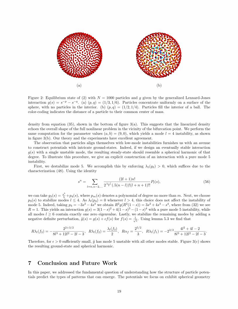
(a) (b)

Figure 2: Equilibrium state of (2) with N = 1000 particles and g given by the generalized Lennard-Jonesinteraction g(s) = s−p − s−q. (a) (p, q) = (1/3, 1/6). Particles concentrate uniformly on a surface of thesphere, with no particles in the interior. (b) (p, q) = (1/2, 1/4). Particles fill the interior of a ball. Thecolor-coding indicates the distance of a particle to their common center of mass.

density from equation (35), shown in the bottom of figure 3(a). This suggests that the linearized densityechoes the overall shape of the full nonlinear problem in the vicinity of the bifurcation point. We perform thesame computation for the parameter values (a, b) = (9, 0), which yields a mode l = 4 instability, as shownin figure 3(b). Our theory and the experiments have excellent agreement.

The observation that particles align themselves with low-mode instabilities furnishes us with an avenueto construct potentials with intricate ground-states. Indeed, if we design an eventually stable interactiong(s) with a single unstable mode, the resulting steady-state should resemble a spherical harmonic of thatdegree. To illustrate this procedure, we give an explicit construction of an interaction with a pure mode 5instability.

First, we destabilize mode 5. We accomplish this by enforcing λ5(g3) > 0, which suffices due to thecharacterization (48). Using the identity

sn =∑

l=n,n−2,...

(2l + 1)n!

2n−l2 (.5(n− l))!(l + n+ 1)!!

Pl(s), (56)

we can take g3(s) = s5

5 +p4(s), where pm(s) denotes a polynomial of degree no more than m. Next, we choosep3(s) to stabilize modes l ≤ 4. As λl(p4) = 0 whenever l > 4, this choice does not affect the instability ofmode 5. Indeed, taking p3 = −3s2− 4s3 we obtain R2g(R2(1− s)) = 3s2 + 4s3− s4, where from (32) we seeR = 1. This yields an interaction g(s) = 3(1− s)2 + 4(1− s)3− (1− s)4 with a pure mode 5 instability, whileall modes l ≥ 6 contain exactly one zero eigenvalue. Lastly, we stabilize the remaining modes by adding anegative definite perturbation, g(s) = g(s) + εf(s) for f(s) = 1√

s. Using lemma 5.3 we find that

Rλl(f3) = − 22+3/2

8l3 + 12l2 − 2l − 3, Rλl(f2) =

λl(f3)2

, Rαf =25/2

3, Rλl(f1) = −23/2 4l2 + 4l − 2

8l3 + 12l2 − 2l − 3.

Therefore, for ε > 0 sufficiently small, g has mode 5 unstable with all other modes stable. Figure 3(c) showsthe resulting ground-state and spherical harmonic.

7 Conclusion and Future Work

In this paper, we addressed the fundamental question of understanding how the structure of particle poten-tials predict the types of patterns that can emerge. The potentials we focus on exhibit spherical geometry

19

(a) (b) (c)

Figure 3: Top row: The result of the simulation of the gradient flow (2) with N = 1000 particles for threedifferent force laws. Bottom row: linearized solution corresponding to the instability mode as computed from(30). (a) Top: force law (4) with (a, b) = (7,−.9). Bottom: Perturbation of a sphere using the sphericalharmonic of mode l = 3,m = 2. (b) Top: Same as (a) but with (a, b) = (9, 0). Bottom: Perturbation ofa sphere using the spherical harmonic of mode l = 4,m = 0. (c) Top: g(s) = 3(1 − s)2 + 4(1 − s)3 − (1 −s)4 + εs−1/2 with ε = 2−3/2. Sphere perturbed by a linear combination of the modes l = 5,m = 5 andl = 5,m = 0. The figures are color-coded according to the distance from the origin.

but solutions may form into both co-dimension one and co-dimension zero patterns. We analyzed this be-havior by considering the linear stability of uniform sphere solutions to the equations governing a continuumof pairwise interacting particles on a surface. We reduced the d-dimensional eigenvalue problem into a de-coupled series of 2 × 2 scalar problem involving a single spherical harmonic. This reduction allowed us toformulate stability and linear well-posedness conditions that have natural physical interpretations. Theseconditions provide us with a means to predict the co-dimension and the types of symmetries that will emergein the resulting patterns. Using this predictive ability, we explicitly constructed a potential to yield a desiredparticle distribution, thereby addressing a particular case of the inverse statistical mechanics problem forself-assembly. In a subsequent paper, we extend this construction to arbitrary instabilities. Also, we notethat our theory currently allows us to predict only the degree of a spherical harmonic that appears in theground state. In dimensions d ≥ 3, it remains an open issue to determine which spherical harmonic of aparticular degree will arise. We plan to address this in future work.

8 Acknowledgements

We would like thank Andrew Bernoff for helpful conversations about this project. DU was partially fundedby the UC President’s Fellowship and NSF DMS-0902792. ALB acknowledges funding from NSF grantsEFRI-1024765 and DMS-0907931, as well as ONR grant N000141010641. TK is supported by NSERC grant47050.

20

References

[1] Eric L. Altschuler, Timothy J. Williams, Edward R. Ratner, Robert Tipton, Richard Stong, FaridDowla, and Frederick Wooten. Possible global minimum lattice configurations for thomson’s problemof charges on a sphere. Phys. Rev. Lett., 78(14):2681–2685, Apr 1997.

[2] Anna M. Barry, Glen R. Hall, and C. Eugene Wayne. Relative Equilibria of the (1+N)-Vortex Problem.arXiv, 1012.1002v1, 2010.

[3] A.J. Bernoff and C.M. Topaz. A primer of swarm equilibria. arXiv, 1008.0881v1, 2010.

[4] Michael P. Brenner, Peter Constantin, Leo P. Kadanoff, Alain Schenkel, and Shankar C. Venkataramani.Diffusion, attraction and collapse. Nonlinearity, 12(4):1071, 1999.

[5] J.L. Burchnall and A. Lakin. The theorems of Saalschutz and Dougall. Quart. J. Math., 2(1), 1950.

[6] Scott Camazine, Jean-Louis Deneubourg, Nigel R. Franks, James Sneyd, Guy Theraulaz, and EricBonabeau. Self-Organization in Biological Systems. Princeton Univ. Press, Princeton, 2003.

[7] Yao-Li Chuang, Y.R. Huang, M.R. D’Orsogna, and A.L. Bertozzi. Multi-vehicle flocking: Scalabilityof cooperative control algorithms using pairwise potentials. In Robotics and Automation, 2007 IEEEInternational Conference on, pages 2292 –2299, 2007.

[8] Henry Cohn and Abhinav Kumar. Universally optimal distribution of points on spheres. J. Amer.Math. Soc., 20(1):99–148, 2007.

[9] Henry Cohn and Abhinav Kumar. Algorithmic design of self-assembling structures. PNAS,106(24):9570–9575, 2009.

[10] Anna M. Delprato, Azadeh Samadani, A. Kudrolli, and L. S. Tsimring. Swarming ring patterns inbacterial colonies exposed to ultraviolet radiation. Phys. Rev. Lett., 87(15):158102, Sep 2001.

[11] M. R. D’Orsogna, Y. L. Chuang, A. L. Bertozzi, and L. S. Chayes. Self-propelled particles with soft-coreinteractions: Patterns, stability, and collapse. Phys. Rev. Lett., 96(10):104302, Mar 2006.

[12] Leah Edelstein-Keshet, James Watmough, and Daniel Grunbaum. Do travelling band solutions describecohesive swarms? An investigation for migratory locusts. Journal of Mathematical Biology, 36:515–549,1998. 10.1007/s002850050112.

[13] Szilard N. Fejer, Tim R. James, Javier Hernandez-Rojas, and David J. Wales. Energy landscapes forshells assembled from pentagonal and hexagonal pyramids. Phys. Chem. Chem. Phys., 11:2098–2104,2009.

[14] George Gasper and Walter Trebels. A Riemann-Lebesgue lemma for Jacobi expansions. In A.I. ZayedM.E.H. Ismail, M.Z. Nashed and A.F. Gholeb, editors, Mathematical Analysis, Wavelets, and SignalProcessing: an international conference on mathematical analysis and signal processes, volume 90 ofContemporary Mathematics. Amer. Math. Soc., Providence, R.I., 1995.

[15] N. R. Franks I. D. Couzin, J. Krauss and S. A. Levin. Effective leadership and decision-making inanimal groups on the move. Nature, 433:513–516, 2005.

[16] Mohamed I. Jamaloodeen and Paul K. Newton. The N -vortex problem on a rotating sphere. II. het-erogeneous platonic solid equilibria. Proc. R. Soc. A, 462(2075):3277–3299, 2008.

[17] S. A. Kaufmann. The Origins of Order: Self-Organization and Selection in Evolution. Oxford UniversityPress, New York, 1933.

[18] Evelyn F. Keller and Lee A. Segel. Model for chemotaxis. Journal of Theoretical Biology, 30(2):225 –234, 1971.

21

[19] Theodore Kolokolnikov, Hui Sun, David Uminsky, and Andrea L. Bertozzi. A theory of complex patternsarising from 2D particle interactions. Submitted.

[20] Robert Krasny. A study of singularity formation in a vortex sheet by the point-vortex approximation.J. Fluid Mech., 167:65–93, 1986.

[21] Andrew J. Leverentz, Chad M. Topaz, and Andrew J. Bernoff. Asymptotic dynamics of attractive-repulsive swarms. SIAM Journal on Applied Dynamical Systems, 8:880–908, 2009.

[22] Ryan Lukemana, Yue-Xian Lib, and Leah Edelstein-Keshet. Inferring individual rules from collectivebehavior. PNAS, 10(107), 2010.

[23] Andrew Majda and Andrea Bertozzi. Vorticity and Incompressible Flow. Cambridge University Press,2002.

[24] A. Mogilner, L. Edelstein-Keshet, L. Bent, and A. Spiros. Mutual interactions, potentials, and individualdistance in a social aggregation. Journal of Mathematical Biology, 47:353–389, 2003. 10.1007/s00285-003-0209-7.

[25] Paul K. Newton and Takashi Sakajo. The N -vortex problem on a rotating sphere. III. ring configurationscoupled to a background field. Proc. R. Soc. A, 463(2080):961–977, 2007.

[26] Paul K. Newton and Takashi Sakajo. Point vortex equilibria and optimal packings of circles on a sphere.Proc. R. Soc. A, 2010.

[27] J. K. Parrish and L. Edelstein-Keshet. Complexity, Pattern, and Evolutionary Trade-Offs in AnimalAggregation. Science, 284(99), 1999.

[28] A. Perez-Garrido, M. J. W. Dodgson, and M. A. Moore. Influence of dislocations in thomson’s problem.Phys. Rev. B, 56(7):3640–3643, Aug 1997.

[29] I. Prigogine. Order Out of Chaos. Bantam, New York, 1984.

[30] Mikael Rechtsman, Frank Stillinger, and Salvatore Torquato. Designed interaction potentials via inversemethods for self-assembly. Phys. Rev. E, 73(1):011406, Jan 2006.

[31] Mikael C. Rechtsman, Frank H. Stillinger, and Salvatore Torquato. Optimized interactions for targetedself-assembly: Application to a honeycomb lattice. Phys. Rev. Lett., 95(22):228301, Nov 2005.

[32] R.T. Seeley. Spherical harmonics. The American Mathematical Monthly, 73(4), 1966.

[33] L.J. Slater. Generalized hypergeometric functions. Cambridge University Press, 1966.

[34] Hui Sun, David Uminsky, and Andrea L. Bertozzi. A generalized Birkhoff-Rott equation for 2D activescalar problems. submitted, 2010.

[35] G. Szego. Orthogonal Polynomials. Amer. Math. Soc., Providence, RI, 4th edition, 1975.

[36] Chad M. Topaz and Andrea L. Bertozzi. Swarming patterns in a two-dimensional kinematic model forbiological groups. SIAM Journal on Applied Mathematics, 65(1):152–174, 2004.

[37] Salvatore Torquato. Inverse optimization techniques for targeted self-assembly. Soft Matter, 5:1157–1173, 2009.

[38] Lev Tsimring, Herbert Levine, Igor Aranson, Eshel Ben-Jacob, Inon Cohen, Ofer Shochet, andWilliam N. Reynolds. Aggregation patterns in stressed bacteria. Phys. Rev. Lett., 75(9):1859–1862,Aug 1995.

[39] David J. Wales. Energy landscapes of clusters bound by short-ranged potentials. Chem. Eur. J. ofChem. Phys., 11(12):2491–2494.

22

[40] McKay Hayley Wales, David J. and Eric L. Altschuler. Defect motifs for spherical topologies. Phys.Rev. B, 79(22):224115, Jun 2009.

[41] Wen Yang, A.L. Bertozzi, and Xiaofan Wang. Stability of a second order consensus algorithm with timedelay. In Decision and Control, 2008. CDC 2008. 47th IEEE Conference on, pages 2926 –2931, 2008.

23