Predicting Output Performance of a Petascale Supercomputer

Bing XieDuke University

bingxie@cs.duke.edu

Yezhou HuangDuke University

yhuang@cs.duke.edu

Jefrey S. ChaseDuke University

chase@cs.duke.edu

Jong Youl ChoiOak Ridge National Laboratory

choij@ornl.gov

Scott KlaskyOak Ridge National Laboratory

klasky@ornl.gov

Jay LofsteadSandia National Laboratories

glofst@sandia.gov

Sarp OralOak Ridge National Laboratory

oralhs@ornl.gov

ABSTRACT

In this paper, we develop a predictive model useful for output perfor-

mance prediction of supercomputer ile systems under production

load. Our target environment is TitanÐthe 3rd fastest supercom-

puter in the worldÐand its Lustre-based multi-stage write path.

We observe from Titan that although output performance is highly

variable at small time scales, the mean performance is stable and

consistent over typical application run times. Moreover, we ind

that output performance is non-linearly related to its correlated pa-

rameters due to interference and saturation on individual stages on

the path. These observations enable us to build a predictive model

of expected write times of output patterns and I/O conigurations,

using feature transformations to capture non-linear relationships.

We identify the candidate features based on the structure of the

Lustre/Titan write path, and use feature transformation functions

to produce a model space with 135,000 candidate models. By search-

ing for the minimal mean square error in this space we identify a

good model and show that it is efective.

KEYWORDS

Petascale supercomputer, Output performance, Linear regression

1 INTRODUCTION

Supercomputers and their I/O systems are built to host HPC (High

Performance Computing) applications. These applications perform

a variety of analyses, experiments and simulations [4ś7, 19] from

diferent scientiic domains. Typical HPC applications issue peri-

odic bursts of output to the ile system for intermediate results and

checkpointing; these outputs may total a terabyte or more over a

typical run of the application [4, 5, 7, 21]. US-DOE (Department of

Energy) leadership computing facilities report that HPC applica-

tions generate hundreds of petabytes of science data per year and

ACM acknowledges that this contribution was authored or co-authored by an em-ployee, or contractor of the national government. As such, the Government retains anonexclusive, royalty-free right to publish or reproduce this article, or to allow othersto do so, for Government purposes only. Permission to make digital or hard copies forpersonal or classroom use is granted. Copies must bear this notice and the full citationon the irst page. Copyrights for components of this work owned by others than ACMmust be honored. To copy otherwise, distribute, republish, or post, requires priorspeciic permission and/or a fee. Request permissions from permissions@acm.org.

HPDC’17, June 26-30, 2017, Washington, DC, USA

© 2017 ACM. 978-1-4503-4699-3/17/06. . . $15.00DOI: http://dx.doi.org/10.1145/3078597.3078614

estimate that this rate will exceed an exabyte per year by 2018 [16].

Trends suggest that HPC applications are likely to generate more

and larger output bursts.

Consequently, understanding performance of output burst ab-

sorption is crucial for these codes. Many HPC applications are

loosely synchronous or bulk synchronous: they execute a sequence

of iterations (e.g., for simulation timesteps) interspersed by barri-

ers. These applications often initiate a synchronous output burst

between iterations, and then wait for the burst to complete before

resuming computation for the next iteration. This pause provides a

consistent output image for checkpoints, and in certain other cases

when double-bufering requires too much memory to be practical.

Therefore, CPUs are left idle during the synchronous burst. As a

case study we consider XGC [5], an important code that simulates

magnetic coninement of plasma in future fusion reactor designs

(ğ2.1). In practice output times typically comprise 7-20% of XGC’s

total (wall clock) execution time.

The HPC community recognizes the importance of I/O output

performance. There are many eforts to address it. For example, [3,

26] summarize I/O access patterns across scientiic domains and su-

percomputing platforms; [22, 25, 40] investigate behaviors of petas-

cale ile systems under various access patterns and system condi-

tions. Others propose techniques, tools and middleware systems to

improve I/O performance by reducing metadata operations [23, 33],

aggregating/striping/reordering data streams [8, 16, 20, 24], and

other techniques [13, 32, 35]. These works on I/O performance

range from quantitative analysis on various targets to optimization

techniques at various levels.

This paper presents an analysis to derive principles from quanti-

tative models and to specify tradeofs of techniques across settings

and conditions. A key obstacle to meeting this goal is the dynamic

nature of our production supercomputer environment. Applica-

tions have full ownership of the compute nodes assigned to them,

but the interconnect and I/O system are shared and provide no

performance isolation. The resulting noise complicates the task of

modeling or predicting I/O performance.

We report observations from Titan [13]Ða production supercom-

puter at ORNLÐand its Lustre parallel ile system (Spider 2/Atlas)

to show that although output bandwidth of an HPC ile system

is highly variable, for a given burst pattern the mean absorption

rate across compute nodes and storage targets is surprisingly stable

over time (ğ3). We show that this continuity makes it possible to

model and predict output performance obtained at a given scale

and coniguration precisely and accurately (ğ4). In particular, we

conclude:

• For typical well-conigured output bursts in Titan the con-

gestion efects are dominated by the primary interconnect,

rather than by the I/O system itself.

• At large scale these congestion efects are dominated by

self-interference on the compute interconnect rather than

by contention from competing workloads. Impacts from

competing workloads tend to revert to the mean over rela-

tively short time scalesÐtens of minutesÐso that it does

not afect the average absorption rate over an execution

(hours or more likely days or weeks).

• The impact of self-interference is determined primarily

by the number of I/O pipes conigured for the burst. An

I/O pipe is a logical output path from a task (typically

occupying one core of a compute node) to a speciic storage

target. Well-conigured bursts spread their output loads

across the storage system so that the target of each I/O

pipe is distinct from all other targets in the burst.

• For Titan, output bandwidth at the storage system and

the impact of self-interference in the interconnect are pre-

dictable from a simple model based on the number of I/O

pipes. We gathered data from synthetic probing experi-

ments that emulate output bursts with a variety of con-

igurations and scales on Titan, and use this data to train

a regression model to predict the performance of output

bursts. We show that the resulting model is precise and

accurate in practice (ğ5).

The output rate model provides useful insight into output behav-

ior on a leadership-class production supercomputer, and can be help-

ful to auto-conigure burst parameters such as striping width for

best performance. Moreover, the output model enables predictions

of total application run time, which can assist with supercomputer

scheduling. ORNL requires that submitted jobs include an estimate

of wall clock time for use by the scheduler, and kills jobs that exceed

their estimates. For XGC and other key applications, good models

exist for the computation time for the iterations themselves, but

the lack of an I/O model leads researchers to make conservative

estimates of job cost (łjust double itž). A good model of I/O cost

can yield much tighter estimates, which can reduce delays in the

job queue and yield more eicient use of resources. These beneits

occur in part because the system may schedule mission-critical jobs

and maintenance tasks in advance, and it may delay dispatching a

job whose estimated run time indicates that the job would conlict

with an advance reservation.

Although our current study focuses on a petascale ile system,

we expect that our approach is also applicable to exascale systems.

The current Titan machine approaches an exascale deployment.

2 OVERVIEW

Our benchmarks on Titan and on its predecessor Jaguar [40] show

that output performance is highly variable due to contention in

the machine over time and across groups of compute nodes, due to

Poloidal

Plane

Figure 1: The XGC decomposition. A 3D tokamak is partitioned

to D planes and a plane is partitioned to P subspaces. In an XGC

run, DP tasks produce DP synchronous bursts for state snapshots

on every T1 iterations; D tasks represent D planes to produce three

types of synchronous bursts for diagnostic analysis on every T2,T3,

and T4 iterations respectively.

transient system conditions resulting from the production work-

load. The delivered write bandwidth may be distributed across

a wide range at small time scales (Figure 5). This makes it a chal-

lenge to predict output performance on production supercomputers.

However, our benchmarks show that periods of severe congestion

are generally of short duration; they are rarely more than tens of

minutesÐtwo to three orders of magnitude lower than application

run times (e.g., days and weeks). As a result, the output burst times

that an application observes across its entire execution are highly

likely to regress to the mean. Therefore, in this study, we choose to

model the mean output burst times as a basis to predict application

performance (ğ3.2).

This section presents background to support two key points:

(1) the mean write time is efective to address output behavior

of a large group of scientiic codes that write ixed-size bursts

iteratively (ğ2.1); (2) we can predict mean absorption times for

these output bursts based on data from synthetic benchmarks that

isolate elements of the multi-stage write path across a range of I/O

conigurations (ğ2.2).

2.1 Output Behavior of Scientiic Applications

It is widely observed from various supercomputer platforms that

50% Ð 60% of I/O requests are writes [2, 17]. This section discusses

properties of write-intensive applications.

A large group of supercomputer applications are numerical anal-

yses or simulations that compute over iterations or timesteps. We

use XGC code as an example to illustrate their behavior.

2.1.1 XGC Code. XGC is a gyrokinetic particle-in-cell code used

to simulate tokamak fusion reactor designs, focusing on the mul-

tiscale physics at the edge of the fusion plasma. An XGC run is a

simulation for a given 3D tokamakÐa magnetically conined torusÐ

that is irst decomposed to D poloidal planes with E particles in

a plane, and then each plane is partitioned to P subspaces, each

containing E/P particles. Figure 1 depicts the decomposition of a

typical XGC run.

A run consists of DP identical tasks computing across L itera-

tions and synchronizing at the end of each iteration. Each task runs

as a process on a diferent core to solve a ixed set of gyrokinetic

equations across iterations on particles in a subspace. Speciically,

in each iteration particles are łpushedž by a governing gyrokinetic

Hamiltonian equation and gathered onto F grid points of a discrete

grid, where the gyrokinetic Poisson or gyrokinetic Maxwell’s equa-

tions are solved. The computation time for each iteration (tc ) is

ixed and predictable from (D,E, F , P ).

During the run, each task produces a burst (B1) as its state snap-

shot at the end of everyT1 iterations; a ixed set ofD of theDP tasks

produce summary outputs for the D planes (D < P ), generating

three types of bursts (B2,B3,B4) for diagnostic analysis at the end

of every T2, T3 and T4 iterations respectively. For all four types of

bursts, the data for each burst is stored as a ile with a unique ile

name. When writing a burst, the entire execution is stalled until all

data reaches disks.

The burst size of B1 is bounded by the number of particles in a

subspace (E/P ): it preserves ixed-size byte-level data for the grid

particle distribution function and numerical values of features (e.g.,

electric potential, plasma density, temperature) of particles in a

subspace. The burst sizes for B2 Ð B4 are bounded by the number

of grid points reported by the set of D tasks (F/D): it contains

numerical values of features of particles on grid points. During

an XGC run, particles may die or move, but in most cases any

data imbalance across snapshots or grid points is ignorable: the

burst sizes of B1 Ð B4 are constant and predictable. We observed

in practice that for XGC runs common per-core burst sizes of state

snapshots range from 500MB to 1.2GB; for diagnosis outputs the

burst sizes range from 1MB to 400MB.

In an XGC run, E and F are given parameters as part of a problem

setting; D, P , L, T1 Ð T4 are conigurable parameters; tc and burst

sizes of B1 Ð B4 are predictable when the above-mentioned param-

eters are determined; all parameters are ixed and known before

the run starts. Thus, the end-to-end execution time of a run (trun )

can be computed by summing up times consumed by computation

and four types of bursts across iterations.

Besides tc , if write times of B1 Ð B4 are also predictable, trun can

be estimated before a run. The prediction result can help scientists

control the cost of their write operations. For example, scientists

usually want to keep the time consumption for state snapshots

within 10% of the execution time of an application run. But we

observed from XGC production runs that the state snapshot cost

varies from 7% to 20% of the entire application execution time.

Therefore, given the predicted compute time and output times the

state snapshot cost can be controlled by choosing T1 appropriately.

2.1.2 Properties of Iterative Codes. XGC is representative of a

large group of static iterative scientiic codes that take iterative com-

putation structures and produce periodic and predictable bursts [21,

22]. In general, these applications perform iterative scientiic sim-

ulations on a static multi-dimensional space and produce one or

more types of ixed-size bursts periodically.

Another group of scientiic codes, e.g., AMR (Adaptive Mesh

Reinement) [1], may vary computation space across iterations and

produce diferent size bursts at diferent iterations accordingly. We

call this group of codes dynamic iterative scientiic codes.

This study focuses on output performance prediction and op-

timization for static iterative scientiic codes. The principles also

Spider 2

Storage Servers

RAID Targets

oss 

oss 

oss 

Titan

SION

Metadata Server

I/O Nodes

Clients

Figure 2: Titan and the Lustre File System (Spider 2)

apply to dynamic codes to the extent that their burst sizes are ixed

and predictable.

Similar to our analysis on XGC code in ğ2.1.1, presume that

each run consumes tc computation time on each of L iterations and

produces a Bi type of burst on every Ti iterations (i = 1, 2, ...). We

observed from the production supercomputer Titan and report in

ğ3.2 that although output performance of the ile system is highly

variable, the mean write time (tBi ) of the burst type Bi is ixed and

predictable. As a result, the end-to-end execution time (trun ) of an

application run can be predicted.

2.2 Titan and its Lustre File System

Our target environment is Titan, the 3rd fastest supercomputer in

the world. Titan is a Cray XK7 supercomputer hosted at the Oak

Ridge Leadership Computing Facility (OLCF) and serving scientists

in disciplines such as climate science, chemistry, molecular science,

andmaterials science. Titan’s ile system, called Spider 2, is based on

Lustre, an object-based parallel ile system software that is deployed

on ∼75% of the top 100 systems [36]. Spider 2 has 32 PB of data

storage and above 1TB/s peak I/O bandwidth [31]. This section

summarizes Titan/Spider 2 based on materials from [13, 30, 39, 40].

Figure 2 depicts the write path of Titan and Spider 2. Titan is

composed of 18,688 compute nodes; these nodes are connected by

a 3D torus interconnect; each node has a 16-core CPU and a GPU:

it runs the Lustre software and serves as both a Metadata Client

(MDC) and an Object Storage Client (OSC).

A Metadata Server (MDS) stores metadata of iles and objects

(e.g., ile namespaces and attributes, object IDs) on RAID devices,

called Metadata Targets (MDTs). A Lustre ile system is a single

namespace maintained by one MDS on one or more MDTs. As

described in ğ2.1, for scientiic codes a write operation produces

a group of synchronous bursts with each burst stored as an in-

dependent ile. Thus, for each operation compute nodes (clients)

only communicate with MDS for f ile_create (), f ile_open() and

f ile_close () at the start and the end of the operation.

Compute nodes access Spider 2 via I/O nodes (routers) that are

evenly distributed through the torus interconnect. Titan is con-

igured to connect a compute node to a ixed group of łclosestž

I/O nodes in the torus by a ine-grained routing policy [18]. Thus,

an output operation with more compute nodes is highly likely to

spread across more I/O nodes.

Burst 0

Burst 1

OST23

ao

a4

a8

a1

a5

a2

a6

a3

a7 Objects of

Burst 0

Striping Burst 0

OSS23 OSS24 OSS25 OSS26 OSS27

b7 b8 b5 b6 b3 b4 b1 b2 b0

a7 a8 a5 a6 a3 a4 a1 a2 a0

bo

b4

b8

b1

b5

b2

b6

b3

b7 Objects of

Burst 1

OST24 OST25 OST26 OST27

Striping Burst 1

Figure 3: StripingBursts/Files for aWriteOperation.Users set

stripe_size, stripe_width and starting_OST. Each burst is partitioned

into a sequence of chunks with stripe_size-byte per chunk; the

chunks are distributed round-robin across a ixed set of stripe_width

objects (Formula 3); the sequentially-numbered bursts are assigned

with a sequence of starting_OSTs (Formula 2). In this example, the

starting_OST sequence is {OST23,OST24, ...}.

.

I/O nodes link Titan’s compute nodes to the Lustre Object Stor-

age Servers (OSSes) via a Scalable I/O Network (SION). Each OSS

manages 7 Object Storage Targets (OSTs), each a RAID array direct-

attached to an OSS. To balance the load across OSSes, Spider 2 maps

sequentially-numbered OSTs across OSSes in a round-robin fashion.

Let M and N represent the total number of OSSes and the total

number of OSTs in Spider 2: N = 7 ×M . The M OSSes are num-

bered as (OSS0, ...,OSSi , ...,OSSM−1); the N OSTs are numbered as

(OST0, ...,OSTj , ...,OSTN−1). Based on the mapping policy, OSTjis attached to OSSi :

i = j mod M (1)

For a write operation, each burst is stored as a Lustre ile on

one or more OSTs: a ile is an interleaving of one or more data

objects with each variable-sized object stored on a diferent OST.

Lustre allows a job to conigure three parameters to customize

striping: stripe size, stripe width and starting OST: it irst partitions

a ile into a sequence of stripe_size-byte data chunks, then spreads

them in a sequence of stripe_width OSTs from the OST numbered

starting_OST. In the simplest scheme, all iles created by the job

start on the same starting_OST and are consequently stored on the

same sequence of stripe_width OSTs. Alternatively, a job may use

an MPI-IO primitive to stagger the starting OSTs by ofsetting each

starting_OST by the number of the process that creates the ile, as

shown in Figure 3. Consider a job with P processes that produces P

iles (f0, ..., fi , ..., fp−1), one from each process, and takes OST∗ as

f0’s starting_OST. According to this policy, fi starts at the jth OST:

j = (∗ + i ) mod N (2)

OSSes and OSTs used in a write operation. According to For-

mula 2, we can compute the numbers of OSTs and OSSes used in

a write operation (Formula 4 and 5). Consider an output pattern

that: (1) has P bursts with burst size K ; (2) conigures stripe_size,

stripe_width and starting_OST as S,W ,OST∗ respectively; (3) ap-

plies the starting_OST policy in Formula 2. According to Formulas 1

and 2, the number of OSTs used per burst (Nper ), the numbers of

OSTs (Nused ) and OSSes (Mused ) used for this operation are given

by:

Nper =

⌈K/S⌉ if ⌈K/S⌉ <W

W otherwise(3)

Nused =

P + Nper − 1 if P + Nper − 1 < N

N otherwise(4)

Mused =

Nused if Nused < M

M otherwise(5)

This study builds models to predict output performance on

Titan/Atlas2: one of two equal-size partitions of Spider 2. Each

partition consists of an MDS with an attached MDT, 144 OSSes

and 1008 OSTs, and is conigured in default as: stripe_size=1MB,

stripe_width=4, and a randomly chosen starting_OST. We adopt the

starting_OST policy addressed by Formula 2, and use Formulas 4

and 5 accordingly to build and evaluate models (ğ4 and ğ5).

3 OUTPUT BEHAVIOR ON TITAN

This section discusses burst absorption behavior of the Titan I/O

system (ğ2.2), focusing on the metadata service and the stages of

the data write path. The summary helps us to build a quantitative

understanding of output behavior of a production petascale ilesys-

tem, which serves as a basis to model output performance of these

ilesystems.

3.1 Metadata Behavior

We summarize the logs of Spider 2’s two metadata servers (MDS1

andMDS2), collected byMDSTrace [27] and reporting 14-day traces

from Sept.10 to Sept.23, 2016. There are 3470 log iles with 1735 iles

per metadata server. Each log ile reports a trace sampled over a

60-second interval, giving the total number of requests, the number

of requests per operation, the max/min request processing time,

and the top ranked application by the number of requests [27].

We expect that the logs have suicient coverage to capture the

metadata behavior for most applications at OLCF.

Table 1 summarizes the logs. We conclude that: (1) The MDS

load is balanced: each receives ∼28K requests/minute (median) and

∼32K requests/minute at the maximum. (2) The metadata cost is

low and consistent in general: only one logged request had a pro-

cessing time over 30 seconds, with 99.5% of requests completing

within 6.09 seconds on MDS1 and within 0.9 second on MDS2

respectively. (3) The metadata load is diverse: sometimes it is domi-

nated by a single application; sometimes it is shared by concurrent

loads. (4) The ile_open() requests are bursty and often dominate the

metadata load: the median numbers of ile_open() are 14.9K/minute

on MDS1 and 21.6K/minute on MDS2 respectively. In some inter-

vals the ile_open() requests comprise more than 99% of the overall

metadata requests.

In this study, we used a synthetic benchmark that stresses ile

create/open and ile writes on Titan/Atlas2 to train and validate

Metadata Server # Requests Max request processing time (unit:sec) # ile_open() #Requests from the top ranked app

max Q0.995 median max Q0.995 median max Q0.995 median max Q0.995 median

MDS1 32K 30.6K 28K 16.62 6.09 0.01 30.2K 25.1K 14.9K 29.1K 27.7K 6.2K

MDS2 32.6K 32.2K 27.8K 567.05 0.90 0.006 32.2K 31.9K 21.6K 31.6K 30.9K 1.1K

Table 1: Metadata Behavior on Spider 2. This table summarizes the logs of the MDS1 and MDS2 metadata servers of Spider 2, focusing

on four parameters: the total number of requests, the max request processing time, the number of requests for ile_open(), the top ranked

application by the number of requests. For each parameter, we report the max, quantile 0.995 and the median. In summary, the load on the

metadata service is balanced and diverse; and response times are small in most cases.

the models. Under heavy load we observed a maximum ile_open()

time=585.38 seconds. As summarized above, this high response

time is rare in practice. The goal of our study is to build a predictive

model for expected output behaviors in practice with low bench-

marking cost. Therefore, we discard the instances that take beyond

30 seconds for ile_open(). We return to this topic in ğ5.3.

3.2 Output Behavior of the Other Stages

We conducted proiling experiments using a statistical benchmark-

ingmethodology proposed in [40]. This section sketches themethod-

ology, the experiments and relative conclusions.

3.2.1 Statistical Benchmarking Methodology. The output behav-

ior is derived from a set of experiments, each with a sequence of

identical IOR runs based on an experiment setting consisting of a

job script and an IOR coniguration ile. The job script gives the

resource requirements (e.g., the number of nodes) and the job exe-

cution instructions specifying how to perform a sequence of IOR

executions with varying sets of parameter values (Table 2) within

the run. A set of parameter values is a coniguration set. Each run

consists of a sequence of identical rounds: a round consists of a

sequence of IOR executions; each execution is an instance that mea-

sures the time for a synchronized output burst. The instances in a

round have diferent coniguration sets. Therefore, an experiment

produces a set of instances for a coniguration set, with one in-

stance from each round. These instances run at diferent times and

perhaps on diferent sets of compute nodes. Algorithm 1 presents

the template of the job execution instructions.

Algorithm 1 The job script for IOR executions in an experiment

1: number of Rounds: Rounds = 1, 2, 3, ..., r

2: Parameter 1: P1 = {p11,p12, ...,p1i , ...,p1l }

3: Parameter 2: P2 = {p21,p22, ...,p2j , ...,p2m }

4: for Round: 1→ r do

5: for P1: p11 → p1l do

6: for P2: p21 → p2m do

7: execute IOR −p1i − p2j8: sleep 3

9: end for

10: end for

11: end for

3.2.2 Experiments. For each experiment, we use IOR as a burst

generator: it coordinates P processes fromm compute nodes with

n cores each (P = m × n) to write P bursts to disks. Each pro-

cess runs on a diferent core and produces a burst of size K as a

new ile with stripe_width=W. For each instance, we synchronize

bursts before write_start() and measure the time from the minimum

of write_start() to the maximum of write_end() among bursts. As

discussed in ğ2.2, Lustre-based ile systems support three conig-

urable parameters: stripe_size, stripe_width and starting_OST. We

found and reported in [40] that stripe_size doesn’t afect output

performance for its values in 1MB Ð 32MB, or leads to performance

degradation for the values above 32MB. Thus, we choose 1MB

as stripe_size and assign a randomly chosen OST as starting_OST

across instances for all coniguration sets in all experiments.

We conducted six experiments with varying parametersm, n, K ,

W (Table 2). The irst ive experiments ran on Titan andWidow1 [12,

13] from Jan. to Dec. 2013 and produced overall 116 coniguration

sets with 600 instances per set from 200 runs; the sixth experiment

(client-OST pairs 2) ran on Titan and Atlas2 (ğ2.2) from May to

June 2015 and produced 3 coniguration sets with 1545 instances

per set from 103 runs. We take two measures per instance: the

aggregate bandwidth and the efective bandwidth. We assign an

instance an efective bandwidth by normalizing its bandwidth to

the maximum bandwidth received by identical instances from the

same coniguration set. The maximum bandwidth (efective band-

width=1) represents the achievable bandwidth of the set under ideal

conditions. We ran six types of experiments:

(1) Saturation of a clientmeasures output performance from a

single client to multiple storage targets (OSTs), varying burst sizes

and the number of targets.

(2) Saturation of an OST probes the behavior of a single OST,

in which processes from coordinated clients focus bursts on the

same OST, varying the number of clients and burst sizes.

(3) Saturation of an OSS investigates the behavior of a single

OSS by stressing the OSTs attached to it by varying the number of

clients and burst sizes.

(4) Performance of Striping explores compute node perfor-

mance variations on stripe_width. In this experiment, we vary burst

sizes and stripe_width.

(5) Client-OST pairs 1 probes behavior of independent pipes

by varying the number of pipes (client-OST pairs).

(6) Client-OST pairs 2 extends (5) by varying burst sizes.

3.2.3 Results and Conclusions. We report the benchmarking

results in Figure 4 and Figure 5, and draw four major conclusions.

1. Performance Variability and Stability.We observed from all

of the 119 coniguration sets that the efective bandwidth varies

signiicantly from instance to instance. However, Figure 4 sug-

gests that the mean performance of each set converges rapidly

to a steady state. It suggests that the mean output performance

Experiments Performance-correlated Parameters

Name #nodes (m) #cores (n) burst_size (K ) stripe_width (W )

Saturation of a client 1 2, 4, 6, 7, 8, 10, 12, 14, 16 64MB, 256MB, 1GB, 4GB 1

Saturation of an OST 2, 4, 8, 16, 32, 64, 128 1 64MB, 256MB, 1GB 1

Saturation of an OSS* 2, 4, 7, 8, 14, 16, 28, 32, 56 1 7GB, 14GB, 28GB 1

Performance of striping 1 16 60MB, 240MB, 960MB 2, 4, 6, 8, 10, 12, 16, 32, 64

Client-OST pairs 1 50, 100, 200, 300, 336 1 64MB 1

Client-OST pairs 2 1008 1 16MB, 256MB, 4GB 1

Table 2: Varying parameters for the experiments. In an experiment, a varying parameter has multiple values. Each speciic value set of

varying parameters {m, n, K, W} is a coniguration set (deined in ğ3.2.1) . This table presents overall 119 coniguration sets from 6 experiments.

*In Experiment Saturation of an OSS, each burst size reports the aggregate burst size across all engaged compute nodes.

5 10 15 20 25 30

The Number of Instances

0

0.1

0.2

0.3

0.4

0.5

0.6

0.7

0.8

0.9

1

Effective B

andw

idth

Figure 4: The Mean Efective Bandwidth across 119 conigura-

tion sets. Each line presents the data of the irst 30 instances from

one coniguration set. In a line, each y value represents the mean

efective bandwidth of the irst x instances. It suggests that the

mean performance converges to a steady state rapidly for all sets.

of scientiic codes (ğ2.1) is stable and consistent after a few write

operations/iterations.

2. Performance-correlated Parameters. Figure 5 presents the

boxplots1 of Experiment (3). It shows that output performance

varies on m,K (Table 2). Experiments (1) and (4) (not reported)

suggest that output performance also varies on n andW . We also

categorized the efective bandwidths of speciic starting_OSTs across

119 coniguration sets, but we did not ind a correlation between

output performance and starting_OSTs. We conclude that output

performance of Lustre-based ile systems is correlated tom, n, K ,

W , as well as stripe_size (ğ3.2.2).

3. Behavior of Non-linearity. Figure 5 also suggests that when

adding more clients or writing larger bursts, output bandwidth

grows rapidly at the start, increases more and more slowly beyond

a modest number of clients, and then declines after the saturation

point. We also observed similar performance declines from other ex-

periments (not reported), indicating that this behavior corresponds

1Each boxplot depicts the quartiles of the bandwidths of instances of a conigura-tion set in an experiment: the bottom, the middle bar and the top of the box represents0.25, 0.5 and 0.75 quartiles respectively; the box contains the middle 50% of samples(called the interquartile range, or IQR); the bottom and the top bars below and abovethe box report the sample bandwidths at the low and high 1.5 ×IQR respectively, thedots on both sides depict outliers.

2 4 7 8 14 16 28 32 56

No. Clients

0

200

400

600

800

1000

1200

1400

Bandw

idth

Unit:M

B/s

Figure 5: The Boxplots1 of Experiment (3). In this igure, the

x-axis represents the varying number of nodes; each x value has

3 boxplots reporting the bandwidths of 7GB, 14GB and 28GB ag-

gregate burst sizes (see Table 2) from left to right respectively. It

indicates that output performance is non-linearly related to the

number of nodes and the burst size.

to the peak bandwidth capacity of the hardware on individual

stages. It suggests that output performance of multi-stage super-

computer ile systems is likely to be non-linearly related to the

performance-correlated parameters: feature transformation tech-

niques [15] should be considered for models.

4. Noise. Figure 4 also shows that diferent coniguration sets

present diferent mean efective bandwidths. Sets that run during

periods of high contention may receive lower mean efective band-

widths. By summarizing the 119 coniguration sets, we ind that:

(1) the 119 coniguration sets receive the mean efective bandwidths

ranging from 0.52 to 0.89. (2) the noise is inversely correlated to the

aggregate burst size ( 1m×n×K ): larger bursts tend to receive higher

bandwidth. (3) the noise is positively correlated to m: sets with

more compute nodes tend to receive lower efective bandwidth.

4 MODELING OUTPUT PERFORMANCE OFPETASCALE FILESYSTEMS

This section presents how to build performance predictive models

for the target ile system. In summary, we use machine learning

techniques to model the end-to-end burst absorption time for var-

ious output patterns and I/O conigurations. In a model, a time

Feature NameMetadata Cost (tmetadata ) Titan Cost (tt itan ) SION Cost (tsion ) Spider 2 Cost (tspider2)* Noise Cost (tnoise )

Node Cost (tnode ) Router Cost (trouter ) OSS Cost (toss ) OST Cost (tost )

Feature Value m × n m×n×Km m × n × K m×n×K

Mused

m×n×KNused

mm×n×K

Table 3: Features for the Output Performance Prediction Model. In this table, all features are addressed by the performance-correlated

parameters (ğ3.2): {m,n,K ,W }, following the deinitions in Table 2. Moreover, both Titan Cost and Spider 2 Cost can be addressed by two

types of features alternatively; Noise Cost is an optional feature. *: the feature value of tspider2 ism×n×KNused

.

represents the mean of write times (ğ3.2) of a coniguration set

(ğ3.2.1) across times, iterations and various system conditions.

We design features according to performance-correlated parame-

ters (ğ2.2 and ğ3.2), transform them to address potential non-linear

relationships between features and burst absorption time, introduce

a semi-random sampling method to build training set, and propose

a systematic modeling methodology to search for the best model

from a linear model space.

Although the results are limited to the current Titan deployment

and coniguration, the selected features, methodology, and sampling

method are applicable to other Lustre deployments. Other features

may be important for alternative ile system structures, but we

expect our results to be representative of other parallel ile systems

in which individual write bursts spread evenly across their selected

storage devices.

4.1 Features for a Multi-stage Write Path

In this study, a model describes burst absorption time as a func-

tion of features (independent variables). We choose features that

relect performance variations of individual stages of the target

environment on performance-correlated parameters (ğ3.2).

Consider an output pattern of a program on a supercomputer

that runs P processes/threads onm nodes with n cores per node:

P = m × n. The P processes produce P synchronous bursts with

burst size K , each process traveling through the write path and

eventually residing on disks as an independent ile. The pattern is

conigured as: stripe_width = W (ğ3.2.2 and ğ3.2). Each speciic

value set for {m, n, K, W} is a a coniguration set (ğ3.2.1).

Therefore, a write operation of this coniguration set produces

m×n iles and overallm×n×K size of data. The data travels through

stages of the write path: its end-to-end time can be computed by

summing up its time consumption on separate stages (features). We

list the features below and also present them in Table 3.

Metadata Cost (tmetadata ) is positively correlated to the number

of iles produced by the coniguration set: tmetadata ∼m × n.

Titan Cost (tt itan ). Figure 2 shows that the target write path has

two stages in Titan: the compute nodes and the I/O nodes (routers).

The number of used I/O nodes is determined by the number of

used compute nodes (ğ2.2). Accordingly, we can design two types

of features to address tt itan : (1) one feature: tt itan ; (2) two fea-

tures: tnode and trouter . All of these 3 features can be estimated bym×n×K

m .

SION Cost (tsion ) is positively correlated to the aggregate burst

size: tsion ∼m × n × k .

Spider 2 Cost (tspider2). Figure 2 depicts two stages in Spider 2:

OSSes and OSTs. The number of used OSSes (Mused ) is determined

by the number of used OSTs (Nused ) (ğ2.2). Therefore, tspider2 can

be considered as two types of features: (1) one feature: tspider2;

(2) two features: toss and tost . We can approximate tspider2 and

tost bym×n×KNused

, and toss bym×n×KMused

. Here, Mused and Nused can

be computed form,n,K ,W from Formulas 4 and 5.

Noise Cost (tnoise ). Since our target system is a production super-

computer, we consider the noise cost as an optional feature (ğ3.2):

tnoise ∼m

m×n×K .

We can build a predictive model from any candidate feature

set that combines these independent choices for features of the

four stages in the target system: two choices for the Titan stage,

two for the Spider 2 stage, and two choices for the optional Noise

feature (include it or not). Therefore, there are 8 candidate feature

sets. For example, we can choose a candidate feature set with 4

features: {tmetadata , tt itan , tsion , tspider2}, or a set with 5 features

by replacing tt itan with tnode and trouter , or a set with 6 features

by adding tnoise .

4.2 A Semi-random Sampling Method

A good training set for modeling output performance of a target

system should cover the efects of varying key features. This sec-

tion proposes a semi-random sampling method to build the training

set with low cost and that satisies three goals: (1) covers various

coniguration sets; (2) captures non-linear behaviors on the target

machine (ğ3.2); (3) separates the stable behaviors of the conigura-

tion sets from the noise of samples in a production deployment.

To achieve these goals, we apply the statistical benchmarking

methodology (ğ3.2). We use IOR as the burst generator, design a set

of model experiments, and follow the experiment script template in

Algorithm 1, with a few changes:

1. In an instance, we synchronize bursts before ile_open() and

measure the time from the minimum ile_open() to the maximum

ile_close() among bursts.

2.We set the number of Rounds=1, ixm, and vary the other three

performance-correlated parameters (Table 2): n, K andW .

3. For n,K ,W in a setting, we produce a sequence of random values

per parameter under certain constraints: (1) for n, we produce a

ixed number of non-repeating random numbers in 1Ð16. (2) for K

andW , we irst choose a value range, then partition the range into

several continuous intervals, then produce a random number per

interval (details in Table 5). This process yields coniguration sets

that are both representative and random.

4. For each coniguration set, we produce a minimum number of

instances to achieve its steady state bymaking the approximation on

the mean observed time with some reasonable conidence interval.

After a coniguration set reaches its steady state, we take the mean

across the observed times of its instances and consider the set with

its mean time (t ) as a sample for model training and validation.

Feature Trans-

formation

Function

()1 log() ()2/3 ()3/4 ()3/2

Transformed

Feature

m × n loд(m×n) (m×n)2/3 (m×n)3/4 (m×n)3/2

Table 4: Feature Transformation Functions.We use 4 types of

common transformation functions (row 1, column 3 Ð 6). Therefore,

for each feature, e.g., Metadata Cost (row2), we produce 5 types

of transformed features: its original feature and other 4 features

transformed by 4 transformation functions respectively.

4.3 A Systematic Modeling Methodology

In this section, we search for the best predictive model from a linear

model space built on top of the 8 candidate feature sets (ğ4.1) with

feature transformation.

4.3.1 Feature Transformation. Feature transformation, also called

feature engineering, represents a group of methods (functions) that

transform a feature to new features for addressing the underlying

nonlinear relationships between features and the target. In this

study, we use this technique to depict the potential nonlinear re-

lationships observed from the target environment (ğ3.2). For each

feature across the 8 candidate feature sets, we take its original form

and also apply 4 common transformation functions on it. Thus, for

each feature we produce overall 5 types of transformed features,

shown as Table 4.

A predictivemodel is built on a transformed feature set. Since each

feature has 5 transformed features, each of the 8 candidate feature

sets produces 5∧#f eatures models, in which #features represents

the number of original features in the feature set. In summary, we

search for the best model from a model space with overall 135,000

candidate models.

4.3.2 Training a Model. This section presents how to train a

model by using machine learning techniques. Consider a trans-

formed feature set that consists of y transformed features {TF1,

TF2, ..., TFy }. For the target t′, we build the linear model as:

t ′ = α0 +

y∑

j=1

α j ×TFj (6)

α0 is the intercept, α j is the coeicient of TFj . In this study,

training a model means locating < α0,α1,α2, ...,αy > for a trans-

formed feature set {TF1, TF2, ..., TFy }. Presume that a training set

has x samples and transformed set is {TF1, TF2, ..., TFy }. We use

LinearRegression() method from scikit-learn toolkit [34] to train the

model.

The most intuitive approach is to feed the training set directly

to LinearRegression(), yielding a value set for < α0,α1,α2, ...,αy >.

We adopt two techniques to improve result quality: 10-fold cross

validation [15, 34] and mean square error (MSE).

10-Fold Cross Validation is an important technique to evaluate

model accuracy. It partitions the training set into 10 equal-size

subsets with 9 subsets merged for training and the last one used

as the validation set: it produces the intercept and coeicients for

a model by training the merged 9 subsets and receives a model

accuracy measurement by testing it on the validation set. In our

study, the entire cross validation process repeats LinearRegression()

10 times on the same training set by rotating the validation set

across its 10 subsets; for each LinearRegression(), it produces a

value set for < α0,α1,α2, ...,αy > and also receives an accuracy

measurement. Therefore, a trained model has 10 value sets for

< α0,α1,α2, ...,αy > and 10 accuracy measurements. We choose

MSE as the accuracy metric and take the mean values for both inter-

cept/coeicients and MSE for the model, shown as Formulas 7 and

8. In the Formulas, i represents the ith LinearReдression() outputs

in a model training process.

< α ′0,α′1, ...,α

′y >=<

10∑i=1

αi0

10,

10∑i=1

αi1

10, ...,

10∑i=1

αiy

10> (7)

MSE ′ =

10∑i=1

MSEi

10(8)

Mean Square Error is an error estimator that is widely used to

quantify accuracy of regression models. Speciically, we use it to

measure accuracy of each trainedmodel: in the ithLinearReдression(),

we feed the validation set to the trained model and get a prediction

result set < t ′1, t′2, ..., t

′x

10>. If the means of the observed times on

the validation set are < t1, t2, ..., t x10>, then we compute the ith

model accuracy metric:MSEi , shown in Formula 9.

MSEi =

x

10∑

j=1

(t ′j − tj )2 (9)

In summary, a trained model is composed of {TF1, ...,TFy }, <

α ′0,α′1, ...,α

′y > andMSE ′.

Algorithm 2 Searching for the best model

1: The Training Set

2: Candidate Feature Sets: {tmetadata , ..., tspider2}, ...

3: Transformed Feature Sets:..., {TF1, ...,TFy }, ...

4: for Candidate Feature Set: 1→ 8 do

5: for Transformed Feature Set: 1→ 5∧#f eatures do

6: 10-fold cross validation

7: The training set, LinearRegression()

8: →< α ′0,α′1, ...,α

′y >,MSE ′

9: if MSE ′ < MSEmin then

10: {TF1, ...,TFl }∗= {TF1, ...,TFy }

11: < α ′0,α′1, ...,α

′l>∗=< α ′0,α

′1, ...,α

′y >

12: MSEmin = MSE ′

13: end if

14: end for

15: end for

4.3.3 Searching for the Best Model. For each pair of trained

models, we select one model as better if its MSE ′ is smaller than

the other. Following this rule, we search for the best model with

minimumMSE ′ from a linear model space with 135,000 candidate

models (ğ4.3.2).

Scale (m) Cores per

Node (n)

Burst Size (K ) stripe_width ((W ))

1, 2, 4, 8,

16, 32, 64,

128, 256,

512, 800

8 from 16 1MBÐ5MB, 6MBÐ25MB, 25MBÐ

100MB, 101MBÐ250MB, 251MBÐ

500MB, 501MBÐ1024MB,

1025MBÐ2560MB

1Ð4, 5Ð8, 9Ð16,

17Ð32, 33Ð64

1, 2, 4, 8,

16, 32, 64,

128

4 from 16 2561MBÐ5120MB, 5121MBÐ

7680MB, 7681MBÐ10240MB

1Ð4, 5Ð8, 9Ð16,

17Ð32, 33Ð64

Table 5: Template for the small-scale and medium-scale samples

following the sampling method in ğ4.2. The setting in row1 pro-

duces 11 model experiment settings: each examines onm nodes,

varies n cores as 8 non-repeating random numbers in 1 Ð 16,

changes K on 7 random numbers with each from one of 7 con-

tinuous intervals, and altersW on 5 random numbers with each

from one of 5 continuous intervals. Therefore, each setting in row1

produces 8 × 7 × 5 samples; the setting in row2 follows the same

rule and has 8 model experiment settings, each producing 4 × 3 × 5

samples.

Consider the best model has l features: {TF1 ,...,TFl }∗, < α ′0,α

′1,

...,α ′l>∗ and MSEmin . At the initial state, {TF1 ,...,TFl }

∗= {}, <

α ′0,α′1, ...,α

′l>∗=<>, MSEmin = +∞. The searching process is

shown as Algorithm 2.

5 EXPERIMENTS

This section evaluates our systematic machine learning analysis on

Titan/Atlas2. We collected measures for IOR bursts with varying

parameters for use as a dataset for training and validation. These

bursts ran on Titan at scales up to 16K cores (1000 nodes) from Aug.

2016 to Jan. 2017.

5.1 Experiment Data

Output bandwidth is a scarce resource on supercomputers; large

scale write operations are expensive. To generate models with low

cost, we chose to focus on training models with small-scale writes

(≤ 128 nodes) and testing them on medium-scale writes (256Ð800

nodes) supplemented with amodest set of measures from large-scale

writes (=1000 nodes) with representative output patterns.

Consequently, we produce experiment data according to two

templates: (1) for the small-scale and medium-scale samples, we fol-

low the semi-random sampling method (ğ4.2) and choose intervals

for n, K ,W , focusing on typical output patterns and I/O conigura-

tions observed from production use; (2) for the large-scale samples,

we use output patterns characteristic of production codes, includ-

ing XGC (ğ2.1.1), PlasmaPhysics, Turbulence1, Turbulence2 and

AstroPhysics reported in [21]. We produced overall 3578 samples.

Tables 5 and 6 present details of the two templates respectively.

5.2 Model Evaluation

This section evaluates: (1) efectiveness of the features (ğ4.1), (2) use-

fulness of feature transformation (Table 4), and (3) accuracy of the

model located by the systematic modeling methodology (ğ4.3).

To this end, we use a training set with 2720 samples produced

by 1 Ð 128 nodes according to the two settings in Table 5; we

Scale (m) <cores per node, burst_size> (< n,K >) stripe_width (W )

1000 <1, 59MB>, <4, 69MB>, <4, 4MB>, <4,

1024MB>, <16, 23MB>, <16, 121MB>, <16,

376MB>, <16, 750MB>, <16, 1280MB>

4, 5Ð100

Table 6: Template for the large-scale samples. This template

mimics the output patterns of XGC and other sample production

codes in [21], in which < n,K > are given.We choose 2 stripe_width

for each pattern: stripe_width=4 (Titan’s default coniguration) and

stripe_width = a random number in 5 Ð 100 (typical conigurations).

This template produces overall 18 samples.

perform the systematic modeling methodology on 135,000 mod-

els across 8 candidate feature sets (ğ4.1) and pinpoint the model

(Modelbest ) with MSEmin ; we also process the methodology on

625 (54) models from the candidate feature set with 4 features and

locate the best model (Modellocal_best ) for the set; we train the

model (Modelor iдinal ) from the Modelbest ’s candidate feature set

and with all original features. In summary, we address three mod-

els: Modelbest , Modellocal_best , Modelor iдinal , shown in Table 7.

Besides presenting models, Table 7 also reports the cost consumed

to generate a group of models and select the best from the group:

for Modelbest and Modellocal_best , the cost includes the time to

train all models from the space of 135,000 candidate models and

the space with 625 models respectively; for Modelor iдinal , the cost

is the time to train the single model.

We use relative true error (ϵ) to quantify model accuracy. If the

observed mean write time of the ith sample is ti and its prediction

result is t ′i then its ϵi is:

ϵi =t ′i − ti

ti(10)

Thus, ϵi > 0 suggests that ti is over estimated; ϵi < 0 sug-

gests that ti is under estimated; ∥ϵi ∥ quantiies prediction accuracy:

smaller ∥ϵi ∥ indicates higher accuracy. We focus on two thresholds:

∥ϵ ∥=0.2 and = 0.3.

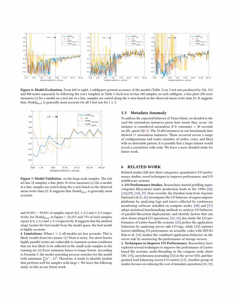
We evaluate Modelbest , Modellocal_best and Modelor iдinal on

4 test sets, plot the results in Figures 6 and 7, and draw 4 major

conclusions below.

1. The identiied features are efective predictors of output

burst performance. Figure 6 shows that, for a model on a test

set with t ≥ 5, 63.28% Ð 96.51% and 76.84% Ð 98.84% of samples

report ∥ϵ ∥ ≤ 0.2 and ≤ 0.3 respectively. Similarly, Figure 7 shows

that, for a model with t ≥ 5, 43.75% Ð 56.25% and 62.5%Ð75% of

samples report ∥ϵ ∥ ≤ 0.2 and ≤ 0.3 respectively. It suggests that

all 3 models are generally accurate across all 4 test sets if a write

operation takes ≥ 5 seconds: the features we choose are efective

to capture output behavior of the target environment.

2. Feature transformation is useful. Figures 6 and 7 also suggest

that Modelbest is generally more accurate than Modelor iдinal for

all 4 test sets: feature transformation is useful to address non-linear

relationships between output performance and its features under

linear regression.

3. The modeling methodology identiies good models. For

t ≥ 5, Modelbest is most accurate for all 4 test sets. Moreover,

for Modelbest on a test set with t ≥ 5 in Figure 6, 83.05% Ð 96.51%

0.12 0.99 2.20 3.48 6.96 11.64 34.72 132.48

samples sorted by t, unit:sec

-1

-0.8

-0.6

-0.4

-0.2

0

0.2

0.4

0.6

0.8

1

Modelbest

t=5

Modellocal_best

Modeloriginal

t=5

0.90 2.62 3.97 5.81 17.04 36.43 59.71 193.25

samples sorted by t, unit:sec

-1

-0.8

-0.6

-0.4

-0.2

0

0.2

0.4

0.6

0.8

1

Modelbest

t=5

Modellocal_best

Modeloriginal

t=5

0.33 1.02 2.65 6.42 14.63 32.63 81.38 381.19

samples sorted by t, unit:sec

-1

-0.8

-0.6

-0.4

-0.2

0

0.2

0.4

0.6

0.8

1

Modelbest

t=5

Modellocal_best

Modeloriginal

t=5

Figure 6: Model Evaluation. From left to right, 3 subigures present accuracy of the models (Table 7) on 3 test sets produced by 256, 512

and 800 nodes separately by following the row1 template in Table 5. Each test set has 280 samples; in each subigure, a line plots 280 error

measures (ϵ) for a model on a test set; in a line, samples are sorted along the x-axis based on the observed mean write time (t ). It suggests

that, Modelbest is generally most accurate for all 3 test sets for t ≥ 5.

0.68 1.18 4.80 31.93 61.21 167.48 344.34

samples sorted by t, unit:sec

-1

-0.8

-0.6

-0.4

-0.2

0

0.2

0.4

0.6

0.8

1

modelbest

t=5

modellocal_best

modeloriginal

t=5

Figure 7: Model Validation on the large-scale samples. The test

set has 18 samples; a line plots 18 error measures (ϵ) for a model;

in a line, samples are sorted along the x-axis based on the observed

mean write time (t ). It suggests that Modelbest is generally most

accurate.

and 89.83% Ð 98.84% of samples report ∥ϵ ∥ ≤ 0.2 and ≤ 0.3 respec-

tively; for Modelbest in Figure 7, 56.25% and 75% of such samples

report ∥ϵ ∥ ≤ 0.2 and ≤ 0.3 respectively. It suggests that the method-

ology locates the best model from the model space; the best model

is highly accurate.

4. Limitations. When t < 5, all models are less accurate. This is

likely results from two issues: (1) Titan is noisy. For short bursts,

highly parallel writes are vulnerable to transient system conditions

that are less likely to be relected in the small-scale samples in the

training set. (2) Error estimator biases to longer bursts. According

to Formula 9, the model searching process searches for the model

with minimum∑(t ′ − t )2. Therefore, it tends to identify models

that perform well for samples with large t . We leave the followup

study on this as our future work.

5.3 Metadata Anomaly

To address the expected behavior of Titan/Atlas2, we decided to dis-

card the anomalous instances given how rarely they occur. An

instance is considered anomalous if it consumes > 30 seconds

on ile_open() (ğ3.1). The 35,404 instances in our benchmark data

showed 17 anomalous instances. These occurred across a range

of conigurations and scales (number of nodes, cores, and iles)

with no detectable pattern. It is possible that a larger dataset would

reveal a correlation with scale. We leave a more detailed study for

future work.

6 RELATED WORK

Related studies fall into three categories: quantitative I/O perfor-

mance studies, novel techniques to improve performance, and I/O

middleware systems.

1. I/O Performance Studies. Researchers started proiling super-

computer ilesystems under production loads in the 1990s [28],

[14],[29], [10], [9]. More recently, the Darshan team from Argonne

National Lab [3, 26] investigates the I/O behavior of supercomputer

platforms by analyzing logs and traces collected by continuous

monitoring software installed on compute nodes. [40] and [37]

adopt statistical benchmarking methods to analyze I/O behavior

of parallel ilesystem deployments, and identify factors that can

slow down striped I/O operations. [22, 25] also study the I/O per-

formance of Lustre-based ile systems: [22] probes the application

behaviors by analyzing server side I/O logs, while [25] explores

factors inhibiting I/O performance on scientiic codes with MPI-IO.

Kim et al. [18] studies the combined application behavior on the

server side by monitoring the performance of storage servers.

2. Techniques to Improve I/O Performance. Researchers have

explored several techniques to improve the performance of Lustre-

based ile systems: multi-threading in the compute node client

OSC [35], asynchronous journaling [32] in the server OSS, and ine-

grained load balancing across I/O routers [13]. Another group of

studies focuses on reducing the cost of metadata operations [23, 33].

Model Name Cost Intercept tmetadata tnode (tt itan*) trouter tsion toss tost (tspider2*) tnoise

Modelbest 44.46 minutes 0.65-0.19 0.005 4.64−7 1.00−9 0.002 0.15 -0.58

log() ()3/4 ()3/2 ()3/2 ()1 log() ()3/2

Modellocal_best 0.18 minute 3.04-0.51 0.0004 1.65−5 1.32−5

log() ()1 ()1 ()3/2

Modelor iдinal 0.0003 minute 1.03-0.001 0.0002 0.0002 −4.13−6 0.003 -0.0004 -2.16

()1 ()1 ()1 ()1 ()1 ()1 ()1

Table 7: Three Trained Models deined in ğ5.2. In this table, features are deined in ğ4.1 and given in Table 3; Modelbest and Modelor iдinalhave the same 7 features with diferent feature transformation functions; Modellocal_best has 4 features. For each model, we report its cost,

intercept and features; for each feature (column 4-10), we report its name, coeicient (a numeric value) and feature transformation function

(Table 4). *: Modellocal_best ’s features.

3. I/O Middleware Systems. I/O middleware systems provide a

high-level I/O API for applications and adapts I/O patterns and con-

igurations automatically to improve I/O performance. ADIOS [8,

20, 24] is a widely used I/Omiddleware system for HPC applications

on supercomputers. Our work is complementary to middleware

systems: for example, they can use I/O system performance pro-

iles and prediction results to guide their coniguration choices and

adapt I/O patterns.

Studies on cloud and data center workloads have investigated

machine learning techniques to predict performance. For exam-

ple, [38] and [11] adopt linear regression and SVD (Singular Value

Decomposition) separately to predict end-to-end application exe-

cution time and drive co-scheduling choices. Compared to their

works, we address an I/O system that provides massively parallel

I/O for individual HPC applications, and apply a systematic model-

ing methodology for the multi-stage write path in a petascale I/O

deployment under production load. To our knowledge our work is

the irst to apply machine learning regression models to analyze

and predict I/O performance for HPC systems and applications.

7 CONCLUSION

Scientiic codes generate periodic parallel output bursts in regular

patterns. We propose a statistical approach to benchmark a pro-

duction petascale I/O system and learn performance models that

can predict output performance seen by applications. We show

that accurate models can be learned based on a few key features of

the deployment and I/O coniguration parameters. Our premise is

that accurate prediction models can guide coniguration choices to

reduce I/O cost, and also provide better information to the global

scheduler, which can use this information to improve resource

utilization.

The major obstacle to building the quantitative I/O analysis on

petascale ilesystems is the high degree of performance variabil-

ity in production deployments. We ind that although the output

performance of petascale ilesystems is highly variable, the mean

performance for suiciently large bursts is predictable.

This paper develops a regression approach to predict output

performance of petascale ilesystems under production load, fo-

cusing on the mean write time. We select and transform features

to capture the properties of the target multi-stage write path and

their impact on I/O performance. We introduce a semi-random sam-

pling method to generate performance datasets to train the models

with low benchmarking cost. A systematic modeling methodology

obtains the best model from a rich model space of features and

transformations. The results suggest that the model is suiciently

accurate to predict performance for suiciently large write bursts

in practice. The key limitation is that small bursts are vulnerable to

transient contention, and so are diicult to predict accurately.

8 ACKNOWLEDGMENTS

We are thankful to the anonymous reviewers and our shepherd

Gabriel Antoniu for their invaluable feedback; to Choong-Seock

Chang and Randy M. Churchill from PPPL for their help on un-

derstanding XGC; to Chris Zimmer and Matt Ezell from OLCF for

their detailed explanations on Titan and Spider 2; to Norbert Pod-

horszki from ORNL and Philip Carns from ANL for their advice

on I/O behavior of HPC codes; to Sayan Mukherjee at Duke for

helpful suggestions on machine learning techniques; to Suzanne

T. Parete-Koon at ORNL for her help on arranging Titan time for

experiments.

This work was supported by the U.S. Department of Energy, un-

der FWP 16-018666, program manager Lucy Nowell. The work used

resources of the Oak Ridge Leadership Computing Facility, located

in the National Center for Computational Sciences at the Oak Ridge

National Laboratory, which is supported by the Oice of Science of

the Department of Energy under Contract DE-AC05-00OR22725.

Sandia National Laboratories is a multi-program laboratory man-

aged and operated by Sandia Corporation, a wholly owned sub-

sidiary of Lockheed Martin Corporation, for the U.S. Department of

Energy’s National Nuclear Security Administration under contract

DE-AC04-94AL85000.

REFERENCES[1] M. Berger and J. Oliger. 1984. Adaptive mesh reinement for hyperbolic partial

diferential equations. Journal of computational Physics 53, 3 (1984), 484ś512.[2] P. Carns, K. Harms, W. Allcock, C. Bacon, S. Lang, R. Latham, and R. Ross. 2011.

Understanding and improving computational science storage access throughcontinuous characterization. ACM Transactions on Storage (TOS) 7, 3 (2011),8ś26.

[3] P. Carns, R. Latham, R. Ross, K. Iskra, S. Lang, and K. Riley. 2009. 24/7 charac-terization of petascale I/O workloads. In Proceedings of 2009 IEEE InternationalConference on Cluster Computing (Cluster’09). IEEE, New Orleans, LA, 1ś10.

[4] L. Chacón. 2004. A non-staggered, conservative, inite-volume scheme for 3Dimplicit extended magnetohydrodynamics in curvilinear geometries. ComputerPhysics Communications 163, 3 (2004), 143 ś 171.

[5] C. S. Chang, S. Klasky, J. Cummings, R. Samtaney, A. Shoshani, L. Sugiyama,D. Keyes, S. Ku, G. Park, S. Parker, and others. 2008. Toward a irst-principlesintegrated simulation of tokamak edge plasmas. Journal of Physics: ConferenceSeries 125, 1 (2008), 012042.

[6] C. S. Chang and S. Ku. 2008. Spontaneous rotation sources in a quiescent tokamakedge plasma. Physics of Plasmas 15, 6 (2008), 062510.

[7] J. H. Chen, A. Choudhary, B. de Supinski, M. DeVries, E. R. Hawkes, S. Klasky,W. Liao, K. Ma, J. Mellor-Crummey, N. Podhorszki, R. Sankaran, S. Shende, andC. Yoo. 2009. Terascale direct numerical simulations of turbulent combustionusing S3D. Computational Science & Discovery 2, 1 (2009), 015001.

[8] A. Choudhary, W. Liao, K. Gao, A. Nisar, R. Ross, R. Thakur, and R. Latham. 2009.Scalable I/O and analytics. Journal of Physics: Conference Series 180, 1 (2009),012048.

[9] P. E. Crandall, R. A. Aydt, A. A. Chien, and D. A. Reed. 1995. Input/Outputcharacteristics of scalable parallel applications. In Proceedings of the ACM/IEEEConference on Supercomputing (SC’95). ACM, San Diego, CA, 59ś89.

[10] R. Cypher, A. Ho, S. Konstantinidou, and P. Messina. 1993. Architectural re-quirements of parallel scientiic applications with explicit communication. InProceedings of the 20th Annual International Symposium on Computer Architecture(ISCA’93). ACM, San Diego, CA, 2ś13.

[11] C. Delimitrou and C. Kozyrakis. 2013. Paragon: QoS-aware scheduling for het-erogeneous datacenters. In Proceedings of the 18th ACM International Conferenceon Architectural Support for Programming Languages and Operating Systems(ASPLOS’13). ATM, Houston, TX, 77ś88.

[12] D. A. Dillow, G. M. Shipman, S. Oral, Z. Zhang, and Y. Kim. 2011. EnhancingI/O throughput via eicient routing and placement for large-scale parallel ilesystems. In Proceedings of the 30th IEEE International Performance Computingand Communications Conference (IPCCC’11). IEEE, Orlando, FL, 21ś29.

[13] M. Ezell, S. Oral, F. Wang, D. Tiwari, D. Maxwell, D. Leverman, and J. Hill. 2014.I/O router placement and ine-grained routing on Titan to support Spider II.In Proceedings of the Cray User Group Conference (CUG’14). cug.org, Lugano,Switzerland, 1ś6.

[14] G. R. Ganger. 1995. Generating representative synthetic workloads: an unsolvedproblem. In Proceedings of the Computer Measurement Group Conference (CMG’95).CMG, Nashville, TN, 1263ś1269.

[15] J. Han, J. Pei, and M. Kamber. 2011. Data mining: concepts and techniques (3 ed.).Morgan Kaufmann, Waltham, MA.

[16] Y. Kim, S. Atchley, G. Vallée, and G. Shipman. 2015. LADS: optimizing datatransfers using layout-aware data scheduling. In Proceedings of the 13th USENIXConference on File and Storage Technologies (FAST’15). USENIX, Santa Clara, CA,67ś80.

[17] Y. Kim and R. Gunasekaran. 2014. Understanding I/O workload characteristics ofa peta-scale storage system. The Journal of Supercomputing 71, 3 (2014), 761ś780.

[18] Y. Kim, R. Gunasekaran, G. M. Shipman, D. A. Dillow, Z. Zhang, and B. W.Settlemyer. 2010. Workload characterization of a leadership class storage cluster.In Proceedings of the 5th Petascale Data Storage Workshop (PDSW’10). ACM, NewOrleans, LA, 1ś5.

[19] S. Klasky, S. Ethier, Z. Lin, K. Martins, D. McCune, and R. Samtaney. 2003. Grid-based parallel data streaming implemented for the Gyrokinetic Toroidal Code.In Proceedings of the ACM/IEEE International Conference for High PerformanceComputing, Networking, Storage and Analysis (SC’03). IEEE, Phoenix, AZ, 24ś36.

[20] S. Kumar, J. Edwards, P.-T. Bremer, A. Knoll, C. Christensen, V. Vishwanath, P.Carns, J. A. Schmidt, and V. Pascucci. 2014. Eicient I/O and storage of adaptive-resolution data. In Proceedings of the ACM/IEEE International Conference for HighPerformance Computing, Networking, Storage and Analysis (SC’14). ACM, NewOrleans, LA, 413ś423.

[21] N. Liu, J. Cope, P. Carns, C. Carothers, R. Ross, G. Grider, A. Crume, and C.Maltzahn. 2012. On the role of burst bufers in leadership-class storage systems.In Proceedings of the 28th IEEE Conference on Massive Data Storage (MSST’12).IEEE, Long Beach, CA, 1ś11.

[22] Y. Liu, R. Gunasekaran, X. Ma, and S. S. Vazhkudai. 2014. Automatic identiicationof application I/O signatures from noisy server-side traces. In Proceedings ofthe 12th USENIX Conference on File and Storage Technologies (FAST’14). USENIX,Santa Clara, CA, 213ś228.

[23] J. Lofstead, F. Zheng, S. Klasky, and K. Schwan. 2009. Adaptable, metadata-richI/O methods for portable high performance I/O. In Proceedings of the 23rd IEEEInternational Parallel & Distributed Processing Symposium (IPDPS’09). IEEE, Rome,Italy, 1ś10.

[24] J. Lofstead, F. Zheng, Q. Liu, S. Klasky, R. Oldield, T. Kordenbrock, K. Schwan,and M. Wolf. 2010. Managing variability in the I/O performance of petascalestorage systems. In Proceedings of the ACM/IEEE International Conference forHigh Performance Computing, Networking, Storage and Analysis (SC’10). ACM,Washington, DC, 1ś12.

[25] J. Logan and P. Dickens. 2008. Towards an understanding of the performance ofMPI-IO in Lustre ile systems. In Proceedings of the IEEE International Conferenceon Cluster Computing (CLUSTER’08). IEEE, Tsukuba, Japan, 330ś335.

[26] H. Luu, M. Winslett, W. Gropp, R. Ross, P. Carns, K. Harms, M. Prabhat, S.Byna, and Y. Yao. 2015. A multiplatform study of I/O behavior on petascalesupercomputers. In Proceedings of the 24th International Symposium on High-Performance Parallel and Distributed Computing (HPDC’15). ACM, Portland, OR,33ś44.

[27] R. Miller, J. Hill, D. A. Dillow, R. Gunasekaran, G. Shipman, and D. Maxwell.2010. Monitoring tools for large scale systems. In Proceedings of Cray User GroupConference (CUG’10). cug.org, Edinburgh, 1ś4.

[28] A. L. Narasimha Reddy and P. Banerjee. 1990. A study of I/O behavior of perfectbenchmarks on a multiprocessor. In Proceedings of the 17th Annual InternationalSymposium on Computer Architecture (ISCA’90). ACM, Seattle, WA, 312ś321.

[29] N. Nieuwejaar, D. Kotz, A. Purakayastha, C. S. Ellis, and M. L. Best. 1996. File-access characteristics of parallel scientiic workloads. IEEE Trans. on Parallel andDistributed Systems 7, 10 (1996), 1075ś1089.

[30] S. Oral, D. A. Dillow, D. Fuller, J. Hill, D. Leverman, S. S. Vazhkudai, F. Wang, Y.Kim, J. Rogers, J. Simmons, and R. Miller. 2013. OLCF’s 1 TB/s, next-generationLustre ile system. In Proceedings of The Cray User Group Conference (CUG’13).cug.org, Napa, California, 1ś4.

[31] S. Oral, J. Simmons, J. Hill, D. Leverman, F. Wang, M. Ezell, R. Miller, D. Fuller, R.Gunasekaran, Y. Kim, S. Gupta, D. Tiwari, S. S. Vazhkudai, J. H. Rogers, D. Dillow,G. M. Shipman, and A. S. Bland. 2014. Best practices and lessons learned fromdeploying and operating large-scale data-centric parallel ile systems. In Proceed-ings of the ACM/IEEE International Conference for High Performance Computing,Networking, Storage and Analysis (SC’14). ACM, New Orleans, LA, 217ś228.

[32] S. Oral, F. Wang, D. Dillow, G. Shipman, R. Miller, and O. Drokin. 2010. Eicientobject storage journaling in a distributed parallel ile system. In Proceedings ofthe 8th USENIX Conference on File and Storage Technologies (FAST’10). USENIX,San Jose, CA, 143ś154.

[33] K. Ren, Q. Zheng, S. Patil, and G. Gibson. 2014. IndexFS: scaling ile system meta-data performance with stateless caching and bulk insertion. In Proceedings of theACM/IEEE International Conference for High Performance Computing, Networking,Storage and Analysis (SC’14). ACM, New Orleans, LA, 237ś248.

[34] scikit learn. 2016. scikit-learn:machine learning in Python. http://scikit-learn.org/. (2016). Accessed: 2016-08-29.

[35] G. Shipman, D. Dillow, D. Fuller, R. Gunasekaran, J. Hill, Y. Kim, S. Oral, D. Reitz, J.Simmons, and F. Wang. 2012. A next-generation parallel ile system environmentfor the OLCF. In Proceedings of the Cray User Group Conference (CUG’12). cug.org,Stuttgart, Germany, 1ś12.

[36] E. Strohmaier, J. Dongarra, H. Simon, and M. Meuer. 2016. Top500 supercomputersites. http://www.top500.org. (2016). Accessed: 2016-08-11.

[37] A. Uselton, M. Howison, N. J. Wright, D. Skinner, N. Keen, J. Shalf, K. L. Kara-vanic, and L. Oliker. 2010. Parallel I/O performance: from events to ensembles.In Proceedings of the 24th IEEE International Parallel & Distributed ProcessingSymposium (IPDPS’10). IEEE, Atlanta, GA, 1ś11.

[38] S. Venkataraman, Z. Yang, M. Franklin, B. Recht, and I. Stoica. 2016. Ernest:eicient performance prediction for large-scale advanced analytics. In Proceedingsof the 13th USENIX Symposium on Networked Systems Design and Implementation(NSDI’16). USENIX, Santa Clara, CA, 363ś378.

[39] F. Wang, S. Oral, G. Shipman, O. Drokin, T. Wang, and I. Huang. 2009. Under-standing Lustre ilesystem internals. Technical Report ORNL TM-2009, 117 (2009),1ś80.

[40] B. Xie, J. Chase, D. Dillow, O. Drokin, S. Klasky, S. Oral, and N. Podhorszki. 2012.Characterizing output bottlenecks in a supercomputer. In Proceedings of theACM/IEEE International Conference for High Performance Computing, Networking,Storage and Analysis (SC’12). IEEE Computer Society Press, Salt Lake City, UT,1ś11.