predicting native pasture growth in the victoria river ... · caz smith who are the current...
TRANSCRIPT

Predicting native pasture growth in the Victoria River
District of the Northern Territory
A thesis submitted by
Michael D. Cobiac B. App. Sc. (Ag.)
to the
School of Agriculture, Food and Wine
Faculty of Sciences
The University of Adelaide, Australia
as fulfilment of the requirements of
Doctor of Philosophy
December 2006

ii
Declaration of Originality
This work contains no material which has been accepted for the award of any other degree
or diploma in any university or other tertiary institution and, to the best of my knowledge
and belief, contains no material previously published or written by another person, except
where due reference has been made in the text.
I give consent to this copy of my thesis, when deposited in the University Library, being
made available in all forms of media, now or hereafter known.
Signed:
Michael Cobiac
Date:

iii
Acknowledgments
The successful completion of this study has involved considerable assistance from many
people throughout the planning, research, analysis, and reporting phases. The efforts of the
following people are gratefully acknowledged.
Funding: The fieldwork and GRASP model calibration reported in this study were funded
by Meat and Livestock Australia’s (MLA’s) North Australia Program. In addition, MLA’s
provision of a Junior Research Fellowship allowed me to concentrate full time on
finalising this thesis. Their contribution has been central to the completion of this work.
My principal supervisor Dr Bill Bellotti (The University of Adelaide) for encouraging me
down the post-graduate path, always being available for advice when needed during the
preparation of this thesis, and his quiet insistence that I produced work of a high standard.
The role of supervisor is crucial to a student’s candidature, and I have been very fortunate
having Bill’s guidance throughout my study.
My co-supervisor Ken Day (Qld Dept. of Natural Resources and Mines) for a great many
things. He provided advice on field data collection, collaborated with me during calibration
of the GRASP model, and reviewed my work many times. Mostly, however, I thank Ken
for his undying faith, patience and friendship throughout the course of this study. This
work would never have been completed without his commitment, and for that I am
indebted.
Dr Greg McKeon (Qld Dept. of Natural Resources and Mines) for his repeated efforts to
educate me about the GRASP model, his endless enthusiasm for the quest to improve
landscape use by the northern Australian pastoral industry, and leading me to think in ways
I never knew were possible. It has been a privilege to work with a scientist of his calibre.
Former NT Dept. of Primary Industry and Fisheries (now DPIFM) staff: Tom Stockwell
for the job; Rodd Dyer for being a great friend and demonstrating work ethic like I’d never
seen before; and Anne Lyon, Bruno Hogan, Linda Cafe and the staff of Victoria River
Research Station (Kidman Springs) for being good mates and for assistance with collection
of data in the field, sometimes under very difficult conditions.

iv
Neil MacDonald, Robyn Cowley, Trudi Oxley, Kieren McCosker, Annemarie Huey and
Caz Smith who are the current generation of bright minds at Katherine Research Station
furthering our understanding of sustainable pastoralism in the semi-arid tropics of the NT.
It is a great motivating factor to know the outcomes of this work will (indeed already do)
play a significant role in ongoing pastoral research.
The NT Cattlemans Association and the producers of the Victoria River District for
allowing me to conduct field research on their properties, for access to confidential
property data, and for their hospitality and open-minded discussions over many years. This
thesis is ultimately for them, the people who manage the landscape.
Shafiq, Ali, Eun-Young, Yasmine, Bagarath, Juan, Vahid and Bandara: the international
postgraduate students at The University of Adelaide’s School of Agriculture, Food and
Wine for befriending me, broadening my mind, and who present their theses in English - to
them a second language. As challenging as things got sometimes, nothing in my study was
as hard as that.
The many other people with whom I interacted during this study and who provided
encouragement when the path forward seemed long, arduous and unclear.
Most importantly, I thank Cath for putting up with my long absences, understanding my
need to see this study through to completion, and supporting me when it was needed most.
Her faith in me carried me through many moments of doubt.

v
Abstract
Pastoralism is the major economic activity in the Victoria River District (VRD), and is
dependent on sustainable pasture use. Analysing grazing practices for sustainability
requires knowledge of annual pasture production, but little quantitative data is available. A
study was undertaken to develop the capacity for predicting native pasture growth in the
VRD using systems modelling. Twenty one field sites were studied for two years using a
standard methodology, and the Grass Production (GRASP) model was calibrated using this
field data. End of growing season total standing dry matter (TSDM) was well predicted
(mean = 2513kg/ha, r2(1:1) = 0.966, RMSE = 132kg/ha, and 98% of predictions within
measurement variance).
Developing generic parameters for common soil and pasture types allowed extrapolation of
the model. Predictive skill declined when using generic parameters (r2(1:1) = -0.265,
RMSE = 807kg/ha and 64% of predictions within measurement variance). However,
observation and prediction means were very similar, indicating that generic parameters are
suitable for broad scale applications, but site-specific parameters are necessary if a high
degree of accuracy is required. Parameters controlling plant water uptake largely determine
pasture growth in low rainfall years, while nitrogen uptake and dilution parameters limit
growth in high rainfall years. Pasture growth is constrained by nitrogen supply in 91% of
seasons in the northern VRD, and in 25% of seasons in the drier south.
Example applications of the model were demonstrated. Current and expected future levels
of pasture utilisation in the district were calculated, showing a current average of 16%,
rising to an expected 20% in the next decade. These levels are within the safe utilisation
rates recommended for the region. Economic analysis shows positive returns ($4.54
million per year) from pasture augmentation with introduced legumes if past problems with
establishment and persistence can be overcome.
Model performance would be improved by accounting for simultaneous wetting of the
entire profile in cracking clay soils, calculating growth of perennial and annual pasture
species separately, and simulating variation in nitrogen uptake and dilution between years.
Incorporation of these processes must be balanced against the increased complexity of the
model and the additional data required for calibration.

vi
Table of Contents
Declaration of Originality ...................................................................................................ii
Acknowledgments .............................................................................................................. iii
Abstract.................................................................................................................................v
Table of Contents ................................................................................................................vi
List of Figures................................................................................................................... viii
List of Tables .....................................................................................................................xiv
List of Plates ................................................................................................................... xviii
1.0 Introduction................................................................................................................1
2.0 Review of literature....................................................................................................5
2.1 A brief description of the Victoria River District ................................................................ 5 2.2 The pastoral industry............................................................................................................ 9 2.3 Current understanding of factors influencing pasture growth............................................ 11 2.4 A modelling approach to assessing pasture growth ........................................................... 20 2.5 Testing the performance of a systems model..................................................................... 28 2.6 The role of systems modelling in grazing land management............................................. 33 2.7 Conclusions........................................................................................................................ 34 2.8 Outline of the study ahead ................................................................................................. 34
3.0 A field study of native pasture growth in the VRD...............................................36
3.1 Introduction........................................................................................................................ 36 3.2 Rationale for obtaining data to calibrate the GRASP pasture growth model..................... 37 3.3 Methods of data collection................................................................................................. 38 3.4 Field results ........................................................................................................................ 50 3.5 Discussion of field study results ...................................................................................... 105 3.6 Conclusions...................................................................................................................... 117
4.0 Analysis of field measurements using a systems modelling approach ..............119
4.1 Introduction...................................................................................................................... 119 4.2 An overview of the GRASP pasture growth model ......................................................... 121 4.3 Method for deriving model parameters and calibrating GRASP ..................................... 127 4.4 Results of calibration: Final model parameters................................................................ 133 4.5 Comparing model outputs with field data........................................................................ 143 4.6 Discussion of the calibration procedure and modelling results........................................ 156 4.7 Conclusions...................................................................................................................... 169
5.0 Testing the performance of GRASP for application to the wider landscape ...170
5.1 Introduction...................................................................................................................... 170

vii
5.2 Generic parameters suitable for extrapolation across the landscape ................................171 5.3 Testing model performance using independent data ........................................................177 5.4 Discussion of independent validation of GRASP.............................................................186 5.5 Conclusions ......................................................................................................................189
6.0 Determining parameters most influential on predictions of long-term pasture
growth ...............................................................................................................................190
6.1 Introduction ......................................................................................................................190 6.2 Modelling year-to-year variability in pasture growth across a climate gradient ..............191 6.3 Sensitivity of model predictions to changes in value of influential parameters ...............200 6.4 The effect of trees on predictions of pasture growth ........................................................205 6.5 Discussion.........................................................................................................................208 6.6 Conclusions ......................................................................................................................213
7.0 Implications for analysing grazing practices in the VRD: examples of model
application ........................................................................................................................214
7.1 Introduction ......................................................................................................................214 7.2 Pasture utilisation in the VRD ..........................................................................................215 7.3 Potential benefits of alleviating the nitrogen limitation to pasture growth.......................228 7.4 Discussion.........................................................................................................................241 7.5 Conclusions ......................................................................................................................248
8.0 Integrating discussion and final conclusions of study ........................................249
8.1 Introduction ......................................................................................................................249 8.2 The capacity to predict pasture growth in the VRD .........................................................249 8.3 Limitations of the systems modelling approach used in this study ..................................252 8.4 Recommendations for future work ...................................................................................256 8.5 Final conclusion................................................................................................................257
Appendices........................................................................................................................258
References.........................................................................................................................311

viii
List of Figures
Chapter 1
Figure 1.1 The location of the Victoria River District of the Northern Territory. ............................................ 2
Figure 1.2 Illustration of the structure of this thesis. ........................................................................................ 4
Chapter 2
Figure 2.1 Seasonal rainfall (July to June, mm) at Victoria River Downs Station for the period 1900/01 to
2003/04. The horizontal dashed line represents the median value (639mm) (Source: DataDrill 2005). ........... 6
Figure 2.2 Land tenure in the Victoria River District in 2004 (data sourced from NT Dept of Lands). ........... 8
Figure 2.3 Total cattle population and annual turnoff (number of animals sold) for the Victoria River
District 1883 – 2004 (S. Murti pers.comm., based on Australian Bureau of Statistics and NT Office of
Resource Development data). Dashed lines represent interpolation across periods where no data is available.
Early data has been left as isolated points as no basis for interpolation is available. ...................................... 10
Figure 2.4 Annual trends in LI, TI, MI and GI values at Katherine, NT for: a) tropical grasses, and b) tropical
legumes; c) the relationship between mean daily temperature (0F) and fractional dry matter production in
three groups of pastures (Fitzpatrick and Nix 1970)........................................................................................ 23
Figure 2.5 a) Thermal response curves of tropical grasses and legumes including the solid line used in the
study of McCown (1981a); b) moisture index function of McCown et al. (1974). ......................................... 25
Figure 2.6 Structure of the water balance model and pasture sub-model in GRASP (Littleboy and McKeon
1997)................................................................................................................................................................ 27
Figure 2.7 Examples of GRASP model output for individual seasons, and over 15 years from Johnston
(1996). ............................................................................................................................................................. 28
Figure 2.8 Examples of two approaches to model testing from Mitchell and Sheehy (1997). ....................... 32
Chapter 3
Figure 3.1 The structure of Chapter 3. ............................................................................................................ 37
Figure 3.2 The five main locations of the study sites within the Victoria River District (shaded area). Dashed
lines represent approximate average annual rainfall isohyets (Source: adapted from BoM data). .................. 40
Figure 3.3 Design and layout of study site showing cells (dashed line squares) and an example pattern of
quadrat placement (solid line squares) for each pasture measurement (H1 to H8). Quadrat location for each
pasture measurement was randomised for each site. ....................................................................................... 42
Figure 3.4 Time-series of management and data collection from each site over the study period.................. 51
Figure 3.5 Maximum and minimum daily temperatures (0C) at Mt Sanford (17012’S, 130036’E) over the
study period (upper graph) compared to the 7-day moving averages of 47-year values (1957/58 – 2003/04);

ix
and measured daily rainfall averaged across Sites 1-6 (lower graph). Temperature data derived from
DataDrill (2005)............................................................................................................................................... 54
Figure 3.6 Total monthly measured rainfall at Mt Sanford averaged across Sites 1-6, and 47-year median
values (1957/58 – 2003/04) derived from DataDrill (2005). ........................................................................... 54
Figure 3.7 Maximum and minimum daily temperatures (0C) at Kidman Springs (16006’S, 131000’E) over the
study period (upper graph) compared to the 7-day moving averages of 47-year values (1957/58 – 2003/04);
and measured daily rainfall averaged across Sites 7-12 for 1993/94, Sites 7-14 for 1994/95 and Sites 13-14
for 1995/96 (lower graph). Temperature data derived from DataDrill (2005)................................................. 55
Figure 3.8 Total monthly measured rainfall at Kidman Springs averaged across Sites 7-12 for 1993/94, Sites
7-14 for 1994/95 and Sites 13-14 for 1995/96, and 47-year median values (1957/58 – 2003/04) derived from
DataDrill (2005)............................................................................................................................................... 55
Figure 3.9 Maximum and minimum daily temperatures (0C) at Victoria River Downs (16024’S, 131006’E)
over the study period (upper graph) compared to the 7-day moving averages of 47-year values (1957/58 –
2003/04); and measured daily rainfall at the station homestead (lower graph). Temperature data derived from
DataDrill (2005)............................................................................................................................................... 56
Figure 3.10 Total monthly measured rainfall at Victoria River Downs homestead, and 47-year median values
(1957/58 – 2003/04) derived from DataDrill (2005). ...................................................................................... 56
Figure 3.11 Maximum and minimum daily temperatures (0C) at Rosewood (16030’S, 129000’E) over the
study period (upper graph) compared to the 7-day moving averages of 47-year values (1957/58 – 2003/04);
and measured daily rainfall at the station homestead (lower graph). Temperature data derived from DataDrill
(2005)............................................................................................................................................................... 57
Figure 3.12 Total monthly measured rainfall at Rosewood homestead, and 47-year median values (1957/58 –
2003/04) derived from DataDrill (2005).......................................................................................................... 57
Figure 3.13 Maximum and minimum daily temperatures (0C) at Auvergne (15024’S, 130000’E) over the
study period (upper graph) compared to the 7-day moving averages of 47-year values (1957/58 – 2003/04);
and measured daily rainfall at the station homestead (lower graph). Temperature data derived from DataDrill
(2005)............................................................................................................................................................... 58
Figure 3.14 Total monthly measured rainfall at Auvergne homestead, and 47-year median values (1957/58 –
2003/04) derived from DataDrill (2005).......................................................................................................... 58
Figure 3.15 Field-measured soil water contents of sites located on red earths overlying basalt. .................... 63
Figure 3.16 Field-measured soil water contents of sites located on red earth overlying limestone. ............... 65
Figure 3.17 Field-measured soil water contents of sites located on cracking clays overlying basalt.............. 67
Figure 3.18 Field-measured soil water contents of sites located on cracking clays of alluvial origin. ........... 71
Figure 3.19 The observed phases of plant growth during the study period for: a) the annual short grass
Brachyachne convergens; b) the annual mid-height grass Iseilema vaginiflorum; c) the perennial tussock
grass Astrebla pectinata; and d) the perennial tuft grass Chrysopogon fallax................................................. 80
Figure 3.20 Pasture composition of three sites dominated by barley Mitchell grass. Error bars indicate the
standard error of the site mean for total standing dry matter at each sampling time (harvest). ....................... 82

x
Figure 3.21 Pasture nitrogen contents (dashed lines) and nitrogen uptake (vertical bars) of three sites
dominated by barley Mitchell grass................................................................................................................. 83
Figure 3.22 Plots of total standing dry matter (TSDM) against: a) total plant cover; and b) plant height for
sites dominated by barley Mitchell grass......................................................................................................... 84
Figure 3.23 Pasture composition of three sites dominated by ribbon grass. Error bars indicate the standard
error of the site mean for total standing dry matter at each sampling time (harvest)....................................... 87
Figure 3.24 Pasture nitrogen contents (dashed lines) and nitrogen uptake (vertical bars) of three sites
dominated by ribbon grass............................................................................................................................... 88
Figure 3.25 Plots of total standing dry matter (TSDM) against: a) total plant cover; and b) plant height for
sites dominated by ribbon grass....................................................................................................................... 90
Figure 3.26 Pasture composition of three sites dominated by other perennial grass species. Error bars
indicate the standard error of the site mean for total standing dry matter at each sampling time (harvest). .... 92
Figure 3.27 Pasture nitrogen contents (dashed lines) and nitrogen uptake (vertical bars) of three sites
dominated by other perennial grass species..................................................................................................... 93
Figure 3.28 Plots of total standing dry matter (TSDM) against: a) total plant cover; and b) plant height for
sites dominated by other perennial grass species............................................................................................. 95
Figure 3.29 Pasture composition of sites dominated by annual short grass species. Error bars indicate the
standard error of the site mean for total standing dry matter at each sampling time (harvest). ....................... 97
Figure 3.30 Pasture nitrogen contents (dashed lines) and nitrogen uptake (vertical bars) of sites dominated by
annual short grass species. ............................................................................................................................... 98
Figure 3.31 Plots of total standing dry matter (TSDM) against: a) total plant cover; and b) plant height for
sites dominated by annual short grass species. ................................................................................................ 99
Figure 3.32 Pasture composition of sites dominated by forb species. Error bars indicate the standard error of
the site mean for total standing dry matter at each sampling time (harvest).................................................. 102
Figure 3.33 Pasture nitrogen contents (dashed lines) and nitrogen uptake (vertical bars) of sites dominated by
forb species. ................................................................................................................................................... 103
Figure 3.34 Plots of total standing dry matter (TSDM) against: a) total plant cover; and b) plant height for
sites dominated by forb species. .................................................................................................................... 104
Figure 3.35 Relationships between perennial grass basal area (PGBA) and end of growing season standing
dry matter (SDM) of a) perennial grasses; b) annual grasses and forbs; and c) total pasture........................ 115
Chapter 4
Figure 4.1 The structure of Chapter 4. .......................................................................................................... 120
Figure 4.2 The four phases of systems analysis (bolded text in box) and an indication of where the
components of this study fit within this framework (after Grant et al. 1997)................................................ 120
Figure 4.3 Relationship between accumulated pasture transpiration and nitrogen uptake (from Littleboy and
McKeon 1997). The user-defined coefficients for stored plant N reserves, N uptake per 100mm of

xi
transpiration, and maximum N available for uptake shown in this figure are realistic for the semi-arid tropics,
but are examples only. ................................................................................................................................... 124
Figure 4.4 Flow of dry matter through the biomass pools (bolded) in the pasture system (modified from
Littleboy and McKeon 1997). Processes that transfer dry matter from one biomass pool to another are
presented in italics. ........................................................................................................................................ 125
Figure 4.5 Typical daily biomass accumulation curve for native pasture in the Victoria River District,
including approximate times of field measurements and the parameters in GRASP that are calibrated from
data collected at these times........................................................................................................................... 133
Figure 4.6 Examples of time-series plots of prediction curves (lines) with observed values (points, including
95% confidence limits in the TSDM plots). Data presented are from sites of different soil type and pasture
species composition: Site 4 (forbs on basalt clay); Site 8 (ribbon grass on alluvial clay); Site 1 (annual short
grasses on basalt red earth); Site 14 (other perennial grasses on limestone red earth); Site 5 (barley Mitchell
grass on basalt clay); Site 12 (other perennial grasses on limestone red earth); Site 3 (barley Mitchell grass on
basalt clay); and Site 15 (forbs on alluvial clay)............................................................................................ 148
Figure 4.7 Observed vs. predicted data for all sites. Model predictions are the results of using individual site
parameter sets. Variables presented are total standing dry matter (TSDM), nitrogen uptake (N uptake), plant
available water content in the 0-50cm layer of the soil (PAWC), and green plant cover. Associated statistics
are presented in Table 4.7. ............................................................................................................................. 151
Figure 4.8 Deviation of predictions (points) from observed values (line of zero deviation) of total standing
dry matter for all sites and years. Predictions are generated by GRASP using the individual parameter sets
presented in Table 4.1 to Table 4.6. Dashed lines indicate the envelope of acceptable precision, equal to the
average magnitude of measurement variance (±35% of observation values). ............................................... 155
Figure 4.9 Deviation of prediction values (points) from their corresponding observations of TSDM (x on line
of zero deviation and including 95% confidence limits) for Site 4 and Site 8. .............................................. 155
Figure 4.10 Deviation of predictions (points) from observed values of total standing dry matter (x on line of
zero deviation and including 95% confidence limits) for all observations less than 500kg/ha...................... 164
Chapter 5
Figure 5.1 The structure of Chapter 5. .......................................................................................................... 171
Figure 5.2 Illustration of the procedure for assembling data for the independent validation of GRASP, using
the annual short grasses group as an example. S01Y1 refers to Site 1, Year 1; S01Y2 refers to Site 1, Year 2;
and so on. ....................................................................................................................................................... 180
Figure 5.3 Observed vs. predicted TSDM for independent model validation using four approaches to
developing generic parameter sets. ................................................................................................................ 183
Figure 5.4 Deviation of predictions (points) from observed values (line of zero deviation) of total standing
dry matter (TSDM) during independent validation. Predictions are generated by GRASP using four
approaches to developing generic group parameter sets (Table 5.2). Dashed lines indicate the envelope of

xii
acceptable precision, equal to the average magnitude of measurement variance (±35% of observation values).
....................................................................................................................................................................... 184
Chapter 6
Figure 6.1 The structure of Chapter 6. .......................................................................................................... 191
Figure 6.2 Time-series of simulated seasonal pasture growth (SSPG, July to June) over a 45-year period
(1959/60 to 2003/04) using the Regional VRD parameter set at three locations in the VRD. ....................... 198
Figure 6.3 Probability distribution of simulated seasonal pasture growth (SSPG, July to June) over a 45-year
period (1959/60 to 2003/04) using the Regional VRD parameter set at three locations in the VRD. The
horizontal dashed line represents the median (50th percentile) value............................................................. 198
Figure 6.4 Probability distributions of simulated seasonal pasture growth (SSPG, July to June) over a 45-
year period (1959/60 to 2003/04) using a) five Species group parameter sets; and b) three Soil group
parameter sets at Victoria River Downs. Horizontal dashed lines represents median (50th percentile) values.
....................................................................................................................................................................... 198
Figure 6.4...................................................................................................................................................... 199
Figure 6.5 a) Time-series of seasonal rainfall (July to June); and b) relationship between seasonal rainfall
and simulated seasonal pasture growth (SSPG) over a 45-year period (1959/60 to 2003/04) using Regional
VRD parameters at three locations in the VRD. The plotted regression is for seasons when SSPG was less
than the upper limit of 3345kg/ha.................................................................................................................. 199
Figure 6.6 a) Time-series of cumulative seasonal transpiration (July to June); and b) relationship between
seasonal transpiration and simulated seasonal pasture growth (SSPG) over a 45-year period (1959/60 to
2003/04) using Regional VRD parameters at three locations in the VRD. The plotted regression is for seasons
when SSPG was less than the upper limit of 3345kg/ha................................................................................ 199
Figure 6.7 a) Time-series of nitrogen uptake (July to June); and b) relationship between N uptake and
simulated seasonal pasture growth (SSPG) over a 45-year period (1959/60 to 2003/04) using Regional VRD
parameters at three locations in the VRD. The plotted regression is for seasons when N uptake was less than
the upper limit of 24kg/ha/year...................................................................................................................... 199
Figure 6.8 Sensitivity of simulated seasonal pasture growth results (SSPG) using a standard parameter set at
Victoria River Downs to changes in values of transpiration-use-efficiency, green yield at 50% green cover,
and soil water index at which growth stops. The horizontal dashed lines represent the median (50th percentile)
value. ............................................................................................................................................................. 203
Figure 6.9 Sensitivity of simulated seasonal pasture growth (SSPG) using a standard parameter set at
Victoria River Downs to changes in values of maximum N uptake, N content at which growth stops, and N
uptake per 100mm of transpiration. The horizontal dashed lines represent the median (50th percentile) value.
....................................................................................................................................................................... 204
Figure 6.10 Time-series of simulated seasonal pasture growth (SSPG, July to June) in the absence and the
presence of trees over 45 years (1959/60 to 2003/04) at a) Auvergne (mean annual rainfall = 900mm); and b)

xiii
Inverway (mean annual rainfall = 577mm). Tree basal area (TBA) was set at 6.0m2/ha at Auvergne and
2.0m2/ha at Inverway. .................................................................................................................................... 207
Figure 6.11 Probability distribution of simulated seasonal pasture growth (SSPG) in the absence and the
presence of trees over 45 years (1959/60 to 2003/04) at two locations in the VRD. ..................................... 207
Figure 6.12 Presentation yield of tallgrass pasture at the end of growing season in lightly grazed native
pasture woodlands at Manbulloo, near Katherine NT (McIvor et al. 1994) and GRASP predictions of
seasonal pasture growth (July to June) using Regional VRD parameters and tree basal area of 7.0m2/ha..... 207
Chapter 7
Figure 7.1 The structure of Chapter 7. .......................................................................................................... 214
Figure 7.2 Relationship between intake at long-term stocking rate and median simulated seasonal pasture
growth (SSPG) across 10 properties in the VRD using stocking rate data provided in the 1997 survey (Smith
1998) and pasture growth predicted using the Soil x Species approach to developing generic parameters. The
dashed line represents a similar relationship from three regions in Queensland (Hall et al. 1998). .............. 223
Figure 7.3 Effect of climate variability on annual pasture utilisation over a 45 year period (1959/60 to
2003/2004) when a constant stocking rate is maintained (district average = 9.2AE/km2, Table 7.4)............ 227
Figure 7.4 Effect of climate variability on annual stocking rate over a 45 year period (1959/60 to 2003/2004)
when a constant utilisation rate is maintained (district average = 16.3%, Table 7.4). ................................... 227
Figure 7.5 a) Time-series; and b) probability distribution of simulated seasonal pasture growth (SSPG) in the
absence of trees over 45-year period (1959/60 to 2003/04) using Regional VRD parameters at Auvergne
when maximum nitrogen supply (MaxN) is limited (24kg/ha, the observed district average) and theoretically
unlimited (96kg/ha)........................................................................................................................................ 233
Figure 7.6 Relationship between simulated seasonal pasture growth (SSPG, July to June) and a) seasonal
transpiration (July to June); and b) total nitrogen uptake in the absence of trees over 45 years (1959/60 to
2003/04) at Auvergne when maximum nitrogen supply (MaxN) is limited (24kg/ha, the observed district
average) and theoretically unlimited (96kg/ha). ............................................................................................ 234
Appendices
Figure 9.1 Pasture composition results not presented in Chapter 3. Error bars indicate the standard error of
the site mean for total standing dry matter at each sampling time (harvest). (Figure continued overleaf) .... 280
Figure 9.2 Pasture nitrogen contents (dashed lines) and nitrogen uptake (vertical bars) of sites not presented
in Chapter 3. (Figure continued overleaf) ...................................................................................................... 282

xiv
List of Tables
Chapter 2
Table 2.1 Climate data at Victoria River Downs Station for the period 1900/01 to 2003/04 (source: DataDrill
2005).................................................................................................................................................................. 6
Table 2.2 Summary of existing pasture production data for the VRD. ........................................................... 19
Chapter 3
Table 3.1 Matrix of land systems by parent material and soil type (adapted from Stewart et al. 1970). ........ 39
Table 3.2 General description of the 21 study sites at 5 locations in the Victoria River District (VRD)........ 44
Table 3.3 Measured seasonal rainfall (July - June) over the study period, the 47-year (1957/58 – 2003/04)
median value, and rainfall percentiles. Median data calculated from DataDrill (2005). ................................. 53
Table 3.4 Monthly values for radiation, evaporation and vapour pressure deficit at Victoria River Downs
during the study period (source: DataDrill 2005). ........................................................................................... 60
Table 3.5 Soil description for sites located on red earths overlying basalt. .................................................... 62
Table 3.6 Physical properties of soils at sites located on red earths overlying basalt. .................................... 62
Table 3.7 Soil description for sites located on red earths overlying limestone. .............................................. 64
Table 3.8 Physical properties of soils at sites located on red earths overlying limestone. .............................. 64
Table 3.9 Soil description for sites located on cracking clays overlying basalt. ............................................. 66
Table 3.10 Physical properties of soils at sites located on cracking clays overlying basalt. ........................... 67
Table 3.11 Soil description for sites located on cracking clays of alluvial origin........................................... 69
Table 3.12 Physical properties of soils at sites located on cracking clays of alluvial origin........................... 70
Table 3.13 Example to demonstrate extrapolating soil moisture values to missing data points. .................... 73
Table 3.14 Estimated dates of initiation of pasture growth for each study location, based on criteria of
receiving both 50mm of rain within 14 days and 75mm within 28 days of the initiation date. ....................... 77
Table 3.15 Main pasture and tree species present during the study period for sites dominated by barley
Mitchell grass (Astrebla pectinata).................................................................................................................. 81
Table 3.16 Results for N and P status of pasture at sites dominated by barley Mitchell grass. ...................... 84
Table 3.17 Some important pasture variables at sites dominated by barley Mitchell grass. ........................... 84
Table 3.18 Main pasture and tree species present during the study period for sites dominated by ribbon grass
(Chrysopogon fallax). ...................................................................................................................................... 86
Table 3.19 Results for N and P status of pasture at sites dominated by ribbon grass. .................................... 89
Table 3.20 Some important pasture variables at sites dominated by ribbon grass. ......................................... 89

xv
Table 3.21 Main pasture and tree species present during the study period for sites dominated by other
perennial grass species..................................................................................................................................... 91
Table 3.22 Results for N and P status of pasture at sites dominated by other perennial grass species............ 94
Table 3.23 Some important pasture variables at sites dominated by other perennial grass species. ............... 94
Table 3.24 Main pasture and tree species present during the study period for sites dominated by annual short
grass species..................................................................................................................................................... 96
Table 3.25 Results for N and P status of pasture at sites dominated by annual short grass species. ............... 99
Table 3.26 Some important pasture variables at sites dominated by annual short grass species..................... 99
Table 3.27 Main pasture and tree species present during the study period for sites dominated by forb species.
....................................................................................................................................................................... 101
Table 3.28 Results for N and P status of pasture at sites dominated by forb species. ................................... 104
Table 3.29 Some important pasture variables at sites dominated by forb species......................................... 104
Table 3.30 Variability in rainfall at the five study locations in the VRD. Rainfall data from DataDrill (2005).
....................................................................................................................................................................... 106
Table 3.31 Summary of results for important soil variables. ........................................................................ 109
Table 3.32 Summary of soil chemistry results for each of the major soil types in this study. ...................... 110
Table 3.33 Summary of field results for important pasture variables. .......................................................... 112
Table 3.34 Variance in field measurements of total standing dry matter (TSDM) for 21 sites over two years.
Values represent 95% confidence limits expressed as a proportion of the harvest mean. ............................. 113
Chapter 4
Table 4.1 Site-by-year calibrated GRASP soil parameters. (Table continued overleaf) ............................... 135
Table 4.2 Site-by-year calibrated GRASP sward structure parameters. (Table continued below)................ 138
Table 4.3 Site-by-year calibrated GRASP plant growth parameters. (Table continued below).................... 139
Table 4.4 Site-by-year calibrated GRASP nitrogen parameters. (Table continued below)........................... 140
Table 4.5 Tree parameters for Site 19. .......................................................................................................... 141
Table 4.6 Site-by-year calibrated GRASP detachment parameters. (Table continued below)...................... 142
Table 4.7 Results of statistical comparison of predictions and observed values for all sites, using individual
site parameter sets. Data presented is total standing dry matter (TSDM), plant available water content of the
0-50cm layer of the soil (PAWC), nitrogen uptake (N uptake), and green plant cover (Cover).................... 153
Table 4.8 Summary of the number of predictions of TSDM that fell outside the envelopes of acceptable
precision......................................................................................................................................................... 156
Table 4.9 Summary of parameter values derived during calibration of GRASP to the study sites. .............. 158
Table 4.10 Summary of model calibration results for total standing dry matter. .......................................... 162

xvi
Chapter 5
Table 5.1 Matrix of study sites (numbers in table) as they relate to soil and species groups for development
of generic parameter sets. .............................................................................................................................. 172
Table 5.2 Generic parameter values for Soil, Species, and Regional VRD groups. (Table continued overleaf)
....................................................................................................................................................................... 175
Table 5.3 Source of parameters used to calculate partial estimates for independent model validation. This
table is based upon the matrix presented in Table 5.1. .................................................................................. 181
Table 5.4 Results of comparing model predictions with observed values of TSDM for independent validation
using four approaches to developing generic parameter sets......................................................................... 185
Table 5.5 Summary of predictions of TSDM that fell outside the envelopes of acceptable precision (95%
confidence limits of the corresponding observation) using four approaches to developing generic parameter
sets. ................................................................................................................................................................ 185
Table 5.6 Summary of results of independent validation of GRASP (including comparative results from
calibration in Chapter 4) for end of wet season total standing dry matter. .................................................... 188
Chapter 6
Table 6.1 Summary of year-to-year variation in predictions of pasture growth over 45 years at three locations
in the VRD..................................................................................................................................................... 209
Chapter 7
Table 7.1 Some estimates of long-term safe levels of pasture utilisation across northern Australia............. 216
Table 7.2 Stocking rate and burning frequency for each land system in the 1997 survey; and estimations of
tree basal area, closest associated generic pasture and soil parameters, and estimated soil depth for each land
system. ........................................................................................................................................................... 221
Table 7.3 Median simulated seasonal pasture growth (SSPG) calculated using the Site x Species approach to
developing generic parameters; and long term utilisation rates for specific land systems on 10 properties in
the VRD, using stocking rate data provided in the 1997 survey (Smith 1998).............................................. 224
Table 7.4 Current and expected future stocking rates (SR) and levels of pasture utilisation (Util) on 22
properties in the VRD using property carrying capacity and grazing area data from the 2004 survey (Oxley
2006). Pasture growth used to determine utilisation calculated from the Regional VRD parameter set at
Victoria River Downs. ................................................................................................................................... 226
Table 7.5 Comparison of simulated key nitrogen and pasture variables under nitrogen-limited and unlimited
conditions, and in the presence and absence of trees at Auvergne over a 45 year period (1959/60 to 2003/04).
Values across each row are not necessarily from the same season................................................................ 234
Table 7.6 Year-to-year costs of augmenting native pasture with legumes in the northern Ord-Victoria Area
(adapted from Oxley and Walker (2003). Pastures require renovation and re-establishment after 10 years. All
values are $/ha. .............................................................................................................................................. 238

xvii
Table 7.7 Projected benefit of augmenting native pastures with legumes in the northern Ord-Victoria Area.
....................................................................................................................................................................... 239
Table 7.8 Sensitivity of benefit-cost analysis to changes in input values. Base values are those used in
calculation of costs (Table 7.6) and projected benefits (Table 7.7). Percentage change for net regional benefit
is relative to the base value of $4.54million. ................................................................................................. 240
Table 7.9 Predicted percentiles of: utilisation at four constant stocking rates; and stocking rates at four
constant levels of utilisation. Calculations based on pasture growth predictions over a 45 year period
(1959/60 to 2003/2004) at Victoria River Downs using the Regional VRD parameter set. ........................... 244
Chapter 8
Table 8.1 Summary of the current suitability of GRASP for application to analysis of grazing practices in the
VRD when using parameters developed in this study. .................................................................................. 251
Appendices
Table 9.1 Study sites classified using: 1 Perry (1970); 2 Stewart et al. (1970); and 3 DIPE (unpublished). .. 268
Table 9.2 Study sites classified according to: 1 Northcote (1979); 2 Northcote et al. (1975); 3 Stace et al.
(1968); 4 Isbell (1996); 5 McDonald et al. (1990). ......................................................................................... 269
Table 9.3 Study sites classified according to Wilson et al. (1990)................................................................ 270
Table 9.4 Study sites classified according to Tothill and Gillies (1992)....................................................... 271
Table 9.5 Laboratory analysis results of soil samples from sites located on red earths overlying basalt...... 272
Table 9.6 Laboratory analysis results of soil samples from sites located on red earths overlying limestone.
....................................................................................................................................................................... 273
Table 9.7 Laboratory analysis results of soil samples from sites located on cracking clays overlying basalt.
....................................................................................................................................................................... 273
Table 9.8 Laboratory analysis results of soil samples from sites located on cracking clays of alluvial origin.
....................................................................................................................................................................... 274
Table 9.9 Amount of soil nutrients present in surface layers of study sites. (Table continued overleaf) ...... 275
Table 9.10 Plant species nomenclature for all individual species presented in this study............................. 278
Table 9.11 Complete list of plant species present at Site 1, July 1995.......................................................... 279
Table 9.12 Descriptive statistics for total standing dry matter data collected at each harvest for all sites. Eight
1m2 quadrats were cut at each harvest. All units are kg/ha. (Table continued overleaf)................................ 284
Table 9.13 Observed and predicted total standing dry matter (TSDM) values from GRASP model calibration.
(Table continued overleaf)............................................................................................................................. 290
Table 9.14 Summary of results from parameter sensitivity analysis. Data presented is end of growing season
pasture TSDM. All units are kg/ha. ............................................................................................................... 297

xviii
List of Plates
Appendices
Plate 1 Northern Victoria River District landscape showing escarpment country, woodland plains and
alluvial flats. .................................................................................................................................................. 258
Plate 2 Central Victoria River District landscape showing cattle grazing Chrysopogon fallax and Iseilema
spp. pasture on cracking clay soil. ................................................................................................................. 258
Plate 3 Southern Victoria River District landscape showing open grassy plains with scattered trees and
occasional rocky basalt outcrops. .................................................................................................................. 259
Plate 4 Land showing evidence of past heavy grazing: bare and scalded ground, dead trees, and annual
pasture species. .............................................................................................................................................. 259
Plate 5 Fencing a study site to exclude cattle from grazing. ......................................................................... 260
Plate 6 Burning to remove carryover material at commencement of the study period (Site 16)................... 260
Plate 7 Marking out sampling cells at site establishment (Site 2). ................................................................ 260
Plate 8 a) Bulk density sampling in soil profile pit; and b) hand-augering soil moisture cores during field
measurements. ............................................................................................................................................... 261
Plate 9 a) Measuring perennial grass basal area using a 5-point frame; and b) pasture sampling during field
measurements. ............................................................................................................................................... 261
Plate 10 Red earth overlying basalt (Site 19). ............................................................................................... 262
Plate 11 Red earth overlying limestone (Site 11).......................................................................................... 262
Plate 12 Cracking clay overlying basalt (Site 4). .......................................................................................... 263
Plate 13 Alluvial cracking clay (Site 7). ....................................................................................................... 263
Plate 14 Barley Mitchell grass pasture (Site 18). .......................................................................................... 264
Plate 15 Overhead view of 1m2 quadrat in a) barley Mitchell grass pasture (Site 18); and b) ribbon grass
pasture (Site 8)............................................................................................................................................... 264
Plate 16 Ribbon grass pasture (Site 8). ......................................................................................................... 264
Plate 17 White grass pasture (Site 14). ......................................................................................................... 265
Plate 18 Overhead view of 1m2 quadrat in a) white grass pasture (Site 14); and b) annual short grass pasture
(Site 1). .......................................................................................................................................................... 265
Plate 19 Annual short grass pasture (Site 1). ................................................................................................ 265
Plate 20 Forb pasture (Site 4)........................................................................................................................ 266
Plate 21 a) Overhead view of 1m2 quadrat in a forb pasture (Site 4); and b) an example of the abundant,
diverse forbs present at Site 15 on 2 May 1995............................................................................................. 266
Plate 22 Inundated conditions at Site 15 on 9 March 1995........................................................................... 266

xix
Plate 23 Annual short grass pasture early in the wet season with no burning at site establishment (Site 13, 12
Jan 1995)........................................................................................................................................................ 267
Plate 24 Overhead view of 1m2 quadrats in an annual short grass pasture (Site 13) during early wet season a)
with no burning at site establishment; and b) after burning to remove carryover material............................ 267
Plate 25 Annual short grass pasture early in the wet season after site burnt to remove carryover material (Site
13, 9 Jan 1996). Fire most likely destroyed much of the seed bank, resulting in poor germination. ............. 267

Chapter 1 Introduction
1
1.0 Introduction
The production of beef cattle from native pastures (pastoralism) is the main economic use
of tropical woodlands across northern Australia today, as it has been for more than a
century (MacLeod et al. 2004). In the Victoria River District of the Northern Territory
(Figure 1.1), attempts to develop land for crop production and replace native pastures with
exotic species have been limited by overriding climatic constraints and low fertility soils
(Bauer 1985). Consequently, pastoralism is the dominant land use in the Victoria River
District (VRD) and this is unlikely to change in the foreseeable future.
For much of its history the pastoral industry in the VRD had little control over herds, and
cattle populations fluctuated depending upon prevailing seasonal conditions. Occasional
periods of high grazing pressure occurred, particularly on favoured pasture types and close
to stock drinking water. Some periods of high grazing pressure resulted in land degradation
(Condon 1986; Tothill and Gillies 1992). Land degradation reduces the productivity and
profitability of pastoral enterprises (MacLeod et al. 2004). Improvements to property
infrastructure over the past few decades have increased control over the timing, intensity
and duration of grazing. Control of grazing allows for development of improved grazing
practices that minimise the risk of future degradation episodes.
A crucial component of long-term sustainable use of native pastures is balancing cattle
demand for feed with the amount of pasture available (MLA 2004b). Climate has long
been recognised as a major determinant of pasture production. Therefore, achieving the
balance between forage demand and pasture production requires knowledge of the
relationships between climate and pasture growth (McKeon et al. 1990). Despite the long
history of grazing in the region, little quantitative data on long-term pasture production is
available and this is a severe limitation to analysis of grazing practices. A means of
predicting pasture growth using climate data would benefit the development, evaluation
and improvement of management practices for grazed native pastures in the VRD.
Aim of this study
This study aims to develop the capacity for predicting native pasture growth in the Victoria
River District of the Northern Territory and demonstrate application of that capacity to
analysis of grazing practices.

Chapter 1 Introduction
2
Figure 1.1 The location of the Victoria River District of the Northern Territory.
Research approach
To achieve this aim, Chapter 2 first describes the features of the VRD and its pastoral
industry. The current knowledge the factors affecting pasture production are then
reviewed, revealing a need to quantify the long-term productivity of native pastures in the
region. The development of systems modelling as a means of quantifying pasture
productivity for application to grazing management is discussed and the GRASP pasture
growth model (Littleboy and McKeon 1997) is briefly described.
Chapter 3 documents a field study that collected the necessary data to establish
relationships between climate, soil water supply and pasture growth for commonly grazed
native pasture communities throughout the region. This data is used in Chapter 4 to adapt
(calibrate) GRASP for simulating the pasture system at the study locations. When a model
is calibrated from field data, the process involves closely fitting model output to the field
observations. Chapter 4 briefly describes the calibration process and then concentrates on
evaluating the degree of fit between model predictions and measured data. The input
parameter values derived for each location form the basis for extending the use of the
model beyond the boundaries of this study.
At this stage of the thesis, results of model calibration are specific to the individual site
during the period of field measurements. On their own, they are of limited value for
application to analysis of grazing practices. Before GRASP can be applied for grazing
Katherine
Victoria River Downs Station
Northern TerritoryInverway Station
Auvergne Station
Darwin
Alice Springs
Victoria River
District

Chapter 1 Introduction
3
management purposes, the capability of the model to replicate events (i.e. pasture growth)
at times and places for which field data has not been collected is tested. Two steps are
necessary to test the model in this manner: 1) individual site parameters are summarised to
form generic parameters representing land types of interest; and 2) simulation results when
using generic parameters are compared with independent measured data to evaluate the
ability of GRASP to simulate growth of native pastures across the region. The process of
summarising individual site parameters to form generic parameter sets and testing model
with independent data is described in Chapter 5.
McKeon et al. (1990) points out that some individual model parameters have greater
influence on predictions of pasture growth than others. Using generic values for these
parameters may compromise accurate simulation of the pasture system in some instances.
Identifying the parameters which have most influence on model behaviour in the VRD will
provide future model users with guidance when selecting appropriate parameter values and
interpreting the results of their simulation studies. Chapter 6 documents the process and
outcomes of identifying these influential parameters and their effect on predictions of
pasture growth.
The purpose of developing a capacity to predict native pasture growth is to facilitate the
development and analysis of sustainable grazing practices. GRASP has been used as a tool
for assisting grazing management since the early 1990’s (e.g. McKeon et al. 1994;
Johnston et al. 1996a; Day et al. 1997b; Hall et al. 2001) and has many applications. This
thesis will demonstrate two applications of a well-tested model to grazing land
management in the VRD: 1) calculating current and expected future levels of pasture
utilisation (the proportion of annual pasture growth consumed by grazing cattle) in the
VRD; and 2) the effect of improving the nitrogen supply (a known constraint to pasture
growth) in the northern high rainfall zone of the district. These applications are presented
in Chapter 7. An integrating discussion of the findings of this study leads to the final study
conclusions in Chapter 8.
The approach to structuring this thesis is based upon Evans and Gruba (2002), although
numerous departures from their recommendations occur. An illustrative representation of
the structure is presented in Figure 1.2.

Chapter 1 Introduction
4
Figure 1.2 Illustration of the structure of this thesis.
Background and reason for study Chapter 2
Calibration of GRASP to each individual site
Chapter 4
Assessing the fit between model results and field data
Field study methods
Climate results Soil results Pasture results
Chapter 3
Identifying major influences on pasture growth
Chapter 6
Final discussion and conclusions of study
Chapter 8
Generic parameters for testing model with independent data
VRD as a region Pasture types Soil types Chapter 5
Evaluating the capability of GRASP for extrapolation to the wider landscape of the VRD
Applications of model to management of grazing land
Current and future levels of pasture utilisation
Chapter 7 Alleviating the nitrogen limit to
pasture growth

Chapter 2 Review of Literature
5
2.0 Review of literature
2.1 A brief description of the Victoria River District
Physical descriptions of the region are given in CSIRO (1970) and Muchow (1985), and a
relevant summary of northern Australia is given by Shaw and Norman (1970). Kraatz
(2000) provides a concise overview of the natural environment of the VRD and similar
information is accessible online at the Tropical Savannas Cooperative Research Centre
website (TSCRC 2006). These descriptions are summarised below to provide a basic
outline of the region. Photographic examples of landscape in the northern, central and
southern VRD are shown in Plate 1, Plate 2, and Plate 3 respectively (Appendix 1).
Location
The Victoria River District (VRD) is a region of about 126 000km2 lying between the
latitudes 150S and 190S and longitudes 1290E and 1320E in the northwest of the Northern
Territory (NT) of Australia. The boundaries of the district are the Joseph Bonaparte Gulf
coastline and the Fitzmaurice and Flora Rivers to the north, the Sturt Plateau to the east,
the Tanami Desert to the south, and the Western Australian border and Kimberley region
to the west. Figure 1.1 and Figure 3.2 show the location of the VRD within the NT.
Climate
Climate in the VRD has been described by Slatyer (1960), Slatyer (1970) and Williams et
al. (1985) and more generally by Tothill et al. (1985), Partridge (1994) and Colls and
Whittaker (2001). The region can be classified as having a semi-arid tropical (monsoonal)
climate with hot, wet and humid summers during which 95% of annual rainfall occurs; and
sunny, warm and dry winters that are virtually rainless. Short transitional periods merge
these two distinct seasons. A climate summary for Victoria River Downs Station in the
centre of the district is shown in Figure 2.1 and Table 2.1. The data highlights the generally
high temperatures of the region, strong seasonal and year-to-year variability of rainfall,
seasonal variation in humidity, and high evaporative demand throughout the year.

Chapter 2 Review of Literature ------------------------------------------------------------------------------------------------------------------------------------------
NOTE: This figure is included on page 6 in the print copy of the thesis held in the University of Adelaide Library.
Figure 2.1 Seasonal rainfall (July to June, mm) at Victoria River Downs Station for the period 1900/01 to 2003/04. The horizontal dashed line represents the median value (639mm) (Source: DataDrill 2005).
Table 2.1 Climate data at Victoria River Downs Station for the period 1900/01 to 2003/04 (source: DataDrill 2005).
Topo
The
on A
altitu
(Pat
____
NOTE: This table is included on page 6 in the print copy of the thesisheld in the University of Adelaide Library.
graphy
major topographic feature of the region is the Victoria River Plateau. It is formed
delaidean sediments and is a large dissected plateau rarely exceeding 350m in
de. It is a collection of structural plateaux and benches, mesas and buttes
erson 1970). This
_____________________________________________________________ 6

Chapter 2 Review of Literature
7
plateau forms the catchment area of the Victoria River, the major watercourse from which
the region takes its name. Much of the area consists of rocks and their resistant nature is
visible across the landscape (Williams et al. 1985).
Geology
Many geologic periods are represented in the VRD. Traves et al. (1970) and Paterson
(1970) give summaries of the geology and geomorphology of the district, including maps.
Isbell (1983) and Johnson (2004) describe the geology of northern Australia in more
general terms, and Kraatz (2000) provides a brief history of geologic activity in the region.
To summarise, the oldest rocks are volcanics, sandstones, and siltstones in the north-
eastern part of the district formed during the Archaean-Lower Proterozoic period (3500 to
1000 million years ago (Mya)). The youngest soils are the Quaternary (<1.8 Mya) alluvia
found on floodplains associated with the coast and major watercourses and drainage
systems of the districts north. Adelaidean (550+ Mya) sediments (sandstone, siltstone,
dolomite, and shale) make up a large proportion of the district’s centre. Lower Cambrian
(545 to 490 Mya) volcanics are the other major geologic group present in the region,
occurring in the western, southern and eastern parts. The desert lands of the very south are
generally Tertiary (65 to 1.8 Mya) laterite.
Soils
Steep tablelands and hills with rock outcrops dominate much of the district and these lands
generally have shallow, immature skeletal soils, with deeper soils restricted to the gentle
slopes and plains (Kraatz 2000). On erosional and alluvial plains there are distinct
relationships between soils and climate, drainage, and parent materials. Stewart (1970b)
outlines these relationships for the major soil groups. Generally speaking, better-drained
sites have medium textured red and yellow earths in higher rainfall areas, and coarse sandy
desert soils in the south. Gentle slopes and poorly drained sites usually have cracking clay
soils. Floodplain alluvia almost invariably consist of cracking clay soils. The most striking
feature of soils in this region is the universal presence of very low levels of nitrogen and
phosphorus (Perry 1960; Isbell 1983; Williams et al. 1985).
Vegetation
In their report on the vegetation of the NT, Wilson et al. (1990) give a summary of
vegetation in the semi-arid zone, within which the VRD lies. They state that the most

Chapter 2 Review of Literature
8
widespread communities in this zone are woodlands and open woodlands. Throughout the
VRD the overstorey component is dominated by the Eucalyptus and Corymbia genera on
most soils, except the clays where Lysiphyllum, Terminalia or Melaleuca occur. The
ground layer is dominated by grasses, particularly long-lived perennials like Sehima,
Heteropogon, Themeda and Sorghum on medium textured soils, Plectrachne on drier soils
and Dichanthium, Chrysopogon and Astrebla on the clays. Other broad descriptions of
vegetation of the region are given by Andrew et al. (1985), Mott et al. (1985) and Kraatz
(2000). More detailed information on individual species can be found in Petheram and Kok
(1983), Vallance et al. (1993), Wheaton (1994) and Moore (2005).
Land Use
About 65% (83 000km2) of the VRD is currently pastoral lease land, and some aboriginal
freehold land is also used for pastoralism. Individual private leaseholders own many of the
30 stations in the district and Aboriginal interests and Australian or international
companies have the rest (Oxley 2006). The remaining land is not used for commercial
production. Figure 2.2 shows proportions of each land tenure type in the district in 2004.
The economic importance of cattle production in the region is described in Section 2.2.
The focus of this study is the grazing lands of the district and although the outcomes of this
work will have some application to non-grazing lands, they are not considered further.
Figure 2.2 Land tenure in the Victoria River District in 2004 (data sourced from NT Dept of Lands).
Pastoral lease65%
Aboriginal freehold14%
National parks11%
Other (mainly defence)
10%

Chapter 2 Review of Literature
9
2.2 The pastoral industry
2.2.1 History
Pastoralism (beef cattle production from native pastures) has been the dominant land use in
the district as it has been since European settlement in the late 1800’s (Perry 1970; Winter
et al. 1985; Kraatz 2000). Traditionally, properties covered huge tracts of land and inputs
from management were very low. Few fences meant cattle movements were largely
uncontrolled and large herds tended to congregate around the natural watering points
(rivers, waterholes and springs). Considerable feral horse and donkey populations were
also present (TSCRC 2006).
Implementation of the Brucellosis and Tuberculosis Eradication Campaign (BTEC) during
the 1970’s lead to substantial changes in the industry. Fences were constructed, bores
drilled to draw cattle away from natural waters, and aerial mustering introduced to improve
the control over stock numbers and movements needed to comply with the campaign’s
testing requirements. Condon (1986) states: “the (BTEC) program has changed the
concept of the cattle industry from a hunting operation of semi-wild cattle to one in which
increasing attention will be paid to the management of the land and animal resource”.
Cattle producer surveys document characteristics of the pastoral industry at this time (Hill
1976; Robertson 1980; Robertson 1982), and a northern Australian context is provided by
O'Rourke et al. (1992).
Today cattle stations in the district are still very large, averaging 3275km2 (327 500ha) of
which 2227km2 (222 700ha) are grazed. Paddocks typically exceed 100km2 (10 000ha).
Herds average 21 500 head per property, giving a district population of over 500 000 head
(Oxley 2006). Annual turnoff (number of animals sold per year) from the VRD over the
past 20 years has averaged about 90 000 head (Figure 2.3), a contribution of about 25%
(over $50m) to the $200m NT beef cattle industry (DPIF and ORD 2001; S. Murti
pers.comm.). Live export of growing cattle is the primary turnoff market (Bortolussi et al.
2005a), with Indonesia and the Philippines the main destinations. Domestic abattoirs and
feedlots take the balance of marketed animals.

Chapter 2 Review of Literature
10
Figure 2.3 Total cattle population and annual turnoff (number of animals sold) for the Victoria River
District 1883 – 2004 (S. Murti pers.comm., based on Australian Bureau of Statistics and NT Office of
Resource Development data). Dashed lines represent interpolation across periods where no data is available.
Early data has been left as isolated points as no basis for interpolation is available.
2.2.2 Grazing management
The low level of grazing management practiced for much of the pastoral industry’s history
is evident by the conspicuous lack of reference to it in the producer surveys of the 1970’s
(Hill 1976; Robertson 1980). Due to improved livestock control and marketing
opportunities, grazing management in the region today is much more sophisticated.
Current knowledge of sustainable grazing management in the VRD has recently been
synthesized into an education package known as Grazing Land Management (GLM) (MLA
2004a). The main elements of GLM are outlined below.
Sustainable management of native pastures for grazing aims to achieve two desirable
outcomes: 1) optimising animal production; and 2) maintaining healthy and productive
land. These outcomes are achieved by attention to three basic principles of grazing land
management:
• improving land condition (conversion of rainfall into useful pastures);
• improving the evenness of pasture use (consumption of pasture by cattle); and
• improving diet quality (converting pasture into beef).
These three principles are directly affected by pasture utilisation; the balance between
pasture supply and the feed requirements of grazing animals. Consequently, sustainable
0
100
200
300
400
500
600
1880 1900 1920 1940 1960 1980 2000
Num
ber o
f Cat
tle (x
1000
) Total cattle populationAnnual turnoff

Chapter 2 Review of Literature
11
grazing management in the VRD relies heavily on knowledge of the productivity of the
native pasture communities used for grazing.
2.3 Current understanding of factors influencing pasture growth
Above-ground grass growth at the individual plant level is a function of energy (radiation
and temperature), water (soil moisture), plant–available nutrients (soil fertility), and gas
(atmospheric CO2) (Fitzpatrick and Nix 1970). At the landscape level, total pasture
biomass production is also a result of species composition, plant density, competition for
water and nutrients with other vegetation groups (e.g. shrubs, trees and exotic weeds),
impacts of fire and grazing defoliation (native and introduced), and pests and diseases.
Some of these factors are of little relevance to this study and, therefore, the following
review is restricted to the most influential factors driving plant growth in the VRD.
Literature relevant to this study uses several expressions relating to the amount of pasture
present in the field. ‘Yield’, ‘biomass’, and ‘total standing dry matter’ refer to the actual
amount of pasture present at any point in time and are often used interchangeably. ‘Pasture
growth’ is used to refer to the amount of pasture dry matter that has accumulated since the
beginning of the growing season in the absence of grazing and excluding any carryover
material from previous seasons. ‘Pasture productivity’ and ‘pasture production’ refer to
total pasture amount present at the end of the growing season in the absence of grazing.
These terms will be applied throughout this thesis in a manner that most clearly expresses
the intended meaning.
2.3.1 The influence of climate
Climate patterns for the northern part of the Northern Territory have been analysed by
several authors (Slatyer 1960; Slatyer 1970; Taylor and Tulloch 1985), each noting the
high level of rainfall variability. The importance of climate as a factor influencing pasture
growth has been well researched and documented. Many attempts have been made to
quantify the relationships between climate variables and pasture growth for tropical
Australia, mostly in a modelling framework. Such frameworks use a soil water balance
approach, combined with defined response functions to other variables (Slatyer 1960;
Fitzpatrick and Nix 1970; McAlpine 1970; McCown et al. 1974; McCown 1981a; McKeon
et al. 1982a; Rickert and McKeon 1982; Littleboy and McKeon 1997). These approaches

Chapter 2 Review of Literature
12
are reviewed in Section 2.4. The following paragraphs summarise the influence of climate
variables on pasture growth in the study area.
Rainfall
Where grass production is highly seasonal, as in the semi-arid tropics of the VRD, grass
production is directly related to rainfall. The amount, distribution, and variability of
rainfall are major factors determining the time of initiation of growth and the period for
which growth will be sustained. Slatyer (1960) states that in relation to plant growth,
climatic factors other than rainfall are of secondary importance at Katherine. In the VRD
rainfall patterns are highly variable with frequent dry spells of varying duration within the
wet season, and this places a limitation on the period during which there is sufficient soil
moisture available for plant growth (Slatyer 1970). Much of the precipitation occurs in
high intensity storms and part of this rainfall becomes surface runoff or infiltrates beyond
the root zone of pasture plants (Williams et al. 1985). Johnson and Tothill (1985) point out
that while annual rainfall totals provide a useful frame of reference, seasonality of the
rainfall pattern, effective rainfall during the growing season, and the duration and effect of
the dry season are of greater importance. Mott et al. (1985) state that the major climatic
constraint to grass production is soil water and hence the highly seasonal nature of rainfall
in the VRD is reflected by the correspondingly seasonal plant growth patterns.
Temperature
Different groups of plants have fundamentally different responses to temperature
(Fitzpatrick and Nix 1970; Sweeney and Hopkinson 1975). The normal extremes of
temperature and when they occur in the annual cycle are most important to pasture growth.
Tropical grasses have high temperature optimums and, while northern Australia
experiences relatively high ambient temperatures, some authors suggest they may not be
sufficient for maximum growth rates. For example, Doley and Trivett (1974) report an
optimum temperature for photosynthesis of 400C for a native perennial grass. However
Christie (1975b) found reduced growth rate of two tropical grasses at this temperature and
report temperature optimums of closer to 300C. Tropical legumes have lower thermal
optimums (Whiteman 1968; Sweeney and Hopkinson 1975) and are likely to grow
unrestricted by temperature in this region, although Fitzpatrick and Nix (1970) suggest that
the high temperatures during the growing season may in fact surpass optimums and
sometimes reduce the growth rate of tropical legumes. Ivory and Whiteman (1978) report

Chapter 2 Review of Literature
13
that growth of subtropical grasses ceases at day temperatures of 12.50C and night
temperatures of 100C. These conditions are rare in the Victoria River District and never
occur during the growing season. Thus, temperature is not a factor in the cessation of
growth in the environment of the VRD.
Slatyer (1960) reports short periods of very high temperatures occurring on occasions
during the wet season and these may have a direct effect on plant development. This is
particularly true when they are associated with periods of low humidity, and occur during
critical periods of plant development such as flowering time.
The occurrence of frost is rare, with the northern parts of the VRD virtually frost free and
southern parts having occasional light frosts in some years, particularly in topographically
suited localities (Slatyer 1970). However, frosts never occur during the period of plant
growth, and are therefore not considered any further in this study.
Radiation and day length
The influence of solar radiation (sunlight) on plant growth depends on the species under
consideration. Photosynthetic rate is a result of interaction between plant structure and
physiological properties, and the physical properties of the incident light (Fitzpatrick and
Nix 1970; Ludlow 1985). Fitzpatrick and Nix (1970) suggest that light is rarely a limiting
factor to plant growth in northern Australia, except for some minor effect during high
rainfall periods when cloud cover reduces incident light. Plant response to photoperiod is
also species-specific. Fitzpatrick and Nix (1970) suggest that some perennial grass species
in the monsoonal tropics are short-day plants; that is, their flowering is initiated by
reducing day-length. For all species, day length during the natural growing season always
exceeds 12 hours and plants are passing through their seed setting and maturing phases at a
time of decreasing day length (Slatyer 1960).
Fitzpatrick and Nix (1970) show the average daily radiation received in the VRD varies
only slightly throughout the year and is always high relative to most of Australia. Values
range from 550cal/cm2/day (23MJ/m2/day) during January, down to 425cal/cm2/day
(17.8MJ/m2/day) in July. Sunshine hours reach a peak in August (300hrs/month). Values
decrease from September to November as cloud cover increases, reach their minimum in
February while monsoon cloud is present, and then steadily increase again until August.

Chapter 2 Review of Literature
14
Day length varies little throughout the year from 11.2 hours per day in June to 13.0 hours
per day in December (Williams et al. 1985). Neither Fitzpatrick and Nix (1970) nor
McCown (1981a) consider solar radiation as a limiting factor in plant growth in the
Australian tropics.
In summary, the amount and distribution of rainfall is the most influential climate variable
on pasture growth in the VRD. Temperature has occasional effects for short periods and
sunlight is nearly always non-limiting.
2.3.2 Limitations to pasture production other than climate
Climate is not the only determinant of pasture production. In their natural state, most
northern Australian soils have low levels of many nutrients important for plant growth
(Williams and Andrew 1970; Schmidt and Lamble 2002). Mott et al. (1985) suggest that
nutrients, either alone or in combination with soil water supply, are important in
determining plant production in semi-arid rangelands. Species composition of the pasture
sward and the presence of other vegetation classes (e.g. trees) also impacts upon pasture
production. These are discussed below.
Nutrients
Mott et al. (1985) state that in some soil/climate systems (e.g. the monsoonal tropics of the
northern VRD), water will always be secondary to nutrients as the major determinant of
seasonal pasture production. In other climates and soils, nutrients and water will interact so
that in some seasons nutrients will be the main controlling factor, whereas in other seasons
it will be water and temperature. Schmidt and Lamble (2002) report a strong link existing
between soil nutrient availability and pasture productivity for northern Australian
savannas, and McIvor et al. (1994) and Cook and Andrew (1991) also support the view
that nutrients are the main limiter of plant growth in the tallgrass systems of the Northern
Territory. Christie (1981) suggests that on some land types in semi-arid Queensland
nitrogen is the major limiting nutrient for biomass production, while on others it is
phosphorus.

Chapter 2 Review of Literature
15
Nitrogen
Nitrogen (N) is quantitatively the most important nutrient that pasture plants take up from
the soil, however N levels are low in most semi-arid areas of Australia (Williams and
Raupach 1983; Schmidt and Lamble 2002). Early agricultural research at Katherine on red
clay soils revealed that nitrogen and phosphorus (P) were the primary limiting nutrients for
plant growth and no others had been identified at that time (Norman 1962). Results in
Norman (1962) demonstrate a marked interaction between N and P in pasture growth
responses. Cook and Andrew (1991) report nitrogen limitations to native pasture growth in
the monsoonal tropics near Darwin, while Friedel et al. (1980) found positive pasture
growth responses by native pasture species to additional N supply under field conditions in
central Australia, but not all species responded equally. Christie (1981) concluded that
nitrogen is the major limiting nutrient for biomass production for the Mitchell grassland
systems in Queensland (and, by inference, those in the NT including the southern VRD).
Herbaceous legumes are a common component of native pastures in the VRD. Similarly, a
number of woody leguminous tree and shrub species occupy some land types. No data is
available on the contribution of these species to soil nitrogen status, although it is
reasonable to assume the major contribution is from decomposition of roots and leaf litter
(Mott et al. 1985; Abbadie et al. 1992). Lawrie (1981) reports nitrogen fixation of less than
1kg/ha in native legumes on a number of soil types in temperate Victoria.
Wetselaar and Hutton (1963) recorded nitrogen contents in rainfall equivalent to adding
around 1.5kg/ha to the soil in a typical wet season, with much of this occurring early in the
season. However, they point out that the origin of this nitrogen is likely to be terrestrial -
from dust, smoke, and volatilisation of nitrogen from the soil surface. They conclude that
such an addition of N is not true accession but rather a cycling of previously lost nutrients.
Phosphorus
Phosphorus is widely deficient in soils across Australia, and present only at low levels in
the ancient, heavily leached soils of tropical Australia (Isbell 1983). McIvor (1984) states
that the ability of a species to grow in low P soils is related to its capacity to absorb P at
low levels and/or a low internal requirement of P for optimum growth. A significant
consequence of phosphorus deficiency in semi-arid grasses is reduced root growth
(Christie 1975a). Experimental work suggested that the native grasses Chrysopogon fallax

Chapter 2 Review of Literature
16
and Heteropogon contortus (both widespread in the VRD) had low requirements for
phosphorus, as did other native grasses in the study (McIvor 1984). Norman (1962) found
mixed responses of native grasses to varying levels of P supply, but general trends were
that additional P supply resulted in increased pasture growth. Christie and Moorby (1975)
report similar findings. Friedel et al. (1980) found that P is potentially even more deficient
in degraded soils than healthy soils in central Australia.
Trees
Johnson and Tothill (1985) define savanna vegetation (native pasture lands) as “a
continuous graminoid stratum more or less interrupted by trees or shrubs”, referring to the
almost universal presence of trees across the landscape of northern Australia. Other authors
also refer to the widespread presence of trees on the savanna lands of northern Australia
(Perry 1970; Mott et al. 1985; Burrows et al. 1990; McKeon et al. 1990; Jackson and Ash
1998) and overseas (Walker et al. 1981). Where pasture and tree root distributions overlap,
they likely compete for water and nutrients (Schmidt and Lamble 2002).
Scanlan (2002) reviewed tree-grass dynamics in Queensland and concluded that pasture
production response to tree density depends upon tree species, rainfall, soil type, climatic
history, fire, and grazing, and will change over time. The relationship between pasture
production and increasing tree density can vary from linear decrease, to exponential
decrease to initial stimulation followed by a decrease.
No published work is available on the competitive relationships between trees and pasture
in the VRD. Eyles et al. (1984) and Winter et al. (1989b) report increased grass production
in the first years following killing of trees in tropical tall-grass pastures near Katherine, but
the effect declined after several years. More recent work at Katherine also found an
increase in pasture production following removal of trees (Cafe et al. 1999). A similar
trend has been observed at Kidman Springs in the central VRD (L.M. Cafe pers.comm.)
and in other semi-arid environments (e.g. south-west Queensland, Beale 1973). Day et al.
(2003) reports considerable competition between trees and pasture for soil nitrogen in the
semi-arid region of Zimbabwe. In the Katherine Region competition between trees and
grasses is greater for nutrients than for soil water (Winter et al. 1989b).

Chapter 2 Review of Literature
17
Species composition
Species composition is primarily determined by climate, soil type and grazing history.
Pasture species composition has been identified by McIvor et al. (1995a) as being of
significance to seasonal biomass production. While they reviewed previous studies on this
topic and the variable trends in pasture production reported in them, their own research on
the monsoonal tall-grasses near Katherine showed that as perennial grass content declined
and annual grasses and forbs increased, total pasture production decreased. This decrease
was associated with an increase in the nitrogen and phosphorus uptake by pasture (Ash and
McIvor 1995), and improved animal liveweight gain (Ash et al. 1995). The increased risk
of further undesirable changes caused by grazing annual species dominated pastures more
than offsets any improvement in animal nutrition.
To summarise, rainfall patterns and soil type influence soil water supply. Soil water and
nutrient availability are the major influences on seasonal pasture production, and species
composition is also an important factor. Scholes (1993) provides this useful synopsis of
pasture growth in the semi-arid tropics: “it is a convenient simplification to consider that
water controls growth duration, while nutrients and temperature control growth rate”.
2.3.3 Previous studies of pasture production in the VRD
The earliest assessment of pasture production in the VRD was in terms of estimated cattle
carrying capacity (number of grazing animals per unit area) for a particular land type.
Early estimations of carrying capacity for pasture lands in the region are reported by Perry
(1960) and Perry (1970).
Some formal assessments of the production of native pasture communities were carried out
in the 1950’s and 1960’s at Katherine Research Station, just outside the VRD. While much
research during this period centred on finding productive introduced species, growth rate
and nutritional studies were made on several native pasture communities (Norman and
Wetselaar 1960; Smith 1960; Norman 1962; Norman 1963a; Norman 1969). These native
pasture studies were restricted to deep soils with agricultural potential close to the
township of Katherine. Potential for beef cattle production from these pastures have also
been experimentally recorded (Norman 1960; Norman 1965; Norman 1967).

Chapter 2 Review of Literature
18
The land units of Kidman Springs in the centre of the district (Figure 3.2) are described by
Forster and Laity (1972). They identify a number of discreet land units and give an
ambiguous grazing value for each unit in words (no grazing, little, rough, productive
grazing etc.) and did not attempt to quantify this with pasture production or recommended
stocking rates. Foran et al. (1985) give data on pasture species composition and standing
biomass under grazed and ungrazed conditions on two pasture communities at Kidman
Springs. Foran et al. (1985) also explore the effect of pasture condition on pasture
production and species composition for a common land type (calcareous red earth), noting
the predominance of arid short grasses on the heavily utilised areas of this land type. Bastin
and Andison (1990) and Bastin et al. (2003) provide an update on those studies, both
noting that prevailing seasonal conditions and grazing history influenced changes in
species composition and hence overall pasture productivity. These results and others from
the studies discussed in the following paragraphs are summarised in Table 2.2.
A description of lands in the western VRD is given by Robinson (1971) and Aldrick et al.
(1978) and, while they make comment on the impact of grazing on species composition,
they make no attempt to estimate pasture production or livestock carrying capacities.
Tothill and Gillies (1992) describe the land types across northern Australia (including the
VRD) using local pasture units (LPU’s). They classify land into one of three pasture
conditions within each LPU. Their classification system, while not clearly defined,
indicates pasture condition, or the health of the pasture communities, is very high in most
of the VRD. However some landscapes, particularly watercourse frontage country, short
grass pastures on red earths, and perennial grasses on cracking clays have experienced
some periods of heavy utilisation in the past and are in a state of ‘modified pristine’ or
slightly deteriorating condition.
Pasture condition was investigated by McIvor et al. (1995a) and Ash and McIvor (1995)
on tropical tall-grass pasture communities in the north-east of the region. These studies
highlighted the importance of both soil and vegetation factors in determining pasture
productivity. Ash et al. (1995) take this further and detail the animal production associated
with differences in pasture condition, highlighting the fact that often animal production can
be enhanced by species composition change from perennial to annual based pasture
swards. Annual species based pastures are, however, at greater risk of fluctuating yields.

Chapter 2 Review of Literature
19
Animal production from such pastures in the long term is therefore less favourable than
from pastures with high perennial grass content.
Since 1993, a grazing trial aimed at determining the relationship between stocking rate and
pasture productivity has been conducted at Mt Sanford in the southern part of the region.
Detailed measurements of species composition and standing pasture yield have been
recorded for the main pasture types present. Results include standing dry matter of various
pasture components under grazing (perennials and annuals, palatable and unpalatable
species, plant cover and bare ground), and pasture utilisation and animal liveweight gains
at different stocking rates (MacDonald et al. 1997; R.N. MacDonald, unpublished data.).
Table 2.2 Summary of existing pasture production data for the VRD.
Location Soil type Pasture species
Grazing intensity
TSDM
(kg/ha)
Years Reference
Katherine Tippera red
earth
Themeda,
Chrysopogon,
Sorghum
Ungrazed 1050 to 1550 1957/58 to
1967/68
Norman 1969
Kidman Springs
Cracking clay Chrysopogon,
Dichanthium,
Iseilema
Ungrazed 800 to 2100 Foran et al. 1985
Calcareous
red earth
Brachyachne,
Sporobolus,
Aristida
Ungrazed 150 to 1991 1973/74 to
1978/79
Calcareous
red earth
Enneapogon Ungrazed 600 to 1590 1973/74 to
1978/79
Calcareous Heteropogon Ungrazed 900 1989 Bastin et al. 2003
red earth 1500 to 2000 1994
1250 1999
1700 to 3000 2002
Manbulloo Red earth Chrysopogon,
Sorghum,
Sehima
Low 1490 to 2240 1981/82 to
1988/89
McIvor et al. 1994
Mt Sanford Cracking clay Astrebla Low 2410 1993/94 to
1998/99
R.N. MacDonald
unpublished data
Various Red earth Brachyachne,
Enneapogon
Low 900 1997/98 to
1998/99
Dyer et al. 2001a
Cracking clay Astrebla Low 1539
Various Sorghum Low 1250
Various Chrysopogon,
Dichanthium
Low 2319

Chapter 2 Review of Literature
20
In summary, some isolated measures of native pasture production have been made in and
around the VRD (Table 2.2), but these measures provide little value for estimating
production at other times and locations. Knowledge of the annual variation in pasture
production due to the influences of climate, soil characteristics, species composition and
plant density does not exist for most of the region. Determining the relationships between
such factors is a complex task, and too large and time-consuming to consider by field
experimentation alone. Another approach is required.
2.4 A modelling approach to assessing pasture growth
One approach to understanding the inter-relationships between factors that govern pasture
productivity, and the range of likely productivity from different land types, is to use
systems modelling. Mathematical modelling of the plant growth system is a well-
developed field and models can calculate plant growth as a product of many influential
factors. A systems modelling approach is currently the only option for providing objective
estimates of pasture productivity where no measurements have been taken. In the
following section previous relevant attempts to model pasture growth are discussed.
McCown et al. (1974) and Grant et al. (1997) give concise explanations of why models of
pasture growth may be used in preference to field studies in order to quantify the long-term
productivity of pasture communities. McCown et al. (1974) state that in the Australian
tropics, short-term trials are insufficient to obtain a quantitative estimate of the likely year-
to-year variation in pasture yield. Furthermore, longer-term trials have serious drawbacks
including difficulty in maintaining original botanical composition and fertility, and
limitation of the scope of research by committing finite research resources to these long-
term trials. McKeon et al. (1990) agree, stating that the development and testing of whole
farm systems is expensive in terms of time and resources if traditional methods of
experimentation are used. Modelling is seen as a practical method of evaluating many
options over longer time periods and for a greater range of environments than can be
achieved with field experimentation (Grant et al. 1997). This view is supported by Alcock
(2006) who states “grazing systems models … are essential tools for analysing the impact
of climate-driven production variability”.

Chapter 2 Review of Literature
21
2.4.1 Development of systems modelling of pasture growth
The approach of using climatic records to estimate plant growth by means of a soil water
balance has been used for many years. Slatyer (1960) details a method for estimating crop
growing season characteristics at Katherine using rainfall, soil water storage capacity and
evapotranspiration. McAlpine (1970) also uses a water balance approach on a weekly time-
step to provide probabilistic estimates of pasture production in central Australia. Johnston
(1996) explains the basis for modelling plant growth: the soil water balance describes
changes in soil moisture in terms of the difference between the input of rainfall and the
output of soil evaporation, plant transpiration, runoff and drainage. Plant growth is
assumed to be proportional to transpiration.
In 1970, Fitzpatrick and Nix introduced the concept of the Growth Index as a simple
empirical model of pasture production for Australian grasslands. They argued that the three
most important climatic variables influencing pasture growth were precipitation, incident
radiation, and temperature. The index of Fitzpatrick and Nix (1970) is described as:
GI = LI * TI * MI (Equation 1)
where: GI is Growth Index
LI is Light (radiation) Index
TI is Temperature Index, and
MI is Moisture Index
All indices are expressed as fractional dry matter production, that is, the relative
production compared to potential production if the factor was non-limiting. As such, values
for each index range from zero to one. Estimates of potential dry matter production are
required, upon which the index is applied.
LI is calculated from a general relationship between fractional dry matter production and
total daily solar radiation. This relationship was derived from both theoretical and
experimental data on responses of different plant groups to light regimes. Similarly, TI
uses defined relationships between plant production and thermal regimes as ascertained by
controlled environment experiments. Three distinctive thermal response curves were

Chapter 2 Review of Literature
22
developed for: 1) tropical grasses; 2) tropical legumes; and 3) temperate grasses and
legumes (Figure 2.4c). MI is determined by water balance accounting. MI is defined as the
ratio of estimated actual to potential evapotranspiration and is assumed to be a linear
relationship between unity (where water is non-limiting), and zero (where the available soil
water storage is exhausted).
GI is the product of these three indices (LI, TI and MI) and therefore, in any given time-
step, GI can never exceed the value of the most limiting factor. Also, if any factor equals
zero, so does GI. Fitzpatrick and Nix (1970) state that the highest GI values for tropical
grasses in Australia occur at inland places such as Katherine (Figure 2.4a) because of the
highly favourable combination of light, thermal and moisture regimes over short periods.
Tropical legumes may experience periods of supra-optimal temperatures, when
temperatures are so high that they restrict growth (Figure 2.4b). However, temperature
response is variable between species, and these individual responses are not well
understood.
A Growth Index modelling approach, while simple and requiring only basic data inputs on
a weekly time-step, takes no account of more complex environment-vegetation interactions
that may influence plant growth at a particular location (e.g. available nutrients). The
responses of plant growth to climatic conditions were developed at a broad scale and
responses generalized into three broad pasture groups and as such do not provide a suitable
framework for investigation of individual pasture types except if pasture types are
described in such general terms.

Chapter 2 Review of Literature ------------------------------------------------------------------------------------------------------------------------------------------
Figutropicprodu
Inco
Rose
Kath
and
calc
are d
yield
appr
envi
____
NOTE: These figures are included on page 23 in the print copy of thethesis held in the University of Adelaide Library.
re 2.4 Annual trends in LI, TI, MI and GI values at Katherine, NT for: a) tropical grasses, and b) al legumes; c) the relationship between mean daily temperature (0F) and fractional dry matter ction in three groups of pastures (Fitzpatrick and Nix 1970).
rporation of nutrients into a simulation model of pasture growth is attempted by
et al. (1972) for an introduced annual tropical legume (Stylosanthes humilis) at
erine. Rose et al. (1972) used an assumed ratio between evapotranspiration (ET)
potential (pan) evaporation to calculate actual ET. Pasture biomass is then
ulated as a function of ET on a weekly time step. Both variables (ET and growth)
ependent on phosphate nutrition. Rose et al. (1972) report over-estimations of
compared to measured results in above and below rainfall seasons. Hence, their
oach is limited in terms of accurately simulating plant growth from
ronmental variables.
_________________________________________________________________ 23

Chapter 2 Review of Literature
24
McCown et al. (1974) proposed a model of pasture growth also based on rainfall. They
used a weekly time-step with inputs of rainfall and pan evaporation (assumed to be
potential ET) to simulate a single soil water store of known water holding capacity. In the
model run-off and drainage are assumed to be nil until the soil water store is full. Actual
ET is calculated from a defined function (Figure 2.5b). When relating actual accumulated
ET to pasture yield from field experiments in north-eastern Queensland, strong
relationships were revealed. ET as a predictor of plant growth improved the accuracy of
growth predictions compared to using rainfall. McCown et al. (1974) concluded that ET
could be used with some confidence to calculate pasture growth. McCown’s approach was
the most successful at the time in terms of calculating pasture yield on the basis of climate
(principally water supply).
McCown (1981a) extended the Growth Index approach by defining a ‘green season’. The
green season was defined as a period of sustained green growth during the true ‘wet’
season and the extension of growth after rains cease through using stored soil moisture.
The green season began with an eight-week period in which GI was 0.1 or more in three of
the first four and in six of the eight weeks. The green season was considered to have ceased
at the first of two consecutive weeks when GI was less than 0.1. The GI was a product of a
moisture index and a temperature index modified from Fitzpatrick and Nix (1970) with one
function representing all species (Figure 2.5a).

Chapter 2 Review of Literature ------------------------------------------------------------------------------------------------------------------------------------------
Figuthe st 2.4. By cet almodserieSoci1982 ____
NOTE: These figures are included on page 25 in the print copy of thethesis held in the University of Adelaide Library.
re 2.5 a) Thermal response curves of tropical grasses and legumes including the solid line used in udy of McCown (1981a); b) moisture index function of McCown et al. (1974).
2 The GRASP model
ombining the successful approaches of Fitzpatrick and Nix (1970) and McCown . (1974) an integrated water balance, pasture growth and animal performance el was developed which eventually became GRASs Production (GRASP). A s of papers introducing these integrated modules were presented at the Australian ety of Animal Production conference in 1982. These papers (Hendricksen et al. ; McKeon et al.
_________________________________________________________________ 25

Chapter 2 Review of Literature
26
1982a; McKeon et al. 1982b; Rickert and McKeon 1982; Scattini and Powell 1982) and
later publications (McKeon and Rickert 1984; Rickert and McKeon 1985) present the
rationale behind the integrated model and provide some examples of its application.
On-going research and development of GRASP have improved its performance and
incorporated many processes left out of the original structure. Littleboy and McKeon
(1997) provide the most recent comprehensive description of the model, and diagrammatic
representations of the soil water balance and flow of dry matter through the pasture system
are reproduced here (Figure 2.6). GRASP has been adapted from its original FORTRAN®
language to the Microsoft Windows® operating system as a user-friendly general research
and extension tool (Timmers et al. 1999). A brief description of the processes in GRASP is
given here and in more detail in Chapter 4 (Section 4.2). The following paragraphs have
been taken from Littleboy and McKeon (1997).
First, the soil water balance is determined:
“Rainfall is partitioned into infiltration and runoff using functions that relate runoff to
surface cover and rainfall intensity. Soil water is updated on a daily basis by any rainfall
exceeding the predicted runoff volume. Movement of water down the profile occurs when a
soil profile layer is above its user-defined field capacity. Any movement of water from the
bottom profile layer is assumed lost as deep drainage. There is no estimation of upward
movement of soil water caused by either capillary rise or water table fluctuations. The soil
also loses water through evapotranspiration (ET). Potential ET is expressed as a function
of pan evaporation. Transpiration from grass and trees, and soil evaporation are
calculated separately. Each is estimated using the concept of a potential rate adjusted by a
soil water supply index”. GRASP uses relationships developed by Scanlan et al. (1996b)
and Owens et al. (2003) to calculate runoff. These relationships apply to mid-slope
locations where surface cover, rainfall intensity and soil moisture are the main influences
on runoff, rather than topographic gradient (McIvor et al. 1995b; Scanlan et al. 1996b).
Pasture growth and death are then calculated:
“Green biomass is calculated under both water-limiting and radiation-limiting conditions
for each day with the most limiting factor estimating growth. Under water-limited
conditions, pasture growth is determined from the product of transpiration and

Chapter 2 Review of Literature ------------------------------------------------------------------------------------------------------------------------------------------ transpiration efficiency. Pasture growth under radiation-limiting conditions is
determined from intercepted solar radiation and radiation use efficiency. Indices for
temperature, nitrogen and soil water are applied to growth. Growth is partitioned
into green stem or green leaf. Green biomass can be reduced by either animal intake
or senescence.
Senescence can occur as a result of a background death rate, water stress or frost”.
Processes of detachment and litter breakdown are also defined:
“A pool containing dead biomass is maintained by GRASP. Dead biomass can either
be eaten by animals or detached from the plant to form litter. A background rate of
detachment, and detachment from trampling of animals, is simulated. Any detached
biomass is added to the litter pool. The rate of breakdown of the litter is determined
from the soil water content and temperature with litter breakdown accelerated under
wetter and hotter conditions”.
FiguMcK
Usin
wate
deep
deta
deta
(Litt
matt
____
NOTE: This figure is included on page 27 in the print copy of the thesis held in the University of Adelaide Library.
re 2.6 Structure of the water balance model and pasture sub-model in GRASP (Littleboy and eon 1997).
g daily climate inputs, GRASP simulates a number of variables including the
r balance (runoff, infiltration, evaporation from the soil, plant transpiration and
drainage), nitrogen uptake, pasture growth (green growth, death and
chment), total standing dry matter (TSDM - the net result of growth and
chment) and animal intake (diet selection, pasture utilisation and liveweight gain)
leboy and McKeon 1997). A typical accumulating daily pasture standing dry
er curve is shown below (Figure 2.7).
_________________________________________________________________ 27

Chapter 2 Review of Literature ------------------------------------------------------------------------------------------------------------------------------------------ GRASP is also capable of calculating pasture growth over many years. Figure 2.7
shows standing dry matter over a 15-year period.
Figu(1996 GRA
in a
mod
a mo
GRA
grow
field
fram
2.5 The
mod
past
majo
and,
worl
usua
suita
____
NOTE: These figures are included on page 28 in the print copy of thethesis held in the University of Adelaide Library.
re 2.7 Examples of GRASP model output for individual seasons, and over 15 years from Johnston ).
SP is not the only systems model designed for simulating biophysical processes
rangeland environment. Rickert et al. (2000) identify other readily available
els that may be utilised in a similar manner. However, the intended application of
del is the primary factor in choice of the appropriate modelling framework.
SP has been constructed specifically to simulate year-to-year variation in pasture
th on tropical tussock grasslands with a constant set of parameters derived from
measurements (Day et al. 1997a). As such, it is an appropriate modelling
ework for the VRD.
Testing the performance of a systems model
issue of evaluating models for their ability to represent the real system is as old as
elling itself. With respect to models of agricultural production systems (including
ure growth) Jones and Carberry (1994) state that “development … involves two
r tasks: first, the fitting of functional relationships which make up the models
secondly, the testing of these relationships and completed models against real-
d data”. Both the model fitting (calibration) and model testing (validation) tasks
lly involve evaluating the level of agreement between model predictions and
ble field data. The methods of
____________________________________________________________
28

Chapter 2 Review of Literature
29
evaluating model results against field data (a step common to both tasks in model
development) are the subject of this review.
Many measures of model performance using comparison of model predictions and field
observations exist. Power (1993) and more particularly Rykiel (1996) review a number of
these measures. Those relevant to this study are:
• visualisation technique, where time-series plots and other displays form the basis for
comparisons between system and model. Most often, model performance is determined
subjectively by a statement about visual goodness-of-fit;
• sensitivity analysis – the same relationships that occur in the system should also occur
in the model. Those parameters that cause significant changes in the models behaviour
should also be estimated with the greatest accuracy.
• statistical validation, which includes a variety of tests performed during both model
calibration and testing. Two common cases are: the model produces output with the
same statistical properties as the measured data from the real system; and the error
associated with critical output variables falls within specified limits.
The merits and shortcomings of these measures are briefly discussed here.
2.5.1 Time-series plots
Time-series plots of model predictions and corresponding field observations are often used
in the initial stages of model calibration, and during testing (e.g. Farre et al. 2004). Mayer
et al. (1994) discuss issues with using time-series data for independent model testing. They
argue that time-series data are not independent because they are autocorrelated; that is, the
absolute values of many variables (e.g. soil water and plant growth) are influenced by the
preceding measurements. Accordingly, time-series evaluation of model performance is a
useful visual appraisal but is generally inadequate for objectively evaluating model
performance.
A second form of time-series plots is useful when testing a model. Simulations may be run
over many years and single values representing each year can be plotted to provide a long-
term view of system dynamics (e.g. Figure 2.7b). The influence that one measured value
(e.g. maximum TSDM) has on the same variable the following year is minimal, thus much

Chapter 2 Review of Literature
30
reducing the incidence of autocorrelation. Time-series plots of this kind are useful tools in
such tasks as testing the sensitivity of a model to changes in individual parameter values.
2.5.2 Regression analysis
Regressions of model predictions against measured data have been commonly used to
evaluate the performance of systems models in the past, including GRASP (e.g. Johnston
1996). An ideal model would result in all predictions equalling all corresponding field
measurements, and regression of the two datasets would produce the function y = x (i.e.
unity slope and zero intercept, or the one-is-to-one line). In most cases however, this does
not occur. Mitchell and Sheehy (1997) emphasise that variation between model and system
occurs because “the model is a simplification of the real system: certain factors were
omitted or assumed constant and they produce variability in the observations which is not
reproduced by the model predictions”.
Given such variations, the task of interpreting the fit between model and system using
regression analysis can take two forms. The first form involves calculating the regression
function from the plot of model results and field measurements in the form of y = ax + b,
and determining if the slope and intercept are significantly different to one and zero
respectively. This was the approach of Johnston (1996) to validating GRASP for native
pastures in south west Queensland. This measure remains a popular performance indicator
in modelling studies (e.g. Robertson et al. 2002; Hill et al. 2006).
Alternatively, the regression coefficient can be calculated for the perfect fit function y = x
to give the statistic r2(1:1) (e.g. Asseng et al. 1998). Mayer and Butler (1993) use the term
modelling efficiency (EF) to describe this statistic. This approach was used to assess
GRASP by McKeon et al. (1990) when evaluating a range of livestock management
scenarios, and by Day et al. (1997a) in a comprehensive study of pasture productivity
across Queensland’s grazing lands. An example of this approach to model testing is
illustrated in Figure 2.8.
Debate continues over the suitability of regression analysis in model testing. Wallach and
Goffinet (1989), Harrison (1990), Mayer et al. (1994) and Mitchell (1997) provide diverse
views on the issue. In particular, Harrison (1990) and Mitchell (1997) dispute the

Chapter 2 Review of Literature
31
regression approach as a relevant measure of model performance because: 1) there is no
intention to make predictions from calculated regressions; 2) regressions from highly
scattered samples of points are more likely to have slopes not significantly different from
one; and 3) assumptions of the independence of the observations from each other is suspect
if they are values from a time-series or autocorrelated in any way. Despite these concerns,
regression analysis continues to be used for evaluating systems model performance.
2.5.3 Deviation of model results from field measurements
Descriptive statistics based upon the absolute differences between model predictions and
corresponding field measurements are also common measures of model performance.
Wallach and Goffinet (1989) and Jones and Carberry (1995) use prediction variance, or
Mean Squared Error of Prediction (MSEP), while Mayer and Butler (1993) use the related
statistic Root Mean Squared Error (RMSE) to evaluate models. The measures are based
upon the absolute difference (deviation) between model predictions and field
measurements. Day et al. (1993) used RMSE to evaluate GRASP performance. Mitchell
(1997) suggests limitations of this statistic for describing model performance because
single-figure summaries such as MSEP and RMSE give no indication of bias for over- or
under-prediction by the model and cannot be used to compute the precision of the
predictions.
Mitchell and Sheehy (1997) present an alternative method of assessing model performance
based upon prediction deviations. This method plots deviations (as model prediction minus
field measurement) against the field measurements (Figure 2.8). The two criteria for
adequacy of model performance are the envelope of acceptable precision around the line of
zero deviation, and the proportion of points that must lie within it. The envelope of
acceptable precision is dependent upon the application of the model. Mitchell and Sheehy
(1997) suggest acceptable precision be comparable to the precision of the field
measurements plus some factor due to models not being expected to perform as well as
measurements. Precision of measurements is suggested as equating 95% confidence limits.
Rykiel (1996) also suggests tests of model adequacy based upon not only how closely
predictions match measurements, but also how often. A proposal offered by Rykiel (1996)
is that model outputs fall within the 95% confidence limits 75% of the time for the most
important variables.

Chapter 2 Review of Literature ------------------------------------------------------------------------------------------------------------------------------------------
Figu 2.5. Inter
• the
accu
• on
the s
• Ry
perf
ther
be a
abili
Bion
data
____
NOTE: These figures are included on page 32 in the print copy of thethesis held in the University of Adelaide Library.
re 2.8 Examples of two approaches to model testing from Mitchell and Sheehy (1997).
4 Interpreting model testing results
pretation of model testing results is complicated by several facts:
ability of a model to predict independent or future data does not mean it is an
rate cause and effect representation of the real system;
the other hand, a model may accurately simulate the fundamental behaviour of
ystem without quantitative accuracy; and
kiel (1996) points out that “data are not an infallible standard for judging model
ormance … we cannot assume that data accurately represent the real system and
efore constitute the best test for the model … it can be argued that the model may
better representation of reality than data that are limited by our technological
ties for measurement and subjectively biased by our perceptions of the system”.
dini et al. (1991) also recognise the likely existence of random errors in field
.
_________________________________________________________________ 32

Chapter 2 Review of Literature
33
The diversity of viewpoints presented here indicates that consensus on a standard approach
to systems model testing has not been reached and it is the intended use of the model that
dictates the method (or methods) of testing that are most appropriate in each case. This
study does not advance the debate on appropriate measures of model testing, but instead
recognises that using several measures is an appropriate approach when evaluating model
performance.
2.6 The role of systems modelling in grazing land management
A means of objectively estimating daily and seasonal pasture growth has many
implications for the management of pastoral land. Some of these implications are:
• Quantifying the year-to-year variability in pasture growth as a consequence of the
prevailing climate (Day et al. 2003);
• establishing safe levels of utilisation and carrying capacity for native pastures (e.g.
McKeon et al. 1994; Scanlan et al. 1994; Johnston et al. 1996b; Day et al. 1997b;
Novelly and Baird 2001);
• predicting the impact of climate change on native pasture growth (e.g. Conroy et al.
1998; Hall et al. 1998; McKeon et al. 1998);
• incorporating seasonal climate forecasting information into pasture management (e.g.
papers in Hammer et al. 2000);
• determining the risks associated with the variability of commencement, duration, and
cessation of the pasture growing season (e.g. McCown 1981b);
• regional monitoring of seasonal conditions for indications of drought and land
degradation (e.g. McKeon et al. 1996; Day et al. 1997a; Hall et al. 2001);
• reconstructing historical degradation episodes (e.g. McKeon et al. 2004)
• evaluating the likely outcomes of various grazing management options (e.g. McKeon et
al. 1990);
• development of appropriate grazing policies; and
• extrapolating the results of grazing trials to the wider pastoral landscape.
Using systems modelling for these and other applications raises the issue of scale. For
example, predicting pasture growth at the regional scale to investigate the potential
response of native pastures to climate change only requires a model that shows overall

Chapter 2 Review of Literature
34
trends satisfactorily. On the other hand, making ‘keep or sell livestock’ decisions at the
property or paddock level based on the risk of feed shortage according to forecast seasonal
conditions would require great confidence in model results. Rykiel (1996) recognises this
and offers: “our notion of what is acceptable depends not only on the objectives of the
model but also on the ecological scale at which the model is framed. Changes in scale may
permit aggregations that at face value are conceptually erroneous to produce operational
results that are acceptable.”
2.7 Conclusions
Examination of the literature has revealed a distinct lack of pasture production data for
grazing land in the VRD. Existing data is limited to a few land systems and a few years,
and is insufficient to understand the spatial and temporal variability that characterises the
region. This limits the development and analysis of sustainable grazing practices for the
region’s $50million-per-year pastoral industry. Overcoming this lack of data by traditional
field experimentation is not feasible, and another approach is required.
By quantifying relationships between climate, soil water supply, pasture growth and
nutrient uptake, a systems modelling framework can be used to extrapolate these
relationships across the landscape and over time. Predictions of pasture production can be
made where no field measurements are available, and these can then be used in analysis
and development of grazing practices that optimise both landscape use and enterprise
profitability. The GRASP model is a suitable framework for this task as it has been
specifically designed to simulate year-to-year variability in pasture growth in tropical
tussock grasslands.
2.8 Outline of the study ahead
This thesis takes the following steps from here:
• a field study to collect the data required to calibrate the GRASP model is described and
results presented in Chapter 3;
• results from the field study are used to derive model parameter values for individual
years at each site, a process described in Chapter 4;
• individual site parameters are the basis for developing more generic values so the
model can be applied across time and space. Assessing model results against

Chapter 2 Review of Literature
35
independent data provides measures of model performance when applying the model
where no field data are available. These steps are described in Chapter 5;
• identifying the parameters most influential when modelling pasture growth helps
understand the major relationships governing pasture productivity in the region. The
sensitivity of model calculations to variation in the values of several influential
parameters is demonstrated and conclusions drawn about the most important factors
affecting pasture growth in the VRD; a process described in Chapter 6;
• examples of application of a tested pasture growth model to developing and analysing
grazing land management in the VRD are presented in Chapter 7; and
• finally, the thesis is summarised, the original aims addressed, and major conclusions
are presented. (Chapter 8). Supporting data is presented in the appendices.

Chapter 3 A field study of pasture growth in the VRD
36
3.0 A field study of native pasture growth in the VRD
3.1 Introduction
Review of current literature in Chapter 2 revealed that development and analysis of
sustainable grazing practices in the VRD is hindered by a distinct lack of pasture
production data. Overcoming this paucity of data is best addressed using a simulation
modelling approach, and the GRASP model is a suitable framework for providing
predictions of pasture growth on tropical grasslands where no measurements are available.
Applying GRASP to the grazing lands of the VRD requires development of input
parameter values derived from local data (a process known as calibration). No data suitable
for this purpose has been identified in the literature.
This chapter documents a field study aimed at collecting the data necessary to calibrate
GRASP for the commonly grazed land types in the VRD. A standard method exists for
undertaking such a study (Day and Philp 1997), the rationale of which is briefly outlined in
Section 3.2. Pasture productivity varies from land type to land type, so a series of field
sites were selected that represented a range of soils and pastures in the VRD. These sites
were studied over a two-year period, with climate, soil and pasture measurements
recorded. Details of the site selection process and the measurement techniques used are
described in Section 3.3. Results of the field study presented in Section 3.4 are 1)
comprehensive; 2) the first of their kind to be collected in the region; and 3) form the
foundation for developing the capability to simulate the pasture system in later chapters.
Results are extensively discussed in an ecological context in Section 3.5 and conclusions
drawn in Section 3.6 as to the suitability of the data for use in calibrating the GRASP
model. The structure of this chapter is illustrated in Figure 3.1.

Chapter 3 A field study of pasture growth in the VRD
37
Figure 3.1 The structure of Chapter 3.
3.2 Rationale for obtaining data to calibrate the GRASP pasture growth
model
The methodology employed in this study is termed ‘Swiftsynd’ and is documented by Day
and Philp (1997). This methodology is an abbreviated version of the methods used in the
GUNSYNpD project (McKeon et al. 1988; McKeon and Johnston 1990). The
GUNSYNpD project sought to collect detailed biophysical data from native pasture
communities across Queensland. From this information, relationships in the pasture growth
model GRASP (McKeon et al. 1982b; Littleboy and McKeon 1997) were quantified and
tested across these pasture communities. Swiftsynd is the methodology now employed to
collect a reduced set of field data for calibrating GRASP for a new location and/or pasture
type. This methodology is applicable to all northern Australian native pasture communities
(Day and Philp 1997).
GRASP is built upon the concept that plant growth is directly related to plant water use
(transpiration). This relationship depends upon pasture species composition and soil
fertility. Another important component of the model is the ability of the pasture to grow
with little or no photosynthetic green material: i.e. from seed, re-shooting after the winter
dormancy or following defoliation (burning or grazing). Plant growth is sometimes limited
by climate or nutrient supply. Collecting field data capable of quantifying these and other
processes is the major purpose for employing the methodology used in this study. Once
Method of site establishment and data collection
(Section 3.3)
Climate results (Section 3.4.1)
Soil results (Section 3.4.2)
Pasture results (Section 3.4.3)
Discussion and conclusions (Section 3.5 and Section 3.6)
Rationale for collecting field data (Section 3.2)

Chapter 3 A field study of pasture growth in the VRD
38
quantified, the relationships can be used to extrapolate pasture growth from the study sites
to the wider landscape using simulation modelling.
3.3 Methods of data collection
3.3.1 A framework for structuring a study of pasture growth in the VRD
A number of resource surveys have been conducted in the Victoria River District and land
types have been classified using a range of criteria (Appendix 2). CSIR (now CSIRO)
conducted a field study of the Ord-Victoria area in 1948 and 1952. The region was
described using the land systems method of Christian and Stewart (1953). They define a
land system as “an area, or group of areas, throughout which there is a recurring pattern
of topography, soils, and vegetation”. A change in this pattern determines the boundary of
a land system. Perry (1960), and more particularly CSIRO (1970), report the field study in
detail. The land system classifications of CSIRO (1970) are still widely used to describe
the land resources of the region. Land systems form the framework used to establish sites
in this study.
Land systems in the VRD have been categorised according to parent material, soil type and
dominant topography in a manner similar to Stewart et al. (1970). Table 3.1 shows the
results of classification. The land systems selected for this study are highlighted in bold
and underlined. These land systems are large, widespread across the region, and commonly
used for grazing by the regions pastoral industry.

Chapter 3 A field study of pasture growth in the VRD
39
Table 3.1 Matrix of land systems by parent material and soil type (adapted from Stewart et al. 1970).
Parent Material Skeletal Soils Red Earths Yellow Earths Podzols Calcareous Cracking Clays Saline Rocky Gravelly Sandy Loamy Sandy Loamy Sandy Loamy Desert Soils Brown Grey Clays
Volcanic Granite Macphee 4
Basalt Napier 2 Frayne 4 Willeroo 4 Willeroo 4
Antrim 2 Wave Hill 4 Wave Hill 4
Sedimentary Limestone Tanmurra2 Dinnabung 4 Dinnabung 4 Nelson 4 Argyle 4 Argyle 4
Humbert 2 Jindara 4 Gordon 4
Headley 2 Wriggley 4 Montejinni 4
Sandstone Pinkerton 1 Winnecke 3 Cockatoo 4 Cockatoo 4 Hawk 4
Weaber 1 Buchanan 4
Brocks Creek 1
Wickham 1
Elder 1
Laterite Mullaman 1 Franklin 3 Wingate 4 Matheson 4 Matheson 4 Birrimba 4 Matheson 4
Coolindie 4 Barry 4
Redsan 4 Geebee 4
Shale/ Cockburn 3
Siltstone
Alluvial Angallari 4 Inverway 4 Inverway 4 Carpentaria 4
Dillinya 4
Ivanhoe 4 Ivanhoe 4
Legune 4
Topography: 1 Rugged hilly country; 2 Hilly country; 3 Low hilly to undulating country; 4 Plains (flat to gently undulating country).
Bold and underlined land systems indicate those chosen for this study. Shaded area represents parent material and soil type combinations not present in the VRD.

Chapter 3 A field study of pasture growth in the VRD
40
3.3.2 Site selection and establishment
Site selection
Resources available to this study (labour, time and finances) were insufficient for
comprehensive study of all land types and locations used for grazing in the district.
Therefore, a targeted sampling approach was used, focussing on the major land types and
climate zones as a compromise of what is theoretically desirable and practically
achievable. Consequently, five locations were chosen to represent the main grazing lands
in the VRD (Mt Sanford, Kidman Springs, Victoria River Downs, Rosewood and
Auvergne cattle stations - Figure 3.2) These locations have all been grazed by cattle for
many years.
Figure 3.2 The five main locations of the study sites within the Victoria River District (shaded area). Dashed
lines represent approximate average annual rainfall isohyets (Source: adapted from BoM data).
Northern Territory

Chapter 3 A field study of pasture growth in the VRD
41
Site establishment
In total, twenty-one sites were established throughout the VRD (Table 3.2). Sites
represented a variety of soil types and species composition combinations. Not all
combinations of soil type and pasture composition within the VRD were sampled due to
difficulty in locating particular examples, or lack of access to such sites during the pasture
growing season. Site replication took two forms. Each site was measured for two
successive growing seasons and individual years are considered replicates unless they
displayed contrasting results. Additionally, sites were grouped according to common
functional attributes such as soil type or pasture species composition, with sites within each
group also being replicates.
Sites are located on flat or gently sloping land, and the nearest trees are at least twice their
height away from the sites in most cases. These two factors are important considerations in
site location to minimise the influence of surface water movement, and tree transpiration
on the water balance. This approach makes the calculation of pasture transpiration simpler
and more reliable. The effect of trees on the soil water balance was the focus of a separate
study (Cafe et al. 1999). An over-riding constraint was that sites were located in an area
able to be accessed throughout the growing season. Each site was of uniform soil and
pasture type, and representative of the wider landscape.
Site establishment occurred late in the dry season (September to November), and each site
consisted of a 30m by 30m area fenced to exclude grazing animals (Plate 5 in Appendix 1).
All carryover pasture was removed by raking or burning (Plate 6). Native grazers, mainly
wallabies, are present in only very low populations and considered unlikely to impact on
the pasture being measured. No evidence of their grazing was detected during the data
collection period. Within each exclosed site, eight 5m by 5m ‘cells’ are marked with pegs
in each corner (Plate 7). Plant data is collected from within each of these cells (4
measurements per year for two years) at each measurement time. Figure 3.3 shows the
typical layout of an exclosure.

Chapter 3 A field study of pasture growth in the VRD
42
Figure 3.3 Design and layout of study site showing cells (dashed line squares) and an example pattern of
quadrat placement (solid line squares) for each pasture measurement (H1 to H8). Quadrat location for each
pasture measurement was randomised for each site.
3.3.3 Site characteristics
Mt Sanford
Sites 1 and 2 were located on gentle slopes adjacent to rocky basalt hills. They are typical
of the small areas of red earth that occur within the larger cracking clay plains in the
southern VRD. Widely scattered trees dot the landscape. Sites 3 to 6 were located on open,
gently undulating cracking clay plains, the major landscape feature of the area. Site 3 was
located on the lower part of the plains about 100m from a minor watercourse. Site 4 was
mid-plain and Site 5 was on an open gentle crest in the plain and Site 6 was mid-plain
amongst scattered trees.
Kidman Springs
Sites 7, 8, 9 and 10 were located on a flat alluvial cracking clay plain. Alluvial plains are
important grazing lands and occur throughout the region. Sites 7 and 8 were located about
H1 H4 H7
H2
H3
H5
H6
H8
H5
H1 H2
H3
H4
H6H7
H8
H1
H2
H3
H4
H5
H6
H7
H8
H2
H1
H3
H4
H5
H6
H7
H8
H8
H1
H2
H3 H4
H5
H6
H7
H7
H1 H2
H3
H4
H5
H6
H8
H1
H2
H3 H4
H5
H6 H7
H8 H4
H1 H2
H3
H5
H6
H7
H8
5.0m
5.0m
2.0m
2.0m
30.0m
30.0
m
Standing Ungrazed Pasture
Gate
Cell1m2 Quadrat
Barbed Wire Fence

Chapter 3 A field study of pasture growth in the VRD
43
500m apart on a treeless part of the plain and were very similar apart from diversity of
species composition. Sites 9 and 10 were also close together, but set amongst scattered
trees and appeared to differ only in their dominant pasture species. Sites 11, 12, 13 and 14
were located on red earth soils. While they are classified into two land systems (Table 3.2),
the sites all have individual characteristics that make them different to each other. The
landscape in this area contains a complex of soil types within the red earth classification,
and these are reflected by subtle differences in woody and pasture species composition.
Site 11 was in an area where the underlying limestone is occasionally exposed and Site 12
was amongst denser trees on flat, deeper soil. Site 13 was located on the margin of a large
scald with some surface erosion evident nearby, and Site 14 was in gently undulating open
woodland.
Victoria River Downs
Site 15 was in the middle of a treeless cracking clay plain about 1km from a watering point
(a billabong). Grass tussocks were somewhat pedestalled and the immediate surrounding
area showed signs of preferred grazing. Site 16 was closer to the edge of the same treeless
cracking clay plain about 2km from the billabong. There were visible differences in soil
colour and species dominance between the two sites.
Rosewood
Sites 17 and 18 were both located on undulating cracking clay plains that lie between
rocky basalt hills and represent important grazing country in this area. Site 17 was on an
upper part of these plains while Site 18 was in a lower lying area. Site 19 was located on a
moderate slope adjacent to a rocky basalt hill, the common landscape feature in this area.
Auvergne
Sites 20 and 21 were both located on flat and deep alluvial cracking clay plains that fringe
the major watercourses of the region. Site 20 was in open woodland about 5 km from the
West Baines River, and Site 21 about 10km from the river on a natural clearing within
sparse open woodland.

Chapter 3 A field study of pasture growth in the VRD
44
Table 3.2 General description of the 21 study sites at 5 locations in the Victoria River District (VRD).
Site Location Latitude Longitude Position in landscape Land system 1 Grazing impact 2 Soil description 3
1 Mt Sanford 170 10’ 50’’S 1300 37’ 25’’E Gentle slope, adjacent to hill Antrim High Structured red earth
2 Mt Sanford 170 12’ 17’’S 1300 36’ 41’’E Gentle slope, adjacent to hill Antrim High Structured red earth
3 Mt Sanford 170 11’ 15’’S 1300 36’ 08’’E Lower plain, 100m from watercourse Wave Hill Low Red cracking clay
4 Mt Sanford 170 13’ 12’’S 1300 38’ 21’’E Mid-plain Wave Hill High Red cracking clay
5 Mt Sanford 170 13’ 23’’S 1300 34’ 56’’E Gentle crest Wave Hill Low Black cracking clay
6 Mt Sanford 170 13’ 10’’S 1300 33’ 49’’E Mid-plain Wave Hill Medium Red cracking clay
7 Kidman Springs 160 05’ 08’’S 1310 00’ 54’’E Lower plain Argyle Medium Grey cracking clay
8 Kidman Springs 160 05’ 08’’S 1310 01’ 00’’E Lower plain Argyle Low Grey cracking clay
9 Kidman Springs 160 04’ 11’’S 1300 59’ 40’’E Lower plain Argyle Medium Grey cracking clay
10 Kidman Springs 160 04’ 32’’S 1300 59’ 40’’E Lower plain Argyle Low Grey cracking clay
11 Kidman Springs 160 05’ 04’’S 1300 56’ 59’’E Mid-plain Humbert Low Calcareous red earth
12 Kidman Springs 160 05’ 24’’S 1300 55’ 15’’E Mid-plain Dinnabung Medium Structured red earth
13 Kidman Springs 160 06’ 27’’S 1310 00’ 23’’E Mid-plain Humbert High Structured red earth
14 Kidman Springs 160 08’ 03’’S 1300 55’ 20’’E Mid-plain Dinnabung Low Massive red earth
15 Victoria River Downs 160 23’ 24’’S 1300 58’ 48’’E Lower plain, 1km from watering point Ivanhoe High Red cracking clay
16 Victoria River Downs 160 24’ 02’’S 1300 57’ 40’’E Lower plain, 2km from watering point Ivanhoe Low Grey cracking clay
17 Rosewood 160 24’ 24’’S 1290 02’ 57’’E Gentle crest Wave Hill Medium Black cracking clay
18 Rosewood 160 26’ 56’’S 1290 02’ 29’’E Lower plain Wave Hill Low Red cracking clay
19 Rosewood 160 28’ 40’’S 1290 08’ 15’’E Moderate slope, adjacent to hill Antrim Medium Structured red earth
20 Auvergne 150 42’ 45’’S 1290 57’ 29’’E Lower plain Ivanhoe Medium Grey cracking clay
21 Auvergne 150 47’ 19’’S 1290 59’ 50’’E Lower plain Ivanhoe Low Grey cracking clay
1 Land system according to Stewart et al. (1970); 2 Visual assessment of the impact of grazing at each site based mainly on pasture species composition; 3 Soil description from Isbell (1996).

Chapter 3 A field study of pasture growth in the VRD
45
3.3.4 Grazing history prior to establishment of study sites
Mt Sanford
Study site locations were all part of a large paddock (212km2) that had been grazed for
many years. During the year prior to site establishment the paddock was partially
subdivided to establish a stocking rate demonstration, and the sites for this study were
located within this area. The short period of subdivision prior to site establishment is
assumed not to have impacted on the initial state of the sites. There was evidence (e.g. few
perennial grasses and low ground cover) of past localised heavy grazing where Sites 1, 2
and 4 were located. Sites 3, 5 and 6 were established in areas that appeared to have been
grazed only moderately.
Kidman Springs
This property has experienced periods of heavy grazing pressure in the past, particularly
the red earth pastures, when the land had a large feral animal population (mainly donkeys)
several decades ago. Since becoming a government research station in the late 1960’s
Kidman Springs has experienced moderate stocking rate and pastures generally appeared
to be in good condition.
Victoria River Downs
The paddock in which the study sites were located is of medium size (60km2) and has had
past grazing pressure varying from none or light in some years, to heavy in others. Grazing
pressure was moderate at the time of site establishment.
Rosewood
The sites were all located within paddocks used for grazing for many years. The previous
decade had seen moderate stocking rates, although the property had been heavily grazed
prior to then, due in part to a large feral animal population (cattle, horses and donkeys).
Auvergne
The sites were within medium-sized paddocks (56 km2 and 39 km2) grazed for many years.
The large number of juvenile native woody species around Site 20 was probably due to the
impact of grazing and/or changes to the natural fire regime of the landscape. The paddock

Chapter 3 A field study of pasture growth in the VRD
46
containing Site 21 had experienced heavy grazing in the past but it is not known to what
extent this has influenced species composition at the time of site establishment.
3.3.5 Collection of data
Rainfall
All sites had a raingauge installed at establishment and, where possible, rainfall was
recorded after each rain event. Sites varied in the reliability of recorded gaugings. At Mt
Sanford sometimes several rain events occurred between readings. In these cases, the total
amount was apportioned into relative amounts for each event according to the nearest
reliable daily recording station (Mt Sanford Station homestead, 35km to the north).
Otherwise, they were a reliable record. At Kidman Springs due to the closeness (about
500m) of Sites 7 and 8, only one raingauge was used for these two sites. All other sites
have individual gauges. All records at Kidman Springs were considered reliable. At
Victoria River Downs, Rosewood and Auvergne, gaugings were recorded so infrequently
that they were considered unreliable and the daily records from the respective homesteads
(5km, 5-15km, and 10km away from the sites respectively) are the closest reliable record
of rainfall at these sites. Victoria River Downs homestead is a Bureau of Meteorology
(BoM) recording station and other climatic variables such as temperature and pan
evaporation were collected in addition to rainfall.
Soil measurements
Soil measurements were confined to the top metre of the soil profile as pasture root depth
in the nutrient-poor and highly weathered ancient soils dominating the region tends to
concentrate plant root systems in the surface layers (Schmidt and Lamble 2002). Three soil
cores were taken at random locations within the exclosure (but not inside the pasture
sampling cells) at each harvest to determine soil moisture content (Plate 8 in Appendix 1).
Soil cores were hand-augered to a depth of 1.0m, unless rock or hard dry soil prevented
reaching this depth. The soil core was collected in 10cm graduations. In the laboratory the
samples were weighed, dried at 1050C for 48 hrs, and weighed again to determine
gravimetric soil moisture content.
GSM (g/g) = (wet soil wt (g) – dry soil wt (g)) / dry soil wt (g) (Equation 2) GSM= gravimetric soil moisture content

Chapter 3 A field study of pasture growth in the VRD
47
Soil bulk density (BD) was measured using ring samples taken from the face of a pit dug
adjacent to each site (Plate 8). Samples were collected at several depths (0-10cm, 10-20cm,
20-30cm, 50-60cm, and 80-90cm) using a standard procedure (Rowell 1994, and in more
detail with illustrations in Dalgliesh and Foale 1998). Bulk density is calculated as the
weight of oven-dry soil per volume of soil and is expressed as grams per cubic centimetre
(g/cm3).
Once bulk density was determined, volumetric soil moisture contents for each 10cm soil
increment were calculated. For an increment where a bulk density sample was not taken
(e.g. 30-40cm), the closest BD value was used (e.g. 20-30cm). Where a soil bulk density
sample was unable to be obtained below a certain depth, the value for the deepest BD
sample taken was used to convert all gravimetric values to volumetric values for
increments collected deeper in the profile.
VSM (mm) = GSM (g/g) * SBD (g/cm3) (Equation 3) VSM = volumetric soil moisture content
GSM= gravimetric soil moisture content
SBD = soil bulk density
The soil profile at each site was described using the same pit as for bulk density sampling.
Resource Assessment Officers from NT Dept. Lands described the soil profile using the
methodology of McDonald et al. (1990) and the classification system of Isbell (1996). Soil
chemistry properties of each site were also measured from samples collected at these soil
pits. A wide range of chemical properties were determined by laboratory analysis for the 0-
10cm and 10-20cm layers using standard analysis techniques of Rayment and Higginson
(1982). The results of laboratory analysis make only a minor contribution to the focus of
this thesis and, as such, are presented in the appendices (Table 9.5 to Table 9.8 in
Appendix 3). A brief discussion of the analysis results as they relate to this study appears
in Section 3.5.1.
Pasture measurements
Carryover pasture material was removed at establishment (Section 3.3.6) and the initial
conditions at the site described. This approach allows for subsequent pasture measurements

Chapter 3 A field study of pasture growth in the VRD
48
to reflect the current season without the potentially complicating factor of plant material
present that has originated in previous seasons.
During the study period, pasture measurements (called ‘harvests’) were taken at four
strategic times during each year.
• The first harvest generally took place about 6 weeks after the break of the season when
the initial growth flush is peaking. In the GRASP model, growth during this period is
dependent primarily on the ability of the pasture to regrow from stored reserves (i.e.
after dormancy or defoliation).
• The second harvest was timed mid-wet season, around the general onset of pasture
flowering. In GRASP, growth during this second period is governed primarily by
transpiration-use-efficiency and soil water limitations.
• The third harvest was at maximum standing biomass, after the wet season rains had
ceased. In GRASP, growth in this third period is often limited by nitrogen availability,
water stress and physiological maturity.
• The fourth harvest (end of the dry season) indicates detachment rates, or natural pasture
breakdown. Sites were once again cleared of remnant vegetation by burning, and the
data collection repeated for a second year.
Plant data collected at each harvest was comprehensive (Plate 9 in Appendix 1). A 1m2
quadrat was placed in a unique position within a cell. In order to minimize bias in pasture
data due to the potential effect a cut quadrat can have on neighbouring uncut quadrats, a
buffer zone of 1 metre between quadrats was enforced (Figure 3.3).
• Each quadrat was photographed from as close to vertical as possible.
• Visual estimations of cover (green plant material, dead plant material, detached litter,
rocks, and bare ground percentages) and pasture composition (dominant grass, sub-
dominant grass, other grasses, and dicots, as percentage of total yield) were recorded.
• Plant height was measured by gently lowering a light plate (560mm by 420mm, 210g)
down a metre rule onto the pasture and recording height (cm) above the ground. For
each quadrat, two measurements of plant height were taken so that most of the quadrat
was covered.
• The quadrat was cut at close to ground level (about 2cm) and the plants separated into
four categories (dominant grass, sub-dominant grass, other grasses, and dicots), placed
in sealed plastic bags, and weighed within 6 hours.

Chapter 3 A field study of pasture growth in the VRD
49
• Litter was collected from each quadrat, bulked into the one bag for the site, weighed,
and averaged across quadrats.
• After weighing, samples collected from all eight harvested quadrats were bulked
according to their species category and thoroughly mixed. Sub-samples were taken
from each bulked category and oven dried at 800C for 48hrs to determine the average
dry matter content. These sub-samples were then ground and chemically analysed to
determine nitrogen and phosphorus contents.
Once per year, by mid-way through the growing season, the basal area of perennial grasses
within each site was measured (Plate 9). Only perennial grasses were recorded except
where none were present. In these cases, annual grasses were recorded. Basal area was
measured by placing a 5-pin point frame 20 times within each cell (100 observations) and
recording the number of direct ‘strikes’. A strike was defined as when a pin rests exactly at
a point where the green stem of a grass plant emerges from the soil. This measure is at risk
of operator bias as judgements are involved (what constitutes a strike?) and as such is a
partially subjective assessment. To reduce the impact of subjectivity, the same operator
assessed all sites in this study, and it is assumed any risk of bias is equal for all recordings.
Perennial grass basal area (PGBA) was then calculated as a percentage value:
PGBA (%) = (no. of strikes / no. of point samples)*100 (Equation 4)
The entire suite of plant species present was recorded once during the study period at each
site. The species identification nomenclature of Dunlop (1990) and Barritt (1996) is used
and all species presented in this thesis are found in Appendix 4. An example of the plant
species record for a site appears in Appendix 5.
3.3.6 Removal of carryover material
All sites were cleared of any carryover material at the beginning of the study period and at
the end of the first study year. Burning was prescribed in the methodology, but as sites
were established on grazed land, many did not have sufficient pasture present to carry a
fire. Thus, methods of initially removing plant material depended on the amount of
material present. Some sites were bare and did not require any removal. Other sites were
patchy and raking was required to draw together enough material for burning. Others could

Chapter 3 A field study of pasture growth in the VRD
50
support a fire. Individual site details are given in the following paragraphs. All sites were
burnt at the end of the first study year as sufficient pasture was present to support a fire in
all cases.
Sites 1 and 2 at Mt Sanford were raked clear of carryover plant material at establishment
while for Sites 3 to 6, carryover material was removed by burning.
Sites 7-10 at Kidman Springs were burnt at establishment while Sites 11 and 12 were raked
clean of carryover material. During establishment of Site 12 several trees and woody forbs
were removed but these partially regrew over the study period. This regrowth is assumed
not to have impacted on site measurements. At establishment of Site 13, the area had been
grazed bare of all plant material. Site 14 was raked and burnt at establishment.
Sites 15 and 16 at Victoria River Downs were burnt at establishment and at the end of the
first study year. Sites 17-19 at Rosewood were raked and burnt at establishment. Little
carryover material was present at the establishment of Site 19 and no removal was
necessary.
3.4 Field results
Results from the field study of 21 sites over two years are presented in this section.
Climate, soil and pasture results are presented in considerable detail as they are crucial to
calibration of GRASP model parameters in Chapter 4. Some additional data, related but
not crucial to the focus of this thesis, are presented in Appendix 3 to Appendix 6.
The data collection period was not identical for all sites, thus results presented as time-
series sometimes span different periods e.g. 1993-95 or 1994-96. This must be kept in
mind when comparing data across sites or locations. Figure 3.4 shows the timing of
management and data collection at each site.

Chapter 3 A field study of pasture growth in the VRD
51
Figure 3.4 Time-series of management and data collection from each site over the study period.
3.4.1 Climate data
Climatic conditions during the measurement period are crucial to understanding the
processes that drive plant growth (Section 2.3.1). Apart from rainfall, climate variables
exhibit little spatial variability across the landscape unless a dominant topographic feature
exists. Hence, one set of meteorological data for each of the five major site locations
describes the climate conditions other than rainfall. This data is sourced from the Qld Dept
of Natural Resources Data Drill (DataDrill 2005) that contains interpolated data derived
from Bureau of Meteorology (BoM) weather recording stations in the district. While daily
rainfall records exist for all sites at Mt Sanford and Kidman Springs, only averages are
presented here for these locations. Attempts were made to collect daily rainfall for each
individual site at Victoria River Downs, Rosewood and Auvergne, but these were
unreliable and station homestead records are the best data available.
3.4.1.1 Rainfall during the measurement period
Seasonal rainfall totals (July to June) recorded in this study are ranked against historical
rainfall data at the same location using the percentiles approach (Table 3.3). For example,
seasonal rainfall ranked as the 90th percentile indicates that 90% of historical rainfall totals
123456789
101112131415161718192021Jul-93 Jan-94 Jul-94 Jan-95 Jul-95 Jan-96 Jul-96
Site
No.
Soil and pasture measurementsCarryover material removedGrass basal areaFloristicsBulk density and soil chemistry

Chapter 3 A field study of pasture growth in the VRD
52
at that location are lower than the total recorded in this study. Median rainfall is expressed
as the 50th percentile.
The 1993/94 wet season was around median at the Mt Sanford sites (seasonal totals = 38th
to 55th percentiles - Table 3.3). Rainfall equalled or exceeded the median in every month
except January 1994, and stopped abruptly in March (Figure 3.6). Kidman Springs sites
experienced median to above median rainfall (55th to 78th percentiles) including a well
above median December 1993 (Figure 3.8) and a well below median in February 1996.
The 1994/95 wet season was well above the median at Mt Sanford (72nd to 89th
percentiles). Monthly totals from December 1994 to March 1995 were all well above
median values (Figure 3.6). At Kidman Springs, rainfall totals were median to above
median, (50th to 79th percentiles). Victoria River Downs (87th percentile) received above
median rainfall from November 1994 to March 1995. An extremely wet January and
February 1995 (Figure 3.9 and Figure 3.10) resulted in much of the area being waterlogged
for weeks. Rosewood (83rd percentile) had close to median monthly values (Figure 3.12)
except for January 1995, which was the fourth wettest January in 109 years. Auvergne
(34th percentile) was just below median (only 8% less than the 47-year median value), also
with a wet January (Figure 3.14).
The 1995/96 wet season varied across the district with Kidman Springs (45th to 60th
percentiles) receiving about median rainfall, Rosewood (54th percentile) about median,
Auvergne (70th percentile) above median, and Victoria River Downs (97th percentile) had
well above its median total (Table 3.3). A dry spell occurred during January and February
1996 at each location except Auvergne (Figure 3.7, Figure 3.9, Figure 3.11 and Figure
3.13).
A summary of rainfall over the observation period is shown in Table 3.3. For convenience,
Figure 3.5 to Figure 3.14 show only one value for daily or monthly rainfall at each of the
five locations, although individual site data exists for Mt Sanford and Kidman Springs. For
these two locations, sites were averaged to produce the single values presented in Figure
3.5 to Figure 3.8. The individual site data is used when calculating the soil water balances
in Chapter 4.

Chapter 3 A field study of pasture growth in the VRD ------------------------------------------------------------------------------------------------------------------------------------------
Tabl2003 ____
NOTE: This table is included on page 53 in the print copy of the thesisheld in the University of Adelaide Library.
e 3.3 Measured seasonal rainfall (July - June) over the study period, the 47-year (1957/58 – /04) median value, and rainfall percentiles. Median data calculated from DataDrill (2005).
_________________________________________________________________ 53

Chapter 3 A field study of pasture growth in the VRD ------------------------------------------------------------------------------------------------------------------------------------------ Mt Sanford
NOTE: This figure is included on page 54 in the print copy of the thesis held in the University of Adelaide Library.
Figure 3.5 Maximum and minimum daily temperatures (0C) at Mt Sanford (17012’S, 130036’E) over the study period (upper graph) compared to the 7-day moving averages of 47-year values (1957/58 – 2003/04); and measured daily rainfall averaged across Sites 1-6 (lower graph). Temperature data derived from DataDrill (2005).
Figumedi ____
NOTE: This figure is included on page 54 in the print copy of the thesis held in the University of Adelaide Library.
re 3.6 Total monthly measured rainfall at Mt Sanford averaged across Sites 1-6, and 47-year an values (1957/58 – 2003/04) derived from DataDrill (2005).
_____________________________________________________________ 54

Chapter 3 A field study of pasture growth in the VRD ------------------------------------------------------------------------------------------------------------------------------------------ Kidman Springs
NOTE: This figure is included on page 55 in the print copy of the thesis held in the University of Adelaide Library.
Figure 3.7 Maximum and minimum daily temperatures (0C) at Kidman Springs (16006’S, 131000’E) over the study period (upper graph) compared to the 7-day moving averages of 47-year values (1957/58 – 2003/04); and measured daily rainfall averaged across Sites 7-12 for 1993/94, Sites 7-14 for 1994/95 and Sites 13-14 for 1995/96 (lower graph). Temperature data derived from DataDrill (2005)
FiguSitesderiv ____
NOTE: This figure is included on page 55 in the print copy of the thesis held in the University of Adelaide Library.
re 3.8 Total monthly measured rainfall at Kidman Springs averaged across Sites 7-12 for 1993/94, 7-14 for 1994/95 and Sites 13-14 for 1995/96, and 47-year median values (1957/58 – 2003/04) ed from DataDrill (2005).
_____________________________________________________________ 55

Chapter 3 A field study of pasture growth in the VRD ------------------------------------------------------------------------------------------------------------------------------------------ Victoria River Downs
NOTE: This figure is included on page 56 in the print copy of the thesis held in the University of Adelaide Library.
Figure 3.9 Maximum and minimum daily temperatures (0C) at Victoria River Downs (16024’S, 131006’E) over the study period (upper graph) compared to the 7-day moving averages of 47-year values (1957/58 – 2003/04); and measured daily rainfall at the station homestead (lower graph). Temperature data derived from DataDrill (2005).
Figuvalue ____
NOTE: This figure is included on page 56 in the print copy of the thesis held in the University of Adelaide Library.
re 3.10 Total monthly measured rainfall at Victoria River Downs homestead, and 47-year median s (1957/58 – 2003/04) derived from DataDrill (2005).
_____________________________________________________________ 56
Chapter 3 A field study of pasture growth in the VRD ------------------------------------------------------------------------------------------------------------------------------------------ Rosewood
NOTE: This figure is included on page 57 in the print copy of the thesis held in the University of Adelaide Library.
Figure 3.11 Maximum and minimum daily temperatures (0C) at Rosewood (16030’S, 129000’E) over the study period (upper graph) compared to the 7-day moving averages of 47-year values (1957/58 – 2003/04); and measured daily rainfall at the station homestead (lower graph). Temperature data derived from DataDrill (2005).
Figu(1957 ____
NOTE: This figure is included on page 57 in the print copy of the thesis held in the University of Adelaide Library.
re 3.12 Total monthly measured rainfall at Rosewood homestead, and 47-year median values /58 – 2003/04) derived from DataDrill (2005).
_________________________________________________________________ 57

Chapter 3 A field study of pasture growth in the VRD ------------------------------------------------------------------------------------------------------------------------------------------ Auvergne
NOTE: This figure is included on page 58 in the print copy of the thesis held in the University of Adelaide Library.
Figure 3.13 Maximum and minimum daily temperatures (0C) at Auvergne (15024’S, 130000’E) over the study period (upper graph) compared to the 7-day moving averages of 47-year values (1957/58 – 2003/04); and measured daily rainfall at the station homestead (lower graph). Temperature data derived from DataDrill (2005).
Figu(1957 ____
NOTE: This figure is included on page 58 in the print copy of the thesis held in the University of Adelaide Library.
re 3.14 Total monthly measured rainfall at Auvergne homestead, and 47-year median values /58 – 2003/04) derived from DataDrill (2005).
_________________________________________________________________ 58

Chapter 3 A field study of pasture growth in the VRD
59
3.4.1.2 Other climatic variables
Examination of temperature data in Figure 3.5, Figure 3.7, Figure 3.9, Figure 3.11 and
Figure 3.13 reveal several notable features. Daily maximum temperatures during the
pasture growth period are consistently high but only occasionally exceed 400C. Most
recordings are close to average, however several exceptions occur. During sustained
monsoonal activity (e.g. March 1994 at Mt Sanford, Figure 3.5), a series of below average
maximums have been recorded, likely due to continuous cloud cover. Conversely, a hot
dry spell occurred during January and February 1996 at each location, most notably
Rosewood, (Figure 3.11) with a cluster of maximum temperatures close to 400C.
During the mid-dry season of each study year (June to August) a number of maximum and
minimum temperature observations are well below the 47-year average values at all
locations. These cool days and cold nights resulted from strong weather systems from the
temperate south pushing their way into this tropical region and displacing the normally
mild conditions at this time of the year.
Other climatic variables are shown in Table 3.4. This data is interpolated from the nearest
recording stations using QDNR Data Drill and is available for each study location,
although only data from Victoria River Downs are presented. The much gentler gradient in
these variables across the VRD suggest the other localities experienced similar general
trends during the study period.
Radiation levels are quite consistent throughout the year and close to long-term means.
Evaporation demand is very high throughout the year, particularly during the growing
season. At Victoria River Downs, annual pan evaporation (2772mm) is about four times
the median rainfall (696mm) and evaporation during each study year was similar. Vapour
pressure is highly seasonal with daily averages ranging from 10hPa in July to 28hPa in
February. Observations throughout the growing seasons roughly follow long-term trends
with some departures from average due to dominant weather conditions at the time.

Chapter 3 A field study of pasture growth in the VRD ------------------------------------------------------------------------------------------------------------------------------------------ Table 3.4 Monthly values for radiation, evaporation and vapour pressure deficit at Victoria River Downs during the study period (source: DataDrill 2005).
NOTE: This figure is included on page 60 in the print copy of the thesis held in the University of Adelaide Library.
3.4.2 Soil data Results of soil measurements are presented within a framework of site groups
according to the soil type and its geologic origin. These groups have close agreement
with the land system framework initially used to select sites. This is not surprising
given that soil type and geology are two main factors in the land system classification
of Stewart et al. (1970). Antrim land system soils are described here as red earths
overlying basalt, Humbert and Dinnabung land system soils are described as red
earths overlying limestone, Wave Hill land system soils are described as cracking
clays overlying basalt, and Argyle and Ivanhoe land system soils are described as
alluvial cracking clays.
When interpreting the results presented in this section, particularly soil water
observations, several points must be remembered. Due to the isolated location of
some study sites (Mt _____________________________________________________________________
60

Chapter 3 A field study of pasture growth in the VRD
61
Sanford Sites 1-6 and Rosewood Sites 17-19), access following major rain events is only
possible after a certain amount of surface drying has occurred. Thus, the actual field
capacity may differ from the highest measured value. Soil water wilting points were
measured at each of these sites some considerable time (months) after the last rain and are
reliable. However for Kidman Springs, Victoria River Downs and Auvergne, more reliable
access to study sites allows soil water measurements to be collected at times that give
reasonable estimates of both field capacity and wilting point.
All cracking clay soil sites crack deeply (to at least 1.0m) when drying and take
considerable rain (an estimated 100mm or more) to close the cracks. The cracks usually
close during November or December storms. The red earth sites are non-cracking.
In this study, the difference in soil water content between field capacity and wilting point is
termed the ‘water holding capacity’ (WHC) of the soil, after Mott et al. (1985). This soil
characteristic is also known as ‘plant available water capacity’ (e.g. in the APSIM model,
McCown et al. 1996), but this term is not used here in order to prevent confusion with the
term ‘plant available water content’ (PAWC, MLA 2004a) which is the actual amount of
soil water above wilting point at any point in time, used in later chapters of this thesis.

Chapter 3 A field study of pasture growth in the VRD
62
3.4.2.1 Red earths overlying basalt
Three sites (Sites 1, 2 and 19) are located on red earth soils of basalt origin (Plate 10 in
Appendix 1). The soil depths given in Table 3.5 are those recorded during the soil profile
descriptions by Department of Lands officers (Section 3.3.5). However, during the field
measurements of soil moisture, soil cores were able to be extracted down to 1.0m most
times. The red earths at these sites overlay weathering basalt that is somewhat soft and
porous and able to be penetrated using a hand auger. Plant roots are likely to enter and
extract water from this weathering basalt layer and therefore the effective pasture rooting
depths reflect soil moisture measurement results rather than those of the profile
descriptions.
Table 3.5 Soil description for sites located on red earths overlying basalt.
Site Description Soil order 1
Soil texture Profile Soil depth
Assumed pasture
rooting depth
1 Structured red
earth
Dermosol Heavy clay throughout Slightly gravelly 0.65m 1.0m
2 Structured red
earth
Dermosol Sandy loam over heavy
clay sub-soil
Non-gravelly 0.35m 1.0m
19 Structured red
earth
Dermosol Light-medium clay
throughout
Gravelly 0.3m 1.0m
1 From Isbell (1996).
Table 3.6 Physical properties of soils at sites located on red earths overlying basalt.
Site Air Dry Moisture
Content (%)
Bulk Density (g/cm3)
Water Holding Capacity (mm)
0-10 cm
10-20 cm
0-10 cm
10-20 cm
20-30 cm
50-60 cm
80-90 cm
0-10 cm
10-50 cm
50-100 cm
Total
1 4.5 5.1 1.44 1.51 1.65 1.65 1 1.65 1 15.6 68.4 66.3 150.2
2 3.9 4.9 1.48 1.44 1.51 1.51 1 1.51 1 14.3 76.4 57.9 148.6
19 2.1 5.2 1.58 1.43 1.51 1.51 1 1.51 1 6.7 70.1 56.2 133.0
1 Bulk density unable to be measured at this depth and value from previous depth has been used.

Chapter 3 A field study of pasture growth in the VRD
63
Figure 3.15 Field-measured soil water contents of sites located on red earths overlying basalt.
Solid vertical lines with data points represent measured soil water contents throughout the study period;
shaded areas indicate derived water holding capacity based on wettest and driest recorded profiles; and
dashed horizontal lines represent a texture change from structured red earth to weathering basalt.
The format of Figure 3.15 to Figure 3.18 is adapted from McCown (1971) and Greacen
and Williams (1983). In these figures the estimated soil water capacity for the surface layer
(0-10cm) is estimated from the soil layer immediately below it (10-20cm) rather than the
measured values. This approach is taken because it is assumed the lowest values measured
at the surface represent air-dry rather than wilting point. Similarly, the maximum measured
values of the 0-10cm layer were taken after a certain amount of surface drying had
occurred (necessary for access to sites). Therefore field capacity for the soil surface is also
estimated from the layer immediately below it.
Site 1
0
20
40
60
80
100
0.0 0.2 0.4 0.6Volumetric water content (mm/mm)
Dep
th (c
m)
16/11/1993 2/02/199411/03/1994 5/05/199414/09/1994 4/01/199514/03/1995 26/04/1995
Site 2
0
20
40
60
80
100
0.0 0.2 0.4 0.6Volumetric water content (mm/mm)
Dep
th (c
m)
16/11/1993 2/02/199411/03/1994 4/05/199414/09/1994 4/01/199515/03/1995 27/04/199529/11/1995
Site 19
0
20
40
60
80
100
0.0 0.2 0.4 0.6Volumetric water content (mm/mm)
Dep
th (c
m)
8/11/1994 14/12/19947/02/1995 19/04/19952/11/1995 4/01/199614/02/1996 6/06/1996

Chapter 3 A field study of pasture growth in the VRD
64
3.4.2.2 Red earths overlying limestone
Four sites (Sites 11, 12, 13 and 14) are located on red earth soils of limestone origin (Plate
11 in Appendix 1). These soils are quite shallow (Table 3.7) and the soil water results
reflect this (Table 3.8). Unlike the red earths in the previous section, the underlying rock
layer at these sites could not be penetrated during sample collection and therefore little soil
water data was obtained below 50cm at Site 13, or below 60cm at Sites 11, 12 and 14.
Pasture rooting depth and the approximation of plant available water capacity has been
limited to these depths as represented by the lower limit of the shaded areas in Figure 3.16.
Table 3.7 Soil description for sites located on red earths overlying limestone.
Site Description Soil order 1
Soil texture Profile Soil depth
Assumed pasture
rooting depth
11 Calcareous red
earth
Calcarosol Not given 50% CaCo3 nodules
between 0.2-0.4m
0.4m 0.6m
12 Structured red
earth
Dermosol Light clay over medium-
heavy clay sub-soil
Non-gravelly 0.6m 0.6m
13 Structured red
earth
Dermosol Sandy clay loam over
medium-heavy clay sub-
soil
Non-gravelly 0.4m 0.5m
14 Massive red
earth
Kandosol Sandy clay loam over
light-medium clay sub-
soil
Very gravelly 0.65m 0.6m
1 From Isbell (1996).
Table 3.8 Physical properties of soils at sites located on red earths overlying limestone.
Site Air Dry Moisture
Content (%)
Bulk Density (g/cm3)
Water Holding Capacity (mm)
0-10 cm
10-20 cm
0-10 cm
10-20 cm
20-30 cm
50-60 cm
0-10 cm
10-50 cm
50-60 cm
Total
11 2.6 2.7 1.59 1.48 1.48 1 1.48 1 21.7 44.7 7.0 73.4
12 2.6 3.1 1.46 1.58 1.47 1.56 15.9 49.0 12.1 77.0
13 3.4 9.1 1.70 1.65 1.69 - 26.0 83.6 - 109.6
14 3.5 6.9 1.57 1.57 1.68 1.92 21.7 44.7 7.0 73.4
1 Bulk density unable to be measured at this depth and value from previous depth has been used.

Chapter 3 A field study of pasture growth in the VRD
65
Figure 3.16 Field-measured soil water contents of sites located on red earth overlying limestone.
Solid vertical lines with data points represent measured soil water contents throughout the study period;
shaded areas indicate derived water holding capacity based on wettest and driest recorded profiles; and
dashed horizontal lines represent a texture change from red earth to limestone.
Site 14
0
20
40
60
80
100
0.0 0.2 0.4 0.6Volumetric water content (mm/mm)
Dep
th (c
m)
8/09/1994 12/01/19956/03/1995 3/05/199517/10/1995 10/01/199629/02/1996 28/05/199626/11/1996
Site 11
0
20
40
60
80
100
0.0 0.2 0.4 0.6Volumetric water content (mm/mm)
Dep
th (c
m)
25/11/1993 20/01/199416/03/1994 10/05/199422/09/1994 10/01/19956/03/1995 3/05/199517/10/1995
Site 12
0
20
40
60
80
100
0.0 0.2 0.4 0.6Volumetric water content (mm/mm)
Dep
th (c
m)
25/11/1993 20/01/199417/03/1994 10/05/199422/09/1994 12/01/19957/03/1995 3/05/199517/10/1995
Site 13
0
20
40
60
80
100
0.0 0.2 0.4 0.6Volumetric water content (mm/mm)
Dep
th (c
m)
7/09/1994 12/01/19957/03/1995 4/05/199517/10/1995 9/01/199629/02/1996 28/05/199626/11/1996

Chapter 3 A field study of pasture growth in the VRD
66
3.4.2.3 Cracking clays overlying basalt
Six sites (Sites 3, 4, 5, 6, 17 and 18) are located on cracking clay soils of basalt origin
(Plate 12 in Appendix 1). These soils are deeper than the red earths of similar origin
(Section 3.4.2.1). In contrast to the red earth sites in Section 3.4.2.1, penetrating the
underlying basalt layer with a soil auger was very difficult and few samples were collected
from this basalt layer. It is therefore assumed that plant roots do not extend into this layer
at these sites, and effective pasture rooting depth is limited to the deepest reliable sampling
depth as shown in Table 3.9 and indicated by the dashed lines in Figure 3.17.
Table 3.9 Soil description for sites located on cracking clays overlying basalt.
Site Description Soil order 1
Soil texture Profile 2 Depth Assumed pasture
rooting depth
3 Red cracking
clay
Vertosol Heavy clay throughout Gravelly 1.4m 1.0m
4 Red cracking
clay
Vertosol Medium clay over heavy
clay sub-soil
Non-gravelly 1.1m 0.9m
5 Black cracking
clay
Vertosol Medium clay over heavy
clay sub-soil
Gravelly 1.25m 1.0m
6 Red cracking
clay
Vertosol Heavy clay throughout Gravelly 0.75m 0.7m
17 Black cracking
clay
Vertosol Heavy clay throughout Moderately gravelly 0.9m 0.9m
18 Red cracking
clay
Vertosol Heavy clay throughout Non-gravelly 0.8m 0.8m
1 From Isbell (1996). 2 All these cracking clays have a self-mulching surface.

Chapter 3 A field study of pasture growth in the VRD
67
Table 3.10 Physical properties of soils at sites located on cracking clays overlying basalt.
Site Air Dry Moisture
Content (%)
Bulk Density (g/cm3)
Water Holding Capacity (mm)
0-10 cm
10-20 cm
0-10 cm
10-20 cm
20-30 cm
50-60 cm
80-90 cm
0-10 cm
10-50 cm
50+ cm
Total
3 6.3 7.0 1.18 1.22 1.51 1.44 1.53 14.8 148.7 129.5 2 292.9
4 7.1 7.3 1.35 1.43 1.52 1.47 1.62 21.3 137.8 117.6 3 276.7
5 6.8 7.7 1.39 1.49 1.52 1.54 1.66 30.5 147.5 132.1 2 310.1
6 7.6 7.4 1.26 1.42 1.55 1.57 - 21.2 173.4 60.0 5 254.5
17 6.4 6.5 1.35 1.47 1.57 1.76 1.76 1 26.4 155.3 133.4 3 315.2
18 7.5 7.9 1.29 1.34 1.39 1.50 - 20.3 131.1 63.0 4 214.4
1 Bulk density unable to be measured at this depth and value from previous depth has been used. 2 WHC 50-100cm; 3 WHC 50-90cm; 4 WHC 50-80cm; 5 WHC 50-70cm.
Figure 3.17 Field-measured soil water contents of sites located on cracking clays overlying basalt.
Solid vertical lines with data points represent measured soil water contents throughout the study period;
shaded areas indicate derived water holding capacity based on wettest and driest recorded profiles; and
dashed horizontal lines represent a texture change from cracking clay to basalt. (Figure continued overleaf)
Site 3
0
20
40
60
80
100
0.0 0.2 0.4 0.6Volumetric water content (mm/mm)
Dep
th (c
m)
16/11/1993 2/02/199412/03/1994 4/05/199415/09/1994 4/01/199514/03/1995 26/04/199517/11/1995
Site 4
0
20
40
60
80
100
0.0 0.2 0.4 0.6Volumetric water content (mm/mm)
Dep
th (c
m)
17/11/1993 1/02/199412/03/1994 4/05/199413/09/1994 5/01/199513/03/1995 27/04/199515/11/1995

Chapter 3 A field study of pasture growth in the VRD
68
Figure 3.17 (cont.)
Site 5
0
20
40
60
80
100
0.0 0.2 0.4 0.6Volumetric water content (mm/mm)
Dep
th (c
m)
17/11/1993 1/02/199413/03/1994 4/05/199413/09/1994 5/01/199514/03/1995 26/04/199515/11/1995
Site 6
0
20
40
60
80
100
0.0 0.2 0.4 0.6Volumetric water content (mm/mm)
Dep
th (c
m)
17/11/1993 1/02/199413/03/1994 4/05/199413/09/1994 5/01/199514/03/1995 26/04/199528/11/1995
Site 17
0
20
40
60
80
100
0.0 0.2 0.4 0.6Volumetric water content (mm/mm)
Dep
th (c
m)
8/11/1994 14/12/19948/02/1995 20/04/19953/11/1995 5/01/199615/02/1996 6/06/199628/11/1996
Site 18
0
20
40
60
80
100
0.0 0.2 0.4 0.6Volumetric water content (mm/mm)
Dep
th (c
m)
8/11/1994 15/12/19948/02/1995 19/04/19952/11/1995 4/01/199614/02/1996 5/06/199628/11/1996

Chapter 3 A field study of pasture growth in the VRD
69
3.4.2.4 Alluvial cracking clays
Eight sites (Sites 7, 8, 9, 10, 15, 16, 20 and 21) are located on cracking clay soils of
alluvial origin (Plate 13 in Appendix 1). These soils are very deep as shown in Table 3.11.
Sampling depth is restricted to 1.0m in accordance with the Swiftsynd methodology and
limitation of sampling equipment. Many pasture species growing on these alluvial soils are
long-lived (e.g. Astrebla spp. - Williams and Roe 1975; Orr and Evenson 1991b) and their
root systems may extend deep into the soil profile. However, Christie (1981) reports 85%
of root biomass in an Astrebla grassland in Queensland occurring in the top 40cm of the
soil and considers this zone the most important for pasture growth. Accordingly, effective
pasture rooting depth on alluvial soils is limited to 1.0m in this study as most water use
will be from this zone.
Table 3.11 Soil description for sites located on cracking clays of alluvial origin.
Site Description Soil order 1
Soil texture Profile 2 Soil depth
Assumed pasture
rooting depth
7 Grey cracking
clay
Vertosol Heavy clay throughout Non-gravelly >2.0m 1.0m
8 Grey cracking
clay
Vertosol Heavy clay throughout Non-gravelly >2.0m 1.0m
9 Grey cracking
clay
Vertosol Heavy clay throughout Non-gravelly >2.0m 1.0m
10 Grey cracking
clay
Vertosol Heavy clay throughout Non-gravelly >2.0m 1.0m
15 Red cracking
clay
Vertosol Medium clay over heavy
clay sub-soil
Non-gravelly >2.0m 1.0m
16 Grey cracking
clay
Vertosol Heavy clay throughout,
overlying weathering
calcium carbonate layer
Non-gravelly 1.5m 1.0m
20 Grey cracking
clay
Vertosol Heavy clay throughout,
overlying red clay sub-
soil
Non-gravelly >2.0m 1.0m
21 Grey cracking
clay
Vertosol Medium clay surface
over heavy clay.
Overlying massive to
weakly structured buried
soil from 0.9m
Non-gravelly >2.0m 1.0m
1 From Isbell (1996). 2 All these cracking clays have a self-mulching surface.

Chapter 3 A field study of pasture growth in the VRD
70
The plant available water capacity shown for Site 15 in Figure 3.18 and Table 3.12 is likely
to be an over-estimation. The figure shows one measurement (9 March 1995) recorded
very high values. This data was collected soon after several days of heavy rain and the site
and surrounding area were inundated with water. Many surface depressions still contained
water that had neither run off nor infiltrated (Plate 22 in Appendix 1). While collecting soil
samples, water flowed into the core holes laterally from the surrounding soil. Thus, data
represents waterlogged conditions rather than field capacity. While this data is included in
Figure 3.18 and Table 3.12 as measured, it is considered an anomaly and excluded during
the calibration of the GRASP model for this parameter in Chapter 4. Data from the same
date at Site 16, a kilometre away, is a closer value for true field capacity at both these sites.
Sites 20 and 21 were very difficult to access after rain and considerable drying of the
profile had occurred by the time sampling was possible. This drying has lead to lower
measures WHC’s than for other sites in this group.
Table 3.12 Physical properties of soils at sites located on cracking clays of alluvial origin.
Site Air Dry Moisture
Content (%)
Bulk Density (g/cm3)
Water Holding Capacity (mm)
0-10 cm
10-20 cm
0-10 cm
10-20 cm
20-30 cm
50-60 cm
80-90 cm
0-10 cm
10-50 cm
50-100 cm
Total
7 5.5 5.6 1.50 1.40 1.42 1.47 1.68 32.4 117.3 129.9 279.5
8 5.0 5.2 1.54 1.68 1.68 1.70 1.75 27.7 111.6 104.2 243.6
9 4.4 4.4 1.52 1.79 1.75 1.83 1.87 24.1 97.3 96.3 217.7
10 4.4 4.6 1.58 1.53 1.73 1.79 1.74 31.6 113.5 130.6 275.7
15 8.1 8.6 1.50 1.57 1.47 1.47 1.71 48.0 1 195.5 1 60.6 304.2 1
16 7.3 7.4 1.32 1.54 1.54 1.54 1.54 33.3 119.3 116.2 268.8
20 3.8 3.9 1.68 1.80 1.80 1.71 1.71 12.5 75.3 63.1 150.9
21 2.8 3.1 1.52 1.52 1.52 1.76 1.84 21.0 89.2 75.8 186.0
1 data likely to be an over-estimation due to waterlogged conditions.

Chapter 3 A field study of pasture growth in the VRD
71
Figure 3.18 Field-measured soil water contents of sites located on cracking clays of alluvial origin.
Solid vertical lines with data points represent measured soil water contents throughout the study period; and
shaded areas indicate derived water holding capacity based on wettest and driest recorded profiles. (Figure
continued overleaf)
Site 7
0
20
40
60
80
100
0.0 0.2 0.4 0.6Volumetric water content (mm/mm)
Dep
th (c
m)
24/11/1993 21/01/199417/03/1994 9/05/199420/09/1994 11/01/19957/03/1995 17/10/1995
Site 8
0
20
40
60
80
100
0.0 0.2 0.4 0.6Volumetric water content (mm/mm)
Dep
th (c
m)
21/11/1993 21/01/199417/03/1994 9/05/199420/09/1994 10/01/19958/03/1995 3/05/199517/10/1995
Site 9
0
20
40
60
80
100
0.0 0.2 0.4 0.6Volumetric water content (mm/mm)
Dep
th (c
m)
24/11/1993 19/01/199418/03/1994 10/05/199421/09/1994 11/01/19958/03/1995 4/05/199518/10/1995
Site 10
0
20
40
60
80
100
0.0 0.2 0.4 0.6Volumetric water content (mm/mm)
Dep
th (c
m)
25/11/1993 18/01/199418/03/1994 10/05/199421/09/1994 11/01/19958/03/1995 4/05/199517/10/1995

Chapter 3 A field study of pasture growth in the VRD
72
Figure 3.18 (cont.)
The dotted vertical line in the Site 15 graph represents a likely upper limit to water holding capacity although
the shaded area covers the entirety of the range of soil water contents measured during this study.
Site 15
0
20
40
60
80
100
0.0 0.2 0.4 0.6Volumetric water content (mm/mm)
Dep
th (c
m)
9/09/1994 13/01/19959/03/1995 2/05/199518/10/1995 10/01/199628/02/1996 30/05/199626/11/1996
Site 16
0
20
40
60
80
100
0.0 0.2 0.4 0.6Volumetric water content (mm/mm)
Dep
th (c
m)
9/09/1994 13/01/19959/03/1995 2/05/199518/10/1995 10/01/199628/02/1996 30/05/1996
Site 20
0
20
40
60
80
100
0.0 0.2 0.4 0.6Volumetric water content (mm/mm)
Dep
th (c
m)
1/09/1994 13/12/19949/02/1995 21/04/19951/11/1995 3/01/199613/02/1996 4/06/1996
Site 21
0
20
40
60
80
100
0.0 0.2 0.4 0.6Volumetric water content (mm/mm)
Dep
th (c
m)
1/09/1994 13/12/19949/02/1995 20/04/19951/11/1995 3/01/199613/02/1996 4/06/1996

Chapter 3 A field study of pasture growth in the VRD
73
3.4.2.5 Accounting for missing soil water values
Soil water values were determined by extracting three soil cores at each harvest (Section
3.3.5). Data presented in Section 3.4.2.1 to Section 3.4.2.4 reveals that the depth to which
soil was sampled varied between measurement times at some sites. This was due to both
minor variations in the depth of the soil profile across some sites, and physical difficulty in
extracting soil at certain times. Johnston (1996) and Taddese et al. (2002) both experienced
similar difficulty in extracting soil under very dry conditions. In order to present total soil
water for a consistent depth at each site throughout the entire field study, a method of
extrapolating soil moisture in shallow holes beyond the deepest measured values down to
the assumed depth of the profile has been developed.
The method for extrapolation of ‘missing’ soil data is presented below.
1. For a depth increment where two soil cores have measured values and one does not,
the average trend of change in soil moisture from the preceding depth increment for
the two measured holes is applied to the missing increment value (Equation 5).
2. For a depth increment where one soil core has a measured value and two do not, the
trend of change in soil moisture from the preceding depth increment for the
measured hole is applied to both the missing increment values (Equation 6)
3. For a depth increment where no measured values exist, the values from the
preceding increment are applied without change to the missing increment values
(Equation 7). This approach has been adopted as no indication of any trend in
moisture change is available.
Table 3.13 Example to demonstrate extrapolating soil moisture values to missing data points.
Depth X
(e.g. 80 - 90cm)
Depth Y
(e.g. 90 – 100cm)
Soil core 1 A D
Soil core 2 B E
Soil core 3 C F
A, B, C, D, E and F represent soil moisture values (gravimetric or volumetric).
When value F has not been measured, but all other values are known:
F = (C / (A + B)) * (D + E) (Equation 5)

Chapter 3 A field study of pasture growth in the VRD
74
When values E and F have not been measured but all other values are known:
E = (B / A) * D
F = (C / A) * D (Equation 6)
When values D, E and F have not been measured but all other values are known:
D = A
E = B
F = C (Equation 7)
3.4.3 Pasture data
Results of pasture measurements are presented within a framework of site groups based on
pasture species composition during the study period. These groups do not necessarily
reflect the original site classifications based on land systems as differences in species
composition can occur within a single land system and similarities can occur on different
land systems. Additionally, some changes in composition from initial conditions occurred
at some sites. The dominant species were defined as those that contributed, on average, at
least 40% of the total pasture biomass throughout the measurement period. For two groups
of sites the dominant species was a perennial grass. These species were barley Mitchell
grass (Astrebla pectinata) and ribbon grass (Chrysopogon fallax). A third group contains
sites where differing perennial grasses were the dominant species, and this group is
presented as ‘other perennial grass dominated pastures’. In the last two groups several
species combine as a single dominant functional group (annual grasses, and forbs).
3.4.3.1 Species dynamics during the measurement period
At individual sites, some pasture species (mainly annuals) varied in their abundance during
the measurement period. In one season of measurement some species were large
contributors to total standing dry matter and yet were barely present (or even absent) in the
other season. Conversely, species composition was quite static in most perennial grass
dominated sites. This section provides a qualitative description of changes in species
composition during the measurement period where such changes occurred. Full details of
the main species present at each site are given under the relevant results sections (Section
3.4.3.4 to Section 3.4.3.8).

Chapter 3 A field study of pasture growth in the VRD
75
At Mt Sanford in 1994/95, a season of above median rainfall, a greater abundance of
annual species (mainly Iseilema vaginiflorum, Flemingia pauciflora and Rhyncosia
minima) were measured on the barley Mitchell grass dominated Sites 3, 5 and 6 than
during 1993/94 when only median rainfall was received. The increased abundance of
annual species seemingly came at the expense of the perennial grasses, which grew less in
this season. Orr (1981) and Foran and Bastin (1984) noted similar trends in Astrebla spp.
pasture during favourable rainfall periods. The abundance of annual species in 1994/95 at
Sites 3, 5 and 6 suggests that under favourable conditions annual species can successfully
compete with perennials for limiting resources. Such competition occurs in the inter-
tussock spaces. Dry periods at Rosewood in early 1996 reduced the contribution of the
annual grasses Iseilema vaginiflorum and I. fragile, and forbs to total pasture biomass at
Site 18 at the end of the 1995/96 season.
On ribbon grass dominated sites at Kidman Springs, one species (Eragrostis tenellula – an
annual short grass) was quite abundant in Site 7 at the time of establishment but then
absent for the entire period of data collection. This is most likely a response to within-
season rainfall distribution favouring species that out-competed E. tenellula, and not a
response to exclosure from grazing as this species was also absent in the surrounding
grazed area. Foran and Bastin (1984) and Foran et al. (1985) also report fluctuating
contribution of annual grass species to total biomass on cracking clay soils as a result of
seasonal variation. The annual grasses Iseilema spp. and Dichanthium sericeum and forbs
Abelmoschus ficulneus and Trichodesma zeylanicum increased in abundance in some sites
(Sites 7 and 9) during the second measurement year. Species composition in Sites 8 and 10
varied little throughout the study. At Victoria River Downs the annual grass species
present at the establishment of Site 16 all increased in abundance during the study and
another annual grass (D. sericeum) became common. (Note: D. sericeum is classified as a
perennial species by many references, however it was observed to grow only as an annual
during this study. Jacobsen (1981) reports anecdotal evidence of other perennial
Dichanthium species behaving as annuals in Queensland.)
The annual or short-lived perennial grass, Enneapogon polyphyllus, along with a few
scattered forbs, initially dominated pasture in Site 11. Pasture cover was sparse early in the
second study year, probably due to the burning at the end of the first year reducing the E.

Chapter 3 A field study of pasture growth in the VRD
76
polyphyllus population, and reducing germination by destroying the pasture seed heads and
any seed lying on the soil surface. The forb Bonamia pannosa increased considerably in
the second year, and the perennial grass Aristida inaequiglumis appeared. Sites 12 and 14
experienced little species composition change over the study period.
At Victoria River Downs, forb species were particularly abundant during the well above
median 1994/95 growing season. Species composition at the Rosewood sites changed little
during the study period except for some increase in forbs at Site 19. Similarly, Auvergne
sites were relatively stable in terms of species composition.
Three sites dominated by annual short grass species (Sites 1, 2 and 13) displayed
considerable changes in species composition and patterns of growth in the second study
year. At Sites 1 and 2, the annual short grass Sporobolus australasicus that was co-
dominant with Brachyachne convergens during 1993/94, was almost entirely absent in
1994/95. Also in 1994/95, a few individual perennial grass plants (Aristida latifolia)
appeared and a greater abundance of forbs (Sida cleistocalyx and Salsola kali) contributed
to the total pasture biomass. At Site 13, one species (Tragus australianus – an annual
grass) was relatively abundant at the time of establishment, but was then absent for the
period of data collection. The forbs Bonamia pannosa, Heliotropium tenuifolium and
Neptunia monosperma all increased during the second growing season.
3.4.3.2 Phenological observations
At all locations in each study year, green growth was initiated during November or early
December (Table 3.14). Annual short grasses (e.g. Brachyachne convergens and
Sporobolus australasicus) and perennial grasses generally emerged within two weeks of
‘opening’ rains. These observations are consistent with the many studies of tropical grasses
showing high rates of germination associated with the onset of wet season rainfall (e.g.
Lazarides et al. 1969; Mott 1972; Mott 1978; McIvor and Gardener 1991; Graham et al.
2004) However, some mid-height annual grasses (e.g. Iseilema spp. and Dichanthium
sericeum) did not emerge until later in the growing season when considerable rain had
fallen. Watt (1978) found that D. sericeum has an intermediate stationary stage during the
germination process termed ‘hydropedesis’. This process allows partially germinated seed
to remain viable during wetting and drying cycles of the surface of cracking clay soils

Chapter 3 A field study of pasture growth in the VRD
77
early in the growing season. It is possible hydropedesis caused the delay in emergence of
D. sericeum observed in this study, and that other species also possess this ability.
Emergence of forbs is species dependent (Mott 1972; Graham et al. 2004) and no
generalizations are given here.
The beginning of the pasture growing season has been defined by a number of authors
(Norman 1963a; Rose et al. 1972; McCown 1973; McCown et al. 1974; McCown 1981a)
using a range of criteria all based on rainfall or a soil moisture index exceeding a certain
value for a specified time period. Based on such previous work, criteria for the beginning
of pasture growth for each season in this study are defined as the beginning of the period in
which both 50mm of rain within 14 days and 75mm of rain within 28 days occurs. Table
3.14 shows the calculated date of commencement of growth for each location in this study.
Using this approach, the initiation of growth is associated with the first period of
substantial rainfall rather than the light and isolated falls that often precede this time.
McCown (1981b) gives median dates for the beginning of the growing season across
northern Australia. While different criteria to McCown (1981b) has been used here to
determine the initiation of growth, results show that the seasons during the study period
show close agreement with the median starting dates described by McCown (1981b).
Table 3.14 Estimated dates of initiation of pasture growth for each study location, based on criteria of
receiving both 50mm of rain within 14 days and 75mm within 28 days of the initiation date.
Growing season Location
1993/94 1994/95 1995/96
Mt Sanford 1/11/1993 7/12/1994
Kidman Springs 10/11/1993 15/11/1994 3/12/1995
Victoria River Downs 29/11/1994 7/11/1995
Rosewood 18/11/1994 3/12/1995
Auvergne 22/11/1994 26/11/1995
Rainfall was generally adequate in each season at all locations to sustain vegetative growth
following germination or re-shooting after plant dormancy. However, times and duration
of flowering, and cessation of growth are influenced by individual species and climatic
conditions. These are presented on a location-by-location basis in the following
paragraphs. Pastures, especially annual species, mature soon after the cessation of rainfall.

Chapter 3 A field study of pasture growth in the VRD
78
Perennial grasses are able to remain green some time after rain stops due to their deep roots
accessing stored soil water. Growth can be sustained, but at a much-reduced rate as
available nutrients are generally scarce and temperature begins to decrease.
Mt Sanford
The annual grasses that dominated Sites 1 and 2 began flowering mid-season and
continued until dry conditions matured the plants. This is the typical pattern observed for
these species at most locations in this study. At Sites 3 to 6, Astrebla pectinata only
flowered modestly during the 1993/94 season and barely at all in 1994/95, probably a
response to exclosure after many years of grazing. Orr and Evenson (1991a) and Orr and
Evenson (1991b) also found reduced seed production in Astrebla pastures protected from
the effects of grazing. B. convergens followed its usual pattern (Figure 3.19) of mid-season
flowering, and the other annuals all set their seed from mid-March onwards.
Kidman Springs
Chrysopogon fallax flowered and then set and dropped seed in a matter of weeks during
the mid-season in both study years. It is assumed this mid-season flowering is a
characteristic trait of C. fallax (Figure 3.19). Most other perennial grasses flowered from
March onwards. Bulky annual grasses such as Iseilema spp. and D. sericeum tended to
grow late in the growing season and did not flower until late March or April. At Site 11
Enneapogon polyphyllus began flowering mid-way through each season and flowering
continued until dry conditions matured the pasture in April or May. The mixture of species
at Site 12 meant plants were flowering at a range of times and for differing lengths of time.
The flowering pattern of individual species at Site 12 was similar to other sites on red earth
soils. At Site 13, B. convergens began flowering mid-way through each season and
continued until dry conditions matured the plants in April. This continual flowering from
mid-season through to late-season seems to be characteristic of B. convergens. The dry
spell in January and February 1996 caused many plants at Site 13 to mature and only
young or subsequently germinating plants were able to take advantage of the rainfall that
followed. Most perennial grasses at Site 14 flowered during March and April each year
except Eriachne aristidae, which began earlier (February).
Victoria River Downs

Chapter 3 A field study of pasture growth in the VRD
79
Most perennial grasses flowered during March and April in both study years except C.
fallax, which flowered in February. The annual grass B. convergens began flowering at a
similar time to C. fallax and continued until dry weather induced physiological maturity in
May each year. Other annuals did not flower until closer to the end of the growing periods.
Rosewood
Most perennial grasses flowered during March and April each study year except E.
polyphyllus, which began flowering earlier and continued to flower for much of the
growing season. B. convergens began flowering in February, but the other annuals were at
least a month later. During the 1995/96 growing season, the annual grasses Iseilema spp.
largely died off during a hot and dry period in March 1996, prior to late rain. The Iseilema
spp. exhibited minimal flowering and the late rain was of little benefit to these species.
However, the late rain prolonged the growth period of perennial grasses and extended the
period of seed setting.
Auvergne
Most perennial grasses flowered during March and April of 1995, except C. fallax
(February). The annual grass B. convergens flowered at a similar time to C. fallax, but
Iseilema spp. and Sorghum spp. flowered closer to the end of the growing period.
Flowering times in 1996 were nearly a month later for most species.
Figure 3.19 shows the typical observed responses of four common native pasture species to
the strongly seasonal rainfall pattern of the VRD. Climate is the overriding factor
determining the timing of plant growth. However, under a given set of conditions the
timing of germination or re-shooting, length of rapid vegetative growth, initiation and
duration of flowering, and cessation of growth at plant maturity is dependent upon the
individual species. Perennial grasses generally have a longer period of active growth and
less rapid maturation than annual grass and forb species. A descriptive account of seasonal
plant growth in the semi-arid tropics is offered by Eyles et al. (1984). While Eyles et al.
(1984) treatment of the subject is general, it none-the-less considers the stages of plant
growth for some of the major pasture species covered in this study. A description of the
growth pattern and associated nutrient and biomass dynamics of the perennial tropical tall
grass Heteropogon contortus is given by Norman (1963b).

Chapter 3 A field study of pasture growth in the VRD
80
Figure 3.19 The observed phases of plant growth during the study period for: a) the annual short grass
Brachyachne convergens; b) the annual mid-height grass Iseilema vaginiflorum; c) the perennial tussock
grass Astrebla pectinata; and d) the perennial tuft grass Chrysopogon fallax.
Figure layout adapted from Harrington et al. (1984).
3.4.3.3 Notes on the presentation of pasture results
The amount of standing pasture present in the field at any one time includes carryover
material from previous growing seasons, and excludes losses associated with grazing or
detachment. This amount is called ‘total standing dry matter’ (TSDM) and refers to the
oven-dry weight of above ground plant material. ‘Growth’ differs from TSDM in that it
excludes carryover material, instead referring to the total production of plant material
during the current season including that lost by grazing and detachment. The Swiftsynd
methodology prescribes exclosure from grazing and removal of carryover material prior to
field measurements, and detachment in ungrazed pastures during the growing season is
very small. Consequently, TSDM is a close approximation for growth in the results
reported in this section. As no measure of root material was made during this study, all
terms relating to plant material refer to the above ground portion only.
Wet season Rainfall ceases anytime
Rainfall begins anytime
Emergence
Vegetative growth
Flowering
Maturity
Emergence
Vegetative growth
Flowering
Maturity
Re-shooting
Vegetative growth
Flowering
Maturity
Oct Nov Dec Jan Feb Mar Apr May Jun July Aug Sep
Re-shooting
Vegetative growth Maturity
a)
b)
c)
d) Flowering

Chapter 3 A field study of pasture growth in the VRD
81
Figures in the following sections show TSDM and nitrogen uptake across the measurement
period. In these figures TSDM is reset to zero at the end of the first measurement year as
sites are burnt to remove carryover material (Section 3.3.6). TSDM is again reset to zero at
the end of the second measurement year to signify the end of the study period. Several sites
(Sites 1, 16, 19, 20 and 21) show zero TSDM earlier in the second study year due to no
final measurements being recorded. These are explained under the relevant sections.
3.4.3.4 Barley Mitchell grass dominated pasture
Four sites (Sites 3, 5, 6 and 18) are located on pastures dominated by barley Mitchell grass
(Astrebla pectinata - Plate 14 and Plate 15 in Appendix 1). Figure 3.20 and Figure 3.21
display some results from Sites 5, 6 and 18. While a full dataset exists for Site 3, results are
not included in these figures as the other sites adequately represented them. Data from Site
3 not shown here appears in Appendix 6. Figure 3.22 shows results from all sites in this
group. Table 3.15 lists a few of the common species found at each site. While the pasture is
termed ‘barley Mitchell grass dominant’, other pasture species are also present in some
abundance. Many of these are annual species and occupy the inter-tussock spaces. The
high perennial grass content of these sites can be seen in Figure 3.20.
Table 3.15 Main pasture and tree species present during the study period for sites dominated by barley
Mitchell grass (Astrebla pectinata).
Site Perennial grasses Annual grasses Forbs Trees Distance to closest tree
3 Aristida latifolia
Astrebla pectinata 1
Chrysopogon fallax 2
Brachyachne convergens
Iseilema vaginiflorum
Neptunia monosperma 2
Rhyncosia minima
Acacia spp.
Terminalia volucris
20m
5 Aristida latifolia
Astrebla pectinata 1
Chrysopogon fallax
Iseilema fragile 2
Iseilema vaginiflorum
Flemingia pauciflora 2
Rhyncosia minima
None present >500m
6 Aristida latifolia 2
Astrebla pectinata 1
Brachyachne convergens
Iseilema fragile 2
Iseilema vaginiflorum
Chrysogonum
trichodesmoides
Flemingia pauciflora 2
Rhyncosia minima 2
Lysiphyllum cunninghamii
Terminalia volucris
15m
18 Astrebla pectinata 1
Panicum decompositum
Chionachne hubbardiana 2
Iseilema fragile
Cyperus spp. 2
Polymeria ambigua 2
Rhyncosia minima
Trichodesma zeylanicum
Lysiphyllum cunninghamii
Terminalia volucris
20m
1 Most dominant species throughout (>40% of total biomass). 2 Other species abundant at different times (estimated at least 20% of total biomass).

Chapter 3 A field study of pasture growth in the VRD
82
Figure 3.20 Pasture composition of three sites dominated by barley Mitchell grass. Error bars indicate the
standard error of the site mean for total standing dry matter at each sampling time (harvest).
Site 5
0
1000
2000
3000
4000
Jul-93 Oct-93 Jan-94 Apr-94 Jul-94 Oct-94 Jan-95 Apr-95 Jul-95 Oct-95
TSD
M (k
g/ha
)
ForbsAnnual GrassPerennial Grass
Site 6
0
1000
2000
3000
4000
Jul-93 Oct-93 Jan-94 Apr-94 Jul-94 Oct-94 Jan-95 Apr-95 Jul-95 Oct-95
TSD
M (k
g/ha
)
ForbsAnnual GrassPerennial Grass
Site 18
0
1000
2000
3000
4000
Jul-94 Oct-94 Jan-95 Apr-95 Jul-95 Oct-95 Jan-96 Apr-96 Jul-96 Oct-96
TSD
M (k
g/ha
)
ForbsAnnual GrassPerennial Grass

Chapter 3 A field study of pasture growth in the VRD
83
Figure 3.21 Pasture nitrogen contents (dashed lines) and nitrogen uptake (vertical bars) of three sites
dominated by barley Mitchell grass.
The dotted lines represent expected nitrogen contents during periods where no data was collected (explained
in the text at the end of this section).
Site 5
0
10
20
30
40
50
60
Jul-93 Oct-93 Jan-94 Apr-94 Jul-94 Oct-94 Jan-95 Apr-95 Jul-95 Oct-95
N U
ptak
e (k
g/ha
)
-4.0
-3.0
-2.0
-1.0
0.0
1.0
2.0
3.0
4.0
N C
onte
nt (%
)
Site 6
0
10
20
30
40
50
60
Jul-93 Oct-93 Jan-94 Apr-94 Jul-94 Oct-94 Jan-95 Apr-95 Jul-95 Oct-95
N U
ptak
e (k
g/ha
)
-4.0
-3.0
-2.0
-1.0
0.0
1.0
2.0
3.0
4.0
N C
onte
nt (%
)
Site 18
0
10
20
30
40
50
60
Jul-94 Oct-94 Jan-95 Apr-95 Jul-95 Oct-95 Jan-96 Apr-96 Jul-96 Oct-96
N U
ptak
e (k
g/ha
)
-4.0
-3.0
-2.0
-1.0
0.0
1.0
2.0
3.0
4.0
N C
onte
nt (%
)

Chapter 3 A field study of pasture growth in the VRD
84
Table 3.16 Results for N and P status of pasture at sites dominated by barley Mitchell grass.
Site Nitrogen Phosphorus
Max. uptake (kg/ha)
Max. content (%)
Min. content (%)
Max. uptake (kg/ha)
Max. content (%)
Min. content (%)
3 28.7 2.49 0.49 2.44 0.146 0.047
5 33.2 2.12 0.46 2.63 0.113 0.032
6 26.5 3.11 0.50 3.39 0.207 0.037
18 20.8 2.04 0.36 2.74 0.192 0.051
Table 3.17 Some important pasture variables at sites dominated by barley Mitchell grass.
Site Year PGBA 1
(%)
Peak TSDM 2
(kg/ha)
Growth rate 3
(kg/ha/day)
3 1993/94 4.50 2058 ± 278 9.0
1994/95 3.75 2544 ± 309 18.2
5 1993/94 3.63 3291 ± 392 12.7
1994/95 3.75 3471 ± 305 24.8
6 1993/94 1.50 2502 ± 355 12.9
1994/95 1.13 3330 ± 520 23.8
18 1994/95 2.38 3359 ± 336 22.1
1995/96 2.13 2254 ± 432 12.2
1 PGBA - perennial grass basal area. 2 TSDM- total standing dry matter (± value is the standard error of the site mean). 3 Growth Rate – average daily growth rate calculated using TSDM accumulation from the date of initiation of
growth (Table 3.14) to the end-of-growing-season measurement (Harvest 3).
Figure 3.22 Plots of total standing dry matter (TSDM) against: a) total plant cover; and b) plant height for
sites dominated by barley Mitchell grass.
y = 43.35x - 88.43R2 = 0.71
0
1000
2000
3000
4000
0 20 40 60 80 100
Total Plant Cover (%)
TSD
M (k
g/ha
)
Site 3Site 5Site 6Site 18
y = 110.54x - 364.70R2 = 0.71
0
1000
2000
3000
4000
0 10 20 30 40
Plant Height (cm)
TSD
M (k
g/ha
)
Site 3Site 5Site 6Site 18
a. b.

Chapter 3 A field study of pasture growth in the VRD
85
N uptake and N content data for barley Mitchell grass dominated sites are shown in Figure
3.21 and Table 3.16. Heavy early wet season rainfall during 1993/94 at Mt Sanford
delayed data collection past the ideal time for the first harvest (6 weeks after the initiation
of growth, Table 3.14). Consequently, considerable pasture growth had occurred and the
peak nitrogen concentration period had likely already passed. The heavier dashed lines in
Figure 3.21 represent a smoothed interpolation between data points and probably do not
represent the true pattern of pasture nitrogen content during the interval between site
establishment and the first harvest. For this reason, a second ‘hand-drawn’ line of nitrogen
content (fainter dotted line) is included which is thought to better indicate the actual pattern
of N content change (after Norman 1963a). This approach has been applied, where
appropriate, to all presentations of nitrogen content results in the following sections.
Data in Table 3.16 suggest that Site 18 has a lower nitrogen supply that the other sites.
Sites 3, 5 and 6 are located about 5km from each other within the same land system at Mt
Sanford, and Site 18 is several hundred kilometres away at Rosewood. Hence, Site 18 is
expected to be less similar to Sites 3, 5 and 6 than these sites are to each other.
As inter-tussock spaces occupy a large part of the total ground surface even in ‘dense’
Mitchell grass pastures, the growth habit of the species that occupy these spaces will
heavily influence any overall yield-cover relationship. Prostrate species (like many forbs)
result in much lower TSDM values at a given plant cover than erect species (like some
annual grasses). The relationship between plant height and TSDM (Figure 3.22) appears
strong and this relationship becomes an important component of the modelling process in
Chapter 4.

Chapter 3 A field study of pasture growth in the VRD
86
3.4.3.5 Ribbon grass dominated pasture
Five sites (Sites 7, 8, 9, 10 and 16) are located on pastures dominated by ribbon grass
(Chrysopogon fallax - Plate 15 and Plate 16 in Appendix 1). Site 16 contains a lower
proportion of C. fallax than the other sites in this group. While a full dataset exists for Sites
7 and 16, these data have not been included in Figure 3.23 or Figure 3.24 as results from
Sites 8, 9 and 10 adequately represent all sites in this group. Data from Sites 7 and 16 not
shown here appear in Appendix 6. A paddock wildfire went through Site 16 during the late
dry season of 1996 and burnt all standing pasture. No final end-of-dry-season
measurements were possible at Site 16.
Table 3.18 Main pasture and tree species present during the study period for sites dominated by ribbon grass
(Chrysopogon fallax).
Site Perennial grasses Annual grasses Forbs Trees Distance to closest tree
7 Chrysopogon fallax 1
Panicum decompositum
Dichanthium sericeum 2
Iseilema fragile
Abelmoschus ficulneus
Euphorbia schultzii
Flemingia pauciflora 2
Polymeria ambigua 2
Trichodesma zeylanicum
None present >500m
8 Aristida latifolia
Chrysopogon fallax 1
Dichanthium fecundum
Dichanthium sericeum
Iseilema fragile
Flemingia pauciflora 2
Trichodesma zeylanicum
None present >500m
9 Aristida latifolia
Aristida holathera
Chrysopogon fallax 1
Eulalia aurea
Brachyachne convergens
Iseilema fragile 2
Euphorbia schultzii
Flemingia pauciflora 2
Polymeria ambigua
Acacia spp.
Lysiphyllum cunninghamii
Terminalia volucris
30m
10 Aristida latifolia 2
Chrysopogon fallax 1
Dichanthium fecundum
Panicum decompositum
Brachyachne convergens
Iseilema fragile
Flemingia pauciflora 2
Neptunia monosperma 2
Trichodesma zeylanicum
Acacia spp.
Lysiphyllum cunninghamii
Terminalia volucris
15m
16 Aristida latifolia
Astrebla pectinata
Chrysopogon fallax 1
Panicum decompositum
Iseilema fragile
Iseilema vaginiflorum 2
Sorghum stipoideum 2
Evolvulus alsinoides 2
Ipomoea polymorpha
None present >500m
1 Most dominant species throughout (>40% of total biomass). 2 Other species abundant at different times (estimated at least 20% of total biomass).

Chapter 3 A field study of pasture growth in the VRD
87
Figure 3.23 Pasture composition of three sites dominated by ribbon grass. Error bars indicate the standard
error of the site mean for total standing dry matter at each sampling time (harvest).
Site 8
0
1000
2000
3000
4000
Jul-93 Oct-93 Jan-94 Apr-94 Jul-94 Oct-94 Jan-95 Apr-95 Jul-95 Oct-95
TSD
M (k
g/ha
)
ForbsAnnual GrassPerennial Grass
Site 9
0
1000
2000
3000
4000
Jul-93 Oct-93 Jan-94 Apr-94 Jul-94 Oct-94 Jan-95 Apr-95 Jul-95 Oct-95
TSD
M (k
g/ha
)
ForbsAnnual GrassPerennial Grass
Site 10
0
1000
2000
3000
4000
Jul-93 Oct-93 Jan-94 Apr-94 Jul-94 Oct-94 Jan-95 Apr-95 Jul-95 Oct-95
TSD
M (k
g/ha
)
ForbsAnnual GrassPerennial Grass

Chapter 3 A field study of pasture growth in the VRD
88
Figure 3.24 Pasture nitrogen contents (dashed lines) and nitrogen uptake (vertical bars) of three sites
dominated by ribbon grass.
The dotted lines represent expected nitrogen contents during periods where no data was collected (explained
in the text at end of Section 3.4.3.4).
Site 8
0
10
20
30
40
50
60
Jul-93 Oct-93 Jan-94 Apr-94 Jul-94 Oct-94 Jan-95 Apr-95 Jul-95 Oct-95
N U
ptak
e (k
g/ha
)
-4.0
-3.0
-2.0
-1.0
0.0
1.0
2.0
3.0
4.0
N C
onte
nt (%
)
Site 9
0
10
20
30
40
50
60
Jul-93 Oct-93 Jan-94 Apr-94 Jul-94 Oct-94 Jan-95 Apr-95 Jul-95 Oct-95
N U
ptak
e (k
g/ha
)
-4.0
-3.0
-2.0
-1.0
0.0
1.0
2.0
3.0
4.0
N C
onte
nt (%
)Site 10
0
10
20
30
40
50
60
Jul-93 Oct-93 Jan-94 Apr-94 Jul-94 Oct-94 Jan-95 Apr-95 Jul-95 Oct-95
N U
ptak
e (k
g/ha
)
-4.0
-3.0
-2.0
-1.0
0.0
1.0
2.0
3.0
4.0
N C
onte
nt (%
)

Chapter 3 A field study of pasture growth in the VRD
89
Table 3.19 Results for N and P status of pasture at sites dominated by ribbon grass.
Site Nitrogen Phosphorus
Max. uptake (kg/ha)
Max. content (%)
Min. content (%)
Max. uptake (kg/ha)
Max. content (%)
Min. content (%)
7 30.5 2.11 0.54 1.73 0.129 0.039
8 36.6 1.87 0.43 2.64 0.134 0.023
9 22.5 2.01 0.47 1.17 0.096 0.015
10 20.8 1.67 0.37 1.40 0.107 0.010
16 28.6 2.14 0.45 1.45 0.105 0.014
Table 3.20 Some important pasture variables at sites dominated by ribbon grass.
Site Year PGBA 1
(%)
Peak TSDM 2
(kg/ha)
Growth rate 3
(kg/ha/day)
7 1993/94 2.25 2595 ± 202 13.6
1994/95 3.25 3661 ± 497 21.5
8 1993/94 6.00 3426 ± 226 18.5
1994/95 4.25 4282 ± 212 25.3
9 1993/94 0.88 2008 ± 214 10.0
1994/95 2.13 2527 ± 208 14.9
10 1993/94 4.25 2666 ± 547 14.5
1994/95 3.50 2763 ± 337 16.2
16 1994/95 1.63 3093 ± 91 20.1
1995/96 1.50 2682 ± 288 13.1
1 PGBA - perennial grass basal area. 2 TSDM- total standing dry matter (± value is the standard error of the site mean). 3 Growth Rate – average daily growth rate calculated using TSDM accumulation from the date of initiation of
growth (Table 3.14) to the end-of-growing-season measurement (Harvest 3).
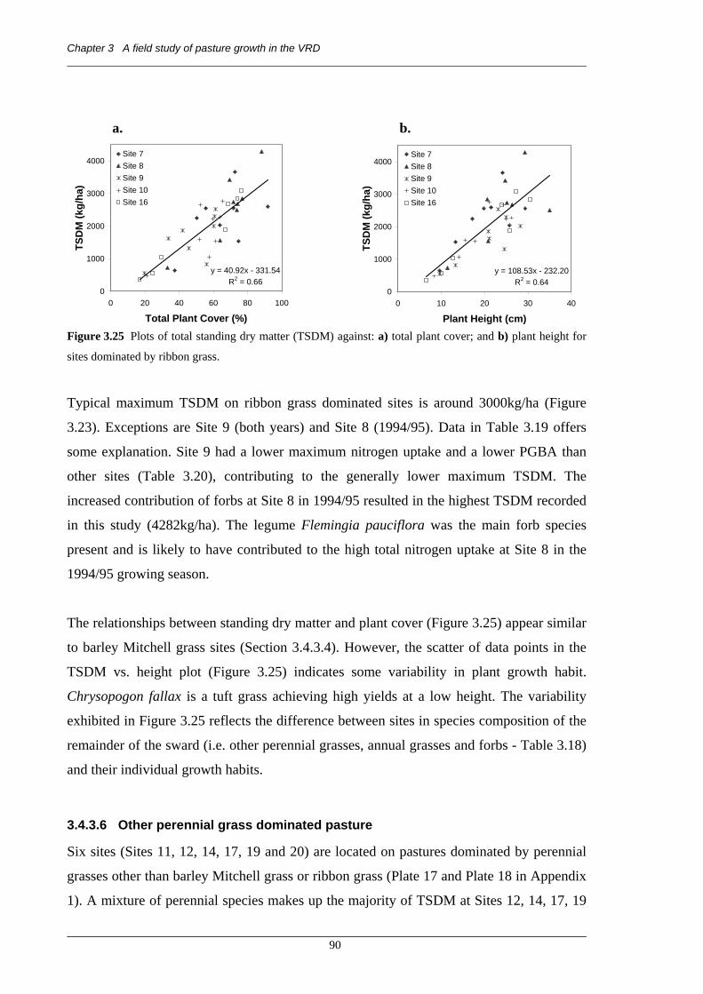
Chapter 3 A field study of pasture growth in the VRD
90
Figure 3.25 Plots of total standing dry matter (TSDM) against: a) total plant cover; and b) plant height for
sites dominated by ribbon grass.
Typical maximum TSDM on ribbon grass dominated sites is around 3000kg/ha (Figure
3.23). Exceptions are Site 9 (both years) and Site 8 (1994/95). Data in Table 3.19 offers
some explanation. Site 9 had a lower maximum nitrogen uptake and a lower PGBA than
other sites (Table 3.20), contributing to the generally lower maximum TSDM. The
increased contribution of forbs at Site 8 in 1994/95 resulted in the highest TSDM recorded
in this study (4282kg/ha). The legume Flemingia pauciflora was the main forb species
present and is likely to have contributed to the high total nitrogen uptake at Site 8 in the
1994/95 growing season.
The relationships between standing dry matter and plant cover (Figure 3.25) appear similar
to barley Mitchell grass sites (Section 3.4.3.4). However, the scatter of data points in the
TSDM vs. height plot (Figure 3.25) indicates some variability in plant growth habit.
Chrysopogon fallax is a tuft grass achieving high yields at a low height. The variability
exhibited in Figure 3.25 reflects the difference between sites in species composition of the
remainder of the sward (i.e. other perennial grasses, annual grasses and forbs - Table 3.18)
and their individual growth habits.
3.4.3.6 Other perennial grass dominated pasture
Six sites (Sites 11, 12, 14, 17, 19 and 20) are located on pastures dominated by perennial
grasses other than barley Mitchell grass or ribbon grass (Plate 17 and Plate 18 in Appendix
1). A mixture of perennial species makes up the majority of TSDM at Sites 12, 14, 17, 19
y = 40.92x - 331.54R2 = 0.66
0
1000
2000
3000
4000
0 20 40 60 80 100
Total Plant Cover (%)
TSD
M (k
g/ha
)
Site 7Site 8Site 9Site 10Site 16
y = 108.53x - 232.20R2 = 0.64
0
1000
2000
3000
4000
0 10 20 30 40
Plant Height (cm)
TSD
M (k
g/ha
)
Site 7Site 8Site 9Site 10Site 16
a. b.

Chapter 3 A field study of pasture growth in the VRD
91
and 20, while Enneapogon polyphyllus is the single dominant perennial at Site 11. While a
full dataset exists for Sites 11, 12 and 19, these have not been included in Figure 3.26 and
Figure 3.27 as results from Sites 14, 17 and 20 span the range of results from all sites in
this group. Data from Sites 11, 12 and 19 not shown here appear in Appendix 6. Cattle
broke into Site 19 at Rosewood during the late dry season of 1996 and consumed all the
pasture. Localised early storms at Auvergne dropped about 200mm of rain on Site 20
before the end of dry season measurements were due, destroying much of the standing dry
pasture. No final measurements were collected from Sites 19 or 20.
Table 3.21 Main pasture and tree species present during the study period for sites dominated by other
perennial grass species.
Site Perennial grasses Annual grasses Forbs Trees Distance to closest tree
11 Enneapogon polyphyllus 1
Aristida inaequiglumis
None present Bonamia pannosa 2
Indigofera hirsuta 2
Carissa lanceolata
Corymbia terminalis
Eucalyptus pruinosa
15m
12 Chrysopogon fallax 1
Dichanthium fecundum 1
Heteropogon contortus 1
Sehima nervosum 1
Brachyachne convergens 2
Dichanthium sericeum
Bonamia pannosa
Gossypium australe 2
Polymeria ambigua 2
Carissa lanceolata
Eucalyptus pruinosa
10m
14 Sehima nervosum 1
Eriachne aristidae 1
Aristida holathera
Heteropogon contortus
Brachyachne convergens Gomphrena canescens 2
Ptilotus exaltatus
Carissa lanceolata
Eucalyptus spp.
Hakea arborescens
Terminalia canescens
10m
17 Dichanthium fecundum 1
Aristida latifolia 1
Brachyachne convergens
Iseilema vaginiflorum
Abutilon otocarpum
Heliotropium tenuifolium 2
Trichodesma zeylanicum
Corymbia terminalis
Terminalia arostrata
20m
19 Sehima nervosum 1
Enneapogon polyphyllus 1
Aristida inaequiglumis
Brachyachne convergens 2
Sporobolus australasicus
Bonamia pannosa
Sida cleistocalyx 2
Corymbia terminalis
Eucalyptus brevifolia
Eucalyptus pruinosa
2 trees within
the site
20 Sehima nervosum 1
Panicum decompositum 1
Dichanthium fecundum 1
Brachyachne convergens
Sorghum spp. 2
Neptunia monosperma
Sesbania cannabina 2
Atalaya hemiglauca
Eucalyptus spp.
Lysiphyllum cunninghamii
Terminalia volucris
10m
1 Most dominant species throughout. 2 Other species abundant at different times.

Chapter 3 A field study of pasture growth in the VRD
92
Figure 3.26 Pasture composition of three sites dominated by other perennial grass species. Error bars
indicate the standard error of the site mean for total standing dry matter at each sampling time (harvest).
Site 14
0
1000
2000
3000
4000
Jul-94 Oct-94 Jan-95 Apr-95 Jul-95 Oct-95 Jan-96 Apr-96 Jul-96 Oct-96
TSD
M (k
g/ha
)
ForbsAnnual GrassPerennial Grass
Site 17
0
1000
2000
3000
4000
Jul-94 Oct-94 Jan-95 Apr-95 Jul-95 Oct-95 Jan-96 Apr-96 Jul-96 Oct-96
TSD
M (k
g/ha
)
ForbsAnnual GrassPerennial Grass
Site 20
0
1000
2000
3000
4000
Jul-94 Oct-94 Jan-95 Apr-95 Jul-95 Oct-95 Jan-96 Apr-96 Jul-96 Oct-96
TSD
M (k
g/ha
)
ForbsAnnual GrassPerennial Grass

Chapter 3 A field study of pasture growth in the VRD
93
Figure 3.27 Pasture nitrogen contents (dashed lines) and nitrogen uptake (vertical bars) of three sites
dominated by other perennial grass species.
The dotted lines represent expected nitrogen contents during periods where no data was collected (explained
in the text at end of Section 3.4.3.4).
Site 14
0
10
20
30
40
50
60
Jul-94 Oct-94 Jan-95 Apr-95 Jul-95 Oct-95 Jan-96 Apr-96 Jul-96 Oct-96
N U
ptak
e (k
g/ha
)
-4.0
-3.0
-2.0
-1.0
0.0
1.0
2.0
3.0
4.0
N C
onte
nt (%
)
Site 17
0
10
20
30
40
50
60
Jul-94 Oct-94 Jan-95 Apr-95 Jul-95 Oct-95 Jan-96 Apr-96 Jul-96 Oct-96
N U
ptak
e (k
g/ha
)
-4.0
-3.0
-2.0
-1.0
0.0
1.0
2.0
3.0
4.0
N C
onte
nt (%
)
Site 20
0
10
20
30
40
50
60
Jul-94 Oct-94 Jan-95 Apr-95 Jul-95 Oct-95 Jan-96 Apr-96 Jul-96 Oct-96
N U
ptak
e (k
g/ha
)
-4.0
-3.0
-2.0
-1.0
0.0
1.0
2.0
3.0
4.0
N C
onte
nt (%
)

Chapter 3 A field study of pasture growth in the VRD
94
Table 3.22 Results for N and P status of pasture at sites dominated by other perennial grass species.
Site Nitrogen Phosphorus
Max. uptake (kg/ha)
Max. content (%)
Min. content (%)
Max. uptake (kg/ha)
Max. content (%)
Min. content (%)
11 17.7 1.73 0.36 1.53 0.084 0.023
12 21.2 1.43 0.54 1.53 0.078 0.028
14 13.0 1.99 0.45 0.68 0.053 0.012
17 15.3 2.00 0.40 1.53 0.160 0.029
19 9.6 2.00 0.46 1.13 0.105 0.046
20 18.3 2.15 0.32 1.17 0.135 0.020
Table 3.23 Some important pasture variables at sites dominated by other perennial grass species.
Site Year PGBA 1
(%)
Peak TSDM 2
(kg/ha)
Growth rate 3
(kg/ha/day)
11 1993/94 2.88 2707 ± 420 14.7
1994/95 2.75 2365 ± 297 13.9
12 1993/94 1.25 2418 ± 366 12.8
1994/95 2.13 3032 ± 477 17.9
14 1994/95 2.88 2396 ± 378 14.2
1995/96 2.13 1581 ± 346 8.6
17 1994/95 3.00 2315 ± 497 15.1
1995/96 1.13 1762 ± 311 9.5
19 1994/95 1.88 1873 ± 677 12.3
1995/96 0.63 736 ± 125 4.0
20 1994/95 0.88 2621 ± 260 17.5
1995/96 2.00 3973 ± 448 20.8
1 PGBA - perennial grass basal area. 2 TSDM- total standing dry matter (± value is the standard error of the site mean). 3 Growth Rate – average daily growth rate calculated using TSDM accumulation from the date of initiation of
growth (Table 3.14) to the end-of-growing-season measurement (Harvest 3).

Chapter 3 A field study of pasture growth in the VRD
95
Figure 3.28 Plots of total standing dry matter (TSDM) against: a) total plant cover; and b) plant height for
sites dominated by other perennial grass species.
Pasture yield in 1994/95 exceeded that in 1995/96 at sites shown in Figure 3.26; however,
at Site 20 this trend is reversed. Examining the associated rainfall data at Kidman Springs
(Site 14), Rosewood (Site 17) and Auvergne (Site 20) - Figure 3.7, Figure 3.11 and Figure
3.13 respectively – reveals that a prolonged dry spell occurred in early 1996 at Kidman
Springs and Rosewood, but was less pronounced at Auvergne. This dry spell brought on
physiological maturity of pasture early and reduced the maximum TSDM (Section 3.4.3.2)
at Sites 14 and 17. Growth was less interrupted at Auvergne and pasture here was able to
take advantage of the high rainfall that occurred late in the 1995/96 growing season.
Species composition varies considerably between sites in this group (Table 3.21), however
the relationship between TSDM and plant height is quite consistent (Figure 3.28). This
may be attributed to most sites containing some mid-height grass species (perennial and/or
annual) and this has resulted in similar TSDM to height relationships across all sites in this
group.
y = 39.88x - 39.05R2 = 0.71
0
1000
2000
3000
4000
0 20 40 60 80 100
Total Plant Cover (%)
TSD
M (k
g/ha
)Site 11Site 12Site 14Site 17Site 19Site 20
y = 110.19x - 596.25R2 = 0.87
0
1000
2000
3000
4000
0 10 20 30 40
Plant Height (cm)
TSD
M (k
g/ha
)
Site 11Site 12Site 14Site 17Site 19Site 20
a. b.

Chapter 3 A field study of pasture growth in the VRD
96
3.4.3.7 Annual short grass dominated pasture
Three sites (Sites 1, 2 and 13) are located on pastures dominated by annual short grass
species (mainly Brachyachne convergens and Sporobolus australasicus - Plate 18 and
Plate 19 in Appendix 1). Each of these sites had a history of preferential grazing for many
years prior to site establishment. The sites in this group represent a species change from
high perennial grass content that occurs on lightly grazed areas, rather than land types
naturally dominated by annual grasses.
Cattle broke into Site 1 during the late dry season of 1995 and consumed all pasture. No
final end-of-dry-season measurement was possible at Site 1.
Table 3.24 Main pasture and tree species present during the study period for sites dominated by annual short
grass species.
Site Perennial grasses Annual grasses Forbs Trees Distance to closest tree
1&2 Aristida latifolia
Enneapogon polyphyllus 2
Brachyachne convergens 1
Sporobolus australasicus 2
Abutilon otocarpum
Indigofera trita
Salsola kali
Sida cleistocalyx 2
Atalaya hemiglauca
Corymbia terminalis
Eucalyptus brevifolia
Grevillea striata
30m
13 Aristida holathera
Aristida latifolia
Enneapogon polyphyllus 2
Brachyachne convergens 1
Dactyloctenium radulans
Bonamia pannosa
Heliotropium tenuifolium 2
Neptunia monosperma
Corymbia terminalis
Eucalyptus pruinosa
20m
1 Most dominant species throughout. 2 Other species abundant at different times.

Chapter 3 A field study of pasture growth in the VRD
97
Figure 3.29 Pasture composition of sites dominated by annual short grass species. Error bars indicate the
standard error of the site mean for total standing dry matter at each sampling time (harvest).
Site 1
0
1000
2000
3000
4000
Jul-93 Oct-93 Jan-94 Apr-94 Jul-94 Oct-94 Jan-95 Apr-95 Jul-95 Oct-95
TSD
M (k
g/ha
)
ForbsAnnual GrassPerennial Grass
Site 2
0
1000
2000
3000
4000
Jul-93 Oct-93 Jan-94 Apr-94 Jul-94 Oct-94 Jan-95 Apr-95 Jul-95 Oct-95
TSD
M (k
g/ha
)
ForbsAnnual GrassPerennial Grass
Site 13
0
1000
2000
3000
4000
Jul-94 Oct-94 Jan-95 Apr-95 Jul-95 Oct-95 Jan-96 Apr-96 Jul-96 Oct-96
TSD
M (k
g/ha
)
ForbsAnnual GrassPerennial Grass

Chapter 3 A field study of pasture growth in the VRD
98
Figure 3.30 Pasture nitrogen contents (dashed lines) and nitrogen uptake (vertical bars) of sites dominated by
annual short grass species.
The dotted lines represent expected nitrogen contents during periods where no data was collected (explained
in the text at end of Section 3.4.3.4).
Site 1
0
10
20
30
40
50
60
Jul-93 Oct-93 Jan-94 Apr-94 Jul-94 Oct-94 Jan-95 Apr-95 Jul-95 Oct-95
N U
ptak
e (k
g/ha
)
-4.0
-3.0
-2.0
-1.0
0.0
1.0
2.0
3.0
4.0
N C
onte
nt (%
)
Site 2
0
10
20
30
40
50
60
Jul-93 Oct-93 Jan-94 Apr-94 Jul-94 Oct-94 Jan-95 Apr-95 Jul-95 Oct-95
N U
ptak
e (k
g/ha
)
-4.0
-3.0
-2.0
-1.0
0.0
1.0
2.0
3.0
4.0
N C
onte
nt (%
)Site 13
0
10
20
30
40
50
60
Jul-94 Oct-94 Jan-95 Apr-95 Jul-95 Oct-95 Jan-96 Apr-96 Jul-96 Oct-96
N U
ptak
e (k
g/ha
)
-4.0
-3.0
-2.0
-1.0
0.0
1.0
2.0
3.0
4.0N
Con
tent
(%)

Chapter 3 A field study of pasture growth in the VRD
99
Table 3.25 Results for N and P status of pasture at sites dominated by annual short grass species.
Site Nitrogen Phosphorus
Max. uptake (kg/ha)
Max. content (%)
Min. content (%)
Max. uptake (kg/ha)
Max. content (%)
Min. content (%)
1 25.5 2.50 0.87 1.78 0.129 0.042
2 23.3 3.13 0.79 1.54 0.125 0.042
13 17.9 2.54 0.69 1.39 0.086 0.024
Table 3.26 Some important pasture variables at sites dominated by annual short grass species.
Site Year AGBA 1
(%)
Peak TSDM 2
(kg/ha)
Growth rate 3
(kg/ha/day)
1 1993/94 8.38 2165 ± 205 10.5
1994/95 1.63 2952 ± 399 21.1
2 1993/94 6.00 1977 ± 239 9.9
1994/95 0.38 2424 ± 263 17.2
13 1994/95 5.75 2593 ± 195 15.2
1995/96 0.38 854 ± 100 4.8
1 AGBA – annual grass basal area. No measurable perennial grasses were present at these sites. 2 TSDM- total standing dry matter (± value is the standard error of the site mean). 3 Growth Rate – average daily growth rate calculated using TSDM accumulation from the date of initiation of
growth (Table 3.14) to the end-of-growing-season measurement (Harvest 3).
Figure 3.31 Plots of total standing dry matter (TSDM) against: a) total plant cover; and b) plant height for
sites dominated by annual short grass species.
Peak pasture TSDM in the annual grass dominated sites (Figure 3.29) appears to be
generally lower than for the perennial grass dominated sites (Section 3.4.3.4 to Section
y = 24.13x + 128.58R2 = 0.62
0
1000
2000
3000
4000
0 20 40 60 80 100
Total Plant Cover (%)
TSD
M (k
g/ha
)
Site 1Site 2Site 13
y = 122.36x - 252.21R2 = 0.82
0
1000
2000
3000
4000
0 10 20 30 40
Plant Height (cm)
TSD
M (k
g/ha
)
Site 1Site 2Site 13
a. b.

Chapter 3 A field study of pasture growth in the VRD
100
3.4.3.6). The major feature of Figure 3.29 is the very low TSDM at Site 13 throughout
1995/96 (maximum TSDM = 854kg/ha). This is likely a result of the combination of two
events. Standard methodological practice (Day and Philp 1997) dictates removal of
standing biomass at the end of the end of the first measurement year. Fire was used to
remove this carryover material. In undisturbed annual short grass pastures, such as at Sites
1, 2 and 13, the seed bank providing next season’s growth is mostly held in the seed heads
of standing pasture. The fire most likely destroyed much of this seed bank, thus reducing
germination and plant density in the second year (Plate 23, Plate 24 and Plate 25 in
Appendix 1). Mott and Andrew (1985) and McIvor et al. (1994) also recognise the
vulnerability of annual grasses to seed bank destruction by fire. In the case of Site 13, the
already-reduced plant density was further hindered by the dry conditions of early 1996
(Figure 3.7). Thus, the combination of these two events resulted in very low pasture
growth at Site 13 in the 1995/96 growing season.

Chapter 3 A field study of pasture growth in the VRD
101
3.4.3.8 Forb dominated pasture
Three sites (Sites 4, 15 and 21) are located on pastures dominated by forb species (Plate 20
and Plate 21 in Appendix 1). Like the annual grass dominated sites, each of these sites
appear to have been preferentially grazed by cattle prior to site establishment. While forbs
are a normal component of native pastures in the region, they are rarely the major
component in unmodified pasture communities. Thus, the sites in this group represent a
species change from the high perennial grass content that occurs on lightly grazed areas,
rather than land types naturally dominated by forb species.
Localised early storms at Auvergne dropped about 200mm of rain on Site 21 before the
end of dry season measurements were due. Much of the dry pasture was destroyed, and
new green growth had occurred by the time the site was accessible. No final measurements
were collected as biomass reflected both new seasons growth and an accelerated
detachment and breakdown rate of the previous season’s growth.
Table 3.27 Main pasture and tree species present during the study period for sites dominated by forb species.
Site Perennial grasses Annual grasses Forbs Trees Distance to closest tree
4 Aristida latifolia 2
Astrebla elymoides
Astrebla pectinata 2
Brachyachne convergens 2
Iseilema fragile
Iseilema vaginiflorum
Abutilon otocarpum 1
Basilicum polystachyon
Rhyncosia australis 1
Trichodesma zeylanicum
Terminalia arostrata 50m
15 Astrebla pectinata 2
Chrysopogon fallax
Aristida latifolia
Astrebla squarrosa 2
Panicum decompositum
Brachyachne convergens 2
Iseilema fragile
Iseilema vaginiflorum
Evolvulus nummalaris
Flemingia pauciflora 1
Neptunia monosperma 1
Rhyncosia minima 1
Sesbania cannabina
None present >500m
21 Chrysopogon fallax 2
Aristida latifolia
Brachyachne convergens 2 Euphorbia schultzii 1
Neptunia monosperma 1
Polymeria ambigua 1
Terminalia volucris
Lysiphyllum cunninghamii
50m
1 Most dominant species throughout. 2 Other species abundant at different times.

Chapter 3 A field study of pasture growth in the VRD
102
Figure 3.32 Pasture composition of sites dominated by forb species. Error bars indicate the standard error of
the site mean for total standing dry matter at each sampling time (harvest).
Site 4
0
1000
2000
3000
4000
Jul-93 Oct-93 Jan-94 Apr-94 Jul-94 Oct-94 Jan-95 Apr-95 Jul-95 Oct-95
TSD
M (k
g/ha
)
ForbsAnnual GrassPerennial Grass
Site 15
0
1000
2000
3000
4000
Jul-94 Oct-94 Jan-95 Apr-95 Jul-95 Oct-95 Jan-96 Apr-96 Jul-96 Oct-96
TSD
M (k
g/ha
)
ForbsAnnual GrassPerennial Grass
Site 21
0
1000
2000
3000
4000
Jul-94 Oct-94 Jan-95 Apr-95 Jul-95 Oct-95 Jan-96 Apr-96 Jul-96 Oct-96
TSD
M (k
g/ha
)
ForbsAnnual GrassPerennial Grass

Chapter 3 A field study of pasture growth in the VRD
103
Figure 3.33 Pasture nitrogen contents (dashed lines) and nitrogen uptake (vertical bars) of sites dominated by
forb species.
The dotted lines represent expected nitrogen contents during periods where no data was collected (explained
in the text at end of Section 3.4.3.4).
The high values in May 1995 at Site 15 are discussed in the text at the end of this section.
Site 4
0
10
20
30
40
50
60
Jul-93 Oct-93 Jan-94 Apr-94 Jul-94 Oct-94 Jan-95 Apr-95 Jul-95 Oct-95
N U
ptak
e (k
g/ha
)
-4.0
-3.0
-2.0
-1.0
0.0
1.0
2.0
3.0
4.0
N C
onte
nt (%
)
Site 15
0
10
20
30
40
50
60
Jul-94 Oct-94 Jan-95 Apr-95 Jul-95 Oct-95 Jan-96 Apr-96 Jul-96 Oct-96
N U
ptak
e (k
g/ha
)
-4.0
-3.0
-2.0
-1.0
0.0
1.0
2.0
3.0
4.0
N C
onte
nt (%
)
Site 21
0
10
20
30
40
50
60
Jul-94 Oct-94 Jan-95 Apr-95 Jul-95 Oct-95 Jan-96 Apr-96 Jul-96 Oct-96
N U
ptak
e (k
g/ha
)
-4.0
-3.0
-2.0
-1.0
0.0
1.0
2.0
3.0
4.0
N C
onte
nt (%
)

Chapter 3 A field study of pasture growth in the VRD
104
Table 3.28 Results for N and P status of pasture at sites dominated by forb species.
Site Nitrogen Phosphorus
Max. uptake (kg/ha)
Max. content (%)
Min. content (%)
Max. uptake (kg/ha)
Max. content (%)
Min. content (%)
4 36.4 2.35 0.85 3.32 0.157 0.049
15 56.4 2.67 0.72 2.64 0.132 0.035
21 19.3 2.55 0.51 0.87 0.174 0.015
Table 3.29 Some important pasture variables at sites dominated by forb species.
Site Year PGBA 1
(%)
Peak TSDM 2
(kg/ha)
Growth rate 3
(kg/ha/day)
4 1993/94 1.00 2343 ± 161 12.5
1994/95 1.00 2950 ± 295 18.9
15 1994/95 0.75 2758 ± 284 17.5
1995/96 1.50 2680 4 13.1
21 1994/95 3.25 2031 ± 172 13.6
1995/96 1.63 1588 ± 111 8.3
1 PGBA - perennial grass basal area. 2 TSDM- total standing dry matter (± value is the standard error of the site mean). 3 Growth Rate – average daily growth rate calculated using TSDM accumulation from the date of initiation of
growth (Table 3.14) to the end-of-growing-season measurement (Harvest 3). 4 No standard error can be calculated for this measurement.
Figure 3.34 Plots of total standing dry matter (TSDM) against: a) total plant cover; and b) plant height for
sites dominated by forb species.
y = 25.81x + 261.44R2 = 0.67
0
1000
2000
3000
4000
0 20 40 60 80 100
Total Plant Cover (%)
TSD
M (k
g/ha
)
Site 4Site 15Site 21
y = 126.07x - 251.44R2 = 0.67
0
1000
2000
3000
4000
0 10 20 30 40
Plant Height (cm)
TSD
M (k
g/ha
)
Site 4Site 15Site 21
a. b.

Chapter 3 A field study of pasture growth in the VRD
105
In Figure 3.33, the May 1995 data for Site 15 is shown as recorded. The nitrogen uptake
value (column) is 56.4kg/ha, far higher (some 20kg/ha higher) than at any other time at this
site or any other site. Such an unusual value requires some investigation to determine
whether it is realistic or contains some error in measurement. Over 2000kg/ha of forbs
were present at this harvest (Plate 21 in Appendix 1), and the sub-sample used to determine
N content was only a small portion of this standing dry matter. While every care was taken
to make this sub-sample as representative as possible, the diversity of forb species present
made this a difficult task. It is conceivable that the sub-sample analysed may have
contained a higher proportion of high N content plant material than was truly
representative. When multiplied by the large dry matter yield, this potential error may have
contributed to the unusually high value shown. Data is reported in this section as collected,
but due to the atypical nature of this value, it is considered an anomaly and omitted when
deriving GRASP model parameters for this site in Chapter 4.
3.5 Discussion of field study results
3.5.1 Climate
Rainfall
Rainfall followed patterns considered typical of the climate in the VRD (e.g. Slatyer 1970).
The first falls were recorded in October or November each year, usually the result of
thunderstorms. These storms are often localised and rainfall received is highly variable and
infrequent. As the growing season progresses, more substantial and sustained falls occur
during December to March resulting from increased storm frequency and waves of
monsoon activity. Daily falls sometimes exceeded 75mm and occasionally more than
100mm was recorded. Rainfall totals were generally close to median values at all study
sites, with some locations receiving well above median rainfall in some seasons (1993/94
at Kidman Springs; 1994/95 at Mt Sanford, Victoria River Downs and Rosewood; and
1995/96 at Victoria River Downs). Short dry periods occurred during the growing season,
with one such period during late January and early February 1996 being the most
significant. Rainfall tended to cease abruptly in March or April, although several isolated
falls after this time were recorded.
One of the most noticeable features of the climate graphs in Section 3.4.1 is the general
gradient in median rainfall, with highest values nearest the coast (Auvergne, Figure 3.14)

Chapter 3 A field study of pasture growth in the VRD ------------------------------------------------------------------------------------------------------------------------------------------ and declining as distance from the coast increases to the furthest inland (Mt Sanford,
Figure 3.6). Variability also increases as median rainfall declines (Table 3.30). This
gradient impacts upon the timing of initiation, duration and cessation of rainfall at
each location (McCown 1981b). This gradient was less pronounced during the
seasons measured in this study as most locations experienced similar rainfall patterns. Table 3.30 Variability in rainfall at the five study locations in the VRD. Rainfall data from DataDrill (2005).
Temperature
The temperature graphs reveal little difference between study locations in either
maximum or minimum temperatures (both the 47-year averages and the values
reported during the study period) throughout the wet season months (November -
May). The dry season months see greater diurnal fluctuations and lower absolute
values for daily maximums and minimums at the more inland locations. Temperatures
during the period of measurement are considered to be close to optimal growth and
the cooler conditions during June to August each year are of little consequence as
pastures are dormant at this time of the year.
Other climate variables
Examination of radiation, evaporation and vapour pressure data (Table 3.4) shows
values during the study period being close to long-term averages. Radiation levels in
the Victoria River District are generally high and are thought not to restrict plant
growth except for short periods during the wet season when heavy monsoonal cloud
cover may persist for several days. These times are associated with the periods of
heavy rainfall as evident in Figure 3.5 to Figure 3.13. Annual potential (Class A pan)
evaporation rates are very high in the VRD; about four times the annual rainfall at
Victoria River Downs. Rainfall exceeds pan evaporation only during a few months of
the year. Thus, the climate in this region is termed semi-arid. Vapour pressure values
were close to long term averages except for
_____________________________________________________________________
106
NOTE: This table is included on page 106 in the print copy of the thesis held in the University of Adelaide Library.

Chapter 3 A field study of pasture growth in the VRD
107
some variation between years in the May to August period (Table 3.4). Plants are dormant
at this time of year and variation in vapour pressure has no impact on plant growth.
3.5.2 Soils
Soil bulk density
Soil bulk density (BD) reported by Day (1977) on red earths are close to those measured
on comparable sites in this study (Table 3.6 and Table 3.8), ranging from 1.4 - 1.5g/cm3 at
the surface to 1.5 - 1.8g/cm3 at depth. Lodge et al. (2003b) found BD values of 1.4g/cm3 at
the surface and 1.6 to 1.7g/cm3 below 40cm depth in a red Chromosol soil in northern
NSW. Bulk density values for cracking clay sites in this study are similar to or higher than
published data. Dalgliesh and Foale (1998) provide BD values for black vertosols of 1.0 -
1.2g/cm3 at the surface and 1.2 - 1.4g/cm3 at 1.0m.; and grey vertosols have BD’s in the
order of 1.4 – 1.6g/cm3 and changing little throughout the profile. The cracking clay soils
(vertosols) in this study have measured bulk densities of about 1.3g/cm3 and 1.5g/cm3 near
the surface, and about 1.65g/cm3 and 1.7g/cm3 at depth for basalt and alluvial clays
respectively (Table 3.31). These denser soil profiles contribute to the higher water holding
capacities of soils in this study than in the published data. Berndt and Coughlan (1976)
note some issues with measuring bulk density of cracking clay soils using small-diameter
core-sampler such as used in this study (Plate 8 in Appendix 1), as bulk density varies with
water content due to shrinkage and swelling of the soil being three-dimensional (Talsma
and van der Lelij 1976; Smiles 1997).
Soil water content
Slatyer (1954) estimated plant available water holding capacity (WHC) of 85mm/m on the
red limestone soils (Tippera) surrounding Katherine. This value is much less than the
values found for similar soils as part of this study. Day (1977) reported red earth soils with
WHC’s of 77 to 135mm/m in the Daly Basin, north-east of the VRD. The WHC’s of red
earths measured in this study (mostly 120 to 150mm/m, Table 3.6 and Table 3.8, averaging
139mm/m, Table 3.31) are at the upper end of the values reported by Day 1977.
The highest values of WHC for this study were found on the cracking clays overlying
basalt (Table 3.10 and Table 3.31). Mott et al. (1985) give some average values for WHC
in self-mulching cracking clays of 220mm/m, values similar to those reported by McKeon

Chapter 3 A field study of pasture growth in the VRD
108
et al. (1990). Dalgliesh and Foale (1998) list water holding capacities of 150 to 250mm/m
and Hochman et al. (2001) report WHC’s of 124mm/m for black vertosols (similar to
basalt clays), compared to 215 to 315mm/m measured here. Dalgliesh and Foale (1998)
also quote WHC’s of 130 to 200mm/m and Hochman et al. (2001) report WHC’s of
101mm/m on grey vertosols (similar to alluvial clays), compared with the measured values
in this study of 150 to 280mm/m (Table 3.12). Taddese et al. (2002) measured water
holding capacity of 140mm/m in a vertosol soil in Ethiopia.
Determining WHC from field measurements is difficult (Dalgliesh and Foale 1998),
particularly for the cracking clays (Greacen and Williams 1983; Isbell 1983; Dalgliesh et
al. 1998). Isbell (1983) comments that “application of arbitrary upper and lower limits
based on water contents derived from the moisture characteristic are of limited value in
describing the water store of a cracking clay”. The nature of cracking clay soils is such
that once the soil profile is full, drainage is slow and true drained upper limit is difficult to
assess. The highest soil water contents encountered during this study (cracking clays
overlying basalt, Figure 3.17) were all measured some 7 days after the last rain, and yet
conditions were sometimes still boggy and sites difficult to access. It is conceivable that
some of the high soil water values assumed to be ‘field capacity’ may in fact still be
saturated. A more accurate estimate of field capacity would require detailed measurement
of soil water content and soil water potential as the soil dries from ‘saturated’ to ‘field
capacity’. Given the broad scale and remote nature of the current study, it was not possible
to make these more detailed measurements. The soil data presented is the most detailed
available for VRD soils.
Wilting point in cracking clays can also be problematic to ascertain. Their cracking nature
results in soil water loss by evaporation directly from the deep cracks, lowering the soil
water content in the soil surrounding the cracks to below true wilting point. Thus, sampling
results can vary from hole to hole at the same site, depending on whether the sample is
collected from the middle of a large ped, or closer to the ped edge.
The red earth soils are easier to measure for WHC due to their higher position in the
landscape (better drainage) and lower clay content making them easier to traverse.
However, the isolated location of many of the sites meant access to them required crossing

Chapter 3 A field study of pasture growth in the VRD
109
watercourses and cracking clay soils and, therefore, sampling was sometimes not possible
at the wettest times of the year.
Another potential contributing factor to the higher WHC’s reported here is plant root
density. Baker and Ahern (1989) emphasise that “estimates of rooting depth are necessary
parameters in predicting available water capacity of soils”. Isbell (1983) and Hochman et
al. (2001) discuss the impact of plant root patterns on wilting point values when
determining WHC, suggesting that fibrous-rooted and tap-rooted plants will have different
wilting points in the same soil. Similarly, annual crops will have different wilting points to
perennial plants. One feature of the soil water charts presented in this chapter is the relative
uniformity of soil water availability down the soil profile. Established perennial grass
plants on undisturbed soils are likely to have greater root density deep in the soil profile
than the annually cropped soils that are the source of some published WHC data. Greater
root density results in a higher level of water extraction and therefore lowers the effective
wilting point. Low wilting point values contribute to the higher total WHC’s presented
here in comparison to those reported in the literature.
Table 3.31 Summary of results for important soil variables.
Soil bulk density (g/cm3) Water Holding Capacity
Soil group Assumed pasture rooting depth
0-10cm 50-60cm 80-90cm Total (mm)
Average (mm/m)
Red earths – basalt 1.0m 1.50 1.56 1.56 145.7 145.7
Red earths – limestone 0.6m 1.58 1.65 - 83.4 138.9
Cracking clays – basalt 0.9m 1.30 1.55 1.64 277.3 308.1
Cracking clays - alluvial 1.0m 1.52 1.66 1.73 231.7 231.7
Soil chemistry and nutrients
Soil chemistry and nutrient analyses were restricted to the top 20cm of soil, as this zone
contains the most organic matter (Spain et al. 1983) and greatest concentrations of the
major elements (Christie 1979). Organic carbon content of the soils in this study ranged
from 12752kg/ha to 26771kg/ha in the top 20cm of soil (Table 3.32) (0.5% – 1.1%, Table
9.5 to Table 9.8), values within the range given by Spain et al. (1983) for these soil types.
Total soil nitrogen contents were 650kg/ha to 1222kg/ha in the top 20cm (0.02% – 0.04%),
values much lower than those of Spain et al. (1983) and Mott et al. (1985), but similar to

Chapter 3 A field study of pasture growth in the VRD
110
the results of Christie (1979). Nitrate nitrogen levels were extremely low, ranging from
3.1kg/ha to 4.3kg/ha (1.1 – 1.4 ppm) in the top 20cm. Total phosphorus levels were also
very low at 303kg/ha to 679kg/ha (0.010% – 0.023%), similar to the ‘infertile sandy red
earth’ studied by Christie (1979).
Chemical properties for red earths, and to a lesser extent cracking clays, have been
reported for nearby regions. In general, reported values for base exchange capacity and
total and exchangeable N, P, S and K that are similar or less than those recorded in Table
9.5 to Table 9.8. The red earths in the Daly Basin (Day 1977) were slightly acid (pH 5.7 –
6.7) as were those at Katherine (Williams et al. 1985), while similar soils in this study are
neutral to slightly alkaline (pH 7.2 – 8.4). Williams et al. (1985) report a cracking clay soil
as slightly alkaline (pH 8.0), consistent with results here (Table 9.7 and Table 9.8).
Table 3.32 Summary of soil chemistry results for each of the major soil types in this study.
Soil type pHwater OC 1 NO3-N 2 N(t) 3 P(bicarb) 4 P(t) 5 C:N ratio 6
Red earths – basalt 7.5 18603 3.4 1081 18.5 679 17.2
Red earths – limestone 7.7 26771 4.3 1222 32.0 605 21.9
Cracking clays – basalt 8.1 12752 3.1 650 22.0 305 19.6
Cracking clays - alluvial 8.1 15643 4.3 756 19.2 303 20.7
1 OC - organic carbon; 2 NO3-N – nitrate nitrogen; 3 N(t) - total nitrogen; 4 P(bicarb) – bicarbonate
extractable (Colwell); 5 P(t) - total phosphorus; 6 C:N ratio – carbon to nitrogen ratio. All units are kg/ha in
the top 20cm of soil, except the pH and C:N ratio, which are dimensionless.
Summary
Results from this study indicate that soils in the VRD have generally higher plant available
water capacities than those reported for comparable soils in other regions. Cracking clay
soils of basalt origin have higher water holding capacities than soils of alluvial origin. The
shallow red earths have the lowest WHC’s. The studied soils contain similar levels of
many nutrients as those in the literature, except for the cracking clay soils, which contained
lower amounts of total nitrogen than published data. As with most soils in Australia’s
semi-arid tropics, natural fertility levels are very low, particularly deficient for N and P.
These low levels of N and P have been identified as a major constraint to pasture growth in
the VRD (Mott et al. 1985).
Chapter 3 A field study of pasture growth in the VRD
111
Overall, the soils measured in this study possess physical and chemical properties that are
(with the exception of the high field capacities) essentially similar to comparable soils in
other regions of northern Australia. Much of the data presented in this chapter and in
Appendix 3 are the first of their kind to be published for the VRD.
3.5.3 Pastures
Observations of species dynamics
At some sites, species composition and phenology varied throughout the study period.
Such variations were probably due to either exclosure from grazing, prevailing seasonal
conditions, response to fire after burning to remove carryover material, seasonal variations
in nutrient supply, inter-plant competition, or some combination of these factors. While a
general understanding exists of how these factors affect pasture communities, the
individual species-specific responses are not well understood.
Many studies have examined the biology and ecology of individual native grass and forb
species in northern Australia (e.g. Norman 1963b; Mott 1978; Jacobsen 1981; Hacker
1984; Andrew 1986; Cook and Andrew 1991; Orr 1991; Stockwell et al. 1994). These
studies have provided a good understanding of many species and an overall general
appreciation for the factors influencing pasture species dynamics. However, observations
during this study noted a variety of responses, some of which are inconsistent with these
published works. Some gaps in knowledge were also revealed. Suggested further research
to improve our understanding of the pasture system includes: nitrogen fixation by common
legumes such as Flemingia pauciflora, Rhyncosia minima and Neptunia monosperma; the
germination and emergence of Dichanthium sericeum, Iseilema vaginiflorum and similar
mid height grasses under field conditions in the VRD; and the seed bank dynamics of
annual short grasses such as Brachyachne convergens and Sporobolus australasicus and
how they are affected by fire.
Total standing dry matter
Maximum total standing dry matter (TSDM) across all sites and years varied from 736 to
4282kg/ha. Throughout this study the highest mean maximum TSDM values were
measured on sites dominated by perennial grasses, followed by forb sites, with annual
grass dominated pastures having the lowest (Table 3.33). TSDM’s of pastures in this study

Chapter 3 A field study of pasture growth in the VRD
112
are generally consistent with those reported by Foran et al. (1985) (800 to 2100kg/ha),
McIvor et al. (1994) (1490 to 2240kg/ha), MacDonald et al. (1997) (1530 to 2560kg/ha)
and Bastin et al. (2003) (1700 to 3000kg/ha), albeit at the upper end of the ranges they
provide (Table 2.2). This is mainly attributable to the favourable seasonal conditions that
prevailed during the study period, the high water holding capacity of the soils, and the
absence of trees and grazing on the sites measured.
In the annual short grass dominated sites, burning the undisturbed pasture to remove
carryover material at the end of the first study year (Sites 1 and 2 in 1994, and Site 13 in
1995) is suspected of destroying much of the seed bank needed for the following season.
Germination was sparse and few individual plants grew during the second study year at
these sites (Table 3.26). While end of growing season TSDM in 1995 was not reduced at
Sites 1 and 2, this was a season of above median rainfall. Site 13, however, shows
drastically reduced growth in the second study year (Figure 3.29), a season of
approximately median rainfall during which periods of hot and dry weather affected plant
growth. These observations highlight the vulnerability of pastures containing high
proportions of annual species to fire and less than favourable seasonal conditions.
Table 3.33 Summary of field results for important pasture variables.
Species PGBA 1 (%)
Max. TSDM 2 (kg/ha)
Max. N uptake (kg/ha)
Max. N content
(%)
Min. N content
(%)
Barley Mitchell grass 2.85 2851±141 24 1.96 0.48
Ribbon grass 2.96 2970±117 24 1.74 0.50
Other perennial grasses 1.96 2315±135 15 1.66 0.50
Annual short grasses 0.02 2161±136 19 2.27 0.88
Forbs 1.52 2392±111 30 2.37 0.77
1 PGBA - perennial grass basal area.
2 TSDM- total standing dry matter (± value is the standard error of the group mean).
Measuring TSDM introduces the issue of measurement variance. Variance occurs because
of spatial heterogeneity in native pasture communities; that is, pasture density differs
considerably over short distances. Section 3.3.5 details the methodology used in this study
for collecting TSDM data, prescribing eight individual measurements that are averaged to
provide a mean value of TSDM for each site at that harvest. Results from the field study

Chapter 3 A field study of pasture growth in the VRD
113
show considerable spatial variation in TSDM at many sites throughout the growth cycle.
This variation is illustrated by the relatively large standard error bars in Figure 3.20, Figure
3.23, Figure 3.26, Figure 3.29, and Figure 3.32; and in the individual TSDM results in
Table 9.12 (Appendix 7).
Table 3.34 summarises measurement variance for TSDM in this study, represented by 95%
confidence limits about the harvest mean (Goldman and Weinberg 1985). Early wet season
measurements display greater variance that at any other time. Overall, measurement
variance was ±35.4% of the TSDM harvest mean, indicating that many pasture yield
results contain sizeable statistical error. This level of measurement variance in the field
data becomes important when evaluating modelling results in Chapter 4 and Chapter 5.
Table 3.34 Variance in field measurements of total standing dry matter (TSDM) for 21 sites over two years.
Values represent 95% confidence limits expressed as a proportion of the harvest mean.
n Minimum 95% confidence limit value for 21
sites over two years
Maximum 95% confidence limit value for 21
sites over two years
Mean 95% confidence limit value for 21
sites over two years
Early wet (H1 and H5) 42 ±16.7% ±162.2% ±44.8%
Mid wet (H2 and H6) 42 ±4.5% ±89.4% ±30.6%
End of wet (H3 and H7) 42 ±7.0% ±85.5% ±30.4%
End of dry (H4 and H8) 37 ±13.5% ±102.4% ±35.8%
All data 163 ±35.4%
Data summarised from Table 9.12. H1 is harvest 1, and so on.
Perennial grass basal area
Perennial grass basal area (PGBA) measured during this study varied from 0.0 - 6.0% of
the soil surface, with most values between 2 - 3%. Mott et al. (1985) report a typical value
of around 4% for Australian savannas with the inter-tussock spaces supporting a wide
variety of ephemeral grasses and forbs. Observations of basal area made during this study
are consistent with Mott et al. (1985), and a number of other studies in northern Australia.
A study on native pastures on northern Western Australia by Holm and Eliot (1980)
recorded PGBA on cracking clays of 2.96%; and another study on the Barkly Tableland by
Foran and Bastin (1984) also found PGBA values similar to those in this study (1.0 –

Chapter 3 A field study of pasture growth in the VRD
114
4.0%). Foran et al. (1985) report total basal cover (annuals plus perennials) of 0.06 –
3.39% in pastures on red earths at Kidman Springs.
McIvor et al. (1995a) report a positive relationship between PGBA and TSDM on tropical
tall-grass pastures near Katherine. Results from this study show a similar trend, although
the relationship is poor (y = 207x + 2143, r2 = 0.171, Figure 3.35c). Not surprisingly, as
PGBA increases so does perennial grass production (y = 457x + 512, r2 = 0.534, Figure
3.35a), and sites dominated by perennial grasses have highest TSDM (Table 3.33). Foran
and Bastin (1984) report similar findings on Mitchell grass pastures in the Barkly
Tableland. Conversely, as PGBA increases the production of annual grasses and forbs
declines, but the relationship is less pronounced (y = -250x + 1630, r2 = 0.248, Figure
3.35b). TSDM of annual grasses and forbs is more likely related to factors other than
PGBA, such as seed bank density, nutrient availability and evapotranspiration.
Reduction in PGBA by grazing results in species composition change, with perennial
grasses declining and annual grasses and forbs increasing in abundance (Gardener and
McIvor 1985). Observations in this study suggest that soil type is influential on how
species change is exhibited. Low PGBA on red earth soils results in dominance of the
sward by annual short grasses. However, on cracking clays, forbs are the main contributor
to total biomass when perennial grasses are sparse.

Chapter 3 A field study of pasture growth in the VRD
115
Figure 3.35 Relationships between perennial grass basal area (PGBA) and end of growing season standing
dry matter (SDM) of a) perennial grasses; b) annual grasses and forbs; and c) total pasture.
Nutrients
End of growing season total plant nitrogen uptake varied from 9.6kg/ha to 56.4kg/ha, and
nitrogen content varied from 0.32% to 3.13%. The highest total N uptake and N content
values recorded in this study occur on forb dominated sites and annual grass dominated
sites respectively (Table 3.28 and Table 3.25). Friedel (1981) reports nitrogen levels in
combined herbage and litter of 30 to 72kg/ha, while Ash and McIvor (1995) report 5 to
21kg/ha of nitrogen uptake in tropical tallgrass pastures depending on pasture condition.
They also report an increase in plant N concentration as the proportion of annual grasses
and forbs in a pasture sward increase. Schmidt et al. (1998) also found that annual species
have a high capacity for nitrogen assimilation. Many forbs are legumes and supplement
soil-available N by fixing nitrogen from the atmosphere, thus increasing the total N supply
available for growth (Peoples and Baldock 2001). No data is available on the contribution
y = 207x + 2143R2 = 0.171
0
1000
2000
3000
4000
5000
0 1 2 3 4 5 6
PGBA (%)
Tota
l pas
ture
SD
M (k
g/ha
) Total SDMn = 42
c.
y = -250x + 1630R2 = 0.248
0
1000
2000
3000
4000
5000
0 1 2 3 4 5 6
PGBA (%)
Ann
ual g
rass
es a
nd fo
rbs
SDM
(kg/
ha)
Annual Grasses andForbs SDM
n = 42
b.y = 457x + 512
R2 = 0.534
0
1000
2000
3000
4000
5000
0 1 2 3 4 5 6
PGBA (%)
Pere
nnia
l gra
ss S
DM
(kg/
ha)
PerennialGrass SDM
n = 42
a.

Chapter 3 A field study of pasture growth in the VRD
116
of native legumes to plant N supply in the VRD, but results of this study suggest they
contribute to the total supply of N available for plant growth.
Results of nitrogen uptake during the growing season show a rapid increase in total plant
nitrogen yield during the early to mid wet season, then little further increase for the
remainder of the growing season (e.g. Figure 3.21). This pattern is consistent with Christie
(1981) who reports nitrogen uptake rates declining rapidly after 8 continuous weeks of
growth in a Mitchell grassland in Queensland.
The lowest values for minimum N content occur in perennial grass pastures (Table 3.33).
This implies that perennial grasses are able to continue growth after soil N supply is
exhausted by internally diluting nitrogen to a lower concentration than can annual grasses
and forbs. In an environment where soil nutrients are often a major limit to pasture growth
(Section 2.3.2), internal N dilution is influential on end of growing season TSDM. Christie
(1981) reports higher conversion efficiency of nitrogen into pasture biomass by a perennial
C4 grass than for other species under the same conditions, supporting the results of this
study. Hendricksen et al. (1992) and Holm and Eliot (1980) both report declining plant N
concentration as the growing season progresses, findings also consistent with results of this
study.
Summary of field study
• seasonal rainfall totals (July - June) recorded in the study varied from 538mm to
1062mm, being influenced by location and by year. All sites received rainfall totals
near to, or well above, long-term medians (34th to 97th percentiles);
• plant available water capacity of soil profiles varies from 123mm/m to 350mm/m and
is a function of soil texture, soil depth, drainage and plant rooting pattern. These values
are similar to, or greater than, other published data from comparable soil types;
• soil fertility, as reflected in the soil nutrient and chemical properties, indicates these
soils to be typical for the northern Australian rangelands. Available nitrogen and
phosphorus are generally extremely low for much of the year;
• Pasture species composition at any individual location can vary from year to year
depending upon grazing pressure, prevailing seasonal conditions, fire, available

Chapter 3 A field study of pasture growth in the VRD
117
nutrient supply, and competition with other species. Some of these responses are not
well understood;
• maximum pasture TSDM varies from 736kg/ha to 4282kg/ha and is influenced by
location, year, soil type, plant density, species composition, and nutrient supply and
dilution;
• TSDM measured using the Swiftsynd methodology results in variance of ±35% of the
mean, and this becomes important during the modelling process in the following
chapters;
• perennial grass based pastures generally have highest TSDM (average of 2712kg/ha),
and annual species (grasses and forbs) are more prone to variations in abundance due to
seasonal conditions and/or management (e.g. burning); and
• Nitrogen supply increases with content of annual grasses and forbs, but this is offset by
a lower efficiency at converting N into plant biomass.
3.6 Conclusions
The field study results presented in this chapter provide comprehensive detail for a range
of land types on the climatic conditions, soil properties and resulting pasture responses
during the study period. Rainfall and other climate variables during the study period were
generally favourable for pasture growth and, apart from a dry period during one growing
season, no effect of drought or other extreme weather was experienced.
Soil water holding capacity is dependent on soil type, and WHC’s of soils in this study
were generally high compared to other published data from comparable soils. This
difference is attributed to high soil bulk density and the increased soil water extraction of
established perennial grasses compared with the annually-cropped soils that are the source
of much of the published water holding capacity data. Levels of soil nitrogen and
phosphorus are naturally very low.
Pasture biomass production is similar to, or higher than other studies in and around the
VRD. Two main factors contribute to this result:
• pastures in this study were measured without the effect of grazing or the presence of
trees, both which reduce pasture biomass accumulation; and

Chapter 3 A field study of pasture growth in the VRD
118
• the favourable growing conditions resulted in a considerable contribution of annual
grasses and forbs to total pasture production, even on perennial-dominated pasture
types.
A number of limitations in the accuracy of the field data have been revealed:
• determining soil water holding capacity of cracking clay soils from field measurements
is difficult, and the isolated nature of the study sites has exacerbated this problem;
• the methodology employed to measure pasture biomass has resulted in sizeable
measurement error due to the spatial heterogeneity of pasture types in the VRD; and
• plant nitrogen uptake is also subject to some error due to difficulty in obtaining
representative subsamples in cases where pastures contain high biomass with many
species.
It is concluded that, with some noted exceptions, the dataset produced as a results of this
field study is suitable for developing local values for input parameters of the GRASP
pasture growth model. In addition, the dataset represents the most detailed description of
soil water capacity, pasture growth and N uptake yet assembled for the VRD.

Chapter 4 Analysis of field measurements using a systems modelling approach
119
4.0 Analysis of field measurements using a systems modelling approach
4.1 Introduction
Analysis of real systems using simulation modelling involves a number of phases. Grant et
al. (1997) identify four phases of systems analysis:
• conceptual model formulation (abstracting from the real system to develop a
conceptual, qualitative model of the system of interest);
• quantitative model specification (development of the mathematical equations and their
parameter values that collectively form the quantitative model);
• model evaluation (the process of determining the relative usefulness of a model for
meeting specific objectives); and
• model use (answering the questions that were identified at the beginning of the
modelling project).
The four phases of systems analysis are highly interconnected and model development may
cycle through several phases more than once. The GRASP pasture growth model has
already passed through the model evaluation and use phases numerous times and is
therefore considerably robust in structure for the environments in which it has been
developed and applied. However, GRASP has not yet been evaluated under the unique
conditions of the VRD.
This chapter aims to calibrate the GRASP model on a site-by-site and year-by-year basis
using the field data reported in Chapter 3, and assess the performance of the model when
predicting key soil and pasture variables. To achieve this aim, Section 4.2 first provides an
overview of the GRASP model to provide the reader with an understanding of the model
structure and the need to derive values for a number of important parameters. While the
actual calibration process partially depends on characteristics of the site where field data
was collected, it is an essentially systematic procedure, and the general approach is
described in Section 4.3. The individual site and season parameter values resulting from
calibration are presented in Section 4.4. GRASP’s ability to mimic the pasture system at
the field study sites is assessed by comparison of model output with field data for several
key variables (i.e. standing dry matter, soil water content, nutrient uptake and plant cover)
the results of which are presented in Section 4.5. The capability of the model and its

Chapter 4 Analysis of field measurements using a systems modelling approach
120
limitations are discussed in Section 4.6 and conclusions presented in Section 4.7. Figure
4.1 illustrates the structure of this chapter and Figure 4.2 shows the phases of systems
analysis and model development, and how the components of this study relate to each
phase.
Figure 4.1 The structure of Chapter 4.
Figure 4.2 The four phases of systems analysis (bolded text in box) and an indication of where the
components of this study fit within this framework (after Grant et al. 1997).
Conceptual model formulation
Quantitative model specification
Model evaluation
Model use
Collection of local field data – Chapter 3
Calibration of model from field results – Chapter 4
Sensitivity testing of model to determine factors most influential on pasture growth – Chapter 6 Application of model to management of grazing land in the VRD – Chapter 7
Validation of model with independent data to test its capability – Chapter 5
Overview of the calibration procedure (Section 4.3)
Derive GRASP parameters that describe each individual site (Section 4.4)
Overview of the GRASP model (Section 4.2)
Assessing the fit between model results and field data
(Section 4.5)
Discussion and conclusions (Section 4.6 and Section 4.7)

Chapter 4 Analysis of field measurements using a systems modelling approach
121
4.2 An overview of the GRASP pasture growth model
The GRASP model is documented by McKeon et al. (1990) and in more detail by
Littleboy and McKeon (1997). A simplified version including the rationale of many
components is provided by Rickert et al. (2000). The core of the model, ‘Subroutine
GRASP’, has remained largely unchanged since the early 1990’s and is the focus of this
overview. Many developmental versions based upon Subroutine GRASP now exist.
‘Spaghetti GRASP’ is Dr Greg McKeon’s most advanced form of GRASP, and a
personalised copy, ‘GVT89MQ3’ is used in this study (G.M. McKeon pers.comm.).
The objective of the GRASP model is to simulate the soil water balance, pasture growth
and other important biophysical processes by using data from short-term field observations
and extrapolating over many years. Outputs from the model can then be used in decision-
making processes by researchers, policy makers and grazing land managers. Day et al.
(1993) state that a fundamental step in providing recommendations for pasture
management is to assess likely spatial and temporal variability in pasture production. The
limited availability of pasture productivity data in most cases means assessments of such
variability can only be made by extrapolating from long-term climatic data in association
with estimates of site productivity.
In GRASP, pasture growth is related to transpired water by a model parameter termed
‘transpiration-use-efficiency’ (TUE). Transpiration is a component of the formal water
balance calculated by GRASP (Figure 2.6). Pasture growth is assumed to be directly
proportional to the rate of transpiration (Arkley 1963; Rose et al. 1972; Tanner and
Sinclair 1983; Walker and Richards 1985). Calculating transpiration-use-efficiency
requires knowledge of plant growth and soil water. This is the basis for data collection in
the field study reported in Chapter 3.
4.2.1 Soil water balance
The soil water balance is simulated using three soil layers (0 - 10cm, 10 - 50cm, 50cm to
pasture rooting depth (assumed maximum depth is 100cm). Studies of pasture in northern
Australia report low root densities in the soil profile below one metre (McCown 1971;
Christie 1978; Christie 1981). A fourth layer (grass rooting depth to tree rooting depth) can
be simulated but is not incorporated in this study as the focus is on pasture rather than

Chapter 4 Analysis of field measurements using a systems modelling approach
122
trees. The processes of runoff, infiltration, drainage, soil evaporation and transpiration are
calculated separately for each day from inputs of rainfall and pan evaporation. Surface
cover, rainfall intensity and soil moisture are part of the runoff calculation (McIvor et al.
1995b; Scanlan et al. 1996b; Owens et al. 2003). Runoff relationships apply to mid-slope
locations. Little quantitative data exists for deep drainage in northern Australian
rangelands, but Harrington et al. (1984) and Christie (1981) suggest that evaporation and
transpiration are the main pathways of rainfall, and drainage is low in semi-arid rangelands
(except under prolonged saturation, Talsma and van der Lelij 1976). Lodge et al. (2003a)
also found that evapotranspiration was the largest output term in the soil water balance of a
native pasture in New South Wales, and that runoff and drainage were episodic events.
The water balance equation is given by Rickert et al. (2000):
SWt = SWt-1 + Raint + Irrigt - Draint - Runofft - Esoilt - Transt – Ecanopyt - Elittert
(Equation 8)
where SWt and SWt-1 are the soil water contents for t and t-1 days respectively, and Raint,
Irrigt, Draint, Runofft, Esoilt, Transt, Ecanopyt and Elittert are daily flows of rainfall,
irrigation, deep drainage, runoff, soil evaporation, transpiration, canopy interception and
litter interception respectively. All components must be in the same units (i.e. millimetres).
In this study, irrigation and canopy interception are of little relevance (no sites were
irrigated and only one site contained trees). Rickert et al. (2000) state that locations with a
high proportion of rainfall events of less than 25mm may experience substantial
evaporative losses by water adhering to surface litter. In tropical northern Australia, a high
proportion of rainfall received comes from heavy storms (e.g. 44% of total seasonal
rainfall at Victoria River Downs Station comes in falls exceeding 25mm - DataDrill 2005),
thus minimising the influence of evaporation from litter on the soil water balance. With
these factors having minimal influence in this study, the main factors contributing to
variation in the soil water balance are rainfall, runoff, evaporation and transpiration.
Drainage will be important in very wet periods, but no data is available for the region.
Calculating the soil water balance:
• recorded daily rainfall is partitioned into runoff and infiltration;

Chapter 4 Analysis of field measurements using a systems modelling approach
123
runoff is estimated using relationship derived from Scanlan et al. (1996a), and has
recently been improved using a ‘curve number runoff method’ (Owens et al. 2003).
Runoff is affected by cover (high cover = low runoff), soil water deficit (dry soil =
low runoff), and rainfall intensity (high intensity = high runoff). Slope is a factor in
the runoff calculation but most simulations assume a gentle gradient;
water not run off is infiltrated into the surface layer;
• when trees are present, tree basal area is used to determine transpiration by trees from a
set relationship (Calder 1992). At a tree basal area of 20m2/ha transpiration from trees
will equal pan evaporation;
• pasture transpiration is calculated from green plant cover, pan evaporation and vapour
pressure deficit. It has priority of water use over soil evaporation;
• soil evaporation occurs in the 0 - 50cm (mostly 0 - 10cm) layers, and is inversely
related to surface cover. Evaporation from the soil surface decreases as surface water
contents decrease (Eastham et al. 1992). Consideration is given to the cracking soils
where some moisture loss directly from the 50 - 100cm layer occurs through
evaporation;
• infiltration from one soil layer to the next occurs when soil water content exceeds the
field capacity of that layer; and
• deep drainage is estimated from the amount of soil water above field capacity in the
deepest soil layer for pasture growth (i.e. 50 - 100cm).
4.2.2 Pasture growth, death, detachment and breakdown
Once the soil water balance (Equation 8) has been quantified and transpiration by pasture
has been calculated from green cover and available soil water, the processes of pasture
growth, death and detachment can be quantified (McKeon et al. 1982b). In ideal conditions
pastures grow at a potential rate determined by their physiology. Under variable
conditions, growth is constrained by supply of soil water, ambient temperature, solar
radiation, and nutrient supply (Rickert et al. 2000).
Pasture growth is determined for water limiting and radiation limiting conditions, with the
most limiting factor determining growth (Littleboy and McKeon 1997). Under water
limiting conditions, growth is calculated from transpiration and transpiration-use-
efficiency (dry matter accumulation per unit of transpiration). Under radiation limiting

Chapter 4 Analysis of field measurements using a systems modelling approach
124
conditions, growth is calculated from intercepted radiation and radiation-use-efficiency
(dry matter accumulation per unit of radiation). Growth occurs within constraints of
nitrogen availability and temperature. The nitrogen availability function (Figure 4.3)
assumes some N is stored internally (perennial roots or seeds), and uptake of N per unit of
transpiration is constant until transpiration ceases due to soil water limitations or a user-
defined maximum amount of available N has been reached. Calculation of regrowth from
stored reserves is required when little or no green material is present to transpire water or
intercept radiation (i.e. after plant dormancy or defoliation by grazing or fire).
Figure 4.3 Relationship between accumulated pasture transpiration and nitrogen uptake (from Littleboy and
McKeon 1997). The user-defined coefficients for stored plant N reserves, N uptake per 100mm of
transpiration, and maximum N available for uptake shown in this figure are realistic for the semi-arid tropics,
but are examples only.
Dry matter is simulated in three biomass pools: green, dead, and litter (detached dead); and
the processes of growth, death, and detachment transfer biomass from one pool to another
(Figure 2.6 and Figure 4.4). Biomass in the green pool is partitioned into leaf and stem
pools via a user-defined ratio. Breakdown of litter returns dry matter to the soil. Soil
organic matter dynamics are not simulated by GRASP.
0
10
20
30
40
50
0 100 200 300 400 500 600 700 800 900 1000
Accumulated transpiration (mm)
Nitr
ogen
upt
ake
(kg/
ha)
Stored plant N reserves = 5kg/haN uptake per 100mm transpiration = 5kg/haMaximum N available for uptake = 30 kg/ha
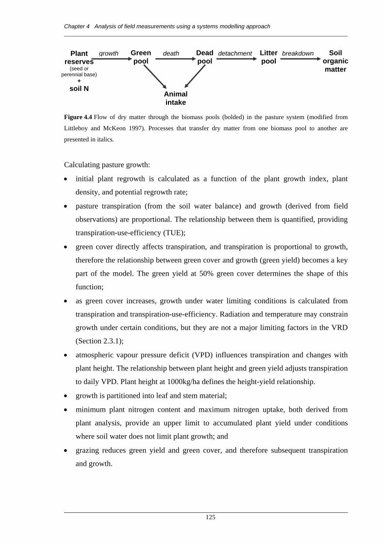
Chapter 4 Analysis of field measurements using a systems modelling approach
125
Figure 4.4 Flow of dry matter through the biomass pools (bolded) in the pasture system (modified from
Littleboy and McKeon 1997). Processes that transfer dry matter from one biomass pool to another are
presented in italics.
Calculating pasture growth:
• initial plant regrowth is calculated as a function of the plant growth index, plant
density, and potential regrowth rate;
• pasture transpiration (from the soil water balance) and growth (derived from field
observations) are proportional. The relationship between them is quantified, providing
transpiration-use-efficiency (TUE);
• green cover directly affects transpiration, and transpiration is proportional to growth,
therefore the relationship between green cover and growth (green yield) becomes a key
part of the model. The green yield at 50% green cover determines the shape of this
function;
• as green cover increases, growth under water limiting conditions is calculated from
transpiration and transpiration-use-efficiency. Radiation and temperature may constrain
growth under certain conditions, but they are not a major limiting factors in the VRD
(Section 2.3.1);
• atmospheric vapour pressure deficit (VPD) influences transpiration and changes with
plant height. The relationship between plant height and green yield adjusts transpiration
to daily VPD. Plant height at 1000kg/ha defines the height-yield relationship.
• growth is partitioned into leaf and stem material;
• minimum plant nitrogen content and maximum nitrogen uptake, both derived from
plant analysis, provide an upper limit to accumulated plant yield under conditions
where soil water does not limit plant growth; and
• grazing reduces green yield and green cover, and therefore subsequent transpiration
and growth.
Plant reserves
(seed or perennial base)
+ soil N
Green pool
death Dead pool
detachment Litter pool
breakdown
Animal intake
growth Soil organic matter

Chapter 4 Analysis of field measurements using a systems modelling approach
126
Plant death can occur in three ways: 1) a background death rate is applied, being directly
related to green yield; 2) an inverse relationship between soil water supply and plant death
is applied (plant death increases once soil water supply falls below a critical threshold);
and 3) frost may cause plant death, but this is not relevant to the VRD (Section 2.3.1).
Detachment of standing dead pasture due to wind and rain is calculated from a background
rate that is derived from field measurements. Mechanical detachment from disturbance by
grazing animals is also calculated, but pastures in this study were exclosed from grazing,
eliminating this form of detachment.
Breakdown of detached litter is determined from temperature and rainfall data, being
accelerated in warm, wet conditions (Robbins et al. 1989; Cooksley et al. 1993).
4.2.3 Assumptions and limitations of the model
A number of assumptions about the soil-plant-climate system are included in the GRASP
model. These assumptions are:
• for a given pasture type, there is no differentiation between species. All pasture is
treated as a green pool, dead pool, and litter pool;
• rainfall is the only source of soil water. There is no net run-on. Irrigation can be
incorporated but it is not applicable in this study;
• no use of water by grasses beyond a soil depth of 100cm, although the model can be
parameterised to access soil water below this depth;
• below-ground biomass accumulation (root growth) is not simulated, nor is seed
production;
• tree growth and senescence are not included;
• nutrients other than nitrogen are non-limiting;
• no reduction in nitrogen uptake occurs as a result of green material consumption by
grazing animals; and
• no impact on pasture growth by pests and disease.

Chapter 4 Analysis of field measurements using a systems modelling approach
127
4.3 Method for deriving model parameters and calibrating GRASP
The first major step in applying an empirically derived model such as GRASP to a new
situation is to calibrate the relationships it is built upon with local data (Figure 4.2). Rykiel
(1996) defines model calibration: “calibration is, in essence, the step of making a model as
consistent as possible with the data set from which the parameters are estimated”.
Calibration is often referred to as ‘model fitting’ as the process involves a certain amount
of parameter manipulation to produce the best fit between model output and the field
measured data. The calibration procedure in this study aims to provide sets of input
parameter values that best represent measured data for each site in each study year. This is
a variation from Day et al. (1997a) where a single set of parameters was established to
represent all years at a site. This approach was taken in order to maximise the number of
specific calibrated parameters available when deriving more generalised parameter sets
later in this thesis.
An optimisation technique such as least squares regression is often recommended for
calibration of model parameter values (e.g. Jones and Carberry 1994), but is not adopted
here. Optimisation has limitations as an appropriate technique for deriving parameters for
GRASP, due in part to the large number of parameters requiring simultaneous calibration.
Formal optimisation techniques may result in unrealistic parameter values even though
they produce acceptable results. This is expressed well by Carter et al. (1996b) who
suggest that it is possible at times to simulate the correct answer with incorrect parameters.
No formal algorithm yet exists to objectively calibrate GRASP from a measured dataset.
Consequently, the calibration procedure is manual and somewhat subjective. While the
procedure is essentially systematic, it does involve some judgement on:
• interpretation of the field results when making estimates of parameter values;
• specific parameters to target for individual site calibration;
• when ‘acceptable’ agreement between measured and modelled data is achieved; and
• deciding if individual field data points are atypical and excluding them from the
calibration procedure.
A large number of parameters in GRASP (100+) could potentially be calibrated. All
parameters have default values derived from field studies or literature. In practice, far

Chapter 4 Analysis of field measurements using a systems modelling approach
128
fewer than 100 parameters are actually calibrated for a given site. In this study 35
parameters were calibrated for each site, with the balance remaining at default values.
Individual calibrations of 21 sites over two years were undertaken, and in each case the
actual process was partially influenced by site characteristics. Hence, the exact calibration
procedure varied from site to site, but followed a general approach. An overview of this
approach to calibrating specific groups of parameters is provided to demonstrate how the
data presented in Chapter 3 was used to adapt the GRASP model to the grazing lands of
the VRD.
4.3.1 Input files
GRASP requires climate data from which to calculate the soil water balance and plant
growth, death and detachment processes. Spanning the two-year period of study at each
site, a climate file containing daily records of rainfall (measured at each of the study sites
or the nearest station homestead), pan evaporation, maximum and minimum temperature,
radiation, and vapour pressure (all from DataDrill 2005) defines the climatic environment
within which simulations will be made.
Model parameter values are specified in two separate input files. First, a file containing
initial (default) values for all parameters required for running GRASP has been developed
from previous studies. These parameters were established from the GUNSYNpD project
(McKeon et al. 1988; McKeon and Johnston 1990) and have been continually revised and
updated based upon subsequent studies and accumulating knowledge. Most parameters are
generally held at their default values. The default parameter file used in this study is shown
in Appendix 10.
A second file contains a number of more site-specific parameters that are either taken
directly, or derived, from field observations collected using the methodology of Day and
Philp (1997). As many parameters as possible are derived from the field data. These site-
specific parameter values overwrite the equivalent parameters in the default parameter file.
An example of a site-specific parameter file is shown in Appendix 10.

Chapter 4 Analysis of field measurements using a systems modelling approach
129
The following section details those parameters taken directly from field data, and those
parameters that used field data as an initial estimate and were then refined to provide a
better fit between the field dataset and model outputs. At first mention, individual model
parameters frequently referred to in the text are described in full with parameter names in
italics, followed by an abbreviation and a parameter reference number (e.g. p999).
Abbreviations are used thereafter.
4.3.2 Deriving individual parameter values
Soil water parameters
GRASP calculates the soil water balance for three layers: 1 (0 - 10cm), 2 (10 - 50cm) and 3
(50+cm). The depth of layers 1 and 2 (L1, p020 and L2, p021) are fixed, while the depth of
layer 3 (L3, p022) was determined from field data (pasture rooting depth e.g. Table 3.9).
Field capacity (FC) and Wilting point (WP) for each layer (p028 to p031) were also
sourced from field data presented in Section 3.4.2. Data collected on WP was considered
reliable but field measurements occasionally did not provide true FC (discussed in Section
3.5.1). Where model predictions of soil water did not coincide with field measurements,
adjustment to FC values was sometimes necessary to improve model performance. Runoff
of surface water (Runoff, p270) was allowed on red earths but not on cracking clays.
Calibrated values of soil parameters for all sites are presented in Table 4.1.
Parameters for soil layers 1 and 2 influence soil water in lower layers but parameters for
lower layers do not influence soil water in the layers above them; i.e. water only flows
downwards in GRASP. Cracking clays are often problematic to calibrate as moisture can
enter and leave the lower soil layers through the cracks without passing through the layers
above. Evaporation from cracks (Cracking, p035) is accounted for in GRASP, however
simultaneous wetting of the whole profile is not. Other soil types in the VRD do not crack.
Sward structure parameters
For much of the growing season, plant growth is related to transpiration. The relationships
between cover and yield, and height and yield, both influence transpiration and vary
considerably from pasture type to pasture type (Day et al. 1997a). Quantification of these
relationships for each study site requires specific values for Green plant yield at 50% green
cover (GY50GC, p045), and Plant height at 1000kg/ha (Ht1000kg, p096). Where field

Chapter 4 Analysis of field measurements using a systems modelling approach
130
measurements did not provide these values directly, they were estimated from regressions
of the data (e.g. Figure 3.22), and refined to optimise model performance. Calibrated
values of sward structure parameters for all sites are presented in Table 4.2.
Plant growth parameters
The Growth Index (Section 2.4) is the underlying principle governing plant growth in
GRASP and in the VRD soil water supply is the dominant component. However, other
factors are influential at different times during the growth cycle. Plant growth early in the
growing season depends upon plant density and regrowth from stored reserves. Perennial
grass basal area (PGBA, p005) was a direct field measurement of plant density (e.g. Table
3.17) and Potential regrowth rate per unit of PGBA (PotRegrow, p006) was estimated
from plant yield at the first harvest and the number of days elapsed since the initiation of
plant growth (Table 3.14).
After initial regrowth from stored reserves, the main phase of pasture growth is primarily
transpiration-dependent. Therefore, a key growth parameter in GRASP is Transpiration-
use-efficiency (TUE, p007). Preliminary estimates of TUE were derived from field data.
Estimates of evapotranspiration were calculated from rainfall received and changes in soil
water between one harvest and the next. Initial estimates of transpiration were set at 0.6
times evapotranspiration (K.A. Day pers. comm. based on extensive experience of
calibrating the model in Queensland, and supported by data in Murphy et al. 2004). Pasture
growth was estimated from changes in plant yield from one harvest to the next, with the
period between first and second harvests (H1 to H2 and H5 to H6, e.g. Figure 3.20 and
Table 9.12) being most important as growth is unlikely to be influenced by critical soil
water or nutrient limitations at this stage. Starting estimates of TUE were calculated from
pasture growth and transpiration values, and then refined during the calibration process to
provide better simulation results.
As the growing season concludes, soil water limitations reduce growth and senesce the
pasture. Values for the parameter Soil water index at which growth stops (SWIX0Grow,
p149) were held at default values unless model output showed poor correspondence with
field measurements. Soil water field data collected at the end of the growing season
provided a guide to refining these parameters for better model performance. Calibrated
values of plant growth parameters for all sites are presented in Table 4.3.

Chapter 4 Analysis of field measurements using a systems modelling approach
131
Nitrogen parameters
Nutrient supply (mainly nitrogen) is an important factor in pasture growth in the VRD
(Section 2.3.2). A number of parameters in GRASP specify the role of nitrogen, and values
for these come directly from field measurements. Examples of field data that provide these
parameter values are seen in Figure 3.21 and Table 3.16.
An internally stored supply of N initiates plant growth before root density is sufficient to
capture available N in the soil. The parameter N uptake at zero transpiration (Nup0Trans,
p097) represents this stored N supply and, along with Maximum N content in plant
material (Max%N, p100), was calculated from plant N analysis results at the first harvest
(e.g. Table 3.16).
Plant nitrogen status changes rapidly during the early growing season, and field
measurements did not always capture data that truly represents these parameters. This is
apparent in Figure 3.21 where the first harvest at Site 5 occurred in early February 1994,
some three months after growth began. Data recorded at this harvest did not provide
suitable values for Max%N (likely to have already peaked and declined), nor Nup0Trans
(uptake of N from soil already well under way). Consequently, values for these parameters
required refinement during the calibration procedure to provide better model predictions of
early season growth.
Other critical nitrogen parameters are also derived from plant analysis. At the end of the
growing season, values for Maximum N uptake (MaxN, p099), and N content at which
growth stops (%N0Grow, p101) and Minimum N content in dead plant material (Min%N,
p111) come directly from field data (e.g. Figure 3.24). Values for the parameter N uptake
per 100mm of transpiration (Nup100T, p098) is derived from field measurements of N
uptake throughout the growing season along with preliminary estimates of transpiration.
For field data to provide accurate values for these critical N parameters, plant growth
should not have ceased before they are fully expressed: i.e. drought conditions can senesce
plants before all available N is taken up by plants, or before they have internally diluted N
to their physiological limit. Seasonal conditions during the study period were generally
favourable and it is therefore assumed that field measurements provide suitable values for

Chapter 4 Analysis of field measurements using a systems modelling approach
132
the nitrogen parameters. Calibrated values of nitrogen parameters for all sites are presented
in Table 4.4.
Detachment parameters
Dead plant material detaches due to the action of wind and rain. The main period of
detachment is over the dry season. Differences in total plant yield between the end of the
growing season harvest, and end of the dry season harvest provide Detachment rate
parameter values (Detachment, p128 to p131). Calibrated values of detachment parameters
for all sites are presented in Table 4.6.
Tree parameters
Trees compete with pasture for soil water and nutrients. In this study, only one site
contained trees (Site 19). Tree basal area (TBA, p291) was estimated in the field, and Tree
wilting points (TWP) for the three soil layers (p292, p293 and p294) were set at the same
values as for the pasture. Table 4.5 contains tree basal area and tree wilting point values for
Site 19.
4.3.3 Summary
The first stage in calibrating GRASP for native pastures in the VRD is to derive a set of
initial parameter values based on local field data. Many parameter values are direct field
measurements (e.g. WP, PGBA, Max%N, Min%N and Detachment); others can be derived
from a series of field measurements (e.g. Ht1000kg, and GY50GC); and some parameters
(e.g. TUE) can only be calibrated by running the model with the best initial estimates of all
parameters, then refining their value to achieve more satisfactory simulation results.
The previous sections show how parameters that describe growth in GRASP have
influence at differing times throughout the growth cycle. Figure 4.5 illustrates typical daily
biomass accumulation simulated by GRASP for a native pasture in the VRD, and includes
parameters that are important at critical times.

Chapter 4 Analysis of field measurements using a systems modelling approach
133
Figure 4.5 Typical daily biomass accumulation curve for native pasture in the Victoria River District,
including approximate times of field measurements and the parameters in GRASP that are calibrated from
data collected at these times.
In a complex environment it is expected that discrepancies will occur between field
measured data and simulation model outputs. These discrepancies arise from deficiencies
in the model structure that do not account for the influence of some factors on site
processes, and measurement errors or omissions in data collection that set limits on the
accurate calibration of the model. In this study, the abbreviated ‘Swiftsynd’ methodology
(Day and Philp 1997) prescribes three measurement times during the growing season and
while every effort was made to coincide these measurements with critical times in the
pasture growth cycle, this was not always possible. Interpretation and judgement on those
situations where initial parameter values may need refinement requires an in-depth
understanding of the field data and the circumstances under which it was collected.
Reliable calibration is dependent on appropriate use and interpretation of field data, and
this is a major advantage of integrating the field experimental research with simulation
modelling, as undertaken in this study.
4.4 Results of calibration: Final model parameters
The parameter values established during the calibration process are specific to the
individual sites during the season of measurement. Many values will be the same or very
similar between years at the same site, but for some parameters (e.g. PotRegrow, TUE, and
0
1000
2000
3000
4000
Oct Jan Apr Jul Oct
Tota
l Sta
ndin
g D
ry M
atte
r (kg
/ha) Cumulative pasture biomass
Field measurements
Initial conditions described - soil water - total soil depth
First harvest - early wet season - max %N in plant - N uptake zero trans
Second harvest - mid wet season - soil water field capacity - grass basal area - cover vs yield relationship - height vs yield relationship
Third harvest - end of wet season - SWIX when growth stops - %N when growth stops - potential N uptake Fourth harvest - end of dry
season - soil water wilting point - leaf and stem detachment - min %N in plant

Chapter 4 Analysis of field measurements using a systems modelling approach
134
GY50GC) values can vary at the same site in different growing seasons. The final
calibrated parameter values for each site and each year are shown in Table 4.1 to Table 4.6
and these form the basis of all simulation studies in this thesis.
In a few instances during the calibration procedure, model predictions did not correspond
at all with field observations and special measures were required to improve the
simulations. These measures took two forms: 1) early growing season predictions of
TSDM were grossly under-predicted at Sites 9, 15 and 21 and the relationship between
green cover and green yield was reduced during this time to improve results (Table 4.2);
and 2) soil water values during December 1994 at Site 18 were much higher than predicted
and it was deduced that 100mm of surface run-on and/or unrecorded rainfall had occurred,
and the model was parameterised to account for this. Possible reasons for these difficulties
are discussed later in this chapter.
Finally, it is important to note that the final parameter calibration process is not completely
separate for each year at a site. Soil water parameter values (Table 4.1) are determined
from field measurements in both years and kept constant for all simulations at each site. In
a similar manner, some pasture growth parameters (i.e. TUE, PotRegrow, SWIX0Grow,
Table 4.3) and all nitrogen parameters (Table 4.4) are kept constant for both years at a site
unless conditions were so different between seasons that a change in value was necessary
to improve simulation results.

Chapter 4 Analysis of field measurements using a systems modelling approach
135
Table 4.1 Site-by-year calibrated GRASP soil parameters. (Table continued overleaf)
Parameter Pmtr No. S01Y11 S01Y2 S02Y1 S02Y2 S13Y1 S13Y2 S11Y1 S11Y2 S19Y1 S19Y2 S14Y1 S14Y2 S20Y1 S20Y2 Soil type REB2 REB REB REB REL REL REL REL REB REB REL REL ACC ACC Pasture type ASG3 ASG ASG ASG ASG ASG OPG OPG OPG OPG OPG OPG OPG OPG
Depth of layer 1 (mm) 020 100 100 100 100 100 100 100 100 100 100 100 100 100 100
Depth of layer 2 (mm) 021 400 400 400 400 400 400 400 400 400 400 400 400 400 400
Depth of layer 3 (mm) 022 500 500 500 500 0 0 100 100 500 500 100 100 500 500
Total depth of soil profile (mm) 1000 1000 1000 1000 500 500 600 600 1000 1000 600 600 1000 1000
Air dry layer 1 (mm) 019 3.5 3.5 3.5 3.5 3 3 3 3 4 4 2.5 2.5 5 5
Wilting point layer 1 (mm) 029 10 10 7 7 8 8 8 8 8 8 7 7 10 10
Field capacity layer 1 (mm) 026 35 35 35 35 35 35 33 33 35 35 25 25 35 35
Wilting point layer 2 (mm) 030 44 44 40 40 32 32 19 19 32 32 20 20 45 45
Field capacity layer 2 (mm) 027 130 130 120 120 130 130 65 65 120 120 110 110 130 130
Wilting point layer 3 (mm) 031 45 45 35 35 1 1 4.5 4.5 40 40 17 17 65 65
Field capacity layer 3 (mm) 028 130 130 115 115 2 2 16 16 120 120 35 35 150 150
Cracking (Yes/No) 035 No No No No No No No No No No No No Yes Yes
Runoff (Yes/No) 270 Yes Yes Yes Yes Yes Yes Yes Yes Yes Yes Yes Yes No No
WHC (fc-wp) layer 1 (mm) 25 25 28 28 27 27 25 25 27 27 18 18 25 25
WHC (fc-wp) layer 2 (mm) 86 86 80 80 98 98 46 46 88 88 90 90 85 85
WHC (fc-wp) layer 3 (mm) 85 85 80 80 1 1 11.5 11.5 80 80 18 18 85 85
WHC (fc-wp) layers 1-3 (mm) 196 196 188 188 126 126 82.5 82.5 195 195 126 126 195 195
WHC (fc-wp) average (mm/10cm) 19.6 19.6 18.8 18.8 25.2 25.2 13.8 13.8 19.5 19.5 21 21 19.5 19.5
1 S01Y1 is Site 1, Year 1; S01Y2 is Site 1, Year 2; and remaining headings follow this logic. Sites do not appear in numerical order across the table; instead, the order of
presentation is closely associated with soil type and species composition presented later in this thesis (Table 5.1 in Chapter 5). 2 REB is red earth overlying basalt; REL is red earth overlying limestone; CCB is cracking clay overlying basalt; and ACC is alluvial cracking clay. 3 ASG is annual short grasses; OPG is other perennial grasses; RG is ribbon grass; BMG is barley Mitchell grass; and F is forbs.

Chapter 4 Analysis of field measurements using a systems modelling approach
136
Table 4.1 (cont.) (Table continued overleaf)
Parameter Pmtr No. S12Y1 S12Y2 S08Y1 S08Y2 S10Y1 S10Y2 S16Y1 S16Y2 S07Y1 S07Y2 S09Y1 S09Y2 S21Y1 S21Y2 Soil type REL REL ACC ACC ACC ACC ACC ACC ACC ACC ACC ACC ACC ACC Pasture type OPG OPG RG RG RG RG RG RG RG RG RG RG F F
Depth of layer 1 (mm) 020 100 100 100 100 100 100 100 100 100 100 100 100 100 100
Depth of layer 2 (mm) 021 400 400 400 400 400 400 400 400 400 400 400 400 400 400
Depth of layer 3 (mm) 022 100 100 500 500 500 500 500 500 500 500 500 500 500 500
Total depth of soil profile (mm) 600 600 1000 1000 1000 1000 1000 1000 1000 1000 1000 1000 1000 1000
Air dry layer 1 (mm) 019 4 4 5 5 4 4 5 5 5 5 5 5 2.5 2.5
Wilting point layer 1 (mm) 029 7 7 12 12 10 10 10 10 12 12 12 12 7.5 7.5
Field capacity layer 1 (mm) 026 30 30 45 45 45 45 50 50 45 45 45 45 40 40
Wilting point layer 2 (mm) 030 60 60 50 50 45 45 50 50 45 45 50 50 25 25
Field capacity layer 2 (mm) 027 120 120 170 170 160 160 160 160 160 160 160 160 120 120
Wilting point layer 3 (mm) 031 13 13 80 80 60 60 70 70 90 90 80 80 50 50
Field capacity layer 3 (mm) 028 30 30 200 200 200 200 200 200 200 200 200 200 150 150
Cracking (Yes/No) 035 No No Yes Yes Yes Yes Yes Yes Yes Yes Yes Yes Yes Yes
Runoff (Yes/No) 270 Yes Yes No No No No No No No No No No No No
WHC (fc-wp) layer 1 (mm) 23 23 33 33 35 35 40 40 33 33 33 33 32.5 32.5
WHC (fc-wp) layer 2 (mm) 60 60 120 120 115 115 110 110 115 115 110 110 95 95
WHC (fc-wp) layer 3 (mm) 17 17 120 120 140 140 130 130 110 110 120 120 100 100
WHC (fc-wp) layers 1-3 (mm) 100 100 273 273 290 290 280 280 258 258 263 263 227.5 227.5
WHC (fc-wp) average (mm/10cm) 16.7 16.7 27.3 27.3 29 29 28 28 25.8 25.8 26.3 26.3 22.8 22.8

Chapter 4 Analysis of field measurements using a systems modelling approach
137
Table 4.1 (cont.)
Parameter Pmtr No. S04Y1 S04Y2 S15Y1 S15Y2 S05Y1 S05Y2 S03Y1 S03Y2 S18Y1 S18Y2 S06Y1 S06Y2 S17Y1 S17Y2 Soil type CCB CCB ACC ACC CCB CCB CCB CCB CCB CCB CCB CCB CCB CCB Pasture type F F F F BMG BMG BMG BMG BMG BMG BMG BMG OPG OPG
Depth of layer 1 (mm) 020 100 100 100 100 100 100 100 100 100 100 100 100 100 100
Depth of layer 2 (mm) 021 400 400 400 400 400 400 400 400 400 400 400 400 400 400
Depth of layer 3 (mm) 022 400 400 500 500 500 500 500 500 300 300 200 200 400 400
Total depth of soil profile (mm) 900 900 1000 1000 1000 1000 1000 1000 800 800 700 700 900 900
Air dry layer 1 (mm) 019 5 5 4 4 5 5 5 5 5 5 4 4 4 4
Wilting point layer 1 (mm) 029 10 10 10 10 10 10 10 10 10 10 10 10 10 10
Field capacity layer 1 (mm) 026 45 45 45 45 50 50 45 45 50 50 45 45 50 50
Wilting point layer 2 (mm) 030 40 40 40 40 40 40 50 50 50 50 40 40 40 40
Field capacity layer 2 (mm) 027 160 160 160 160 200 200 190 190 190 190 180 180 160 160
Wilting point layer 3 (mm) 031 60 60 80 80 100 100 100 100 60 60 25 25 60 60
Field capacity layer 3 (mm) 028 180 180 200 200 250 250 250 250 150 150 95 95 180 180
Cracking (Yes/No) 035 Yes Yes Yes Yes Yes Yes Yes Yes Yes Yes Yes Yes Yes Yes
Runoff (Yes/No) 270 No No No No No No No No No No No No No No
WHC (fc-wp) layer 1 (mm) 35 35 35 35 40 40 35 35 40 40 35 35 40 40
WHC (fc-wp) layer 2 (mm) 120 120 120 120 160 160 140 140 140 140 140 140 120 120
WHC (fc-wp) layer 3 (mm) 120 120 120 120 150 150 150 150 90 90 70 70 120 120
WHC (fc-wp) layers 1-3 (mm) 275 275 275 275 350 350 325 325 270 270 245 245 280 280
WHC (fc-wp) average (mm/10cm) 30.6 30.6 27.5 27.5 35 35 32.5 32.5 33.8 33.8 35 35 31.1 31.1

Chapter 4 Analysis of field measurements using a systems modelling approach
138
Table 4.2 Site-by-year calibrated GRASP sward structure parameters. (Table continued below)
Parameter Pmtr No. S01Y1 S01Y2 S02Y1 S02Y2 S13Y1 S13Y2 S11Y1 S11Y2 S19Y1 S19Y2 S14Y1 S14Y2 S20Y1 S20Y2 Soil type REB REB REB REB REL REL REL REL REB REB REL REL ACC ACC Pasture type ASG ASG ASG ASG ASG ASG OPG OPG OPG OPG OPG OPG OPG OPG Green standing dry matter at 50% green
cover for calculation of transpiration,
radiation interception and runoff (kg/ha)
045, 046 and
271 700 1500 500 1600 800 1500 1800 1650 1450 2050 1900 2550 1050 1600
Height of 1000kg/ha TSDM (cm) 096 10 10 12 10 11 15 10 13 16 24 13 22 16 14
Table 4.2 (cont.) (Table continued below)
Parameter Pmtr No. S12Y1 S12Y2 S08Y1 S08Y2 S10Y1 S10Y2 S16Y1 S16Y2 S07Y1 S07Y2 S09Y1 S09Y2 S21Y1 S21Y2 Soil type REL REL ACC ACC ACC ACC ACC ACC ACC ACC ACC ACC ACC ACC Pasture type OPG OPG RG RG RG RG RG RG RG RG RG RG F F Green standing dry matter at 50% green
cover for calculation of transpiration,
radiation interception and runoff (kg/ha)
045, 046 and
271 1800 1750 1500 1300 1650 1650 1450 1700 1200 1450 1550 1750 1350 1200
Until 1st harvest change yield at 50% cover
to this value (kg/ha) 500 500
Height of 1000kg/ha TSDM (cm) 096 15 13 10 14 12 11 11 13 8 12 14 11 13 10
Table 4.2 (cont.)
Parameter Pmtr No. S04Y1 S04Y2 S15Y1 S15Y2 S05Y1 S05Y2 S03Y1 S03Y2 S18Y1 S18Y2 S06Y1 S06Y2 S17Y1 S17Y2 Soil type CCB CCB ACC ACC CCB CCB CCB CCB CCB CCB CCB CCB CCB CCB Pasture type F F F F BMG BMG BMG BMG BMG BMG BMG BMG OPG OPG Green standing dry matter at 50% green
cover for calculation of transpiration,
radiation interception and runoff (kg/ha)
045, 046 and
271 850 850 1650 1450 2300 1650 2050 1600 1100 1650 1600 1400 1900 2200
Until 1st harvest change yield at 50% cover
to this value (kg/ha) 500
Height of 1000kg/ha TSDM (cm) 096 8 8 8 10 10 11 15 11 17 14 8 14 14 15

Chapter 4 Analysis of field measurements using a systems modelling approach
139
Table 4.3 Site-by-year calibrated GRASP plant growth parameters. (Table continued below)
Parameter Pmtr No. S01Y1 S01Y2 S02Y1 S02Y2 S13Y1 S13Y2 S11Y1 S11Y2 S19Y1 S19Y2 S14Y1 S14Y2 S20Y1 S20Y2 Soil type REB REB REB REB REL REL REL REL REB REB REL REL ACC ACC Pasture type ASG ASG ASG ASG ASG ASG OPG OPG OPG OPG OPG OPG OPG OPG
Perennial grass basal area (%) 005 8.4 1.63 6 0.38 5.75 0.38 2.88 2.75 1.88 0.63 2.88 2.13 0.88 2
Potential regrowth rate / unit PGBA
(kg/ha/day/basal%) 006 3 8 2 34.2 2.5 13 8 8 9 9 4 4 10 10
Transpiration-use-efficiency (kg/ha/mmT) 007 8 13.5 9 13.5 9 9 15 8 10 9 12 10 12 12
Soil water index at which growth stops 149 0.01 0.01 0.01 0.01 0.01 0.01 0.3 0.3 0.3 0.3 0.3 0.3 0.3 0.3
Table 4.3 (cont.) (Table continued below)
Parameter Pmtr No. S12Y1 S12Y2 S08Y1 S08Y2 S10Y1 S10Y2 S16Y1 S16Y2 S07Y1 S07Y2 S09Y1 S09Y2 S21Y1 S21Y2 Soil type REL REL ACC ACC ACC ACC ACC ACC ACC ACC ACC ACC ACC ACC Pasture type OPG OPG RG RG RG RG RG RG RG RG RG RG F F
Perennial grass basal area (%) 005 1.25 2.13 6 4.25 4.25 3.5 1.63 1.5 2.25 3.25 0.88 2.13 3.25 1.63
Potential regrowth rate / unit PGBA
(kg/ha/day/basal%) 006 15 10 6 6 6 6 10 6 9 9 8 8 6 6
Transpiration-use-efficiency (kg/ha/mmT) 007 13 10 9 9 9 9 16 9 8 8 14 14 8 10
Soil water index at which growth stops 149 0.3 0.3 0.3 0.3 0.3 0.3 0.3 0.3 0.3 0.3 0.3 0.3 0.3 0.3
Table 4.3 (cont.)
Parameter Pmtr No. S04Y1 S04Y2 S15Y1 S15Y2 S05Y1 S05Y2 S03Y1 S03Y2 S18Y1 S18Y2 S06Y1 S06Y2 S17Y1 S17Y2 Soil type CCB CCB ACC ACC CCB CCB CCB CCB CCB CCB CCB CCB CCB CCB Pasture type F F F F BMG BMG BMG BMG BMG BMG BMG BMG OPG OPG
Perennial grass basal area (%) 005 1 1 0.75 1.5 3.63 3.75 4.5 3.75 2.38 2.13 1.5 1.3 3 1.33
Potential regrowth rate / unit PGBA
(kg/ha/day/basal%) 006 14 14 10 10 8 8 5 5 10 10 10 10 10 12
Transpiration-use-efficiency (kg/ha/mmT) 007 16 16 10 10 10 10 8 8 10 10 16 16 10 10
Soil water index at which growth stops 149 0.01 0.01 0.01 0.01 0.01 0.01 0.01 0.01 0.01 0.01 0.01 0.01 0.01 0.01

Chapter 4 Analysis of field measurements using a systems modelling approach
140
Table 4.4 Site-by-year calibrated GRASP nitrogen parameters. (Table continued below)
Parameter Pmtr No. S01Y1 S01Y2 S02Y1 S02Y2 S13Y1 S13Y2 S11Y1 S11Y2 S19Y1 S19Y2 S14Y1 S14Y2 S20Y1 S20Y2 Soil type REB REB REB REB REL REL REL REL REB REB REL REL ACC ACC Pasture type ASG ASG ASG ASG ASG ASG OPG OPG OPG OPG OPG OPG OPG OPG
N uptake at 0 mm of transpiration (kg/ha) 097 4.0 4.0 2.0 2.0 1.0 1.0 7.0 7.0 2.0 3.0 1.0 1.0 2.0 2.0
N uptake per 100mm of transpiration
(kg/ha/100mmT) 098 10 10 10 10 8 8 10 10 8 8 7 7 8 8
Maximum nitrogen uptake (kg/ha) 099 21 25 24 20 18 10 18 18 10 10 13 13 19 19
Maximum nitrogen content in plants (%) 100 2.5 3.5 2.5 3.5 2.5 2.5 2.5 2.5 2.5 2.5 2.5 2.5 2.5 2.5
N content at which growth stops (%) 101 0.8 0.8 0.8 0.8 0.65 0.65 0.65 0.7 0.5 0.5 0.45 0.45 0.7 0.45
N content at which growth is restricted (%) 102 0.9 0.9 0.9 0.9 0.75 0.75 0.75 0.8 0.6 0.6 0.55 0.55 0.8 0.55
Minimum N content in dead (%) 111 0.8 0.9 0.9 0.8 0.7 0.7 0.4 0.5 0.5 0.9 0.4 0.6 0.4 0.3
Table 4.4 (cont.) (Table continued overleaf)
Parameter Pmtr No. S12Y1 S12Y2 S08Y1 S08Y2 S10Y1 S10Y2 S16Y1 S16Y2 S07Y1 S07Y2 S09Y1 S09Y2 S21Y1 S21Y2 Soil type REL REL ACC ACC ACC ACC ACC ACC ACC ACC ACC ACC ACC ACC Pasture type OPG OPG RG RG RG RG RG RG RG RG RG RG F F
N uptake at 0 mm of transpiration (kg/ha) 097 1.0 1.0 4.0 4.0 3.0 3.0 5.0 8.0 5.0 5.0 5.0 7.0 1.0 5.0
N uptake per 100mm of transpiration
(kg/ha/100mmT) 098 14 14 7 7 10 10 14 6 14 14 10 10 8 8
Maximum nitrogen uptake (kg/ha) 099 21 21 21 37 21 21 29 23 28 28 17 23 19 19
Maximum nitrogen content in plants (%) 100 2.5 2.5 2.5 2.5 2.5 2.5 2.5 2.5 2.5 2.5 2.5 2.5 2.5 2.5
N content at which growth stops (%) 101 0.7 0.7 0.6 0.6 0.7 0.7 0.9 0.8 0.7 0.7 0.85 0.85 0.9 1.1
N content at which growth is restricted (%) 102 0.8 0.8 0.7 0.7 0.8 0.8 1 0.9 0.8 0.8 0.95 0.95 1 1.2
Minimum N content in dead (%) 111 0.5 0.7 0.4 0.4 0.4 0.4 0.5 0.8 0.5 0.6 0.5 0.5 0.5 0.9

Chapter 4 Analysis of field measurements using a systems modelling approach
141
Table 4.4 (cont.)
Parameter Pmtr No. S04Y1 S04Y2 S15Y1 S15Y2 S05Y1 S05Y2 S03Y1 S03Y2 S18Y1 S18Y2 S06Y1 S06Y2 S17Y1 S17Y2 Soil type CCB CCB ACC ACC CCB CCB CCB CCB CCB CCB CCB CCB CCB CCB Pasture type F F F F BMG BMG BMG BMG BMG BMG BMG BMG OPG OPG
N uptake at 0 mm of transpiration (kg/ha) 097 2.0 2.0 10.0 10.0 7.0 1.0 1.0 1.0 5.0 5.0 1.0 1.0 1.0 1.0
N uptake per 100mm of transpiration
(kg/ha/100mmT) 098 14 14 12 12 10 10 9 9 10 10 16 16 14 18
Maximum nitrogen uptake (kg/ha) 099 36 36 38 38 35 35 29 29 21 15 27 27 15 15
Maximum nitrogen content in plants (%) 100 2.5 2.5 2.5 2.5 2.5 2.5 2.5 2.5 2.5 2.5 3.5 3.5 2.5 2.5
N content at which growth stops (%) 101 1.2 1.2 1.35 1.2 0.65 0.65 0.5 0.5 0.6 0.6 0.8 0.8 0.6 0.8
N content at which growth is restricted (%) 102 1.3 1.3 1.45 1.3 0.75 0.75 0.6 0.6 0.7 0.7 0.9 0.9 0.7 0.9
Minimum N content in dead (%) 111 0.9 0.9 0.7 0.7 0.5 0.5 0.5 0.5 0.4 0.4 0.5 0.5 0.4 0.6
Table 4.5 Tree parameters for Site 19.
Parameter Pmtr No. S19Y1 S19Y2 Soil type REB REB Pasture type OPG OPG
Tree Basal Area (m2) 291 0.9 0.9
Wilting point layer 1 for trees 292 4 4
Wilting point layer 2 for trees 293 32 32
Wilting point layer 3 for trees 294 40 40
Note: No other sites contained trees.

Chapter 4 Analysis of field measurements using a systems modelling approach
142
Table 4.6 Site-by-year calibrated GRASP detachment parameters. (Table continued below)
Parameter Pmtr No. S01Y1 S01Y2 S02Y1 S02Y2 S13Y1 S13Y2 S11Y1 S11Y2 S19Y1 S19Y2 S14Y1 S14Y2 S20Y1 S20Y2 Soil type REB REB REB REB REL REL REL REL REB REB REL REL ACC ACC Pasture type ASG ASG ASG ASG ASG ASG OPG OPG OPG OPG OPG OPG OPG OPG
Leaf detachment - wet season (kg/kg/day) 128 0.0005 0.002 0.001 0.003 0.0015 0.005 0.0005 0.0005 0.003 0.003 0.0025 0.0005 0.0015 0.0015
Stem detachment - wet season (kg/kg/day) 129 0.0005 0.002 0.001 0.003 0.0015 0.005 0.0005 0.0005 0.003 0.003 0.0025 0.0005 0.0015 0.0015
Leaf detachment - dry season (kg/kg/day) 130 0.0005 0.002 0.001 0.003 0.0015 0.005 0.0005 0.0005 0.003 0.003 0.0025 0.0005 0.0015 0.0015
Stem detachment - dry season (kg/kg/day) 131 0.0005 0.002 0.001 0.003 0.0015 0.005 0.0005 0.0005 0.003 0.003 0.0025 0.0005 0.0015 0.0015
Table 4.6 (cont.) (Table continued below)
Parameter Pmtr No. S12Y1 S12Y2 S08Y1 S08Y2 S10Y1 S10Y2 S16Y1 S16Y2 S07Y1 S07Y2 S09Y1 S09Y2 S21Y1 S21Y2 Soil type REL REL ACC ACC ACC ACC ACC ACC ACC ACC ACC ACC ACC ACC Pasture type OPG OPG RG RG RG RG RG RG RG RG RG RG F F
Leaf detachment - wet season (kg/kg/day) 128 0.0005 0.001 0.0015 0.003 0.004 0.004 0.003 0.003 0.001 0.0035 0.001 0.004 0.003 0.003
Stem detachment - wet season (kg/kg/day) 129 0.0005 0.001 0.0015 0.003 0.004 0.004 0.003 0.003 0.001 0.0035 0.001 0.004 0.003 0.003
Leaf detachment - dry season (kg/kg/day) 130 0.0005 0.001 0.0015 0.003 0.004 0.004 0.003 0.003 0.001 0.0035 0.001 0.004 0.003 0.003
Stem detachment - dry season (kg/kg/day) 131 0.0005 0.001 0.0015 0.003 0.004 0.004 0.003 0.003 0.001 0.0035 0.001 0.004 0.003 0.003
Table 4.6 (cont.)
Parameter Pmtr No. S04Y1 S04Y2 S15Y1 S15Y2 S05Y1 S05Y2 S03Y1 S03Y2 S18Y1 S18Y2 S06Y1 S06Y2 S17Y1 S17Y2 Soil type CCB CCB ACC ACC CCB CCB CCB CCB CCB CCB CCB CCB CCB CCB Pasture type F F F F BMG BMG BMG BMG BMG BMG BMG BMG OPG OPG
Leaf detachment - wet season (kg/kg/day) 128 0.005 0.003 0.002 0.005 0 0.0025 0.0002 0.004 0.001 0.002 0.001 0.001 0.0035 0.003
Stem detachment - wet season (kg/kg/day) 129 0.005 0.003 0.002 0.005 0 0.0025 0.0002 0.004 0.001 0.002 0.001 0.001 0.0035 0.003
Leaf detachment - dry season (kg/kg/day) 130 0.005 0.003 0.002 0.005 0 0.0025 0.0002 0.004 0.001 0.002 0.001 0.001 0.0035 0.003
Stem detachment - dry season (kg/kg/day) 131 0.005 0.003 0.002 0.005 0 0.0025 0.0002 0.004 0.001 0.002 0.001 0.001 0.0035 0.003

Chapter 4 Analysis of field measurements using a systems modelling approach
143
4.5 Comparing model outputs with field data
The calibration process includes comparison of model outputs of important variables with
the field measurements reported in Chapter 3. Four main variables were compared:
• plant available soil water content (PAWC, from MLA 2004a), the amount of soil water
above wilting point and therefore available for transpiration and plant growth;
• green cover (Cover), the proportion of the ground surface covered by transpiring green
plant material;
• nitrogen uptake (N uptake), the total amount of nitrogen the pasture plant contains; and
• total standing dry matter (TSDM), the net result of pasture growth, death and
detachment (largely dependent on the three previous variables).
Three measures of comparing the level of agreement between model outputs and field
measurements are used to evaluate model performance in this section.
Literature relevant to this study uses specific terms relating to the comparison of modelling
outputs and field measured data. Modelling outputs, or simulation results, are expressed as
‘predictions’ as the intention of models like GRASP is to extrapolate variables such as
TSDM beyond field measurements. Field-measured data are commonly expressed as
‘observations’. These terms are applied accordingly throughout this thesis.
4.5.1 Methods
Time-series plots
Mayer and Butler (1993) and Rykiel (1996) recognise visual techniques as one means of
assessing model performance. Time-series plots of predictions and observations of
important variables form the basis of comparisons between model and real system. This
method of assessing the adequacy of calibration parameters is a useful tool for gaining an
initial view of how well the real system is being replicated.
Time series data, while visually informative for individual sites, do not provide objective
evaluation of the overall performance of the model. Two statistical approaches are used for
more meaningful analysis of simulation results: 1) regression analysis; and 2) measures of
prediction deviance. These approaches are explained and applied below.

Chapter 4 Analysis of field measurements using a systems modelling approach
144
Regression analysis
The statistical correlation between predicted and observed data is a common objective
measure of model performance during calibration (Jones and Carberry 1994; Rykiel 1996;
Grant et al. 1997). Mayer et al. (1994) list key assumptions for using regression statistics
to test model performance, including that all points within a dataset are independent of
each other. Time-series data, like those in this study, are auto-correlated and therefore not
independent; i.e. TSDM at time 2 (e.g. end of wet season) is dependent on TSDM at time 1
(e.g. mid wet season), as well as growth and detachment between time 1 and time 2.
Observations made at different sites or in different seasons are, however, statistically
independent of each other. Thus, by using subsets consisting of data points from different
sites at the same time of the growing season, and from the same site and time but in
different growing seasons, datasets of ‘independent’ points can be constructed and
subjected to statistical analysis. The four subsets of independent data in this study are
‘Early wet’ (data from Harvest 1 and Harvest 5 at all sites), ‘Mid wet’ (Harvest 2 and 6),
‘End of wet’ (Harvest 3 and 7), and ‘End of dry’ (Harvest 4 and 8).
Measuring model performance using regression statistics often involves assessing
predictions against the ‘perfect fit’ function of unity slope and zero intercept (y = x, or the
one-is-to-one line, Mayer et al. 1994; Asseng et al. 1998). As data points are compared to a
set function and not the line of best fit, values for the one-is-to-one statistic are usually
lower than for the more widely used coefficient of determination (r2) if calculated from the
same dataset. The GRASP model has been tested previously using the one-is-to-one
statistic (McKeon et al. 1990; Johnston 1996; Day et al. 1997a; Dyer et al. 2001a). While
many studies report results using this statistic, few provide details of its calculation. In this
study, the one-is-to-one statistic is calculated according to Mayer and Butler (1993), who
define it as ‘modelling efficiency’ (EF):
EF = 1 - (SS about y = x) / (Corrected SS of y)
= 1 - Σ(yi – xi)2 / Σ(yi – mean of y)2 (Equation 9)
where SS is the sum of squares, yi are observed values and xi are corresponding predicted
values.

Chapter 4 Analysis of field measurements using a systems modelling approach
145
Mayer and Butler (1993) explain the interpretation of EF: “r2 is interpreted as the
proportion of variation explained by the fitted regression line, and EF is a similar measure
against the set line y = x. For regression, the line of best fit cannot be worse than y = mean
of x, so r2 has a lower bound of zero. In Equation 9 the data are compared with a fixed
line, so this restriction is removed. Thus, EF has a (theoretical) lower bound of negative
infinity. A value of zero indicates the fit to y = x is equal to the fit to y = mean of x, with
values of EF less than zero resulting in a worse fit. The calculated EF is thus an overall
indication of goodness of fit. Any model giving a negative value cannot be recommended,
with preferable values close to one indicating a ‘near-perfect’ model.” In this thesis, EF is
referred to by the more common label, r2(1:1).
Prediction variance: Root Mean Squared Error
Another common measure of model performance is based on the actual differences
between observed values and the associated model predictions. Wallach and Goffinet
(1989) and Jones and Carberry (1995) use prediction variance, or the mean squared error
of prediction (MSEP) to measure model performance. Mayer and Butler (1993) present the
related value, root mean squared error (RMSE), sometimes called root mean squared
deviation or difference (RMSD), and GRASP has previously been assessed using this
statistic (Day et al. 1993). RMSE is a useful measure of model performance as it “indicates
the relative degree of model deviation from field observations, and can be used to
determine further statistical properties” (Mayer and Butler 1993).
Mayer and Butler (1993) define RMSE as:
RMSE = {(Σ(yi – xi)2) / n}0.5 (Equation 10)
where yi are observed values, xi are corresponding predicted values, and n is the number of
data pairs.
The higher the value for RMSE, the greater the overall difference between model
predictions and field observations. Relative prediction error can be determined from

Chapter 4 Analysis of field measurements using a systems modelling approach
146
comparing RMSE to the mean of observed data. These values have been calculated for the
four main variables and are presented in Table 4.7.
Prediction variance: Deviation of predictions from observed data
Mitchell and Sheehy (1997) present an alternative measure of model performance based
upon deviation of predictions from their associated observation values. These deviations
are analogous to the ‘error’ in RMSE. This method plots deviations (as prediction minus
observation) against the observations. The two criteria used to assess model performance
are the ‘envelope’ of acceptable precision about the line of zero deviation, and the
proportion of points that lie within it. Instances where the prediction values are less than
the envelope of acceptable precision are considered under-predictions. Over-prediction
occurs when the predictions exceed the envelope. Model performance can be assessed for
individual growth phases, and across the whole growth cycle using this method.
Rykiel (1996) suggests measurement variance (e.g. 95% confidence limits of the observed
data) as criteria for acceptable model precision. The method of field data collection in this
study has restricted calculation of reliable measurement variance to TSDM data. (Table
9.12 in Appendix 7). Therefore, assessing model performance using the deviations method
is only possible for predictions of TSDM. Two approaches to using measurement variance
as the envelope of acceptable precision have been adopted in this study:
• Each prediction was compared to the individual 95% confidence limits of the
corresponding observation to determine whether it was inside or outside the limits; and
• Each prediction was also compared to the average 95% confidence limits for all
observations (that is, ±35% of the observation value - Table 3.34 in Section 3.5.3) to
determine whether it was inside or outside the limits.
Where predictions fall within the confidence limits, they are considered as reliable an
estimate of TSDM as actually measuring this variable in the field using the methodology
applied in this study.

Chapter 4 Analysis of field measurements using a systems modelling approach
147
4.5.2 Results
Time-series plots
Figure 4.6 shows time-series plots of TSDM, N uptake, PAWC and Cover for several sites
with differing soil types and species compositions as examples of this method of
comparison. Model predictions are presented as a continuous line and field observations
are displayed as isolated points. The TSDM plots also include 95% confidence limits for
the observation values, and where the prediction line passes within these limits the
prediction is not significantly different to the observation.
Both TSDM time-series plots in Figure 4.6 display close visual agreement between
predictions and observations, except for points early in each growing season at Site 4.
Overall, the time-series plots of TSDM resulting from all individual site and year
simulations were similar in appearance to the two presented here, with observations and
predictions generally corresponding except for a few individual points.
Model predictions of PAWC also show close agreement with observations, with departures
of model predictions from the measured data apparent in some instances. The two
examples of PAWC time-series illustrated in Figure 4.6 represent a very high water
holding capacity soil (Site 5) and a very low water holding capacity soil (Site 12), and the
good visual results suggest GRASP can adequately simulate water balances across a range
of soil types in the region when using local parameter sets.
N uptake and Cover show the most discrepancies between predictions and observations in
the examples presented here. The N uptake predictions for Site 1 clearly correspond with
measured data and demonstrate how well GRASP can simulate this variable. Alternatively,
predictions of N uptake at Site 14 deviate considerably from the measured data and are an
example of poor model performance. Green plant cover also proved difficult to simulate
and some predictions are inconsistent with the field measurements. This has implications
for the calculations of the water balance and plant growth as green cover is an important
variable in calculating evaporation and transpiration, and hence pasture growth. These
implications are discussed later in this chapter.

Chapter 4 Analysis of field measurements using a systems modelling approach
148
Figure 4.6 Examples of time-series plots of prediction curves (lines) with observed values (points, including
95% confidence limits in the TSDM plots). Data presented are from sites of different soil type and pasture
species composition: Site 4 (forbs on basalt clay); Site 8 (ribbon grass on alluvial clay); Site 1 (annual short
grasses on basalt red earth); Site 14 (other perennial grasses on limestone red earth); Site 5 (barley Mitchell
grass on basalt clay); Site 12 (other perennial grasses on limestone red earth); Site 3 (barley Mitchell grass on
basalt clay); and Site 15 (forbs on alluvial clay).
Site 4
0
1000
2000
3000
4000
5000
Jul-93 Jan-94 Jul-94 Jan-95 Jul-95
Tota
l sta
ndin
g dr
y m
atte
r (kg
/ha)
Observed
PredictedSite 8
0
1000
2000
3000
4000
5000
Jul-93 Jan-94 Jul-94 Jan-95 Jul-95
Tota
l sta
ndin
g dr
y m
atte
r (kg
/ha)
Observed
Predicted
Site 1
0
5
10
15
20
25
30
Jul-93 Jan-94 Jul-94 Jan-95 Jul-95
Nitr
ogen
upt
ake
(kg/
ha)
Observed
PredictedSite 14
0
5
10
15
20
25
30
Jul-94 Jan-95 Jul-95 Jan-96 Jul-96
Nitr
ogen
upt
ake
(kg/
ha)
Observed
Predicted
Site 5
0
100
200
300
400
Jul-93 Jan-94 Jul-94 Jan-95 Jul-95
Plan
t ava
ilabl
e w
ater
con
tent
(mm
) Observed
PredictedSite 12
0
100
200
300
400
Jul-93 Jan-94 Jul-94 Jan-95 Jul-95
Plan
t ava
ilabl
e w
ater
con
tent
(mm
) Observed
Predicted
Site 3
0
20
40
60
80
100
Jul-93 Jan-94 Jul-94 Jan-95 Jul-95
Gre
en p
lant
cov
er (%
)
Observed
PredictedSite 15
0
20
40
60
80
100
Jul-94 Jan-95 Jul-95 Jan-96 Jul-96
Gre
en p
lant
cov
er (%
)
Observed
Predicted

Chapter 4 Analysis of field measurements using a systems modelling approach
149
Regression statistics
Figure 4.7 displays predictions against observations as a measure of assessing the overall
performance of the final calibration parameters for all individual sites. Four variables
presented are presented: TSDM, N Uptake, PAWC, and Cover. PAWC is presented as
plant available soil water content per 50cm of soil depth. Sites differ in their total soil
profile depth, but the 0 - 50cm soil depth is common to all sites and is the most important
for pasture growth (Christie 1981). Consequently, data for this profile depth are presented
to maintain consistency across sites.
In Figure 4.7, the predicted values are plotted on the x-axis and the observed values on the
y-axis. This format has been adopted according to Mayer and Butler (1993), who reason
that “to conform with statistical assumptions, it is usual to take the observations as the Y-
variate (as these data contain natural variability) and the model predictions as the non-
variable X’s”. The statistical assumptions they refer to are that errors on dependent
variables (field observations) are normally and independently distributed, and that
independent variables are without error (i.e. model predictions are single values and have
no statistical error).
The TSDM plot in Figure 4.7 displays a good overall fit between model predictions and
field observations, particularly at the end of the wet season and end of the dry season
where predictions lie very close to the 1:1 line. Statistics in Table 4.7 confirm that GRASP
simulated this variable with great accuracy at these times (r2(1:1) = 0.966 and 0.954
respectively). Some individual prediction errors are evident, particularly early in the wet
season when a number of over-predictions of TSDM occur, reducing model performance at
this time (r2(1:1) = 0.588).
Figure 4.7 also appears to show good model performance for prediction of PAWC in many
instances. Closer inspection, however, reveals a wide scatter of points at values of less than
100mm/50cm. These soil water contents mostly occurred at the beginning and end of the
growing season and regression statistics confirm that model performance was poorest at
these times (r2(1:1) = 0.510 for the early wet and r2(1:1) = 0.280 for the end of the wet -
Table 4.7). Importantly, during the mid wet season when plant water use is high and
pasture growth rapid, predictions of PAWC were accurate (r2(1:1) = 0.874). The low water
contents at the end of the dry season were also closely predicted (r2(1:1) = 0.926).

Chapter 4 Analysis of field measurements using a systems modelling approach
150
Predictions of N uptake in Figure 4.7 show greater spread about the 1:1 line than do
predictions of the previous two variables, but many points still lie close to the line,
indicating fair overall model performance. End of wet season N uptake is well simulated
by GRASP (r2(1:1) = 0.774). Early wet season and mid wet season predictions showed
greater variability (r2(1:1) = 0.417 and 0.518 respectively), while end of dry season
predictions of N uptake contained many errors and had no relationship with the observed
data (r2(1:1) = -4.460).
Predictions of green plant cover did not correspond well with observations. Many large
predictions errors occurred in the early wet season (r2(1:1) = 0.284), and almost total over-
prediction of mid wet season cover is an obvious feature of Figure 4.7 (r2(1:1) = -0.576).
End of wet season and end of dry season cover predictions show little agreement with
observed data (r2(1:1) = -0.026 and r2(1:1) = -1.208 respectively).

Chapter 4 Analysis of field measurements using a systems modelling approach
151
Figure 4.7 Observed vs. predicted data for all sites. Model predictions are the results of using individual site
parameter sets. Variables presented are total standing dry matter (TSDM), nitrogen uptake (N uptake), plant
available water content in the 0-50cm layer of the soil (PAWC), and green plant cover. Associated statistics
are presented in Table 4.7.
Prediction variance: Root Mean Squared Error
RMSE values presented here have been calculated from the same dataset as presented in
Figure 4.7 and are used in conjunction with the regression statistics to build a picture of
model performance.
Calculation of RMSE for predictions of TSDM produced relatively high error values for
the early and mid wet season (RMSE = 273 and 363 kg/ha respectively), and much lower
values at the end of the wet and end of the dry season (RMSE = 132 and 129kg/ha)
0
1000
2000
3000
4000
5000
0 1000 2000 3000 4000 5000
Predicted TSDM (kg/ha)
Obs
erve
d TS
DM
(kg/
ha)
Early wetMid wetEnd of wetEnd of dry
1:1n=163
0
10
20
30
40
50
0 10 20 30 40 50
Predicted N uptake (kg/ha)
Obs
erve
d N
upt
ake
(kg/
ha)
Early wetMid wetEnd of wetEnd of dry
1:1n=163
0
50
100
150
200
250
300
0 50 100 150 200 250 300
Predicted PAWC (mm/50cm)
Obs
erve
d PA
WC
(mm
/50c
m)
Early wetMid wetEnd of wetEnd of dry
n=162 1:1
0
20
40
60
80
100
0 20 40 60 80 100
Predicted green cover (%)
Obs
erve
d gr
een
cove
r (%
)
Early wetMid wetEnd of wetEnd of dry
n=163 1:1

Chapter 4 Analysis of field measurements using a systems modelling approach
152
indicating better model performance at these times. Results of RMSE showed the same
trends in model performance for TSDM as did the regression statistics.
Results for mid wet season and end of wet season predictions of PAWC have an interesting
feature. Using RMSE alone as an indicator of model performance suggests GRASP
simulates soil water at these times with similar prediction error (RMSE = 24.8 and
25.1mm/50cm, Table 4.7). However, comparing these values to their corresponding
observation means show that in fact mid wet season predictions had a much lower relative
error (24.8 in 111.0mm/50cm) than did end of wet season predictions (25.1 in
48.8mm/50cm). This highlights the point that single measures of model performance can
be misleading. Generally, results of both regression statistics and RMSE indicate similar
model performance when simulating PAWC; that is, predictions during the middle of the
wet season and during the late dry season are most accurate, while those for the beginning
and end of the wet season contain many errors.
Using RMSE as a measure of model performance for predictions of N uptake produced
very similar results to using regression statistics. The lowest value (and best model
performance) was at the end of the wet season (RMSE = 4.2 in 19.9kg/ha), and highest
value (and worst model performance) was at the end of the dry season (RMSE = 9.6 in
10.5kg/ha), with other times being between these extremes (RMSE = 5.0 and 4.7 for early
wet and mid wet season predictions).
Cover is again shown to be a poorly simulated variable throughout the entire growth cycle,
with consistently large error values (RMSE = 18, 24 and 20% for early, mid and end of wet
season predictions).

Chapter 4 Analysis of field measurements using a systems modelling approach
153
Table 4.7 Results of statistical comparison of predictions and observed values for all sites, using individual site parameter sets. Data presented is total standing dry matter
(TSDM), plant available water content of the 0-50cm layer of the soil (PAWC), nitrogen uptake (N uptake), and green plant cover (Cover).
n TSDM PAWC N uptake Cover
Mean of observed
(kg/ha)
Mean of predicted
(kg/ha)
r2(1:1) RMSE (kg/ha)
Mean of observed
(mm/50cm)
Mean of predicted
(mm/50cm)
r2(1:1) RMSE (mm/50cm)
Mean of observed
(kg/ha)
Mean of predicted
(kg/ha)
r2(1:1) RMSE (kg/ha)
Mean of observed
(%)
Mean of predicted
(%)
r2(1:1) RMSE (%)
Early wet 42 561 571 0.588 273 64.7 74.8 0.510 30.7 9.5 7.2 0.417 5.0 29 30 0.284 18
Mid wet 42 1896 1774 0.678 363 111.0 99.9 0.874 24.8 19.1 18.3 0.518 4.7 50 70 -0.576 2 24
End of wet 42 1 2513 2553 0.966 132 48.8 31.5 0.280 25.1 19.9 22.3 0.774 4.2 29 39 -0.026 2 20
End of dry 37 1902 1887 0.954 129 20.2 14.9 0.926 13.3 10.5 9.8 -4.460 2 9.6 2 3 -1.208 2 4
1 n = 41 for PAWC 2 Negative values for r2(1:1) indicate poor model performance (Section 4.5.1).

Chapter 4 Analysis of field measurements using a systems modelling approach
154
Prediction variance: Deviation of predictions from observed data
Figure 4.8 shows the deviation of each prediction (point) from the corresponding
observation (line of zero deviation) for all TSDM measurements. This figure is an
alternative presentation of the TSDM data in Figure 4.7, with the magnitude of deviations
being more obvious than on a diagonal regression. For clarity of display, the envelope of
acceptable precision in Figure 4.8 represents average measurement variance (±35% of the
observation value), as plotting individual 95% confidence limits for every observation
results in a very crowded figure that is difficult to interpret. Using average measurement
variance as an example of an envelope of acceptable model precision has resulted in most
predictions being within the envelope, indicating very good overall model performance
when predicting TSDM.
Figure 4.9 shows a subset of data from Figure 4.8, and is an alternative view of the TSDM
site data presented in Figure 4.6. In this figure, 95% confidence limits for each observation
have been displayed and form individual envelopes of acceptable precision for each
prediction. It can be clearly seen that two predictions at Site 4 and one prediction at Site 8
fall outside the 95% confidence limits of their corresponding observations, indicating
GRASP has not adequately simulated the processes affecting TSDM at these times.
A summary of the performance of GRASP when predicting TSDM throughout the pasture
growth cycle is presented in Table 4.8. Results show that 83% (135 of 163) of all
predictions of TSDM fell within the 95% confidence limits of their associated
observations, while 85% of all predictions of TSDM (139 of 163) fell within average
measurement variance. Greatest discrepancies occur at low values early in the wet season
(36%, or 15 of 42 predictions are outside individual 95% confidence limits, with 11 of the
15 being over-predictions). Mid wet season growth was better simulated as only 26%, or
11 of 42 predictions were outside individual 95% confidence limits, with 7 of the 11 being
under-predictions. All predictions except one were inside the individual 95% confidence
limits for the end of the wet season and end of the dry season, indicating a high level of
model performance when predicting TSDM at these times.
Results using ±35% of observation values as the envelope of acceptable precision are very
similar to using individual 95% confidence limits (Table 4.8), suggesting that an envelope

Chapter 4 Analysis of field measurements using a systems modelling approach
155
of acceptable precision set at ±35% of observation values is a useful measure of model
performance in this study.
Source data for the figures and tables presented in this section are found in Appendix 8
(Table 9.13).
Figure 4.8 Deviation of predictions (points) from observed values (line of zero deviation) of total standing
dry matter for all sites and years. Predictions are generated by GRASP using the individual parameter sets
presented in Table 4.1 to Table 4.6. Dashed lines indicate the envelope of acceptable precision, equal to the
average magnitude of measurement variance (±35% of observation values).
Figure 4.9 Deviation of prediction values (points) from their corresponding observations of TSDM (x on line
of zero deviation and including 95% confidence limits) for Site 4 and Site 8.
Site 4
-1500
-1000
-500
0
500
1000
1500
0 1000 2000 3000 4000 5000
Observed TSDM (kg/ha)
Dev
iatio
n of
pre
dict
ion
from
ob
serv
ed T
SDM
(kg/
ha)
Observed
Prediction deviationSite 8
-1500
-1000
-500
0
500
1000
1500
0 1000 2000 3000 4000 5000
Observed TSDM (kg/ha)
Dev
iatio
n of
pre
dict
ion
from
ob
serv
ed T
SDM
(kg/
ha)
Observed
Prediction deviation
-2500
-2000
-1500
-1000
-500
0
500
1000
1500
2000
2500
0 1000 2000 3000 4000 5000
Observed value (kg/ha)
Dev
iatio
n of
pre
dict
ion
from
obs
erve
d va
lue
(kg/
ha)
Early wet
Mid wet
End of wet
End of dry
n = 163

Chapter 4 Analysis of field measurements using a systems modelling approach
156
Table 4.8 Summary of the number of predictions of TSDM that fell outside the envelopes of acceptable
precision.
Under-prediction Over-prediction Total outside envelope
n 95% cl 1 ±35% obs 2 95% cl ±35% obs 95% cl ±35% obs
Early wet 42 4 4 11 13 15 (36%) 17 (40%)
Mid wet 42 7 3 4 2 11 (26%) 6 (14%)
End of wet 42 1 1 0 0 1 (2%) 1 (2%)
End of dry 37 0 0 1 0 1 (2%) 0 (0%)
Total 163 12 (7%) 8 (5%) 16 (10%) 15 (9%) 28 (17%) 24 (15%)
1 95% cl - envelope of acceptable precision equals individual 95% confidence limits for the corresponding
observation. 2 ±35% obs - envelope of acceptable precision equals ±35% of the observation value.
4.6 Discussion of the calibration procedure and modelling results
4.6.1 Calibration
Calibration of GRASP to simulate pasture growth at the study sites required the assembly
of sets of input parameter values. The resultant sets of parameter values (Table 4.1 to Table
4.6) are the first of their kind to be constructed for pastures in the VRD. A set of constant
parameter values for a ‘standard’ tropical grassland (C4 parameters, G.M. McKeon,
pers.comm.) has been developed from studies in Queensland (e.g. Day et al. 1997a) and
are compared with results from this study (Table 4.9). For most parameters in Table 4.9 the
standard grassland values fall within the range of values resulting from site calibration in
this study. However, the gap between the mean parameter values from this study and the
C4 parameter values indicate some underlying differences between soils and pastures in the
VRD compared with those contributing to the standard grassland parameters. These are
discussed here.
The most apparent difference between land types in the VRD and those contributing to the
C4 parameters is soil water holding capacity. As discussed in Chapter 3, the water holding
capacities (WHC) of soils in this study were relatively high compared with published data
from other regions of northern Australia. Consequently, the parameter values defining
WHC for each soil layer are also higher than those of the C4 parameter set. This is further

Chapter 4 Analysis of field measurements using a systems modelling approach
157
exaggerated by the fact that a higher proportion of cracking clay soils contribute to the
mean values for this study than is the case for the C4 parameters.
Some pasture parameters also differ between the two locations. Pastures in the VRD are
more dense than those in Queensland (PGBA = 2.57 vs. 1.00, Ht1000kg = 12.5 vs. 20cm).
Differences in species composition are expressed as a more erect plant habit (GY50GC =
1529 vs. 1000kg/ha).
Values for TUE demonstrate differences between the VRD (10.9kg/ha/mm at vapour
pressure deficit of 20hpa) and the C4 parameters (13.5kg/ha/mm). Day et al. (1997a)
reports TUE showing considerable variation between pasture communities in Queensland
(7 to 25kg/ha/mm) and attributes this variation to differences in species composition.
Downes (1969) found that C4 species have a higher water use efficiency (which includes
evaporation) than C3 species, but design of this study (measuring whole pasture swards
rather than individual species) makes such a comparison difficult. Ludlow (1985) states
that the main reason for higher growth rates in C4 plants is that the absence of
photorespiration in the photosynthetic process leads to greater conversion efficiencies.
Christie 1978 gives water use efficiency of 3.9kg/ha/mm of stored water for a C3 native
grassland and 6.9kg/ha/mm of stored water for a buffel grass (C4) pasture. Bolger and
Turner (1999) report TUE values for temperate pasture of around 30kg/ha/mm, but
includes root biomass accumulation, a variable not measured in this study. Thumma et al.
(1998) point out that measuring TUE at the field level is difficult and measurements taken
at one time in the growing period may not accurately represent water use efficiency over
the whole season. Their study reports a TUE value of 3.6g/kg in pot trials using
Stylosanthes scabra but such values are difficult to compare with data in this study. Walker
and Richards (1985) suggest that nutrient status is a contributing factor to TUE, with a
general deficiency sometimes lowering transpiration efficiency. The composition of
pastures, methods and timing of measurements, and the effect of nutrient status account for
some of the variation between values reported in this and other studies.
The rate of N uptake per unit of transpiration is higher for pastures in the VRD than in
Queensland (Nup100T = 10.5 vs. 6.0kg/ha/100mm) although little difference in the total
nitrogen supply (MaxN = 24.1 vs. 20.0kg/ha) or internal dilution (%N0Grow = 0.72 vs.

Chapter 4 Analysis of field measurements using a systems modelling approach
158
0.68) are evident. The influence that these individual parameter values have on predictions
of pasture growth is explored later in this thesis (Chapter 6).
Table 4.9 Summary of parameter values derived during calibration of GRASP to the study sites.
Parameter number
Minimum Maximum Mean Standard C4 grassland1
WHC Layer 1 (mm) p026 & p029 18 40 31.6 15
WHC Layer 2 (mm) p027 & p030 46 160 106.6 60
WHC Layer 3 (mm) p028 & p031 12 150 95.9 50
GY50GC (kg/ha) p045 500 2550 1529 1000
Ht1000kg (cm) p096 8 24 12.5 20
PGBA (%) p005 0.63 6.00 2.57 1.00
PotRegrow
(kg/ha/day/%PGBA)
p006 4 15 8.85 3.5
TUE (kg/ha/mmT) p007 8 16 10.9 13.5
SWIX0Grow p149 0.01 0.3 0.16 0.3
NUp0T (kg/ha) p097 1 10 3.4 5.0
NUp100T (kg/ha/100mmT) p098 6 18 10.5 6.0
MaxN (kg/ha) p099 10 38 24.1 20.0
%N0Grow (%) p101 0.5 1.35 0.72 0.68
Detachment (kg/ha/day) p128 to p131 0 0.005 0.0023 0.003
1 General parameters for a ‘standard’ C4 grassland in Queensland (G.M. McKeon pers.comm.) 2 Depth of Layer 3 varies from 1cm to 50cm.
During the calibration process, achieving a good fit between predictions and observations
of early wet season growth across many sites was difficult to achieve. Results presented in
Section 4.5 show 40% of predictions of TSDM at this time did not correspond with field
observations. Additionally, several instances occurred during the site calibrations where
predictions of early wet season TSDM so poorly corresponded to the observed values that
special measures were required to enable GRASP to better simulate pasture growth at this
time. Two measures were used: one focused on the yield-cover relationship; the other on
soil water.
Three sites (Sites 9, 15 and 21) required very low initial values for GY50GC (Table 4.2) in
order to best simulate early wet season growth, then required an increase in this parameter
value to produce acceptable predictions for the remainder of the growth cycle. A number

Chapter 4 Analysis of field measurements using a systems modelling approach
159
of common features across the three sites provide some indication as to why these
measures were necessary. Each instance occurred only at the first harvest after site
establishment and only involved sites on cracking clay soils with pastures containing
roughly equal proportions of perennial grasses and forbs at the time. It is feasible that on a
soil surface free of carryover material and in the absence of grazing, forbs with a prostrate
habit dominated the yield-cover relationship early in the growing season to such an extent
that a very low value for GY50GC was required for GRASP to replicate pasture growth at
this time. As the season progressed, other more-erect species increased in size and altered
the underlying yield-cover relationship. An increase in value was required mid way
through the growing season for GRASP to simulate pasture growth for the remainder of the
season.
Given than GRASP is not capable of simulating a mixed pasture sward, and that other sites
share similar characteristics to Sites 9, 15 and 21, it is probable that some of the poor early
wet season simulation results presented in Section 4.5 are due to the array of processes
driving growth in mixed pasture swards at this time being too complex to replicate with a
mono-specific model such as GRASP.
The second special calibration measure involved soil water. During the calibration
procedure for Site 18 at Rosewood Station, predictions of soil water content were
considerably lower than the measured data on 8 February 1995 (Harvest 1). Recorded
rainfall at the station homestead (5km away) did not fully account for the increase in soil
water since the previous measurement, and 100mm of ‘irrigation’ were added to the soil
profile at this site during the period prior to Harvest 1 to improve the model’s calculation
of the soil water balance. This discrepancy likely occurred through two events, either alone
or in combination: 1) rainfall amounts can vary considerably over short distances as a
result of thunderstorms during the early wet season (Slatyer 1960), and more rainfall could
have fallen at the study site than at the homestead; and 2) high intensity thunderstorms can
produce substantial surface runoff, even on cracking clay soils, and Site 18 may have
experienced net run-on during such a storm, adding unrecorded water to the soil profile.
The importance of a detailed understanding of the dataset used when calibrating GRASP is
illustrated in Figure 4.7. A substantial under-prediction has occurred for one mid wet
season data point (field measurement = 240mm/50cm, model prediction = 144mm/50cm).

Chapter 4 Analysis of field measurements using a systems modelling approach
160
This data point relates to the inundation event at Site 15 highlighted in the field results
(Figure 3.18 and Plate 22 in Appendix 1). During calibration, this data point was ignored
as it was a known anomaly and model prediction was not expected to concur with the field
measurement in this instance. Similarly, on one occasion plant nitrogen yield at Site 15
was measured as 56.4kg/ha, an extremely high value compared with other results in this
study. This data point was also considered an anomaly and disregarded during calibration
of nitrogen parameters at this site.
Summary of the calibration procedure
In this study, calibration of GRASP using field data was a complex, partially subjective
procedure and while it followed a structured approach, it was not exactly the same each
time. Some expertise was required. Previous experience at calibrating GRASP (Ken A.
Day) was combined with an in-depth knowledge of the field dataset (myself) to derive the
required input parameter values. The subjective component of the calibration procedure
allowed the unquantifiable elements of the skilled researchers experience and judgement to
be expressed, and these have been recognised as having benefits for accurate simulation
and associated understanding of the operation of the real system (Rykiel 1996). Provision
of a fully objective framework for more objective calibration (such as developing an
algorithm) would, however, enable a greater number of researchers to undertake
calibration of GRASP and potentially lead to its more widespread use.
4.6.2 Comparison of model predictions with field data
The accuracy with which GRASP simulates values for important soil and pasture variables
is the primary basis for assessing the models capability when simulating the processes of
pasture growth at the study sites.
Total standing dry matter
True pasture growth is difficult to measure directly and is more usually represented by
change in total standing dry matter from one point in time to another during the growing
season, allowing for detachment and defoliation. In pastures protected from grazing, losses
of dry matter during the growing season are usually very small (Vallentine 1990), making
TSDM a good surrogate for cumulative pasture growth. Losses during the dry season are
mostly due to the natural detachment processes of wind and rain. Close prediction of

Chapter 4 Analysis of field measurements using a systems modelling approach
161
TSDM is, therefore, a strong indication that GRASP is capable of accurately simulating the
processes governing native pasture growth, death and detachment during the study period.
Table 4.10 summarises the performance of GRASP when simulating TSDM for each phase
of the pasture growth cycle. It is clearly apparent that end of wet season and end of dry
season TSDM’s have been closely predicted. Each measure of model performance
indicates a very high degree of accuracy with r2(1:1) values high (0.966 and 0.954
respectively), RMSE values low (132 and 129kg/ha) and a very high proportion of
predictions within measurement variance (98% and 98%). These results exceed those of a
comparable study by Day et al. (1997a), who reported that GRASP calibrated to native
pastures in Queensland accounted for 86% of the variation in yield at the end of the
summer growing period, with an average error of 445kg/ha, while Richards et al. (2001)
reported that GRASP accounted for 53 to 86% of the variation in pasture yields in central
Australia. The better performance of GRASP in this study is attributed to a different
approach to calibration than Day et al. (1997a), who calibrated GRASP based on
developing a single parameter set capable of describing growth across all years at a
location. In this study, separate parameter sets were constructed for each individual season
at a location, allowing parameterisation to account for year-to-year variability in factors
affecting pasture growth. Richards et al. (2001) used data not specifically collected for the
purpose of calibrating GRASP that did not include some of the required variable (e.g.
nitrogen content and yield).
Criteria for determining acceptable model performance are dependent on the intended
application of the simulation results, but some general guides are offered in the literature.
Mayer and Butler (1993) suggest that regressing predictions against the one-is-to-one
function should produce positive values (i.e. r2(1:1) > 0), and Rykiel (1996) suggests that
75% of predictions should fall within measurement variance for acceptable model
performance. Applying these criteria indicates that GRASP has acceptably simulated the
processes determining standing pasture at the end of the wet season and end of the dry
season.
Goodness of fit comparisons for the early wet season indicate that prediction errors were
largest during this period (r2(1:1) = 0.588, RMSE = 273kg/ha, and only 64% of predictions
are within measurement variance). These errors are visible as the over-predictions in

Chapter 4 Analysis of field measurements using a systems modelling approach
162
Figure 4.8. Improved predictive skill is apparent for mid wet season TSDM (r2(1:1) =
0.678, RMSE = 363kg/ha, and 74% of predictions are within measurement variance).
Using the criteria of Mayer and Butler (1993) and Rykiel (1996) suggests that some early
and mid wet season predictions cannot be considered accurate.
Table 4.10 Summary of model calibration results for total standing dry matter.
n Mean of observations
(kg/ha)
Mean of predictions
(kg/ha)
r2(1:1) RMSE (kg/ha)
Proportion of predictions within 95%
conf limits of observations
(%)
Early wet 42 561 571 0.588 273 64
Mid wet 42 1895 1774 0.678 363 74
End of wet 42 2513 2553 0.966 132 98
End of dry 37 1781 1887 0.954 129 98
TSDM was over-predicted for eight of the eleven observations below 250kg/ha (Figure
4.10). Six of these eight over-predictions involved sites on cracking clay soils and, on each
occasion, soil water in Layers 1 and 2 were also over-predicted while soil water in Layer 3
was under-predicted. These over-predictions of soil water likely resulted in over-prediction
of transpiration, and hence pasture growth. Errors in soil water predictions on cracking
clay soils are attributed to surface water from rainfall running into deep soil cracks and
directly entering Layer 3 without infiltrating through Layers 1 and 2 above (discussed
further in the next section). The water balance module in GRASP does not account for
such direct entry of water into the lower soil profile, but rather infiltrates it in the
conventional ‘layered bucket model’ manner. Consequently, GRASP over-predicted soil
water availability in the upper soil profile, and under-predicted soil water in the 50-100cm
layer of the profile.
The remaining two instances of over-prediction of TSDM below 250kg/ha occurred on red
earth sites that contained a high portion of annual grasses. It was found during the field
study that burning these sites to remove carryover material at the end of the first study year
caused a large reduction in plant density the following season (discussed in Section 3.5.3).
While plant density was reduced, individual plant growth was observed to be very

Chapter 4 Analysis of field measurements using a systems modelling approach
163
vigorous, presumably because of little inter-plant competition for resources.
Parameterising a perennial grassland model such as GRASP to simulate an annual grass
pasture regrowing from a fire-affected seed bank approaches the limits of the model’s
intended application, and sizeable prediction errors have occurred in these instances.
To summarise, GRASP tended to over-predict pasture biomass when observation values
were less than 250kg/ha (Figure 4.10). Carter et al. (1996b) also reported over-prediction
of low pasture biomasses, but Day et al. (1997a) found that GRASP performed well when
predicting low yields. Johnston (1996) also found that GRASP model tended to
overestimate yield early in the growing season.
An alternative perspective on interpreting prediction errors early in the wet season is that
the initiation of pasture growth in the field is affected by many factors, some of which are
not included in the GRASP model. Many tropical pasture plants are known to have
dormancy requirements that must be fulfilled before germination begins (Mott 1978;
Jacobsen 1981; Andrew and Mott 1983; McIvor and Gardener 1994; Graham et al. 2004).
These mechanisms are important to prevent excessive germination after isolated early wet
season storms so that failure to receive follow-up rain does not lead to high seedling death
rates, severely jeopardising the future of the species. It is conceivable that dormancy
mechanisms also exist in established perennial plants to prevent premature re-shooting for
the same reasons. The existence and operation of these mechanisms in the VRD is
unknown, but they are another potential source of error between predictions and
observations of TSDM early in the growing season.

Chapter 4 Analysis of field measurements using a systems modelling approach
164
Figure 4.10 Deviation of predictions (points) from observed values of total standing dry matter (x on line of
zero deviation and including 95% confidence limits) for all observations less than 500kg/ha.
Plant available soil water content
Results in Table 4.7 show that soil water content was best predicted during the mid wet
season (r2(1:1) = 0.874, RMSE = 24.8mm/50cm) when the soil profile was quite wet
(111.0mm/50cm), and at the end of the dry season (r2(1:1) = 0.926, RMSE =
13.3mm/50cm) when the soil profile was almost dry (20.2mm/50cm). These results show
that the calibration values for field capacity and wilting point of each layer are accurate,
and that GRASP adequately simulated the important water balance components (runoff,
infiltration, evaporation, transpiration and drainage) at these times.
However, simulations of soil water were much poorer in the early wet season (r2(1:1) =
0.510, RMSE = 30.7mm/50cm), and at the end of the wet season (r2(1:1) = 0.280, RMSE =
25.1mm/50cm). Simulating the wetting up of the soil profile at the beginning of the
growing season, and drying out at the end of the growing season proved difficult,
particularly on the cracking clay soils. A likely contributor to early wet season prediction
errors of soil water in these soils is the direct entry of water into the deepest soil layer
(50+cm) without having to pass through those layers above it. Surface runoff during
intense thunderstorms at the beginning of the wet season runs into the deep soil cracks that
have opened during the dry season, and infiltrate laterally into the soil profile at depth.
This has also been observed in other studies (van Dam 2000; Taddese et al. 2002; Bethune
and Wang 2004). Direct wetting of the lowest soil layer before upper layers have reached
field capacity is not accounted for in GRASP and this leads to discrepancy between
-500
-250
0
250
500
0 100 200 300 400 500
Observed TSDM (kg/ha)
Dev
iatio
n of
pre
dict
ion
from
obs
erve
d TS
DM
(k
g/ha
)
Observed
Prediction deviation

Chapter 4 Analysis of field measurements using a systems modelling approach
165
observations and predictions of soil water. Predictions of soil water are much more
accurate during the mid wet season when cracks have closed and direct wetting of Layer 3
from surface runoff no longer occurs.
Close examination of end of wet season simulation results for soil water showed that most
errors at his time involved under-prediction in cracking clay soils. Several locations
received high amounts of rainfall in just a few days near the end of the growing season
(e.g. Victoria River Downs in April 1996 - Figure 3.9). GRASP responds by infiltrating
this rainfall until the entire soil profile is at field capacity, and drains through any
remaining water. This has the effect of removing excess soil water very quickly. If no
further rainfall occurs, evapotranspiration then proceeds to dry the soil profile. In the field,
however, drainage of excess water is often much slower, particularly during the second
half of the wet season when monsoon rains have often already filled the soil profile.
Consequently, soil water values measured in the field some weeks after such events were
often higher than predicted values.
Another likely contributor to discrepancies between predicted and observed PAWC is
spatial variation in rainfall. While many individual sites had raingauges, resources
available to this study did not permit manual recording of individual rainfall events, or
installation of sufficiently reliable automatic weather recording stations at Victoria River
Downs, Rosewood, and Auvergne (Site 15 to Site 21). Simulations for these sites used
station homestead rainfall records, some kilometres from the study sites (Section 3.3.5).
Differences in rainfall received at the homesteads and at the study sites will lead to errors
in calculating the water balance.
Overall, PAWC was predicted less accurately than Day et al. (1997a) (r2 = 0.95 and mean
error of 15mm/m). However, their study contained few of the cracking clay soils that
experienced most of the prediction errors recorded here. Johnston (1996) also found that
the GRASP model had greatest difficulty predicting soil moisture at sites with cracking
clay soils due to soil cracks allowing water to wet the soil profile at depth at the same time
as the surface layers.

Chapter 4 Analysis of field measurements using a systems modelling approach
166
Plant nitrogen uptake
In contrast to TSDM and PAWC, many discrepancies between observed and predicted N
uptake data are evident throughout the entire growth cycle (Figure 4.7). Best results for
prediction of N uptake occur at the end of the wet season (r2(1:1) = 0.774, RMSE =
4.2kg/ha), demonstrating the capability of the model when simulating total seasonal N
uptake. However, it must be remembered that values for the parameter maximum N uptake
(MaxN) are taken directly from field measurements, and varied between sites and
sometimes between years at the same site (Table 4.4). Thus, predictions of N uptake at the
end of the growing season are heavily influenced by the data they are compared with.
Under these circumstances, strong correlations between predictions and observed data are
inevitable.
Predictions of N uptake during the wet season deviate considerably from observed values
(r2(1:1) = 0.417, RMSE = 5.0kg/ha for early wet season and r2(1:1) = 0.518, RMSE =
4.7kg/ha for mid wet season predictions). One source of prediction errors at these times is
the manner in which GRASP calculates N uptake. GRASP assumes nitrogen uptake is
related to cumulative transpiration, with the parameters NUp100T and MaxN governing
the relationship (Figure 4.3). Assumptions in the model include a constant rate of N uptake
per unit of transpiration until available N is exhausted, and that the available N supply
remains constant for each growing season unless otherwise specified by the user. These
assumptions are an over-simplification of the processes determining plant N uptake.
Timing of mineralisation of soil organic matter, decomposition of plant litter, N fixation by
legumes, addition of N from rainfall, and losses of N through leaching, volatilisation and
removal of biomass all affect the amount of nitrogen available for plant uptake (Abbadie et
al. 1992). Additionally, the ability of plants to acquire nutrients differs between species
(Schmidt and Lamble 2002). How these factors combine to affect the availability and
uptake of nitrogen throughout the growing season is not well understood in the region, and
they are not part of the current model structure.
Over the longer term, similar lack of knowledge about the location-to-location and year-to-
year variation in total available nitrogen also poses challenges to the modelling process.
Further research into these aspects of nitrogen dynamics in the VRD is recommended, and
some modification of the model structure may be necessary in order to better simulate N
uptake in the region.

Chapter 4 Analysis of field measurements using a systems modelling approach
167
Results showed no correlation between observations and predictions of N uptake at the end
of the dry season. Changes in N uptake (total plant N yield) from the end of the growing
season to the end of the dry season occur in two main ways: 1) internal translocation of
nutrients to basal reserves or into seeds which are shed following plant maturity; and 2)
direct loss of plant N through detachment of leaf and stem material (Vallentine 1990). The
amount of N lost depends upon the content of the detached material which is unlikely to be
uniform over time or space. Simulating such complex N pathways is not possible with
GRASP, and this contributes to the prediction errors.
An additional cause of discrepancy between predictions and observations of N uptake is
the method of calculating plant N from field data. Plant nitrogen concentration is
determined at each harvest from a pasture sub-sample, and then multiplied by plant
biomass to give total N uptake (Section 3.3.5). Errors associated with measuring plant
biomass, obtaining a representative pasture sub-sample, and laboratory analysis of N
concentration may sometimes compound and lead to sizeable error in the field estimate of
N uptake. One observation of N uptake in this study was so anomalous (3.4.3.8) that it was
assumed an error of this kind occurred and the data point was ignored during the
calibration procedure.
GRASP assumes nutrients other than nitrogen are non-limiting (Section 4.2.3). However,
phosphorus is known to limit native pasture growth in northern Australia (Section 2.3.2).
Norman (1962) found that N uptake interacted with P uptake at Katherine and it is
conceivable that similar interactions occur in the VRD. Consequently, simulating N uptake
as the sole limiting nutrient may result in prediction errors under certain conditions. Better
understanding the role of P (and other nutrients) in pasture growth in the region, and the
incorporation of a phosphorus index into GRASP could improve pasture growth
simulations.
To summarise, potential errors exist in both measuring N uptake in the field and simulation
by GRASP of the biological processes involved. Considering the importance of nitrogen in
the pasture system, greater emphasis on understanding the factors involved in nitrogen
dynamics is recommended for future investigation.

Chapter 4 Analysis of field measurements using a systems modelling approach
168
Cover
Cover was a poorly simulated variable. One likely reason is that the different growth
patterns of individual species in a mixed sward is beyond the capacity of GRASP to
simulate as it treats pastures as one species pool. Prostrate forbs (e.g. Rhyncosia australis,
Abutilon otocarpum and Neptunia monosperma) were observed to increase their green leaf
area very quickly early in the wet season compared to grass species growing in the same
location. These same forbs readily senesced and detached leaves soon after the onset of
water stress, causing rapid decreases in green plant cover relative to grasses. Attempting to
fully account for such processes would require considerable additional data on the growth
and death characteristics of individual species, and inter-plant competition. Modification of
GRASP to allow multiple species pools to be simulated simultaneously would also be
required. These are substantial tasks and unlikely to be solved in the foreseeable future,
thus some error is always likely when simulating green cover using GRASP in mixed
pasture swards.
Errors in prediction of green plant cover have significance because of the central role cover
plays in determining soil water balance and plant growth in GRASP. Green plant cover and
the soil water supply index determine transpiration in the model, which in turn determines
growth. Growth adds to the green pool of dry matter, and a set proportion of this green
pool is transpiring green material. This additional transpiring green material is partitioned
into leaf and stem, therefore increasing the green cover available for transpiration and
growth next day. Thus, errors in green cover will lead to errors in plant growth, either
through over-predictions compounding to produce even more green cover and plant
growth, or under-predictions failing to provide enough green cover to produce the changes
in TSDM measured in the field.
Summary
The prediction errors for green cover likely resulted in subsequent errors in calculating
transpiration, N uptake and TSDM. Greatest errors for N uptake and TSDM occurred
during the growing season, reflecting the importance of correctly simulating transpiration.
However, by the end of the wet season TSDM is very well predicted despite poor
correlations for cover and soil water. This suggests another factor is determining TSDM at
this time. Analysis of predictions of N uptake at the end of the wet season showed that 40
of 42 predictions equalled the value for the parameter MaxN (Table 4.4), indicating that all

Chapter 4 Analysis of field measurements using a systems modelling approach
169
available nitrogen had been taken up, and therefore became a limitation to plant growth.
This issue will be investigated further in Chapter 6.
4.7 Conclusions
Conclusions from the calibration of GRASP and performance of the model in predicting
field data are:
• GRASP is capable of simulating pasture TSDM throughout the growth cycle at
selected times and locations in the VRD with a high level of reliability when calibrated
using site-specific field data;
• TSDM is better simulated at the end of growing season than during the growing
season, with TSDM values <250kg/ha most poorly predicted;
• soil water content is well simulated. Better accounting for direct entry of water in the
deepest soil layer of cracking clay soils would likely improve GRASP’s ability to
replicate the soil water balance for these soils;
• cover was a problematic variable to predict, largely due to the different growth patterns
of perennial grasses and annual species in mixed pasture swards; and
• plant nitrogen uptake at the end of the growing season is well predicted but the rate of
N uptake during the growing season was more difficult to simulate.
• during the growing season, predictions of TSDM depend upon accurate simulation of
soil water and green plant cover. End of growing season TSDM is more closely
determined by total nitrogen supply.
Results of comparing model predictions with field observations demonstrate that GRASP
is a suitable modelling framework for simulating pasture growth in the VRD when
calibrated using local field data. However, it must be remembered that the field
observations used for comparison are the same data from which the model calibration
parameters are derived. Thus, exaggerated model performance is highly likely. In order to
assess the actual reliability of GRASP when extrapolated to locations where no field data
contributes to the development of model parameters, some assessment of the model against
independent data is required. Such an assessment is the focus of the next chapter.

Chapter 5 Testing the performance of GRASP for application to the wider landscape
170
5.0 Testing the performance of GRASP for application to the wider landscape
5.1 Introduction
The previous chapter described the process and outcomes of calibrating the GRASP model
to individual locations in the VRD from field measured data. In order to assess the
adequacy of the model for simulating pasture growth at times and locations not covered by
field measurements (i.e. most of the region), some evaluation of model predictions against
independent field data is necessary. This process is known as empirical validation, or
model testing. Rykiel (1996) describes validation as “a testing process on which to base an
opinion of how well a model performs so that a user can decide whether the model is
acceptable for its intended purpose. A model only needs to be good enough to accomplish
the goals of the task to which it is applied”.
This chapter aims to validate GRASP using independent field data in order to assess the
capacity of the model when predicting pasture growth across the wider landscape of the
VRD.
Before model testing can occur, the many site-specific values for parameters developed in
the previous chapter need to be reduced to single, generic values. A framework for
developing generic parameter sets based on grouping sites according to similar soil type
and pasture composition is described and the resultant parameters presented in Section 5.2.
Data from other studies suitable for validation of GRASP is not available, so a technique is
explained in Section 5.3.2 that allows the same field data used for calibration to again be
used as independent validation data. Results of simulations using generic parameter sets
are compared with field data in Section 5.3.3. Implications of these results on the
application of GRASP to the wider VRD landscape are discussed in Section 5.4 and
conclusions presented in Section 5.5. The structure of this chapter is illustrated in Figure
5.1.

Chapter 5 Testing the performance of GRASP for application to the wider landscape
171
Figure 5.1 The structure of Chapter 5.
5.2 Generic parameters suitable for extrapolation across the landscape
The parameter sets developed in Chapter 4 (Table 4.1 to Table 4.6) are specific to the
individual site in the season of measurement and, on their own, are of limited value for
application of the model to other times and locations. Developing generic parameters sets
that represent common land types in the region allows extrapolation of GRASP beyond the
boundaries of the current study.
5.2.1 Classifying study sites by land type
Grouping the study sites according to common features, then summarising their calibration
results is the approach taken to developing generic land type parameter sets. A framework
is required for this task. Sites in this study have been classified using many criteria
(Appendix 2), but the most suitable option for describing land types from a pasture growth
modelling perspective is not known for the VRD. The most common options for describing
the land types in the VRD are based on: 1) soil type (e.g. Northcote 1979; Isbell 1996); 2)
vegetation composition (e.g. Wilson et al. 1990); or 3) some combination of the two (e.g.
Using Chapter 3 results as the source of independent model testing data
(Section 5.3)
VRD as a region Pasture types Soil types
Evaluation of the capability of GRASP to predict independent field data (Section 5.3.3)
Final generic parameter sets for application across the VRD (Section 5.2.2)
Discussion and conclusions on independent validation
(Section 5.4 and Section 5.5)
Assembling parameter sets and data for model testing (Section 5.3.2)
Framework for aggregating sites to develop generic parameter sets (Section 5.2.1)
Soil x pasture combinations

Chapter 5 Testing the performance of GRASP for application to the wider landscape
172
Stewart et al. 1970; Tothill and Gillies 1992). To determine the most appropriate option for
describing land types in future modelling studies, sites are grouped in each of four ways:
• by soil type (Soil);
• by pasture species composition (Species);
• by a combination of both (Soil x Species); and
• all sites together in one group (Regional VRD).
Based on the field results in Chapter 3, a matrix of sites classified according to soil types
and species compositions is presented in Table 5.1. This matrix is the foundation for
grouping sites when deriving the generic land type parameters.
Table 5.1 Matrix of study sites (numbers in table) as they relate to soil and species groups for development
of generic parameter sets.
Species groups Soil groups
Structured red earth
Alluvial cracking clay
Basalt cracking clay
Annual short grasses 1, 2, 13
White grass 14, 19 20
Ribbon grass 7, 8, 9, 10, 16
Forbs 15, 21 4
Barley Mitchell grass 3, 5, 6, 18
Other 1 11, 12 17
1 This species group will be excluded from analyses of predictions against observed data as it contains sites
of unique and diverse species composition, and no independent field data is available for comparison.
All sites are included in one of three broad Soil groups as there is a limited range of soil
types in this study. The three Soil groups are:
• structured red earth (Sites 1, 2, 11, 12, 13, 14 and 19);
• alluvial cracking clay (Sites 7, 8, 9, 10, 15, 16, 20 and 21); and
• basalt cracking clay (Sites 3, 4, 5, 6, 17 and 18).
The two separate red earth classifications in the field results section of Chapter 3 (red earth
overlying basalt, and red earth overlying limestone) have been joined to form a single soil
type here (structured red earth) as, for the purposes of simulation modelling, they are
similar enough in their water holding characteristics (Table 4.1) to be considered as one
soil type.

Chapter 5 Testing the performance of GRASP for application to the wider landscape
173
Species composition is more diverse and, as a result, five Species groups are presented:
• barley Mitchell grass (Sites 3, 5, 6 and 18);
• ribbon grass (Sites 7, 8, 9, 10, and 16);
• white grass (Sites 14, 19 and 20);
• annual short grasses (Sites 1, 2 and 13); and
• forbs (Sites 4, 15 and 21).
The sites in each Species group are the same as the pasture groups presented in Chapter 3
(Section 3.4.3.4 to Section 3.4.3.8), with the exception of the ‘white grass’ group, which is
a subset of the ‘other perennial grass dominated sites’ classification of Section 3.4.3.6.
Three sites (Sites 11, 12 and 17) are not included in the white grass group or any other
group due to their unique species composition. These three sites are excluded from the
construction of Species group parameter sets as no suitable independent field data is
available for model testing in these cases.
Soil type and species composition can be combined to produce more specific Soil x Species
groups. Seven combinations are possible in this study:
• barley Mitchell grass on basalt cracking clay (Sites 3, 5, 6 and 18);
• ribbon grass on alluvial cracking clay (Sites 7, 8, 9, 10 and 16);
• white grass on structured red earth (Sites 14 and 19);
• white grass on alluvial cracking clay (Site 20);
• annual short grasses on structured red earth (Sites 1, 2 and 13);
• forbs on alluvial cracking clay (Sites 15 and 21); and
• forbs on basalt cracking clay (Site 4).
Again, Sites 11, 12 and 17 are not included due to their unique species composition.
In addition to the Soil, Species, and Soil x Species groups, aggregation of all 21 sites into a
single group (Regional VRD) provides representation for the whole region, irrespective of
soil type or pasture species composition.
5.2.2 Developing generic parameter sets for common land types
For each group of sites identified in Section 5.2.1, datasets of parameter values are
assembled. For example, parameters from both study years at Site 1 are grouped with those

Chapter 5 Testing the performance of GRASP for application to the wider landscape
174
of Sites 2, 11, 12, 13, 14 and 19 to form the ‘structured red earth’ Soil group. Site 1
parameters are also grouped with those of Sites 2 and 13 to form the ‘annual short grasses’
Species group. All twenty one sites are combined to form the Regional VRD group. Soil x
species parameter sets are constructed based on the premise that generic soil parameters
(Table 4.1) are best determined from sites of similar soil type, and generic pasture
parameters (Table 4.2 to Table 4.6) are best determined from sites of similar species
composition. Using Site 1 as the example, soil parameters are grouped with those of Sites
2, 11, 12, 13, 14 and 19, and pasture parameters are grouped with those of Sites 2 and 13.
Once the datasets have been assembled, all values for each individual parameter require
summarising into a single value for the group. The approach taken in this thesis to
calculate the average across each year and each site in the dataset to produce the single
group value. The result is a single set of parameter values that can be used by GRASP to
simulate pasture growth at any location where that land type occurs. Table 5.2 presents the
generic parameter values for three approaches to describing land types: i.e. Soil, Species,
and Regional VRD. The Soil x Species parameter sets were constructed by combining the
generic soil parameters from the relevant Soil group with the plant growth, nitrogen, sward
structure and detachment parameters from the relevant Species group.
For some parameters, it is not appropriate to calculate a single generic value by averaging
results from all years at all sites in the group. For some nitrogen parameters, full
expression of the characteristic may not occur each year (e.g. growth ceases before all
available N is taken up, Day et al. 1997a). Such parameters are more suitably determined
from a single year at each site. The highest value over the two measurement years at each
is selected for maximum nitrogen uptake (MaxN) and maximum N content (Max%N), and
then site values are averaged to determine the generic value. The lowest value for N
content at which growth stops (%N0Grow), N content at which growth is restricted
(%Nrestrict), and minimum N content in dead plant material (Min%Ndead) is selected,
then site values are averaged.

Chapter 5 Testing the performance of GRASP for application to the wider landscape
175
Table 5.2 Generic parameter values for Soil, Species, and Regional VRD groups. (Table continued overleaf)
Parameter Parameter No. in
GRASP
Regional VRD
Structured red earth
Alluvial cracking
clay
Basalt cracking
clay
Barley Mitchell grass
Ribbon grass
White Grass
Annual short
grasses
Forbs
Soil parameters
Depth of layer 3 (mm) 022 405 284 500 383 375 500 367 333 467
Air dry layer 1 (mm) 019 4.1 3.4 4.4 4.7 4.8 4.8 3.8 3.3 3.8
Wilting point layer 1* (mm) 029 9.5 7.8 10.4 10.0 10.0 11.2 8.3 8.3 9.2
Field capacity layer 1 (mm) 026 41.1 32.5 43.8 47.5 47.5 46.0 31.7 35.0 43.3
Wilting point layer 2 (mm) 030 40.8 35.6 43.8 43.3 45.0 48.0 32.3 38.7 35.0
Field capacity layer 2 (mm) 027 147.4 112.2 152.5 180.0 190.0 162.0 120.0 126.7 146.7
Wilting point layer 3 (mm) 031 56.7 24.4 71.9 67.5 71.3 76.0 40.7 26.7 63.3
Field capacity layer 3 (mm) 028 152.6 70.2 187.5 184.2 186.3 200.0 101.7 81.7 176.7
Runoff (Yes/No) 270 No Yes No No No No Yes Yes No
Cracking (Yes/No) 035 Yes No Yes Yes Yes Yes No No Yes
WHC Layer 1 (mm) 31.6 24.7 33.3 37.5 37.5 34.8 23.3 26.7 34.2
WHC Layer 2 (mm) 106.6 76.6 108.8 136.7 145.0 114.0 87.7 88.0 111.7
WHC Layer 3 (mm) 95.9 45.8 115.6 116.7 115.0 124.0 61.0 55.0 113.3
Total WHC (mm) 234.0 147.1 257.7 290.8 297.5 272.8 172.0 169.7 159.2
Average WHC (mm/10cm) 25.9 18.8 25.8 33.0 34.1 27.3 20.0 21.1 26.9
Plant growth parameters
Perennial grass basal area (%) 005 2.57 2.79 2.48 2.44 2.87 2.96 1.73 3.761 1.52
Potential regrowth rate / unit PGBA
(kg/ha/day/basal%) 006 8.85 9.26 7.88 9.67 8.25 7.40 7.67 10.451 10.00
Potential regrowth rate (kg/ha/day) 22.7 25.8 19.5 23.6 23.7 21.9 13.3 39.31 15.2
Transpiration-use-efficiency (kg/ha/mmT) 007 10.9 10.6 10.4 11.7 11.0 10.5 10.8 10.3 11.7
Soil water index at which growth stops 149 0.16 0.17 0.26 0.01 0.01 0.30 0.30 0.01 0.11
Soil water index at which cover is restricted 009 0.96 0.88 1.00 1.00 1.00 1.00 1.00 0.72 1.00

Chapter 5 Testing the performance of GRASP for application to the wider landscape
176
Table 5.2 (cont.)
Parameter Parameter No. in
GRASP
Regional VRD
Structured red earth
Alluvial cracking
clay
Basalt cracking
clay
Barley Mitchell grass
Ribbon grass
White Grass
Annual short
grasses
Forbs
Nitrogen parameters
N uptake at 0 mm of transpiration (kg/ha) 097 3.4 2.6 4.9 2.3 2.8 4.9 1.8 2.3 5.0
N uptake per 100mm of transpiration
(kg/ha/100mmT) 098 10.5 9.6 9.9 12.5 11.3 10.2 7.7 9.3 11.3
Maximum nitrogen uptake (kg/ha) 099 24.1 18.4 26.8 27.1 27.9 27.6 14.0 22.3 31.0
Maximum nitrogen content in plants (%) 100 2.64 2.79 2.50 2.70 2.75 2.50 2.50 3.17 2.50
N content at which growth stops (%) 101 0.72 0.65 0.78 0.73 0.64 0.73 0.47 0.75 1.10
N content at which growth is restricted (%) 102 0.82 0.75 0.88 0.83 0.74 0.83 0.57 0.85 1.20
Minimum N content in dead (%) 111 0.53 0.59 0.48 0.53 0.48 0.46 0.40 0.77 0.70
Sward structure parameters
Green standing dry matter at 50% green cover
(kg/ha) 045, 046, 271 1529 1539 1469 1596 1669 1520 1767 1100 1225
Height of 1000kg/ha standing DM (cm) 096 12.5 13.9 11.7 12.1 12.5 11.6 17.5 11.3 9.5
Detachment parameters
Leaf detachment (kg/kg/day) 128, 130 0.0023 0.0018 0.0028 0.0022 0.0015 0.0028 0.0020 0.0022 0.0035
Stem detachment (kg/kg/day) 129, 131 0.0023 0.0018 0.0028 0.0022 0.0015 0.0028 0.0020 0.0022 0.0035
1 Represents annual grass basal area and related values, not perennial grass basal area.

Chapter 5 Testing the performance of GRASP for application to the wider landscape
177
5.3 Testing model performance using independent data
5.3.1 Use of data for both model fitting and model testing
Having now developed generic parameter sets that enable extrapolation of GRASP to new
times and locations in the VRD, some indication of model performance when using these
parameter sets to predict pasture growth is necessary: i.e. the model requires testing
(validation) with independent data. Considerable literature is dedicated to the issue of
systems model validation, with many opposing or alternative views expressed (e.g.
Harrison 1990; Mayer et al. 1994; Mitchell 1997). One common point throughout the
literature is that no universally accepted method of model validation is available, as the
process is dependent upon the eventual use of the model. Like the calibration procedure,
validation is usually based on comparison of predictions with field observations.
A common approach to validation is using separate datasets for the model fitting and
model testing stages, as demonstrated by Carter et al. (1996b) in the validation of a spatial
version of GRASP. However, Jones and Carberry (1994) point out that a major constraint
in independent model validation is the scarcity of appropriate data. This is the case for the
VRD where published figures of native pasture production in the VRD are sparse. Foran et
al. (1985), McIvor et al. (1995a), MacDonald et al. (1997), Dyer et al. (2001a) and Bastin
et al. (2003) report local studies that include some pasture production component, but these
data have limitations for model validation in this study. Their studies mainly report end of
growing season pasture yields, often under grazed conditions. Here, GRASP is being
evaluated for its ability to replicate the whole pasture growth cycle, not just peak pasture
yield. For this reason, appropriate validation data would include observations throughout
the annual growth cycle in the absence of grazing. Consequently, no separate dataset is
available for validation of GRASP for common land types in the VRD. This means we are
unable to directly test model performance when using the generic parameter sets developed
in Section 5.2.2 (Table 5.2). So how can the reliability of these predictions be assessed?
Jones and Carberry (1994) suggest an approach, based upon the work of Efron and Gong
(1983), where the same data can be used in both the estimation of model parameters
(calibration) and the testing of model predictions (validation). The basis of their approach
is resampling from a complete dataset where parameter values are derived from one subset
of the available data, and the resulting model predictions compared with the field

Chapter 5 Testing the performance of GRASP for application to the wider landscape
178
measurements sourced from another subset; a procedure known as ‘jackknifing’.
Jackknifing, and the related variance measure, ‘cross-validation’, have been used as model
testing procedures in a number of scientific disciplines including viticulture, (Lu et al.
2003), water quality research (Tibby and Reid 2004), soil science (Viscarra Rossel and
McBratney 2001), and wildlife and marine ecology (Kalish et al. 1996; Kirsch et al. 1997).
The resampling approach allows model performance to be assessed in a way that is akin to
directly testing the generic parameter sets in Table 5.2 if suitable external validation data
was available. This thesis undertakes model testing using the jackknifing technique as a
guide and assumes the results produced are the best indication available of the capacity of
GRASP to predict pasture growth across the VRD.
5.3.2 Assembling data for model testing
The first stage of jackknifing involves omitting the parameter sets of one site in a group
dataset, and producing a single parameter set by averaging values from the remaining sites.
The result is known as a ‘partial estimate’ parameter set. For example, Site 1 parameters
are removed from the annual short grasses group dataset and the partial estimate parameter
set is constructed by averaging the individual parameter values of Sites 2 and 13. As no
parameters from Site 1 contribute to the partial estimate parameter set, the field data from
Site 1 is independent from the partial estimate parameters and can be used as validation
data.
GRASP is then run using the partial estimate parameter set with the climate data of the
omitted site (in this example, Site 1). Outputs then represent the models prediction of
pasture growth at Site 1 during the study period. Predictions of TSDM are paired with the
corresponding independent observations from Site 1 and these pairs form the basis of
assessing the models performance.
The next stage of jackknifing is to omit the parameter sets of a different site from the group
dataset, calculate a new partial estimate parameter set, run GRASP with this dataset and
the climate of the omitted site, and assemble pairs of observations and predictions for
evaluation. For example, Site 2 parameters are removed from the annual short grasses
group dataset, partial estimates calculated from Sites 1 and 13, and GRASP is run with this

Chapter 5 Testing the performance of GRASP for application to the wider landscape
179
new partial estimate parameter set and the climate for Site 2. Resulting TSDM predictions
are paired with the observed data from Site 2 for analysis.
The process of removing individual site parameters, calculating partial estimates from the
remaining sites, and running GRASP with the partial estimates to produce data pairs of
model predictions and independent observations is repeated for all groups. Figure 5.2
illustrates this procedure using the annual short grasses group as an example.
Table 5.3 shows for each site the related sites from which partial estimate parameters are
calculated for Soil, Species, and Regional VRD groups. Partial estimates for the Soil x
Species approach are calculated from the relevant sites in the Soil and Species groups.
Completion of the partial estimates process results in pairs of observations and predictions
for analysis. The aim of this study is to evaluate the overall performance of GRASP in
simulating pasture growth, therefore results from all groups within a classification are
analysed together (e.g. structured red earth, alluvial clay and basalt clay pairs are analysed
collectively as Soils).
An issue arising when validating GRASP is initial values for the main soil and pasture
variables at the beginning of the simulation period. All field data was collected from a
position of zero initial biomass, so no account of carryover pasture is necessary. However,
soil moisture requires some consideration. The climatic regime of the VRD (Section 2.1
and Section 3.4.1) typically sees a long period of warm temperatures and virtually no
rainfall from May to October. During this time, the soil surface usually dries below wilting
point (air dry), and the remainder of the profile dries to wilting point. For validation in this
study it is assumed that starting soil moisture equals air dry at the surface (Layer 1, 0-
10cm) and wilting point for the remainder of the soil profile in all soil types. Examination
of daily rainfall records prior to the beginning of the field study reveals no falls of
significance at any of the study sites, supporting this assumption.

Chapter 5 Testing the performance of GRASP for application to the wider landscape
180
Figure 5.2 Illustration of the procedure for assembling data for the independent validation of GRASP, using
the annual short grasses group as an example. S01Y1 refers to Site 1, Year 1; S01Y2 refers to Site 1, Year 2;
and so on.
S01Y1 S01Y2 S02Y1 S02Y2 S13Y1 S13Y2
Mean of individual parameter values = partial estimates
Run GRASP with partial estimates parameter set and Site 1 climate
Output of TSDM
Site 1 parameters not used
Field observations of TSDM for Site 1
Parameter values in Table 4.1 to Table 4.6
Data pairs for analysis Data pairs for analysis Data pairs for analysis
Comparisons of observed and predicted values for TSDM (Section 5.3.3)
S01Y1 S01Y2 S02Y1 S02Y2 S13Y1 S13Y2
Site 2 parameters not used
Mean of individual parameter values = partial estimates
Run GRASP with partial estimates parameter set and Site 2 climate
Output of TSDM
Field observations of TSDM for Site 2
S01Y1 S01Y2 S02Y1 S02Y2 S13Y1 S13Y2
Mean of individual parameter values = partial estimates
Run GRASP with partial estimates parameter set and Site 13 climate
Output of TSDM
Site 13 parameters not used
Field observations of TSDM for Site 13

Chapter 5 Testing the performance of GRASP for application to the wider landscape
181
Table 5.3 Source of parameters used to calculate partial estimates for independent model validation. This
table is based upon the matrix presented in Table 5.1.
Site Soil groups Species groups Regional VRD group
soil type related soil sites pasture type related pasture sites related sites
1 red earth 2, 11, 12, 13, 14, 19 annual grasses 2, 13 2 - 21
2 red earth 1, 11, 12, 13, 14,19 annual grasses 1, 13 1, 3 - 21
3 basalt clay 4, 5, 6, 17, 18 Mitchell grass 5, 6, 18 1 – 2, 4 - 21
4 basalt clay 3, 5, 6, 17, 18 forbs 15, 21 1 – 3, 5 - 21
5 basalt clay 3, 4, 6, 17, 18 Mitchell grass 3, 6, 18 1 – 4, 6 - 21
6 basalt clay 3, 4, 5, 17, 18 Mitchell grass 3, 5, 18 1 – 5, 7 - 21
7 alluvial clay 8, 9, 10, 15, 16, 20, 21 ribbon grass 8, 9, 10, 16 1 – 6, 8 - 21
8 alluvial clay 7, 9, 10, 15, 16, 20, 21 ribbon grass 7, 9, 10, 16 1 – 7, 9 - 21
9 alluvial clay 7, 8, 10, 15, 16, 20, 21 ribbon grass 7, 8, 10, 16 1 – 8, 10 – 21
10 alluvial clay 7, 8, 9, 15, 16, 20, 21 ribbon grass 7, 8, 9, 16 1 – 9, 11 – 21
11 red earth 1, 2, 12, 13, 14, 19 other 1 No related sites 1 – 10, 12 – 21
12 red earth 1, 2, 11, 13, 14, 19 other 1 No related sites 1 – 11, 13 – 21
13 red earth 1, 2, 11, 12, 14, 19 annual grasses 1, 2 1 – 12, 14 – 21
14 red earth 1, 2, 11, 12, 13, 19 white grass 19, 20 1 – 13, 15 – 21
15 alluvial clay 7, 8, 9, 10, 16, 20, 21 forbs 4, 21 1 – 14, 16 – 21
16 alluvial clay 7, 8, 9, 10, 15, 20, 21 ribbon grass 7, 8, 9, 10 1 – 15, 17 – 21
17 basalt clay 3, 4, 5, 6, 18 other 1 No related sites 1 – 16, 18 – 21
18 basalt clay 3, 4, 5, 6, 17 Mitchell grass 3, 5, 6 1 – 17, 19 – 21
19 red earth 1, 2, 11, 12, 13, 14 white grass 14, 20 1 – 18, 20 – 21
20 alluvial clay 7, 8, 9, 10, 15, 16, 21 white grass 14, 19 1 – 19, 21
21 alluvial clay 7, 8, 9, 10, 15, 16, 20 forbs 4, 15 1 - 20
1 These sites were excluded from Species group validation due to their unique species composition.
5.3.3 Results of model testing (validation)
The performance measures employed during model calibration (i.e. regression analysis and
prediction variance) are also used for assessing the results of the independent validation
procedure. Both the model and the field data used here are the same as during calibration,
so comment is not provided on limitations of the model structure or on specific instances
where predictions do not correspond with the field data. These have been covered in the
previous chapter. The focus of this chapter is the effect of using generic parameter values
rather than site-specific values when using GRASP to predict pasture growth in the VRD.

Chapter 5 Testing the performance of GRASP for application to the wider landscape
182
All measures of model performance show much larger prediction errors for TSDM
throughout the pasture growth cycle when using generic parameter sets compared with
results for site-specific calibration in Chapter 4. The loss of predictive skill during model
validation is well illustrated by the scatter of data points about the one-is-to-one lines in
Figure 5.3.
Table 5.4 contains results of statistical analyses of data presented in Figure 5.3. For end of
wet season TSDM, r2(1:1) values range from –0.265 (Regional VRD) to –0.535 (Soils) and
RMSE varies from 807kg/ha (Regional VRD) to 912kg/ha (Soil x Species) compared to
132kg/ha during calibration (Table 4.7), indicating much poorer performance of GRASP
when using generic parameters to predict pasture yield at this time. For early wet season
TSDM, r2(1:1) is greater than zero, suggesting better model performance. However, the
mean observation value for early wet season TSDM was 561kg/ha and RMSE = 395kg/ha
(Soil groups) to 417kg/ha (Soil x Species groups) compared to 273kg/ha at calibration,
again indicating relatively large prediction errors. Predictions of mid wet season and end of
dry season TSDM show similar trends.
Other performance measures also show reduced model performance when predicting
independent field data. Results of deviation of predictions from observed values are shown
in Figure 5.4 (envelope of acceptable precision = ±35% of the observation value), and a
summary of these figures appears in Table 5.5. Only 47% to 64% of predictions of end of
wet season growth were within the 95% confidence limits of the independent observations
compared with 98% of predictions during calibration (Table 4.8). Predictions of TSDM at
other times of the pasture growth cycle show similarly reduced levels of model
performance when compared with using site-specific parameter values. Overall, however,
no trend to under- or over-prediction occurs and the mean of all predictions and the mean
of all observations at each of the growth phases are very similar (Table 5.4).

Chapter 5 Testing the performance of GRASP for application to the wider landscape
183
Figure 5.3 Observed vs. predicted TSDM for independent model validation using four approaches to
developing generic parameter sets.
0
1000
2000
3000
4000
5000
0 1000 2000 3000 4000 5000
Predicted TSDM (kg/ha)
Obs
erve
d TS
DM
(kg/
ha)
Early wetMid wetEnd of wetEnd of dry
1:1n=163 Soil groups
0
1000
2000
3000
4000
5000
0 1000 2000 3000 4000 5000
Predicted TSDM (kg/ha)
Obs
erve
d TS
DM
(kg/
ha)
Early wetMid wetEnd of wetEnd of dry
1:1n=139 Species groups
0
1000
2000
3000
4000
5000
0 1000 2000 3000 4000 5000
Predicted TSDM (kg/ha)
Obs
erve
d TS
DM
(kg/
ha)
Early wetMid wetEnd of wetEnd of dry
1:1n=139Soil x Species
0
1000
2000
3000
4000
5000
0 1000 2000 3000 4000 5000
Predicted TSDM (kg/ha)
Obs
erve
d TS
DM
(kg/
ha)
Early wetMid wetEnd of wetEnd of dry
1:1n=163 Regional VRD

Chapter 5 Testing the performance of GRASP for application to the wider landscape
184
Figure 5.4 Deviation of predictions (points) from observed values (line of zero deviation) of total standing
dry matter (TSDM) during independent validation. Predictions are generated by GRASP using four
approaches to developing generic group parameter sets (Table 5.2). Dashed lines indicate the envelope of
acceptable precision, equal to the average magnitude of measurement variance (±35% of observation values).
-2500
-1500
-500
500
1500
2500
0 1000 2000 3000 4000 5000
Observed TSDM (kg/ha)
Dev
iatio
n of
pre
dict
ion
from
ob
serv
ed T
SDM
(kg/
ha)
Early wetMid wetEnd of wetEnd of dry
n =
Soil x Species
-2500
-1500
-500
500
1500
2500
0 1000 2000 3000 4000 5000
Observed TSDM (kg/ha)
Dev
iatio
n of
pre
dict
ion
from
ob
serv
ed T
SDM
(kg/
ha)
Early wetMid wetEnd of wetEnd of dry
n =
Regional VRD
-2500
-1500
-500
500
1500
2500
0 1000 2000 3000 4000 5000
Observed TSDM (kg/ha)
Dev
iatio
n of
pre
dict
ion
from
ob
serv
ed T
SDM
(kg/
ha)
Early wetMid wetEnd of wetEnd of dry
n =
Soil groups
-2500
-1500
-500
500
1500
2500
0 1000 2000 3000 4000 5000
Observed TSDM (kg/ha)
Dev
iatio
n of
pre
dict
ion
from
ob
serv
ed T
SDM
(kg/
ha)
Early wetMid wetEnd of wetEnd of dry
n =
Species groups

Chapter 5 Testing the performance of GRASP for application to the wider landscape
185
Table 5.4 Results of comparing model predictions with observed values of TSDM for independent validation using four approaches to developing generic parameter sets.
Soils Species Soil x Species Regional VRD
n Mean of obs (kg/ha)
Mean of pred (kg/ha)
r2(1:1) RMSE (kg/ha)
n Mean of obs (kg/ha)
Mean of pred (kg/ha)
r2(1:1) RMSE (kg/ha)
n Mean of obs (kg/ha)
Mean of pred (kg/ha)
r2(1:1) RMSE (kg/ha)
n Mean of obs (kg/ha)
Mean of pred (kg/ha)
r2(1:1) RMSE (kg/ha)
Early wet 42 561 634 0.139 395 36 562 609 0.135 414 36 562 618 0.123 417 42 561 658 0.102 403
Mid wet 42 1896 1799 -0.735 842 36 1899 1752 -1.092 954 36 1899 1769 -1.124 961 42 1896 1876 -0.615 812
End of wet 42 2513 2646 -0.535 890 36 2527 2505 -0.434 908 36 2527 2498 -0.447 912 42 2513 2706 -0.265 807
End of dry 37 1902 1972 -0.212 667 31 1870 1938 -0.395 727 31 1870 1917 -0.287 698 37 1902 1997 -0.108 638
Note: obs = observed values, pred = predicted values. Negative values for r2(1:1) indicate poor model performance (Section 4.5.1).
Table 5.5 Summary of predictions of TSDM that fell outside the envelopes of acceptable precision (95% confidence limits of the corresponding observation) using four
approaches to developing generic parameter sets.
Soils Species Soil x Species Regional VRD
n Under-prediction
Over-prediction
Total outside
envelope
n Under-prediction
Over-prediction
Total outside
envelope
n Under-prediction
Over-prediction
Total outside
envelope
n Under-prediction
Over-prediction
Total outside
envelope
Early wet 42 6 17 23 (55%) 36 6 13 19 (53%) 36 6 13 19 (53%) 42 6 16 22 (52%)
Mid wet 42 12 11 23 (55%) 36 13 12 25 (69%) 36 13 13 26 (72%) 42 11 11 22 (52%)
End of wet 42 7 10 17 (40%) 36 9 10 19 (53%) 36 9 9 18 (50%) 42 7 8 15 (36%)
End of dry 37 3 12 15 (41%) 31 5 9 14 (45%) 31 6 9 15 (48%) 37 4 13 17 (46%)
Total 163 28 (17%) 50 (31%) 78 (48%) 139 33 (23%) 44 (32%) 77 (55%) 139 34 (24%) 44 (32%) 78 (56%) 163 28 (17%) 48 (29%) 76 (47%)

Chapter 5 Testing the performance of GRASP for application to the wider landscape
186
5.4 Discussion of independent validation of GRASP
Ability to independently predict pasture growth
Considerable loss of predictive skill occurs when extrapolating GRASP to times and
locations where no field data contributes to the input parameter values. A summary of
prediction results for end of wet season TSDM is presented in Table 5.6, including data
from the calibration phase (Chapter 4) for comparative purposes. Results show that the
three measures employed in this study all indicate poor model performance when using
generic parameters. The negative values for r2(1:1) imply that the mean of observations
from the field data is a better predictor of pasture growth at other locations than using the
model (Section 4.5.1 in Chapter 4). Similarly, RMSE values are 30 to 37% of the
observation mean, and only about half of predictions fall within measurement variance;
each measure signifying large departures of model predictions from the observations.
These results all indicate that using generic parameters to predict pasture growth in the
VRD under the conditions tested is not reliable.
The notion that the mean of observations is a better predictor of pasture growth at other
locations (and by extension, in other seasons) is obviously inappropriate. Variation in
pasture growth as a response to prevailing seasonal conditions is a feature of the semi-arid
tropics, and GRASP has previously performed well at accounting for this variation (Day et
al. 1997a). Thus, the results of model testing in this thesis reflect the limitation of the
jackknifing technique for providing suitable validation data when the original dataset does
not contain data representative of the range of seasons over which the model is likely to be
applied. Because all the data used in both calibration of parameters and testing of model
performance was collected during median to above median rainfall seasons, most end of
wet season TSDM values fall in the 2000 to 4000kg/ha range. When calculating
performance measures such as regression statistics for a dataset that is clustered in a
relatively small range, poor fits can often result. If additional data from below-median
seasons was available for model testing so that the TSDM range was, for example, 500 to
4000kg/ha, then results of measures such as regression analysis would likely show better
model performance. Lack of data from below median seasons is one limitation of the
model testing results presented in this chapter.

Chapter 5 Testing the performance of GRASP for application to the wider landscape
187
One measure that does provide confidence in the model’s performance is comparison of
the overall prediction mean with the observation mean. For each approach to developing
generic parameters, the mean of all predictions and the mean of all observations for end of
wet season TSDM are very similar. This suggests that while individual predictions often
deviate considerably from observations, when summarised, under- and over-predictions
effectively negate each other to produce acceptable results. Therefore, where an average or
summary of many predictions is required, rather than individual predictions, the model can
be used with some confidence.
In other studies, performance of GRASP has generally been better than here. Johnston
(1996) reports acceptable prediction of TSDM when using independent grazing trial data to
validate GRASP in the mulga zone of south west Queensland (slope of line-of-best-fit not
significantly different (nsd) to 1.0 and intercept nsd to 0.0, r2 = 0.15 to 0.91). Day et al.
(1997a) found that using the model with a constant set of parameters accounted for a high
proportion of the variation of both within year and between year variation in pasture yield
in south east Queensland (r = 0.849 to 0.973, mean error = 170 to 457kg/ha). Richards et
al. (2001) reports good correlation between predicted pasture yield and independent
observed data (r2 = 0.717 to 0.852) using GRASP with a constant parameter set in central
Australia, although it is important to note that in this case the parameter set and field
observations were not fully independent. Day et al. (2003) successfully calculated pasture
growth over 16 years in open country in Zimbabwe using independent data (RMS(E) =
724kg/ha which was considered reasonable).
Less than complete agreement between predicted and observed variables indicates
limitation in the model’s capacity to represent the real system. Such limitation is due to: 1)
deficiency in the structure of the model preventing it from sufficiently representing all
influential processes or elements in the system; 2) errors associated with the data used to
represent the real system; or 3) errors associated with parameter values used in the
simulation (Grant et al. 1997). In this study, the errors associated with model structure and
with field data are the same for validation as for calibration. Therefore, loss of predictive
skill compared to calibration is a result of errors in parameter values alone. These errors
arise during the averaging of individual site parameter values into generic parameter sets. It
is apparent that using generic values can sometimes lead to large prediction errors.

Chapter 5 Testing the performance of GRASP for application to the wider landscape
188
It is known that some parameters have a greater effect on predictions of pasture growth
than others (Littleboy and McKeon 1997), with parameters affecting evapotranspiration
being most influential (Day et al. 1997a) and those affecting nutrient supply important at
times (Day et al. 2003). Quantifying the effect of these important parameters on model
predictions would improve our understanding of the factors affecting pasture growth in the
VRD and provide guidance to model users of the parameters needing most consideration
when simulating pasture growth in the VRD.
Approaches to grouping sites into common land types
Four approaches to grouping study sites were explored to determine the most appropriate
way of differentiating land types for future modelling studies. It was found that each
approach to developing the generic parameters resulted in similar predictive skill. This was
not expected as it is reasonable to assume that deriving generic parameters from sites with
similar features would lead to improved predictions over using generic parameters derived
from all sites regardless of land type. These results reinforce the earlier finding that
attempting to use generic values for influential parameters instead of site-specific values
causes direct loss of predictive skill.
Table 5.6 Summary of results of independent validation of GRASP (including comparative results from
calibration in Chapter 4) for end of wet season total standing dry matter.
n Mean of observations
Mean of predictions
(kg/ha)
r2(1:1) RMSE (kg/ha)
Proportion of predictions within 95%
conf limits of observations
(%)
Soils 42 2513 2646 -0.535 890 60
Species 36 2527 2505 -0.434 908 47
Soil x Species 36 2527 2498 -0.447 912 50
Regional VRD 42 2513 2706 -0.265 807 64
Calibration 42 2513 2553 0.966 132 98
Implications for applying the model
The purpose of developing generic parameter sets and testing the performance of the
model against independent data was to determine the capability of GRASP for predicting
pasture growth on the commonly grazed land types in the Victoria River District. There are

Chapter 5 Testing the performance of GRASP for application to the wider landscape
189
many applications of a well-tested model such as GRASP to grazing management (Section
2.6), often differing in terms of time scale and spatial resolution. Local producer
experience and scientific research both recognise that individual land types have different
capacities for pasture and livestock production (Smith 1998; Hasker 2000). Therefore,
determining year to year variability in pasture growth, and deriving safe utilisation levels
requires separate simulations for each land type if differences in productivity between land
types at the same location are to be expressed. These applications also require simulations
to be run over many years. Applications such as incorporating seasonal climate forecasting
into tactical stocking rate decisions often use predictions of pasture growth from much
shorter periods (up to 12 months) and may use either land type or regional average
parameters.
5.5 Conclusions
Validation of the GRASP model using generic parameter sets and independent data
resulted in a considerable loss of predictive skill compared to using site-specific
parameters derived from field measurements. The loss of predictive skill occurs at all
stages of the pasture growth cycle and is similar for all approaches used to develop generic
parameter sets. However, any tendency of the model to under- or over-predict is negated
and the average of all predictions is close to the average of all independent observations
throughout the growing season.
These results have significant implications for the use of GRASP to independently predict
pasture growth in the VRD. Where the desired outcome of simulation studies is a relative
difference in pasture growth (e.g. the effect of a change in climate), generic parameter sets
can be very useful. Using generic parameters is questionable, however, if a high degree of
prediction accuracy is required (e.g. predicting the amount of pasture present on a specific
land type in the current season). In these circumstances, determining location-specific
values for the parameters most influential on pasture growth would improve the
performance of GRASP. Identifying the parameters most influential on predictions of
pasture growth, and quantifying their effect on model behaviour is therefore an important
step in developing GRASP for application to grazing management in the VRD. This step is
the focus of the next chapter.

Chapter 6 Determining parameters most influential on predictions of long-term pasture growth
190
6.0 Determining parameters most influential on predictions of long-term pasture growth
6.1 Introduction
The previous chapter concluded that using generic parameters to simulate pasture growth
in the VRD sometimes leads to considerable prediction errors. These errors arise because
some parameters have greater influence on model behaviour than others (McKeon et al.
1990), and the most influential parameters require site-specific (rather than generic) values
for best model performance. Quantifying the impact that specific parameters have on
predictions of pasture growth in the VRD provides guidance to future model users of the
limitations of using generic parameter values when undertaking simulation studies, and
indicates where effort should be placed when measuring site-specific parameters.
Determining the influential parameters by comparing changes in model output caused by
specific changes in parameter values is known as sensitivity analysis (Rickert et al. 2000).
This chapter aims to determine, through sensitivity analysis, the most influential model
parameters on predictions of pasture growth in the VRD, and quantify the relative effect of
changes in their value.
To achieve this aim, sensitivity analysis is undertaken in two steps: 1) factors most
influential on year-to-year variability in pasture growth are first identified (Section 6.2);
and 2) the effects of varying parameter values describing these factors are then quantified
(Section 6.3). Trees are also an important factor in pasture growth. So far in this thesis, no
account of the competition for water and nutrient between trees and pasture has been
included in simulations. Therefore, Section 6.4 examines the impact of trees on predictions
of pasture growth using GRASP. Results of predicting year-to-year variability in pasture
growth, sensitivity analysis of important parameters, and the impact of trees on pasture
growth are discussed in Section 6.5, and conclusions drawn in Section 6.6. Figure 6.1
illustrates the structure of this chapter.

Chapter 6 Determining parameters most influential on predictions of long-term pasture growth
191
Figure 6.1 The structure of Chapter 6.
6.2 Modelling year-to-year variability in pasture growth across a climate
gradient
So far in this study, pasture growth has only been simulated during the two growing
seasons corresponding to the field measurements reported in Chapter 3. For GRASP to be
applied to the management of grazing land, simulation over much longer time periods is
often required. GRASP has the capacity to calculate pasture growth for any length of time
where daily climate records are available. Daily climate data are available for any location
in the country since 1889. Up to 1956, data for variables other than rainfall are averages
and therefore do not vary from year to year, although some real data back to 1900 has
recently been incorporated. Since 1957 however, all climate variables are derived from
actual recordings and reflect prevailing conditions at the time. This data is available from
the combined QDNR/BoM Internet resource, the Data Drill, and consists of interpolated
meteorological data (DataDrill 2005). In the VRD, climate recording stations are sparse
and it is expected that, in some instances, the interpolated data for a remote location may
differ to some extent from actual conditions. Nevertheless, the Data Drill provides the best
climate data available.
6.2.1 Method
The Regional VRD parameter set developed in Section 5.2.2 is used to simulate pasture
growth at three locations (Auvergne, Victoria River Downs and Inverway - Figure 1.1).
Sensitivity analysis to identify influential model parameters
(Section 6.3)
Running GRASP over the historical climate record
(Section 6.2)
Generic parameter sets from Chapter 5
(Table 5.2)
Incorporating the effect of trees into predictions of pasture growth
(Section 6.4)
Discussion and conclusions (Section 6.5 and Section 6.6)

Chapter 6 Determining parameters most influential on predictions of long-term pasture growth
192
These locations represent a climate gradient across the VRD with rainfall and humidity
decreasing, maximum temperatures increasing, and minimum temperatures decreasing as
distance from the northern coastline increases (DataDrill 2005). Parameter values used to
calculate growth remain constant across the three locations, and only climate data changes
between simulations. Therefore, any differences between simulation results are entirely
due to climatic factors.
Additionally, the five Species group parameter sets (Barley Mitchell grass, Ribbon grass,
White grass, Annual short grasses and Forbs) and three Soil group parameter sets
(Structured red earth, Alluvial cracking clays and Basalt cracking clays) are used to
simulate pasture growth at a single location (Victoria River Downs) to examine the effect
of predicting pasture growth using different parameters sets under the same climate
conditions.
Long-term simulations are run using daily climate data from the period 1 July 1957 to 30
June 2004. However, the results only show predictions from 1959/60 to 2003/04, a period
of 45 years. Starting conditions for soil and pasture variables are initially set at defaults
(soil water at wilting point, and no carryover of dry matter from the previous season),
which may differ from actual conditions at the time. In circumstances where soil water
content exceeds wilting point or considerable dry matter is present at the start of the
simulation period, prediction errors are likely to occur. These errors arise because the
presence of available soil water permits greater transpiration to occur in the field than is
predicted by the model and the presence of carryover dry matter can decrease soil
evaporation rates which also affects the soil water balance. The presence of dry matter can
also reduce surface runoff, but in the Regional VRD parameter set, runoff is deactivated as
the majority of soils contributing to these parameters are cracking clays on very gentle
slopes where runoff is assumed to be negligible. Once the simulation has run for two years,
the effect of any variation between initial conditions in the field and those used in the
simulation is negligible. Values for soil water and dry matter at the beginning of the
simulation period are not known, so simulation results from the first two growing seasons
(1957/58 and 1958/59) are discarded as they contain no ‘memory’ of past seasons.
Several other issues require consideration before undertaking long-term simulations.
GRASP requires cumulative transpiration (and therefore nitrogen uptake) to be reset

Chapter 6 Determining parameters most influential on predictions of long-term pasture growth
193
annually, thereby making N available for growth the following year. Littleboy and
McKeon (1997) suggest reset occur in September or October, but examination of long-
term rainfall records for the VRD showed several occasions where rainfall sufficient to
initiate and sustain new seasons pasture growth occurred earlier in the year. For this
reason, reset takes place on 1 July each year. Soil water is not reset during long-term
simulations. Another consideration is how best to simulate perennial grass basal area
(PGBA). In the field, PGBA is likely to change over time as a result of seasonal
conditions, and the impact of management practices such as fire and grazing pressure.
GRASP has the capacity to simulate dynamic basal area based on pasture growth in the
current and preceding seasons. Preliminary simulations showed that activating the dynamic
grass basal area routine resulted in predictions of PGBA that were unrealistic when
compared with measured data (predicted values were 7.0 to 9.0%, compared with field
measured values of 0.0 to 6.0% averaging 2.6%, Section 3.5.3). As a consequence,
predictions of seasonal pasture growth were generally greater when the dynamic basal area
routine was activated than when using a constant basal area. These results suggest the
current basal area routine requires modification to better replicate changes in PGBA from
one season to another in the environment of the VRD. For this reason, long-term
simulations were run with a constant PGBA (2.6%), a more realistic value providing
greater confidence in model predictions of seasonal pasture growth.
Running GRASP over many years with historical climate data provides predictions of
seasonal pasture growth. In this chapter, the term ‘simulated seasonal pasture growth’
(SSPG) is used to refer to the model output which is a close approximation to the ‘total
standing dry matter’ (TSDM) at the end of the growing season that has been presented in
previous chapters. As no further field data is presented in this thesis, the distinction in
terminologies helps clarify that results presented from here on are model output and not
field observations.
Results of long-term pasture growth simulations can be presented in many ways. Three
approaches are used in this chapter:
• time-series;
• probability distributions; and
• regressions.

Chapter 6 Determining parameters most influential on predictions of long-term pasture growth
194
Time-series are useful for visually assessing the variability of environmental factors
between seasons, while probability distributions provide a particularly useful means of
summarising this variability (Rickert et al. 2000). In this study, the main format for
presenting probability distributions is as ‘probabilities of exceedence’ (after Stone et al.
2000); that is, the chance of a particular amount of pasture growth being exceeded.
Probabilities are expressed as fractional values (e.g. a value that has a 90% chance of being
exceeded is expressed as 0.9). This form of presentation is the inverse of the commonly
presented ‘cumulative probability’ (e.g. Hill et al. 2006). ‘Percentiles’ are another common
expression in the literature. Median pasture growth is usually referred to as the 50th
percentile, and other values follow the usual convention where, for example, the amount of
growth in the lowest 10% of seasons is referred to as the 10th percentile. Results presented
in the following section follow these conventions.
While results of long-term seasonal pasture growth quantify year-to-year variability, they
do not provide insight to why this variability occurs. To understand which factors are
responsible for seasonal variability in pasture growth, comparing time-series and
regressions of the main environmental factors with predictions of pasture growth is
necessary. For this reason, predictions of seasonal pasture growth using the Regional VRD
parameter set are compared to rainfall (the main climatic determinant of plant growth),
pasture transpiration (a model output), and nitrogen uptake (also a model output but
dependent on field measured data).
6.2.2 Results of long-term simulations: limits to pasture growth
Simulated seasonal pasture growth (SSPG) from 1959/60 to 2003/04 at three locations is
presented in Figure 6.2. Two main features are apparent in Figure 6.2: 1) an upper limit to
SSPG is expressed in many seasons; and 2) considerable year-to-year variability occurs at
some locations. The upper limit to SSPG is reached in most seasons at Auvergne (41 of 45
years, or 91%), less frequently at Victoria River Downs (25 of 45, 56%) and on fewest
occasions at Inverway (12 of 45, 25%). Year-to-year variability is greatest at Inverway
with predictions of seasonal pasture growth ranging from 378 to 3345kg/ha/year. At
Victoria River Downs the range is 1784 to 3345kg/ha/year, and least variability occurs at
Auvergne (2566 to 3345kg/ha/year).

Chapter 6 Determining parameters most influential on predictions of long-term pasture growth
195
When the simulation results are presented as probability distributions, the impact of the
climate gradient can be clearly seen (Figure 6.3). The upper limit to SSPG is again
apparent and the climate regime dictates how often this limit is reached. Using
1500kg/ha/year as an example (the threshold for standing dry matter required to carry a
fire, Dyer et al. 2001b), Figure 6.3 shows that this amount of pasture growth (or more) will
occur every year at Auvergne and Victoria River Downs, and in 82% of years at Inverway.
Another way of interpreting the graph is to look at median growth (horizontal dashed line).
Median growth at Auvergne and Victoria River Downs is 3345kg/ha/year, while at
Inverway it is 2567kg/ha/year.
The landscape of the VRD is not homogenous, but instead consists of many land types that
differ in topography, soil texture, soil profile depth, drainage and pasture species
composition. These factors interact, resulting in differences in pasture production under the
same climate regime. This is demonstrated in Figure 6.4 where long-term production of
five pasture types and threes soil types at Victoria River Downs are presented. Using the
generic Species and Soil parameter sets developed in Chapter 5 (Table 5.2) results in very
different predictions of historical pasture growth at the same location. The magnitude of
the upper limit to pasture growth, and the frequency with which it is reached differs
between pasture and soil types. For example: SSPG for white grass pastures varies from
871 to 3000kg/ha/year, only reaching its upper limit in 18% of seasons (PE = 0.18); while
barley Mitchell grass SSPG ranges from 2740 to 4373kg/ha/year, reaching the upper limit
in 60% of seasons (PE = 0.60). SSPG for pastures on structured red earths ranges from
2234 to 2797kg/ha/year, upper limit reached in 74% of seasons (PE = 0.74); while basalt
clay pastures SSPG ranges from 2024 to 3712kg/ha/year, upper limit reached in 50% of
seasons (PE = 0.50). As the climate data is identical for each simulation, variation of
parameter values is responsible for the differences in predictions of long-term seasonal
pasture growth between these soil and pasture types.
Plotting rainfall as a time-series (Figure 6.5a) and as a regression with seasonal pasture
growth (Figure 6.5b) shows that some of the year-to-year variability in pasture growth
evident in Figure 6.2 is explained by variation in rainfall. During low rainfall seasons
(<500mm) rainfall and pasture growth are closely related. Considerable variability in
SSPG occurs once seasonal rainfall exceeds 500mm. The upper limit to pasture growth
(3345kg/ha/year) first becomes active once rainfall exceeds 600mm. The relationship

Chapter 6 Determining parameters most influential on predictions of long-term pasture growth
196
between seasonal rainfall and SSPG for all years when SSPG < 3345kg/ha/year is not
strong (y = 3.4x + 600, r2 = 0.550, n = 57). The absence of a distinct upper limit to rainfall
in Figure 6.5a and the scatter of points in Figure 6.5b suggests that variation in rainfall
amount only accounts for some of the year-to-year variation in pasture growth. Two
instances where rainfall and SSPG appear poorly related are examined below to help
clarify why seasonal rainfall alone is not a good predictor of pasture growth.
Two seasons where the relationship between rainfall and SSPG was very different from the
overall trend are 1986/87 at Auvergne (2733kg/ha pasture growth from 921mm of rainfall)
and 1992/93 at Inverway (2138kg/ha from 785mm). Simulation results were examined in
detail to determine the cause. In both cases, a large proportion of the total rainfall was
received in a short period (two months), and little further rain was received for the
remainder of the season. At Auvergne 771mm was received from 1 January to 28 February
1987 (84% of the seasonal total), and only a further 9mm was received to the end of June
that year. Model output showed that this resulted in the lowest ratio of pasture transpiration
to rainfall in 45 years (24%, compared to the median of 48%), the second highest ratio of
drainage to rainfall (41%, median = 16%) and the lowest ratio of transpiration to
evapotranspiration (41%, median = 59%). At Inverway 654mm was received from 1
January to 28 February 1993 (83% of the seasonal total) and only a further 19mm was
received to the end of June. This resulted in a low transpiration to rainfall ratio (24%,
median = 41%), the highest drainage to rainfall ratio (32%, median = 0%), and a low
transpiration to evapotranspiration ratio (35%, median = 44%). These results indicate that
in some seasons the partitioning of rainfall to the various water balance pathways leads to
variable relationships between rainfall and predicted pasture growth, and highlights the
importance of within-season rainfall distribution.
As pasture growth is more closely related to actual plant water use than to rainfall, and
given the close association between these two factors in the structure of GRASP, it is
expected that variation in pasture growth would be closely related to variation in
transpiration. Results in Figure 6.6 confirm this close relationship. The time-series of
transpiration more closely resembles that of pasture growth although, as with rainfall,
absence of a distinct upper limit to transpiration indicates that some other factor is limiting
seasonal pasture growth. Figure 6.6b, shows that the relationship between seasonal
transpiration and SSPG for years when SSPG < 3345kg/ha/year is very close (y = 9.0x +

Chapter 6 Determining parameters most influential on predictions of long-term pasture growth
197
535, r2 = 0.929, n = 57). The remaining unaccounted variation in seasonal pasture growth
when SSPG < 3345kg/ha/year is mostly due differences in vapour pressure deficit (which
affects transpiration use efficiency) from year to year (Littleboy and McKeon 1997). For
years when SSPG = 3345kg/ha/year, transpiration is a poor predictor of pasture growth.
It is immediately obvious from the strong similarity between time-series plots of nitrogen
uptake (Figure 6.7a) and pasture growth (Figure 6.2) that restricted N uptake is responsible
for the upper limit to seasonal pasture growth. As nitrogen uptake in GRASP is linked to
transpiration, it is expected that the close relationship in Figure 6.6b would also occur in a
regression between N uptake and SSPG. Figure 6.7b confirms this close relationship. The
difference, however, is the point at which the relationship breaks down. While
transpiration and SSPG form a linear regression until SSPG reaches 3345kg/ha/year, the
regression between N uptake and SSPG is only valid to 2206kg/ha/year, when N uptake
reaches 24kg/ha. Up to this point, the relationship is explained by the function y = 80x +
332, r2 = 0.922, n = 20. Average plant nitrogen content in standing pasture at the end of
the growing season during these years is 0.97%. After 2206kg/ha/year of SSPG, additional
pasture growth occurs without further N uptake. Therefore, additional pasture growth is
only possible by plants internally diluting nitrogen to continue growth. This dilution takes
place until SSPG reaches 3354kg/ha/year, the upper limit to pasture growth already
observed in the other regressions. At this point, average plant nitrogen content is 0.72%.
These two critical values, 24kg/ha of total N uptake and 0.72% plant N content are, in fact,
the values of two input parameters in the Regional VRD parameter set: maximum N uptake
(MaxN); and nitrogen content at which growth stops (%N0Grow). Of 135 individual
predictions of SSPG in Figure 6.7b, 82 (61%) reach 3345kg/ha/year SSPG and 24kg/ha of
N uptake. These results demonstrate very clearly that the amount of nitrogen available for
plant uptake, and the physiological limit to which plants can internally dilute N before
growth is no longer possible, are major influencing factors on GRASP’s prediction of
pasture growth in the VRD.

Chapter 6 Determining parameters most influential on predictions of long-term pasture growth
198
Figure 6.2 Time-series of simulated seasonal pasture growth (SSPG, July to June) over a 45-year period
(1959/60 to 2003/04) using the Regional VRD parameter set at three locations in the VRD.
Figure 6.3 Probability distribution of simulated seasonal pasture growth (SSPG, July to June) over a 45-year
period (1959/60 to 2003/04) using the Regional VRD parameter set at three locations in the VRD. The
horizontal dashed line represents the median (50th percentile) value.
Figure 6.4 Probability distributions of simulated seasonal pasture growth (SSPG, July to June) over a 45-
year period (1959/60 to 2003/04) using a) five Species group parameter sets; and b) three Soil group
parameter sets at Victoria River Downs. Horizontal dashed lines represents median (50th percentile) values.
0
1000
2000
3000
4000
5000
1959/60 1969/70 1979/80 1989/90 1999/2000
SSPG
(kg/
ha/y
r)
AuvergneVictoria River DownsInverway
0.0
0.2
0.4
0.6
0.8
1.0
0 1000 2000 3000 4000 5000
SSPG (kg/ha/yr)
Prob
abili
ty o
f exc
eede
nce
AuvergneVictoria River DownsInverway
0.0
0.2
0.4
0.6
0.8
1.0
0 1000 2000 3000 4000 5000
SSPG (kg/ha/yr)
Prob
abili
ty o
f exc
eede
nce
Red earths
Alluvial clays
Basalt clays0.0
0.2
0.4
0.6
0.8
1.0
0 1000 2000 3000 4000 5000
SSPG (kg/ha/yr)
Prob
abili
ty o
f exc
eede
nce
Annual short grassesForbsBarley Mitchell grassWhite grassRibbon grass
a. b.

Chapter 6 Determining parameters most influential on predictions of long-term pasture growth
199
Figure 6.5 a) Time-series of seasonal rainfall (July to June); and b) relationship between seasonal rainfall
and simulated seasonal pasture growth (SSPG) over a 45-year period (1959/60 to 2003/04) using Regional
VRD parameters at three locations in the VRD. The plotted regression is for seasons when SSPG was less
than the upper limit of 3345kg/ha.
Figure 6.6 a) Time-series of cumulative seasonal transpiration (July to June); and b) relationship between
seasonal transpiration and simulated seasonal pasture growth (SSPG) over a 45-year period (1959/60 to
2003/04) using Regional VRD parameters at three locations in the VRD. The plotted regression is for seasons
when SSPG was less than the upper limit of 3345kg/ha.
Figure 6.7 a) Time-series of nitrogen uptake (July to June); and b) relationship between N uptake and
simulated seasonal pasture growth (SSPG) over a 45-year period (1959/60 to 2003/04) using Regional VRD
parameters at three locations in the VRD. The plotted regression is for seasons when N uptake was less than
the upper limit of 24kg/ha/year.
0
250
500
750
1000
1250
1500
1750
2000
1959/60 1969/70 1979/80 1989/90 1999/2000
Seas
onal
rain
fall
(mm
) AuvergneVictoria River DownsInverway
y = 3.4x + 603r2 = 0.550
0
1000
2000
3000
4000
5000
0 250 500 750 1000 1250 1500
Seasonal rainfall (mm)
SSPG
(kg/
ha/y
r)
AuvergneVictoria River DownsInverway
1986/87
1992/93
a. b.
0
200
400
600
800
1000
1959/60 1969/70 1979/80 1989/90 1999/2000
Seas
onal
tran
spira
tion
(mm
)
AuvergneVictoria River DownsInverway
y = 9.0x + 535r2 = 0.929
0
1000
2000
3000
4000
5000
0 100 200 300 400 500 600 700 800
Seasonal transpiration (mm)
SSPG
(kg/
ha/y
r)
AuvergneVictoria River DownsInverway
a. b.
0
5
10
15
20
25
30
35
1959/60 1969/70 1979/80 1989/90 1999/2000
N u
ptak
e (k
g/ha
/yr)
AuvergneVictoria River DownsInverway
y = 80x + 332r2 = 0.922
0
1000
2000
3000
4000
5000
0 5 10 15 20 25 30
N uptake (kg/ha/yr)
SSPG
(kg/
ha/y
r)
AuvergneVictoria River DownsInverway
82 datapoints at 24kg/ha of N and 3345kg/ha SSPG
a. b.

Chapter 6 Determining parameters most influential on predictions of long-term pasture growth
200
6.3 Sensitivity of model predictions to changes in value of influential
parameters
The review of literature and the results in the previous section both highlighted that plant
water use and nitrogen supply are important factors driving pasture growth in northern
Australia, and this is reflected in the structure of GRASP. It follows that parameters for
transpiration rate and plant nitrogen status will affect predictions of pasture growth.
However, the effect of variation in the values for these parameters on predictions of
pasture growth in the VRD is not known. This section quantifies those effects.
6.3.1 Method
Three transpiration parameters are examined for model response to changes in their value:
• Green yield at 50% green cover, identified during calibration as being influential on
pasture growth, particularly early in the wet season (Section 4.6.1);
• Transpiration use efficiency, the main parameter affecting growth rate (Littleboy and
McKeon 1997); and
• Soil water index at which growth stops, which defines the lower limit to soil water at
which transpiration ceases.
Three nitrogen parameters are also examined:
• N uptake per 100mm of transpiration (Nup100T), which is the link between nitrogen
supply and plant uptake via transpired soil water;
• Maximum N uptake (MaxN), shown to limit pasture growth even when transpiration is
still occurring (Figure 6.7b); and
• N content at which growth stops (%N0Grow), also identified as a factor in defining the
upper limit to pasture growth.
The Regional VRD parameter set and the climate records from Victoria River Downs were
used in the sensitivity analysis. Values of each parameter were sequentially changed while
all others remained constant, and the impact on probabilities of simulated seasonal pasture
growth (SSPG) examined. The values investigated for each parameter fall within the range
of values found in the individual site parameter sets in Chapter 4.

Chapter 6 Determining parameters most influential on predictions of long-term pasture growth
201
6.3.2 Results of sensitivity testing
Transpiration parameters
The main characteristic of Figure 6.8 is the effect of transpiration parameters on SSPG
during low SSPG seasons. By increasing values of TUE, GRASP simulates an increased
efficiency of pasture converting transpired soil water into dry matter, and greater seasonal
growth results from the same amount of transpiration. For example, a change in TUE from
9kg/ha/mmT to 15kg/ha/mmT results in SSPG increasing from 2433kg/ha/year to
3345kg/ha/year when probability of exceedence (PE) = 0.8.
However, increasing values for GY50GC has the opposite effect. Changing the value of
GY50GC from 500kg/ha to 2000kg/ha (e.g. from a prostrate broadleaf forb to an erect
narrow-leaved grass) reduces SSPG from 3247kg/ha/year to 2607kg/ha/year when PE =
0.8. This effect is due to erect species intercepting a lesser proportion of radiation than
prostrate species, thus slowing the growth rate early in the season. Some effect of increased
soil evaporation due to lower ground cover is also likely. Littleboy and McKeon (1997)
acknowledge that determining radiation interception from leaf area rather than a set
proportion of the green biomass pool is preferable, but little information is available on
leaf:stem ratios for native tropical pastures.
Increasing values of SWIX0Grow also reduces pasture growth in low rainfall years,
although the effect is less pronounced than for GY50GC. Changing SWIX0Grow from
0.01 to 0.1 made little difference to predictions of SSPG, while a further increase to 0.3
reduced growth from 2756kg/ha/year to 2523kg/ha/year when PE = 0.8. Increasing values
for this parameter has the effect of raising the soil water threshold at which pasture growth
ceases. This threshold does not prevent further plant water use, but it does prevent further
biomass from accumulating when the soil water index is less than the defined parameter
value. Therefore, the higher the value of this parameter, the lower the total pasture growth
resulting from transpiration. At the index values tested in this study, the effect was minor
as very little additional pasture growth occurred at SWIX0Grow = 0.01 compared with 0.1.
For all transpiration parameters, changes in value did not result in any change to the upper
limit of pasture growth, only the frequency with which it was reached.

Chapter 6 Determining parameters most influential on predictions of long-term pasture growth
202
Nitrogen parameters
The main feature of Figure 6.9 is the effect that two of the nitrogen parameters have on the
upper limit to pasture growth. When MaxN = 15kgN/ha the upper limit of SSPG is
2089kg/ha/year; and doubling MaxN to 30kgN/ha doubles the upper limit of SSPG to
4176kg/ha/year and reduces the probability of reaching this limit from 0.87 to 0.33. In
GRASP, growth occurs within the limits of nitrogen availability (Figure 4.3), and results in
Section 6.2.2 show that this limit is reached often in the VRD. Lifting the upper limit of
nitrogen availability leads to a direct increase in pasture growth during seasons not
constrained by soil water supply.
In contrast to above, increasing values for %N0Grow reduces the upper limit to pasture
growth. When %N0Grow = 0.5% the upper limit to SSPG is 4804kg/ha/yr; and increasing
%N0Grow to 1.0% halves the upper limit of SSPG to 2402kg/ha/yr, while increasing the
probability of reaching this limit from 0.2 to 0.71. Figure 6.7b showed that during low
rainfall years, predicted end of growing season plant N content is about 0.97%. However,
when all N available for uptake is exhausted, plants internally dilute N to continue growth.
Increasing values for %N0Grow effectively limits the amount of internal dilution that can
occur, and therefore reduces the additional pasture growth possible.
Probabilities of SSPG change little with variations in the rate of Nup100T indicating it is
not a major factor influencing seasonal pasture growth in the VRD. Some impact in lower
rainfall years is apparent when Nup100T falls below 11kg/ha/100mmT, with the number of
years when maximum SSPG is attained being reduced (Figure 6.9).While Nup100T does
not impact on the upper limit to SSPG, it is influential on how often that upper limit is
reached. Probabilities of seasonal pasture growth are not affected by changes in value of
Nup100T over 11kg/ha/100mmT when using the Regional VRD parameter set.
To summarise, the parameters MaxN and %N0Grow are highly influential on both the
magnitude of the upper limit to pasture growth and the frequency with which it is reached,
while Nup100T affects the frequency with which the upper limit is reached when values
are less than 11kg/ha/100mmT, but has no effect on the magnitude of the upper limit.
All sensitivity analysis results are tabulated in Table 9.14 in Appendix 9.

Chapter 6 Determining parameters most influential on predictions of long-term pasture growth
203
Figure 6.8 Sensitivity of simulated seasonal pasture growth results (SSPG) using a standard parameter set at
Victoria River Downs to changes in values of transpiration-use-efficiency, green yield at 50% green cover,
and soil water index at which growth stops. The horizontal dashed lines represent the median (50th percentile)
value.
Note: In the SWIX0Grow chart, simulation results are virtually identical at values of 0.01 and 0.1.
Consequently, the probabilities of exceedence lines almost coincide.
0.0
0.2
0.4
0.6
0.8
1.0
0 1000 2000 3000 4000 5000SSPG (kg/ha/yr)
Prob
abili
ty o
f exc
eede
nce
GY50GC=500kg/ha
GY50GC=1000kg/ha
GY50GC=2000kg/ha
Green yield at 50% green cover(GY50GC)
0.0
0.2
0.4
0.6
0.8
1.0
0 1000 2000 3000 4000 5000SSPG (kg/ha/yr)
Prob
abili
ty o
f exc
eede
nce
9kg/ha/mmT
12kg/ha/mmT
15kg/ha/mmT
Transpiration useefficiency (TUE)
0.0
0.2
0.4
0.6
0.8
1.0
0 1000 2000 3000 4000 5000SSPG (kg/ha/yr)
Prob
abili
ty o
f exc
eede
nce
SWIX=0.01
SWIX=0.1
SWIX=0.3
Soil water index at which growth stops
(SWIX0Grow)

Chapter 6 Determining parameters most influential on predictions of long-term pasture growth
204
Figure 6.9 Sensitivity of simulated seasonal pasture growth (SSPG) using a standard parameter set at
Victoria River Downs to changes in values of maximum N uptake, N content at which growth stops, and N
uptake per 100mm of transpiration. The horizontal dashed lines represent the median (50th percentile) value.
Note: In the Nup100T chart, simulation results are virtually identical with uptake rates of 11kgN/ha/100mmT
and 15kgN/ha/100mmT. Consequently, the probability of exceedence lines coincide.
0.0
0.2
0.4
0.6
0.8
1.0
0 1000 2000 3000 4000 5000SSPG (kg/ha/yr)
Prob
abili
ty o
f exc
eede
nce
7kgN/ha/100mmT
11kgN/ha/100mmT
15kgN/ha/100mmT
N uptake per 100mmtranspiration
(Nup100T)
0.0
0.2
0.4
0.6
0.8
1.0
0 1000 2000 3000 4000 5000SSPG (kg/ha/yr)
Prob
abili
ty o
f exc
eede
nce
15kgN/ha20kgN/ha25kgN/ha30kgN/ha
Maximum N uptake (MaxN)
0.0
0.2
0.4
0.6
0.8
1.0
0 1000 2000 3000 4000 5000SSPG (kg/ha/yr)
Prob
abili
ty o
f exc
eede
nce
0.5%N0.75%N1.0%N
N content at whichgrowth stops (%N0Grow)

Chapter 6 Determining parameters most influential on predictions of long-term pasture growth
205
6.4 The effect of trees on predictions of pasture growth
Trees are known to compete with pasture for water and nutrients in the semi-arid tropics of
the Northern Territory (Winter et al. 1989b; Cafe et al. 1999). Trees also intercept
radiation, but at the tree density levels found in the VRD the effect on pastures is likely to
be very small (Dupont et al. 1996). So far in this thesis, trees have been excluded from
simulations of pasture growth to simplify water balance calculations. However, trees are
present on most land types across northern Australia (Section 2.3.2 in Chapter 2) and
application of GRASP to grazing management often requires accounting for their effect on
pasture growth. This section quantifies the impact of the presence of trees on predictions of
pasture growth in two different climates in the VRD.
6.4.1 Method
The Regional VRD parameter set and the climate files from Auvergne (mean annual
rainfall = 900mm/year) and Inverway (577mm/year) were used to determine the impact of
trees on seasonal pasture growth. In GRASP, tree density is represented by the parameter
Tree basal area (TBA). Tree density varies across the VRD and values for Auvergne
(TBA = 6.0m2/ha) and Inverway (TBA = 2.0m2/ha) were estimated from Stewart et al.
(1970), Wilson et al. (1990) and Carter et al. (1996a). It was assumed that soil water
wilting points for trees are the same as for pastures, and that trees take up nitrogen via soil
water at the same rate as pastures (i.e. Nup100T = 10.5kg/ha/100mmT for both vegetation
groups). Tree water use was drawn from the same soil profile as pastures.
Some data is available for end of growing season pasture yield under trees from 1982 to
1989 at Manbulloo, 40km west of Katherine (McIvor et al. 1994). Even though cattle were
present during the study, the data was collected from areas that experienced such little
grazing as to be considered negligible. GRASP was used to predict seasonal pasture
growth at the same location over the same time period. The simulation was based on the
Regional VRD parameter set, Katherine climate data (mean annual rainfall = 970mm), and
a tree basal area (TBA) of 7.0m2/ha (Manbulloo lies about halfway between Auvergne,
TBA = 6.0m2/ha; and Howard Springs near Darwin, TBA = 8 to 10m2/ha, Hutley et al.
2000). Comparison of these two sets of pasture yields provides some indication of the
reliability of GRASP when incorporating trees into predictions of pasture growth.

Chapter 6 Determining parameters most influential on predictions of long-term pasture growth
206
6.4.2 Results
The presence of trees results in GRASP predicting reduced SSPG across all years at both
locations (Figure 6.10), with the effect more pronounced at Auvergne where tree density is
higher than at Inverway. At Auvergne, SSPG ranges from 1338 to 2044kg/ha/year in the
presence of 6.0m2/ha of trees, much lower than predictions when trees are not included
(2566 to 3345kg/ha/year). Median pasture growth is reduced from 3345 to 1790kg/ha/year,
a decrease of 1555kg/ha/year, or 46%.
At Inverway, SSPG ranges from 303 to 2872kg/ha/year under 2.0m2/ha of trees compared
to 378 to 3345kg/ha/year when trees are not included. The reduction in median pasture
growth from 2567 to 1964kg/ha/year represents a 603kg/ha/year, or 23% decrease.
In GRASP, trees have priority of water use over pastures; i.e. if soil water is available,
demand from trees is satisfied first and pastures have access to what remains. Therefore,
trees also access available nitrogen before pastures. Within-season variation in soil water
availability due to rainfall patterns results in year-to-year variation in total tree water use
and, consequently, in the amount of soil water and N available to pastures. Figure 6.11
offers some indication on how trees affect pasture growth in these two environments. At
Auvergne where nitrogen is almost always limiting, trees lower SSPG by reducing the
amount of N available to pasture as a result of their water use. At Inverway where water
supply and nutrients combine to determine SSPG, the presence of trees affects pasture
growth by competing directly for both these resources.
Comparing field data with model predictions at Manbulloo shows GRASP closely predicts
end of growing season standing dry matter over an 8-year period when accounting for the
presence of trees. Greater year-to-year variation was observed in the field than was
predicted, and this is potentially due to changes over time in nitrogen supply and use, as
Manbulloo is a severely N-limited environment similar to Auvergne.
To summarise, trees have a large effect on predictions of pasture growth in high rainfall
locations in the VRD (median pasture growth reduced by 46%) due to their effect of
reducing nitrogen supply in an already nitrogen limited environment; and a lesser, but still
significant, effect in drier locations (median growth reduced by 23%).

Chapter 6 Determining parameters most influential on predictions of long-term pasture growth
207
Figure 6.10 Time-series of simulated seasonal pasture growth (SSPG, July to June) in the absence and the
presence of trees over 45 years (1959/60 to 2003/04) at a) Auvergne (mean annual rainfall = 900mm); and b)
Inverway (mean annual rainfall = 577mm). Tree basal area (TBA) was set at 6.0m2/ha at Auvergne and
2.0m2/ha at Inverway.
Figure 6.11 Probability distribution of simulated seasonal pasture growth (SSPG) in the absence and the
presence of trees over 45 years (1959/60 to 2003/04) at two locations in the VRD.
Figure 6.12 Presentation yield of tallgrass pasture at the end of growing season in lightly grazed native
pasture woodlands at Manbulloo, near Katherine NT (McIvor et al. 1994) and GRASP predictions of
seasonal pasture growth (July to June) using Regional VRD parameters and tree basal area of 7.0m2/ha.
0.0
0.2
0.4
0.6
0.8
1.0
0 1000 2000 3000 4000 5000
SSPG (kg/ha/yr)
Prob
abili
ty o
f exc
eede
nce
Auvergne (no trees)
Auvergne (TBA 6.0sqm/ha)
Inverway (no trees)
Inverway (TBA 2.0sqm/ha)
0
1000
2000
3000
4000
5000
1959/60 1969/70 1979/80 1989/90 1999/2000
SSPG
(kg/
ha/y
r)
No treesTBA = 6.0sqm/ha
Auvergne
0
1000
2000
3000
4000
5000
1959/60 1969/70 1979/80 1989/90 1999/2000
SSPG
(kg/
ha/y
r)
No trees
TBA = 2.0sqm/haInverwaya. b.
0
1000
2000
3000
4000
1982 1983 1984 1985 1986 1987 1988 1989
TSD
M (k
g/ha
)
McIvor et al. (1994)
GRASP predictions
Manbulloo

Chapter 6 Determining parameters most influential on predictions of long-term pasture growth
208
6.5 Discussion
Year-to-year variability in seasonal pasture growth
Year-to-year variability in pasture growth has major implications for livestock production
and resource condition (Day et al. 1999), and knowledge of historical variability in pasture
production is essential for the development of sustainable grazing management practices.
In this chapter, predictions of historical pasture growth show that year-to-year variability in
pasture growth is mainly a feature of the central and southern VRD (e.g. Victoria River
Downs and Inverway) while variability is low in the north (e.g. Auvergne, Figure 6.2 and
Figure 6.3). This difference in variability is primarily due to the impact of a rainfall
gradient where mean annual totals decrease and the coefficient of variation increases as
distance from the northern coastline increases (Section 3.5.1 in Chapter 3).
However, seasonal rainfall is not the best predictor of pasture growth as evidenced by the
relatively weak regression in Figure 6.5b. The relationship breaks down in circumstances
where within-season rainfall distribution results in a high proportion of rainfall lost through
the deep drainage, surface runoff, or soil evaporation components of the water balance. In
the two cases explored in Section 6.2.2, a large amount of rainfall was recorded over a
relatively short period, followed by little further rain. In these cases, a high proportion of
rainfall was predicted to pass though the deep drainage pathway and transpiration
accounted for less than one quarter of total rainfall. The scatter of points in Figure 6.5b
shows that such circumstances are not uncommon in the VRD.
Transpiration is a better predictor of pasture growth. The relationship between these two
factors is a well-established scientific principal and this is reflected in the structure of
GRASP (Section 4.2) where growth under water limiting conditions is a product of
transpiration (from the water balance) and transpiration efficiency (from the parameter
TUE and corrected for atmospheric vapour pressure deficit). Figure 6.6b shows a strong
linear relationship up to 300mm of plant water use before an upper limit to pasture growth
becomes active. Bolger and Turner (1999) also report a strong linear relationship between
plant water use and pasture production. In their study, the relationship held for up to
440mm of growing season water use where nutrients were not limiting (high fertiliser
input) in temperate annual pastures in Western Australia.

Chapter 6 Determining parameters most influential on predictions of long-term pasture growth
209
Table 6.1 Summary of year-to-year variation in predictions of pasture growth over 45 years at three locations
in the VRD.
Auvergne Victoria River Downs
Inverway
Range (kg/ha) 2566 - 3343 1784 – 3343 378 - 3343
Pasture growth limited by soil water supply (% of seasons) 9 44 75
Pasture growth limited by nitrogen uptake (% of seasons) 91 56 25
The upper limit to pasture growth
An upper limit to seasonal pasture growth occurs in many seasons. This upper limit is
reached in over 90% of seasons at Auvergne and in as few as 25% of seasons at Inverway
(Table 6.1). Rickert et al. (2000) explains that in GRASP, when there are no climatic
limitations, the upper limit to seasonal growth of unfertilised pasture is determined by the
ability of the soil to supply mineralised nitrogen. Results in Figure 6.7b and Figure 6.9
reflect this, showing that the magnitude of the upper limit is determined by the amount of
nitrogen available for uptake (MaxN) and the level to which it can be diluted by pasture
before further growth is no longer possible (%N0Grow). Figure 6.4 shows that these
nitrogen characteristics are affected by both soil type and pasture species composition. In
Figure 6.4a, white grass (WG) and barley Mitchell grass (BMG) have very different
probability distributions. Examining the parameters for these two pasture types shows large
differences in both MaxN (WG = 14.0, BMG = 27.9kg/ha) and %N0Grow (WG = 0.57,
BMG = 0.74%). In Figure 6.4b, pasture growth on structured red earths (SRE) and basalt
cracking clays (BCC) also exhibit different distributions which are again largely explained
by availability of nitrogen (MaxN for SRE = 18.4, for BCC = 27.1kg/ha). Much of the
remaining differences in predictions of SSPG between soil and pasture types at the same
location are attributed to soil water holding capacity.
The nitrogen-induced limitation to pasture growth is also supported by other studies, many
of which have been discussed in the literature review (Section 2.3.2 of Chapter 2). For
example, Mott et al. (1985) and McIvor et al. (1994) both report that seasonal pasture
growth in tropical tallgrass pastures is quite consistent due to nutrient limits rather than
water limits; and Ash and McIvor (1995) report differences in nitrogen uptake and content
due to changes in species composition.

Chapter 6 Determining parameters most influential on predictions of long-term pasture growth
210
The unchanging upper limit to seasonal pasture growth so obvious in the results of Section
6.2.2 is unlikely, however, to be as uniform in the field. Year-to-year variation in perennial
grass basal area, pasture species composition, the effect of trees, and mineralisation of
organic matter to supply nutrients all combine to affect the amount of pasture grown in any
season. Figure 6.12 shows that GRASP predicts very minor year-to-year variation in end of
growing season standing dry matter compared with greater variation in the data of McIvor
et al. (1994). The greater variation observed by McIvor et al. (1994) is likely due in large
part to annual differences in nitrogen supply and dilution. That GRASP does not fully
account for the observed variation indicates that the model is limited in its ability to
simulate the processes affecting N supply and dilution over time.
Sensitivity of SSPG to changes in parameter values
Assessing the sensitivity of predictions of SSPG to transpiration involved three parameters:
1) transpiration use efficiency (TUE); 2) green yield at 50% green cover (GY50GC); and
3) soil water index at which growth stops (SWIX0Grow) (Figure 6.8). Results showed that
TUE was a sensitive parameter and increased SSPG, but only in 50% of low yielding
seasons, before the nitrogen supply constrained further growth. Christie (1978) found that
pasture species possessing the C4 photosynthetic pathway (most tropical grasses) had about
a 60% higher water use efficiency that C3 species (forbs). Therefore, while increasing TUE
has benefits to pasture growth in low SSPG years, it is of little practical application as TUE
is a physiological trait of species rather than one able to be manipulated by management.
Any changes in sward TUE from one year to another are due to changes in species
composition rather than an effect of season or other environmental factors.
Changes to GY50GC also affect pasture growth in low SSPG years. This parameter
represents the predominant growth habit of the pasture, with low values representing
prostrate species (mainly broadleaf forbs and annual short grasses) and high values
representing erect species (perennial grasses and annual mid-height and tall grasses).
Prostrate species have greater solar radiation interception and therefore faster growth rates.
Encouraging prostrate species may seem an attractive managerial goal in water-limited
environments, but in reality increasing the proportion of annual short grasses and forbs in
pasture leads to reduced pasture growth and increased risk of land degradation (Ash and
McIvor 1995) as forbs (C3 species) have a lower TUE.

Chapter 6 Determining parameters most influential on predictions of long-term pasture growth
211
Little effect was found when varying SWIX0Grow at the levels tested. Decreasing from
0.3 to 0.1 resulted in small increases in SSPG at low yields, but a further decrease to 0.01
had no effect. This occurs because the actual difference in soil water content between
SWIX values of 0.1 and 0.01 is very small and little transpiration is possible at these
levels.
Sensitivity to variation in nitrogen parameters was also investigated for three nitrogen
parameters: 1) MaxN; 2) %N0Grow; and 3) nitrogen uptake per 100mm of transpiration
(Nup100T) (Figure 6.9). SSPG is very sensitive to changes in Max N. As previously
discussed, nitrogen supply constrains growth at many locations and in many seasons in the
VRD. It is not surprising that changes to this parameter have a large impact on the upper
limit to SSPG. Increasing nitrogen supply allows pasture to continue using transpired soil
water for dry matter production beyond previous limits. So long as sufficient soil water is
available, increasing N supply will have benefits for pasture growth.
Decreasing the values for %N0Grow allows plants to make more effective use of already-
captured nitrogen once uptake from the soil is exhausted. The lower the level to which it
can be diluted before plants cease to grow or soil water also becomes exhausted, the
greater the amount of SSPG possible. Like TUE, %N0Grow is a physiological trait of
individual species and little can be done managerially to influence this plant characteristic.
The rate at which nitrogen is taken up in soil water has little effect on SSPG. A low rate of
uptake decreases SSPG in water-limited years, but changes to Nup100T do not affect the
upper limit to pasture growth. The model is not very sensitive to values for this parameter.
Of the parameters tested for model sensitivity, MaxN and %N0Grow have the greatest
influence on predictions of pasture growth, particularly in when soil water supply is
plentiful. TUE and GY50GC have some influence in lower SSPG years. Particular care is
required when determining these parameters, and they probably require site-specific values
for best model performance.
The only sensitive parameter open to manipulation by management is MaxN. Examples of
options to improve nitrogen supply are fertiliser application (Norman 1962) and
introduction of legumes (Winter et al. 1989a). Introduction of legumes has been the focus

Chapter 6 Determining parameters most influential on predictions of long-term pasture growth
212
of past research in northern Australia, but due to poor competition with native species and
susceptibility to disease, few species have persisted. However, increasing the total pasture
production is not necessarily the main aim of grazing managers in the region. Dry matter
production is often not the most limiting resource for beef cattle production. Deficiencies
of phosphorus during the wet season, energy during the dry season and protein (nitrogen)
for most of the year are of greater significance (Norman 1965; Niethe et al. 1988; Hasker
2000). Therefore, the ability of pastures to supply adequate nutrition is a greater limitation
to animal production than pasture quantity alone. One approach to improving nitrogen
content of pasture is to manipulate species composition in favour of annual grasses and
forbs, as shown in the results of Chapter 3, and supported by Ash and McIvor (1995).
However, such a species change is associated with increased risk of resource damage, and
is not a recommended practice for long-term sustainable pasture management.
The effect of trees on pasture growth
In a severely nitrogen-limited environment the presence of trees has a large impact on
pasture growth. Figure 6.11 shows that median SSPG at Auvergne is reduced by 46%
when trees are incorporated into simulations. This is consistent with Cafe et al. (1999) who
found an increase in pasture dry matter yield of 56% in a cleared plot compared with
uncleared pasture in a monsoonal tallgrass pasture at Katherine. This increase was
attributed to removal of competition for nutrients, particularly nitrogen, between trees and
pasture. Comparison of model predictions including the effect of trees, and independent
data collected on an open woodland at Manbulloo showed close agreement (Figure 6.12),
indicating that GRASP was adequately accounting for the effect of trees on pasture growth
in this environment.
A range of views exist in the literature on the impact of trees on pasture growth in northern
Australia. Hutley et al. (2000) reports that in a Eucalypt open-forest savanna in the Top
End of the NT, annual transpiration by trees was significantly less than for the grassy
understorey, and that water use by trees did not differ between the wet and dry seasons.
This is most likely due to trees accessing water from deeper in the soil profile that grasses.
This differs from the approach used by GRASP in simulations in this study where trees and
pasture compete for the same water store and annual transpiration was similar for both
vegetation groups at Auvergne (median pasture transpiration = 233mm/year, median tree
transpiration = 238mm/year). Other studies indicate trees can have both competitive and

Chapter 6 Determining parameters most influential on predictions of long-term pasture growth
213
complementary effects on pasture growth (Jackson and Ash 2001; Scanlan 2002; Schmidt
and Lamble 2002). Despite these alternate views, GRASP appears to adequately account
for the presence of trees in simulations of pasture growth in this study.
Summary
To summarise, factors affecting plant transpiration influence how often the upper limit to
pasture growth is reached, and factors affecting nitrogen supply and use affect the
magnitude of this upper limit.
Findings of this study point towards the need for a much better picture of nitrogen supply
across the landscape within seasons, and from year to year, if the absolute values of
individual simulation results are to be used confidently in grazing management. Such an
understanding will permit both better relationships within the structure of GRASP that
describe the processes involved in nitrogen supply and uptake, and more accurate
quantification of these relationships.
6.6 Conclusions
Climate, soil type, and pasture species composition are all sources of year-to-year
variability in seasonal pasture growth in the VRD. Variability is greater in the south than
the north of the region, and this is primarily due to factors affecting pasture transpiration
(i.e. soil water availability due to rainfall amount and distribution). Limited supply of
nitrogen for pasture growth results in little year-to-year variability in the north.
Nitrogen uptake and internal dilution are critical factors affecting predictions of pasture
growth throughout the region. Reliable values for these parameters are necessary if
quantitative accuracy of pasture growth predictions is required. Seasonal pasture
production in the VRD would benefit from increasing the supply of nitrogen available for
plant growth, particularly in the wetter north. Trees also have a significant impact on
pasture growth predictions and need to be accounted for when applying to model to
analysis of grazing management systems.

Chapter 7 Implications for analysing grazing practices in the VRD: examples of model application
214
7.0 Implications for analysing grazing practices in the VRD: examples of model application
7.1 Introduction
It was concluded in Chapter 2 that little data is available on the productivity of native
pastures in the VRD and this is a severe limitation to the development and analysis of
sustainable grazing practices. This thesis has now developed the capacity to simulate
pasture growth for commonly grazed pasture communities in the region. But how is this
new capacity beneficial to the pastoral industry?
This chapter aims to demonstrate ways the newly calibrated and tested model can be
applied to the analysis of grazing management practices in the VRD that were not possible
before this study. Two applications of GRASP are presented. Section 7.2 uses the model to
provide long term historical pasture growth predictions across the VRD for calculating
current and expected future levels of pasture utilisation in the region. Results will indicate
whether current grazing practices are considered safe in the long term, and quantify the
impact of future stocking rate changes. Section 0 investigates the potential benefits to the
pastoral industry of alleviating the current constraints on pasture growth imposed by
limited nitrogen supply. Implications of the results from these two applications are
discussed in Section 7.4 and conclusions presented in Section 7.5. The structure of this
chapter is illustrated in Figure 7.1.
Figure 7.1 The structure of Chapter 7.
Current and future levels of pasture utilisation
(Section 7.2)
Stocking rate data from producer surveys
Alleviating the nitrogen constraint to pasture growth
(Section 7.3)
Generic parameter sets developed in this study
(Chapter 5)
Discussion and conclusions (Sections 7.4 and 7.5)
Identification of nitrogen as a major factor affecting pasture growth
(Chapter 6)

Chapter 7 Implications for analysing grazing practices in the VRD: examples of model application
215
7.2 Pasture utilisation in the VRD
Efficient and sustainable use of native pastures for grazing in northern Australia is based
upon principles aimed at controlling the timing, amount and evenness of pasture use (MLA
2004a). One of the keys to good grazing management is balancing the expected forage (dry
matter) production with forage use. This balance is sometimes expressed as the long term
‘safe’ level of pasture utilisation. MLA (2004b) define safe utilisation rate as “the
maximum rate of average annual pasture use consistent with maintaining or encouraging
good land condition”. Good land condition includes elements such as stable soil,
groundstorey dominance by perennial grasses, and a balance between pasture and woody
species.
Many studies across northern Australia have explored pasture utilisation (e.g. Scanlan et
al. 1994; Johnston et al. 1996a; MacDonald et al. 1997; Hall et al. 1998), and safe
utilisation levels have been estimated for many regions across northern Australia, including
the VRD (Table 7.1). These studies indicate that maximum safe utilisation levels for native
pastures are 25 to 30% across a wide range of climates. Within each region, variation
between land types is apparent. Pasture utilisation continues to be a focus for research in
the Victoria River District. For example, a large-scale project currently under way at
Pigeon Hole Station (16049’S, 131013’E) in the central VRD is investigating pasture
utilisation at the commercial cattle station scale. The Pigeon Hole project is aiming to
evaluate strategies for achieving uniform grazing distribution, and determine whether this
has benefits for livestock production (HeytesburyBeef and MLA 2005). Results will not be
available until after 2007.
Evaluating the sustainability of current grazing practices requires knowledge of pasture
utilisation levels. Until now, determining current levels of pasture utilisation on cattle
properties in the VRD has been limited by the availability of accurate pasture production
data. As a result of this study, pasture growth for individual land types and locations can be
now predicted using GRASP. Reliable calculations of current levels of pasture utilisation
are now possible.

Chapter 7 Implications for analysing grazing practices in the VRD: examples of model application
216
Buxton and Stafford Smith (1996) highlight the value of linking producer knowledge with
a systems modelling framework, including incorporating the effects of climate variability
when assessing grazing management options. This section aims to determine current levels
of pasture utilisation across the VRD by combining stocking rate data from recent producer
surveys with predictions of long-term pasture growth. Additionally, data is available that
indicates producers in the region intend to increase stocking rates over the next decade
(Oxley 2006). The impact of this expected increase in cattle numbers on pasture utilisation
levels is also explored.
Table 7.1 Some estimates of long-term safe levels of pasture utilisation across northern Australia
Region Safe utilisation rate Source
Northern Territory
Katherine/Victoria River District 10-30% MLA (2004a)
Kidman Springs (central VRD) 10-25% R.A. Cowley (pers. comm.)
Sturt Plateau 12-20% SPLBPG (1995)
Queensland
Various regions 13-23% Hall et al. (1998)
Central Burnett 27% Day et al. (1997b)
SW Qld 15-20% Johnston et al. (1996a)
Mitchell grasslands 30% Wilson et al. (1984)
Western Australia
Kimberley 0-25% Novelly and Baird (2001)
7.2.1 Methods
Pasture utilisation is a function of the feed intake requirements of grazing animals and the
amount of pasture available for consumption. Animal intake depends upon the class of
animal (young growing steers, lactating cows, etc) and the stocking rate (number of
animals per unit area), while available pasture can now be predicted using GRASP.
Adapting the safe stocking rate function of MLA (2004a) gives us:
Utilisation (%) = intake / pasture growth *100 (Equation 11)
where intake (kgDM/ha/yr) = average dry matter (DM) consumption per year; and pasture
growth (kgDM/ha/yr) = average annual pasture growth.

Chapter 7 Implications for analysing grazing practices in the VRD: examples of model application
217
7.2.1.1 Animal intake
The formula for calculating annual animal intake is given by MLA (2004a):
Annual intake = forage demand per animal unit * stocking rate (Equation 12)
where: intake is kgDM/ha/year; forage demand per animal is kgDM/AE/year; stocking
rate is AE/ha; and AE is Animal Equivalents.
Animal Equivalents
Dry matter intake by grazing cattle is influenced by breed, size, and reproductive status.
Animals of different classes can be standardised so that they are easily comparable; a
concept known as Animal Equivalents (AE’s). One AE is defined as “the intake of a 450kg
dry cow, and intakes of other animals are relative to this” (MLA 2004b). In this study, a
450kg cow raising a calf to 6 months is equated to 1.35AE’s, a yearling steer (8 to 18
months) equals 0.68AE’s, and an older steer (19-30 months) equals 0.8AE’s. All
calculations of dry matter intake are based on these values.
Forage demand per AE
Many authors provide estimates of annual forage consumption by a ‘standard’ animal (e.g.
Holechek 1988; SCA 1990; Vallentine 1990; Hall et al. 1998; MLA 2001), varying from
2700 to 4100kgDM/AE/year. Average forage consumption in the Katherine region is
estimated at 3650kgDM/AE/year (MLA 2004a), and this value is used in all calculations in
this study.
Stocking rate
Two sources of recent stocking rate data in the VRD are available. In 1997, fourteen cattle
producers in the Victoria River District were surveyed about their land management
practices (Smith 1998). One part of the survey related to their estimations of long-term
average stocking rates for the different land systems on their property. Ten respondents
provided estimations of stocking rates on some or all of the main land systems on their
property (Table 7.2).

Chapter 7 Implications for analysing grazing practices in the VRD: examples of model application
218
In 2004, twenty four cattle producers in the VRD were surveyed as part of a Territory-wide
effort to document the current management practices and attitudes of the cattle industry
(Oxley 2006). Included in the survey responses were data from twenty two properties on
current grazing area and carrying capacity. From the survey data, average property
stocking rates were calculated (Table 7.4). Many respondents indicated they intended to
increase their carrying capacity over the next decade and provided estimates of expected
property carrying capacities in five years (2009) and ten years (2014) time. Average future
stocking rates were calculated using this data.
In both surveys, producers provided data with the understanding that individual properties
were not identified when analysing and publishing survey results. Their wishes are
respected in this thesis.
The different scales of stocking rate/carrying capacity data provided in the surveys require
separate approaches when predicting pasture growth for the calculation of utilisation rates.
The approaches used are detailed in the following sections.
7.2.1.2 Predicting pasture growth on specific land systems - the 1997 survey
Records of long term pasture production do not exist for the VRD, and is only now
possible to predict pasture growth for any land system using the GRASP model and the
generic parameter sets developed in this study (Table 5.2). While GRASP has been
calibrated for five species groups and three soil groups at five locations in the VRD,
application across the wider pastoral landscape of the region encounters other pasture
communities, soil types, and climatic regimes. The closest association between an untested
land type and the newly-developed generic parameter sets must be established before
simulation modelling is possible.
The land system mapping of CSIRO (1970) and pasture lands mapping of Tothill and
Gillies (1992) provide descriptions of soils and vegetation in the VRD from a pastoral
industry perspective, and Wilson et al. (1990) also provides herbaceous species
information. Using these resource descriptions, the generic soil and pasture parameter sets
developed in this study were linked to the land systems provided by producers (Table 7.2).

Chapter 7 Implications for analysing grazing practices in the VRD: examples of model application
219
Given the diversity of land types for which producers provided estimates of ‘safe’ carrying
capacity, the Soil x Species approach described in Section 5.3.2 was used. This method
allows differences in productivity between land systems at the same location to be
expressed. To account for the effects of trees and management practices not included in the
generic parameters, a number of modifications were necessary. For each land system:
• tree basal area (1.0 to 6.0m2/ha) was estimated from Stewart et al. (1970), Wilson et al.
(1990) and Carter et al. (1996a) and kept constant across all years;
• timing and frequency of burning (May to November; 0 to 40% per annum) was
estimated from Smith (1998); and
• the threshold for standing dry matter required to carry a fire (1500kg/ha) was taken
from Dyer et al. (2001b).
Burning is a common management practice in the region and affects calculations of pasture
growth and nitrogen uptake. Producers provided data on the timing and frequency of
burning each land system in the survey, and this has been incorporated into the
simulations.
Another issue requiring attention was how to estimate soil water holding capacities (WHC)
for land systems not represented in the field study or the generic parameters in Table 5.2.
Using descriptions in Stewart et al. (1970), soil depths were estimated for all land systems.
Where necessary, WHC’s for red earths were proportionally adjusted from the values in
Table 5.2 to account for differences in estimated profile depth. Sandy soils were assumed
to have half the WHC of red earths of the same depth. Values for WHC for each affected
land system are:
• Cockburn and Pinkerton land systems, WHC = 63mm;
• Tanmurra, Franklin, Napier and Antrim land systems, WHC = 101mm;
• Dinnabung and Frayne land systems, WHC = 147mm; and
• Cockatoo land system, WHC = 182mm.
Generic parameter sets were prepared and relevant daily climate data extracted from the
Data Drill website. Simulations were run from 1957 to 2004 for each land system at each
location, and median pasture growth calculated.

Chapter 7 Implications for analysing grazing practices in the VRD: examples of model application
220
7.2.1.3 Predicting average pasture growth for the VRD – the 2004 survey
Stocking rate data for separate land systems was not collected in the 2004 survey, so the
approach used in the previous section is not applicable here. Individual properties were not
identified, so using location-specific climate data to predict pasture growth at each
property was again not possible. Consequently, pasture growth was predicted for a single
point and applied to all properties when calculating utilisation rates. Pasture growth was
predicted using the Regional VRD parameter set (Table 5.2) at Victoria River Downs (a
central location) and the climate file from 1957 to 2004. Tree basal area was set at
4.0m2/ha, and 25% of pasture burnt in October each year. Long-term median pasture
growth was predicted as 2060kg/ha/year.
7.2.1.4 Calculating utilisation
Utilisation rates were calculated for each land system (1997 survey) and each property
(2004 survey) using Equation 11 and Equation 12. During calculations, a number of
assumptions were made:
• pastures are used evenly, with no accounting for differences in utilisation rates due to
topography or distance from cattle watering points;
• for calculations of future utilisation rates:
the area grazed remains the same as in 2004; and
long term climate (and subsequent pasture growth) is also unchanged.

Chapter 7 Implications for analysing grazing practices in the VRD: examples of model application
221
Table 7.2 Stocking rate and burning frequency for each land system in the 1997 survey; and estimations of tree basal area, closest associated generic pasture and soil
parameters, and estimated soil depth for each land system.
Property Land system 1 Safe stocking rate 2 (breeders/km2)
Burning regime 2 Tree basal area 3 (m2/ha)
Pasture parameter group 4
Soil parameter group 4
Soil depth 5 (cm)
1 Angallari 3.5 30% burnt in October 6 Ribbon grass Yellow earth 100 1 Cockatoo 2 30% in May 6 White grass Red earth 100 1 Cockburn 1 30% in May 3 White grass Red earth 30 1 Dinnabung 3.5 30% in October 5.5 Ribbon grass Red earth 72 1 Ivanhoe 10 20% in October 2.5 Ribbon grass Alluvial cracking clay 100 1 Ivanhoe 2 (forbs) 13 20% in October 2.5 Forbs Alluvial cracking clay 100 2 Inverway 4.5 15% in November 1 Barely Mitchell grass Alluvial cracking clay 100 3 Dinnabung 12.5 steers 10% in May 5.5 Ribbon grass Red earth 72 3 Ivanhoe 25 steers 10% in May 2.5 Ribbon grass Alluvial cracking clay 100 4 Dinnabung 10 25% in October 5.5 Ribbon grass Red earth 72 4 Pinkerton 1.5 25% in October 5.5 White grass Red earth 30 4 Tanmurra (Best) 6.5 25% in October 5.5 Annual short grass Red earth 50 5 Dinnabung 5 40% in May 5.5 Ribbon grass Red earth 72 5 Frayne 4 20% in May 5.5 Annual short grass Red earth 72 5 Willeroo 6 Unburnt 6 Ribbon grass Basalt cracking clay 88 6 Franklin 4.5 10% in November 3 Annual short grass Red earth 50 6 Inverway 8 5% in November 1 Barely Mitchell grass Alluvial cracking clay 100 6 Wave Hill 9 5% in November 2 Barely Mitchell grass Basalt cracking clay 88 7 Argyle 10 Unburnt 2.5 Barely Mitchell grass Basalt cracking clay 88 7 Dinnabung 5 35% in November 5.5 Ribbon grass Red earth 72 7 Ivanhoe 8 Unburnt 2.5 Ribbon grass Alluvial cracking clay 100 7 Napier 3.5 25% in November 5.5 White grass Red earth 50 8 Franklin 2.5 10% in November 3 Annual short grass Red earth 50 8 Inverway 7 10% in November 1 Barely Mitchell grass Alluvial cracking clay 100 8 Wave Hill 8 10% in November 2 Barely Mitchell grass Basalt cracking clay 88 9 Dinnabung 22.5 steers 40% in May 5.5 Ribbon grass Red earth 72 9 Willeroo 15 Unburnt 6 Ribbon grass Basalt cracking clay 88
10 Antrim 2.5 10% in November 3 Annual short grass Red earth 50 10 Inverway 5 10% in November 1 Barely Mitchell grass Alluvial cracking clay 100 10 Wave Hill 10 10% in November 2 Barely Mitchell grass Basalt cracking clay 88
1 Stewart et al. (1970); 2 from Smith (1998): 3 estimated from Stewart et al. (1970), Wilson et al. (1990), Carter et al. (1996a) and R.A. Cowley (pers. comm.); 4 generic
parameter sets in Table 5.2, estimated using Tothill and Gillies (1992) and Stewart et al. (1970); 5 estimated from Stewart et al. (1970).

Chapter 7 Implications for analysing grazing practices in the VRD: examples of model application
222
7.2.2 Results – the 1997 survey
Long-term pasture growth and utilisation results calculated from the land system and
stocking rate data provided in the 1997 survey are shown in Table 7.3. Long-term pasture
utilisation varied from 5.1% (Cockburn land system on Property 1) up to 45.2%
(Dinnabung on Property 9). Average pasture utilisation across all properties and land
systems was 16.4%.
Low utilisation rates (<10%, eight of thirty cases) occurred on five properties and over
many land systems (Angallari, Antrim, Cockatoo, Cockburn, Franklin, Inverway, and
Pinkerton), pasture production levels (954 to 2915kg/ha/year) and soil types (yellow earth,
shallow to deep red earth, and cracking clays).
A high proportion of utilisation rates were between 10 and 20% (sixteen of thirty cases).
These also occurred across many properties (eight of ten), land systems (Argyle,
Cockburn, Dinnabung, Franklin, Frayne, Inverway, Ivanhoe, Napier, Tanmurra, Wave Hill
and Willeroo), pasture production levels (1176 to 3173kg/ha/year), and soil types (cracking
clays and moderately deep to deep red earths).
High utilisation rates (>25%, six of thirty cases) occurred on just four properties and three
land systems (Dinnabung, Ivanhoe and Willeroo), but over a wide range of pasture
production levels (1127 to 2328kg/ha/year). Soil types were restricted to deep red earths
and cracking clays.
These results show that land systems with white grass (Sehima), barley Mitchell grass
(Astrebla), annual short grasses (Brachyachne) and similar species support low to medium
utilisation rates, and land systems containing ribbon grass (Chrysopogon) and forbs
support medium to high utilisation rates. Utilisation results also revealed that low to
medium utilisation rates occur throughout the region, while high utilisation rates were
restricted to the high rainfall zone (data not shown to protect property identities).
Utilisation is the ratio between animal intake and pasture growth, so regressing these two
variables is an alternative view of the data presented in Table 7.3. Results of this regression
clearly show that utilisation rates can be separated into two distinct groups: 1) utilisation

Chapter 7 Implications for analysing grazing practices in the VRD: examples of model application
223
rates 20% or below; and 2) utilisation rates above 25% (Figure 7.2). Also presented in
Figure 7.2 is the function y = 0.21x + 4.5, from Hall et al. (1998) who summarised
utilisation data from three regions in Queensland. It is apparent that the majority of
properties in the 1997 survey utilise pastures at a lower rate than their eastern state
counterparts, while those cases where utilisation exceeds 25% are at the high end of
pasture utilisation rates by northern Australian standards.
Figure 7.2 Relationship between intake at long-term stocking rate and median simulated seasonal pasture
growth (SSPG) across 10 properties in the VRD using stocking rate data provided in the 1997 survey (Smith
1998) and pasture growth predicted using the Soil x Species approach to developing generic parameters. The
dashed line represents a similar relationship from three regions in Queensland (Hall et al. 1998).
y = 0.21x + 194r2 = 0.677
y = 0.16x - 58r2 = 0.673
0
250
500
750
1000
0 1000 2000 3000 4000
Median SSPG (kg/ha/yr)
Inta
ke a
t lon
g-te
rm s
tock
ing
rate
(k
g/ha
/yr)
Utilisation <20%
Utilisation >25%
y = 0.21x + 4.5

Chapter 7 Implications for analysing grazing practices in the VRD: examples of model application
224
Table 7.3 Median simulated seasonal pasture growth (SSPG) calculated using the Site x Species approach to
developing generic parameters; and long term utilisation rates for specific land systems on 10 properties in
the VRD, using stocking rate data provided in the 1997 survey (Smith 1998).
Property Land system 1 Median SSPG
(kg/ha/yr)
Long term stocking rate
(AE/km2)
Animal intake at stocking
rate (kg/ha/yr)
Utilisation rate
(% of median
SSPG)
1 Angallari 2003 4.7 172 8.6
1 Cockatoo 1633 1.4 99 6.1
1 Cockburn 954 2.7 49 5.1
1 Dinnabung 1361 4.7 172 12.7
1 Ivanhoe 2828 13.5 493 17.4
1 Ivanhoe (frontage) 2 2328 17.6 641 27.5
2 Inverway 2290 6.1 222 9.7
3 Dinnabung 1127 10.0 310 27.5
3 Ivanhoe 2351 20.0 621 26.4
4 Dinnabung 1396 13.5 493 35.3
4 Pinkerton 1271 2.0 74 5.8
4 Tanmurra 1806 8.8 320 17.7
5 Dinnabung 1248 6.8 246 19.7
5 Frayne 1660 5.4 197 11.9
5 Willeroo 2234 8.1 296 13.2
6 Franklin 1608 6.1 222 13.8
6 Inverway 2925 10.8 394 13.5
6 Wave Hill 3024 12.2 443 14.7
7 Argyle 3173 13.5 493 15.5
7 Dinnabung 1267 6.8 246 19.4
7 Ivanhoe 2704 10.8 394 14.6
7 Napier 1176 4.7 172 14.7
8 Franklin 1715 3.4 123 7.2
8 Inverway 2812 9.5 345 12.3
8 Wave Hill 2942 10.8 394 13.4
9 Dinnabung 1235 18.0 558 45.2
9 Willeroo 2297 20.3 739 32.2
10 Antrim 1860 3.4 123 6.6
10 Inverway 2915 6.8 246 8.5
10 Wave Hill 3012 13.5 493 16.4
Mean 2039 8.9 326 16.4
1 From Stewart et al. (1970) 2 Frontage refers to floodout levees associated with a major river

Chapter 7 Implications for analysing grazing practices in the VRD: examples of model application
225
7.2.3 Results – the 2004 survey
Current property utilisation rates calculated from the results of the 2004 survey, and those
forecast for 2009 and 2014, are presented in Table 7.4. Current whole-property pasture
utilisation levels range from 7.4 to 32.9%, averaging 16.3% across twenty two properties.
Most utilisation rates are between 10 and 20% (sixteen of twenty two properties). These
results are remarkably similar to those of the 1997 survey, despite being calculated from a
different producer-provided dataset and using median pasture growth from a single
location rather than separate values for individual land systems.
Utilisation rates are expected to rise over the next decade as a result of properties
increasing their carrying capacities. In 2009, property utilisation rates will range from 8.5
to 38%, averaging 19.1%; and in 2014 the range will be the same (the two properties
representing either end of the range do not anticipate further increases after 2009), while
the average will increase to 19.9%. At this time, fourteen properties will still have
utilisation levels less than 20%.
Utilisation levels have so far been calculated based on median pasture growth at a single
location (Victoria River Downs). However, results in Chapter 6 showed that pasture
growth can vary from year to year in the VRD, particularly in the south. This variation will
impact upon annual utilisation rates. To illustrate this effect, Figure 7.3 shows how
utilisation varies over time at three locations in the region if a constant stocking rate is
maintained (in this case 9.2AE/km2, the district average in Table 7.4). Results show that
for most years utilisation varies from 10 to 25%, within the safe levels for the VRD (Table
7.1). Exceptions occur, mainly at Inverway during the mid 1960’s (a well-recorded drought
and pasture degradation period in central Australia - McKeon et al. (2004)), and to a lesser
extent in the early 1970’s and early 1990’s when annual utilisation levels exceeded 30%.
An alternative view is to examine the year-to-year variability in stocking rate required to
maintain a constant level of pasture utilisation (in this case 16.3%, Table 7.4). Figure 7.4
shows that across the district, stocking rates would need to vary from 7 to 12AE/km2 to
achieve constant utilisation in the vast majority of seasons. Figure 7.4 also shows that
stocking rate needs to be reduced to just 3 to 5AE/km2 to avoid pasture degradation during
periods of drought.

Chapter 7 Implications for analysing grazing practices in the VRD: examples of model application
226
Table 7.4 Current and expected future stocking rates (SR) and levels of pasture utilisation (Util) on 22
properties in the VRD using property carrying capacity and grazing area data from the 2004 survey (Oxley
2006). Pasture growth used to determine utilisation calculated from the Regional VRD parameter set at
Victoria River Downs.
Property Current SR (AE/km2)
Current Util (%)
SR in 2009 (AE/km2)
Util in 2009 (%)
SR in 2014 (AE/km2)
Util in 2014 (%)
1 4.2 7.4 20.0 35.4 20.0 35.4
2 4.8 8.5 4.8 8.5 4.8 8.5
3 10.7 19.0 10.7 19.0 10.7 19.0
4 18.6 32.9 21.4 38.0 21.4 38.0
5 10.4 18.5 12.5 22.1 15.6 27.7
6 7.1 12.5 7.1 12.5 7.1 12.5
7 11.1 19.7 12.8 22.6 12.8 22.6
8 8.0 14.2 10.0 17.7 10.0 17.7
9 13.4 23.7 13.4 23.7 13.4 23.7
10 9.0 15.9 9.7 17.3 10.5 18.6
11 9.1 16.1 9.5 16.9 9.5 16.9
12 8.9 15.8 8.9 15.8 8.9 15.8
13 10.6 18.8 10.6 18.8 10.6 18.8
14 5.3 9.4 6.0 10.6 6.7 11.8
15 9.0 15.9 9.0 15.9 9.0 15.9
16 10.0 17.7 11.7 20.7 15.0 26.6
17 8.2 14.6 10.0 17.7 10.7 19.0
18 10.0 17.7 11.4 20.2 11.4 20.2
19 10.5 18.7 10.5 18.7 10.5 18.7
20 5.3 9.4 6.5 11.5 8.1 14.4
21 10.0 17.7 10.0 17.7 10.0 17.7
22 7.7 13.6 10.8 19.1 10.8 19.1
Mean 9.2 16.3 10.8 19.1 11.3 19.9

Chapter 7 Implications for analysing grazing practices in the VRD: examples of model application
227
Figure 7.3 Effect of climate variability on annual pasture utilisation over a 45 year period (1959/60 to
2003/2004) when a constant stocking rate is maintained (district average = 9.2AE/km2, Table 7.4).
Figure 7.4 Effect of climate variability on annual stocking rate over a 45 year period (1959/60 to 2003/2004)
when a constant utilisation rate is maintained (district average = 16.3%, Table 7.4).
0
5
10
15
20
1959/60 1969/70 1979/80 1989/90 1999/2000
Ann
ual s
tock
ing
rate
(AE/
km2)
Northern VRDCentral VRDSouthern VRDDistrict average
0%
10%
20%
30%
40%
50%
60%
1959/60 1969/70 1979/80 1989/90 1999/2000
Ann
ual p
astu
re u
tilis
atio
n Northern VRDCentral VRDSouthern VRDDistrict average
Chapter 7 Implications for analysing grazing practices in the VRD: examples of model application
228
7.3 Potential benefits of alleviating the nitrogen limitation to pasture
growth
Nitrogen supply is known to be a limiting factor for pasture growth in the semi-arid tropics
of northern Australia (Section 2.3.2 in Chapter 2). During sensitivity analysis in Chapter 6
it was shown that nitrogen supply constrains pasture growth in up to 91% of seasons at
Auvergne in the northern VRD. Alleviating this constraint has likely benefits for increased
pasture growth, and subsequent animal production through increased property carrying
capacities. This section aims to determine the potential benefits of alleviating the nitrogen
constraint to pasture growth in the northern VRD.
To achieve this aim, literature relating to improving nitrogen status in tropical pasture
systems is first reviewed in Section 7.3.1. Then, by modifying parameters in GRASP to
remove the nitrogen constraint (Section 7.3.2), pasture growth is simulated for the high
rainfall zone of the northern VRD. In effect, this quantifies the climatic potential for
pasture production in this environment (Section 7.3.3). The resulting predictions of pasture
growth and nitrogen uptake provide a basis for undertaking a benefit-cost analysis of
improving nitrogen supply, a process described in Section 7.3.4.
7.3.1 Approaches to improving nitrogen status of pastures in the semi-arid tropics
Considerable research has focussed on methods to improve the nitrogen status of pastures
in the semi-arid tropics, including:
• addition of nitrogen fertilisers (Norman 1962);
• extended periods of fallow allowing mineralised N to accumulate (Wetselaar and
Norman 1960);
• augmentation of native pastures with introduced legume species (Gardener et al. 1993);
• replacement of native pastures with sown legume-grass pastures (Winter et al. 1996);
• ley farming systems incorporating a legume phase (Dimes et al. 1996); and
• reducing competition from other vegetation groups (i.e. killing or removal of trees,
Cafe et al. 1999).

Chapter 7 Implications for analysing grazing practices in the VRD: examples of model application
229
From a pastoral industry perspective, many of these options are not feasible. The high cost
of transporting and applying fertiliser (Dimes et al. 1996) and the relatively low recovery
rates of the additional nutrients by pasture (<30%, Blunt and Haydock 1978; Beech 1990)
preclude using fertilisers. The practice of extended fallowing involves land being out of
production for some years and this is not practical in a grazing enterprise, nor
environmentally sound. Ley farming requires large capital investment, ongoing inputs,
intensive management practices, and has not been a successful venture in the region (Bauer
1985). Winter et al. (1989b) found that, under grazing, the grass yield advantage of killing
trees was short-term and declined over time. Additionally, large-scale killing or removing
trees has considerable environmental implications and is not a recommended practice. Full
pasture replacement is only suitable to small areas of better quality land used for special
purposes (Parker and Cobiac 2001). This leaves augmentation of native pastures with
introduced legumes as the most practical option available in the northern VRD to improve
the nitrogen status of pastures.
Considerable work was done on tropical legumes at Katherine Research Station by CSIRO,
much of it involving Townsville stylo (Stylosanthes humilis), a self-seeding annual
legume. After 7 years of S. humilis pasture, annual cereal crops took up 66kg/ha of
nitrogen, about half the soil nitrogen available (Wetselaar and Norman 1960), compared to
just 7kg/ha of nitrogen uptake by an undisturbed native pasture (Norman 1963a).
Wetselaar (1967) reported a mean yield of 5250kg/ha for S. humilis over a 10-year period
under dryland conditions, with N fixation of 73kg/ha/year. Stewart (1970a) give a similar
mean dry matter yield (5300kg/ha) for a mixed S. humilis - Cenchrus ciliaris (buffel grass)
pasture ‘under reasonable agronomic treatments’. Despite the benefits to soil fertility,
pasture production and subsequent animal production, the use of legumes in pastoral
enterprises declined in the 1970’s. Changes in pastoral industry economics, the poor
competitive ability of S. humilis with annual grasses, and its susceptibility to the fungal
disease anthracnose (Colletotrichum gloeosporioides) all contributed to the decline.
New species were investigated including Caribbean stylo (S. hamata) and shrubby or
perennial stylo (S. scabra). These species were used to augment existing native pastures,
resulting in advantages for animal liveweight gain in the NT (Winter et al. 1989a) and
Queensland (Gardener et al. 1993), but responses for pasture herbage yield were mixed
and depended partially upon intensity of grazing and rates of phosphorus fertiliser

Chapter 7 Implications for analysing grazing practices in the VRD: examples of model application
230
application. Pasture yields in an augmented pasture over a 13-year period averaged in
excess of 5000kg/ha in a study near Townsville in Queensland (Gardener et al. 1993).
Mean annual rainfall during their study period (1973 to 1986) was 854mm, suggesting
similar results could be expected in the northern VRD. Nitrogen uptake in a maize (Zea
mays) crop increased by 30kg/ha following a 1-year S. hamata pasture, and by 55kg/ha
following a 3-year legume phase compared to a crop grown following a grass pasture
(Jones et al. 1996), highlighting the effectiveness of legumes at improving nitrogen
nutrition in subsequent crops. Annual legumes are known to progressively improve the soil
organic N status of many soils by between 30 and 80kgN/ha per annum in temperate and
tropical pastures (Peoples and Baldock 2001).
Most studies emphasize the necessity of adequate phosphorus nutrition (superphosphate
application) for successful establishment and persistence of legumes, and this is
particularly important in the VRD as soils are very low in P (Table 3.32 in Chapter 3).
Additional management considerations include appropriate grazing management, control
of weeds (Eyles et al. 1984) and appropriate use of fire (Mott et al. 1989).
The contribution of native legumes to improving soil nitrogen status in the VRD is not
known, but two cases in the field study of this thesis imply they are capable of increasing
the amount of N available for plant growth. The first case involves the unusually high N
uptake value at Site 15 (Section 3.4.3.8) where 56.4kg/ha was measured. While this value
was considered an anomaly during calibration of GRASP in Chapter 4, it does suggest that
high levels of N uptake are possible when forbs (presumably including some legumes) are
plentiful. The second case involves another high N uptake value, this time at Site 8
(Section 3.4.3.5) where 36.6kg/ha was measured. This high N uptake was attributed to the
abundance of the native legume Flemingia pauciflora.
Presently, about one third of stations in the Katherine Region have some small areas of
augmented pasture. Oxley (2006) reports that those properties in the VRD with some form
of pasture improvement average 38ha of fully improved pastures and 80ha of augmented
pastures. However, survey respondents expressed difficulty in providing reliable figures as
much of the pasture improvement was scattered thinly over large areas. The main
impediment to wide scale adoption seem to be based on producers perceiving greater
returns from their investment dollars by increasing station carrying capacity through means

Chapter 7 Implications for analysing grazing practices in the VRD: examples of model application
231
other than pasture augmentation (i.e. increasing the evenness of grazing on existing native
pastures using additional watering points and fencing, T.J. Oxley pers. comm.). Also,
establishment and persistence of legumes introduced to established native pastures has
proved problematic in the past (R.T. Andison pers. comm.), further detracting from the use
of augmented pastures in the region.
It is concluded from this review that, despite past problems, augmentation of native
pastures with legumes has the potential to improve pasture productivity in the northern
VRD. In the next section, simulation of pasture growth when the nitrogen constraint is
removed is undertaken to quantify the level of nitrogen supply required for pastures to
grow unrestricted by this nutrient.
7.3.2 Method
In GRASP, nitrogen uptake is a passive process linked to transpiration. The relationship
between N uptake and transpiration is outlined in Section 4.2.2. Essentially, pasture N
yield during the growing season depends on both the amount of internally-stored N at the
beginning of the season (Nup0Trans) and the N uptake per unit of transpiration (Nup100T)
since the beginning of the growing season. N uptake continues until transpiration ceases or
the available N supply (MaxN) is exhausted (Figure 4.3). MaxN is the maximum potential
pasture nitrogen yield, and is a surrogate for nitrogen supply from the soil.
In an environment where nitrogen is non-limiting, maximum potential growth is related to
maximum transpiration. Long-term pasture growth simulations at Auvergne in the northern
VRD (Section 6.2.2) resulted in maximum seasonal transpiration of 675mm/year
(1975/76). The average value for Nup100T was 10.5kg/ha/100mm of transpiration. This
gives a preliminary estimate of 71kg/ha as the amount of N required for unrestricted
growth. However, high amounts of available soil nitrogen in the field would likely increase
the concentration of N in soil water, and consequently the rate of N uptake per unit of
pasture transpiration. Additionally, increased growth in the absence of a nitrogen
restriction may lead to greater cumulative transpiration by increasing the amount of
transpiring green plant material and reducing soil evaporation. Thus, the N supply required
to achieve unrestricted growth is likely to be higher than 71kg/ha.

Chapter 7 Implications for analysing grazing practices in the VRD: examples of model application
232
To simulate pasture growth when nitrogen is non-limiting, GRASP was run using the
Auvergne climate file (1957 to 2004) and the Regional VRD parameter set (Table 5.2) with
a MaxN value of 100kg/ha. The rate of N uptake was set at 11kg/ha/100mm of
transpiration, as sensitivity analysis showed predictions of pasture growth do not change at
levels above this value (Figure 6.9).
Trees compete with pasture for available soil water and, as a consequence, available
nitrogen. Given the widespread occurrence of trees in the northern VRD, any scenario
development based on simulation studies of pasture growth in this area should account for
their effect. However, the inclusion of trees in a study to determine the amount of nitrogen
required for unrestricted pasture growth adds an unnecessary layer of complexity to results.
For this reason, two simulations were run: 1) in the absence of trees, for determining the
level of N supply at which pasture growth is no longer restricted; and 2) in the presence of
trees, for determining the actual amount of pasture growth likely under field conditions if
N supply was non-limiting (this becomes important in subsequent sections of this chapter).
7.3.3 Results
Figure 7.5 shows results of simulating pasture growth at Auvergne in the absence of a
nitrogen limitation to pasture growth. When compared with predictions under current
levels of N supply (24kg/ha), the effect of removing the N limitation can be clearly seen.
Pasture growth exhibits considerable year-to-year variability, and the upper limit to pasture
growth imposed by inadequate N (as expressed by the flat vertical line in the probability
distribution for N-limited conditions) is no longer apparent. Figure 7.6a shows that most of
the variability in pasture growth can now be explained by changes in seasonal transpiration
(r2 = 0.862). This is further demonstrated by the virtually identical pattern in the
relationship between N uptake and SSPG (r2 = 0.861, Figure 7.6b).
Table 7.5 shows that in the absence of trees the maximum level of nitrogen uptake over the
45-year period from 1959/60 to 2003/04 is 96kg/ha, resulting in 9597kg/ha of dry matter
production (1975/76). The minimum predicted N uptake over that period is 38kg/ha,
resulting in 3436kg/ha of SSPG (1986/87). Another effect of increasing the amount of N
available for pasture growth is an increase in the N content of pasture at the end of the
growing season. When N is still available for uptake at the end of the growing season,

Chapter 7 Implications for analysing grazing practices in the VRD: examples of model application
233
internal dilution to continue growth is unnecessary (Figure 6.7b). This explains the higher
values of end of season N content for unlimited-N compared with N-limited simulations.
Results in Table 7.5 also show that total yearly transpiration increases as a result of
increasing available N. This occurs because under N-limited conditions once N limits
growth, green cover cannot increase further and an upper limit to transpiration rate occurs.
Under unlimited-N conditions, green cover continues to increase so long as sufficient soil
water is available to support additional transpiration. Effectively, this increases the
proportion of evapotranspiration that is transpired by pasture and reduces the proportion
lost as direct evaporation from the soil. Consequently, total transpiration (and therefore
pasture growth) increases as a direct result of alleviating the N limitation.
When trees are incorporated into the simulation, the potential benefits to pasture growth of
removing the N limitation are much reduced (Table 7.5). As N supply is no longer
restricted, competition for available soil water becomes the primary effect of trees on
predicted pasture growth. Under these conditions, SSPG ranges from 1475 to
7456kg/ha/year, with a median of 3824kg/ha/year. Maximum N uptake in pastures is
reduced to 65kg/ha, with a median of 33kg/ha. As shown in Chapter 6, competition
between trees and pastures has a significant impact on the outcome of predictions of
pasture growth in the northern VRD.
Figure 7.5 a) Time-series; and b) probability distribution of simulated seasonal pasture growth (SSPG) in the
absence of trees over 45-year period (1959/60 to 2003/04) using Regional VRD parameters at Auvergne
when maximum nitrogen supply (MaxN) is limited (24kg/ha, the observed district average) and theoretically
unlimited (96kg/ha).
0.0
0.2
0.4
0.6
0.8
1.0
0 2000 4000 6000 8000 10000
SSPG (kg/ha/yr)
Prob
abili
ty o
f exc
eede
nce
MaxN = 24kg/ha
MaxN = 96kg/ha0
2500
5000
7500
10000
12500
1959/60 1969/70 1979/80 1989/90 1999/2000
SSPG
(kg/
ha/y
r)
MaxN = 96kg/ha
MaxN = 24kg/ha a. b.

Chapter 7 Implications for analysing grazing practices in the VRD: examples of model application
234
Figure 7.6 Relationship between simulated seasonal pasture growth (SSPG, July to June) and a) seasonal
transpiration (July to June); and b) total nitrogen uptake in the absence of trees over 45 years (1959/60 to
2003/04) at Auvergne when maximum nitrogen supply (MaxN) is limited (24kg/ha, the observed district
average) and theoretically unlimited (96kg/ha).
Table 7.5 Comparison of simulated key nitrogen and pasture variables under nitrogen-limited and unlimited
conditions, and in the presence and absence of trees at Auvergne over a 45 year period (1959/60 to 2003/04).
Values across each row are not necessarily from the same season.
N uptake
(kg/ha/yr)
N content at end of growing season 1
(%)
Pasture transpiration
(mm/yr)
SSPG 2
(kg/ha/yr)
With Trees
N-limited conditions
Minimum 10 0.65 82 1338
Median 12 0.69 233 1790
Maximum 15 0.84 369 2044
Unlimited N
Minimum 13 0.81 94 1475
Median 33 0.91 283 3824
Maximum 65 1.03 585 7456
Without Trees
N-limited conditions
Minimum 24 0.72 226 2359
Median 24 0.72 417 3345
Maximum 24 0.93 675 3345
Unlimited N
Minimum 38 0.91 297 3436
Median 61 1.10 488 5747
Maximum 96 1.34 791 9597
1 calculated by dividing N uptake by pasture growth for each season. 2 simulated seasonal pasture growth
y = 11.6x - 108r2 = 0.862
0
2000
4000
6000
8000
10000
12000
0 200 400 600 800 1000
Seasonal transpiration (mm)
SSPG
(kg/
ha/y
r)
MaxN = 96kg/ha
MaxN = 24kg/ha
y = 98.6x - 405r2 = 0.861
0
2000
4000
6000
8000
10000
12000
0 20 40 60 80 100 120
Total N uptake (kg/ha)
SSPG
(kg/
ha/y
r)
MaxN = 96kg/ha
MaxN = 24kg/haa. b.

Chapter 7 Implications for analysing grazing practices in the VRD: examples of model application
235
7.3.4 Augmenting native pastures with legumes: a benefit-cost analysis
Benefit-cost analysis is defined as “a method to assess the relative desirability of
competing alternatives, where desirability is measured as economic worth” (Sinden and
Thampapillai 1995). Benefit-cost analysis involves a number of steps:
• identify the problem and define alternatives to resolve it;
• value the benefits and costs of each alternative;
• calculate the net benefits;
• compare alternatives based on their net benefits;
• test for the effect of changes in assumptions and data; and
• make a final recommendation.
A benefit-cost analysis of alleviating the nitrogen constraint to pasture growth compared
with maintaining existing native pasture is undertaken in this section using these steps as a
framework.
7.3.4.1 The problem and the alternatives
It was identified in Chapter 6 that the availability of nitrogen in the high rainfall zone of
the northern VRD is a major constraint to pasture growth. This constraint limits the level of
animal production possible from these pastures. Alternatives for improving the nitrogen
status of pastures in this zone have been reviewed in the preceding sections, with
augmentation of pastures using introduced legumes being the most practical option
available. Maintaining existing native pastures is the ‘do nothing’ option. Two other
aspects require quantification: 1) the scale of the problem; and 2) the likely level of
adoption of the proposed alternative.
Scale
30 000km2 (3 million hectares) in the Ord-Victoria Area was identified by CSIRO (1970)
as being suitable for introduced stylo pastures. The total area of such land across northern
Australia is obviously much greater, but this analysis is restricted to the area covered by
the CSIRO study. Land systems suitable for pasture augmentation in the Ord-Victoria Area
are the Upland tall grass plains (Wingate, Moyle, Cockatoo, Litchfield and Macphee land
systems) and the Tippera tall grass plains (Matheson, Jindara, Wriggley, Dinnabung,
Frayne and Angallari land systems) (Table 3.1 in Chapter 3). These land systems occur in
areas receiving greater than 750mm of annual rainfall, the threshold for establishment of

Chapter 7 Implications for analysing grazing practices in the VRD: examples of model application
236
stylo pastures (Stewart 1970a). Land systems receiving less than 750mm per annum are not
considered in this analysis although it is acknowledged that pasture augmentation may be
possible in this zone.
Adoption
An adoption rate of 25% is used; i.e. it is assumed that, over time, 25% (750 000ha) of the
land suitable for pasture augmentation in the Ord-Victoria Area would be developed in
such a manner. This adoption rate is considered reasonable (if not conservative) and is
based on diffusion of innovation theory (Moore 1991). This adoption rate is consistent with
rates proposed for new research initiatives by MLA (2005). Adoption rates normally
increase over time, but no attempt to estimate such rates has been made here.
7.3.4.2 Valuing benefits and costs
Benefits of increasing the nitrogen status of pastures are determined using a case study
approach. Section 7.3.3 shows the results of a simulation study examining the effect of
removing nitrogen as a limitation to pasture growth at Auvergne. Auvergne is an
appropriate case study location as it is both geographically and climatically central in the
area identified by Stewart (1970a) as suitable for pasture augmentation using stylos. It is
assumed augmented pastures will last 10 years before renovation and re-establishment is
required. Benefits and costs are calculated using a partial budgeting approach; that is,
normal station running costs common to both alternatives have not been included.
Differences in animal management costs (e.g. mustering, animal husbandry, etc.) between
the alternatives are not included although these costs would require consideration in a more
comprehensive analysis. Similarly, benefits associated with increased property values due
to higher carrying capacity of augmented pastures are also not included.
Benefits
Benefits are calculated based on changes in stocking rate and liveweight gain of steers
destined for the live export trade to South East Asia, the primary turnoff market for this
region (Bortolussi et al. 2005a). In reality, much of the land in the northern VRD is
currently grazed by breeding herds but the impact of improved nutrition on breeders is
complex and difficult to quantify. Steers provide a simple means of comparison. The
analysis was based on the following assumptions.

Chapter 7 Implications for analysing grazing practices in the VRD: examples of model application
237
Native pasture is grazed at 4AE/km2 (8% annual utilisation of 1790kg/ha of annual pasture
growth). Annual weight gain is 110kg/AE/year. Pastures are grazed at a constant stocking
rate from Year 1 onwards. The sources of these values are described below.
• 8% utilisation is derived by averaging the calculated utilisation rates for the land
systems in Table 7.4 that are suitable for legume augmentation (i.e. Angallari,
Cockatoo, Cockburn, and Frayne). The Dinnabung land system was not included as
utilisation rates are already very high and augmentation would be of little benefit.
• 1790kg/ha is the median pasture growth of native pasture at Auvergne in the presence
of trees and the current nitrogen limitation (Table 7.5).
• Annual liveweight gain of 90kg/steer/year (Bortolussi et al. 2005b) has been converted
to gain per AE using 1 steer = 0.8AE.
Augmented pasture is grazed at 17AE/km2 (16% annual utilisation of 3824kg/ha). Annual
weight gain is 170kg/AE/ha. Pastures are grazed at 4AE/km2 in Year 1, 8AE/km2 in Year
2, and 17AE/km2 from Year 3 onwards.
• 16% is the current average level of pasture utilisation across all land types in the VRD
(Section 7.2.2) and is representative of the more productive land types in the region.
Long-term sustainable utilisation rates for augmented pastures are not known for the
northern VRD, and are a major source of uncertainty in this analysis.
• 3824kg/ha is the median pasture growth of native pasture at Auvergne in the presence
of trees, but without a nitrogen limitation (Table 7.5), and is considered a good
estimate for augmented pasture on the land types considered in this analysis.
• Annual liveweight gain of 135kg/steer/year (Winter et al. 1989a) has been converted to
gain per AE using 1 steer = 0.8AE.
Sale price is $1.65/kg liveweight for both options, a relatively conservative price net of
costs of transportation from the property to the export terminal in Darwin or Wyndham
(Elders, Katherine pers.comm.).
Costs
Native pasture is the current situation and therefore has no additional costs.
Pasture augmentation practices and costs are:

Chapter 7 Implications for analysing grazing practices in the VRD: examples of model application
238
• pasture is burnt at the beginning of the establishment season (Year 1). Cost is $10/ha;
• Stylo seed (4kg/ha @ $19/kg) and superphosphate (100kg/ha @ $760/tonne) broadcast
onto the burnt ground in Year 1. Broadcasting cost is $6/ha;
• weed control ($20/ha) undertaken in Year 2; and
• superphosphate (25kg/ha) broadcast in Year 2 and every second year thereafter.
These costs have been adapted from an economic analysis of pasture improvement in the
Katherine Region (Oxley and Walker 2003). Costs have been adjusted using changes in the
Consumer Price Index (CPI) from September 2002 (when their costs were accurate) to
September 2006. During this period, the CPI has increased by 12.5% (ATO 2006).
7.3.4.3 Calculating the net benefit and comparing alternatives
Year-to-year costs of pasture augmentation are presented in Table 7.6. Averaged over the
10 year life of the pasture, total annual costs equal $31/ha. Net benefit values are shown in
Table 7.7. Net benefit is calculated by deducting average costs from the additional benefit
gained by augmenting pasture. Net regional benefit is the net benefit multiplied by the
expected area over which augmentation is projected to occur (in this case, 750 000ha, or a
25% adoption rate over 3 million hectares).
Table 7.6 Year-to-year costs of augmenting native pasture with legumes in the northern Ord-Victoria Area
(adapted from Oxley and Walker (2003). Pastures require renovation and re-establishment after 10 years. All
values are $/ha.
Treatment Year 1
Year 2
Year 3
Year 4
Year 5
Year 6
Year 7
Year 8
Year 9
Year 10
Burning 10
Stylo seed (4kg/ha)
74
Superphosphate (100kg/ha Yr1, 25kg/ha Yr2, Yr4, etc.)
76 19 19 19 19 19
Broadcasting seed and fertiliser
6 6 6 6 6 6
Amicide (2l/ha) spot spray year after burn
20
Total 166 45 0 25 0 25 0 25 0 25
Mean total cost per year when averaged across the 10 year expected life of the pasture = $31/ha

Chapter 7 Implications for analysing grazing practices in the VRD: examples of model application
239
Table 7.7 Projected benefit of augmenting native pastures with legumes in the northern Ord-Victoria Area.
Native pasture
Augmented pasture
Gain from augmentation
Stocking rate (AE/ha) 0.04 0.17 0.13
Liveweight gain (kg/AE/year) 110 170 60
Sale price ($/kg) 1.65 1.65 0 3
Gross value ($/ha/year) 7 43 2 36
Average costs ($/ha/year) 0 1 31 31
Net benefit ($/ha/year) 5
Area (ha) 750 000
Net regional benefit ($/year) 4.54 million 1 No additional costs to normal station management are incurred when maintaining the current native pasture
situation. 2 Takes into account the reduced stocking rate in Year 1 and Year 2. 3 Sale price is the same for both options.
7.3.4.4 Testing the effect of changes in input data
When undertaking benefit-cost analyses, Sinden and Thampapillai (1995) state: “very
rarely can all the necessary data be estimated and even more rarely can they be estimated
accurately”. Assumptions of input values are therefore necessary, and numerous
assumptions of both the benefits expected from pasture augmentation and the costs
associated with realising those benefits are included in this analysis (Section 7.3.4.2). This
section explores the effect of changes in value of the major assumptions to determine the
relative importance of each input to the eventual net regional benefit (NRB) value. The
sensitivity of each component was tested by both decreasing and increasing its value by
25% while keeping all other values constant. Assumptions tested are the stocking rates on
native and augmented pastures, liveweight gains, sale price of turnoff livestock, fertiliser
costs, and pasture augmentation adoption rate. In all cases, a 25% change is considered
feasible for all components in this analysis, justifying the use of this amount. Results are
presented in Table 7.8.

Chapter 7 Implications for analysing grazing practices in the VRD: examples of model application
240
Table 7.8 Sensitivity of benefit-cost analysis to changes in input values. Base values are those used in
calculation of costs (Table 7.6) and projected benefits (Table 7.7). Percentage change for net regional benefit
is relative to the base value of $4.54million.
Input value Net regional benefit
($million)
Base = $4.54m
Relative change in net regional benefit
(%)
Stocking rate
Native pasture (AE/ha) Base = 0.04
-25% 0.03 5.65 24%
+25% 0.05 3.43 -24%
Augmented pasture (AE/ha) Base = 0.17
-25% 0.13 -3.63 -180%
+25% 0.21 12.71 180%
Weight gain
Native pasture (kg/AE/yr) Base = 110
-25% 83 5.65 24%
+25% 137 3.43 -24%
Augmented pasture (kg/AE/yr) Base = 170
-25% 128 -3.63 -180%
+25% 212 12.71 180%
Sale price ($/kg) Base = 1.65
-25% 1.24 -2.43 -154%
+25% 2.06 11.51 154%
Fertiliser costs ($/ha/year) Base = 17
-25% 13 7.75 71%
+25% 21 1.33 -71%
Adoption rate (%) Base = 25
-25% 19 3.41 -25%
+25% 31 5.68 25%
The greatest influence on the benefit-cost analysis is stocking rate and liveweight gain on
augmented pastures. A 25% increase in either of these components leads to a very large
increase in NRB (an increase of 180% from $4.54m to $12.71m). However, a decline of
25% leads to a net loss of $3.63m. Similarly, a change in sale price by 25% can result in
either a large gain (NRB = $11.51m if sale price increases to $2.06/kg) or a net loss (NRB
= -$2.43m if sale price falls to $1.24/kg). Increasing stocking rate or liveweight gain on
native pastures has a much lesser effect on NRB (increase of just 24% to $5.65m), but the
risk of a negative return is eliminated even if a 25% decrease occurs.

Chapter 7 Implications for analysing grazing practices in the VRD: examples of model application
241
Changes in the major cost, fertiliser, also has a significant effect on NRB. For example, if
fertiliser costs increased by 25%, the net regional benefit declines to $1.33m. A change in
the adoption rate has a relatively low impact on NRB for the values tested here.
7.3.4.5 Final recommendation
This benefit-cost analysis shows a positive outcome from augmenting native pastures in
the northern Ord-Victoria Area, with a potential benefit of $4.54 million per year to the
regions pastoral industry. It is recommended that renewed effort by government and
funding agencies be made to facilitate the wider use of augmented pastures across the
northern VRD and other similar environments. Investing $500 000 per annum by these
agencies to bring about the potential gains identified in this analysis would result in a
benefit-cost ratio of 9:1.
Options for increasing the uptake of pasture augmentation include:
• quantification of stocking rates and liveweight gains to prove the conceptual benefits;
• improved establishment and management techniques to reduce risks of failure; and
• continued search for suitable species and cultivars (this has benefits across the whole of
northern Australia):
7.4 Discussion
7.4.1 Pasture utilisation
Calculating utilisation rates in the VRD using two separate surveys and simulation
approaches produced remarkably similar results. The first approach used GRASP to predict
pasture growth on individual land systems at specific locations, and related these to
producer’s estimates of long-term stocking rates for each land system. The second
approach used pasture growth predicted at a single location and related this to current
property-level stocking rates across the district. The outcomes of these two approaches are
discussed below.

Chapter 7 Implications for analysing grazing practices in the VRD: examples of model application
242
The 1997 survey
Utilisation levels on individual land systems varied from 5 to 45%, averaging 16%. Some
association between land system and utilisation rate was revealed, but the relationship was
not strong. Land systems with very low utilisation rates (<10%) included several that are
commonly regarded as poor grazing country (Angallari, Cockburn, Cockatoo and
Pinkerton). These land systems are collectively known as tallgrass pasture lands (Perry
1970) and have been previously recognised as areas of low cattle productivity because the
pastures they support have low nutrient content for much of the year (Norman 1965;
Winter et al. 1989c).
Land systems with high utilisation rates (>25%) have deep soils and are only found in the
high rainfall zone of the northern VRD (Dinnabung, Ivanhoe and Willeroo). Two cases
involved utilisation rates above 35%, and Ash and Stafford Smith (1996) suggest that these
rates are not sustainable in the long term. Potential explanations for these very high
utilisation calculations include:
• They occur on small pockets of fertile grazing land in an otherwise unproductive
landscape, leading to heavy utilisation to assist with economic viability;
• producers may have provided inappropriate figures in the survey (e.g. they were unsure
of actual stocking rates, they referred to animal classes with different intake
requirements to those used in the calculations, or they quoted stocking rates that were
not sustained for the entire year);
• land types exist in a modified state due to sustained heavy utilisation while still
producing acceptable animal production. Changes in pasture composition to a more
annual species based sward increases the nutritional supply available for grazing (Ash
and McIvor 1995), and higher animal production is possible;
• relative experience of managers and their attitude to pasture condition and risk of soil
erosion; and
• errors associated with simulating pasture growth (suitability of selected parameters);
Generally, however, little difference in pasture utilisation was found across most land
systems, with over half of all calculated utilisation rates being between 10 and 20% of
average annual pasture grown. This does not indicate, however, that these land systems all

Chapter 7 Implications for analysing grazing practices in the VRD: examples of model application
243
have a similar capacity for livestock production. Rather, utilisation rate is affected by a
number of factors, including:
• animal production being constrained by adequate nutrient levels in the pasture during
the dry season, causing cattle producers to adopt low stocking rates in order to achieve
economically viable liveweight gains, and reproductive rates high enough to maintain
self-replacing breeding herds (Norman 1965; McCown 1981a). This principally applies
to the region’s north;
• continuous grazing strategy used by most producers requires a conservative approach
to stocking rates to prevent overgrazing of preferred areas, particularly in locations
experiencing considerable year-to-year variability in pasture growth (Oxley et al.
2006). This principally applies to the region’s south; and
• differences in evenness of pastures use in large paddocks affects livestock production
efficiency (MLA 2004b).
The 2004 survey
Property-level utilisation rates showed similar variation to the land systems approach.
Calculated utilisation rates using total property grazing area and total carrying capacity
varied from 7 to 33%, averaging 16%. Over two-thirds of properties have average
utilisation rates between 10 and 20%. The strong similarity between these results and those
calculated using the land systems approach imparts considerable confidence in their
accuracy. When the expected property infrastructure improvements and associated increase
in property carrying capacities takes place over the next decade, the average utilisation rate
across the district will rise to 20%. This is approaching, but still within, the maximum level
currently considered safe for pastures in the region (Table 7.1).
Interpretation of these results does, though, require careful consideration. Scanlan et al.
(1994) points out that carrying capacity values that are fixed do not account for changes in
resource condition over time, and some producers may provide values that refer to
‘normal’ years while others refer to dry or drought years. In this study it is assumed that
producers refer to median years and therefore calculated utilisation rates relate to pasture
growth in these seasons. However, pasture growth varies from year to year in much of the
district (Figure 6.2 in Chapter 6) and as a consequence utilisation levels will also vary if a
constant stocking rate is maintained (Figure 7.3). Similarly, stocking rates will need to vary

Chapter 7 Implications for analysing grazing practices in the VRD: examples of model application
244
from year to year if a constant utilisation level is maintained (Figure 7.4). Evaluating the
risk of exceeding desired levels of pasture utilisation at a specific stocking rate is an
important part of grazing management but until now no such means of evaluation has been
available. Table 7.9 summarises the effect of year-to-year variation in pasture growth on
utilisation rates at four different stocking rates at Victoria River Downs. From this table,
the chance of achieving or exceeding any chosen utilisation level at any of the stocking
rates included can be determined. For example: a stocking rate of 10AE/km2 will result in
utilisation rates being less than 20% in at least 70% of seasons (30th percentile); or to
achieve a utilisation rate of no more than 15% in a median season (50th percentile), a
stocking rate of 8.5AE/km2 or less is required. This is a valuable tool in analysing
proposed grazing practices.
Table 7.9 Predicted percentiles of: utilisation at four constant stocking rates; and stocking rates at four
constant levels of utilisation. Calculations based on pasture growth predictions over a 45 year period
(1959/60 to 2003/2004) at Victoria River Downs using the Regional VRD parameter set.
Season Utilisation at four stocking rates (%) Stocking rate at four utilisations (AE/km2)
percentile 5AE/km2 10AE/km2 15AE/km2 20AE/km2 10% 15% 20% 25%
1st 22 43 65 86 2.3 3.5 4.6 5.8
10th 12 23 35 47 4.3 6.4 8.6 10.7
20th 10 21 31 41 4.8 7.2 9.7 12.1
30th 10 19 29 39 5.1 7.7 10.3 12.9
40th 9 18 28 37 5.4 8.1 10.9 13.6
50th 9 18 27 35 5.6 8.5 11.3 14.1
60th 9 17 26 34 5.8 8.7 11.7 14.6
70th 8 17 25 33 6.0 9.0 12.0 15.0
80th 8 16 24 33 6.1 9.2 12.3 15.3
90th 8 16 24 31 6.4 9.5 12.7 15.9
100th 7 15 22 29 6.9 10.3 13.7 17.1
General comments on utilisation calculations
The utilisation rates calculated in this chapter include a safety factor. Annual intake of dry
matter used was 3650kgDM/AE/year (MLA 2004a) compared with 2700kgDM/AE/year
used in Queensland (Johnston et al. 1996a; Hall et al. 1998). Thus, higher utilisation rates
will result from the same stocking rate and pasture growth data when using higher animal
intake. When this is taken into consideration, the generally low utilisation rates compared

Chapter 7 Implications for analysing grazing practices in the VRD: examples of model application
245
with those in Queensland (Figure 7.2) would be lower still if calculated using the same
intake values quoted in Hall et al. (1998).
Trees and shrubs occur on most land systems in the VRD (Stewart et al. 1970, Wilson et
al. 1990) and cattle are known to eat their leaves and soft branches, collectively known as
‘browse’ (Squires and Low 1987). The contribution of browse to cattle diets throughout the
year and from different land systems is not well understood in the VRD and, as a
consequence, is not accounted for in the utilisation calculations. However, as utilisation
rates increase in the VRD and approach maximum safe limits, accounting for consumption
of trees and shrubs may become important. Greater understanding of how cattle use this
class of vegetation in the VRD is likely to be necessary in the future, and is a
recommended focus for future research work.
Achieving a certain safe level of utilisation has both managerial and ecological difficulties.
The variation in pasture growth from year to year in the southern VRD would require large
fluctuations in animal numbers to maintain constant utilisation (Figure 7.4), and this is
practically very difficult to achieve. Bridge et al. (1983) found that sustained defoliation of
perennial tallgrass pastures on a red earth eucalypt woodland in northern Australia resulted
in the death of many individuals in a single season, and almost all plants in two years.
Results in Figure 7.3 show that several periods of potentially high utilisation have occurred
in the past 45 years and stock numbers would need to have been reduced substantially to
avoid pasture degradation. Thus, long-term sustainability of grazing in locations that
experience seasonal variability poses significant challenges to landholders, and the
capacity to account for seasonal variability using modelling has considerable application in
these circumstances.
The idea of a stable, unchanging pasture resulting from a permanent equilibrium between
pasture growth and animal consumption is disputed (Westoby et al. 1989; Behnke et al.
1993). These authors consider rangelands as dynamic systems fluctuating between a series
of states, depending on prevailing climate and disturbance factors, and any attempts to
define set rules for grazing are inappropriate. Behnke and Scoones (1993) propose a more
‘opportunistic’ approach to grazing management in African rangelands where fluctuations
in forage production are exploited, similar to the concept of maintaining constant
utilisation by varying stocking rate. The difficulty in reducing cattle numbers in times of

Chapter 7 Implications for analysing grazing practices in the VRD: examples of model application
246
low pasture supply is acknowledged. The development of more flexible grazing practices
is likely to have benefits for cattle producers in climatically variable areas such as the
southern VRD.
Vallentine (1990) concludes that the assignment of safe utilisation rates (called ‘proper use
factors’ in his publication) for individual species, even within percentage ranges, is quite
arbitrary and open to many exceptions and variations. Utilisation rates are, nevertheless,
considered useful management tools when these limitations are recognised.
7.4.2 Alleviating the nitrogen constraint to pasture growth
The potential pasture growth outcomes of removing the nitrogen limitation that exists in
the northern VRD were explored using GRASP. Results showed that to fully realise the
climatic potential for pasture growth at Auvergne, up to 96kg/ha of plant-available
nitrogen would be required, and 61kg/ha of available N would allow unrestricted growth in
a median pasture-growing season (Table 7.5). Much of this additional N (about half) would
be captured by trees but considerable pasture growth benefits still result. For example,
median pasture growth would double from the current 1790 to 3824kg/ha. Past research on
legumes across northern Australia has shown that obtaining this level of production and the
proposed scenario to achieve it (legume augmentation) are realistic (Section 7.3.1).
Using the simulation results, a benefit-cost analysis of augmenting native pastures on low
productivity land types in the northern Ord-Victoria Area showed positive economic
benefits to the pastoral industry. Calculated benefits to the region are large ($4.54million
per year), based on a modest advantage per hectare ($5/ha) but encompassing the large
area identified by CSIRO (1970) as suitable for augmentation (30 000km2 of tallgrass
pasture lands) and an adoption rate of 25% (7 500 km2). Considerably greater area across
northern Australia is suitable for legumes and, therefore, potential benefits to the wider
pastoral economy are even larger than those proposed in this analysis.
The benefit-cost analysis includes many assumptions, and testing the sensitivity of the
analysis to each assumption indicated that stocking rate and liveweight gain from
augmented pastures are critical variables impacting on the calculation of benefits. While
some existing data is available (e.g. Winter et al. 1989c), more testing of these assumptions

Chapter 7 Implications for analysing grazing practices in the VRD: examples of model application
247
is required. Oxley and Walker (2003) also recognise the difficulty in defining the benefits
of pasture augmentation in the region and acknowledge that it has significant impact on the
outcomes of any economic analysis.
The use of legumes to increase the productivity of pastures in the monsoon tropics is not
new. However, success has been limited due to problems with establishment and
persistence of legumes, and in recent years the focus for increasing productivity has been
through more effective use of existing native pastures. As utilisation of native pastures
approaches safe limits in the coming years, further gains in livestock production will
require exploiting the landscape in other ways. Thus, the use of legume-augmented pasture
is anticipated to re-emerge as a desired option.
A research program aimed at providing cattle producers with greater confidence to invest
in pasture augmentation should encompass several components. First, better quantification
the animal production advantages of augmented pastures would provide improved data on
which to assess benefits of widespread adoption of the practice. Such research would
demonstrate whether the concept of pasture augmentation as a means of increasing the
productivity of pastoral enterprises is valid. While most existing work has been based on
steer performance, breeders currently graze most of the area considered in this study and
defining the gains for this class of animal has rarely been explored. Defining the
productivity gains by breeders on augmented pastures would greatly improve the ability to
evaluate the suitability of pasture augmentation on breeding properties.
The second component involves improving the reliability of establishment and persistence
of legumes introduced into existing native pastures to reduce the risk of failure. Variable
establishment success, poor competitive ability, and disease susceptibility of the once-
widespread legume, Townsville stylo, was a contributing factor in its decline (Winter et al.
1989c). Overcoming these problems is critical if producers are to have confidence in
adopting the practice of pasture augmentation.
The last component should focus on continued development of robust species and cultivars
for use in an augmentation program to support would support the first two components.
The search for better legumes has benefits for the whole of northern Australia.

Chapter 7 Implications for analysing grazing practices in the VRD: examples of model application
248
Based on an investment of $500 000 per year in the Ord-Victoria region, a benefit-cost
ratio of 9:1 was calculated if funding bodies were to invest in the proposed research. This
level of return is sufficient to encourage research agencies and funders to consider the
development of the suggested research program.
7.5 Conclusions
Current pasture utilisation rates in the VRD average 16% across a range of land systems
and climate zones. This level is conservative by northern Australian standards and within
the experimentally-derived safe limits of 25 to 30%. Utilisation rates are projected to
increase to about 20% over the next decade through more efficient use of pasture
resources, and this planned increase appears to be sustainable.
Wide-scale augmentation of native pastures with legume species has the potential to
increase the productivity and value of the pastoral industry in the region. However, pasture
augmentation is not without risk as costs associated with establishment and management,
and potential benefits to be realised contain some uncertainty. Research to reduce this
uncertainty will have positive benefits and is recommended.
The two examples presented in this chapter demonstrate that the new capacity to predict
pasture growth in the VRD using GRASP has application for analysing grazing
management systems at a range of scales. At the regional scale, exploring the outcomes of
scenarios that affect the primary factors influencing pasture growth can be used in the
development of policies to bring about any desired changes. At the property and land
system level, GRASP can be used to analyse current and proposed grazing practices.

Chapter 8 Integrating discussion and final conclusions of study
249
8.0 Integrating discussion and final conclusions of study
8.1 Introduction
The development and improvement of sustainable grazing practices in the Victoria River
District (VRD) is essential for the continued prosperity of the region’s pastoral industry.
With a district cattle population of over 500 000 and the likelihood of an increase over the
coming years, analysis of current and proposed grazing practices to evaluate their long-
term sustainability is essential. Such analyses require reliable data on pasture production
for the main land systems, and over the range of seasons likely to be experienced. Prior to
this study the availability of pasture production data in the region did not adequately fulfil
these requirements and was a severe limitation when analysing grazing practices. This
study has overcome that limitation by developing the capacity to predict native pasture
growth in the VRD. With this new capacity, pasture growth can now be predicted for
individual land types and properties, and at the broader regional scale.
The aim of this chapter is to discuss the significance of this predictive capacity to analysis
of grazing practices in the VRD. It is not intended to repeat the specific findings of the
individual chapters, but rather to discuss them in a broader context. Readers should refer to
previous chapters for greater detail. A brief overview of the outcomes of this thesis is
presented in Section 8.2, before the implications to the pastoral industry in the region are
discussed. The systems modelling approach adopted in this study is limited by both the
accuracy of the data used to quantify the model relationships, and the adequacy of the
model structure itself. Understanding these limitations is important when applying and
interpreting simulations results and Section 8.3 addresses this issue. A number of
recommendations for future research to build upon the outcomes of this study are outlined
in Section 8.4. Finally, the major conclusions from this study are presented in Section 8.5.
8.2 The capacity to predict pasture growth in the VRD
Overview
By using the GRASP model with input parameters derived from local data, pasture growth
can now be predicted in the VRD for any time period; from the pattern of growth within a
single growing season, to seasonal pasture production over many years. When GRASP is
calibrated using site-specific field data, the soil water balance, pasture growth and nutrient

Chapter 8 Integrating discussion and final conclusions of study
250
uptake are predicted with a high level of skill. These results indicate that the modelling
framework is capable of mimicking the main processes influencing pasture growth on a
variety of soil and pasture types in the region.
Using generic parameters to predict pasture growth in specific instances is often much less
reliable than using site-specific parameters and significant prediction errors can occur.
Pasture growth in the VRD is often limited by the supply of nitrogen, particularly in the
northern part of the district where available soil water is rarely a limiting factor to plant
growth. Thus, accurate quantification of soil nitrogen supply and the physiological limit to
which pastures can dilute nitrogen before growth stops are essential for best model
performance. Trees also have a significant impact on predictions of pasture growth, and for
GRASP to reliably predict pasture growth when analysing grazing practices, their effect
must be included.
Applications of the current capacity to predict pasture growth
Many potential applications exist for the capacity to predict pasture growth under a wide
variety of conditions. However, the suitability of GRASP for these applications depends
upon the scale of the issue (location-specific or a more regional view) and the reliability
with which the model can simulate the desired conditions. Chapter 5 found that using
generic parameters often resulted in individual model predictions of pasture growth
deviating considerably from field measurements, but using the average of many predictions
better matched the observations. This result indicates that the most appropriate applications
of GRASP in the VRD are those where summary values of many predictions are used
rather than any single prediction. Such an approach assumes that individual prediction
errors (under- and over-predictions) negate each other when the average or median is
calculated.
Chapter 6 showed that predictions of pasture growth in the VRD are sensitive to the
relationship between green cover and green yield, transpiration use efficiency, nitrogen
uptake, and internal nitrogen dilution. Using site-specific values for these parameters in an
otherwise generic parameter set would improve the predictive skill of GRASP (although
this approach has not been specifically tested in this thesis), and expand the potential
applications of the model. Where site-specific values for these parameters are available,
individual predictions can be used with much greater confidence.

Chapter 8 Integrating discussion and final conclusions of study
251
A summary of potential applications of a predictive model of pasture growth, and the
current suitability of GRASP for these applications is presented in Table 8.1. For each
application, comment is provided on the considerations necessary when attempting to use
GRASP with parameters developed in this study.
Table 8.1 Summary of the current suitability of GRASP for application to analysis of grazing practices in the
VRD when using parameters developed in this study.
Scale Application Current suitability?
Considerations
Land system or paddock
Defining year-to-year variability in seasonal
pasture growth
Yes Only for land systems included in
this study (and those similar), and
where reasonable estimates of N
supply are available. Some testing
of model performance in low rainfall
years is required
Long-term utilisation levels Yes Use average or median seasonal
pasture growth values (e.g. Section
7.2 in Chapter 7)
Analysis of alternative grazing options Yes Where relative differences between
options is desired rather than
quantitative accuracy
Tactical grazing decisions No Quantitative accuracy for individual
predictions is required, and
therefore site-specific parameters
are needed. This is difficult to
achieve in real-time
Property Using seasonal climate forecasting for
management decisions
No As above
Defining risks associated with variability in
the commencement, duration and cessation
of the growing season
Yes Pattern of growth due to climate
influences is adequately simulated
using generic parameters
Region Investigating effects of climate change Yes Where relative differences between
scenarios is desired rather than
quantitative accuracy
Monitoring seasonal conditions Yes General trends okay, but need
further testing for low rainfall
seasons
Development of grazing policies Yes Use average or median seasonal
pasture growth values
Extrapolating grazing trial results Yes Dependent on generality of grazing
trial

Chapter 8 Integrating discussion and final conclusions of study
252
8.3 Limitations of the systems modelling approach used in this study
Modelling is a simplification of real life so there will always be limitations in the ability of
any modelling framework to account for all the components that interact in a system. The
intention of the GRASP model (as applied in this study) was to combine established
biophysical relationships with climate data to provide estimates of pasture production,
accounting for differences in soil type, species composition and prevailing climate. The
biophysical relationships were quantified using purpose-collected field data, and climate
data was either collected on-site or derived from an interpolated meteorological dataset.
Using this framework introduces two forms of limitation: 1) the accuracy of the data used
in calibrating the relationships that make up the model and the data defining the
environment within which the model operates; and 2) the structure of the model and its
ability to mimic the real system. These limitations are discussed in the following
paragraphs.
Limitations associated with field data
Chapter 3 described the outcomes of the field study designed to collect the data necessary
for quantifying the relationships in GRASP. A number of features of the field study
impacted upon the calibration of model parameters. Seasonal rainfall was median to above
median, and this has advantages for deriving model parameters such as soil water holding
capacity, transpiration use efficiency, and potential nitrogen uptake and dilution. However,
when validating the model using the jackknifing technique (using the same dataset for both
calibration and validation), the model was not able to be tested for performance in low
rainfall seasons. Dimes et al. (1996) emphasises that field studies designed to provide data
for model quantification and use should, ideally, span the extremes of conditions over
which the model is intended to be applied. This was not accomplished during this study
and, therefore, the reliability of GRASP when applied during dry or drought periods in the
VRD has not been determined. It was shown, however, that simulations using the historical
climate record indicate model output is sensitive to low rainfall years using the parameters
derived in this study (Figure 6.2 in Chapter 6).
Soil water holding capacities of the cracking clays in this study were high compared to
published data from comparable soils across northern Australia, and this was largely
attributed to the difficulty in accurately determining field capacity in these slow-draining

Chapter 8 Integrating discussion and final conclusions of study
253
soils. This is a common problem for cracking clays (Berndt and Coughlan 1976; Isbell
1983; Smiles 1997) and is a limitation to accurate prediction of the water balance on these
soils, thereby potentially affecting predictions of pasture growth. More research is required
to accurately define the upper and lower limits of available soil water in cracking clays in
the VRD.
A limited number of land systems were studied due to time, resource, and site access
restrictions. Many other land systems exist in the VRD and these contain a wide variety of
soil and pasture types, and within these land systems species composition and soil surface
characteristics can vary due to effects of grazing and seasonal conditions. Calibrating
GRASP using data from just a few locations allows general relationships to be established,
but does not provide for all soil conditions, pasture types or species mixes. For example,
pastures dominated by spinifex (Triodia Spp. and Plechtrachne spp.), and annual sorghum
(Sorghum spp.) have not been measured and these are likely to exhibit different growth
traits to the species included in this study. Similarly, the field study did not include yellow
earths, sandy soils or desert soils; all likely to exhibit some physical and chemical
properties different to those reported in Chapter 3. Reliable application of the parameter
sets developed in this study is therefore limited to soil and pasture types with
characteristics similar to those from which the parameters have been derived.
Chapter 2 discussed how rainfall is the most important climate variable influencing pasture
growth, and that other variables (mainly temperature) can be influential at times. The field
study collected rainfall from each site or the closest station homestead, providing a mostly
accurate record. Other variables (maximum and minimum temperature, pan evaporation,
solar radiation and atmospheric vapour pressure) were obtained from the Data Drill
(DataDrill 2005). This data is interpolated from weather recording stations often many
(sometimes hundreds) of kilometres away from the study sites and it is reasonable to
assume that, on occasions, the interpolated data differs to some extent from the actual
conditions at the sites. Accuracy of data used to define the climatic environment within
which the model is being applied is potentially another limit to accurate model
performance. This is exacerbated when rainfall data is also derived from interpolated data.
Therefore, for best model performance, the climate data (particularly rainfall) should be
sourced from as close to the location of interest as possible.

Chapter 8 Integrating discussion and final conclusions of study
254
Limitations associated with model structure
GRASP is described as a ‘simple model of pasture production’ (Rickert et al. 2000) despite
the many equations it contains and the 100+ parameters requiring input values for its
operation. This description infers that processes involved in pasture production have been
omitted, are general in nature, or are yet to be incorporated into the model structure. The
authors of GRASP acknowledge a range of limitations in the model structure (Section
4.2.3 in Chapter 4), including no provision for changes over time of species composition or
tree density, and no accounting for root growth or seed production (Littleboy and McKeon
1997). The section restricts discussion to the limitations most relevant to the VRD, both
previously acknowledged and those only now arising from the results of this study.
Chapter 4 to Chapter 6 document the calibration and testing of GRASP when applied to the
VRD, and in so doing, a number of deficiencies in the model structure were identified.
Plant density (measured as perennial grass basal area, PGBA) is used by the model to
estimate growth early in the growing season when low green cover is present to intercept
radiation or transpire soil water. Predictions of pasture growth for the remainder of the
season are dependent on the ability of plants to grow early in the season, and therefore
PGBA has some influence on predictions of pasture growth throughout the whole growth
cycle. Results of the field study showed little correlation between grass basal area and total
pasture growth in the VRD, primarily due to the variable contribution of annual grasses
and forbs to standing biomass. Additionally, these species groups have different
temperature response, radiation use, transpiration use and nutrient acquisition
characteristics (Fitzpatrick and Nix 1970; Ludlow 1985; Schmidt et al. 1998), and
attempting to use single values for mixed swards inevitably leads to prediction errors.
Predictions of plant cover in mixed swards are also difficult to simulate due to differences
in species architecture and growth patterns. It has been previously noted that simulation of
perennial grasses and more ephemeral species (annual grasses and forbs) as separate
biomass pools would likely improve model predictions (Johnston 1996), and to date this
issue remains unresolved. Results in this study reinforce Johnston’s position by again
highlighting the difficulty in accurately predicting pasture production using one biomass
pool in swards containing a high proportion of species whose abundance varies
considerably from year to year.
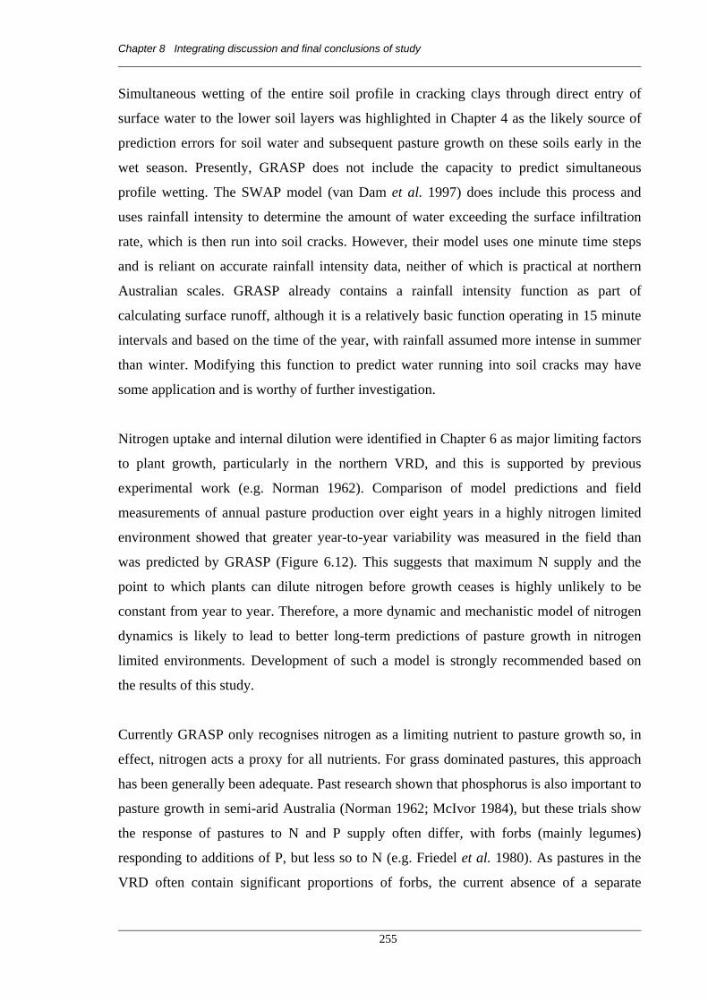
Chapter 8 Integrating discussion and final conclusions of study
255
Simultaneous wetting of the entire soil profile in cracking clays through direct entry of
surface water to the lower soil layers was highlighted in Chapter 4 as the likely source of
prediction errors for soil water and subsequent pasture growth on these soils early in the
wet season. Presently, GRASP does not include the capacity to predict simultaneous
profile wetting. The SWAP model (van Dam et al. 1997) does include this process and
uses rainfall intensity to determine the amount of water exceeding the surface infiltration
rate, which is then run into soil cracks. However, their model uses one minute time steps
and is reliant on accurate rainfall intensity data, neither of which is practical at northern
Australian scales. GRASP already contains a rainfall intensity function as part of
calculating surface runoff, although it is a relatively basic function operating in 15 minute
intervals and based on the time of the year, with rainfall assumed more intense in summer
than winter. Modifying this function to predict water running into soil cracks may have
some application and is worthy of further investigation.
Nitrogen uptake and internal dilution were identified in Chapter 6 as major limiting factors
to plant growth, particularly in the northern VRD, and this is supported by previous
experimental work (e.g. Norman 1962). Comparison of model predictions and field
measurements of annual pasture production over eight years in a highly nitrogen limited
environment showed that greater year-to-year variability was measured in the field than
was predicted by GRASP (Figure 6.12). This suggests that maximum N supply and the
point to which plants can dilute nitrogen before growth ceases is highly unlikely to be
constant from year to year. Therefore, a more dynamic and mechanistic model of nitrogen
dynamics is likely to lead to better long-term predictions of pasture growth in nitrogen
limited environments. Development of such a model is strongly recommended based on
the results of this study.
Currently GRASP only recognises nitrogen as a limiting nutrient to pasture growth so, in
effect, nitrogen acts a proxy for all nutrients. For grass dominated pastures, this approach
has been generally been adequate. Past research shown that phosphorus is also important to
pasture growth in semi-arid Australia (Norman 1962; McIvor 1984), but these trials show
the response of pastures to N and P supply often differ, with forbs (mainly legumes)
responding to additions of P, but less so to N (e.g. Friedel et al. 1980). As pastures in the
VRD often contain significant proportions of forbs, the current absence of a separate

Chapter 8 Integrating discussion and final conclusions of study
256
phosphorus supply index when calculating pasture growth is another factor likely to lead to
prediction errors.
8.4 Recommendations for future work
The previous section discussed the limitations of the field data available for accurate
calibration of GRASP in the VRD, and limitations of the model structure itself. During this
discussion, a number of recommendations for improving the structure of the model were
made to address these limitations. Recommendations fall into two categories: field studies
to improve calibration of the current model; and improvements to model structure. These
are summarised here.
Field studies to improve model calibration
• Testing model performance with field data collected during low rainfall years;
• expanding the number of land systems for which calibration data is available;
• defining the water holding capacity of cracking clay soils more precisely; and
• increasing the spatial intensity of data collection on nitrogen supply and internal plant
dilution.
Improvements to model structure
• Simulating separate biomass pools for perennial grasses and ephemeral species;
• developing a dynamic model for year-to-year variation in nitrogen supply and dilution;
• modifying the rainfall intensity and runoff components to simulate simultaneous
wetting of the whole soil profile in cracking clays; and
• incorporating a phosphorus index to better describe the effect of nutrient supply on
pasture growth.
These lists are not exhaustive and other less critical suggestions for future work are made
throughout the thesis.
This section has recommended a series of future research projects aimed at improving the
capability of GRASP when predicting pasture growth in the VRD, and some of these
recommendations include modifications to the model structure. One consequence of
increasing the complexity of the model by including these recommended changes is the

Chapter 8 Integrating discussion and final conclusions of study
257
effect on its calibration. A more complex model requires a larger number of parameters to
be calibrated, and therefore more field data to derive values for these parameters. Thus,
increasing the complexity of GRASP must be balanced against the additional effort
required to calibrate it so that the model become more useful, rather than more accurate but
less able to be calibrated and applied.
8.5 Final conclusion
The capacity to predict pasture growth in the VRD has now been developed and tested,
overcoming the lack of measured pasture production data available for the VRD.
Predictions can now account for variability in pasture growth due to:
• soil type;
• pasture species composition;
• climate regime; and
• time.
Limitations in the ability to predict pasture growth have been identified, based primarily on
accounting for the spatial and temporal variation in nitrogen supply and dilution by
pastures. As much of the VRD experiences a nitrogen-induced constraint to pasture
growth, model performance will always be determined by the adequacy of the field data
used to initially describe nitrogen supply, and the ability of the model to predict the
dynamics of this supply over time.
Despite this limitation, the outcome of this study represents an important advance in the
provision of pasture production data for use in the development and analysis of grazing
practices in the Victoria River District.

Appendices
Appendices
Appendix 1 Photographs of study sites and specific events
Plate 1 Nalluvial fl
Plate 2 Cspp. pastu
258
orthern Victoria River District landscape showing escarpment country, woodland plains and
ats.
entral Victoria River District landscape showing cattle grazing Chrysopogon fallax and Iseilema
re on cracking clay soil.

Appendices
259
Plate 3 Southern Victoria River District landscape showing open grassy plains with scattered trees and
occasional rocky basalt outcrops.
Plate 4 Land showing evidence of past heavy grazing: bare and scalded ground, dead trees, and annual
pasture species.

Appendices
260
Plate 5 Fencing a study site to exclude cattle from grazing.
Plate 6 Burning to remove carryover material at commencement of the study period (Site 16).
Plate 7 Marking out sampling cells at site establishment (Site 2).

Appendices
261
Plate 8 a) Bulk density sampling in soil profile pit; and b) hand-augering soil moisture cores during field
measurements.
Plate 9 a) Measuring perennial grass basal area using a 5-point frame; and b) pasture sampling during field
measurements.
a. b.
a. b.

Appendices
262
Plate 10 Red earth overlying basalt (Site 19).
Plate 11 Red earth overlying limestone (Site 11).

Appendices
263
Plate 12 Cracking clay overlying basalt (Site 4).
Plate 13 Alluvial cracking clay (Site 7).

Appendices
264
Plate 14 Barley Mitchell grass pasture (Site 18).
Plate 15 Overhead view of 1m2 quadrat in a) barley Mitchell grass pasture (Site 18); and b) ribbon grass
pasture (Site 8).
Plate 16 Ribbon grass pasture (Site 8).
a. b.

Appendices
265
Plate 17 White grass pasture (Site 14).
Plate 18 Overhead view of 1m2 quadrat in a) white grass pasture (Site 14); and b) annual short grass pasture
(Site 1).
Plate 19 Annual short grass pasture (Site 1).
a. b.

Appendices
266
Plate 20 Forb pasture (Site 4).
Plate 21 a) Overhead view of 1m2 quadrat in a forb pasture (Site 4); and b) an example of the abundant,
diverse forbs present at Site 15 on 2 May 1995.
Plate 22 Inundated conditions at Site 15 on 9 March 1995.
a. b.

Appendices
267
Plate 23 Annual short grass pasture early in the wet season with no burning at site establishment (Site 13, 12
Jan 1995).
Plate 24 Overhead view of 1m2 quadrats in an annual short grass pasture (Site 13) during early wet season a)
with no burning at site establishment; and b) after burning to remove carryover material.
Plate 25 Annual short grass pasture early in the wet season after site burnt to remove carryover material (Site
13, 9 Jan 1996). Fire most likely destroyed much of the seed bank, resulting in poor germination.
a. b.

Appendices
268
Appendix 2 Study sites classified according to previous resource
inventories of the VRD
A number of systems exist for classification of land in the VRD using soil, vegetation and
topography. These have been described in Section 2.1 and 2.3.3 of Chapter 2. Each site in
this study has been classified using these systems so results can be easily compared with
future work (Table 9.1 to Table 9.4).
Table 9.1 Study sites classified using: 1 Perry (1970); 2 Stewart et al. (1970); and 3 DIPE (unpublished).
Site Code Pasture Land 1 Land System 2 Land Unit 3 Geology 3
1 An Hilly Country with Useful Lowlands Antrim G6a Basalt
2 An Hilly Country with Useful Lowlands Antrim G6a Basalt
3 Wv Mitchell and Other Grass Plains Wave Hill G6a Basalt
4 Wv Mitchell and Other Grass Plains Wave Hill G6a Basalt
5 Wv Mitchell and Other Grass Plains Wave Hill G6a Basalt
6 Wv Mitchell and Other Grass Plains Wave Hill G6a Basalt
7 A Mitchell and Other Grass Plains Argyle L7l Alluvium
8 A Mitchell and Other Grass Plains Argyle L7l Alluvium
9 A Mitchell and Other Grass Plains Argyle L7l Alluvium
10 A Mitchell and Other Grass Plains Argyle L7l Alluvium
11 Hu Hilly Country with Useful Lowlands Humbert G6d2 Limestone
12 D Tippera Tall Grass Plains Dinnabung G6d2 Limestone
13 Hu Hilly Country with Useful Lowlands Humbert G5d Limestone
14 D Tippera Tall Grass Plains Dinnabung G5d Limestone
15 Iv Blue Grass Plains Ivanhoe L7l Alluvium
16 Iv Blue Grass Plains Ivanhoe L7l Alluvium
17 Wv Mitchell and Other Grass Plains Wave Hill G6a Basalt
18 Wv Mitchell and Other Grass Plains Wave Hill L6a3 Basalt
19 An Hilly Country with Useful Lowlands Antrim G5a9 Basalt
20 Iv Blue Grass Plains Ivanhoe L7l* Alluvium
21 Iv Blue Grass Plains Ivanhoe L7l* Alluvium

Appendices
269
Table 9.2 Study sites classified according to: 1 Northcote (1979); 2 Northcote et al. (1975); 3 Stace et al.
(1968); 4 Isbell (1996); 5 McDonald et al. (1990).
Site No.
Factual Key 1
Soil Texture 1
A Description of Aust. Soils 2
Handbook of Aust. Soils 3
Classification 4 Landform 5
1 Gn 3.12 Gradational Red Smooth-ped Earths Euchrozems Dermosols Hills
2 Gn 3.12 Gradational Red Smooth-ped Earths Euchrozems Dermosols Hills
3 Ug 5.37 Uniform Red Self-mulching
Cracking Clays
Red clays Vertosols Plains
4 Ug 5.37 Uniform Red Self-mulching
Cracking Clays
Red clays Vertosols Plains
5 Ug 5.32 Uniform Brown Self-mulching
Cracking Clays
Brown clays Vertosols Plains
6 Ug 5.37 Uniform Red Self-mulching
Cracking Clays
Red clays Vertosols Plains
7 Ug 5.24 Uniform Grey Self-mulching
Cracking Clays
Grey clays Vertosols Plains
8 Ug 5.24 Uniform Grey Self-mulching
Cracking Clays
Grey clays Vertosols Plains
9 Ug 5.24 Uniform Grey Self-mulching
Cracking Clays
Grey clays Vertosols Plains
10 Ug 5.24 Uniform Grey Self-mulching
Cracking Clays
Grey clays Vertosols Plains
11 Gc 1.22 Gradational Calcareous earths Solonized brown
soils
Calcarosols Plains
12 Gn 3.12 Gradational Red Smooth-ped Earths Euchrozems Dermosols Plains
13 Gn 3.12 Gradational Red Smooth-ped Earths Euchrozems Dermosols Rises
14 Gn 2.13 Gradational Red Massive Earths Calcareous red
earths
Kandosols Rises
15 Ug 5.38 Uniform Red Self-mulching
Cracking Clays
Red clays Vertosols Plains
16 Ug 5.24 Uniform Grey Self-mulching
Cracking Clays
Grey clays Vertosols Plains
17 Ug 5.32 Uniform Brown Self-mulching
Cracking Clays
Brown clays Vertosols Plains
18 Ug 5.37 Uniform Red Self-mulching
Cracking Clays
Red clays Vertosols Plains
19 Gn 3.12 Gradational Red Smooth-ped Earths Euchrozems Dermosols Hills
20 Ug 5.24 Uniform Grey Self-mulching
Cracking Clays
Grey clays Vertosols Plains
21 Ug 5.24 Uniform Grey Self-mulching
Cracking Clays
Grey clays Vertosols Plains

Appendices ------------------------------------------------------------------------------------------------------------------------------------------ Table 9.3 Study sites classified according to Wilson et al. (1990).
____
NOTE: This table is included on page 270 in the print copy of the thesisheld in the University of Adelaide Library.
_________________________________________________________________ 270

Appendices ------------------------------------------------------------------------------------------------------------------------------------------ Table 9.4 Study sites classified according to Tothill and Gillies (1992).
____
NOTE: This table is included on page 271 in the print copy of the thesisheld in the University of Adelaide Library.
_________________________________________________________________ 271

Appendices
272
Appendix 3 Results of soil chemistry analysis
Soil chemical properties were measured for the 0-10cm and 10-20cm soil layers (Section 3.3.5) and full results are presented here. Summary
values appear in the main body of the thesis.
Table 9.5 Laboratory analysis results of soil samples from sites located on red earths overlying basalt.
Site Depth pH1 EC2 Cl3 C Sand4 F Sand5 Silt6 Clay7 Ca8 Mg9 Na10 K11 ECEC12 OC13 NO3-N14 P15 SO4-S16 N(t)17 P(t)18 K(t)19 S(t)20 Cu21 Zn22 Mn23
1 0-10cm 7.5 0.05 1.0 17 44 10 31 10.0 19.0 0.07 1.30 30 0.73 2.0 6.0 3.0 0.05 0.022 2.280 0.014 2.40 0.89 32.0
10-20cm 7.7 0.04 1.0 15 39 13 35 12.0 21.0 0.13 0.52 34 0.64 1.0 2.0 6.0 0.03 0.016 2.050 0.014 2.20 2.20 23.0
2 0-10cm 7.8 0.02 1.0 23 45 8 26 11.0 16.0 0.10 0.74 28 0.51 1.0 6.0 2.0 0.04 0.025 2.100 0.013 2.00 0.44 24.0
10-20cm 7.5 0.03 1.0 14 40 12 35 13.0 19.0 0.15 0.58 33 0.53 1.0 4.0 4.0 0.03 0.022 2.000 0.016 5.00 18.00 5.1
19 0-10cm 7.3 0.06 1.0 14 47 14 27 13.0 14.0 0.07 0.76 28 0.67 1.0 13.0 11.0 0.03 0.031 1.690 0.019 2.00 3.90 81.0
10-20cm 7.2 0.08 1.0 13 37 12 41 15.0 17.0 0.13 0.49 33 0.69 1.0 6.0 15.0 0.04 0.021 1.380 0.020 2.70 3.10 83.0
Units of measurement in Table 9.5 to Table 9.8 1 pH - soil pH 9 Mg - magnesium (mequiv/100g) 17 N(t) - total nitrogen (%) 2 EC - electrical conductivity (dS m–1) 10 Na - sodium (mequiv/100g) 18 P(t) - total phosphorus (%) 3 Cl - soluble chloride (mg kg–1) 11 K - potassium (mequiv/100g) 19 K(t) - total potassium (%) 4 C Sand - coarse sand fraction (%) 12 ECEC - effective cation exchange capacity (mequiv/100g, Ca + Mg + Na + K) 5 F Sand - fine sand fraction (%) 13 OC - organic carbon (%) 20 S(t) - total sulphur (%) 6 Silt - silt fraction (%) 14 NO3-N - nitrate-nitrogen (mg kg–1) 21 Cu - copper (mg kg–1) 7 Clay - clay fraction (%) 15 P - phosphorus, bicarbonate extractable (Colwell) (mg kg–1) 22 Zn - zinc (mg kg–1) 8 Ca - calcium (mequiv/100g) 16 SO4-S – sulphate-sulphur, extractable (mg kg–1) 23 Mn - Manganese (mg kg–1)
Standard analysis methods of Rayment and Higginson (1982).

Appendices
273
Table 9.6 Laboratory analysis results of soil samples from sites located on red earths overlying limestone.
Site Depth pH1 EC2 Cl3 C Sand4 F Sand5 Silt6 Clay7 Ca8 Mg9 Na10 K11 ECEC12 OC13 NO3-N14 P15 SO4-S16 N(t)17 P(t)18 K(t)19 S(t)20 Cu21 Zn22 Mn23
11 0-10cm 8.3 0.09 1.0 2 55 12 33 16.0 5.1 0.03 0.79 22 0.97 1.0 11.0 2.0 0.06 0.020 2.660 0.019 0.47 0.64 15.0
10-20cm 8.4 0.12 1.0 3 51 10 38 28.0 5.0 0.05 0.64 34 0.81 1.0 8.0 2.0 0.02 0.022 2.730 0.016 0.91 0.80 13.0
12 0-10cm 7.6 0.03 1.0 3 33 15 50 9.5 4.9 0.04 1.00 15 1.10 1.0 13.0 4.0 0.05 0.021 3.060 0.015 1.50 0.50 35.0
10-20cm 7.6 0.03 1.0 2 27 13 60 11.0 4.8 0.02 0.92 17 0.89 1.0 8.0 6.0 0.04 0.020 3.100 0.014 1.50 0.31 31.0
13 0-10cm 7.3 0.04 1.0 3 53 14 31 8.9 3.6 0.03 0.76 13 0.73 1.0 13.0 5.0 0.04 0.018 1.916 0.014 0.51 5.48 18.0
10-20cm 7.9 0.03 3.0 2 44 9 43 14.0 4.4 0.04 0.66 19 0.70 1.0 12.0 5.0 0.03 0.017 2.300 0.014 0.45 3.50 5.8
14 0-10cm 7.3 0.03 3.0 5 57 17 26 5.2 3.3 0.03 0.44 9 0.87 1.0 11.0 4.0 0.03 0.018 1.860 0.013 0.48 3.70 13.0
10-20cm 7.5 0.03 3.0 2 44 10 46 7.2 4.1 0.03 0.66 12 0.76 4.0 5.0 3.0 0.04 0.018 2.390 0.014 0.77 1.20 6.5
Units of measurement are shown in the footnote of Table 9.5.
Table 9.7 Laboratory analysis results of soil samples from sites located on cracking clays overlying basalt.
Site Depth pH1 EC2 Cl3 C Sand4 F Sand5 Silt6 Clay7 Ca8 Mg9 Na10 K11 ECEC12 OC13 NO3-N14 P15 SO4-S16 N(t)17 P(t)18 K(t)19 S(t)20 Cu21 Zn22 Mn23
3 0-10cm 8.3 0.10 1.0 4 29 13 52 23.0 20.0 0.68 1.10 45 0.53 1.0 8.0 2.0 0.03 0.013 1.210 0.013 1.50 0.83 14.0
10-20cm 8.7 0.12 1.0 6 26 12 56 25.0 21.0 1.30 0.90 48 0.59 2.0 6.0 3.0 0.02 0.010 1.150 0.011 1.90 0.85 8.8
4 0-10cm 8.5 0.07 1.0 6 34 10 52 35.0 16.0 0.13 1.00 52 0.45 1.0 7.0 2.0 0.03 0.013 1.040 0.011 0.89 0.49 9.2
10-20cm 8.4 0.08 2.0 6 31 10 52 36.0 16.0 0.18 0.93 53 0.36 1.0 7.0 2.0 0.02 0.011 1.000 0.011 1.40 0.89 9.0
5 0-10cm 8.3 0.07 1.0 4 30 12 53 31.0 17.0 0.22 0.97 49 0.37 1.0 7.0 3.0 0.02 0.012 0.661 0.013 1.20 0.64 12.0
10-20cm 8.5 0.08 1.0 3 30 12 55 31.0 18.0 0.33 0.77 50 0.41 1.0 7.0 4.0 0.02 0.009 0.627 0.012 1.20 0.58 9.5
6 0-10cm 8.0 0.04 1.0 4 35 13 50 24.0 16.0 0.06 1.30 41 0.48 1.0 8.0 2.0 0.02 0.012 1.020 0.013 5.20 19.00 13.0
10-20cm 7.9 0.03 1.0 4 34 11 52 28.0 18.0 0.13 1.10 47 0.41 1.0 6.0 2.0 0.03 0.009 1.030 0.010 1.40 0.86 19.0
17 0-10cm 7.3 0.07 1.0 10 29 15 48 23.0 16.0 0.22 0.81 40 0.64 1.0 13.0 11.0 0.03 0.014 0.868 0.015 5.20 15.00 131.0
10-20cm 7.2 0.09 1.0 9 27 17 50 25.0 17.0 0.30 0.56 43 0.50 1.0 8.0 15.0 0.02 0.011 0.839 0.020 4.10 21.00 77.0
18 0-10cm 7.8 0.09 1.0 6 26 13 57 34.0 19.0 0.19 1.30 54 0.55 2.0 13.0 18.0 0.03 0.012 0.905 0.013 1.00 5.00 43.0
10-20cm 7.7 0.08 1.0 6 25 13 56 34.0 19.0 0.23 1.10 54 0.42 1.0 8.0 14.0 0.02 0.010 0.875 0.012 0.87 5.90 36.0
Units of measurement are shown in the footnote of Table 9.5.

Appendices
274
Table 9.8 Laboratory analysis results of soil samples from sites located on cracking clays of alluvial origin.
Site Depth pH1 EC2 Cl3 C Sand4 F Sand5 Silt6 Clay7 Ca8 Mg9 Na10 K11 ECEC12 OC13 NO3-N14 P15 SO4-S16 N(t)17 P(t)18 K(t)19 S(t)20 Cu21 Zn22 Mn23
7 0-10cm 8.3 0.06 1.0 1 35 13 51 28.0 12.0 0.38 0.86 41 0.55 1.0 8.0 3.0 0.02 0.010 1.320 0.011 1.00 1.80 14.0
10-20cm 8.4 0.06 1.0 1 33 13 53 29.0 12.0 0.59 0.75 42 0.47 1.0 8.0 3.0 0.02 0.008 1.310 0.010 1.10 1.10 11.0
8 0-10cm 8.3 0.10 1.0 3 36 14 50 28.0 9.7 0.19 0.96 39 0.59 2.0 8.0 4.0 0.04 0.014 1.620 0.013 1.40 0.88 12.0
10-20cm 8.5 0.09 1.0 2 33 12 52 30.0 11.0 0.23 0.83 42 0.47 1.0 7.0 5.0 0.02 0.013 1.630 0.010 1.20 0.58 9.0
9 0-10cm 8.1 0.05 1.0 2 40 3 57 23.0 8.9 0.17 0.45 33 0.45 1.0 4.0 31.0 0.02 0.007 0.360 0.010 1.00 1.10 30.0
10-20cm 8.2 0.04 1.0 2 39 13 48 25.0 9.2 0.27 0.33 35 0.33 1.0 4.0 4.0 0.01 0.006 0.324 0.009 1.00 0.87 16.0
10 0-10cm 8.2 0.04 1.0 2 42 13 44 22.0 9.1 0.22 0.41 32 0.45 1.0 4.0 4.0 0.02 0.005 0.334 0.009 1.00 0.96 26.0
10-20cm 8.1 0.04 1.0 2 40 13 46 23.0 9.0 0.26 0.35 33 0.33 1.0 3.0 5.0 0.01 0.006 0.317 0.008 0.93 0.70 18.0
15 0-10cm 8.7 0.06 1.0 3 20 16 61 28.0 14.0 0.50 0.62 43 0.67 1.0 7.0 6.0 0.04 0.017 1.790 0.011 0.62 5.20 3.6
10-20cm 8.9 0.07 1.0 3 20 14 63 27.0 14.0 0.94 0.50 42 0.66 5.0 7.0 2.0 0.03 0.016 1.740 0.011 0.54 2.60 2.5
16 0-10cm 7.9 0.03 1.0 6 40 11 46 20.0 16.0 0.08 0.63 37 0.70 1.0 6.0 1.0 0.04 0.008 0.989 0.011 0.53 5.80 4.8
10-20cm 8.1 0.03 1.0 6 39 11 46 20.0 16.0 0.08 0.65 37 0.45 1.0 4.0 1.0 0.03 0.008 1.020 0.011 0.53 7.80 5.0
20 0-10cm 8.0 0.07 1.0 3 44 18 39 20.0 7.5 0.08 0.49 28 0.58 2.0 10.0 7.0 0.03 0.011 0.519 0.012 0.59 7.20 20.0
10-20cm 8.4 0.07 1.0 3 41 15 42 21.0 8.6 0.13 0.34 30 0.51 1.0 8.0 4.0 0.03 0.009 0.524 0.011 0.47 5.10 10.0
21 0-10cm 6.9 0.07 6.0 4 48 12 36 10.0 7.3 0.10 0.62 18 0.48 1.0 6.0 9.0 0.02 0.010 0.507 0.011 0.89 5.70 119.0
10-20cm 7.1 0.04 1.0 4 46 13 39 11.0 7.2 0.11 0.48 19 0.37 1.0 4.0 4.0 0.01 0.007 0.491 0.009 0.65 4.60 47.0
Units of measurement are shown in the footnote of Table 9.5.

Appendices
275
Many of the soil nutrient analysis results in Table 9.5 to Table 9.8 are reported as weight of
nutrient per unit weight of soil (i.e. mg/kg, equivalent to ‘parts per million’). Converting
these values to weight of nutrient per unit area (i.e. kg/ha) provides quantitative values for
the amount of nutrients present in the landscape. The major nutrients of carbon, nitrogen
and phosphorus have been converted in this way and are presented in Table 9.9. The
conversion procedure is detailed in Dalgliesh and Foale (1998).
Table 9.9 Amount of soil nutrients present in surface layers of study sites. (Table continued overleaf)
Site Depth OC 1 NO3-N 2 N(t) 3 P(t) 4 C:N ratio 5
Red earths overlying basalt
1 0-10cm 10512 2.88 720 317 14.6
10-20cm 9664 1.51 453 242 21.3
20-30cm 10560 1.65 495 264 21.3
2 0-10cm 7548 1.48 592 370 12.8
10-20cm 7632 1.44 432 317 17.7
20-30cm 8003 1.51 453 332 17.7
19 0-10cm 10586 1.58 474 490 22.3
10-20cm 9867 1.43 572 300 17.3
20-30cm 10419 1.51 604 317 17.3
Red earths overlying limestone
11 0-10cm 15423 1.59 954 318 16.2
10-20cm 11988 1.48 296 326 40.5
20-30cm 11988 1.48 296 326 40.5
12 0-10cm 16060 1.46 730 307 22.0
10-20cm 14062 1.58 632 316 22.3
20-30cm 13083 1.47 588 294 22.3
13 0-10cm 12410 1.70 680 306 18.3
10-20cm 11550 1.65 495 280 23.3
20-30cm 11830 1.69 507 287 23.3
14 0-10cm 13659 1.57 471 283 29.0
10-20cm 11932 6.28 628 283 19.0
20-30cm 12768 6.72 672 302 19.0
Units of measurement: 1 OC - organic carbon (kg/ha) 2 NO3-N - nitrate-nitrogen (kg/ha) 3 N(t) - total nitrogen (kg/ha) 4 P(t) - total phosphorus (kg/ha) 5 C:N ratio – carbon to nitrogen ratio

Appendices
276
Table 9.9 (cont.) (Table continued overleaf)
Site Depth OC 1 NO3-N 2 N(t) 3 P(t) 4 C:N ratio 5
Cracking clays overlying basalt
3 0-10cm 6254 1.18 354 153 17.7
10-20cm 7198 2.44 244 122 29.5
20-30cm 8909 3.02 302 151 29.5
4 0-10cm 6075 1.35 405 176 15.0
10-20cm 5148 1.43 286 157 18.0
20-30cm 5472 1.52 304 167 18.0
5 0-10cm 5143 1.39 278 167 18.5
10-20cm 6109 1.49 298 134 20.5
20-30cm 6232 1.52 304 137 20.5
6 0-10cm 6048 1.26 252 151 24.0
10-20cm 5822 1.42 426 128 13.7
20-30cm 6355 1.55 465 139 13.7
17 0-10cm 8640 1.35 405 189 21.3
10-20cm 7350 1.47 294 162 25.0
20-30cm 7850 1.57 314 173 25.0
18 0-10cm 7095 2.58 387 155 18.3
10-20cm 5628 1.34 268 134 21.0
20-30cm 5838 1.39 278 139 21.0

Appendices
277
Table 9.9 (cont.)
Site Depth OC 1 NO3-N 2 N(t) 3 P(t) 4 C:N ratio 5
Cracking clays of alluvial origin
7 0-10cm 8250 1.50 300 150 27.5
10-20cm 6580 1.40 280 112 23.5
20-30cm 6674 1.42 284 114 23.5
8 0-10cm 9086 3.08 616 216 14.8
10-20cm 7896 1.68 336 218 23.5
20-30cm 7896 1.68 336 218 23.5
9 0-10cm 6840 1.52 304 106 22.5
10-20cm 5907 1.79 179 107 33.0
20-30cm 5775 1.75 175 105 33.0
10 0-10cm 7110 1.58 316 79 22.5
10-20cm 5049 1.53 153 92 33.0
20-30cm 5709 1.73 173 104 33.0
15 0-10cm 10050 1.50 600 255 16.7
10-20cm 10362 7.85 471 251 22.0
20-30cm 9702 7.35 441 235 22.0
16 0-10cm 9240 1.32 528 106 17.5
10-20cm 6930 1.54 462 123 15.0
20-30cm 6930 1.54 462 123 15.0
20 0-10cm 9744 3.36 504 185 19.3
10-20cm 9180 1.80 540 162 17.0
20-30cm 9180 1.80 540 162 17.0
21 0-10cm 7296 1.52 304 152 24.0
10-20cm 5624 1.52 152 106 37.0
20-30cm 5624 1.52 152 106 37.0

Appendices
278
Appendix 4 Plant species nomenclature
Species identification nomenclature used in this study is taken from Dunlop (1990) and
Barritt (1996).
Table 9.10 Plant species nomenclature for all individual species presented in this study.
Abelmoschus ficulneus (L.) Wight & Arn. ex Wight
Abutilon andrewsianum W. Fitzg.
Abutilon otocarpum F. Muell.
Aristida holathera Domin
Aristida inaequiglumis Domin
Aristida latifolia Domin
Astrebla elymoides F. Muell.
Astrebla pectinata (Lindley) F. Muell. ex Benth.
Astrebla squarrosa C. Hubb.
Atalaya hemiglauca (F. Muell.) F. Muell. ex Benth.
Basilicum polystachyon (L.) Moench
Boerhavia dominii Meikle & Hewson
Bonamia pannosa (R. Br.) Hallier f.
Brachyachne convergens (F. Muell.) Stapf
Carissa lanceolata R. Br.
Chionachne hubbardiana Henrard
Chrysogonum trichodesmoides (F. Muell.) F. Muell.
Chrysopogon fallax S.T. Blake
* Citrullus colocynthis (L.) Schrader
Corymbia terminalis (F. Muell.) K.D. Hill & L.A.S. Johnson
Crotalaria medicaginea Lam.
Dactyloctenium radulans (R. Br.) Beauv.
Dichanthium fecundum S.T. Blake
Dichanthium sericeum (R. Br.) A. Camus
Echinochloa elliptica Michael & Vickery
Enneapogon polyphyllus (Domin) N. Burb.
Eriachne aristidae F. Muell.
Eucalyptus brevifolia F. Muell.
Eucalyptus pruinosa Schauer
Eulalia aurea (Bory) Kunth
Euphorbia schultzii Benth.
Euphorbia vachellii Hook. & Arn.
Evolvulus alsinoides L.
Flemingia pauciflora Benth.
Gomphrena canescens R. Br.
Gossypium australe F. Muell.
Grevillea striata R. Br.
Hakea arborescens R. Br.
Heliotropium tenuifolium R. Br.
Heteropogon contortus (L.) Beauv. ex Roemer & Schultes
Indigofera colutea (Burman f.) Merrill
Indigofera hirsuta L.
Indigofera trita L. f.
Ipomoea polymorpha Roemer & Schultes
Iseilema fragile S.T. Blake
Iseilema vaginiflorum Domin
Jacquemontia browniana Ooststr.
Lysiphyllum cunninghamii (Benth.) De Wit
Neptunia monosperma F. Muell.
Panicum decompositum R. Br.
Phyllanthus urinaria L.
Polymeria ambigua R. Br.
Psoralea pustulata F. Muell.
Ptilotus exaltatus Nees
Rhyncosia australis Benth.
Rhyncosia minima (L.) DC.
Salsola kali L.
Sehima nervosum (Rottler.) Stapf
Sesbania cannabina (Retz.) Poiret
Sida cleistocalyx F. Muell.
Sorghum stipoideum (Ewart & J.W. White) C. Gardner &
C. Hubb
Sporobolus australasicus Domin
* Stylosanthes humilis Kunth
Tephrosia macrocarpa Benth.
Terminalia arostrata Ewart & O. Davies
Terminalia canescens (DC.) Radlk.
Terminalia volucris R. Br. ex Benth.
Trichodesma zeylanicum (Burman f.) R. Br.
(* denotes introduced species)

Appendices
279
Appendix 5 Description of complete species composition at the study sites
The entire floristic composition of each site was described once (July 1995). A botanist
(Jack Cusack, CSIRO Division of Wildlife and Ecology) identified all tree, shrub, and
pasture species present in the immediate area, and provided an indication of their
abundance. Table 9.11 shows an example of the floristic description for a site (Site 1).
Table 9.11 Complete list of plant species present at Site 1, July 1995.
Abundance Scientific Name Common Name Common Patchy Sparse
Brachyachne convergens Native couch X
Aristida latifolia Feathertop wiregrass X
Enneapogon polyphyllus Limestone grass X
Indigofera trita X
Salsola kali Roly poly X
Sida cleistocalyx X
Abutilon otocarpum Desert lantern X
Abutilon andrewsianum X
Astrebla elymoides Weeping Mitchell grass X
Atalaya hemiglauca Whitewood X
Boerhavia dominii Boerhavia X
Carissa lanceolata Conkerberry X
Chrysopogon fallax Golden beard grass X
Citrullus colocynthis Bush cucumber X
Corymbia terminalis Northern bloodwood X
Crotalaria medicaginea Rattlepod X
Dichanthium sericeum Queensland bluegrass X
Echinochloa elliptica Nasty grass X
Euphorbia vachellii X
Evolvulus alsinoides X
Grevillea striata X
Heliotropium tenuifolium Heliotrope X
Indigofera colutea X
Iseilema fragile Flinders grass X
Iseilema vaginiflorum Red flinders grass X
Jacquemontia browniana Snake stem X
Panicum decompositum Native millet X
Phyllanthus urinaria Phyllanthus X
Psoralea pustulata X
Rhyncosia minima Native rhyncosia X
Sporobolus australasicus Fairy grass X
Tephrosia macrocarpa X
Terminalia arostrata Nutwood X

Appendices
280
Appendix 6 Pasture field data in addition to that presented in Chapter 3
Most pasture data from the study sites are presented in Section 3.4.3. Results of species
composition and nitrogen dynamics from three sites representative of each group appear in
the relevant sections (Section 3.4.3.4 to Section 3.4.3.8). Data from sites not included in
those sections are presented here. In addition, data on the flow of dry matter through the
three biomass pools (green material, dead material and detached litter) are also presented.
Figure 9.1 Pasture composition results not presented in Chapter 3. Error bars indicate the standard error of
the site mean for total standing dry matter at each sampling time (harvest). (Figure continued overleaf)
Site 3
0
1000
2000
3000
4000
Jul-93 Oct-93 Jan-94 Apr-94 Jul-94 Oct-94 Jan-95 Apr-95 Jul-95 Oct-95
TSD
M (k
g/ha
)
ForbsAnnual GrassPerennial Grass
Site 7
0
1000
2000
3000
4000
Jul-93 Oct-93 Jan-94 Apr-94 Jul-94 Oct-94 Jan-95 Apr-95 Jul-95 Oct-95
TSD
M (k
g/ha
)
ForbsAnnual GrassPerennial Grass
Site 16
0
1000
2000
3000
4000
Jul-94 Oct-94 Jan-95 Apr-95 Jul-95 Oct-95 Jan-96 Apr-96 Jul-96 Oct-96
TSD
M (k
g/ha
)
ForbsAnnual GrassPerennial Grass

Appendices
281
Figure 9.1 (cont.)
Site 11
0
1000
2000
3000
4000
Jul-93 Oct-93 Jan-94 Apr-94 Jul-94 Oct-94 Jan-95 Apr-95 Jul-95 Oct-95
TSD
M (k
g/ha
)
ForbsAnnual GrassPerennial Grass
Site 12
0
1000
2000
3000
4000
Jul-93 Oct-93 Jan-94 Apr-94 Jul-94 Oct-94 Jan-95 Apr-95 Jul-95 Oct-95
TSD
M (k
g/ha
)
ForbsAnnual GrassPerennial Grass
Site 19
0
1000
2000
3000
4000
Jul-94 Oct-94 Jan-95 Apr-95 Jul-95 Oct-95 Jan-96 Apr-96 Jul-96 Oct-96
TSD
M (k
g/ha
)
ForbsAnnual GrassPerennial Grass

Appendices
282
Figure 9.2 Pasture nitrogen contents (dashed lines) and nitrogen uptake (vertical bars) of sites not presented
in Chapter 3. (Figure continued overleaf)
The dotted lines represent expected nitrogen contents during periods where no data was collected (explained
in the text at end of Section 3.4.3.4).
Site 3
0
10
20
30
40
50
60
Jul-93 Oct-93 Jan-94 Apr-94 Jul-94 Oct-94 Jan-95 Apr-95 Jul-95 Oct-95
N U
ptak
e (k
g/ha
)
-4.0
-3.0
-2.0
-1.0
0.0
1.0
2.0
3.0
4.0
N C
onte
nt (%
)
Site 7
0
10
20
30
40
50
60
Jul-93 Oct-93 Jan-94 Apr-94 Jul-94 Oct-94 Jan-95 Apr-95 Jul-95 Oct-95
N U
ptak
e (k
g/ha
)
-4.0
-3.0
-2.0
-1.0
0.0
1.0
2.0
3.0
4.0
N C
onte
nt (%
)
Site 16
0
10
20
30
40
50
60
Jul-94 Oct-94 Jan-95 Apr-95 Jul-95 Oct-95 Jan-96 Apr-96 Jul-96 Oct-96
N U
ptak
e (k
g/ha
)
-4.0
-3.0
-2.0
-1.0
0.0
1.0
2.0
3.0
4.0N
Con
tent
(%)

Appendices
283
Figure 9.2 (cont.)
Site 11
0
10
20
30
40
50
60
Jul-93 Oct-93 Jan-94 Apr-94 Jul-94 Oct-94 Jan-95 Apr-95 Jul-95 Oct-95
N U
ptak
e (k
g/ha
)
-4.0
-3.0
-2.0
-1.0
0.0
1.0
2.0
3.0
4.0
N C
onte
nt (%
)
Site 12
0
10
20
30
40
50
60
Jul-93 Oct-93 Jan-94 Apr-94 Jul-94 Oct-94 Jan-95 Apr-95 Jul-95 Oct-95
N U
ptak
e (k
g/ha
)
-4.0
-3.0
-2.0
-1.0
0.0
1.0
2.0
3.0
4.0
N C
onte
nt (%
)Site 19
0
10
20
30
40
50
60
Jul-94 Oct-94 Jan-95 Apr-95 Jul-95 Oct-95 Jan-96 Apr-96 Jul-96 Oct-96
N U
ptak
e (k
g/ha
)
-4.0
-3.0
-2.0
-1.0
0.0
1.0
2.0
3.0
4.0N
Con
tent
(%)

Appendices
284
Appendix 7 Descriptive statistics for total standing dry matter
measurements
Table 9.12 Descriptive statistics for total standing dry matter data collected at each harvest for all sites. Eight
1m2 quadrats were cut at each harvest. All units are kg/ha. (Table continued overleaf)
Site Harvest Date Mean quadrat
yield
Minimum quadrat
yield
Maximum quadrat
yield
Standard error of mean
95% confidence limit of mean
1 1 02/02/1994 735 354 1577 ±140.6 ±332.5
2 11/03/1994 1887 1185 3023 ±215.3 ±509.1
3 05/05/1994 1951 1119 2651 ±165.5 ±391.2
4 14/09/1994 2165 1416 2938 ±204.6 ±483.7
5 04/01/1995 294 87 821 ±92.4 ±218.4
6 14/03/1995 2233 453 4098 ±409.8 ±969.0
7 26/04/1995 2952 1955 4797 ±398.9 ±943.4
8 15/11/1995 Not measured
2 1 02/02/1994 533 185 1263 ±127.3 ±301.0
2 11/03/1994 1013 783 1273 ±66.3 ±156.8
3 04/05/1994 1977 1147 3351 ±238.7 ±564.5
4 14/09/1994 1931 892 2648 ±218.0 ±515.5
5 04/01/1995 71 0 270 ±33.3 ±78.8
6 15/03/1995 2022 462 3508 ±339.3 ±802.3
7 27/04/1995 2424 1427 3434 ±262.9 ±621.6
8 29/11/1995 1413 541 2252 ±193.7 ±458.0
3 1 02/02/1994 1091 754 1615 ±115.8 ±273.7
2 12/03/1994 1430 562 2235 ±178.4 ±421.8
3 04/05/1994 1861 1124 2322 ±132.8 ±314.1
4 15/09/1994 2058 1288 3396 ±277.9 ±657.1
5 04/01/1995 76 31 115 ±9.8 ±23.3
6 14/03/1995 1654 1079 2125 ±122.0 ±288.6
7 26/04/1995 2544 1600 3796 ±308.8 ±730.2
8 17/11/1995 1573 1097 2002 ±97.4 ±230.2
4 1 01/02/1994 1121 745 1696 ±101.7 ±240.4
2 12/03/1994 1807 1395 2618 ±146.4 ±346.3
3 04/05/1994 2343 1805 3122 ±160.6 ±379.7
4 13/09/1994 1232 756 1913 ±150.6 ±356.1
5 05/01/1995 78 21 157 ±20.0 ±47.2
6 13/03/1995 2950 2212 4282 ±294.7 ±696.8
7 27/04/1995 2672 2074 4941 ±327.9 ±775.3
8 15/11/1995 1747 986 3565 ±335.4 ±793.0
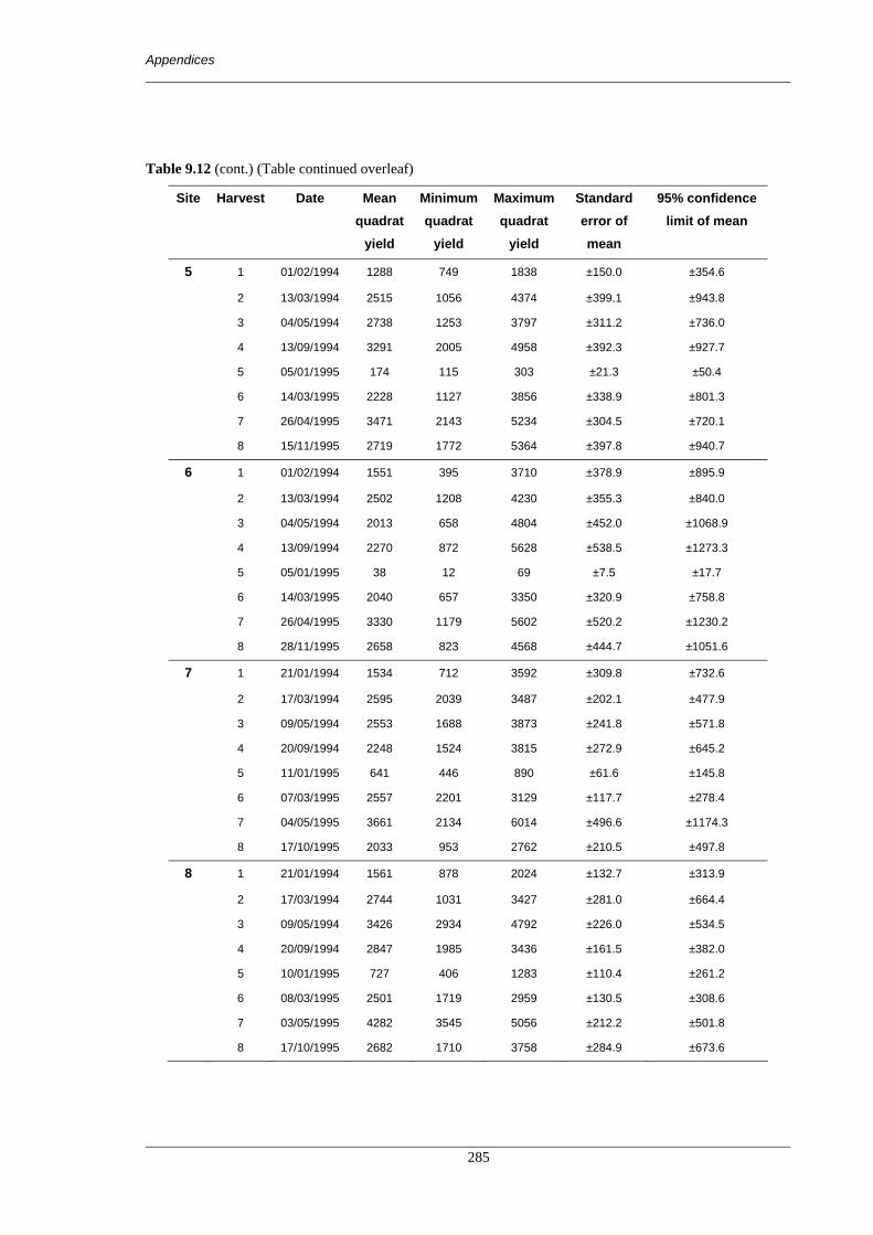
Appendices
285
Table 9.12 (cont.) (Table continued overleaf)
Site Harvest Date Mean quadrat
yield
Minimum quadrat
yield
Maximum quadrat
yield
Standard error of mean
95% confidence limit of mean
5 1 01/02/1994 1288 749 1838 ±150.0 ±354.6
2 13/03/1994 2515 1056 4374 ±399.1 ±943.8
3 04/05/1994 2738 1253 3797 ±311.2 ±736.0
4 13/09/1994 3291 2005 4958 ±392.3 ±927.7
5 05/01/1995 174 115 303 ±21.3 ±50.4
6 14/03/1995 2228 1127 3856 ±338.9 ±801.3
7 26/04/1995 3471 2143 5234 ±304.5 ±720.1
8 15/11/1995 2719 1772 5364 ±397.8 ±940.7
6 1 01/02/1994 1551 395 3710 ±378.9 ±895.9
2 13/03/1994 2502 1208 4230 ±355.3 ±840.0
3 04/05/1994 2013 658 4804 ±452.0 ±1068.9
4 13/09/1994 2270 872 5628 ±538.5 ±1273.3
5 05/01/1995 38 12 69 ±7.5 ±17.7
6 14/03/1995 2040 657 3350 ±320.9 ±758.8
7 26/04/1995 3330 1179 5602 ±520.2 ±1230.2
8 28/11/1995 2658 823 4568 ±444.7 ±1051.6
7 1 21/01/1994 1534 712 3592 ±309.8 ±732.6
2 17/03/1994 2595 2039 3487 ±202.1 ±477.9
3 09/05/1994 2553 1688 3873 ±241.8 ±571.8
4 20/09/1994 2248 1524 3815 ±272.9 ±645.2
5 11/01/1995 641 446 890 ±61.6 ±145.8
6 07/03/1995 2557 2201 3129 ±117.7 ±278.4
7 04/05/1995 3661 2134 6014 ±496.6 ±1174.3
8 17/10/1995 2033 953 2762 ±210.5 ±497.8
8 1 21/01/1994 1561 878 2024 ±132.7 ±313.9
2 17/03/1994 2744 1031 3427 ±281.0 ±664.4
3 09/05/1994 3426 2934 4792 ±226.0 ±534.5
4 20/09/1994 2847 1985 3436 ±161.5 ±382.0
5 10/01/1995 727 406 1283 ±110.4 ±261.2
6 08/03/1995 2501 1719 2959 ±130.5 ±308.6
7 03/05/1995 4282 3545 5056 ±212.2 ±501.8
8 17/10/1995 2682 1710 3758 ±284.9 ±673.6

Appendices
286
Table 9.12 (cont.) (Table continued overleaf)
Site Harvest Date Mean quadrat
yield
Minimum quadrat
yield
Maximum quadrat
yield
Standard error of mean
95% confidence limit of mean
9 1 19/01/1994 826 320 1299 ±112.3 ±265.6
2 18/03/1994 2008 1259 3238 ±213.5 ±504.9
3 10/05/1994 1862 1388 2970 ±171.2 ±404.8
4 21/09/1994 1626 325 3310 ±318.0 ±751.9
5 11/01/1995 546 183 858 ±75.6 ±178.7
6 08/03/1995 2298 1304 4221 ±340.3 ±804.7
7 04/05/1995 2527 1874 3789 ±208.2 ±492.4
8 18/10/1995 1314 651 1568 ±105.0 ±248.4
10 1 18/01/1994 1060 681 1726 ±134.1 ±317.0
2 18/03/1994 2279 1842 3173 ±175.0 ±413.8
3 10/05/1994 2666 963 5343 ±547.2 ±1293.9
4 21/09/1994 1590 1037 2347 ±135.6 ±320.7
5 11/01/1995 476 232 857 ±81.1 ±191.9
6 08/03/1995 2233 1330 3047 ±211.5 ±500.2
7 04/05/1995 2763 1790 4417 ±336.7 ±796.3
8 17/10/1995 1542 1232 2097 ±102.0 ±241.1
11 1 20/01/1994 897 439 1426 ±115.6 ±273.3
2 16/03/1994 2683 1673 3856 ±259.8 ±614.4
3 10/05/1994 2707 1595 5311 ±420.1 ±993.4
4 22/09/1994 2567 1135 4247 ±369.1 ±872.8
5 10/01/1995 700 56 1348 ±145.8 ±344.7
6 06/03/1995 2039 686 3080 ±266.3 ±629.8
7 03/05/1995 2345 1343 3830 ±370.6 ±876.4
8 17/10/1995 2365 786 3060 ±297.2 ±702.8
12 1 20/01/1994 768 66 1621 ±179.2 ±423.7
2 17/03/1994 1923 1162 2563 ±164.8 ±389.6
3 10/05/1994 2418 896 4121 ±365.8 ±865.1
4 22/09/1994 2248 446 4622 ±486.7 ±1150.8
5 12/01/1995 630 133 1647 ±183.7 ±434.4
6 07/03/1995 2003 984 4700 ±413.4 ±977.6
7 03/05/1995 3032 1100 4804 ±477.1 ±1128.1
8 17/10/1995 2537 586 5568 ±717.9 ±1697.5

Appendices
287
Table 9.12 (cont.) (Table continued overleaf)
Site Harvest Date Mean quadrat
yield
Minimum quadrat
yield
Maximum quadrat
yield
Standard error of mean
95% confidence limit of mean
13 1 12/01/1995 518 238 894 ±80.5 ±190.4
2 07/03/1995 2529 1577 3431 ±293.9 ±694.9
3 04/05/1995 2593 1656 3315 ±194.5 ±459.8
4 17/10/1995 2085 1187 4072 ±318.6 ±753.3
5 09/01/1996 132 13 268 ±36.5 ±86.2
6 29/02/1996 530 55 877 ±113.5 ±268.4
7 28/05/1996 854 375 1250 ±100.0 ±236.4
8 26/11/1996 366 116 829 ±80.9 ±191.4
14 1 12/01/1995 316 0 610 ±73.9 ±174.7
2 06/03/1995 1858 1735 1988 ±35.6 ±84.1
3 03/05/1995 2396 187 3503 ±377.9 ±893.7
4 17/10/1995 1627 804 2176 ±181.6 ±429.3
5 10/01/1996 385 181 721 ±72.3 ±171.0
6 29/02/1996 920 151 1509 ±176.7 ±417.7
7 28/05/1996 1531 202 2737 ±310.6 ±734.4
8 26/11/1996 1581 0 2747 ±346.4 ±819.2
15 1 13/01/1995 419 195 655 ±52.3 ±123.6
2 09/03/1995 2758 2025 4118 ±284.1 ±671.9
3 02/05/1995 2696 1339 4985 ±398.0 ±941.2
4 18/10/1995 1965 440 7689 ±851.3 ±2012.9
5 10/01/1996 1071 781 1435 ±75.7 ±179.0
6 28/02/1996 1499 648 2174 ±184.9 ±437.1
7 30/05/1996 2680 1689 4102 ±274.2 ±648.5
8 26/11/1996 1138 0 2402 ±368.8 ±872.2
16 1 13/01/1995 357 129 593 ±57.5 ±135.9
2 09/03/1995 2840 1927 3366 ±160.0 ±378.2
3 02/05/1995 3093 2619 3474 ±91.0 ±215.2
4 18/10/1995 1882 1556 2569 ±112.9 ±266.9
5 10/01/1996 566 370 849 ±68.9 ±162.9
6 28/02/1996 1044 557 1801 ±132.8 ±314.1
7 30/05/1996 2682 1877 4469 ±287.9 ±680.9
8 26/11/1996 Not measured

Appendices
288
Table 9.12 (cont.) (Table continued overleaf)
Site Harvest Date Mean quadrat
yield
Minimum quadrat
yield
Maximum quadrat
yield
Standard error of mean
95% confidence limit of mean
17 1 14/12/1994 160 101 378 ±32.2 ±76.2
2 08/02/1995 1543 1032 2579 ±181.5 ±429.1
3 20/04/1995 2315 877 4645 ±497.4 ±1176.1
4 03/11/1995 1379 573 3183 ±302.6 ±715.6
5 05/01/1996 193 76 311 ±27.6 ±65.3
6 15/02/1996 1053 492 2929 ±276.5 ±653.8
7 06/06/1996 1762 970 3734 ±311.2 ±736.0
8 28/11/1996 1313 794 1976 ±135.4 ±320.2
18 1 15/12/1994 405 115 564 ±46.2 ±109.3
2 08/02/1995 2290 342 3750 ±358.1 ±846.7
3 19/04/1995 3359 2469 5436 ±336.2 ±795.1
4 02/11/1995 2696 1394 3726 ±278.8 ±659.3
5 04/01/1996 360 234 472 ±36.2 ±85.5
6 14/02/1996 1384 940 1848 ±126.0 ±298.0
7 05/06/1996 2254 705 3648 ±432.4 ±1022.5
8 28/11/1996 1521 1044 1981 ±106.5 ±251.9
19 1 14/12/1994 138 17 303 ±34.8 ±82.4
2 07/02/1995 1281 200 2168 ±211.6 ±500.4
3 19/04/1995 1873 278 6211 ±677.0 ±1600.8
4 02/11/1995 1054 186 2225 ±235.8 ±557.6
5 04/01/1996 269 10 1546 ±184.5 ±436.3
6 14/02/1996 355 43 954 ±134.2 ±317.4
7 06/06/1996 736 207 1173 ±124.5 ±294.5
8 28/11/1996 Not measured
20 1 13/12/1994 130 8 239 ±28.3 ±67.0
2 09/02/1995 1599 618 2727 ±227.0 ±536.8
3 21/04/1995 2621 1371 3496 ±260.4 ±615.8
4 01/11/1995 1993 1038 2888 ±230.9 ±546.1
5 03/01/1996 443 163 683 ±65.1 ±153.9
6 13/02/1996 1518 487 3229 ±328.4 ±776.5
7 04/06/1996 3973 2697 6556 ±447.9 ±1059.2
8 27/11/1996 Not measured

Appendices
289
Table 9.12 (cont.)
Site Harvest Date Mean quadrat
yield
Minimum quadrat
yield
Maximum quadrat
yield
Standard error of mean
95% confidence limit of mean
21 1 13/12/1994 42 14 64 ±6.2 ±14.6
2 09/02/1995 1302 743 1906 ±142.0 ±335.9
3 20/04/1995 2031 1189 2747 ±172.4 ±407.6
4 01/11/1995 1125 648 2000 ±158.7 ±375.3
5 03/01/1996 260 129 427 ±43.7 ±103.2
6 13/02/1996 1164 685 1650 ±113.1 ±267.4
7 04/06/1996 1588 1148 2054 ±110.8 ±262.1
8 27/11/1996 Not measured

Appendices
290
Appendix 8 Results of model calibration
Table 9.13 Observed and predicted total standing dry matter (TSDM) values from GRASP model
calibration. (Table continued overleaf)
Site Harvest Observed value
(kg/ha)
95% Conf limit
(kg/ha)
95% Conf limit as
proportion of
observed value (%)
Predicted value
(kg/ha)
Predicted value as a proportion
of the observed
value
Deviation of
prediction from
observed value
(kg/ha)
Predicted value
within 95% conf limit
of observed
value?
1 1 735 ±332.5 ±45.2% 754 1.03 19 Yes
2 1887 ±509.1 ±27.0% 1654 0.88 -233 Yes
3 1951 ±391.2 ±20.1% 2256 1.16 305 Yes
4 2165 ±483.7 ±22.3% 2223 1.03 58 Yes
5 294 ±218.4 ±74.2% 336 1.14 42 Yes
6 2233 ±969.0 ±43.4% 2021 0.90 -212 Yes
7 2952 ±943.4 ±32.0% 2978 1.01 26 Yes
8 Not measured
2 1 533 ±301.0 ±56.4% 507 0.95 -26 Yes
2 1013 ±156.8 ±15.5% 1372 1.35 359 No
3 1977 ±564.5 ±28.5% 2080 1.05 103 Yes
4 1931 ±515.5 ±26.7% 1928 1.00 -3 Yes
5 71 ±78.8 ±111.8% 342 4.85 271 No
6 2022 ±802.3 ±39.7% 1744 0.86 -278 Yes
7 2424 ±621.6 ±25.6% 2410 0.99 -14 Yes
8 1413 ±458.0 ±32.4% 1584 1.12 171 Yes
3 1 1091 ±273.7 ±25.1% 697 0.64 -394 No
2 1430 ±421.8 ±29.5% 1172 0.82 -258 Yes
3 1861 ±314.1 ±16.9% 1902 1.02 41 Yes
4 2058 ±657.1 ±31.9% 2035 0.99 -23 Yes
5 76 ±23.3 ±30.7% 461 6.07 385 No
6 1654 ±288.6 ±17.5% 1609 0.97 -45 Yes
7 2544 ±730.2 ±28.7% 2493 0.98 -51 Yes
8 1573 ±230.2 ±14.6% 1681 1.07 108 Yes

Appendices
291
Table 9.13 (cont.) (Table continued overleaf)
Site Harvest Observed value
(kg/ha)
95% Conf limit
(kg/ha)
95% Conf limit as
proportion of
observed value (%)
Predicted value
(kg/ha)
Predicted value as a proportion
of the observed
value
Deviation of
prediction from
observed value
(kg/ha)
Predicted value
within 95% conf limit
of observed
value?
4 1 1121 ±240.4 ±21.4% 563 0.50 -558 No
2 1807 ±346.3 ±19.2% 1680 0.93 -127 Yes
3 2343 ±379.7 ±16.2% 2277 0.97 -66 Yes
4 1232 ±356.1 ±28.9% 1231 1.00 -1 Yes
5 78 ±47.2 ±60.9% 398 5.13 320 No
6 2950 ±696.8 ±23.6% 2979 1.01 29 Yes
7 2672 ±775.3 ±29.0% 2836 1.06 164 Yes
8 1747 ±793.0 ±45.4% 1633 0.93 -114 Yes
5 1 1288 ±354.6 ±27.5% 1348 1.05 60 Yes
2 2515 ±943.8 ±37.5% 2225 0.88 -290 Yes
3 2738 ±736.0 ±26.9% 3152 1.15 414 Yes
4 3291 ±927.7 ±28.2% 3388 1.03 97 Yes
5 174 ±50.4 ±28.9% 455 2.61 281 No
6 2228 ±801.3 ±36.0% 2110 0.95 -118 Yes
7 3471 ±720.1 ±20.7% 3352 0.97 -119 Yes
8 2719 ±940.7 ±34.6% 2779 1.02 60 Yes
6 1 1551 ±895.9 ±57.8% 634 0.41 -917 No
2 2502 ±840.0 ±33.6% 1427 0.57 -1075 No
3 2013 ±1068.9 ±53.1% 2524 1.25 511 Yes
4 2270 ±1273.3 ±56.1% 2309 1.02 39 Yes
5 38 ±17.7 ±46.6% 261 6.87 223 No
6 2040 ±758.8 ±37.2% 2041 1.00 1 Yes
7 3330 ±1230.2 ±36.9% 3281 0.99 -49 Yes
8 2658 ±1051.6 ±39.6% 2802 1.05 144 Yes

Appendices
292
Table 9.13 (cont.) (Table continued overleaf)
Site Harvest Observed value
(kg/ha)
95% Conf limit
(kg/ha)
95% Conf limit as
proportion of
observed value (%)
Predicted value
(kg/ha)
Predicted value as a proportion
of the observed
value
Deviation of
prediction from
observed value
(kg/ha)
Predicted value
within 95% conf limit
of observed
value?
7 1 1534 ±732.6 ±47.8% 1654 1.08 120 Yes
2 2595 ±477.9 ±18.4% 2014 0.78 -581 No
3 2553 ±571.8 ±22.4% 2535 0.99 -18 Yes
4 2248 ±645.2 ±28.7% 2231 0.99 -17 Yes
5 641 ±145.8 ±22.8% 1067 1.67 426 No
6 2557 ±278.4 ±10.9% 2900 1.13 343 No
7 3661 ±1174.3 ±32.1% 3693 1.01 32 Yes
8 2033 ±497.8 ±24.5% 2319 1.14 286 Yes
8 1 1561 ±313.9 ±20.1% 1275 0.82 -286 Yes
2 2744 ±664.4 ±24.2% 3324 1.21 580 Yes
3 3426 ±534.5 ±15.6% 3433 1.00 7 Yes
4 2847 ±382.0 ±13.4% 2836 1.00 -11 Yes
5 727 ±261.2 ±35.9% 890 1.23 163 Yes
6 2501 ±308.6 ±12.3% 2991 1.20 490 No
7 4282 ±501.8 ±11.7% 4330 1.01 48 Yes
8 2682 ±673.6 ±25.1% 2684 1.00 2 Yes
9 1 826 ±265.6 ±32.2% 578 0.70 -248 Yes
2 2008 ±504.9 ±25.1% 2042 1.02 34 Yes
3 1862 ±404.8 ±21.7% 2004 1.08 142 Yes
4 1626 ±751.9 ±46.3% 1774 1.09 148 Yes
5 546 ±178.7 ±32.8% 540 0.99 -6 Yes
6 2298 ±804.7 ±35.0% 2389 1.04 91 Yes
7 2527 ±492.4 ±19.5% 2539 1.00 12 Yes
8 1314 ±248.4 ±18.9% 1490 1.13 176 Yes

Appendices
293
Table 9.13 (cont.) (Table continued overleaf)
Site Harvest Observed value
(kg/ha)
95% Conf limit
(kg/ha)
95% Conf limit as
proportion of
observed value (%)
Predicted value
(kg/ha)
Predicted value as a proportion
of the observed
value
Deviation of
prediction from
observed value
(kg/ha)
Predicted value
within 95% conf limit
of observed
value?
10 1 1060 ±317.0 ±29.9% 803 0.76 -257 Yes
2 2279 ±413.8 ±18.2% 2409 1.06 130 Yes
3 2666 ±1293.9 ±48.5% 2760 1.04 94 Yes
4 1590 ±320.7 ±20.2% 1698 1.07 108 Yes
5 476 ±191.9 ±40.3% 664 1.39 188 Yes
6 2233 ±500.2 ±22.4% 1745 0.78 -488 Yes
7 2763 ±796.3 ±28.8% 2778 1.01 15 Yes
8 1542 ±241.1 ±15.6% 1644 1.07 102 Yes
11 1 897 ±273.3 ±30.5% 791 0.88 -106 Yes
2 2683 ±614.4 ±22.9% 2530 0.94 -153 Yes
3 2707 ±993.4 ±36.7% 2723 1.01 16 Yes
4 2567 ±872.8 ±34.0% 2552 0.99 -15 Yes
5 700 ±344.7 ±49.3% 685 0.98 -15 Yes
6 2039 ±629.8 ±30.9% 1952 0.96 -87 Yes
7 2345 ±876.4 ±37.4% 2519 1.07 174 Yes
8 2365 ±702.8 ±29.7% 2484 1.05 119 Yes
12 1 768 ±423.7 ±55.1% 644 0.84 -124 Yes
2 1923 ±389.6 ±20.3% 2138 1.11 215 Yes
3 2418 ±865.1 ±35.8% 2390 0.99 -28 Yes
4 2248 ±1150.8 ±51.2% 2241 1.00 -7 Yes
5 630 ±434.4 ±69.0% 717 1.14 87 Yes
6 2003 ±977.6 ±48.8% 2220 1.11 217 Yes
7 3032 ±1128.1 ±37.2% 2914 0.96 -118 Yes
8 2537 ±1697.5 ±66.9% 2656 1.05 119 Yes

Appendices
294
Table 9.13 (cont.) (Table continued overleaf)
Site Harvest Observed value
(kg/ha)
95% Conf limit
(kg/ha)
95% Conf limit as
proportion of
observed value (%)
Predicted value
(kg/ha)
Predicted value as a proportion
of the observed
value
Deviation of
prediction from
observed value
(kg/ha)
Predicted value
within 95% conf limit
of observed
value?
13 1 518 ±190.4 ±36.8% 585 1.13 67 Yes
2 2529 ±694.9 ±27.5% 2726 1.08 197 Yes
3 2593 ±459.8 ±17.7% 2596 1.00 3 Yes
4 2085 ±753.3 ±36.1% 2149 1.03 64 Yes
5 132 ±86.2 ±65.4% 186 1.41 54 Yes
6 530 ±268.4 ±50.6% 327 0.62 -203 Yes
7 854 ±236.4 ±27.7% 815 0.95 -39 Yes
8 366 ±191.4 ±52.4% 480 1.31 114 Yes
14 1 316 ±174.7 ±55.2% 406 1.28 90 Yes
2 1858 ±84.1 ±4.5% 1382 0.74 -476 No
3 2396 ±893.7 ±37.3% 2458 1.03 62 Yes
4 1627 ±429.3 ±26.4% 1785 1.10 158 Yes
5 385 ±171.0 ±44.4% 448 1.16 63 Yes
6 920 ±417.7 ±45.4% 786 0.85 -134 Yes
7 1531 ±734.4 ±48.0% 745 0.49 -786 No
8 1581 ±819.2 ±51.8% 1581 1.00 0 Yes
15 1 419 ±123.6 ±29.5% 212 0.51 -207 No
2 2758 ±671.9 ±24.4% 2028 0.74 -730 No
3 2696 ±941.2 ±34.9% 2763 1.02 67 Yes
4 1965 ±2012.9 ±102.4% 2107 1.07 142 Yes
5 1071 ±179.0 ±16.7% 971 0.91 -100 Yes
6 1499 ±437.1 ±29.2% 2054 1.37 555 No
7 2680 ±648.5 ±24.2% 2705 1.01 25 Yes
8 1138 ±872.2 ±76.6% 1257 1.10 119 Yes

Appendices
295
Table 9.13 (cont.) (Table continued overleaf)
Site Harvest Observed value
(kg/ha)
95% Conf limit
(kg/ha)
95% Conf limit as
proportion of
observed value (%)
Predicted value
(kg/ha)
Predicted value as a proportion
of the observed
value
Deviation of
prediction from
observed value
(kg/ha)
Predicted value
within 95% conf limit
of observed
value?
16 1 357 ±135.9 ±38.0% 371 1.04 14 Yes
2 2840 ±378.2 ±13.3% 2384 0.84 -456 No
3 3093 ±215.2 ±7.0% 3105 1.00 12 Yes
4 1882 ±266.9 ±14.2% 2077 1.10 195 Yes
5 566 ±162.9 ±28.8% 441 0.78 -125 Yes
6 1044 ±314.1 ±30.1% 962 0.92 -82 Yes
7 2682 ±680.9 ±25.4% 2940 1.10 258 Yes
8 Not measured
17 1 160 ±76.2 ±47.7% 306 1.92 146 No
2 1543 ±429.1 ±27.8% 1698 1.10 155 Yes
3 2315 ±1176.1 ±50.8% 2344 1.01 29 Yes
4 1379 ±715.6 ±51.9% 1335 0.97 -44 Yes
5 193 ±65.3 ±33.9% 298 1.55 105 No
6 1053 ±653.8 ±62.1% 745 0.71 -308 Yes
7 1762 ±736.0 ±41.8% 1785 1.01 23 Yes
8 1313 ±320.2 ±24.4% 1254 0.95 -59 Yes
18 1 405 ±109.3 ±27.0% 420 1.04 15 Yes
2 2290 ±846.7 ±37.0% 1953 0.85 -337 Yes
3 3359 ±795.1 ±23.7% 3427 1.02 68 Yes
4 2696 ±659.3 ±24.5% 2841 1.05 145 Yes
5 360 ±85.5 ±23.8% 519 1.44 159 No
6 1384 ±298.0 ±21.5% 1090 0.79 -294 Yes
7 2254 ±1022.5 ±45.4% 2331 1.03 77 Yes
8 1521 ±251.9 ±16.6% 1868 1.23 347 No

Appendices
296
Table 9.13 (cont.)
Site Harvest Observed value
(kg/ha)
95% Conf limit
(kg/ha)
95% Conf limit as
proportion of
observed value (%)
Predicted value
(kg/ha)
Predicted value as a proportion
of the observed
value
Deviation of
prediction from
observed value
(kg/ha)
Predicted value
within 95% conf limit
of observed
value?
19 1 138 ±82.4 ±59.5% 177 1.28 39 Yes
2 1281 ±500.4 ±39.1% 988 0.77 -293 Yes
3 1873 ±1600.8 ±85.5% 1892 1.01 19 Yes
4 1054 ±557.6 ±52.9% 1128 1.07 74 Yes
5 269 ±436.3 ±162.2% 183 0.68 -86 Yes
6 355 ±317.4 ±89.4% 333 0.94 -22 Yes
7 736 ±294.5 ±40.0% 884 1.20 148 Yes
8 Not measured
20 1 130 ±67.0 ±51.7% 127 0.98 -3 Yes
2 1599 ±536.8 ±33.6% 869 0.54 -730 No
3 2621 ±615.8 ±23.5% 2664 1.02 43 Yes
4 1993 ±546.1 ±27.4% 2016 1.01 23 Yes
5 443 ±153.9 ±34.8% 664 1.50 221 No
6 1518 ±776.5 ±51.2% 1480 0.98 -38 Yes
7 3973 ±1059.2 ±26.7% 3963 1.00 -10 Yes
8 Not measured
21 1 42 ±14.6 ±35.0% 264 6.35 222 No
2 1302 ±335.9 ±25.8% 1190 0.91 -112 Yes
3 2031 ±407.6 ±20.1% 2017 0.99 -14 Yes
4 1125 ±375.3 ±33.4% 1206 1.07 81 Yes
5 260 ±103.2 ±39.7% 329 1.27 69 Yes
6 1164 ±267.4 ±23.0% 814 0.70 -350 No
7 1588 ±262.1 ±16.5% 1624 1.02 36 Yes
8 Not measured

Appendices
297
Appendix 9 Results of sensitivity testing
A tabulated summary of the results from the sensitivity testing of important parameters
undertaken in Chapter 6 is presented here.
Table 9.14 Summary of results from parameter sensitivity analysis. Data presented is end of growing season
pasture TSDM. All units are kg/ha.
Minimum Maximum Median
Transpiration related parameters
Green yield at 50% green cover
500 kg/ha 1695 3344 3343
1000 kg/ha 1712 3344 3342
2000 kg/ha 1677 3344 3259
Variation
Transpiration use efficiency
9 kg/ha/mmT 1703 3344 3121
12 kg/ha/mmT 1820 3344 3343
15 kg/ha/mmT 1895 3344 3343
Variation 192 0 222
Soil water index at which growth stops
0.01 1877 3344 3343
0.1 1841 3344 3342
0.3 1562 3344 3342
Variation 315 0 1
Nitrogen related parameters
N uptake per 100mm transpiration
7 kgN/ha/100mmT 1257 3344 3061
11 kgN/ha/100mmT 1806 3344 3342
15 kgN/ha/100mmT 1808 3344 3342
Variation 551 0 281
Maximum N uptake
15 kg/ha 1540 2089 2088
20 kg/ha 1689 2785 2783
25 kg/ha 1786 3480 3478
30 kg/ha 1796 4176 3760
Variation 107 1391 977
N content at which growth stops
0.5 % 1818 4805 3806
0.75 % 1732 3204 3202
1.0 % 1031 2403 2402
Variation 787 2402 1404

Appendices
298
Appendix 10 Parameter files used in modelling process
Default parameter file used to initialise GRASP gvt89def.prv default PARAMETER values for gunsynd from ron gun 21/7/1998 ron gun is at brian pastures research station, gayndah First number = parameter code number Second number = parameter value 001 000.0 Site number allocated by Kenneth A Day 07 38969576 002 000.0 Tothill & Gillies local production unit SOIL PARAMETERS 020 100.0 Thickness (mm) of soil layer 1 (surface 100mm approx) which can be air dried. Nemonic = SW(8,1). 021 400.0 Thickness (mm) of soil layer 2. This layer cannot dry below permanent wilting point, and is the main zone of root activity. Nemonic = SW(8,2). 022 500.0 Thickness (mm) of soil layer 3. The lower limit of this layer is the limit of root penetration ( =SW(8,3)). 026 36.0 SW(2,1) Layer 1 maximum soil moisture (mm). 027 174.0 SW(2,2) Layer 2 maximum soil moisture (mm). 028 105.0 SW(2,3) Layer 3 maximum soil moisture (mm). 019 10.0 AIRDRY Layer 1 air dry soil moisture content (mm). 029 15.0 SW(3,1) Layer 1 wilting point soil moisture (mm). 030 70.0 SW(3,2) Layer 2 minimum soil moisture (mm). 031 65.0 SW(3,3) Layer 3 minimum soil moisture (mm). STARTING SOIL MOISTURE also used when p290 is a date 023 00.0 SW(9,1) Starting value for soil moisture layer 1 (mm). 024 000.0 SW(9,2) Starting value for soil moisture layer 2 (mm). 025 00.0 SW(9,3) Starting value for soil moisture layer 3 (mm). TREE WATER USE 291 0.0 MATURE TREE BASAL AREA square metres/ha 292 0.0 Layer 1 minimum soil moisture (mm) with trees 293 0.0 Layer 2 minimum soil moisture (mm) with trees. 294 0.0 Layer 3 minimum soil moisture (mm) with trees. 295 000.0 Layer 4 available water (trees only) 296 100.0 Maximum rooting depth of trees in cm 299 00.0 Starting value for soil moisture layer 4 (mm), trees only asw4 297 1.44 Tree Root length at surface, rl= p297*exp(-p298*z) 298 0.61 Tree Root length exponent, rl= p297*exp(-p298*z) 168 20.00 Tree basal area at which potential tree transpiration=pan SOIL EVAPORATION 033 4.0 EPLIM Upper limit to daily BARE soil evaporation (mm/day) 1.0 mm/day for surface sealed soils, or large cover of rocks 8.0 mm/day for sand 035 0.0 If=1 cracking occurs with increased soil evaporation 036 0.0 Soil evaporation when soil cracked (mm/day) RUNOFF 270 0.0 0 for free draining soils, 1for runoff as a f(yield) 271 1150.0 Tsdm yield at 50% cover for run-off calculation 272 0.95 k value in cover=y**k / (y**k + p271**k) 273 1.00 Maximum runoff of rainfall at zero cover, wet soil 278 1.00 % slope of land 0-20% 279,280,281 DO NOT RE-USE

Appendices
299
I15 is intensity & is a function of latitude & season I15 Brian Pastures= 1.016+0.465*cos, I15 Charters = 0.9+0.7*cos I15 capella = 0.867+0.582*cos 104 1.016 Constant in I15 equation I15=p104+p105*cos(dayno+15) 105 0.465 Slope in I15 equation I15=p104+p105*cos(dayno+15) 243 -0.1880 Cover sensitivity coef (MS calls b2) sed_cov = -0.05 ! perfect code sed_cov = -0.095 ! `springvale' data, -0.188 Burdekin data 244 0.0550 Bare soil effeciency of entrainment kusle = 0.1 ! springvale guess kusle = 0.055 ! Burdekin Scanlan&McIvor 245 1.000 Soil loss If=1 use Rose model, 2=Bob Miles, 3=Joe Scanlan 173 0.000 Initial depth of soil loss in mm 174 0.999 Relative effect of soil loss at infinite soil loss 175 1000.0 Depth of soil loss giving half of effect ie (1+p174)/2 176 0.000 Bulk density (g/cc) to convert soil loss to depth if=0.0 no effect of soil loss calculated OBSERVED SOIL MOISTURE 282 0.0 If=1.0 reset to observed soil moisture in management file ROOT DISTRIBUTION 106 0.5 Relative supply of layer 3 cf layers 1,2. Usually 0.5 PLANT COVER 210 2.0 Selector for cover fuction; 1=f(time) P(38...43) ,2=f(yields). p210=3 use observed green & bare cover 038 0.625 SCOV mean ) SCOV = P38 +P39*cos(0.01720*(idayno+P40)) 039 0.325 SCOV amplitude ) = total surface cover calculated as a 040 -30.0 SCOV lag ) function of time.(-30 : max cover=Jan30 041 0.425 GCOV mean ) GCOV = P41 +P42*cos(0.01720*(idayno+P43)) 042 0.325 GCOV amplitude ) = green surface cover calculated as a 043 -30.0 GCOV lag ) function of time.(-30 : max cover=Jan30 045 1600.0 Green yield (kg/ha) when green cover for transpiration is 50% 107 1.0 A value to transform green cover to POT TRANS/PAN PLANT TEMPERATURE INDEX selection parameters. C3 : p61= 9.0, p62= 18.0, p63= 30.0, p64= 45.0; Fitz & Nix 1970 C4 : p61=14.0, p62= 24.0, p63= 45.0, p64= 50.0; McCown 1980 209 4.0 TIX 1=FSS, 2=GP , 3= NP ,4= use p61 and p62 ,5= tix=1.0 6=maize, 7=combined NP, 8=NP f(max,min) 061 14.0 If temp is less than P61, temperature index (TIX) is zero. 062 24.0 As temp increases from P61 to P62, TIX increases from 0 to 1. 063 35.0 As temp increases from P62 to P63, TIX remains at 1. 064 45.0 As temp increases from P63 to P64, TIX decreases from 1 to 0.0 CLIMATE CHANGE or PAN CALCULATION 003 0.0 If >0.0 <1.0 use .p51 met files & calc mean daytime VPD if(p(3).gt.0.0.and.p(3).lt.1.0.and.m(50).eq.1)then dewpt=dewsin(vp) vpmin=vpsat(tmin) vpd=vpmin+p(3)*(vpsat(tmax)-vpmin)-vp 068 0.0 If=1 call climate change If=2 calculate pan from vpd If=3 use p51, calculate vpd from tmax etc, pan from vpd, pan=f(vpd) 233 0.0 if p68=2 epan=p(233)+p(234)*vpd+p(237)*rs 234 0.0 if p68=2 epan=p(233)+p(234)*vpd+p(237)*rs 237 0.0 if p68=2 epan=p(233)+p(234)*vpd+p(237)*rs epan= -2.610+0.1879*vpd+0.2545*rs

Appendices
300
065 1.0 Multiplier on summer rainfall 1Oct-30Apr 1.0= no change 240 1.0 Proportion of original summer 1Oct-30Apr rain days retained 241 1.0 Multiplier on winter rainfall 1May-30Sept 1.0= no change 242 1.0 Proportion of original winter 1May-30Sept rain days retained 066 0.0 Change in minimum temperature 238 0.0 Change in dewpoint temperature 239 1.0 Multiplier on Solar Radiation 1.0= no change 067 0.0 Change in maximum temperature if p67=-999 calculate tmax from regression f(tmin,dewpt,solarrad) PLANT SOLAR RADIATION INDEX & INTERCEPTION 046 1600.0 Green yield (kg/ha) when radiation interception is 50% 008 12.0 Radiation use efficiency kg/ha per MJ/sqm of solar radiation PLANT GROWTH 005 6.8 Initial plant density e.g. % basal area 006 2.0 Potential daily regrowth rate (kg/ha/day/unit of density) This is with water, temperature and light non-limiting, (growth index = 1), and represents the potential rate at which a pasture will regrow in the first few weeks after burning or cutting. Density unit is same as P5 007 15.0 Transpiration efficiency (kg/ha/mm of transpired at vpd 20hPa Daily growth =p(7)*vpdix*daily transpiration vpd is vapour pressure deficit input from met data with .v51 vpdix=10/(vpd*f(height)) te=p(7)*vpdix 094 1.5 Multiplier of VPD for zero height 095 20.0 Height at which VPD multiplier = 1.0 096 10.0 Height (cm) of 1000 kg/ha height=p(96)*(tsdm/1000.0) vpdhgt=amax1(1.0,amin1(p(94), $ 1.0+(height-p(95))*(p(94)-1.0)/(0.0-p(95)) )) if(vpd.gt.10.0)vpdix=amax1(0.0,amin1(1.0,10.0/(vpd*vpdhgt) )) SOIL MOISTURE SUPPLY EFFECT ON PLANT GROWTH 274 0.0 If=1 use denmead and shaw for limiting soil moisture index 275 13.0 Layer 1 p275*awr1**2 mm/day 276 13.0 Layer 2 p276*awr2**2 mm/day 277 3.6 Layer 3 p277*awr3**2 mm/day 149 0.4 Soil water index at which above-ground growth stops. NEW SWARD MODEL 123 0.50 Proportion of leaf of total growth (L/(L+S)) 124 0.00 Green yield at which stem growth begins FROST p125 must be greater than p11 011 0.00 Minimum screen temperature (c) at which green cover = 0% 125 2.00 Minimum screen temperature (c) at which green cover =100%=no deat 053 2.00 Daily minimum screen temperature for frost effect on quality 009 0.40 Soil water index. Maximum green cover = amin1(0.99,swix/p(9)) 047 0.00 Scale (0-1) for effectiveness of tree litter in runoff covermin=p(47)*(1.0-baremax) 132 75.0 Percentage of leaf/(leaf+stem) in diet at 50% leaf in sward PLANT SENESCENCE AND LITTER BREAKDOWN 010 0.002 Death constant ) DEATH = (P51*(1-swix) + P10) * green pool 051 0.013 Death slope ) where swix = soil water index 133 1.0 Multiplier on total death for DM death of leaf 134 1.0 Multiplier on total death for DM death of stem e.g. leaf lasts 60 days, stem lasts 360 days DETACHMENT

Appendices
301
128 0.002 Prop of Dead leaf detached per day from 1Dec to 30 April 129 0.002 Prop of Dead stem detached per day from 1Dec to 30 April 130 0.002 Prop of Dead leaf detached per day from 1May to 30 November 131 0.002 Prop of Dead stem detached per day from 1May to 30 November Rainfall effect on detachment 154 0.000 Prop of Dead leaf detached per day per 100 mm of (rain-p156) 155 0.000 Prop of Dead stem detached per day per 100 mm of (rain-p156) 156 50.0 Two-day rainfall required to initiate detachment caused by rain 015 1.00 Proportion of pasture which can be eaten by stock. The rest is lost by trampling. DEIN2 = TINT/P15 - TINT P16 and P18 are constants for litter breakdown BREAK = (SW(6,1) * temp/25 * P16 + P18 * stockrate)*litter pool Thus, breakdown is rapid when soil water in layer 1 is high, when temperature is high, and the pasture is grazed. 016 0.04 Rate of litter breakdown when hot and wet 018 0.0 Coefficient of stocking rate on litter breakdown NITROGEN UPTAKE 090 0.0 N kg/ha per 1000 mm of rain 097 5.0 N uptake (kg/ha) at zero transpiration, N=p(97)+p(98)*(trans/100 098 5.8 N uptake per 100 mm of GRASS transpiration 167 0.0 Prop of p98 for N uptake in TREE transpiration from layers 1&2&3 099 23.0 Maximum N uptake (kg/ha) 100 2.5 Maximum % N in growth 101 0.4 % N at zero growth Nitrogen index = (%N-p101)/(p102-p101) 102 0.5 % N at maximum growth Nitrogen index = (%N-p101)/(p102-p101) 103 1.0 N uptake per 100 mm of soil water 108 0.000 Proportional decline per day in % N for green material 109 0.015 Proportional decline per day in % N for dead material 110 1.0 Minimum % N in green & maximum in dead 111 0.4 Minimum % N in dead 112 0915.0 Date for resetting Nitrogen uptake GRAZING P142, P143 & P144 define an intake restriction index from the proportion of pasture eaten (PCON) and total standing DM. RESTR = max(0.0, min( P142 + P143 * PCON, TSDM/P144, 1.0) When RESTR = 0, intake is fully restricted, and when RESTR = 1, intake is not restricted LWGYEAR1 sub for annual lwg calculation 214 300.0 Pasture yield limiting lwg in annual lwg calculation 215 15.0 LWG advantage due to burning used in lwgyear1 sub alwgmax=alwgdays*(wtint*0.304-0.800) alwgmax=alwgdays*(wtint*p(216)+p(217)) 216 0.304 Slope in LWG maximum possible for given dry matter intake 217 -0.800 Intercept in LWG maximum possible for given dry matter intake alwgyear1=alwgdays*(0.0239-0.002117*wutil+0.005586*wgixdays) alwgyear1=alwgdays*(p(228)+p(229)*wutil+p(230)*wgixdays & +p(231)*wthiacc) general regression from bp,galloway,khills lwgyea5b.col alwgyear1=alwgdays*(0.0590-0.002107*wutil+0.004889*wgixdays) general regression from bp,galloway,khills lwgyea7b.col alwgyear1=alwgdays*(0.0603-0.002061*wutil+0.004833*wgixdays) new regression specifically for kangaroo hills trees lwgyear6.col alwgyear1=alwgdays*(0.0239-0.002117*wutil+0.005586*wgixdays) 228 0.0239 Intercept in annual lwg regression 229-0.002117 Coeff for %utilisation in annual lwg regression 230 0.005586 Coeff for %green days in annual lwg regression 231 0.000000 Coeff for THI(temperature-humidity) in annual lwg regression McCaskill's model 117 0.0 Output for animal model to lw21.ogp 0=no output

Appendices
302
Options same for p247 118 18.0 Default animal age (months) when LW's are reset 119 1.0 No. of experimental treatment for liveweight gain 120 1.0 Animal model; 0 =0.0,or 1 for utilization model, 2 for GRASP green days, 3 for WATBAL green days, 4 for new greenday_frost method, 5 for new diet N method diet quality, 6 old grasp method 7=f(ET last month), 8=%green leaf andrew ash, 9=khills reln 8=%green leaf andrew ash, 9=khills reln Model 2&3 056 0.050 Growth index for greenday/frost & wool climatic index 121 0.493 Animal growth rate for green days (native 0.493, imp 0.613) 122 -0.163 Animal growth rate for non-green days (native -0.163, imp -0.043 Daily lwg from f(greenleaf) New Model 4 (4 Feb 1996) greenleaf, dead feed 113 0.900 Animal growth rate when greenleaf > glx2 eg 100 to 200 kg/ha 114 0.000 Not used 115 0.000 Animal growth rate for when zero greenleaf tsdm=300 kg/ha 116 -1.000 Animal growth rate for when zero greenleaf & tsdm=0, eg -1kg/day Model 1 utilisation These values are used only to adjust intake. 142 1.05 Intercept in equation of reln between intake and utilisation 143 -.3000 Slope in equation of reln between intake and utilisation 144 300.0 Yield (kg/ha) at which intake restriction no longer operates 145 70.0 Expected live weight gain (kg/hd) in summer at low stocking rate 146 35.0 Expected live weight gain (kg/hd) in autumn at low stocking rate 147 10.0 Expected live weight gain (kg/hd) in winter at low stocking rate 148 35.0 Expected live weight gain (kg/hd) in spring at low stocking rate Model 5 diet %N 092 1.000 Slope in dietn=p92*%dietquality+p93 093 0.000 Intercept in dietn=p92*%dietquality+p93 054 0.657 Slope in lwg=p54*dietn+p55 055 -0.405 Intercept in lwg=p54*dietn+p55 Forage quality, for example green leaf 057 12.15 Slope in %Dry Matter Digestibility DMD=p57*%Ndietn+p58 058 39.19 Intercept in %Dry Matter Digestibility DMD=p57*%Ndietn+p58 059 0.150 Slope in %Phosphorus =p59*%Ndietn+p60 060 0.020 Intercept in %Phosphorus =p59*%Ndietn+p60 150 0.0 Initial stocking rate (weaners/ha, live weight = 200 kg) 170 20.0 Dry matter yield for each age class at which intake not limited in dietsel 171 -0.0286 K value for decline in diet preference with age 172 -0.1024 K value for decline in diet nitrogen with age SIMULATION CONTROL 261 1.0 Batch operation=0 ; interactive=1 ; replace original pars=2 batch means no parameters, mrx file starts with management title set p261 =1 in default file if(n.eq.261.and.line.eq.2)call replac : replace with original par for gvt89 reset m(61)=0 as most common operation interactive option is NOT available if(m(61).eq.1)m(61)=0 203 1900.0 Starting year of simulation; 1800 to begin at start of metfile. 204 07.0 Starting month of simulation 206 00.0 Number of days in simuln run,last date : 1st Mar 1986=198603 if=0 150 years

Appendices
303
CLIMATE STATIONS 263 00000.0 Station no. of AUSTCLIM station from menu option(39039=GAYNDAH) 263 39039.0 Station no. of AUSTCLIM station from menu option(39039=GAYNDAH) 264 42.0 No. of daily (rainfall) station in pmbstat2.pat, 1=BrianPastures 250 6.0 If=1 full daily met data, if=3 weekly austclm 4=daily rain in dr2 format, with either AUSTCLIM or station p269 6=daily rain + daily climate, no in p269 type 1 269 8.0 Monthly climate station type 5 in pmbstat2, if=0 AUSTCLIM gvt89ma3 allows the pathway to be put in the parameter file but 264 or 269 must be set to -99 (or <0.0) Example for typical Gunsynpd analysis 264 -99.0 ron8697.dr2 250 6.0 if=1 full daily met data, if=3 weekly austclm 157 4=daily rain in dr2 format, with either AUSTCLIM or station p269158 6=daily rain + daily climate, no in p269 type 1 159 269 -99.0 c:\p51\gayndah.p51 235 0.0 No of file with record no.s for re_ordering station 264, p250=1 In pmbstat2.pat type=7 OUTPUT CONTROL mndy=monthday eg 0315 is 15th March P247 - Output of totals : 365=yearly,91=seasonally,30=monthly, 7=weekly,1=daily,999=each observation. If P247=mndy and 182 Nov-Apr, 183 Dec-May, BUT no winter output 988 for each management date 15 detachment analysis on yield dates code 15, 286=0 90 for calender quarters ie 3-31,6-30,9-30,12-31 P249 = 0 then probabilities will be printed. p247=9901 for totals between srate change for totals between obs,code 15 must be first rec on date P248 - Output of model : 365=yearly,91=seasonally,30=monthly, 7=weekly,1=daily,999=each observation, 988=soil moisture P249 - if = 1,totals are summed; if = 0 and P247 = mndy then probabilities will be printed P262 - Output to screen : 365=yearly,91=seasonally,30=monthly, 7=weekly,1=daily,999=each observation,988=soil moisture 11=growth model, 12= total days for each growth limit 988=soilmoisture, 977=runoff, 976=water balance on p247 246 132.0 Output type: 80=80 column output, 132= 132 output 0=132 col 247 0.0 Output of totals:365 - 999=yr - obs.If=mndy & P249=0,print prob note! multiple management dates can prevent required output 999 for pasture observations, 988 for any management date 133 output on Images dates ie 4 monthly 30/4 31/8 31/12 For probabilities p247=date e.g 930 is 30th September 9901 for output on change of stocking rate 15 detachment analysis on yield dates code 15, 286=0 9927 to output totals on date of code 27 248 0.0 Output of model:365=yr,91=seas,30=mthly,7=wkly,1=daily,999=obs 999 for pasture observations, 988 for soil moisture 9977 for climatic averages on s8.ogp 249 1.0 if=1,totals are summed;if=0 and P247=mndy then probs are printed 262 979.0 Output to screen:365=yr,91=seas,30=mthly,7=wkly,1=daily,999=obs 999 for soil moisture & pasture observations, 998 for detailed pasture observations, green, dead, litter 988 for soil moisture 979 for all gunsynd analysis ie p19, screen=mrx 978 for nitrogen change in TSDM 977 for runoff output to screen 976 for water balance in long term simulations & tree water use 975 for tree water use 974 for nitrogen uptake 973 for output of both water balance & nitrogen uptake on p247 972 for surface conditions and litter breakdown

Appendices
304
971 for simulation output for GRASSMAN 969 for liveweight output on observation date 968 for diet selection output 284 for TE & RUE growth analysis 286 for rainfall use efficiency on screen 11 for growth model debugging 12 for growth model debugging 259 0.0 Output to screen: 1= stop screen scrolling 283 1.0 If=1 ET output to file s18.ogp, p246 must be 132 if=2 Drought days output to s18.ogp 284 2.0 If=1 TE output to file p9.ogp, p246 must be 132 if=2 RFUE,ETUE,TUE if=3 Comparison of N models, %N code=26 if=4 Output of totals for LWG to p19.ogp on p247 if=5 Output of growth, utilisation, grass basal area on gba obs if=6 Output of growth, utilisation, grass basal area on yield obs if=7 Output of growth, utilisation, as for=2 on yield obs if=8 Output of many growths, utilisation, on gba obs, use p284=8 & p268=1,2,4,5 to compare with obs tgba if=9 Output of climatic indices for wool growth code 27 if=10 Output of wool growth,lwc on p(81) if=11 Output of LWG analysis on SR change on unit 17 if(m(84).eq.11.and.m(89).eq.4) if=12 Output of parameter change with resource change if=970 for daily output used in estab4 If=13 output of XO variables to p9.ogp 211 7.0 If=1-365 gives output of observed & predicted , and simulated : 365=yearly,91=seasonally,30=monthly, 7=weekly,1=daily,999=each observation,mndy=monthday 133 output on Images dates ie 4 monthly 30/4 31/8 31/12 output in m15.ogp or m1 285 0.0 If=1 monthly growth output to file m15.ogp, p211 must be 0 if=2 monthly growth in rainman output 286 0.0 If=1 rainfall use efficiency to r17.ogp, p246 must be 132 if=2 p247 =15 for detachment analysis if=3 output for developing forecast equations if=4 p289=0, p81 ne 0 summary output on r17.ogp of lw21.ogp if=5 summary output of lwg analysis for multiple regression 287 00.0 If=1 runoff output to p19.ogp, only days with rain GE p287 p270 must be 1 for output, p246 must be 132 soil water deficit, cover, I15, rain, run-off are output if=999 output observed runoff to p19.ogp 289 0.0 Output options for unit 21 If=0 Only summary of probability table If=1 Liveweight gain calculation If=2 Diet %N, green in diet code 36 If=3 Analysis of wool data for days>260 If=4 Liveweight gain calculation, on SR change If=5 Surfair parameter set If=6 Surfair data output comparison If=7 Forecasting data output for regression analysis If=8 Daily output for pat pepper If=9 Output stored simulation results If=10 output runoff & soil loss If=11 output of XO variables If=12 annual liveweight models, components If=13 annual output on p247 for rank, SW,growth,animal If=14 Drought periods when layers2+3<p(162) If=15 Output for comparison with sheep Herdecon If=16 Output of all grass basal calculations If=17 Output of transpiration from each layer on p247 If=18 Output for at APSIM on 211 If=19 Output of leaf and stem If=20 Output of recored no of year for re_ordering met data if=21 comparison with mss If=22 indices for growth limiting comparison If=23 output of soil moisture , sdm

Appendices
305
If=24 Jyo output If=25 accumulated soil loss output If=26 output of wool and sheep models 236 15.0 For storing simulation output from probability array XO Default is 15 = lwg/ha Also parameter no for identifying variable from xo averages 169 9999.0 Value of goal for pest optimisation 9999 for maximising, -9999 for minimising, or an actual value eg obs value 227 0.0 Parameter no for output when p289=0 208 0.0 Parameter no for output when p289=0 212 000.0 Too few days for analysis of lwg when p289=4 213 000.0 Too many days for analysis of lwg when p289=4 ANNUAL CROP MANAGEMENT To be used only in simulation studies of annual forage P151, P152 & P153 control 3 decision rules for planting a crop. Crop can be planted if the avail water ratio in the whole profile > P151, in layer 1 > P152 251 0.0 If=1 call crop emergence subroutine and use options P252to 260. 151 0.500 Min available water ratio in total profile required for planting 152 0.900 Min available water ratio in layer one required for planting 153 0.300 Max awr in layer one so it`s dry enough to plant 252 0901.0 First date for planting; month day 0901 = 1st Sept. 253 1231.0 Last date for planting; month day 1231 = 31st Dec. 254 25.0 Yield at emergence (kg/ha) 255 10.0 Number of days from planting to emergence 256 90.0 Number of days from emergence to end of crop growth 260 70.0 Number of days from emergence to end of green growth 257 401.0 End of crop on month, day due to temperature PASTURE BURNING MANAGEMENT 265 0.0 If=1 call pasture burning subroutine and use options 266-7 052 100.0 Percentage of pasture burnt 266 1001.0 First date of burning; month day 1001 = 1st Oct 267 0.0 Threshold yield required for burn; total standing DM kg/ha DYNAMIC PASTURE BASAL AREA 268 0.0 If=1 call dynamic basal area subroutine & reset when mrx=11 if=2 call dynamic but do NOT reset when mrx=11 if=0 CONSTANT basal area(p5) & reset when mrx=11 if=3 CONSTANT basal area(p5) & do NOT reset when mrx=11 if=4 call tussock grass basal area=f(growth,util) & reset when mrx=11 if=5 call tussock grass basal area=f(growth,util) & do NOT reset when mrx=11 if=6 call tussock grass basal area=f(yield430) & reset when mrx=11 if=7 call tussock grass basal area=f(yield430) & do NOT reset when mrx=11 if=8 call GENERAL grass basal area=f(yield430,trans,growth) & do NOT reset when mrx=11 if=10 grass basal area=ET & utilisation) & do NOT reset when mrx=11 MSS uses options 100=0,3 ; 101=1,2 ; 102= 4,5 ; 103= 6,7 288 0.0 Water (ET) use efficiency for basal area change 268=1 166 0.00 Slope on ET for 100% green utilisation, basal area change,268=10 if(p(288).le.0.0)p(288)=2.0+p(99)/5.0 barea=((1.0-p(164)*growly+p(164)*etsu*p(288))/500.0 164 0.5 Proportion of this year's growth affecting sward basal area use p284=8 & p268=1,2,4,5 to compare with obs tgba if p268=4,5 change tussock grass basal area in subroutine TGBAGZ 157 430.0 Date (monthday) for annual change in tussock grass basal area 158 0.30 Minimum tussock grass %BA, TGBA=p158+p159*(growth or yield430) 159 2.0 Slope , TGBA=p158+p159*(average growth year1+2 /1000 or yield430) +p(165)*utilisation, ifp268=4,5 165 0.00 Coefficient(-ve) on green utilisation in basal area change,268=4,5

Appendices
306
160 2.5 Maximimum possible increase per year in TGBA e.g. 2.5 %units 161 9.0 Maximimum possible tussock grass basal area 162 0.30 Swix 2+3 <threshold for counting drought days 163 0.50 Swix 2+3 >threshold for turning off drought RESET STOCKING RATE, LIVEWEIGHT, BREED for constant SR if average growth has not been calculated set stock at the no in p83 if(averagegrowth.le.0.0)then srwean=p(83)/100.0 079 0.0 TSDM yield for destocking at change date 080 0.0 Date for shearing,p80 before p247 and= p81 930 is 30th Sept 081 0.0 Date for resetting stocking rate & shearing, 930 is 30th Sept 082 0.0 1=Constant %of AveGR, 2=%Use of TSDM for next year, 3=%Use of Growth 083 0.0 %Utilisation of average growth, pasture yield, forecast growth 084 0.0 Liveweight kg 085 0.0 Breed 1=XBRED 2=BRITISH 3=G2 XBRED, =11 for dry sheep equivalents 086 0.0 Age in months Forecasting stocking rate multiplier for each year type 219 1.0 Scaling factor used in option 3 to correct for bias in the multiple regression forecasting growth 220 1.0 For year type 0 forecasting stocking rate multiplier 221 0.0 For year type 1 forecasting stocking rate multiplier 222 0.0 For year type 2 forecasting stocking rate multiplier 223 0.0 For year type 3 forecasting stocking rate multiplier 224 0.0 For year type 4 forecasting stocking rate multiplier 225 0.0 For year type 5 forecasting stocking rate multiplier 226 0.0 For year type 6 forecasting stocking rate multiplier 232 0.0 Option 4 Foremultipl=p(220+jj)*( tsdm/(p(232)+0.01) ) 225 For p82=9 low value of random SR multiplier 226 For p82=9 high value of random SR multiplier RESET POOLS TO SAME YIELD on a date each year if p81 =0 , reset animal vars p83,p84,p85,p86 For grass basal area(p5) to be a constant, p268=0 140 0.0 Date for resetting DRY MATTER, 930 is 30th Sept 135 0.0 Green leaf 136 0.0 Green stem 137 0.0 Dead leaf 138 0.0 Dead stem 139 0.0 Litter 088 0.0 Accumulated transpiration since p112 089 0.0 Accumulated growth since p112 087 0.0 Accumulated growth since 1201 ie 1st Dec 141 0.0 Accumulated consumption since 1201 ie 1st Dec 069 0.0 tgrowtgba3 total growth for basal calc 070 0.0 teatgrgba green eaten used in pargrz 071 0.0 teatdmgba 072 0.0 proputilold used pargraz 073 0.0 transtgba used for tgba calculation 074 0.0 yld430 yield at April 30 075 0.0 tgrowtgba2 total growth for basal calc 076 0.0 tgrowtgba1 total growth for basal calc 077 0.0 growly growth last year calc from accumulated ET 078 0.0 etsu accumulated ET 290 0.0 Date for resetting soil moisture to p23,24,25,299 930 is 30th Sept HEAVY UTILISATION PARAMETERS 180 0.0 If=1 change parameters as a function of utilisation 30th April If=2 change parameters f(green util & % perennials 30th April) If=3 change parameters f(total util & % perennials 30th April) 191 0.50 proportion green_eaten/growth at which pasture has heavy utilisation parameters if p180=1 Change in perennial index if p180=0 or 3 use %DM utilisation, 1 or 2 use green utilisation 194 0.00 Initial pasture condition 0=90% perennials,11=heavily grazed

Appendices
307
195 1.00 Resilience rate %util<22.5 1= 1 year equivalent on AA scale 196 1.00 Degradation rate %util>34 1= 1 year equivalent on AA scale 197 0.00 If=0 resource cannot return from heavily grazed state 198 30.0 % DM Utilisation for increase in %perennials to occur. %UGrn if p180=2 199 45.0 % DM Utilisation for decrease in %perennials to occur. %UGrn if p180=2 181 23.0 p99 Maximum N uptake (kg/ha) 182 1600.0 p45 Green yield (kg/ha) when green cover for transpiration is 50% 183 10.0 p96 Height (cm) of 1000 kg/ha 184 0.4 p101 % N at zero growth Nitrogen index = (%N-p101)/(p102-p101) 185 0.5 p102 % N at maximum growth Nitrogen index = (%N-p101)/(p102-p101) 186 0.002 p128 Prop of Dead leaf detached per day from 1Dec to 30 April 187 0.002 p129 Prop of Dead stem detached per day from 1Dec to 30 April 188 0.002 p130 Prop of Dead leaf detached per day from 1May to 30 November 189 0.002 p131 Prop of Dead stem detached per day from 1May to 30 November 190 0.99 p149 Soil water index at which above-ground growth stops. 192 300.0 p144 Yield (kg/ha) at which intake restriction no longer operates 193 0.40 p009 Soil water index. Maximum green cover = amin1(0.99,swix/p(9)) 200 0.20 p056 Growth index for greenday/frost & wool climatic index 300 0.0 End of parameters
Constant parameters for the VRD xxxxxxxxxxxxxOUTPUT CONTROLxxxxxxxxxxxxxxxxxxxxxxxxxxxxxxxxxxxxxxxxxxxxxxxxx 246 132.0 Output type: 80=80 column output, 132= 132 output 0=132 col 247 000.0 Output of totals:365 - 999=yr - obs.If=mndy & P249=0,print prob 248 0.0 Output of model:365=yr,91=seas,30=mthly,7=wkly,1=daily,999=obs 249 1.0 if=1,totals are summed;if=0 and P247=mndy then probs are printed 262 999.0 Output to screen:365=yr,91=seas,30=mthly,7=wkly,1=daily,999=obs 259 0.0 Output to screen: 1= stop screen scrolling 283 1.0 if=1 ET output to file s18.ogp, p246 must be 132 284 2.0 if=5 basal area utilisation 211 1.0 if=1-365 gives output of observed & predicted , and 285 0.0 if=2 monthly growth in rainman output 286 0.0 if=1 rainfall use efficiency to r17.ogp, p246 must be 132 287 00.0 if=1 runoff output to p19.ogp, only days with rain GE p287 289 19.0 Output options for unit 21 CONSTANT FOR VRD 112 1001.0 Date for resetting Nitrogen uptake 265 0.0 If=1 call pasture burning subroutine and use options 266-7 268 0.0 If=1 call dynamic basal area subroutine & reset when mrx=11 104 0.9 Constant in I15 equation I15=p104+p105*cos(dayno+15) 105 0.7 Slope in I15 equation I15=p104+p105*cos(dayno+15) 003 0.75 If >0.0 <1.0 use .p51 met files & calc mean daytime VPD 033 4.0 EPLIM Upper limit to daily BARE soil evaporation (mm/day) 1.0 mm/day for surface sealed soils, or large cover of rocks 8.0 mm/day for sand 036 0.5 Soil evaporation when soil cracked (mm/day) 227 264.0 climate station 250 6.000 If=1 full daily met data, if=3 weekly austclm 26314834.000 Station no. of AUSTCLIM station from menu option(39039=GAYNDAH)

Appendices
308
Example of site-by-year MRX file (Site1, 1993/94) 264 121.0000 |RAINFALL |Rainfall gauge number in PMBSTAT2.PAT 269 164.0000 |CLIMATE |Climate file number in PMBSTAT2.PAT 019 3.5000 |AD |air dry layer 1 (mm) 029 10.0000 |WP1 |wilting point layer 1 (mm) 026 35.0000 |FC1 |field capacity layer 1 (mm) 030 44.0000 |WPL2 |wilting point layer 2 (mm) 027 130.0000 |FCL2 |field capacity layer 2 (mm) 031 45.0000 |WPL3 |wilting point layer 3 (mm) 028 130.0000 |FCL3 |field capacity layer 3 (mm) 022 500.0000 |DEPTHL3 |width of layer 3 (mm) 100.0000 |DEPTHTOT |depth of soil profile (cm) 25.0000 |PAWC1 |plant available water (fc-wp) layer 1 86.0000 |PAWCL2 |plant available water (fc-wp) layer 2 85.0000 |PAWCL3 |plant available water (fc-wp) layer 3 196.0000 |TOTALPAWC |plant available water (fc-wp) layers 1-3 19.6000 |PAWC10cm |plant available water (fc-wp) average per 10cm interval 270 1.0000 |Runoff |Runoff on/off (1,0) 035 0.0000 |Cracking |Cracking on/off (1,0) 097 4.0000 |Nupt0 |Nitrogen Uptake at 0 mm of transpiration 098 10.0000 |Nupt100mm |Nitrogen Uptake per 100mm of transpiration 099 21.0000 |MaxNupt |Maximum Nitrogen Uptake 100 2.5000 |MaxPercN |Maximum Percent Nitrogen in Plants 101 0.8000 |PercN0gr |Percent Nitrogen at which growth stops 102 0.9000 |PercNmaxg |Percent Nitrogen at which growth becomes restricted 110 1.0000 |minpcNgrn |Percent Nitrogen minimum in green and maximum in dead 111 0.8000 |minpcNdd |Percent N minimum percent in dead 045 700.0000 |Yldcov50 |green standing dry matter at 50% green cover |(for transpiration calculation) 046 700.0000 |Yldcov50 |as above for radiation interception 271 700.0000 |Yldcov50 |as above for run-off calculation 0.0000 |Yldcov50a |until 1st harvest change yield at 50% cover to this value 096 10.0000 |Height100 |height of 1000kg/ha standing dry matter 005 8.4000 |PGBA |perennial grass basal cover |or annual grass basal cover for sites (1,2,13) 006 3.0000 |RegPerBA |Potential regrowth rate per unit basal cover 25.2000 |Regrowth |Potential regrowth rate 007 8.0000 |Transpira |transpiration use efficiency 149 0.0100 |SWIXat0gr |soil water index at which growth stops 009 0.2000 |SWIXatMax |soil water index at which cover is restricted 128 0.0005 |DetLfWet |Detachment wet season (kg/kg/day) leaf 129 0.0005 |DetStWet |Detachment wet season (kg/kg/day)stem 130 0.0005 |DetLfDry |Detachment dry season (kg/kg/day) leaf 131 0.0005 |DetStDry |Detachment dry season (kg/kg/day)stem 291 0.0000 |TBA |Tree Basal Area (m2) 292 3.5000 |WPL1tree |Wilting point layer 1 for trees 293 44.0000 |WPL2tree |Wilting point layer 2 for trees 294 45.0000 |WPL3tree |Wilting point layer 1 for trees
1MS94AntB 01MS95AntB 1 B Brachyachne convergenSporobolus australasiBudgerig 01MS94AntB1993111612tbgpdplpts 1.0 0.0 0.0 0.0 0.0 01MS94AntB1993111615observatio 12.3 131.3 1.0 0.0 0.00 0.000 01MS94AntB1993111616soil_moist 12.3 48.8 70.1 0.0 01MS94AntB1993111642plantparts 0.0 0.0 0.0 0.0 0.0 0.0 01MS94AntB19931117 2resetyield 0.0 1.0 0.0 01MS94AntB1993111714resetsoilm 12.3 48.8 70.1 01MS94AntB1993111711basal_area 8.38 0.00 8.38 01MS94AntB1994020212tbgpdplpts 735.2 735.2 0.0 0.0 735.2 01MS94AntB1994020215observatio 11.5 167.5 735.2 55.0 1.86 0.083 01MS94AntB1994020216soil_moist 11.5 77.9 78.2 55.0 01MS94AntB1994020242plantparts 341.6 143.9 0.0 0.0 58.8 146.1 01MS94AntB1994031112tbgpdplpts 1887.3 1884.7 2.6 0.0 1887.3 01MS94AntB1994031115observatio 24.7 260.0 1887.3 83.0 1.11 0.080 01MS94AntB1994031116soil_moist 24.7 117.2 118.1 83.0 01MS94AntB1994031142plantparts 659.1 576.3 0.0 0.0 108.6 530.5

Appendices
309
01MS94AntB1994050512tbgpdplpts 1951.1 444.8 1506.3 0.0 1951.1 01MS94AntB1994050515observatio 7.5 144.7 1951.1 1.8 1.00 0.042 01MS94AntB1994050516soil_moist 7.5 65.6 71.7 1.8 01MS94AntB1994050542plantparts 183.6 258.3 459.4 498.5 57.1 479.6 01MS94AntB1994091412tbgpdplpts 2229.2 0.0 2165.3 64.0 2165.3 01MS94AntB1994091415observatio 3.7 114.0 2165.2 0.3 0.88 0.045 01MS94AntB1994091416soil_moist 3.7 49.4 60.9 0.3 01MS94AntB1994091442plantparts 0.0 0.0 776.5 757.3 46.1 504.8 1 9999999999file_end
Example of soil-and-species MRX file for calculating pasture growth anywhere in the VRD (e.g. Mitchell grass pasture on alluvial cracking clay) Note: this file calibrates GRASP for the Inverway Land System (mitchell grass pasture on alluvial soils) at Inverway Station. Simulation run from 1957 to 2004. Soil parameters from 'alluvial' group values, pasture parameters from 'astrebla' group values. Introduced parameters account for trees, burning 019 4.3958 |AD |air dry layer 1 (mm) 029 10.3542 |WP1 |wilting point layer 1 (mm) 026 43.7500 |FC1 |field capacity layer 1 (mm) 030 43.3333 |WPL2 |wilting point layer 2 (mm) 027 152.9167 |FCL2 |field capacity layer 2 (mm) 031 71.4583 |WPL3 |wilting point layer 3 (mm) 028 187.5000 |FCL3 |field capacity layer 3 (mm) 022 500.0000 |DEPTHL3 |width of layer 3 (mm) 100.0000 |DEPTHTOT |depth of soil profile (cm) 33.3958 |PAWC1 |plant available water (fc-wp) layer 1 109.5833 |PAWCL2 |plant available water (fc-wp) layer 2 116.0417 |PAWCL3 |plant available water (fc-wp) layer 3 259.0208 |TOTALPAWC |plant available water (fc-wp) layers 1-3 25.9021 |PAWC10cm |plant available water (fc-wp) average per 10cm interval 270 0.0000 |Runoff |Runoff on/off (1,0) 035 1.0000 |Cracking |Cracking on/off (1,0) 097 2.7500 |Nupt0 |Nitrogen Uptake at 0 mm of transpiration 098 11.2500 |Nupt100mm |Nitrogen Uptake per 100mm of transpiration 099 27.8750 |MaxNupt |Maximum Nitrogen Uptake 100 2.7500 |MaxPercN |Maximum Percent Nitrogen in Plants 101 0.6375 |PercN0gr |Percent Nitrogen at which growth stops 102 0.7375 |PercNmaxg |Percent Nitrogen at which growth becomes restricted 110 1.0000 |minpcNgrn |Percent Nitrogen minimum in green and maximum in dead 111 0.4750 |minpcNdd |Percent N minimum percent in dead 045 1668.750 |Yldcov50 |green standing dry matter at 50% green cover (for transpiration calculation) 046 1668.750 |Yldcov50 |as above for radiation interception 271 1668.750 |Yldcov50 |as above for run-off calculation 096 12.5000 |Height100 |height of 1000kg/ha standing dry matter 005 2.8675 |PGBA |perennial grass basal cover 006 8.2500 |RegPerBA |Potential regrowth rate 23.6569 |Regrowth |Potential regrowth rate per unit basal cover (p5) 007 11.0000 |Transpira |transpiration use efficiency 149 0.0100 |SWIXat0gr |soil water index at which growth stops 009 1.0000 |SWIXatMax |soil water index at which cover is restricted 128 0.0015 |DetLfWet |Detachment wet season (kg/kg/day) leaf 129 0.0015 |DetStWet |Detachment wet season (kg/kg/day)stem 130 0.0015 |DetLfDry |Detachment dry season (kg/kg/day) leaf 131 0.0015 |DetStDry |Detachment dry season (kg/kg/day)stem 291 0.0000 |TBA |Tree Basal Area (m2) 292 0.0000 |WPL1tree |Wilting point layer 1 for trees 293 0.0000 |WPL2tree |Wilting point layer 2 for trees 294 0.0000 |WPL3tree |Wilting point layer 1 for trees xxxxxxxxxxxxxOUTPUT CONTROLxxxxxxxxxxxxxxxxxxxxxxxxxxxxxxxxxxxxxxxxxxxxxxxxxxxxxx

Appendices
310
246 132.0 Output type: 80=80 column output, 132= 132 output 0=132 col 247 701.0 Output of totals:365 - 999=yr - obs.If=mndy & P249=0,print prob 248 0.0 Output of model:365=yr,91=seas,30=mthly,7=wkly,1=daily,999=obs 249 0.0 if=1,totals are summed;if=0 and P247=mndy then probs are printed 262 979.0 Output to screen:365=yr,91=seas,30=mthly,7=wkly,1=daily,999=obs 259 0.0 Output to screen: 1= stop screen scrolling 283 0.0 if=1 ET output to file s18.ogp, p246 must be 132 284 13.0 if=13 output of XO to p9.ogp 211 0.0 if=1-365 gives output of observed & predicted 285 0.0 if=2 monthly growth in rainman output 286 0.0 if=1 rainfall use efficiency to r17.ogp, p246 must be 132 287 00.0 if=1 runoff output to p19.ogp, only days with rain GE p287 289 0.0 Output options for unit 21 If=4 Liveweight gain calculation, on SR change If=9 Output stored simulation results 203 1957.0 Starting year of simulation; 1800 to begin at start of metfile. 204 01.0 Starting month of simulation 206 200407 Number of days in simuln run,last date : 1st Mar 1986=198603 250 1 269 0 264 206 C:\CLIMATE\INVERWAY.P51 INTRODUCED PARAMETERS 291 1.0 MATURE TREE BASAL AREA square metres/ha 150 0.0 Initial stocking rate (weaners/ha, live weight = 200 kg) 265 1.0 If=1 call pasture burning subroutine and use options 266-7 052 5.0 Percentage of pasture burnt 266 1101.0 First date of burning; month day 1001 = 1st Oct 267 1500.0 Threshold yield required for burn; total standing DM kg/ha 268 1.0 If=1 call dynamic basal area subroutine & reset when mrx=11 167 1.0 Prop of p98 for N uptake in TREE transpiration from layers 1&2&3 112 1101.0 Date for resetting Nitrogen uptake RESET STOCKING RATE, LIVEWEIGHT, BREED 140 0000.0 Date for resetting DRY MATTER, 930 081 701.0 Date for resetting stocking rate 082 2.0 1=Constant, 2=%Use of TSDM for next year, 3=%Use of Growth 083 10.0000 %Utilisation of AveGR, or pasture yield 084 400.0 Liveweight kg 085 3.0 Breed 1=XBRED 2=BRITISH 3=G2 XBRED, =11 for dry sheep equivalents 086 30.0 Age in months 120 1.0 Animal model; 0 =0.0,or 1 for utilization model, 056 0.20 was 0.05 Growth index for greenday/frost & wool climatic index 300 0.000 End of parameters 14 99990000 file_end

References
311
References Abbadie L, Mariotti A, Menaut J-C (1992) Independence of savanna grasses from soil organic matter for their nitrogen supply. Ecology 72, 608-613. Alcock DJ (2006) Using grazing systems modelling to assess economic, production and environmental risks to aid in selecting appropriate stocking rates. Australian Journal of Experimental Agriculture 46, 841-844. Aldrick JM, Dunlop CR, Howe DF (1978) 'Report on the lands of the Ord River catchment, Northern Territory.' Animal Industry & Agriculture Branch, Dept. of the Northern Territory, Technical Bulletin No. 24, Darwin, NT. Andrew MH (1986) Survivorship of the grass Enneapogon purpurascens in the Victoria River District, north-west Australia. Australian Rangelands Journal 8, 63-66. Andrew MH, Gowland PN, Holt JA, Strickland GR (1985) Vegetation and Fauna. In 'Agro-research in the Semi-Arid Tropics: North West Australia'. (Ed. RC Muchow) pp. 93-111. (University of Queensland Press, St Lucia: Brisbane, Qld) Andrew MH, Mott JJ (1983) Annuals with transient seed banks: the population biology of indigenous Sorghum species of tropical north-west Australia. Australian Journal of Ecology 8, 265-276. Arkley RJ (1963) Relationships between plant growth and transpiration. Hilgardia 34, 559-584. Ash AJ, McIvor JG (1995) Land condition in the tropical tall-grass pasture lands. 2. Effects on herbage quality and nutrient uptake. Rangeland Journal 17, 86-98. Ash AJ, McIvor JG, Corfield JP, Winter WH (1995) How land condition alters plant-animal relationships in Australia's tropical rangelands. Agricultural Ecosystems and Environment 56, 77-92. Ash AJ, Stafford Smith DM (1996) Evaluating stocking rate impacts in rangelands: Animals dont practice what we preach. Rangeland Journal 18, 216-243. Asseng S, Keating BA, Fillery IRP, Gregory PJ, Bowden JW, Turner NC, Palta JA, Abrecht DG (1998) Performance of the APSIM-wheat model in Western Australia. Field Crops Research 57, 163-179. ATO (2006) 'http:\\www.ato.gov.au.' Baker DE, Ahern CR (1989) Estimates of effective rooting depth for predicting available water capacity of Burdekin soils, Queensland. Australian Journal of Soil Research 27, 439-454. Barritt MJ (1996) 'Checklist of the vascular plants of the Victoria River District, Northern Territory, Australia (Draft only).' Parks and Wildlife Commission of the NT, Darwin, NT. Bastin GN, Andison RT (1990) Kidman Springs country - 10 years on. Range Management Newsletter 90, 15-19. Bastin GN, Ludwig JA, Eager RW, Liedloff AC, Andison RT, Cobiac MD (2003) Vegetation changes in a semi-arid tropical savanna, northern Australia:1973-2002. Rangeland Journal 25, 3-19.

References
312
Bauer FH (1985) A brief history of agriculture in north-west Australia. In 'Agro-research in the Semi-Arid Tropics: North West Australia'. (Ed. RC Muchow) pp. 13-28. (University of Queensland Press, St Lucia: Brisbane, Qld) Beale IF (1973) Tree density effects on yield of herbage and tree components in south west Queensland mulga (Acacia aneura F. Muell.) scrub. Tropical Grasslands 7, 135-142. Beech DF (1990) The effect of carrier and rate of nitrogen application on the growth and oil production of lemongrass (Cymbopogon citratus) in the Ord Irrigation Area, Western Australia. Australian Journal of Experimental Agriculture 30, 243-250. Behnke RH, Scoones I (1993) Rethinking range ecology: Implications for range management in Africa. In 'Range ecology at disequilibrium'. (Eds RH Behnke, I Scoones and C Kerven). (Overseas Development Institute: London, UK) Behnke RH, Scoones I, Kerven C (Eds) (1993) 'Range ecology at disequilibrium.' (Overseas Development Institute: London, UK) Berndt RD, Coughlan KJ (1976) The nature of changes in bulk density with water content in a cracking clay. Australian Journal of Soil Research 15, 27-37. Bethune MG, Wang QJ (2004) Simulating the water balance of border-check irrigated pasture on a cracking soil. Australian Journal of Experimental Agriculture 44, 163-171. Biondini ME, Lauenroth WK, Sala OE (1991) Correcting estimates of net primary production: are we overestimating plant production in rangelands? Journal of Range Management 44, 194-198. Blunt CG, Haydock KP (1978) Effect of irrigation, nitrogen and defoliation on pangola grass in the dry season at the Ord Valley, north-western Australia. Australian Journal of Experimental Agriculture and Animal Husbandry 18, 825-833. Bolger TP, Turner NC (1999) Water use efficiency and water use of Mediterranean annual pastures in southern Australia. Australian Journal of Agricultural Research 50, 1035-1046. Bortolussi G, McIvor JG, Hodgkinson JJ, Coffey SG, Holmes CR (2005a) The northern Australian beef industry, a snapshot. 1. Regional enterprise activity and structure. Australian Journal of Experimental Agriculture 45, 1057-1073. Bortolussi G, McIvor JG, Hodgkinson JJ, Coffey SG, Holmes CR (2005b) The northern Australian beef industry, a snapshot. 3. Annual liveweight gains from pasture based systems. Australian Journal of Experimental Agriculture 45, 1093-1108. Bridge BJ, Mott JJ, Hartigan RJ (1983) The formation of degraded areas in the dry savanna woodlands of northern Australia. Australian Journal of Soil Research 21, 91-104. Burrows WH, Carter JO, Scanlan JC, Anderson ER (1990) Management of savannas for livestock production in northeast Australia: Contrasts across the tree grass continuum. Journal of Biogeography 17, 503-512. Buxton R, Stafford Smith DM (1996) Managing drought in Australia's rangelands: Four weddings and a funeral. Rangeland Journal 18, 2292-2308. Cafe LM, McKeon GM, Dyer RM, Heywood JM (1999) Trees compete with pastures in the semi-arid tropics of the Northern Territory. In 'People and rangelands: building the future - VI

References
313
International Rangeland Congress'. Townsville, Queensland, Australia. (Eds D Eldridge and D Freudenberger) pp. 291-292 Calder IR (1992) A model of transpiration and growth of Eucalyptus plantation in water-limited conditions. Journal of Hydrology 130, 1-15. Carter JO, Flood N, et al. (1996a) Development of data rasters for model inputs. In 'Development of a National Drought Alert Strategic Information System. Volume 3. Final report on QPI 20'. (Land and Water Resources Research and Development Corporation) Carter JO, Flood N, McKeon GM, Peacock A, Beswick A (1996b) 'Development of a National Drought Alert Strategic Information System Volume 4: Model framework, parameter derivation, model calibration, model validation, model outputs, web technology.' Dept of Natural Resources, Indooroopilly, Final Project Report, QPI20 to the Land and Water Resources Research and Development Corporation (LWRRDC), Brisbane, Qld. Christian CS, Stewart GA (1953) 'General Report on survey of Katherine-Darwin region, 1946.' Division of Land Research and Regional Survey, CSIRO, Land Research Series No.1, Melbourne, Vic. Christie EK (1975a) Physiological responses of semiarid grasses. II. The pattern of root growth in relation to external phosphorus concentration. Australian Journal of Agricultural Research 26, 437-446. Christie EK (1975b) Physiological responses of semiarid grasses. III. Growth in relation to temperature and soil water deficit. Australian Journal of Agricultural Research 26, 447-457. Christie EK (1978) Ecosystem processes in semiarid grasslands. I. Primary production and water use of two communities possessing different photosynthetic pathways. Australian Journal of Agricultural Research 29, 773-787. Christie EK (1979) Ecosystem processes in semi-arid grasslands. II. Litter production, decomposition and nutrient dynamics. Australian Journal of Agricultural Research 30, 29-42. Christie EK (1981) Biomass and nutrient dynamics in C4 semi-arid Australian grassland community. Journal of Applied Ecology 18, 907-918. Christie EK, Moorby J (1975) Physiological responses of semiarid grasses. I. The influence of phosphorus supply on growth and phosphate absorption. Australian Journal of Agricultural Research 26, 423-436. Colls K, Whittaker R (2001) 'The Australian weather book.' (Reed New Holland: Sydney, NSW) Condon RW (1986) 'A reconnaissance erosion survey of part of the Victoria River District, NT.' Hassall and Associates for the Conservation Commission of the Northern Territory, Canberra, ACT. Conroy J, Seneweera S, Ghannoum O, Rudman S, Camilleri M (1998) The effect of rising atmospheric CO2 concentrations on tropical grasses. Tropical Grasslands 11, 26-28. Cook GD, Andrew MH (1991) The nutrient capital of indigenous Sorghum species and other understory components of savannas in north-western Australia. Australian Journal of Ecology 16, 375-384. Cooksley DG, Prinsen JH, Paton CJ, Lisle AT (1993) Rate of decomposition and release of nutrients from litter in a Heteropogon contortus - Bothriochloa bladhii dominant native pasture. In 'Grasslands

References
314
for our world - proceedings of the XVII International Grasslands Congress'. Palmerston North, New Zealand pp. 1557-1559. (SIR Publishing, Wellington) CSIRO (1970) 'Lands of the Ord-Victoria Area, Western Australia and Northern Territory.' Division of Land Research and Regional Survey, CSIRO, Land Research Series No. 28, Melbourne, Vic. Dalgliesh NP, Foale MA (1998) 'Soil matters - monitoring soil water and nutrients in dryland farming.' (Agricultural Production Systems Research Unit: Toowoomba, Qld) Dalgliesh NP, McCown RL, Bridge B, Probert ME, Cawthray S (1998) Characterising soils for plant available water capacity - challenges on shrink/swell soils. In '9th Australian Agronomy Conference'. Wagga Wagga, New South Wales pp. 793-794 DataDrill (2005) 'http://www.nrm.qld.gov.au/silo/datadrill.' Day KA, Dube S, Unganai L, MacLaurin AR, Dye PJ, Hall WB, Crimp SJ, McKeon GM (1999) Accounting for year-to-year variability in pasture growth: Applying a Queensland approach to Zimbabwe. In 'People and rangelands: building the future - VI International Rangeland Congress'. Townsville, Queensland, Australia. (Eds D Eldridge and D Freudenberger) pp. 859-860 Day KA, MacLaurin AR, Dube S, Hlatshwayo A, Trevor C (2003) 'Capturing the benefits of seasonal climate forecasts in agricultural management: Sub-project 3 - grazing systems in Zimbabwe.' Qld Department of Natural Resources and Mines, Indooroopilly, Final Project Report, LWR2/96/215 to the Australian Centre for International Agriculture Research (ACIAR), Brisbane, Qld. Day KA, McKeon GM, Carter JO (1997a) 'Evaluating the risks of pasture and land degradation in native pastures in Queensland.' Dept of Primary Industries and Dept Natural Resources, Indooroopilly, Final Project Report, DAQ124A to the Rural Industries Research and Development Corporation (RIRDC), Brisbane, Qld. Day KA, McKeon GM, Orr DM (1993) Comparison of methods for assessing productivity of native pastures in Queensland. In 'Grasslands for our world - proceedings of the XVII International Grasslands Congress'. Palmerston North, New Zealand. (Ed. MJ Baker) pp. 784-785. (SIR Publishing, Wellington) Day KA, Philp MW (1997) 'Appendix 3: SWIFTSYND methodology - a methodology for measuring a minimum data set for calibrating pasture and soil parameters of the pasture growth model GRASP.' Dept of Primary Industries and Dept Natural Resources, Indooroopilly, Final Project Report, DAQ124A to the Rural Industries Research and Development Corporation (RIRDC), Brisbane, Qld. Day KA, Scattini WJ, Osborne JC (1997b) Extending carrying capacity calculations to the central Burnett region of Queensland. In 'DroughtPlan Working Paper No 10'. (Ed. R Clark). (CSIRO: Alice Springs, NT) Day KJ (1977) 'Fertility studies on three red earth soils of the Day Basin, Northern Territory.' Animal Industry and Agriculture Branch, Department of the Northern Territory, Technical Bulletin No. 22, Darwin, NT. Dimes JP, McCown RL, Saffigna PG (1996) Nitrogen supply to no-tillage crops, as influenced by mulch type, soil type and season, following pasture leys in the semi-arid tropics. Australian Journal of Experimental Agriculture 36, 937-946. DIPE (unpublished) Land units of the Victoria River District, NT.

References
315
Doley D, Trivett NBA (1974) Effects of low water potentials on transpiration and photosynthesis in Mitchell grass (Astrebla lappacea). Australian Journal of Plant Physiology 1, 539-550. Downes RW (1969) Differences in transpiration rates between tropical and temperate grasses under controlled conditions. Planta 88, 261-273. DPIF, ORD (2001) 'Northern Territory Primary Industry and Fisheries Statistics 1999-2000.' Department of Primary Industry and Fisheries and The Office of Resource Development, Technical Bulletin No. 284, Darwin, NT. Dunlop CR (1990) 'Checklist of vascular plants of the Northern Territory, Australia.' (Parks and Wildlife Commission of the Northern Territory: Darwin, NT) Dupont G, Carter JO, Mott JJ, Yates D (1996) Tree micro-climate effects on understorey vegetation: their impact on spatial and temporal modelling of pasture production in Queensland. In '0th Biennial Conference'. Port Augusta, South Australia pp. 223-224. (Australian Rangeland Society) Dyer RM, Cafe LM, Craig A (2001a) 'Australian Grassland and Rangeland Assessment by Spatial Simulation (AussieGRASS): NT and Kimberley Rangeland Sub-project.' Department of Natural Resources and Mines, Indooroopilly, Final Project Report, QNR-9 for the Climate Variability in Agriculture Program (CVAP), Brisbane, Qld. Dyer RM, Jacklyn P, Partridge IJ, Russell-Smith J, Williams RJ (2001b) 'Savanna burning: Understanding and using fire in northern Australia.' (Tropical Savannas CRC: Darwin, NT) Eastham J, Gregory PJ, Williamson D, Watson GD (1992) Evaporation and transpiration components of evapotranspiration from early and late sown wheat and lupins on a duplex soil. Australian Journal of Experimental Agriculture 32, 993. Efron B, Gong G (1983) A leisurely look at the bootstrap, the jackknife, and cross-validation. American Statistician 37, 36-48. Evans DG, Gruba P (2002) 'How to write a better thesis.' (Melbourne University Press: Carlton, Vic.) Eyles AG, Cameron DG, Hacker JB (1984) 'Pasture research in northern Australia - its history, achievements and future emphasis.' Division of Tropical Crops & Pastures, CSIRO, Research Report No. 4, Melbourne, Vic. Farre I, Robertson MJ, Asseng S, French RJ, Dracup M (2004) Simulating lupin development, growth and yield in a Mediterranean environment. Australian Journal of Agricultural Research 55, 863-877. Fitzpatrick EA, Nix HA (1970) The climatic factor in Australian grassland ecology. In 'Australian grasslands'. (Ed. RM Moore) pp. 1-26. (Australian National University Press: Canberra, ACT) Foran BD, Bastin GN (1984) The dynamics of a Mitchell grass (Astrebla spp.) rangeland on the Barkly Tableland, Northern Territory. Australian Rangelands Journal 6, 92-97. Foran BD, Bastin GN, Hill B (1985) The pasture dynamics and management of two rangeland communities in the Victoria River District of the Northern Territory. Australian Rangelands Journal 7, 107-113. Forster BA, Laity JR (1972) 'Report on the land units of Victoria River Research Station - Kidman Springs.' Land Conservation Section, Primary Industry Branch, Northern Territory Administration, Darwin, NT.

References
316
Friedel MH (1981) Studies of central Australian semidesert rangelands. II. Range condition and the nutrient dynamics of the herbage layer, litter and soil. Australian Journal of Botany 29, 233-245. Friedel MH, Cellier KM, Nicolson KP (1980) Nutrient deficiencies in central Australian semi-desert rangelands, with reference to decline in range condition. Australian Rangelands Journal 2, 151-161. Gardener CJ, McCaskill MR, McIvor JG (1993) Herbage and animal production from native pastures and pastures oversown with Stylosanthes hamata 1. Fertiliser and stocking rate effects. Australian Journal of Experimental Agriculture 33, 651-570. Gardener CJ, McIvor JG (1985) Pasture stability in the semi-arid tropics of north eastern Australia. In 'Ecology and Management of the Worlds Savannas - International Savanna Symposium in Brisbane, Qld, 1984'. (Eds JC Tothill and JJ Mott) pp. 314-317. (Australian Academy of Science in conjunction with CAB: Canberra, ACT) Goldman RN, Weinberg JS (1985) 'Statistics: An introduction.' (Prentice Hall: Englewood Cliffs, New Jersey, USA) Graham RA, Florentine SK, Fox JED, Luong TM (2004) The germinable soil seedbank of Eucalyptus victrix grassy woodlands at Roy Hill station, Pilbara district, Western Australia. Rangeland Journal 26, 17-33. Grant WE, Pedersen EK, Marin SL (1997) 'Ecology and natural resource management: systems analysis and simulation.' (John Wiley and Sons: New York, USA) Greacen EL, Williams J (1983) Physical properties and water relations. In 'Soils: an Australian viewpoint'. (Ed. CSIRO) pp. 509-530. (Division of Soils, CSIRO: Melbourne, Vic) Hacker RB (1984) Vegetation dynamics in a grazed mulga shrubland community. II. The ground story. Australian Journal of Botany 32, 251-161. Hall WB, Bruget D, Carter JO, McKeon GM, Yee Yet JS, Peacock A, Hassett RC, Brook KD (2001) 'Australian grassland and rangeland assessment by spatial simulation (Aussie GRASS).' Dept of Natural Resources and Mines, Final Project Report, QNR-9 to the Climate Variability in Agriculture Program (CVAP), Brisbane, Qld. Hall WB, McKeon GM, Carter JO, Day KA, Howden SM, Scanlan JC, Johnston PW, Burrows WH (1998) Climate change and Queensland's grazing lands: II. An assessment of the impact on animal production from native pastures. Rangeland Journal 20, 174-202. Hammer GL, Nicholls N, Mitchell C (Eds) (2000) 'Applications of seasonal climate forecasting in agricultural and natural ecosystems - the Australian experience.' (Kluwer Academic Publishers: Dordrecht, The Netherlands) Harrington GN, Wilson AD, Young MD (Eds) (1984) 'Management of Australia's rangelands.' (CSIRO Division of Wildlife and Rangelands Research: Melbourne, Vic) Harrison SR (1990) Regression of a model on real-system output: an invalid test of model validity. Agricultural Systems 34, 183-190. Hasker PJS (2000) 'Beef cattle performance in northern Australia: summary of recent recent research.' (Queensland Department of Primary Industry and Meat and Livestock Australia)

References
317
Hendricksen R, Rickert KG, Ash AJ, McKeon GM (1982) Beef production model. In 'Animal Production in Australia - 14th Biennial Conference'. Brisbane, Queensland pp. 204-208. (Australian Society of Animal Production) Hendricksen RE, Gilbert MA, Punter LD (1992) Effect of superphosphate application on macro-nutrient and micro-nutrient concentrations in grazed stylo-native grass pasture in tropical Australia. Australian Journal of Agricultural Research 43, 1725-1738. HeytesburyBeef, MLA (2005) 'Pigeon Hole Project 2002 - 2007, Pastoral Field Day Program - August 2005.' Hill BA (1976) 'Victoria River District 1976 survey (reprint).' Division of Primary Production, Technical Bulletin No. 82, Katherine, NT. Hill JO, Robertson MJ, Pengelly BC, Whitbread AM, Hall CA (2006) Simulation modelling of lablab (Lablab purpureus) pastures in northern Australia. Australian Journal of Agricultural Research 57, 389-401. Hochman Z, Dalgliesh NP, Bell KL (2001) Contributions of soil and crop factors to plant available soil water capacity of annual crops on black and grey vertosols. Australian Journal of Agricultural Research 52, 955-961. Holechek JL (1988) An approach for setting the stocking rate. Rangelands 10, 10-14. Holm AM, Eliot GJ (1980) Seasonal changes in the nutritive value of some native pasture species in north-western Australia. Australian Rangelands Journal 2, 175-182. Hutley LB, O'Grady AP, Eamus D (2000) Evapotranspiration from eucalypt open-forest savanna of northern Australia. Functional Ecology 14, 183-194. Isbell RF (1983) Kimberley-Arnhem-Cape York (III). In 'Soils: an Australian viewpoint'. (Ed. CSIRO) pp. 189-199. (Division of Soils, CSIRO: Melbourne, Vic) Isbell RF (1996) 'The Australian soil classification.' (CSIRO: Melbourne, Vic) Ivory DA, Whiteman PC (1978) Effect of temperature on growth of five subtropical grasses. I. Effect of day and night temperature on growth and morphological development. Australian Journal of Plant Physiology 5, 131-148. Jackson J, Ash AJ (1998) Tree-grass relationships in open eucalypt woodlands of north-eastern Australia: Influence of trees on pasture productivity, forage quality and species distribution. Agroforestry Systems 40, 159-176. Jackson J, Ash AJ (2001) The role of trees in enhancing soil nutrient availability for native perennial grasses in open eucalypt woodlands of north-east Queensland. Australian Journal of Agricultural Research 52, 377-386. Jacobsen CN (1981) A review of the species of Dichanthium native to Australia with special reference to their occurrence in Queensland. Tropical Grasslands 15, 84-95. Johnson D (2004) 'Geology of Australia.' (Cambridge University Press) Johnson RW, Tothill JC (1985) Definition and Broad Geographic Outline of Savanna Lands. In 'Ecology and Management of the Worlds Savannas - International Savanna Symposium in Brisbane,

References
318
Qld, 1984'. (Eds JC Tothill and JJ Mott) pp. 1-13. (Australian Academy of Science in conjunction with CAB: Canberra, ACT) Johnston PW (1996) Grazing capacity of native pastures in the mulga lands of south-western Queensland: a modelling approach. PhD thesis, University of Queensland. Johnston PW, McKeon GM, Day KA (1996a) Objective 'safe' grazing capacities for south-west Queensland Australia: Development of a model for individual properties. Rangeland Journal 18, 244-258. Johnston PW, Tannock PR, Beale IF (1996b) Objective 'safe' grazing capacities for south-west Queensland Australia: Model application and evaluation. Rangeland Journal 18, 259-269. Jones PN, Carberry PS (1994) A technique to develop and validate simulation models. Agricultural Systems 46, 427-442. Jones PN, Carberry PS (1995) Optimal use of data in crop model development and validation. Environmetrics 6, 491-496. Jones RK, Probert ME, Dalgliesh NP, McCown RL (1996) Nitrogen inputs from a pasture legume in rotations with cereals in the semi-arid tropics of northern Australia: experimentation and modelling on a clay loam soil. Australian Journal of Experimental Agriculture 36, 985-994. Kalish JM, Livingston ME, Schofield KA (1996) Trace elements in the otoliths of New Zealand blue grenadier (Macruronus novaezelandiae) as an aid to stock discrimination. Marine and Freshwater Research 47, 537-542. Kirsch JAW, Springer MS, Lapointe F-J (1997) DNA-hybridisation studies of marsupials and their implications for metatherian classification. Australian Journal of Zoology 45, 211-280. Kraatz M (Ed.) (2000) 'Managing for healthy country in the VRD.' (Tropical Savannas CRC: Darwin, NT) Lawrie AC (1981) Nitrogen fixation by native Australian legumes. Australian Journal of Botany 29, 143-157. Lazarides M, Norman MJT, Perry RA (1969) 'Wet season development pattern of some native grasses in Katherine, NT.' CSIRO Division of Land Research, Technical Paper No. 26. Littleboy M, McKeon GM (1997) 'Appendix 2: Subroutine GRASP - grass production model, Marcoola version of subroutine GRASP.' Dept of Primary Industries and Dept Natural Resources, Indooroopilly, Final Project Report, DAQ124A to the Rural Industries Research and Development Corporation (RIRDC), Brisbane, Qld. Lodge GM, Murphy SR, Harden S (2003a) Effects of grazing and management on herbage mass, persistance, animal production and soil water content of native pastures. 1. A redgrass-wallaby grass pasture, Barraba, North West Slopes, New South Wales. Australian Journal of Experimental Agriculture 43, 875-890. Lodge GM, Murphy SR, Harden S (2003b) Effects of grazing and management on herbage mass, persistance, animal production and soil water content of native pastures. 2. A mixed native pasture, Manilla, North West Slopes, New South Wales. Australian Journal of Experimental Agriculture 43, 891-905.

References
319
Lu P, Yunusa IA, Walker RR, Muller WJ (2003) Regulation of canopy conductance and transpiration and their modelling in irrigated grapevines. Functional Plant Biology 30, 689-698. Ludlow MM (1985) Photosynthesis and dry matter production in C3 and C4 pasture plants, with special emphasis on tropical C3 legumes and C4 grasses. Australian Journal of Plant Physiology 12, 557-572. MacDonald RN, Orton J, Hearnden M (1997) 'Mt Sanford project pasture trends and calving patterns 1993-96.' Dept of Primary Industry and Fisheries, Katherine, NT. MacLeod ND, Ash AJ, McIvor JG (2004) An economic assessment of the impact of grazing land condition on livestock performance in tropical woodlands. Rangeland Journal 26, 49-71. Mayer DG, Butler DG (1993) Statistical validation. Ecological modelling 68, 21-32. Mayer DG, Stuart MA, Swain AJ (1994) Regression of real-world data on model output: an appropriate overall test of validity. Agricultural Systems 45, 93-104. McAlpine JR (1970) Estimating pasture growth periods and droughts from simple water balance models. In '11th International Grassland Congress'. Surfers Paradise, Queensland, Australia pp. 484-487 McCown RL (1971) Available water storage in a range of soils in north-eastern Queensland. Australian Journal of Experimental Agriculture and Animal Husbandry 11, 343-348. McCown RL (1973) An evaluation of the influence of available soil water storage capacity on growing season length and yield of tropical pastures using simple water balance models. Agricultural Meteorology 11, 53-63. McCown RL (1981a) The climatic potential for beef cattle production in tropical Australia: Part I - Simulating the annual cycle of liveweight change. Agricultural Systems 6, 303-317. McCown RL (1981b) The climatic potential for beef cattle production in tropical Australia: Part III - Variation in the commencement, cessation and duration of the green season. Agricultural Systems 7, 163-178. McCown RL, Gillard P, Edye LA (1974) The annual variation in yield of pastures in the seasonally dry tropics of Queensland. Australian Journal of Experimental Agriculture and Animal Husbandry 14, 328-333. McCown RL, Hammer GL, Hargreaves JNG, Holzworth DP, Freebairn DM (1996) APSIM: A novel software system for model development, model testing and simulation in agricultural systems research. Agricultural Systems 50, 255-271. McDonald RC, Isbell RF, Speight JG, Walker J, Hopkins MS (1990) 'Field handbook (2nd Ed.) - Australian soil and land survey handbook.' (Inkata Press) McIvor JG (1984) Phosphorus requirements and responses of tropical pasture species: Native and introduced grasses, and introduced legumes. Australian Journal of Experimental Agriculture and Animal Husbandry 24, 370-378. McIvor JG, Ash AJ, Cook GD (1995a) Land condition in the tropical tall-grass pasture lands. 1. Effects on herbage production. Rangeland Journal 17, 69-85.

References
320
McIvor JG, Ash AJ, Mott JJ, Andrew MH (1994) Ecology of grazed tropical tallgrass rangelands in northern Australia. In '8th Biennial Conference'. Katherine, Northern Territory pp. 115-124. (Australian Rangeland Society) McIvor JG, Gardener CJ (1991) Soil seed densities and emergence in pastures in the seasonally dry tropics of northeastern Australia. Australian Journal of Ecology 16, 159-169. McIvor JG, Gardener CJ (1994) Germinable soil seed banks in native pastures in north-eastern Australia. Australian Journal of Experimental Agriculture 34, 1113-1119. McIvor JG, Williams J, Gardener CJ (1995b) Pasture management influences runoff and soil movement in the semi-arid tropics. Australian Journal of Experimental Agriculture 35, 55-65. McKeon GM, Brook KD, Carter JO, Day KA, Howden SM, Johnston PW, Scanlan JC, Scattini WJ (1994) Modelling utilisation rates in the black speargrass zone of Queensland. In '8th Biennial Conference'. Katherine, Northern Territory pp. 128-132. (Australian Rangeland Society) McKeon GM, Carter JO, Day KA, Hall WB, Howden SM (1998) 'Evaluation of the impact of climate change on northern Australian grazing industries.' Dept of Natural Resources, Indooroopilly, Final Project Report, DAQ139A to the Rural Industries Research and Development Corporation (RIRDC), Brisbane, Qld. McKeon GM, Carter JO, Johnston PW, Orr DM (1988) Native pasture production in Queensland - a methodology for research (GUNSYND). In '5th Biennial Conference'. Longreach, Queensland pp. 115-118. (Australian Rangeland Society) McKeon GM, Day KA, Howden SM, Mott JJ, Scattini WJ, Weston EJ (1990) Northern Australian savannas: Management for pastoral production. Journal of Biogeography 17, 355-372. McKeon GM, Hall WB, Henry B, Stone G, Watson I (Eds) (2004) 'Pasture degradation and recovery in Australia's rangelands: Learning from history.' (Dept of Natural Resources, Mines and Energy, Indooroopilly: Brisbane, Qld) McKeon GM, Johnston PW (1990) Native pasture production in Queensland - GUNSYND (Grass Under Nutritional Stability: Yield Nitrogen and Development). In 'Native Grass Workshop'. Dubbo, New South Wales p. 46. (Australian Wool Corporation) McKeon GM, Paull CJ, Peacock A (1996) 'Development of a National Drought Alert Strategic Information System Volume 5: Evaluation of model performance relative to rainfall, inter-state calibration, extension and state comments.' Dept of Natural Resources, Indooroopilly, Final Project Report, QPI20 to the Land and Water Resources Research and Development Corporation (LWRRDC), Brisbane, Qld. McKeon GM, Rickert KG (1984) A computer model of the integration of forage options for beef production. In 'Animal Production in Australia - 15th Biennial Conference'. Brisbane, Queensland pp. 15-19. (Australian Society of Animal Production) McKeon GM, Rickert KG, Ash AJ (1982a) Simulation studies. In '14th Biennial Conference'. Brisbane, Queensland pp. 208-210. (Australian Society of Animal Production) McKeon GM, Rickert KG, Ash AJ, Cooksley D, Scattini WJ (1982b) Pasture production model. In '14th Biennial Conference'. Brisbane, Queensland pp. 201-204. (Australian Society of Animal Production)

References
321
Mitchell PL (1997) Misuse of regression for empirical validation of models. Agricultural Systems 54, 313-326. Mitchell PL, Sheehy JE (1997) Comparison of predictions and observations to assess model performance: A method of empirical validation. In 'Second International Symposium on Systems Approaches for Agricultural Development'. Los Banos, Philippines. (Eds MJ Kropff, PS Teng, PK Aggarwal, J Bouma, BAM Bouman, JW Jones and HH van Laar) pp. 437-451. (Kluwer Academic Publishers, Dordrecht, Netherlands) MLA (2001) 'Northern Nutrition: An educational package for beef producers of northern Australia.' (Meat and Livestock Australia) MLA (2004a) 'Grazing land management, Katherine version - workshop notes.' (Meat and Livestock Australia) MLA (2004b) 'Grazing land management, technical manual.' (Meat and Livestock Australia) MLA (2005) 'Livestock production research and development strategic plan 2006-2011.' Meat and Livestock Australia, Sydney, NSW. Moore GA (1991) 'Crossing the chasm: marketing and selling high-tech products to mainstream customers.' (Harper Business: New York, USA) Moore P (2005) 'A guide to plants of inland Australia.' (Reed New Holland: Sydney, NSW) Mott JJ (1972) Germination studies on some annual species from an arid region of Western Australia. Journal of Ecology 60, 293-304. Mott JJ (1978) Dormancy and germination in five native grass species from savanna woodland communities of the Northern Territory. Australian Journal of Botany 26, 621-631. Mott JJ, Andrew MH (1985) The effect of fire on the population dynamics of native grasses in tropical savannas of north-west Australia. In 'Proceedings of the Ecological Society of Australia' pp. 231-239 Mott JJ, Williams J, Andrew MH, Gillison AN (1985) Australian Savanna Ecosystems. In 'Ecology and Management of the Worlds Savannas - International Savanna Symposium in Brisbane, Qld, 1984'. (Eds JC Tothill and JJ Mott) pp. 56-82. (Australian Academy of Science in conjunction with CAB: Canberra, ACT) Mott JJ, Winter WH, McLean RW (1989) Management options for increasing the productivity of tropical savanna pastures. IV Population biology of introduced Stylosanthes spp. Australian Journal of Agricultural Research 40, 1227-1240. Muchow RC (Ed.) (1985) 'Agro-research in the Semi-Arid Tropics: North West Australia.' (University of Queensland Press, St Lucia: Brisbane, Qld) Murphy SR, Lodge GM, Harden S (2004) Soil surface water dynamics in pastures in northern New South Wales. 3. Evapotranspiration. Australian Journal of Experimental Agriculture 44, 571-583. Niethe G, Bertram J, Carpenter M (1988) Animal health and production in the Northern Territory. In 'Animal Production in Australia - 17th Biennial Conference'. Sydney, New South Wales pp. 74-76. (Australian Society of Animal Production)

References
322
Norman MJT (1960) 'Grazing and feeding trials with beef cattle at Katherine, NT.' CSIRO, Melbourne, Vic. Norman MJT (1962) Response of native pasture to nitrogen and phosphate fertiliser at Katherine, NT. Australian Journal of Experimental Agriculture and Animal Husbandry 2, 221-227. Norman MJT (1963a) The pattern of dry matter and nutrient content changes in native pastures at Katherine, NT. Australian Journal of Experimental Agriculture and Animal Husbandry 3, 119-124. Norman MJT (1963b) The short-term effects of time and frequency of burning on native pastures at Katherine, NT. Australian Journal of Experimental Agriculture and Animal Husbandry 3, 26-29. Norman MJT (1965) Seasonal performance of beef cattle on native pasture at Katherine, NT. Australian Journal of Experimental Agriculture and Animal Husbandry 5, 227-231. Norman MJT (1967) The comparative performance of tropical crossbred and local shorthorn beef cattle on native pastures at Katherine, NT. Australian Journal of Experimental Agriculture and Animal Husbandry 7, 217-224. Norman MJT (1969) The effect of burning and seasonal rainfall on native pasture at Katherine, NT. Australian Journal of Experimental Agriculture and Animal Husbandry 9, 295-298. Norman MJT, Wetselaar R (1960) Losses of nitrogen on burning native pasture at Katherine, NT. Journal of Australian Institute of Agricultural Science 26, 272-273. Northcote KH (1979) 'A factual key for the recognition of Australian soils - 4th edition.' (Rellim Technical Publications, Glenside: Adelaide, SA) Northcote KH, Hubble GD, Isbell RF, Thomson CH, Bettenay E (1975) 'A description of Australian soils.' (CSIRO: Melbourne, Vic) Novelly P, Baird P (2001) A process for re-assessing the potential carrying capacity of Kimberley pastoral leases. In 'Northern Australia Beef Industry Conference'. Kununurra, Western Australia pp. 41-47 O'Rourke PK, Winks L, Kelly AM (1992) 'North Australia Beef Industry Survey 1990.' Queensland Department of Primary Industry and the Meat Research Corporation, Brisbane, Qld. Orr DM (1981) Changes in the quantitative floristics in some Astrebla spp. (Mitchell grass) communities in south-western Queensland in relation to trends in seasonal rainfall. Australian Journal of Botany 29, 533-545. Orr DM (1991) Trends in the recruitment of Astrebla spp. in relation to seasonal rainfall. Rangeland Journal 13, 107-117. Orr DM, Evenson CJ (1991a) Effect of a single clipping on the seed production response of Astrebla spp. Rangeland Journal 13, 57-60. Orr DM, Evenson CJ (1991b) Effects of sheep grazing Astrebla grasslands in central western Queensland III. Dynamics of Astrebla spp. under grazing and exclosure between 1975 and 1986. Rangeland Journal 13, 36-46. Owens JS, Silburn DM, McKeon GM, Carroll C, Willcocks J, deVoil R (2003) Cover-runoff equations to improve simulation of runoff in pasture growth models. Australian Journal of Soil Research 41, 1467-1488.

References
323
Oxley T (2006) 'Pastoral industry survey 2004, Katherine.' Department of Primary Industry, Fisheries and Mines, Katherine, NT. Oxley T, Leigo S, Hausler P, Bubb A, MacDonald RN (2006) 'Pastoral industry survey 2004, NT.' Department of Primary Industry, Fisheries and Mines, Darwin, NT. Oxley T, Walker S (2003) 'Economic appraisal of pasture improvement in the Katherine Region.' Department of Primary Industry, Fisheries and Mines, Internal report, Katherine, NT. Parker D, Cobiac MD (2001) 'An introduction to pastures of the Katherine region Part 2. Common uses for introduced pasture species.' Department of Primary Industry and Fisheries, Agnote No. E69, Katherine, NT. Partridge IJ (1994) 'Will it rain? - The effects of the Southern Oscillation and El Nino on Australia.' (QDPI: Brisbane, Qld) Paterson SJ (1970) Geomorphology of the Ord-Victoria Area. In 'Lands of the Ord-Victoria Area, Western Australia and Northern Territory'. (Ed. CSIRO) pp. 83-91. (Division of Land Research and Regional Survey, CSIRO: Melbourne, Vic) Peoples MB, Baldock JA (2001) Nitrogen dynamics of pastures: nitrogen fixation inputs, the impact of legumes on soil nitrogen fertility, and the contributions of fixed nitrogen to Australian farming systems. Australian Journal of Experimental Agriculture 41, 327-346. Perry RA (1960) 'Pasture Lands of the Northern Territory.' Division of Land Research and Regional Survey, CSIRO, Land Research Series No. 5, Melbourne, Vic. Perry RA (1970) Pasture Lands of the Ord-Victoria Area. In 'Lands of the Ord-Victoria Area, Western Australia and Northern Territory'. (Ed. CSIRO) pp. 120-125. (Division of Land Research and Regional Survey, CSIRO: Melbourne, Vic) Petheram RJ, Kok B (1983) 'Plants of the Kimberley region of Western Australia.' (University of Western Australia Press: Perth, WA) Power M (1993) The predictive validation of ecological and environmental models. Ecological modelling 68, 33-50. Rayment GE, Higginson FR (1982) 'Australian laboratory handbook of soil and water chemical methods - Australian soil and land survey handbook vol.3.' (Inkata Press) Richards R, Watson I, Bean J, Maconochie J, Clipperton S, Beeston G, Green D, Hacker RB (2001) 'Australian grassland and rangeland asessment by spatial simulation (AussieGRASS), Southern Pastures Sub-project.' Department of Natural Resources and Mines, Indooroopilly, Final Project Report, QNR-9 (Southern Pastures Sub-project) for the Climate Variability in Agriculture Program (CVAP), Brisbane, Qld. Rickert KG, McKeon GM (1982) Soil water balance model: WATSUP. In 'Animal Production in Australia - 14th Biennial Conference'. Brisbane, Qld pp. 198-200. (Australian Society of Animal Production) Rickert KG, McKeon GM (1985) Models for native pasture management and development in south-east Queensland. In 'Ecology and Management of the Worlds Savannas - International Savanna Symposium in Brisbane, Qld, 1984'. (Eds JC Tothill and JJ Mott) pp. 299-302. (Australian Academy of Science in conjunction with CAB: Canberra, ACT)

References
324
Rickert KG, Stuth JW, McKeon GM (2000) Modelling pasture and animal production. In 'Field and laboratory methods for grassland and animal production research'. (Eds L 't Mannetje and RM Jones) pp. 29-64. (CABI Publishing: Wallingford, UK) Robbins GB, Bushell JJ, McKeon GM (1989) Nitrogen immobilisation in decomposing litter contributes to productivity decline in ageing pastures of green panic (Panicum maximum var. trichoglume). Journal of Agricultural Science 113, 401-406. Robertson DJ (1980) 'The Victoria River District cattle industry survey 1979.' Division of Primary Production, Technical Bulletin No. 35, Katherine, NT. Robertson JA (1982) 'The Victoria River District cattle industry survey 1982.' Department of Primary Production, Technical Bulletin No. 66, Katherine, NT. Robertson MJ, Carberry PS, et al. (2002) Simulation of growth and development of diverse legume species in APSIM. Australian Journal of Agricultural Research 53, 429-446. Robinson CS (1971) 'Ecology of the Hardman Basin, NT.' Animal Industry and Agriculture Branch, Northern Territory Administration, Technical Bulletin No. 6, Darwin, NT. Rose CW, Begg JE, Byrne GF, Torssell BWR, Goncz JH (1972) A simulation model of growth-field relationships for Townsville style (Stylosanthes humilis H.B.K.) pasture. Agricultural Meteorology 10, 161-183. Rowell DL (1994) 'Soil science - methods and applications.' (Longman Scientific & Technical, UK) Rykiel EJ (1996) Testing ecological models: The meaning of validation. Ecological modelling 90, 229-244. SCA (1990) 'Feeding standards for Australian livestock: Ruminants.' (CSIRO: Melbourne, Vic.) Scanlan JC (2002) Some aspects of tree-grass dynamics in Queensland's grazing lands. Rangeland Journal 24, 56-82. Scanlan JC, McKeon GM, Day KA, Mott JJ, Hinton AW (1994) Estimating safe carrying capacities of extensive cattle-grazing properties within tropical, semi-arid woodlands of north-eastern Australia. Rangeland Journal 16, 64-76. Scanlan JC, Pressland AJ, Myles DJ (1996a) Grazing modifies woody and herbaceous components of north Queensland woodlands. Rangeland Journal 18, 47-57. Scanlan JC, Pressland AJ, Myles DJ (1996b) Runoff and soil movement on mid-slopes in north-east Queensland grazed woodlands. Rangeland Journal 18, 33-46. Scattini WJ, Powell EE (1982) Simulation of production variability from native pastures in south east Queensland. In 'Animal Production in Australia - 14th Biennial Conference'. Brisbane, Queensland p. 197. (Australian Society of Animal Production) Schmidt S, Lamble RE (2002) Nutrient dynamics in Queensland savannas: implications for the sustainability of land clearing for pasture production. Rangeland Journal 24, 96-111. Schmidt S, Stewart GR, Turnbull MH, Erskine PD, Ashwath N (1998) Nitrogen relations in natural and disturbed plant communities in tropical Australia. Oecologia 117, 95-105.

References
325
Scholes RJ (1993) Nutrient cycling in semi-arid grasslands and savannas: its influence on pattern, productivity and stability. In 'Grasslands for our world - proceedings of the XVII International Grasslands Congress'. Palmerston North, New Zealand. (Ed. MJ Baker) pp. 484-487. (SIR Publishing, Wellington) Shaw NH, Norman MJT (1970) Tropical and sub-tropical woodlands and grasslands. In 'Australian grasslands'. (Ed. RM Moore) pp. 112-122. (Australian National University Press: Canberra, ACT) Sinden JA, Thampapillai DJ (1995) 'Introduction to benefit-cost analysis.' (Longman Australia Pty Ltd: Melbourne, Vic) Slatyer RO (1954) A note on the available moisture range of some northern Australian soils. Journal of Australian Institute of Agricultural Science 20, 46-47. Slatyer RO (1960) 'Agricultural climatology of the Katherine area, NT.' Division of Land Research and Regional Survey, CSIRO, Technical Paper No.13, Melbourne, Vic. Slatyer RO (1970) Climate of the Ord-Victoria Area. In 'Lands of the Ord-Victoria Area, Western Australia and Northern Territory'. (Ed. CSIRO) pp. 62-74. (Division of Land Research and Regional Survey, CSIRO: Melbourne, Vic) Smiles DE (1997) Water balance in swelling materials: some comments. Australian Journal of Soil Research 35, 1143-1152. Smith EL (1960) Effects of burning and clipping at various times during the wet season on tropical tall grass range in northern Australia. Journal of Range Management 13, 197-203. Smith H (1998) 'The Victoria River District Land and Livestock Survey 1997.' NT Department of Primary Industry and Fisheries, Internal report, Katherine, NT. Spain AV, Isbell RF, Probert ME (1983) Soil organic matter. In 'Soils: an Australian viewpoint'. (Ed. CSIRO) pp. 551-. (Division of Soils, CSIRO: Melbourne, Vic.) SPLBPG (1995) 'Sustainable land management for beef production on the Sturt Plateau - based on producer experience.' Sturt Plateau Local Best Practice Group, Katherine, NT. Squires VR, Low WA (1987) Botanical and chemical composition of the diet selected by cattle in three range types in central Australia. Australian Rangelands Journal 9, 86-95. Stace HCT, Hubble GD, Brewer R, Northcote KH, Sleeman JR, Mulcahy MJ, Hallsworth EG (1968) 'A handbook of Australian soils.' (Rellim Technical Publications: Adelaide, SA) Stewart GA (1970a) Agricultural potential of the Ord-Victoria Area. In 'Lands of the Ord-Victoria Area, Western Australia and Northern Territory'. (Ed. CSIRO) pp. 126-134. (Division of Land Research and Regional Survey, CSIRO: Melbourne, Vic) Stewart GA (1970b) Soils of the Ord-Victoria Area. In 'Lands of the Ord-Victoria Area, Western Australia and Northern Territory'. (Ed. CSIRO) pp. 92-103. (Division of Land Research and Regional Survey, CSIRO: Melbourne, Vic) Stewart GA, Perry RA, Paterson SJ, Sleeman JR, Traves DM (1970) Land systems of the Ord-Victoria Area. In 'Lands of the Ord-Victoria Area, Western Australia and Northern Territory'. (Ed. CSIRO) pp. 11-61. (Division of Land Research and Regional Survey, CSIRO: Melbourne, Vic)

References
326
Stockwell TGH, Andison RT, Ash AJ, Bellamy JA, Dyer RM (1994) State and transition models for rangelands. 9. Development of state and transition models for pastoral management of the golden beard grass and limestone grass pasture lands of NW Australia. Tropical Grasslands 28, 260-265. Stone R, Smith I, McIntosh P (2000) Statistical methods for deriving seasonal climate forecasts from GCM's. In 'Applications of seasonal climate forecasting in agricultural and natural ecosystems - the Australian experience'. (Eds GL Hammer, N Nicholls and C Mitchell) pp. 135-147. (Kluwer Academic Publishers: Dordrecht, The Netherlands) Sweeney FC, Hopkinson JM (1975) Vegetative growth of nineteen tropical and sub-tropical pasture grasses and legumes in relation to temperature. Tropical Grasslands 9, 209-217. Taddese G, MohamedSaleem MA, Ayalneh W (2002) Effect of livestock grazing on physical properties of a cracking and self-mulching Vertisol. Australian Journal of Experimental Agriculture 42, 129-133. Talsma T, van der Lelij A (1976) Infiltration and water movement in an in situ swelling soil during prolonged ponding. Australian Journal of Soil Research 14, 337-349. Tanner CB, Sinclair TR (1983) Efficient water use in crop production: research or re-search? In 'Limitation to efficient water use in crop production'. (Eds HM Taylor, WR Jordan and TR Sinclair). (American Society of Agronomy: Madison, Wisconsin, USA) Taylor JA, Tulloch D (1985) Rainfall in the wet-dry tropics: Extreme events at Darwin and similarities between years during the period 1870-1983 inclusive. Australian Journal of Ecology 10, 281-295. Thumma BR, Naidu BP, Cameron DF, Bahnisch LM (1998) Transpiration efficiency and its relationship with carbon isotope discrimination under well-watered and water stressed conditions in Stylosanthes scabra. Australian Journal of Agricultural Research 49, 1039-1045. Tibby J, Reid MA (2004) A model for inferring past conductivity in low salinity waters derived from Murray River (Australia) diatom plankton. Marine and Freshwater Research 55, 597-607. Timmers PK, Clewett JF, Day KA, McKeon GM, Pinington GK, Scanlan JC (1999) WinGRASP - a modelling package for pasture growth and grazing systems in northern Australia. In 'People and rangelands: building the future - VI International Rangeland Congress'. Townsville, Queensland. (Eds D Eldridge and D Freudenberger) p. 881 Tothill JC, Gillies C (1992) 'The pasture lands of northern Australia - their condition, productivity and sustainability.' Tropical Grasslands Society, Occasional Publication No. 5, Brisbane, Qld. Tothill JC, Nix HA, Stanton JP, Russell MJ (1985) Land use and productive potentials of Australian savanna lands. In 'Ecology and management of the worlds savannas'. (Eds JC Tothill and JJ Mott) pp. 125-141. (Australian Academy of Science, in conjunction with CAB: Canberra, ACT) Traves DM, Dunn PR, Jones PJ (1970) Outline of the Geology of the Ord-Victoria Area. In 'Lands of the Ord-Victoria Area, Western Australia and Northern Territory'. (Ed. CSIRO) pp. 75-82. (Division of Land Research and Regional Survey, CSIRO: Melbourne, Vic) TSCRC (2006) 'http://savanna.ntu.edu.au/.' Vallance HJ, Cobiac MD, Andison RT, Stockwell TGH (1993) 'Important pasture species of the Victoria River District.' (NT Department of Primary Industry and Fisheries: Darwin, NT)

References
327
Vallentine JF (1990) 'Grazing management.' (Academic Press: New York, USA) van Dam JC (2000) Simulation of field-scale water-flow and bromide transport in a cracked clay soil. Hydrological Processes 14, 1101-1117. van Dam JC, Huygen J, Wesseling JC, Feddes RA, Kabat P, van Walsum PEV, Groenendijk P, van Diepen CA (1997) 'SWAP Version 2.0, Theory. Simulation of water flow, solute transport and plant growth in the Soil-Water-Atmosphere-Plant environment.' Department of Water Resources, Agriculture University, Technical Document 45, Wageningen, The Netherlands. Viscarra Rossel RA, McBratney AB (2001) A response-surface calibration model for rapid and versatile site-specific lime-requirement predictions in south eastern Australia. Australian Journal of Soil Research 39, 185-201. Walker BH, Ludwig D, Holling CS, Peterman RM (1981) Stability of semi arid savanna grazing systems. Journal of Ecology 69, 473-498. Walker GK, Richards JE (1985) Transpiration efficiency in relation to nutrient status. Agronomy Journal 77, 263-269. Wallach D, Goffinet B (1989) Mean squared error of prediction as a criterion for evaluating and comparing system models. Ecological modelling 44, 299-306. Watt LA (1978) Some characteristics of the germination of Queensland blue grass on cracking black earths. Australian Journal of Agricultural Research 29, 1147-1155. Westoby M, Walker B, Noy-Meir I (1989) Opportunistic management for rangelands not at equilibrium. Journal of Range Management 42, 266-274. Wetselaar R (1967) Estimation of nitrogen fixation by four legumes in a dry monsoonal area of north-western Australia. Australian Journal of Experimental Agriculture and Animal Husbandry 7, 518-522. Wetselaar R, Hutton JT (1963) The ionic composition of rainwater at Katherine, NT, and its part in the cycling of plant nutrients. Australian Journal of Agricultural Research 14, 319-329. Wetselaar R, Norman MJT (1960) Recovery of available soil nitrogen by annual fodder crops at Katherine, Northern Territory. Australian Journal of Agricultural Research 11, 693-704. Wheaton T (Ed.) (1994) 'Plants of the northern Australian rangelands.' (Dept of Lands, Housing and Local Government: Darwin, NT) Whiteman PC (1968) The effects of temperature on the vegetative growth of six tropical legume pastures. Australian Journal of Experimental Agriculture and Animal Husbandry 8, 528-532. Williams CH, Andrew CS (1970) Mineral nutrition of pastures. In 'Australian grasslands'. (Ed. RM Moore) pp. 321-338. (Australian National University Press: Canberra, ACT) Williams CH, Raupach M (1983) Plant nutrients in Australian soils. In 'Soils: an Australian viewpoint'. (Ed. CSIRO) pp. 777-793. (Division of Soils, CSIRO: Melbourne, Vic) Williams J, Day KJ, Isbell RF, Reddy SJ (1985) Soils and climate. In 'Agro-research in the Semi-Arid Tropics: North West Australia'. (Ed. RC Muchow) pp. 31-68. (University of Queensland Press, St Lucia: Brisbane, Qld)

References
328
Williams OB, Roe R (1975) Management of arid grasslands for sheep: plant demography of six grasses in relation to climate and grazing. Proceedings of the Ecological Society of Australia 9, 142-156. Wilson AD, Harrington GN, Beale IF (1984) Grazing management. In 'Management of Australia's rangelands'. (Eds GN Harrington, AD Wilson and MD Young) pp. 129-140. (CSIRO: Melbourne, Vic) Wilson BA, Brocklehurst PS, Clark MJ, Dickinson KJM (1990) 'Vegetation survey of the Northern Territory, Australia.' (Conservation Commission of the NT: Darwin, NT) Winter WH, McCosker TH, Pratchett D, Austin JDA (1985) Intensification of beef production. In 'Agro-research in the Semi-Arid Tropics: North West Australia'. (Ed. RC Muchow) pp. 395-418. (University of Queensland Press, St Lucia: Brisbane, Qld) Winter WH, McCown RL, Zuill D (1996) Legume-based pasture options for the live cattle trade from the Australian semi-arid tropics. Australian Journal of Experimental Agriculture 36, 947-955. Winter WH, Mott JJ, McLean RW (1989a) Evaluation of management options for increasing the productivity of tropical savanna pastures 2. Legume species. Australian Journal of Experimental Agriculture 29, 623-630. Winter WH, Mott JJ, McLean RW (1989b) Evaluation of management options for increasing the productivity of tropical savanna pastures 3. Trees. Australian Journal of Experimental Agriculture 29, 631-634. Winter WH, Mott JJ, McLean RW, Ratcliff D (1989c) Evaluation of management options for increasing the productivity of tropical savanna pastures 1. Fertiliser. Australian Journal of Experimental Agriculture 29, 613-622.