Research Discussion Paper

Predicting Dwelling Prices with Consideration of the Sales Mechanism

David Genesove and James Hansen

RDP 2014-09

The Discussion Paper series is intended to make the results of the current economic research within the Reserve Bank available to other economists. Its aim is to present preliminary results of research so as to encourage discussion and comment. Views expressed in this paper are those of the authors and not necessarily those of the Reserve Bank. Use of any results from this paper should clearly attribute the work to the authors and not to the Reserve Bank of Australia.

The contents of this publication shall not be reproduced, sold or distributed without the prior consent of the Reserve Bank of Australia.

ISSN 1320-7229 (Print)

ISSN 1448-5109 (Online)

Predicting Dwelling Prices with Consideration of the SalesMechanism

David Genesove* and James Hansen**

Research Discussion Paper2014–09

September 2014

*Hebrew University of Jerusalem**Economic Research Department, Reserve Bank of Australia

Our thanks to Alexandra Heath, Matthew Lilley, Adrian Pagan, Peter Tulip andseminar participants at the 2013 American Real Estate and Urban EconomicsAssociation Conference for providing helpful comments. The views expressed arethe authors and do not necessarily reflect those of the Reserve Bank of Australiaor the Hebrew University of Jerusalem. Responsibility for any errors rests solelywith the authors.

Authors: hansenj at domain rba.gov.au and david.genesove at domainmail.huji.ac.il

Media Office: rbainfo@rba.gov.au

Abstract

Using dwelling prices in Australia’s two largest cities, we consider whether theway in which a property is sold, either through an auction or a private-treatynegotiation, is informative for predicting dwelling prices. We find evidence tosuggest that average prices of dwellings sold at auction are informative forforecasting growth in average private-treaty prices and average sales prices overall.In contrast, we find little evidence to suggest that dwellings sold through private-treaty are similarly informative.

Interpreting these results using two models of price determination – an Englishauction where buyer values are positively correlated, and inferred through theauction process, and a private-treaty sale where the price is determined by a Nashbargain – we find that auction prices better reflect a common trend in prices andare therefore more useful when forecasting. In contrast, private-treaty prices areaffected by shocks that are specific to that mechanism of trade, such as changes inthe relative strength of the bargaining positions of buyers and sellers, or changesto the dispersion of valuations. These shocks appear to reduce the usefulnessof private-treaty prices for forecasting or measuring short-run movements in thecommon price trend.

JEL Classification Numbers: D44, R31Keywords: real estate prices, auction prices, private-treaty prices

i

Table of Contents

1. Introduction 1

2. Data and Measurement 5

3. Prediction 7

3.1 Momentum 8

3.2 Out-of-sample 10

3.3 In-sample 13

4. The Persistence of Shocks 15

5. Why Does the Mechanism of Sale Matter? 18

5.1 Some Intuition for the Theory 195.1.1 When not all auctions or negotiations end in a sale 20

5.2 Differences in the Response to New Information 22

5.3 A More Formal Treatment 235.3.1 Auction prices 235.3.2 Private-treaty prices 27

6. Conclusion 29

Appendix A: Specification Checks 31

Appendix B: A Theoretical Example 33

Appendix C: Existence of VECM Representation 41

Appendix D: Seller Reserve Prices 44

References 51

Copyright and Disclaimer Notices 54

ii

Predicting Dwelling Prices with Consideration of the SalesMechanism

David Genesove and James Hansen

1. Introduction

The dramatic run-up in dwelling prices in many countries is generally acceptedas playing a key role in the global financial crisis. Moreover, subsequent pricefalls have had large effects on economic activity and inflation. For these reasons,as well as more generally, policymakers are interested in understanding dwellingprices to help inform their views on the appropriate stance of monetary, fiscal andfinancial stability policies.

This paper asks whether the prices of dwellings traded under different salesmechanisms have different statistical properties and provide different informationfor understanding and forecasting dwelling prices. To answer this question, weinvestigate the time series properties of dwelling price indices in Sydney andMelbourne, which cover roughly 40 per cent of all Australian dwelling sales, anddistinguish between the prices of dwellings transacted via bilateral negotiations(private-treaty sales) and the prices of dwellings that were auctioned.

There are several reasons why auction and private-treaty prices might providedifferent information and perform differently when forecasting future prices. First,auction prices could measure the common stochastic trend underlying all dwellingprices (hereafter the common trend) more precisely. One reason for this is thatprices determined through auction have the potential to incorporate information(views about the value of a dwelling) from every bidder (hereafter buyer) thatparticipates.

An example of such a case is when buyer valuations are correlated (or formally,affiliated), bids are publicly announced (known to other buyers), and biddingstrategies are symmetric (the same across buyers).1 With these assumptions, the

1 A model of affiliation is discussed in Section 5. In broad terms, affiliation and publicallyannounced bids imply that if other buyers continue to actively make bids as the price of thedwelling rises during an auction, then each buyer upwardly revises their own assessment of thedwelling’s value using the information contained in others’ bids.

2

English auction – the mechanism commonly used in Australia – yields a sale pricethat incorporates information from every buyer who actively makes a bid in theauction. This is because buyers use information contained in other participants’bids to help refine their own estimate of a dwelling’s value.

In contrast, when prices are determined through a private-treaty sale, the numberof views that have a role in determining the sale price for a dwelling is muchsmaller. In the case of a two-party bilateral negotiation between a buyer and seller,only information from those two parties may be directly incorporated into theprice.

Price indices are, however, formed by averaging prices across a large set oftransactions. In the data we have, there are seven (Melbourne) to ten (Sydney)times as many private-treaty transactions as there are auctions. This means thatthe disadvantage of fewer views being incorporated into each private-treaty pricecould be offset by having a larger set of views incorporated into the averageprice through more transactions. Whether average auction prices are a moreprecise measure of the common trend in dwelling prices is, therefore, an empiricalquestion that we address in Sections 3 and 4.

A second reason that the sale mechanism could matter is that auctions and private-treaties weight buyers’ and sellers’ valuations differently. We argue that auctionsare likely to place a relatively higher weight on buyers’ valuations.2 If buyers’ andsellers’ valuations evolve differently over time or the gap between the valuationsof these two groups changes, this could be a second channel through which thetype of sale is informative.

Indeed, a lag in the response of sellers’ valuations to new information is consistentwith a number of documented phenomena in the housing market including: thatsellers’ liquidity can be affected by changing prices (also known as equity lock-in: Stein (1995); Genesove and Mayer (1997)); that sellers may weight losses ascompared to gains from a sale asymmetrically (for example, being more reluctantto incur a loss: Genesove and Mayer (2001)); and that sellers may have different

2 In the absence of a reserve price, auctions will put all the weight on buyers’ values. Evenwhen reserve prices are used, we show that prices are still primarily determined by buyerswhen valuations are affiliated (Appendix D). In contrast, private-treaty prices typically reflectboth buyers’ and sellers’ values, with weights equal to relative bargaining power for the Nashbargaining case.

3

information than buyers (Carrillo (2012); Genesove and Han (2012)). In contrast,buyers are less likely to respond with a lag to new information because theyvisit more properties and are less likely to be constrained by factors such as lossaversion or equity lock-in. Differences in the stickiness of valuations could resultin differences in the autocorrelation of price growth from auction and private-treaty sales.

Using these ideas as our motivation, we investigate whether auction and private-treaty prices have different statistical properties and provide different informationabout dwelling prices and their forecasts. In particular, we investigate the extentto which alternative price measures are autocorrelated, can be used to predictone another, and can be used to predict average price growth overall. We alsoinvestigate whether the effects of shocks with differing degrees of persistence canbe identified.

Using dwelling prices in Sydney and Melbourne, we find that auction prices can beused to predict both private-treaty prices and average dwelling prices (Section 3).For example, including lagged auction prices can reduce the one-quarter-aheadmean-squared forecasting error for average dwelling price growth by 10 and18 per cent when compared with a simple forecasting benchmark, for Sydneyand Melbourne respectively. In contrast, private-treaty prices are not useful forpredicting auction price growth and have only limited predictive content for pricegrowth in general. These results are quite remarkable, given that auctions are asmall share of overall transactions.

We also find that auction prices have less autocorrelation in their changes (growth)than private-treaty prices, are less sensitive to transitory shocks, and convergemore quickly to their new long-run or equilibrium value in response to a permanentshock (Section 4). As an example of the latter, at least 60 per cent of the adjustmentto a permanent shock occurs within one quarter for auction prices, whereas lessthan 35 per cent of the adjustment occurs in private-treaty prices over the sametime frame. In sum, our empirical results suggest that auction prices better reflectthe common trend in all prices, incorporate new information more quickly, and aretherefore more useful for forecasting.

We examine whether our results are consistent with two simple models of pricedetermination (Section 5) – an English auction where buyers’ valuations arelinearly affiliated, and a bilateral Nash bargain. Our analysis points to a few core

4

ideas that are required to link these two models with our empirical findings. First,even if an individual auction price incorporates more information (a larger setof valuations) than a private-treaty price, this by itself cannot account for theempirical results. In particular, once prices are averaged across a large set oftransactions, any additional precision in the measurement of the common trendin price using auctions is unlikely to be large.

Second, a more plausible explanation of our findings is that there is a differencein the relative importance of buyers’ and sellers’ valuations across the two salemechanisms. As discussed above, the theoretical models provide insight into whyaverage auction prices weight buyer valuations more than average private-treatyprices. We further show that this can only explain the different autocorrelationproperties observed in the data if seller valuations take time to respond to newinformation.

Third, we show that the average dispersion of sellers’ valuations and the relativebargaining strength of buyers and sellers are important for the determination ofprivate-treaty prices, but not auction prices. This is related to the differentialweighting of buyers and sellers across the two price mechanisms. It is also reflectsthe fact that negotiation is crucial in bilateral trade, but less important for auctions.

Finally, although differences in the relative importance of buyers’ and sellers’valuations, in the dispersion of valuations, and in relative bargaining strength areall important for price determination in the short run, they do not affect prices inthe long run. In the long run, theory and the data suggest that both auction andprivate-treaty prices converge to a single common trend.

Bringing these ideas together, our results point to important differences in theshort-term factors that drive changes in auction prices, compared with private-treaty prices. These differences are useful for identifying a common stochastictrend in dwelling prices, separating permanent shocks from transitory shocks, andimproving forecasts of average price growth overall. Our results should proveuseful both narrowly, in arguing for using auction prices (separately) in predictingnear-term dwelling prices, and broadly, in demonstrating that the sale mechanismmatters for price formation.

5

2. Data and Measurement

Our primary data source is a near-census of all dwelling sales in Sydney andMelbourne between March 1993 and December 2012, which make up about40 per cent of all sales in the Australian housing market over that period. Thesedata are provided by Australian Property Monitors (APM),3 and are an update ofdata previously used by Prasad and Richards (2008) and Hansen (2009).

Private-treaty is the most common mechanism used for selling dwellings in thesetwo cities. Sales where an auction mechanism was used (or planned to be used)as part of a successful sale make up around 12 per cent of the Sydney sample and17 per cent for Melbourne (Table 1, columns one and two).

Table 1: Overview of Sales Mechanisms UsedPercentage of Percentage of observations

total observations(a) filtered for analysis(b)

Transaction type Sydney Melbourne Sydney MelbournePre- or post-auction 2.73 3.72 na naSold at auction 8.83 13.01 9.30 13.90Private treaty 88.46 83.26 90.70 86.10Auction frequency 11.56 16.73 9.30 13.90Total observations 1 763 032 1 677 925 1 652 585 1 498 549Notes: (a) Percentage of total observations where an auction was used (or planned to be used) as part of a

successful sale(b) Percentage of observations after removing identified pre- and post-auction sales, private-treaty saleswhere an auction was used in the 90 days prior to the exchange of contracts, and observations where pricesare not disclosed or there are address inconsistencies

In the analysis that follows (Table 1, columns three and four), we restrict ourattention to properties sold successfully at auction when measuring auction prices.When measuring private-treaty prices, only those properties sold directly via abilateral negotiation, with no involvement of an auction in the selling process,are used.4 Using hedonic price regressions similar to those discussed below, theaverage conditional price difference between a property sold through an auction

3 In providing these data, APM relies on a number of external sources. These include the NSWDepartment of Finance and Services for property sales data in Sydney and the State of Victoriafor property sales data in Melbourne. For more information about these data, see the Copyrightand Disclaimer notices at the end of this paper.

4 See Table 1, Note (b).

6

and through a private-treaty is 4.2 per cent for Sydney and 5.1 per cent forMelbourne.5

To measure average prices we use hedonic price regressions. At the city-widelevel, Hansen (2009) has shown that hedonic regressions can provide an accurateestimate of the composition-adjusted price change in dwellings – that is, averageprice growth after adjusting for changes in the mix of dwellings sold. Thespecification we use has the general form:

lnPi jt =T∑

t=0

γtDit +J∑

j=1

β jPCi j +K∑

k=1

θkCikt + εi jt

The variable lnPi jt is the logarithm of the sale price for dwelling i, in postcode jand at time t; Dit is a time dummy equal to 1 if sold in quarter t and zero otherwise;PCi j is a postcode dummy equal to 1 if dwelling i is located in postcode j and zerootherwise; and Cikt is the measure of the kth characteristic (or hedonic) controlrelating to the attributes of the dwelling at time t.

For Sydney, the hedonic controls include the number of bedrooms, number ofbathrooms and the logarithm of a measure of the size of the dwelling.6 We alsoallow for interaction effects between each of these characteristics and the type ofthe dwelling sold (for example, house, semi-detached, terrace, townhouse, cottage,villa, unit, apartment, duplex, studio).7 For Melbourne, there are only limited dataavailable on characteristics prior to the December quarter of 1997. To avoid anotherwise substantial reduction in sample size, we omit the bedroom, bathroomand size controls, but include controls for the dwelling type. Similar results arefound when including the additional characteristic controls but using a smallersample that begins in the December quarter of 1997.

5 This is measured using an additional dummy variable for whether the dwelling is sold viaauction or private-treaty.

6 In the case of a house, the size is the total land area in square metres. In the case of a unit orapartment, it is typically a measure of the building area, but can also be the internal area insquare metres depending on the source of the data.

7 The exception is when comparing forecasts out-of-sample. Given limited attributes data in theearly part of the sample, and to avoid an otherwise substantial reduction in sample size, weexclude the bedroom, bathroom and size controls when estimating recursively and comparingout-of-sample forecasts.

7

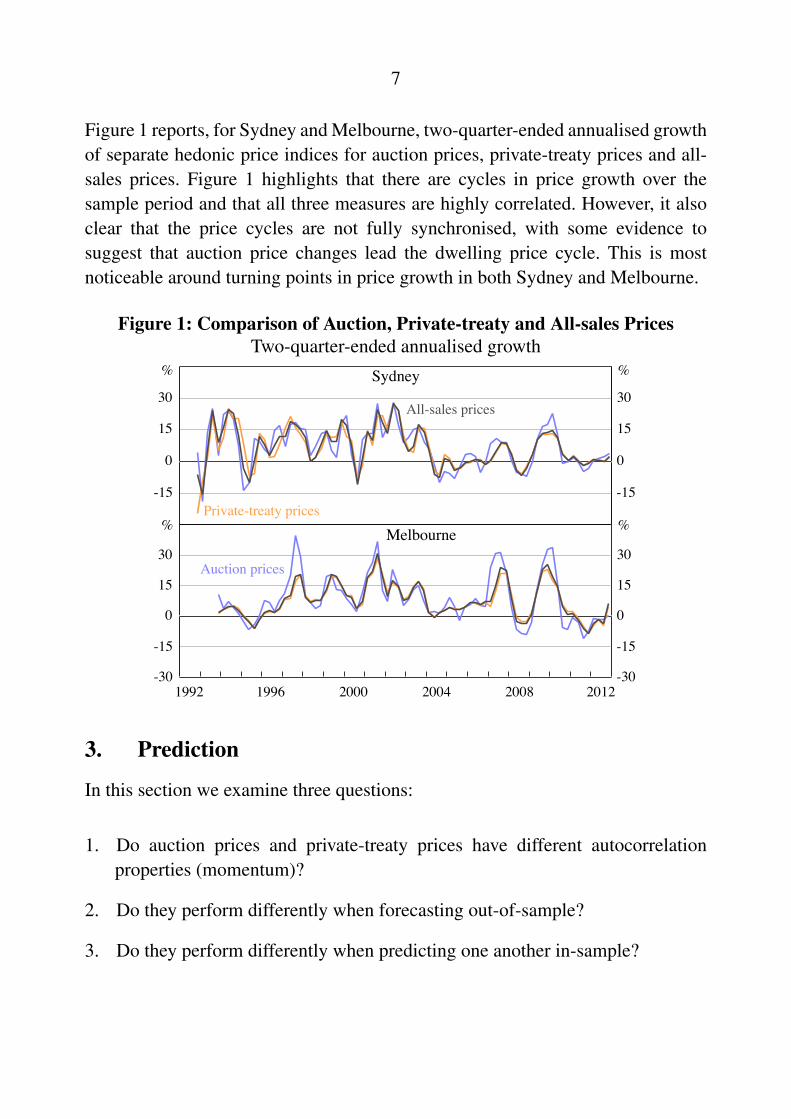
Figure 1 reports, for Sydney and Melbourne, two-quarter-ended annualised growthof separate hedonic price indices for auction prices, private-treaty prices and all-sales prices. Figure 1 highlights that there are cycles in price growth over thesample period and that all three measures are highly correlated. However, it alsoclear that the price cycles are not fully synchronised, with some evidence tosuggest that auction price changes lead the dwelling price cycle. This is mostnoticeable around turning points in price growth in both Sydney and Melbourne.

Figure 1: Comparison of Auction, Private-treaty and All-sales PricesTwo-quarter-ended annualised growth

2012

Melbourne

%Sydney

-15

0

15

30

-15

0

15

30

-30

-15

0

15

30

-30

-15

0

15

30

20082004200019961992

%

%%

All-sales prices

Private-treaty prices

Auction prices

3. Prediction

In this section we examine three questions:

1. Do auction prices and private-treaty prices have different autocorrelationproperties (momentum)?

2. Do they perform differently when forecasting out-of-sample?

3. Do they perform differently when predicting one another in-sample?

8

Answering the first question speaks to the well-established literature on theefficiency of housing markets, which suggests that dwelling prices are positivelyautocorrelated, as discussed in Case and Shiller (1989), Cutler, Poterba andSummers (1991), Cho (1996) and Capozza, Hendershott and Mack (2004) amongothers. Differences in momentum can also provide insight into the ability of thedata to discriminate between alternative theoretical models of the autocorrelationin buyers’ and sellers’ valuations (this is discussed further in Section 5). Thesecond question addresses whether any gains in predictive content can be usefulin real time and considers forecasting growth in a measure of average prices usingall sales.

We also consider in-sample analysis, the third question, for three reasons. First, itis possible that revisions to the estimated price indices for either auction or private-treaty prices could affect out-of-sample forecasting performance. By focusing onthe full sample of data we are able to abstract from the effects of revisions to theestimated price indices.

Second, in-sample analysis allows us to relax some of the assumptions maintainedin the out-of-sample analysis. In particular, using in-sample techniques we cancompare the ability of the two series to predict each other without necessarilyassuming a vector error correction model (VECM) representation with finitelags.8 Third, it has been argued that out-of-sample analysis can imply a loss ofinformation and power relative to in-sample analysis (see, for example, Inoue andKilian (2005)).

3.1 Momentum

Focusing first on the differences in autocorrelation properties, autocorrelationfunctions show that growth of average prices (all-sales price growth) is positivelyautocorrelated for up to one year, but that the strongest correlations are for thefirst two lags of quarterly growth (Figure 2). Considering the autocorrelationfunctions by sale mechanism highlights that all of the positive autocorrelation

8 Although a VECM with finite lags is a natural framework for modelling prices given that theyare likely to share the same common trend, it is not an immediate implication of theory andso we build up a case to support this representation, rather than simply assume it is valid (seeAppendices B and C).

9

in aggregate price growth for Sydney arises from the autocorrelation in private-treaty price growth; there is no evidence to suggest that auction price growth ispositively autocorrelated. Indeed, auction prices follow a random walk with drift.This is a quite striking result and suggests that all available information concerningdwelling prices is fully incorporated into auction prices within a quarter, which isconsistent with a weak version of the efficient market hypothesis.9

Figure 2: Autocorrelation Functions for Prices Growth

2 4 6 8 10 12 14 16-0.25

-0.13

0.00

0.13

0.25

0.38

Melbourne

2 4 6 8 10 12 14 16-0.25

-0.13

0.00

0.13

0.25

0.38

Sydney

n Auction pricesn Private-treaty pricesn All-sales prices

Quarters

**

*****

Note: Columns with asterisks denote significance at the 5 per cent level when using Bartlett’sMA(q) formula.

For Melbourne, most of the autocorrelation in all-sales price growth is alsodriven by autocorrelation in private-treaty price growth, although there issome evidence of first-order autocorrelation in auction price growth. Thedifference in autocorrelation functions, with private-treaty price growth beingmore autocorrelated than auction price growth, will subsequently be useful fordetermining whether buyer or seller valuations are autocorrelated, as discussedfurther in Section 5.

9 See, for example, Cho (1996).

10

3.2 Out-of-sample

We now consider whether measures of average prices, separated according to thetype of sale, are useful for predicting all-sales price growth out-of-sample and inreal time. Specifically, we consider whether the inclusion of either lagged auctionprices or lagged private-treaty prices can improve upon the one-quarter-aheadforecasts of all-sales price growth when using a single equation autoregressivemodel. To do this, we compare the following three forecasting models:10

∆st = µs +J∑

j=1

φ j∆st− j + εst (1)

∆st = µs +Γsst−1 +Γaat−1 +J∑

j=1

φ j∆st− j +

J∑j=1

γaj ∆at− j + ε

s,at (2)

∆st = µs +Γsst−1 +Γppt−1 +

J∑j=1

φ j∆st− j +

J∑j=1

γpj ∆pt− j + ε

s,pt (3)

where st is the average dwelling price based on all sales, at is the average auctionprice and pt is the average private-treaty price (all measured in logs). Equation (1)is the benchmark model, a univariate autoregression in average all-sales pricegrowth. Equation (2) nests the same autoregression, but also includes lags inauction prices. It also allows for all-sales and auction prices to be cointegrated,consistent with the idea that these price measures share the same common trend.Equation (3) incorporates lags of private-treaty prices instead of lags of auctionprices and also allows for cointegration.

We define:σ

2i ≡ E

(sit+1|t− st|t−

(st+1|t+1− st|t+1

))2

for i = 1,2,3 as the respective mean-squared prediction errors (MSPEs) for one-quarter-ahead all-sales price growth associated with Equations (1), (2) and (3)

10 In these, and all subsequent out-of-sample forecasting tests, we use four lags when usingSydney data and three lags when using Melbourne data. This is based on likelihood-ratioand residual serial correlation tests, as well as information criteria (see Appendix A). ForMelbourne, quarterly seasonal dummies are included as additional control variables, consistentwith evidence of seasonality in Melbourne.

11

respectively. sit+1|t ≡ E

(sit+1 | It

)is the one-quarter-ahead forecast of the log

all-sales price level based on Equation i (for i = 1,2,3) and using all availableinformation up to time t. st|τ is the measured value of the log all-sales price levelat time t given all available information up to time τ ≥ t. We consider whether theMSPEs are statistically different between Equations (1), (2) and (3) using pairwisecomparisons and the MSE-t test statistic discussed in McCracken (2007).11

The results in Table 2 suggest that Equation (2) can outperform the benchmarkmodel – that is, there is information content in lagged auction prices. In both cities,the MSPEs for Equation (2) are significantly lower relative to the benchmarkmodel in the order of 10 and 18 per cent for Sydney and Melbourne (column one,rows one and three). In contrast, there is no evidence to suggest that private-treatyprices can also improve upon forecasts relative to the benchmark model; the nullthat the forecast accuracy of Equation (3) is the same as that of the benchmarkcannot be rejected at conventional significance levels (column one, rows two andfour).

Table 2: Pairwise Nested Model MSPE Comparisonσ

2y∈{a,p}

σ2s

MSE-t statistic

SydneyH0 : σ

2s −σ

2a = 0 0.90** 0.85

H0 : σ2s −σ

2p = 0 0.93 0.26

MelbourneH0 : σ

2s −σ

2a = 0 0.82** 1.46

H0 : σ2s −σ

2p = 0 0.97 0.17

Notes: The alternative hypothesis for each test is that the MSPE of the restricted model, σ2s , is greater than the

unrestricted alternative (either σ2a or σ

2p ); recursive estimation is used starting with the sample period from

March 1992 to March 2007 for Sydney and from March 1993 to September 2008 for Melbourne; ***, **and * denote significance at the 1, 5 and 10 per cent levels respectively

11 The MSE-t statistic we compute is equivalent to the S1 test statistic proposed by Diebold andMariano (1995). It uses a mean-squared loss criterion, allows for contemporaneous and seriallycorrelated prediction errors, and is computed under the null that the difference in the mean-squared prediction errors (one-quarter-ahead) for two alternative forecasting equations is zero.As noted in McCracken (2007), when working with nested prediction equations the MSE-t teststatistic may not be well approximated by a normal distribution, and so we use the alternativecritical values tabulated in the same paper. Qualitatively similar results are obtained using theMSPE-adj t statistic suggested in Clark and West (2007).

12

To further establish whether it is in fact auction prices or private-treaty prices thatcontain predictive information for future price growth, we consider whether theseprice measures are useful in predicting one another. Specifically, we use out-of-sample Granger causality tests assuming that auction and private-treaty prices arecointegrated.

The unrestricted model used for our tests is given by:

∆at = µa +αa(at−1−β pt−1

)+

J∑j=1

Γaaj ∆at− j +

J∑j=1

Γapj ∆pt− j + ε

at (4)

∆pt = µp +αp(at−1−β pt−1

)+

J∑j=1

Γpaj ∆at− j +

J∑j=1

Γppj ∆pt− j + ε

pt (5)

The null hypotheses are that auction prices do not Granger cause private-treatyprices, H0 : αp = Γ

paj = 0 for all j, and that private-treaty prices do not Granger

cause auction prices, H0 : αa = Γapj = 0 for all j. Testing these hypotheses using

the approaches suggested by McCracken (2007) and Clark and West (2007), theresults in Table 3 highlight that we can reject the null that auction prices do notGranger cause private-treaty prices, but fail to reject the null that private-treatyprices do not Granger cause auction prices in Sydney (and only find weak evidenceto reject the null in Melbourne). These results confirm that auction prices appearto be more useful when forecasting out-of-sample.

Table 3: Out-of-sample Granger Causality TestsSydney Melbourne

H0 : Auction prices do not Granger cause private-treaty pricesMcCracken: MSE-t 1.55*** 1.38**Clark and West: MSPE-adj t 2.82*** 2.34***H0 : Private-treaty prices do not Granger cause auction pricesMcCracken: MSE-t –1.06 0.63*Clark and West: MSPE-adj t 0.50 1.46*Notes: ***, ** and * denote significance at the 1, 5 and 10 per cent levels of significance respectively; McCracken:

MSE-t is the Diebold and Mariano test statistic used in the context of a nested model forecast comparisonas discussed in McCracken (2007); Clark and West: MSPE-adj t is an alternative test statistic proposedby Clark and West (2007); estimates and out-of-sample forecasts are generated recursively with the initialin-sample estimation period from March 1992 to September 2002 for Sydney, and from March 1993 toSeptember 2002 for Melbourne

13

3.3 In-sample

Although out-of-sample findings are informative for comparing forecastingperformance in real time, a limitation of the previous comparisons is that theycan imply a loss of information and power relative to in-sample predictioncomparisons (see, for example, Inoue and Kilian (2005)), and can be affected byrevisions.

To consider whether these issues are important, we undertake the previousbivariate causality tests in-sample using the testing procedure discussed in Todaand Yamamoto (1995) and Dolado and Lutkepohl (1996). One useful feature ofthis approach is that it only requires the order of integration of the data to becorrectly specified, as the test remains consistent irrespective of whether auctionand private-treaty prices are cointegrated or not.12

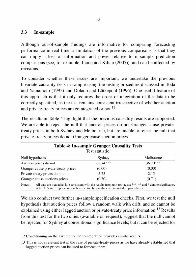
The results in Table 4 highlight that the previous causality results are supported.We are able to reject the null that auction prices do not Granger cause private-treaty prices in both Sydney and Melbourne, but are unable to reject the null thatprivate-treaty prices do not Granger cause auction prices.

Table 4: In-sample Granger Causality TestsTest statistic

Null hypothesis Sydney MelbourneAuction prices do not 68.74*** 36.70***Granger cause private-treaty prices (0.00) (0.00)Private-treaty prices do not 5.75 2.15Granger cause auctions prices (0.30) (0.71)Notes: All data are treated as I(1) consistent with the results from unit root tests; ***, ** and * denote significance

at the 1, 5 and 10 per cent levels respectively; p-values are reported in parentheses

We also conduct two further in-sample specification checks. First, we test the nullhypothesis that auction prices follow a random walk with drift, and so cannot beexplained using either lagged auction or private-treaty price information.13 Resultsfrom this test for the two cities (available on request), suggest that the null cannotbe rejected for Sydney at conventional significance levels; but it can be rejected for

12 Conditioning on the assumption of cointegration provides similar results.

13 This is not a relevant test in the case of private-treaty prices as we have already established thatlagged auction prices can be used to forecast them.

14

Melbourne, as lagged auction prices do appear to contain some predictive contentfor that city.

In the second, we check whether auction and private-treaty prices share the samecommon trend in prices and are, therefore, cointegrated as assumed in the previousout-of-sample analysis. Evidence in favour of cointegration, using the full sampleof data, is reported in Appendix A. Estimates of the cointegrating vectors andadjustment parameters are reported in Table 5. Consistent with our previousfindings, the results highlight that private-treaty prices respond to past deviationsbetween auction and private-treaty prices as the adjustment parameters on thelagged cointegrating relationship – αp in Equation (5) – are significant in bothSydney and Melbourne (column two). In contrast, auction prices do not respondto the same deviation as the adjustment parameters – αa in Equation (4) – areinsignificant in both cities (column one). The cointegration parameter, β for eachcity, also looks reasonable and not too far from 1, as one might expect.14

Table 5: Cointegration and Adjustment Parameter EstimatesAuction prices Private-treaty prices

SydneyCointegration parameter 1 1.05***

(.) (0.01)Adjustment parameter –0.10 0.42***

(0.23) (0.15)MelbourneCointegration parameter 1 1.08***

(.) (0.01)Adjustment parameter –0.02 0.18**

(0.14) (0.07)Notes: Cointegration and adjustment parameter estimates are obtained using Johansen MLE and normalising the

coefficient on auction prices to 1; ***, ** and * denote significance at the 1, 5 and 10 per cent levelsrespectively and are with respect to 0 for the adjustment parameters and 1 for the cointegration parameters;standard errors are reported in parentheses

In sum, the data are consistent with the following empirical facts:

1. Forecasts from an autoregression of all-sales prices can be significantlyimproved upon by including lagged auction price information. Lagged private-treaty prices are less informative.

14 Including additional characteristic controls for Melbourne and restricting the sample to beginfrom December 1997 leads to an estimated β of 1.05.

15

2. Auction prices Granger cause private-treaty prices, but private-treaty prices donot Granger cause auction prices. This holds both in- and out-of-sample.

3. The auction price level process is not statistically different from a randomwalk with drift in Sydney. There is some evidence that the first lag of auctionprice growth can be used to forecast auction price growth in Melbourne.

4. Auction and private-treaty prices are cointegrated.

4. The Persistence of Shocks

We now consider whether alternative measures of average prices, based on the typeof sale, can provide information about the persistence of shocks to dwelling prices.To answer this question, we use two conditions supported in the data: (a) thatauction and private-treaty prices are cointegrated and can be represented by aVECM ; and (b) that private-treaty prices do not Granger cause auction prices.That is:

∆at = µa +

J∑j=1

Γaaj ∆at− j + ε

at (6)

∆pt = µp +αp(at−1−β pt−1

)+

J∑j=1

Γpaj ∆at− j +

J∑j=1

Γppj ∆pt− j + ε

pt (7)

Together, these conditions are sufficient for identifying the effects of permanentand transitory shocks to auction and private-treaty prices.15 A permanent shockis defined as having an effect on long-run forecasts of auction and private-treatyprices whereas a transitory shock has no such effects.

Table 6 reports forecast error variance decompositions for Sydney and Melbourneof the permanent and transitory shocks assuming that both conditions hold.We only report the decomposition for private-treaty prices, as conditions (a) and(b) together necessarily imply that variation in auction prices can only be attributedto permanent shocks. Relaxing assumption (b) and assuming that only the long-run

15 For further discussion on this point, see Fisher and Huh (2007) and Pagan and Pesaran (2008).

16

adjustment parameter in the auction price equation is zero16 leads to very similarresults.

Table 6 highlights that almost half of the forecast error variation in private-treatyprices one-quarter-ahead is due to transitory shocks. At the two-quarter- and four-quarter-ahead horizons, transitory shocks account for about 20 and 10 per cent ofthe forecast error variances respectively.

Table 6: Forecast Error Variance Decompositions for Private-treaty PricesForecast Sydney Melbournehorizon Permanent Transitory Permanent Transitory1 0.45 0.55 0.53 0.472 0.77 0.23 0.81 0.193 0.82 0.18 0.87 0.134 0.89 0.11 0.91 0.0932 0.99 0.01 0.99 0.01

Figure 3 graphs estimates of the permanent and transitory shocks over time. Wesee very clearly that the estimated permanent shocks are much larger than theestimated transitory shocks. In particular, the period covering the mid 1990s to the2000s is a period in which permanent shocks were having a noticeable positiveeffect on dwelling price growth. This is consistent with the typical explanationsfor changes in dwelling prices during this period, including the effects of financialderegulation and productivity improvements, and a shift to easier access to creditand lower real interest rates.17

In contrast, the transitory shocks to auction and private-treaty prices are smaller inmagnitude. The most prominent periods of positive transitory shocks were in therecovery from the early 1990s recession and around 2001 to 2003. Even duringthe global financial crisis, the estimates suggest that there were no large transitoryshocks to dwelling prices. This is interesting given that for other countries thecrisis has generally been interpreted as a demand shock, and the conventionalwisdom is that demand shocks have only transitory effects on dwelling prices.

16 That is, if we only impose the restriction that αa = 0 rather than αa = Γapj = 0 for all j = 1, ...,J

with respect to Equation (4).

17 See, for example, Ellis (2006) and Yates (2011).

17

Figure 3: Estimates of Permanent and Transitory Shocks

-0.05

0.00

0.05

-0.05

0.00

0.05

-0.10

-0.05

0.00

0.05

-0.10

-0.05

0.00

0.05

2012

Sydney

%Permanent shocks

Transitory shocks

Melbourne

%

%%

2008200420001996

Two key properties of the propagation of permanent and transitory shocks arehighlighted by the impulse response to a one standard deviation permanent shock,and a one standard deviation transitory shock respectively (Figure 4). The firstis that auction prices adjust more quickly than private-treaty prices in responseto a permanent price shock. Calculating the fraction of the long-run increase inprices (limh→∞ Et

(yt+h

)for yt = at , pt) that has occurred in a given period, we

see that around 80 (Sydney) to 60 (Melbourne) per cent of the long-run increasein prices occurs within the first quarter for auction prices, but only around 35 to25 per cent of the adjustment has occurred for private-treaty prices. After fourquarters, roughly 95 per cent of the adjustment to the long-run auction price hasoccurred for both Sydney and Melbourne. In contrast, when using private-treatyprices approximately 85 to 75 per cent of the adjustment to their long-run pricelevel has been completed after four quarters.

18

Figure 4: Impulse Response Functions to a One Standard Deviation ShockSy

dney

Quarters2 4 6 8 10 12 14 16

-1.8

0.0

1.8

3.6

5.4

2 4 6 8 10 12 14 16-1.8

0.0

1.8

3.6

5.4

0.0

1.8

3.6

5.4

0.0

1.8

3.6

5.4

Mel

bour

ne

Auction prices

Private-treaty prices

%

%

%

%Permanent shock Transitory shock

Notes: Impulse response functions to a one standard deviation shock estimated under theassumption that auction and private-treaty prices admit a VECM and that private-treatyprices do not Granger cause auction prices; confidence intervals are at the 95 per centlevel of significance and are bootstrapped using Hall’s percentile method

The second property to note is that transitory price shocks have smaller effectson private-treaty prices than do permanent shocks. The restrictions supportedby our previous empirical findings – that auction and private-treaty prices canbe represented by a VECM and that private-treaty prices do not Granger causeauction prices – imply that transitory shocks have no effect on auction prices.

5. Why Does the Mechanism of Sale Matter?

This section shows how the micro structure of the different trade mechanisms,and the nature of shocks to agents’ valuations, can provide an interpretation of ourprevious empirical findings. The first step is to justify our assertion that, relative toprivate-treaty prices, prices at auctions are more responsive to shocks to buyers’

19

valuations than they are to sellers’ valuations (Section 5.1). The second step isto rationalise why buyers’ valuations respond to new information about dwellingprices more quickly than sellers’ valuations (Section 5.2). The third is to bringthese two results together to explain our previous empirical findings (Section 5.3).

5.1 Some Intuition for the Theory

We begin by considering the simplest trade mechanisms: an ascending open-bid(or English) auction (the mechanism most commonly used in Australia), withouta seller reserve price, to model auctions; and a Nash bargaining solution tomodel sales that use bilateral private-treaty negotiations. In the English auction,the price rises until no bidder (hereafter buyer) is willing to offer more. In theNash bargaining solution, the price is a weighted average of the buyer and sellervaluation. To further simplify, we assume that buyers at auctions have privatevalues,18 and that any buyer values the dwelling more than any seller. That is,the dwelling is always sold through either mechanism. These assumptions areunrealistic, but they are useful to provide the basic intuition. They are relaxedin a formal analysis below.

It is a dominant strategy for a buyer to bid until the point at which his or her privatevaluation is reached, and then exit the auction.19 Thus, bidding continues until thebuyer with the second-highest valuation exits the auction, leaving only the buyerwith the highest valuation who wins the auction and pays a price equal to thesecond-highest valuation. An implication of this model is that a common shockto all buyers’ valuations will increase the auction price one for one. Furthermore,since there is no seller reserve, sellers’ valuations have no effect on the equilibriumauction price.

In a private-treaty negotiation with Nash bargaining, a shock to the buyer’svaluation will only partially increase the price, since the negotiated price is a

18 That is, knowledge of other buyers’ valuations has no impact on any given buyer’s valuation.19 To see why, suppose a seller exited before the price reached their valuation. In this case, there

is a positive probability that the buyer could have remained in the auction and paid a price lessthan their valuation. The buyer has thus forgone a profitable trading opportunity and so thiscannot be an equilibrium strategy. Conversely, suppose the buyer remained in the auction whenthe price is above their valuation. In this case, there is a positive probability the buyer wins andpays a price that is higher than their valuation, thus engaging in trade that is not profitable tothem. This also cannot be an equilibrium strategy.

20

weighted average of the buyer’s and seller’s valuation. In particular, the price willonly go up by the weight on the buyer’s valuation, which under Nash bargaining,reflects the relative bargaining strength of the seller.20 In a market where buyersand sellers have equal bargaining power, prices will be equally responsive to acommon shock to buyers’ valuations as they are to a common shock to sellers’valuations. Only if sellers have all the bargaining power will private-treaty pricesbehave like auction prices, responding only to buyer shocks and not seller shocks.

The assumptions we have maintained so far, that all auctions and bilateralnegotiations end in a sale and that buyers have private values, are useful in makingour general point, but they are restrictive. We relax them below.

5.1.1 When not all auctions or negotiations end in a sale

When not all auctions end in a sale, sellers’ valuations will matter. To incorporatethis phenomenon in our theoretical analysis, we consider the reserve price, whichis a minimum price demanded by the seller. In auctions in NSW and Victoria, avendor bid, which is a bid made by the auctioneer on behalf of the seller, can beused to effect a reserve price that conditions on the information revealed throughthe auction.21 Alternatively, the seller can simply choose not to sell the property ifbidding does not exceed their reserve price.22

The first implication of the seller using a reserve price R is that not all auctionsend in a transaction: when R is above the valuation of the highest buyer thedwelling does not sell. R can affect the value of the winning bid: when R is belowthe valuation of the highest buyer, but higher than the second-highest buyer’svaluation, the dwelling sells at the price R. Only when R is below the second-highest buyer’s valuation does the reserve price have no effect on the auctionoutcome or the price obtained.

20 Recall that with a Nash bargain, a stronger seller position implies a transaction price that iscloser to the buyer’s valuation (and so more of the surplus from trade accrues to the seller).

21 This is different from a reserve price set prior to the auction. Even if a reserve price is setprior to auction, the ability to make a vendor bid implies that the seller can effectively revisetheir reserve price, conditioning on information revealed through the auction. In the privatevalues case, the optimal pre-announced reserve price and vendor bid are equivalent. Vendorbids are permissible in both Sydney and Melbourne – see, for example, Consumer AffairsVictoria (2014) and NSW Fair Trading (2014).

22 Again, refer to Consumer Affairs Victoria (2014) and NSW Fair Trading (2014).

21

Consider now the effect on the auction price of an increase in R. When the auctionends without a sale, an increase in R has no effect on the auction outcome or theabsence of price due to the fact the dwelling is passed in. When the auction issuccessful, there are three possible cases: one, an increase in R does not crossthe threshold of the second-highest buyer’s valuation and so has no effect on theequilibrium price; two, it does cross the threshold, in which case an increase inR will affect prices but less than one for one (by the amount by which R exceedsthe second-highest valuation); and three, R is initially above the second-highestvaluation and is raised, increasing prices one for one. If R becomes too high,however, crossing the valuation threshold for the buyer with the highest valuation,the auction is passed in and excluded from the dwelling price transactions data.

Thus R plays one of two roles, if any, at a given auction: either an increase in Rweakly increases the winning bid to the seller, with the magnitude depending uponthe initial and final values of R in relation to the highest and second-highest buyervaluations; or it prevents a trade that would otherwise occur from taking place. Thelatter is a selection effect and leads to higher prices in the observed transactionsdata. The total effect of a change in R on the average auction price is the weightedaverage of these two effects.

Our interest is in how shocks to sellers’ valuations affect the average auctionprice in this more complicated environment. The effect operates solely throughthe reserve price. Thus, the effect of a common shock to sellers’ valuations isthe composition of the effect of the shock on reserve prices and the effect ofthe reserve price on the transaction price. Assuming that the seller chooses thereserve price optimally – that is, with the goal of maximising the expected auctionprice – we can determine the overall effect conditioning on the distribution ofbuyers’ valuations and that of sellers. When both are uniform, and there are morethan three buyers, then the effect of a seller shock on average price is an order ofmagnitude less than that of a buyer shock. This conclusion holds more generallyamong (weakly) left-skewed distributions that belong to the generalized Paretodistribution family, and which nests the uniform distribution.

The arguments for private-treaties with Nash bargaining are quite different.In private-treaties, an increase in all sellers’ valuations will increase prices intransactions that remain profitable to the buyer and the seller by the amount of thebuyer’s bargaining weight. This also results in a selection effect, removing from

22

the transactions data those dwellings where the seller now values the dwellingmore than the buyer they meet. What we show below is that if the dispersion ofbuyers’ and sellers’ valuations are constant, then the selection effect is again lessimportant for changes in private-treaty prices. What is of primary importance isthe sensitivity of prices to average buyers’ and sellers’ valuations, as reflected inthe relative bargaining strengths of the two groups. Unless there is a special reasonto believe that sellers have all of the power in dwelling transaction negotiations,in all states of the dwelling price cycle, it is difficult to move away from theinterpretation that both buyers and sellers are important in changes in private-treaty prices.

5.2 Differences in the Response to New Information

The previous intuition argues that changes in auction prices mainly reflect changesin buyers’ valuations, whereas changes in private-treaty prices reflect changesin both buyers’ and sellers’ valuations. If we extend this argument, and assumethat buyers’ valuations respond more quickly to news relevant to dwelling pricesthan do sellers’, these two facts can explain the previous empirical findings: thatauction price growth is not highly autocorrelated but private-treaty price growthis; that auctions are more useful for forecasting; and that auctions better reflect thecommon trend in all prices.

In particular, if there is a shock to the common stochastic trend in all prices(which is a permanent shock), and all buyers update their valuations quickly,then auction prices must be indicative of the common trend and respond quitequickly to permanent shocks as highlighted in Figure 3. Conversely, if sellersupdate their valuations more slowly, private-treaty prices will still be indicativeof the common trend (prices are cointegrated), but will also measure transitorydepartures from this trend. This can explain why private-treaty price growth ismore autocorrelated than auction price growth (because the transitory componentinduces autocorrelation); why auction prices are more useful for forecasting(because they quickly capture changes in the common trend, whereas it takes moretime for private-treaty prices to fully update to this trend); and why auction pricesare a better measure of the underlying common stochastic trend – because they arenot perturbed by transitory shocks that are specific to sellers’ valuations.

23

Theoretical explanations for why sellers respond more slowly include: equity lock-in (Stein 1995; Genesove and Mayer 1997); rigidity of seller reservation pricesdue to reference point pricing, whether with respect to the seller’s purchase price(Genesove and Mayer 2001) or original list price; and differential non-centralisedinformation flows (Carrillo 2012; Genesove and Han 2012). We now consider themore formal analysis that underpins the previous intuition.

5.3 A More Formal Treatment

We consider two simple models of price determination; an affiliated values Englishauction and a Nash bargain for bilateral (private-treaty) negotiations. These twomodels are plausible characterisations of the Australian property market. A formaldescription of the two models is outlined in Appendix B.

5.3.1 Auction prices

Focusing first on auctions, we assume that in each quarter there are manyEnglish auctions – the auction mechanism most commonly used in the Australianhousing market. In any one auction, bids are observed by all other buyers andthe buyer with the highest bid wins, paying that amount. We assume that buyersare risk neutral and have valuations that are linear and affiliated (Milgrom andWeber 1982; Klemperer 1999) as follows:23

vait = ψats

ait +

γatnat−1

∑j 6=i

sajt

sait = µ

Pt + ε

ait

The valuation of buyer i in auction a held at time t is given by vait and sa

it is buyer i’ssignal (or estimate) of the value of the dwelling. Importantly, the above modellingdevice assumes that buyer valuations are a function of their own signal and otherbuyer’s signals (in the same auction). As bids are announced during an auction,buyers update their valuations to reflect the information contained in other buyers’bids.

23 Although the results we derive below are conditioned on the assumption of risk neutrality, thisassumption can be relaxed if common values – a specific case of affiliation – are assumed.

24

For example, if there are many buyers who participate in auction a at time tand continue to make bids as the price in that auction rises, then this providesinformation to other active buyers – namely that many other buyers must havehigh estimates of that dwelling’s value. Each buyer then infers that it is more likelythat the true value of dwelling a at time t is high, and revises their own valuationupwards.

What stops the process is that buyers only update their signal partially in responseto the information contained in others’ bids (by the weighting γat

nat−1). When theprice becomes sufficiently high, buyers start to exit the auction (stop makingbids), which is observed by other participants. This continues until there is asingle buyer remaining, at which point the auction concludes and the dwellingis sold.24 Although we have abstracted from the effects of a seller reserve price,the underlying intuition remains similar.25

We assume that each signal comprises a common component µPt (the common

stochastic trend) and an idiosyncratic component εait , where the latter is drawn

from a uniform distribution on the bounded interval [−θat ,θat ]. The weights ψatand γat can be interpreted as the weights attached to a buyers’ own signal and themean signal of other buyers in the auction respectively.

The assumption of linear affiliation,26 in conjunction with symmetric biddingstrategies and an English auction, implies that the sale price for a successfulauction will, in general, be a function of all buyers’ signals. For this reason,information is both revealed and aggregated into the price during the auction.It should be noted that the type of affiliation we have modelled can be used to

24 Another way to think of our modelling device is that all players in the auction hold a biddingcard which remains raised until the price quoted hits the maximum that that buyer is willingto bid, at which point they lower the card and exit the auction, and all other players observethis. Importantly, with affiliation, the maximal bid for any given buyer is a function of both thenumber of buyers who have already exited the auction and the price point at which each buyerstopped participating.

25 It also does not materially affect the analysis that follows (see Appendix D).26 Intuitively, affiliation of buyers’ values implies that there is correlation between values. For

example, with two buyers, affiliation implies that an increase in the valuation of buyer 1 alsoincreases the likelihood that buyer 2 holds a higher valuation. The converse is also true: anincrease in buyer 2’s valuation increases the likelihood that buyer 1 has a higher valuation.Affiliation is a stronger concept than correlation, as it requires local positive correlationeverywhere with respect to the joint distribution of valuations (see Klemperer (1999)).

25

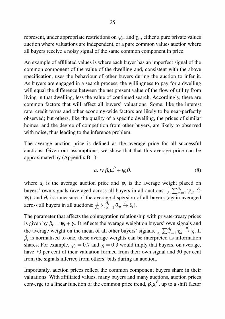
represent, under appropriate restrictions on ψat and γat , either a pure private valuesauction where valuations are independent, or a pure common values auction whereall buyers receive a noisy signal of the same common component in price.

An example of affiliated values is where each buyer has an imperfect signal of thecommon component of the value of the dwelling and, consistent with the abovespecification, uses the behaviour of other buyers during the auction to infer it.As buyers are engaged in a search process, the willingness to pay for a dwellingwill equal the difference between the net present value of the flow of utility fromliving in that dwelling, less the value of continued search. Accordingly, there arecommon factors that will affect all buyers’ valuations. Some, like the interestrate, credit terms and other economy-wide factors are likely to be near-perfectlyobserved; but others, like the quality of a specific dwelling, the prices of similarhomes, and the degree of competition from other buyers, are likely to observedwith noise, thus leading to the inference problem.

The average auction price is defined as the average price for all successfulauctions. Given our assumptions, we show that that this average price can beapproximated by (Appendix B.1):

at ≈ βt µPt +ψtθt (8)

where at is the average auction price and ψt is the average weight placed onbuyers’ own signals (averaged across all buyers in all auctions: 1

At

∑Atat=1 ψat

p→ψt), and θt is a measure of the average dispersion of all buyers (again averagedacross all buyers in all auctions: 1

At

∑Atat=1 θat

p→ θt).

The parameter that affects the cointegration relationship with private-treaty pricesis given by βt = ψt + γt . It reflects the average weight on buyers’ own signals andthe average weight on the mean of all other buyers’ signals, 1

At

∑Atat=1 γat

p→ γt . Ifβt is normalised to one, these average weights can be interpreted as informationshares. For example, ψt = 0.7 and γt = 0.3 would imply that buyers, on average,have 70 per cent of their valuation formed from their own signal and 30 per centfrom the signals inferred from others’ bids during an auction.

Importantly, auction prices reflect the common component buyers share in theirvaluations. With affiliated values, many buyers and many auctions, auction pricesconverge to a linear function of the common price trend, βt µ

Pt , up to a shift factor

26

of ψtθt . The latter term comprises the average weight that buyers assign to theirown signal, and the average dispersion of buyers’ valuations. Thus, for auctions,an increase in the weight that buyers assign to their own signal or an increase in thedispersion of buyers’ valuations could, in principle, lead to temporary deviationsof auction prices from the common price trend.

Greater dispersion in buyers’ valuations will tend to raise the average pricebecause it is the indifference condition for the second-last buyer remaining (i.e. thepoint at which the buyer with the second-highest valuation drops out) that isimportant for determining the final price. With a large number of buyers, greaterdispersion in buyers’ valuations will not affect the inferred common componentof signals from buyers who have already exited the auction, but it will raise theprobability that the buyers with the highest and second-highest valuations willhave high valuations and so a higher price will be more likely. Accordingly, ahigher average auction price could reflect an increase in average buyer dispersion,rather than an increase in the common trend in prices.

Similarly, an increase in the weight that buyers assign to their own signal couldalso drive a temporary increase in auction prices. Again, this relates to the fact thatprices are determined by the indifference condition for the buyer with the second-highest valuation. This buyer, like all buyers, weights their own signal differentlyto the weight placed on other buyers’ signals.27 In particular, when there are manybuyers, the importance of any one buyer (including the buyer with the highestsignal) on the mean signal is equal and small. In contrast, the weight the buyerwith the second-highest valuation places on their own signal is more important:changes in this weight can lead to transitory changes in auction prices, even whenaveraged across a large number of transactions.

27 At the price at which the buyer with second-highest valuation is indifferent between quittingor remaining in the auction, this buyer is comparing their own signal (with weight ψat) withthe likely signal of the other buyer who has not yet quit (with weight γat

nat−1 ). The fact that theweight on the second-last buyer’s own signal is potentially different from the weight on theother buyer’s signal (which is the same as for all other buyers who already exited the auction)means that it is the own-signal weight that becomes pivotal in price determination. For thisreason, a transitory change in the information weights, towards a greater weight on idiosyncraticinformation and a lower weight on other buyers’ information, could have a transitory effect onauction prices.

27

To understand these results in the context of the intuition given in Section 5.1,we have shown that under more general assumptions about buyers’ information,and when there are many buyers in each auction, the argument for the claim thatauctions are relatively more responsive to buyers’ than sellers’ valuations, whencompared with private-treaty sales, is similar to the private values case. Includingoptimal seller reserve prices, set by the seller after he or she has observed thewinning bid and therefore on the basis of the information revealed during theauction (Lopomo 2001), introduces a role for the seller’s valuation. However, heretoo, as in the private values case, the responsiveness of average auction pricesto a common shock in sellers’ valuations is substantially less than to a commonshock in buyer valuations. This is true given a sufficient number of buyers andin the baseline uniform distributions case, and with more general left-skeweddistributions of buyers’ valuations.

5.3.2 Private-treaty prices

For private-treaty prices, we assume that the price is the result of a Nash bargainbetween one buyer and one seller. That is, the surplus from trade (the differencebetween the buyer’s and the seller’s reservation values) is split between the buyerand seller according to their relative bargaining power. Again, we assume thatbuyers and sellers have a common stochastic trend and an idiosyncratic componentin their valuations:

vpsit = µ

Pt + ε

psit

vpbit = µ

Pt + ε

pbit

where the prospective seller’s idiosyncratic signal, εpsit , is drawn randomly from a

uniform distribution on [−φit ,φit ] and the prospective buyer’s idiosyncratic signal,ε

pbit , is drawn randomly from a uniform distribution on [−θit ,θit ]. For a sale to

occur, the idiosyncratic signal for the buyer must be weakly higher than that forthe seller, ε

pbit ≥ ε

psit . The average measured private-treaty price is the average

price of all successful private-treaty sales within a quarter. It can be approximatedby (see Appendix B.2):

pt ≈ µPt + f (ψt ,φt ,θt) (9)

The transitory or idiosyncratic components of buyers’ and sellers’ valuations aregiven by the function f , which has the Nash bargaining weight (ψt), the dispersion

28

of sellers (φt) and the dispersion of buyers (θt) in its arguments. We assume that thefunction f (ψt ,φt ,θt) can be approximated by a stationary autoregressive movingaverage (ARMA) process to be consistent with the autocorrelation in private-treatyprice growth observed in the data (Section 3.1).

The reason that the function f is not zero, even when averaging across a large setof transactions, is that prices only reflect successful negotiations. This implies thatbuyer and seller valuations are correlated (with all buyer valuations weakly higherthan that of the respective seller) and so idiosyncratic factors do not wash out onaverage.

The valuation of the common component of prices is identical for buyers andsellers and is assumed not to be predictable: µ

Pt = c+µ

Pt−1+η

Pt . We also make the

additional assumption that the average overall weight on information in auctions isconstant, βt = β . Under these assumptions, we can see that average auction prices,Equation (8), and average private-treaty prices, Equation (9), are cointegrated withcointegrating vector

[1 −β

]. To link these equations to our empirical findings,

Appendix C shows that Equations (8) and (9) can be approximated using theVECM:

∆at ≈ βc+βηPt (10)

∆pt ≈ c+α(at−1−β pt−1

)+

J∑j=1

γa j∆at− j +

J∑j=1

γp j∆pt− j +ηPt +ut (11)

This representation is valid provided we assume that average dispersion in buyers’valuations and the average weight that buyers place on their own information(averaged across all auctions in a given quarter) are constant. These assumptionsare sufficient for ensuring that changes in auction prices reflect changes in thecommon price trend, as found in our empirical analysis.

Importantly, the above VECM is fully consistent with our previous empiricalfindings. In particular, it implies that: growth in auction prices is notautocorrelated; that growth in private-treaty prices is autocorrelated; and thatauction prices will Granger cause private-treaty prices but that private-treaty priceswill not Granger cause auction prices.

29

There are four key implications to be drawn from the theoretical analysis. First,both auction prices and private-treaty prices measure the common trend in allprices, µ

Pt , when averaging across a large set of transactions. For this reason,

auctions are not necessarily more efficient at measuring the common trend in allprices.

Second, the different weighting of buyers’ and sellers’ valuations in different salesmechanisms appears to be important. Assuming our theoretical structure providesa reasonable approximation of actual price formation, our results imply that thereis a large set of distributions for which auction prices weight buyers’ valuationsmore highly than sellers’ valuations, when compared with private-treaty prices.If this is right, then it follows that the autocorrelation observed in private-treatyprices is more likely to be coming from the valuations of sellers.

Third, since private negotiation is intrinsic in the determination of private-treatyprices, the average dispersion of seller values and the relative bargaining strengthof buyers and sellers affect average private-treaty prices. These become plausiblesources of autocorrelation in private-treaty prices, but not auction prices.

Fourth, our theory is consistent with the idea that auction prices and private-treatyprices are cointegrated and measure the same common trend. As such, variationin either the average dispersion of sellers or relative bargaining strength can onlyinduce transitory variation in private-treaty prices and must, therefore, dissipatewith time.

6. Conclusion

This paper analyses whether the mechanism of sale is useful for forecastingaverage dwelling prices. Using hedonic price indices for Sydney and Melbourne,we show that auction prices and private-treaty prices have different statisticalproperties, including significant differences in their momentum, ability to forecasteach other, and ability to forecast average growth of prices overall.

Our results suggest that growth in auction prices is much less autocorrelated thangrowth in private-treaty prices – indeed, we could not reject the null of a randomwalk with drift in Sydney auction prices. This surprisingly strong result, whichholds even though the two measures share the same common price trend, suggeststhat auction prices incorporate new information more quickly than private-treaty

30

prices. Consistent with this, we find that including lagged information on auctionprices improves forecasts of average dwelling prices growth overall.

In addition, we find that auction prices Granger cause private-treaty prices, butthat the reverse is not true. When combined with the assumption that these twoprice series are cointegrated, this result is useful for separating prices into theirtransitory and permanent components and for forecasting the evolution of pricesat short-term forecasting horizons.

Empirically, we find that auction prices are driven by permanent shocks, whereasprivate-treaty prices are affected by both permanent and transitory shocks. Ifpermanent shocks are an accurate measure of changes in the common trend inall prices, as should be the case when there is cointegration, our results suggestthat auction prices are likely to be a better reflection of this common trend.Furthermore, the presence of transitory shocks in private-treaty prices implies thatthey take longer to incorporate changes in the common trend. This also helps toexplain why private-treaty prices are less useful when forecasting.

We interpret our empirical findings using two models of price formation – anEnglish auction with linearly affilated values and a bilateral Nash bargain. Weshow that these two models imply a VECM approximation that is consistent withour data. These two models of price formation, when combined with our empiricalfindings, suggest that the key issues at hand are: the extent to which the averagedispersion of valuations and the average bargaining strength of buyers and sellersaffect prices; whether the relative importance of buyers’ and sellers’ valuationsdiffers according to the mechanism of sale; and whether buyers and sellers behavedifferently in response to shocks.

The question we are interested in is whether distinguishing prices by themechanism of trade can assist in the forecasting of dwelling prices and inunderstanding the dwelling price cycle. On both empirical and theoretical grounds,we argue that the answer is yes. Separating prices by the type of sale, andmore specifically focusing on auction prices, can improve forecasting and inidentifying the persistence of shocks. We believe that these results are interestingboth narrowly, for those concerned with forecasting prices, and more broadly forunderstanding how price formation can provide alternative insights into dwellingprice cycles.

31

Appendix A: Specification Checks

To choose the appropriate number of lags in both the in- and out-of-sampleanalysis we use likelihood ratio tests, information criteria and tests for low-orderserial correlation in the VAR residuals (see Table A1). Taking these results intoconsideration, and the relative sample size, we use four lags for Sydney and threelags for Melbourne in our analysis (when working with data in its first-differenceor VECM representation).

Table A1: Lags Suggested According to Selection Criteria and ModelVAR in VAR in VAR in

auction and private-treaty and auction andall-sale prices all-sale prices private-treaty prices

SydneySequential LR tests(a) 7 5 1Akaike information criteria 7 2 1Sequential serial correlation tests(b) 7 7 7MelbourneSequential LR tests(a) 4 6 4Akaike information criteria 4 4 4Sequential serial correlation tests(b) 4 4 4Notes: (a) Denotes the number of lags suggested by applying sequential likelihood ratio (LR) tests (with a

maximum lag length of 8)(b) Denotes the number of lags by parring back the number of lags using sequential Lagrange-multipliertests; starting with a maximum lag length of 8, lags are sequentially dropped until the null hypotheses ofno low order (first or second) serial correlation is rejected at the 5 per cent level of significance

To test the order of integration of prices, Dickey-Fuller (DF) GLS regressions(Elliott, Rothenberg and Stock 1996; Ng and Perron 2001) are estimated (TableA2). Other tests for a unit root are also consistent with the prices data being I(1).

32

Table A2: Dickey-Fuller GLS RegressionsLags DF GLS τ 5 per cent

test statistic critical valueSydney auction pricesNg-Perron sequential t(a) 2 –0.97 –3.06Minimum Scharwz criteria(b) 1 –0.60 –3.08Minimum modified AIC(c) 2 –0.97 –3.06Sydney private-treaty pricesNg-Perron sequential t(a) 10 –1.54 –2.78Minimum Scharwz criteria(b) 1 –0.90 –3.08Minimum modified AIC(c) 1 –0.90 –3.08Melbourne auction pricesNg-Perron sequential t(a) 1 –2.04 –3.09Minimum Scharwz criteria(b) 1 –2.04 –3.09Minimum modified AIC(c) 1 –2.04 –3.09Melbourne private-treaty pricesNg-Perron sequential t(a) 6 –2.05 –2.93Minimum Scharwz criteria(b) 3 –1.82 –3.04Minimum modified AIC(c) 3 –1.82 –3.04Notes: (a) Lag length selected using Ng-Perron sequential t method as suggested by Ng and Perron (1995)

(b) Lag length selected using Scharwz criteria(c) Lag length selected using modified Akaike information criteria (AIC)

Table A3 suggests that auction and private treaty sales prices are cointegratedwhen using Johansen’s trace test. Evidence of cointegration is also foundat conventional significance levels assuming a known cointegrating vector,[

1 −1], and using univariate unit root tests such as augmented Dickey-Fuller

and Phillips-Perron tests (results are available on request).

Table A3: Cointegration Test ResultsH0: No cointegration H0: Single cointegrating vector

City Test statistic(a) Critical value(b) Test statistic(a) Critical value(b) LagsSydney 19.71 15.41 3.04 3.76 5Melbourne 16.21 15.41 1.42 3.76 4Notes: (a) Johansen’s trace test statistic

(b) The critical values reported are measured at the 5 per cent level of significance

33

Appendix B: A Theoretical Example

B.1 Auction Prices

For the auction price mechanism, we use a linear example of an affiliated valuesauction as discussed by Milgrom and Weber (1982) and Klemperer (1999). Weassume each time period (quarter) t that multiple English auctions occur. Eachauction (indexed by dwelling a at time t) has nat risk-neutral bidders (hereafterbuyers). Buyers’ valuations are given by:

vait = ψats

ait +

γatnat−1

∑j 6=i

sajt (B1)

where sait is buyer i’s private signal (estimate) of the worth of dwelling a in quarter

t, and ψat ≥ 0 is the weight attached to a buyer’s own signal and γat > 0 is theweight attached to the mean of other buyers’ signals.

We assume that each buyers’ own estimate of the worth of dwelling a in period tis given by a common component, µ

Pt , and an idiosyncratic component ε

ait :

sait = µ

Pt + ε

ait (B2)

We assume that εait is uniformly distributed with support [−θ

at ,θ

at ].

We assume buyers participate in an ascending bids English auction – themechanism commonly used to sell dwellings in Australia – and we abstract fromthe possibility that sellers can post a reserve price.28

28 See Appendix D for the inclusion of seller reserve prices.

34

A bidding strategy is given by the prices at which buyers are no longer willingto remain in the auction. The following bidding strategy is consistent with asymmetric equilibrium:

Bo(va

it)= (ψat + γat)va

it

B1

(snat :nat

,vait

)=

γatnat−1

sanat :nat

+

(ψat +

(nat−2)γatnat−1

)va

it

B2

(sa

nat :nat,sa

nat−1:nat,va

it

)=

γatnat−1

(sa

nat :nat+ sa

nat−1:nat

)+

(ψat +

(nat−3)γatnat−1

)va

it

...

Bnat−2

(sa

nat :nat, ...,sa

2:nat,va

it

)=

γatnat−1

nat∑j=3

saj:nat

+

(ψat +

γatnat−1

)va

it

where Bk(.,va

it)

represents the price at which a buyer with valuation vait drops out

given that k players have previously dropped out of the auction, and saj:nat

is the jthhighest signal of the value of dwelling a in period t (and so sa

1:nat> sa

2:nat> ... >

sanat :nat

). Note that in this equilibrium other buyers’ signals can be inferred as theyexit the auction. That is, information about the value of the dwelling is revealedthrough the auction process.

That this is a symmetric equilibrium bidding strategy can be checked by notingthat all of the above exit points occur when the buyer with valuation va

it isindifferent to exiting and remaining in the auction, given the observed exit of kplayers previously.

The equilibrium sale price in this auction is given by the point at which the second-last buyer drops out of the auction, and so there is only one remaining buyer:

pat

(sa

nat :nat, ...,sa

2:nat

)=

γatnat−1

nat∑j=3

saj:nat

+

(ψat +

γatnat−1

)sa

2:nat(B3)

35

Using Equation (B2) we can rewrite Equation (B3) as:

pat = (ψat + γat)µ

Pt +

γatnat−1

nat∑j=2

εaj:nat

+ψatεa2:nat

where εaj:nat

is the jth highest idiosyncratic component of the estimate of dwellinga’s value in period t.

Taking an average price of all auctions that occurred in period (quarter) t, we have:

at ≡1At

At∑a=1

pat

=1At

At∑a=1

(ψat + γat)µPt +

1At

At∑a=1

nat∑j=2

γatnat−1

εaj:nat

+1At

At∑a=1

ψatεa2:nat

(B4)

where At is the total number of successful auctions that occurred.

B.2 Private-treaty Prices

We now model price determination in private-treaty negotiations. In particular,we assume that the bilateral negotiation between a buyer and seller is consistentwith a Nash bargaining outcome. We assume a single buyer and seller who havevaluations for dwelling i in quarter t of:

vpsit = µ

Pt + ε

psit

vpbit = µ

Pt + ε

pbit

where idiosyncratic components are drawn randomly from uniform distributionson the intervals

[−θ

it ,θ

it

]and

[−φ

it ,φ

it

]respectively. Again, µ

Pt is the common

valuation of the dwelling.

36

A valid sale requires εpbit > ε

psit (we have a valid match) and the match surplus is

given by:mp

it = εpbit − ε

psit

With Nash bargaining the negotiated private-treaty sale price is:

pit = µ

Pt +(1−ψit)

(ε

pbit

)+ψit

(ε

psit)

where ψit ∈ [0,1] is the bargaining weight of the buyer and (1−ψit) is thebargaining weight of the seller.

The average private-treaty sale price given Pt successful private-treaty sales in aquarter will be:

pt ≡1Pt

Pt∑i=1

pit

= µPt +

1Pt

Pt∑i=1

(1−ψit)εpbit +

1Pt

Pt∑i=1

ψitεpsit (B5)

B.3 An Unobserved Components Representation

To link the theoretical models to our empirical findings, we first show thataverage auction and private-treaty prices admit an unobserved componentsrepresentation. We then show, given certain restrictions, this unobservedcomponents representation admits a VECM representation with finite lags.

To derive the unobserved components representation of average auction andprivate-treaty prices, we take asymptotic approximations of each average price.For auctions, we take the approximation as both the number of buyers in eachauction and the overall number of auction transactions become large. For private-treaty prices, the approximation is taken as the number of overall private-treatynegotiations (which includes successful and unsuccessful negotiations) becomeslarge.

37

B.3.1 Auction prices

Recall that εaj:nat

is the jth highest order statistic after nat random draws froma uniform distribution with support

[−θ

at ,θ

at]. To conserve notation, we will

assume nat = n for all a and t, without loss of generality. We first discussconvergence of an indiviudal auction price, as n→∞, and then convergence of theaverage auction price as the number of auctions grows large (approaches infinity).

The equilibrium price for auction a at time t is given by:

pat = (ψat + γat)µ

Pt +

γatn−1

n∑j=2

εaj:n +ψatε

a2:n

Lemma 1. An individual auction converges to a weighted sum of the commoncomponent of valuations and the upper bound from which idiosyncratic signalsare drawn. That is:

pat

p→ (ψat + γat)µPt +ψatθ

at as n→ ∞

Proof. We begin studying the convergence of the term γatn−1∑n

j=2 εaj:n. First, note

that:1n

n∑j=1

εaj:n

p→ 0 as n→ ∞

And so:

γatn−1

n∑j=2

εaj:n =

nγatn−1

1n

n∑j=1

εaj:n−

nn−1

γatn

εa1:n,t

p→ 0 as n→ ∞

Next note that:ψatε

a2:n

p→ ψatθat as n→ ∞

Finally, since ψat , γat and µPt are not functions of n, we obtain

(ψat + γat)µPt +

γatn−1

n∑j=2

εaj:n +ψatε

a2:n

p→ (ψat + γat)µPt +ψatθ

at as n→ ∞

as required.

38

Turning to average prices, the average auction price is:

at =1At

At∑a=1

(ψat + γat)µPt +

1At

At∑a=1

nat∑j=2

γatnat−1

εaj:nat

+1At

At∑a=1

ψatεa2:nat

We study convergence of the average price as At → ∞; that is, the number ofauctions is large. Applying the previous results and assuming that:

1At

At∑a=1

(ψat + γat)p→ ψt + γt as At → ∞

1At

At∑a=1

ψatθat

p→ ψtθt as At → ∞

it is straightforward to verify:

atp→ (ψt + γt)µ

Pt +ψtθt

as n→ ∞ and At → ∞

B.3.2 Private-treaty prices

We next study the convergence of private-treaty prices as the number of bilateralnegotiations becomes large. Let ε

b1t ,ε

s1t ,ε

b2t ,ε

s2t , ...,ε

bnt ,ε

snt be n pairs of random

draws with each buyer draw from a uniform distribution with support[−θ

it ,θ

it

]and each seller draw is from a uniform distribution with support

[−φ

it ,φ

it

], where

n now refers to the total number of private-treaty negotiations, including thosethat are successful and those that are not. The average private-treaty price, basedon successful transactions, is:

pt =n∑ni=1 Ii

1n

n∑i=1

Ii×(

µPt +(1−ψit)ε

bit +ψitε

sit

)

39

where Ii ≡ I{

εbi ,ε

si

}is an indicator function used to identify successful sales:

I{

εbit ,ε

sit

}=

{1 if ε

bit ≥ ε

sit

0 otherwise

We are interested in the convergence of pt as n→ ∞. That is, as the number ofnegotiations becomes very large.

Lemma 2. Average private-treaty prices converge to a mixture of common andidiosyncratic components. The idiosyncratic components are a non-linear functionof the dispersion of buyers and sellers, and the Nash bargaining parameter.Formally:

ptp→ µ

Pt + f (ψt ,φt ,θt)

where

f (ψt ,φt ,θt) =

−(1− ψt)φ

2t

2θt+ ψt

θt2 if φt ≤ θt

−(1− ψt)φt2 + ψt

θ2t

2φtif φt > θt

Proof. First notice that:

1n

n∑i=1

IiµPt

p→ µPt Pr

(ε

bit ≥ ε

sit

)It is straightforward to show:

1n

n∑i=1

Ii×((1−ψit)ε

bi +ψitε

si

)p→ f (ψt ,φt ,θt)×Pr

(ε

bit ≥ ε

sit

)This follows since:

E(

Ii

((1−ψit)ε

bit +ψitε

sit

))= E

((1−ψit)ε

bit +ψitε

sit | ε

bit ≥ ε

sit

)× Pr

(ε

bit ≥ ε

sit

)= f (ψt ,φt ,θt)×Pr

(ε

bit ≥ ε

sit

)var

(1n

n∑i=1

Ii

((1−ψit)ε

bit

+ψitεsit

))=

var(

Ii

((1−ψit)ε

bit +ψitε

sit

))n

40

where var(

Ii

{ε

bit ,ε

sit

}((1−ψit)ε

bit +ψitε

sit

))< ∞. We have assumed

1n∑n

i=1 ψitp→ ψt (note ψit is statistically independent of the signals ε

bit and

εsit) and applied Chebyshev’s inequality.

Next note: ∑ni=1 Iin

p→ Pr(

εbit ≥ ε

sit

)Bringing these results together and applying Slutsky’s theorem:

ptp→ µ

Pt +E

((1−ψit)ε

bit +ψitε

sit | ε

bit ≥ ε

sit

)where the final term is simply given by f (ψt ,φt ,θt) as required.

B.3.3 Summary of results

In sum, we have established that average auction and private-treaty prices can beapproximated in large samples using the unobserved components model:

at ≈ βt µPt +ψtθt

pt ≈ µPt + f (ψt ,φt ,θt)

where f (ψt ,φt ,θt) is defined in Lemma 2 and we define βt = ψt + γt .

41

Appendix C: Existence of VECM Representation

From the previous sections, auction and private-treaty prices can be approximatedby the unobserved components representation:

at ≈ β µPt +ψθ (C1)

pt ≈ µPt + f (ψt ,φt ,θ) (C2)

where we have assumed that total information weight (ψt + γt = β ), the averageweight on buyers own information (ψt = ψ) and the average dispersion ofbuyers (θt = θ ) are all constant. If we further assume that f (ψt ,φt ,θ) can belinearly approximated by a stationary ARMA process, zt , the above unobservedcomponents model can be written as:

∆at = βc+βηPt (C3)

∆pt = β−1

∆at +β−1 (at−1−β pt−1−ψθ

)+ zt (C4)

Using a similar approach to the discussion in Lutkepohl (2006, pp 546–548), andnoting that zt and η

Pt are statistically independent of each other, we assume that zt

admits an infinite-order VAR representation:

zt =

∞∑j=1

g jzt− j +ut

where ut is white noise. We further assume the regularity conditions:

1−∞∑

j=1

g jLj 6= 0 for |L| ≤ 1

∞∑j=1

j∣∣g j∣∣ < ∞

42

Defining:

g∗j =

{−(g j+1 + ...+gn

)for j = 0,1, ...,n−2

gn for j = n−1

g∗n−1 (L) ≡n−1∑j=0

g∗jLj

gn (L) ≡ 1− gn (L)

gn (L) ≡n∑

j=1

g jLj

it is straightforward to verify that:

gn (L) = gn (1)−g∗n−1 (L)(1−L)

Pre-multiplying Equation (C4) by gn (L) and re-arranging terms:

∆pt = β−1

∆at−α(at−1−β pt−1−ψθ

)+

n∑j=1

γp j∆pt− j +

n∑j=1

γa j∆at− j + et

where:

α =

1−n∑

j=1

g j

β−1

γp j = g j +(g j + .....+gn

)γa j = −β

−1 (g j +(g j + .....+gn

))et = ut +

∞∑j=n+1

g jLjzt

Although we haven’t made it explicit, it should be noted that the above coefficientsare, in general, functions of the sample size. Taking an asymptotic approximation

43

as the sample size increases, (formally nT → ∞, n3T

T → 0 as T → ∞) given theprevious assumptions, implies (see Lutkepohl (2006)):

√T

∞∑j=nT+1

∣∣g j∣∣→ 0 as T → ∞

and so asymptotically the approximation error becomes sufficiently small suchthat, et ≈ ut .

To recap, we have shown that the unobserved components model in Equations (C1)and (C2) can be approximated by a structural VECM of the form:

∆at = βc+βηPt

∆pt = β−1

∆at−α(at−1−β pt−1−ψθ

)+

n∑j=1

γp j∆pt− j +

n∑j=1

γa j∆at− j +ut

Substituting for ∆at in the second equation yields Equations (10) and (11) in themain text (where we let J = n and c = c+αψθ ).29

29 Although the previous theory is developed for models of prices in levels, it is straightforwardto generalise to log-linear models for prices. In the latter, differences in buyers’ and sellers’valuations are measured in percentage terms. The log-linear model is strictly equivalent to ourempirical regressions.

44

Appendix D: Seller Reserve Prices

D.1 Non-optimal Seller Reserve Prices

Consider the case of a non-optimal seller reserve in the English auction.Specifically, there is a single buyer remaining in the auction, and the sellercompares the highest outstanding bid with their own (private) reservation value:

vast = µ

Pt + ε

ast

where εsat is again drawn uniformly on

[−φ

at ,φ

at]. The seller accepts the highest

bid made if pat ≥ va

st , and the sale occurs. If pat < va

st , the seller rejects the bid andthe dwelling is passed in. In the case that the final bid is accepted, the price isgiven by:

pat = (ψat + γat)µ

Pt +

γatn−1

n∑j=2

εaj:n +ψatε

a2:n

To be clear, seller bids are non-optimal in this case for two reasons. First,as discussed in Milgrom and Weber (1982), sellers choosing a reserve thatis not state-contingent and that maximises revenue will, in general, want todisclose the reserve price before the auction commences. Second, as discussedin Lopomo (2001), an optimal seller reserve that conditions on the highest bid (isstate-contingent) and that maximises expected revenue, will in general not be thesame as the seller’s own estimate of the value of the dwelling. We will considerthe second case further below. Proceeding under the assumption of a non-optimalreserve price, and assuming for simplicity that ψat + γat = 1, we note that in anindividual auction the price still converges to:

pat

p→ µPt +ψatθ

at

as the number of buyers grows large. Whether an individual auction will besuccessful (with infinitely many buyers) or not will therefore depend on whetherψatθ

at ≥ ε

ast , in which case the auction will be successful, or ψatθ

at < ε

ast , in which

case it will not.

45

With a non-optimal seller reserve price, the average auction price, is given by:

at =˜n∑˜n

a=1 I{

ψatθat ,ε

ast} 1˜n

˜n∑a=1

I{

ψatθat ,ε

ast}

µPt

+˜n∑˜n

a=1 I{

ψatθat ,ε

ast} 1˜n

˜n∑a=1

I{

ψatθat ,ε

ast} n∑

j=2

γatn−1

εaj:n

+˜n∑˜n

a=1 I{

ψatθat ,ε

ast} 1˜n

˜n∑a=1

I{

ψatθat ,ε

ast}

ψatεa2:n

where we are now explicitly accounting for the fact that there are auctions wherethe dwelling is passed in, and so ˜n is the total number of auctions, including bothsuccessful and unsuccessful auctions. I

{ψatθ

at ,ε

aat}

is an indicator function suchthat:

I{

ψatθat ,ε

ast}=

{1 if ψatθ

at ≥ ε

ast

0 otherwise

Taking the limit as both the total number of buyers and total number of auctionsbecome large, one can verify that:

atp→ µ

Pt +E

(ψatθ

at | ψatθ

at ≥ ε

ast)

and so, in principle, the average auction price depends on the distribution of theupper bound of buyer valuations, the distribution of seller valuations (which isassumed to be independent of the former), and the distribution of weights thatbuyers place on their own signals.

Nevertheless, as discussed in the main text, for a valid VECM approximation toexist, the selection effect term, E

(ψatθ

at | ψatθ

at ≥ ε

ast), must be approximately

constant. If this were not the case, then a VECM with finite lags and seriallyuncorrelated residuals could not be used to represent the underlying data-generating process. From this perspective, including a non-optimal seller reservevalue does not change the main results discussed in the paper. For example,consider the case in which ψatθ

at = ψθ and is constant across all auctions. In

this case, E(ψatθ

at | ψatθ

at ≥ ε

ast)= ψθ but Pr

(ψatθ

at ≥ ε

ast)

is not constant. Thisis an example of how there can be time variation in the auction clearance rate that

46

is autocorrelated and due to the role of sellers. However, auction prices themselvesare not influenced by sellers values nor are they autocorrelated.

D.2 Optimal Seller Reserve Prices

The previous case considered a non-optimal seller reserve price. An alternativecase of interest is when sellers set their reserve price optimally. Lopomo (2001,Proposition 1) derives the optimal state-contingent seller reserve price for aseller who maximises their expected revenue when selling an object through anEnglish auction, and where buyer values are affiliated as defined by Milgrom andWeber (1982). We use the word state-contingent here to capture the idea that theseller observes the auction process, and then determines an optimal seller reserveprice that can be affected through a single seller (vendor) bid made at the point inwhich there is only one buyer remaining in the auction. The remaining buyer canthen choose to match that bid and the dwelling is sold, or exit the auction and thedwelling is passed in.

Following Lopomo, let the seller face n risk-neutral buyers who participate inan English auction. Define N ≡ {1, ...,n}. Each buyer, i ∈ N, observes a privatesignal of the value of the dwelling, sa

it , drawn jointly with the other n− 1 signalssa−it ≡

(sa

1, ...,sai−1,s

ai+1, ...,s

an)

from a symmetric distribution with density f thatis strictly positive on its support S ≡ [0,1]n. The restriction on the support is lessgeneral than assumed in the previous appendices, but can matched by assumingthat µ

Pt = 1

2 and that εait is continuously distributed on the support

[−1

2,12

]. To

conserve notation, we will drop the a superscript and the t subscript, but it shouldbe noted that the following arguments apply to a single auction of dwelling a attime t.

Signals are assumed to be affiliated:

f(s∨ s′

)f(s∧ s′

)≥ f (s) f

(s′)

for all s,s′ ∈ S

And buyers have a valuation function:

v : Si×S−i→ R

where Si ≡ [0,1] and S−i ≡ [0,1]n−1 and the valuation function v is strictlyincreasing in its first argument, and weakly increasing and symmetric in its last

47

n− 1 arguments such that u(si,s−i

)≡ ui (s1, ...,sn) for each i ∈ N. The overall

pay-off function of buyer i is:

πi ≡ u(si,s−i

)Qi−Mi

where Qi denotes the probability that buyer i is awarded the dwelling andMi denotes the expected payment to the seller. Restated here for convenience,Lopomo (2001) proves the following proposition:

Proposition 1. Given the following assumptions:

A1: Fix any (s1, ...,sN) ∈ S, pick two elements si and s j, and let s−i j ∈ [0,1]n−2

denote the vector containing the remaining n− 2 signals. Then, si > s j impliesu(si,s j,s−i j

)≥ u

(s j,si,s−i j

)A2: u11 ≡

∂2ui

∂ s2i≤ 0

A3: u1 j ≡∂

2ui∂ si∂ s j

≥ 0 for j 6= i

A4: All conditional hazard ratiosf|−i(si|s−i)

1−F|−i(si|s−i)are non-decreasing in si, where

f|−i(si | s−i

)and F|−i

(si | s−i

)denote the distribution and density functions of

si conditional on s−i ∈ S−i

A5: The derivative∂ f|i(s−i|si)

∂ siexists for all s ∈ S

Then, the optimal seller reserve price, set after n−1 buyers drop out, is given by:

r(s−i)≡ u

(t0(s−i),s−i

)where the function t0

(s−i)

must satisfy:

0 = u(t0(s−i),s−i

)−

1−F|−i(t0(s−i)| s−i

)f|−i(t0(s−i)| s−i

) ∂u(si,s−i

)∂ (si) |si=t0(s−i)

Proof. See Lopomo (2001).

48

Moreover, Lopomo (2001) shows that the seller’s expected revenue is maximisedamong all posterior-implementable and individually rational outcome functions.

A few comments are worth noting at this point. First, Lopomo’s assumptions arerelevant to the linear example of affiliated values with independent signals that weuse. To see this, note that:

u(si,s−i

)≡ ψatsi +

γatn−1

∑j 6=i

s j

u11 = 0u1 j = 0

f|−i(si | s−i

)1−F|−i

(si | s−i

) = 11− si

∂ f|i(s−i | si

)∂ si

= 0

which satisfies assumptions A1 to A5. Further, assuming µPt = 1

2 and εait is

uniformly distributed on[−1

2,12

], ensures that each signal, s, has a continuous

distribution with support [0,1], consistent with Lopomo (2001).

Second, the seller is assumed to be able to set their reserve optimally, afterobserving the auction proceed until the point at which there is a single buyerremaining. In effect, the seller acts as a buyer in the final stage of the auctioncompeting with the one remaining buyer. In practice this could be implementedthrough a single vendor bid made at the point at which there is one buyer left inthe auction. A single vendor bid is allowed in a standard auction format in NSWand Victoria.

Third, and importantly for our results, the seller’s optimal reserve is a functiononly of the signals of n− 1 buyers who have already exited the auction. This isimportant, because it suggests that the optimal reserve in effect is determined bybuyers’ information.

49

Fourth, solving for the optimal reserve explicitly, in our linear example of affiliatedvalues, we have (applying Proposition 1):

r(s−i)=

ψat2

+12

γatn−1

n∑j=2

s j:n

to(s−i)=

12− 1

2ψat

γatn−1

n∑j=2

s j:n

The remaining buyer (with highest signal) will accept this reserve (match thevendor bid) if:

s1:n ≥ to(s−i)

or will otherwise exit the auction.

Accordingly, the effect of introducing an optimal seller reserve is to change theequilibrium price of the auction. The intuition for why this occurs is that the sellerknows with positive probability that the remaining buyer is willing to pay morethan the price at which the second-last buyer dropped out (recall that the second-last buyer does not observe the signal of the final remaining buyer). For this reason,the seller optimises between the expected gain from placing a higher vendor bidthat the remaining buyer may be willing to pay if their signal is high enough, andthe expected cost that the vendor bid is too high and the remaining buyer exits theauction (and so the gains from trade are foregone).

In terms of the implications for an individual auction price, with an optimalseller reserve, it follows that the equilibrium price when the auction clears(

pat = r

(s−i))

, and there are many buyers, converges to

pat

p→ψat +

12γat

2

Recall, to be strictly compatible with Lopomo we have assumed µPt = 1

2 andε

ait ∼ U

[−1

2,12

]. Thus, with an optimal seller reserve price, the average auction

price still converges to the common component in all prices up to a scaling factor.

Finally, although we have presented this argument abstracting from a positiveseller outside option and have not accounted for the fact that not all dwellings sellwhen determining average prices, these too can be incorporated. Specifically, there

50

is a significant selection effect that depends on the term E(ε

sat | ε

a1:n ≥ t0

(s−i))

.However, again our empirical work suggests that this selection effect is unlikelyto be an important driver of changes in auction prices.

51

References

Capozza DR, PH Hendershott and C Mack (2004), ‘An Anatomy of PriceDynamics in Illiquid Markets: Analysis and Evidence from Local HousingMarkets’, Real Estate Economics, 32(1), pp 1–32.

Carrillo PE (2012), ‘An Empirical Stationary Equilibrium Search Model of theHousing Market’, International Economic Review, 53(1), pp 203–234.

Case KE and RJ Shiller (1989), ‘The Efficiency of the Market for Single-FamilyHomes’, The American Economic Review, 79(1), pp 125–137.

Cho M (1996), ‘House Price Dynamics: A Survey of Theoretical and EmpiricalIssues’, Journal of Housing Research, 7(2), pp 145–172.

Clark TE and KD West (2007), ‘Approximately Normal Tests for EqualPredictive Accuracy in Nested Models’, Journal of Econometrics, 138(1),pp 291–311.

Consumer Affairs Victoria (2014), ‘Buying Property atAuction’, Online Guide, accessed 25 August 2014. Available at<http://www.consumer.vic.gov.au/housing-and-accommodation/buying-and-selling-property/buying-property/buying-property-at-auction>.

Cutler DM, JM Poterba and LH Summers (1991), ‘Speculative Dynamics’, TheReview of Economic Studies, 58(3), pp 529–546.

Diebold FX and RS Mariano (1995), ‘Comparing Predictive Accuracy’, Journalof Business & Economic Statistics, 13(3), pp 253–263.

Dolado JJ and H Lutkepohl (1996), ‘Making Wald Tests Work for CointegratedVAR Systems’, Econometric Reviews, 15(4), pp 369–386.

Elliott G, TJ Rothenberg and JH Stock (1996), ‘Efficient Tests for anAutoregressive Unit Root’, Econometrica, 64(4), pp 813–836.

Ellis L (2006), ‘Housing and Housing Finance: The View from Australia andBeyond’, RBA Research Discussion Paper No 2006-12.

Fisher LA and H-S Huh (2007), ‘Permanent-Transitory Decompositions underWeak Exogeneity’, Econometric Theory, 23(1), pp 183–189.

52

Genesove D and L Han (2012), ‘Search and Matching in the Housing Market’,Journal of Urban Economics, 72(1), pp 31–45.

Genesove D and C Mayer (1997), ‘Equity and Time to Sale in the Real EstateMarket’, The American Economic Review, 87(3), pp 255–269.

Genesove D and C Mayer (2001), ‘Loss Aversion and Seller Behavior:Evidence from the Housing Market’, The Quarterly Journal of Economics, 116(4),pp 1233–1260.

Hansen J (2009), ‘Australian House Prices: A Comparison of Hedonic andRepeat-Sales Measures’, Economic Record, 85(269), pp 132–145.

Inoue A and L Kilian (2005), ‘In-Sample or Out-Of-Sample Tests ofPredictability: Which One Should We Use?’, Econometric Reviews, 23(4),pp 371–402.

Klemperer P (1999), ‘Auction Theory: A Guide to the Literature’, Journal ofEconomic Surveys, 13(3), pp 227–286.

Lopomo G (2001), ‘Optimality and Robustness of the English Auction’, Gamesand Economic Behavior, 36(2), pp 219–240.

Lutkepohl H (2006), New Introduction to Multiple Time Series Analysis, Springer,Berlin.

McCracken MW (2007), ‘Asymptotics for Out of Sample Tests of GrangerCausality’, Journal of Econometrics, 140(2), pp 719–752.

Milgrom PR and RJ Weber (1982), ‘A Theory of Auctions and CompetitiveBidding’, Econometrica, 50(5), pp 1089–1122.

Ng S and P Perron (1995), ‘Unit Root Tests in ARMA Models with Data-Dependent Methods for the Selection of the Truncation Lag’, Journal of theAmerican Statistical Association, 90(429), pp 268–281.

Ng S and P Perron (2001), ‘Lag Length Selection and the Construction of UnitRoot Tests with Good Size and Power’, Econometrica, 69(6), pp 1519–1554.

53

NSW Fair Trading (2014), ‘Auction Laws’, OnlineGuide, accessed 25 August 2014. Available at<http://www.fairtrading.nsw.gov.au/ftw/Property agents and managers/Rules of conduct/Real estate agents/Auction laws.page>.

Pagan AR and MH Pesaran (2008), ‘Econometric Analysis of StructuralSystems with Permanent and Transitory Shocks’, Journal of Economic Dynamicsand Control, 32(10), pp 3376–3395.

Prasad N and A Richards (2008), ‘Improving Median Housing Price Indexesthrough Stratification’, Journal of Real Estate Research, 30(1), pp 45–72.

Stein JC (1995), ‘Prices and Trading Volume in the Housing Market: A Modelwith Down-Payment Effects’, The Quarterly Journal of Economics, 110(2),pp 379–406.

Toda HY and T Yamamoto (1995), ‘Statistical Inference in VectorAutoregressions with Possibly Integrated Processes’, Journal of Econometrics,66(1–2), pp 225–250.

Yates J (2011), ‘Housing in Australia in the 2000s: On the Agenda Too Late?’, inH Gerard and J Kearns (eds), The Australian Economy in the 2000s, Proceedingsof a Conference, Reserve Bank of Australia, Sydney, pp 261–296.

54

Copyright and Disclaimer Notices

APM Disclaimer

The Australian property price data used in this publication are sourced fromAustralian Property Monitors Pty Limited ACN 061 438 006 of level 5, 1 DarlingIsland Road Pyrmont NSW 2009 (P: 1 800 817 616).

In providing these data, Australian Property Monitors relies upon informationsupplied by a number of external sources (including the governmental authoritiesreferred to below). These data are supplied on the basis that while AustralianProperty Monitors believes all the information provided will be correct at the timeof publication, it does not warrant its accuracy or completeness and to the fullextent allowed by law excludes liability in contract, tort or otherwise, for any lossor damage sustained by you, or by any other person or body corporate arising fromor in connection with the supply or use of the whole or any part of the informationin this publication through any cause whatsoever and limits any liability it mayhave to the amount paid to the Publisher for the supply of such information.

New South Wales Land and Property Information

Contains property sales information provided under licence from the Departmentof Finance and Services, Land and Property Information.

State of Victoria

The State of Victoria owns the copyright in the Property Sales Data andreproduction of that data in any way without the consent of the State of Victoriawill constitute a breach of the Copyright Act 1968 (Cth). The State of Victoriadoes not warrant the accuracy or completeness of the Property Sales Data and anyperson using or relying upon such information does so on the basis that the Stateof Victoria accepts no responsibility or liability whatsoever for any errors, faults,defects or omissions in the information supplied.

RESEARCH DISCUSSION PAPERS

These papers can be downloaded from the Bank’s website or a hard copy may be obtained by writing to:

Mail Room Supervisor Information Department Reserve Bank of Australia GPO Box 3947 SYDNEY NSW 2001

Enquiries:

Phone: +61 2 9551 9830 Facsimile: +61 2 9551 8033 Email: rbainfo@rba.gov.au Website: http://www.rba.gov.au

2013-14 Reserves of Natural Resources in a Small Open Economy Isaac Gross James Hansen

2013-15 Trends in Funding and Lending Behaviour of Australian Banks Chris Stewart Benn Robertson Alexandra Heath

2014-01 Macroeconomic Consequences of Terms of Trade Episodes, Tim Atkin Past and Present Mark Caputo Tim Robinson Hao Wang

2014-02 Fiscal Policy and the Inflation Target Peter Tulip

2014-03 Household Saving in Australia Richard Finlay Fiona Price

2014-04 Home Price Beliefs in Australia Callan Windsor Gianni La Cava James Hansen

2014-05 The Changing Way We Pay: Trends in Consumer Payments Crystal Ossolinski Tai Lam David Emery

2014-06 Is Housing Overvalued? Ryan Fox Peter Tulip

2014-07 International Trade Costs, Global Supply Chains and Gerard Kelly Value-added Trade in Australia Gianni La Cava

2014-08 The Effect of the Mining Boom on the Australian Economy Peter Downes Kevin Hanslow Peter Tulip