predicting defect-prone software modules using support vector machines

Available online at www.sciencedirect.com

www.elsevier.com/locate/jss

The Journal of Systems and Software 81 (2008) 649–660

Predicting defect-prone software modules using supportvector machines

Karim O. Elish, Mahmoud O. Elish *

Information and Computer Science Department, King Fahd University of Petroleum and Minerals, P.O. Box 1082, Dhahran 31261, Saudi Arabia

Received 26 February 2007; received in revised form 28 May 2007; accepted 27 July 2007Available online 5 October 2007

Abstract

Effective prediction of defect-prone software modules can enable software developers to focus quality assurance activities and allocateeffort and resources more efficiently. Support vector machines (SVM) have been successfully applied for solving both classification andregression problems in many applications. This paper evaluates the capability of SVM in predicting defect-prone software modules andcompares its prediction performance against eight statistical and machine learning models in the context of four NASA datasets. Theresults indicate that the prediction performance of SVM is generally better than, or at least, is competitive against the compared models.� 2007 Elsevier Inc. All rights reserved.

Keywords: Software metrics; Defect-prone modules; Support vector machines; Predictive models

1. Introduction

Studies have shown that the majority of defects are oftenfound in only a few software modules (Fenton and Ohls-son, 2000; Koru and Tian, 2003). Such defective softwaremodules may cause software failures, increase developmentand maintenance costs, and decrease customer satisfaction(Koru and Liu, 2005). Accordingly, effective prediction ofdefect-prone software modules can enable software devel-opers to focus quality assurance activities and allocateeffort and resources more efficiently. This in turn can leadto a substantial improvement in software quality (Koruand Tian, 2003).

Identification of defect-prone software modules is com-monly achieved through binary prediction models thatclassify a module into either defective or not-defective cat-egory. These prediction models almost always utilize staticproduct metrics, which have been associated with defects,as independent variables (Emam et al., 2001). Recently,support vector machines (SVM) have been introduced as

0164-1212/$ - see front matter � 2007 Elsevier Inc. All rights reserved.

doi:10.1016/j.jss.2007.07.040

* Corresponding author. Tel.: +966 3 860 1150; fax: +966 3 860 2174.E-mail addresses: [email protected] (K.O. Elish), [email protected]

du.sa (M.O. Elish).

an effective model in both machine learning and data min-ing communities for solving both classification and regres-sion problems (Gun, 1998). It is therefore motivating toinvestigate the capability of SVM in software qualityprediction.

The objective of this paper is to evaluate the capabilityof SVM in predicting defect-prone software modules (func-tions in procedural software and methods in object-ori-ented software) and compare its prediction performanceagainst eight well-known statistical and machine learningmodels in the context of four NASA datasets. The com-pared models are two statistical classifiers techniques: (i)Logistic Regression (LR) and (ii) K-Nearest Neighbor(KNN); two neural networks techniques: (i) Multi-layerPerceptrons (MLP) and (ii) Radial Basis Function(RBF); two Bayesian techniques: (i) Bayesian Belief Net-works (BBN) and (ii) Naı̈ve Bayes (NB); and two tree-structured classifiers techniques: (i) Random Forests (RF)and (ii) Decision Trees (DT). For more details on thesetechniques see (Han and Kamber, 2001; Hosmer and Lem-eshow, 2000; Duda et al., 2001; Webb, 2002; Breiman,2001).

The rest of this paper is organized as follows. Section 2reviews related work. Section 3 provides an overview of

mailto:[email protected]



650 K.O. Elish, M.O. Elish / The Journal of Systems and Software 81 (2008) 649–660

SVM. Section 4 discusses the conducted empirical evalua-tion and its results. Section 5 concludes the paper and out-lines directions for future work.

2. Related work

A wide range of statistical and machine learning modelshave been developed and applied to predict defects in soft-ware. Basili et al. (1996) investigated the impact of the suiteof object-oriented design metrics introduced by (Chidam-ber and Kemerer, 1994) on the prediction of fault-proneclasses using logistic regression. Guo et al. (2004) proposedrandom forest technique to predict fault-proneness of soft-ware system. They applied this technique on NASA soft-ware defect datasets. The proposed methodology wascompared with some machine learning and statistical meth-ods. They found that the prediction accuracy of randomforest is generally higher than other methods. Khoshgof-taar et al. (1997) investigated the use of the neural networkas a model for predicting software quality. They used largetelecommunication system to classify modules as fault-prone or not fault-prone. They compared the neural net-work model with a non-parametric discriminant model,and found that the neural network model had better pre-dictive accuracy. Khoshgoftaar et al. (2002) applied regres-sion trees with classification rule to classify fault-pronesoftware modules using a very large telecommunicationssystem as a case study. Fenton et al. (2002) proposedBayesian Belief Networks for software defect prediction.However, the limitations of Bayesian Belief Networks havebeen recognized (Weaver, 2003; Ma et al., 2006).

Several other techniques have been developed andapplied to software quality prediction. These techniquesinclude: discriminant analysis (Munson and Khoshgoftaar,1992; Khoshgoftaar et al., 1996), the discriminative powertechniques (Schneidewind, 1992), optimized set reduction(Briand et al., 1993), genetic algorithms (Azar et al.,2002), classification trees (Selby and Porter, 1988), case-based reasoning (Emam et al., 2001; Mair et al., 2000;Shepperd and Kadoda, 2001), and Dempster–Shafer BeliefNetworks (Guo et al., 2003).

Recently, SVM has been applied successfully in manyapplications, for example in the field of optical characterrecognition (Burges, 1998; Cristianini and Shawe-Taylor,2000), text categorization (Dumais, 1998), face detectionin images (Osuna et al., 1997; Cristianini and Shawe-Tay-lor, 2000), speaker identification (Schmidt and Gish,1996), spam categorization (Drucker et al., 1999), intrusiondetection (Chen et al., 2005), cheminformatics and bioin-formatics (Cai et al., 2002; Burbidge et al., 2001; Morriset al., 2001; Lin et al., 2003; Bao and Sun, 2002), and finan-cial time series forecasting (Tay and Cao, 2001).

3. An overview of support vector machines

Support vector machines (SVM) are kernel based learn-ing algorithm introduced by Vapnik (Vapnik, 1995) using

the Structural Risk Minimization (SRM) principle whichminimizes the generalization error, i.e., true error onunseen examples. The basic SVM classifier deals withtwo-class pattern recognition problems, in which the dataare separated by the optimal hyperplane defined by a num-ber of support vectors (Cristianini and Shawe-Taylor,2000). Support vectors are a subset of training data usedto define the boundary between the two classes. The maincharacteristics of SVM are (Abe, 2005; Cortes and Vapnik,1995):

• It can be generalized well even in high-dimensionalspaces under small training sample conditions. Thismeans that the ability of SVM to learn can be indepen-dent of the feature space dimensionality.

• It gives a global optimum solution, since SVM is formu-lated as a quadratic programming problem.

• It is robust to outliers. It prevents the effect of outliersby using the margin parameter C to control the mis-classification error.

• It can model nonlinear functional relationships that aredifficult to model with other techniques.

These characteristics make SVM a good candidatemodel to apply in predicting defect-prone modules as suchconditions are typically encountered. In the following sub-sections, we briefly discuss the binary SVM classifier forboth linear and nonlinear separable data.

3.1. Two-class: linear support vector machines

3.1.1. The separable caseThe set of vectors is said to be optimally separated by

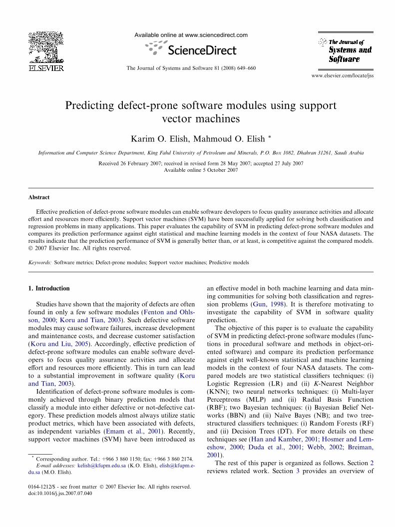
the hyperplane if it is separated without error and the dis-tance (margin) between the closest vectors to the hyper-plane is maximal (Abe, 2005). Fig. 1a shows the linearseparation of two classes by SVM in two-dimensionalspace. Circles represent (class A) and squares represent(class B). The SVM attempts to place a linear boundary(solid line) between the two different classes and draw thisline in such a way that the margin space between dottedlines is maximized.

In a binary category classification problem, we have toestimate a function f : Rp 7!f�1g using training data. Letus represent the class A with x 2 A, y = 1 and class B withx 2 B; y ¼ �1; ðxi; yiÞ 2 Rp � f�1g. If the training data arelinearly separable by hyperplane in the p dimensional spacethen there exists a pair (w,b) such that:

wTxi þ b P þ1 for all xi 2 A

wTxi þ b 6 �1 for all xi 2 Bð1Þ

for all i = 1,2, . . . ,n; where w is a p-dimensional vectororthogonal to the hyperplane and b is the bias term. Theinequality constraints (1) can be combined to give:

yiðwTxi þ bÞP 1 for all xi 2 A [ B ð2Þ

MaximumMargin

Optimalhyperplane

iξ

jξ

MaximumMargin

Optimalhyperplane

Support Vectors

hyperplane

hyperplane

a b

Fig. 1. (a) Optimal separating hyperplane for separable case in 2D space, (b) linear separating hyperplane for non-separable case in 2D space.

K.O. Elish, M.O. Elish / The Journal of Systems and Software 81 (2008) 649–660 651

The maximal margin classifier optimizes this by separatingthe data with the maximal margin hyperplane. The learningproblem is reformulated as: minimize kwk2 = wTw subjectto the constraints of linear separability (2). The optimiza-tion is now a quadratic programming (QP) problem:

Minimizew;b

1

2kwk2

� �ð3Þ

Subject to yiðwTxi þ bÞP 1; i ¼ 1; . . . ; n ð4Þ

where (xi,yi) is the training set, and n is the number oftraining sets. By using standard Lagrangian duality tech-niques, and after further simplification (See Vapnik(1995) or Burges (1998) for derivation details.), the follow-ing is the dual form of the optimization problem:

F ðkÞ ¼Xn

i¼1

ki �1

2kwk2

¼Xn

i¼1

ki �1

2

Xn

i¼1

Xn

j¼1

kikjyiyjxTi xj ð5Þ

where k = (k1, . . . ,kn)T are the Lagrange multipliers and arenon-zero only for the support vectors. The formulated sup-port vector machine is called the hard-margin support vec-tor machine (Abe, 2005). This function has to bemaximized with respect to ki P 0. Therefore, we optimizethe following problem:

MaximizeXn

i¼1

ki �1

2

Xn

i¼1

Xn

j¼1

kikjyiyjxTi xj

( )ð6Þ

Subject toXn

i¼1

kiyi ¼ 0; and ki P 0; i ¼ 1; 2; . . . ; n

ð7Þ

Once the solution has been found in the form of a vectork = (k1, . . . ,kn)T, the optimal separating hyperplane isfound and the decision function is obtained as follows:

f ðxÞ ¼ signXn

i¼1

kiyiðxTi xÞ þ b ð8Þ

3.1.2. The non-separable case

Consider the case where the training data are non-sepa-rable without error. In this case one may want to separatethe training set with a minimal number of errors. Fig. 1bshows the non-separable case of two classes in two-dimen-sional space. Therefore, the minimization problem needs tobe modified to allow misclassified data points. This can bedone by introducing positive slack variables ni P 0 in theconstraints to measure how much the margin constraintsare violated (Cortes and Vapnik, 1995):

Minimizew;b;n

1

2kwk2 þ C

Xn

i¼1

ni

( )ð9Þ

Subject to yiðwTxi þ bÞP 1� ni; for i ¼ 1; . . . ; n ð10Þ

where C is the regularizing (margin) parameter that deter-mines the trade-off between the maximization of the mar-gin and minimization of the classification error (Gun,1998; Cristianini and Shawe-Taylor, 2000). The solutionto this minimization problem is similar to the separablecase except for a modification of the bounds of the La-grange multipliers. Therefore, Eq. (7) is changed to:

Xn

i¼1

kiyi ¼ 0; and 0 6 ki 6 C; i ¼ 1; 2; . . . ; n ð11Þ

Thus the only difference from the separable case is that theki now has an upper bound of C. The obtained support vec-tor machine in this case is called the soft-margin supportvector machine (Abe, 2005).

3.2. Two-class: nonlinear support vector machines

In case that SVM cannot linearly separate two classes,SVM extends its applicability to solve this problem by

3R2R

Data is linearly separable in this new space

Data is not linearly separable

Fig. 2. Mapping input data into higher dimensional space.

1 WEKA (Waikato Environment for Knowledge Analysis). http://www.cs.waikato.ac.nz/~ml/weka/.

2 http://mdp.ivv.nasa.gov/index.html.


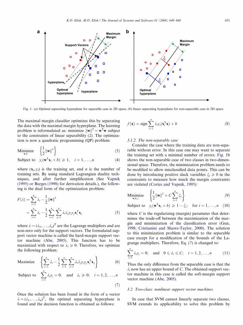
mapping input data into higher dimensional featurespaces using a nonlinear mapping / (Burges, 1998), suchthat x # /(x), where / : Rn ! Rm is the feature map. Itis possible to create a hyperplane that allows linear sepa-ration in high-dimensional space (Burges, 1998). This cor-responds to a curved surface in the lower dimensionalspace. Fig. 2 shows the transformation from lower tohigher dimensional feature spaces using /. This transfor-mation can be done using a kernel function. Therefore,the kernel function is an important parameter in SVM.The kernel function K(xi,xj) is defined as follows (Abe,2005):

Kðxi; xjÞ ¼ /ðxiÞT/ðxjÞ ð12Þ

Therefore, the optimization problem of Eq. (6) becomes:

MaximizeXn

i¼1

ki �1

2

Xn

i¼1

Xn

j¼1

kikjyiyjkðxi; xjÞ( )

ð13Þ

Subject toXn

i¼1

kiyi ¼ 0; and ki P 0; i ¼ 1; 2; . . . ; n

ð14Þ

where K(xi,xj) is the kernel function performing the nonlin-ear mapping into feature space. Once the solution has beenfound, the decision can be constructed as:

f ðxÞ ¼ signXn

i¼1

kiyikðxi; xÞ þ b ð15Þ

The following are the most common kernel functions in lit-erature (Abe, 2005; Gun, 1998; Burges, 1998):

1. Linear: Kðxi; xjÞ ¼ xTi xj.

2. Polynomial: Kðxi; xjÞ ¼ ðxTi xj þ 1Þd .

3. Gaussian (RBF): Kðxi; xjÞ ¼ expð�ckxi � xjk2Þ.4. Sigmoid (MLP): Kðxi; xjÞ ¼ tanhðcðxT

i xjÞ � rÞ.

Gaussian radial basis function (RBF) kernel was used inthis study because it yields better prediction performance(Smola, 1998).

4. Empirical evaluation

This section discusses the conducted empirical studythat evaluates the capability of SVM in predicting defect-

prone software modules. We used the open source WEKA1

machine learning toolkit to conduct this study.

4.1. Goal

Using GQM template (Basili and Rombach, 1988) forgoal definition, the goal of this empirical study is definedas follows: Evaluate SVM for the purpose of predictingdefect-prone software modules with respect to its predictionperformance against the eight compared models (LR,KNN, MLP, RBF, BBN, NB, RF, and DT) from the point

of view of researchers and practitioners in the context of

four NASA datasets.

4.2. Datasets

The datasets used in this study are four mission criticalNASA software projects, which are publicly accessiblefrom the repository of the NASA IV&V Facility MetricsData Program.2 Two datasets (CM1 and PC1) are fromsoftware projects written in a procedural language (C)where a module in this case is a function. The other twodatasets (KC1 and KC3) are from projects written inobject-oriented languages (C++ and Java) where a modulein this case is a method. Each dataset contains 21 softwaremetrics (independent variables) at the module-level and theassociated dependent Boolean variable: Defective (whetheror not the module has any defects). Table 1 summarizessome main characteristics of these datasets.

4.3. Independent variables

The independent variables are 21 static metrics at themodule-level including McCabe (McCabe, 1976; McCabeand Butler, 1989), Halstead (basic and derived) (Halstead,1977), Line Count, and Branch Count. Table 2 lists thesemetrics.

Since some independent variables might be highly corre-lated, a correlation-based feature selection technique (CFS)(Hall, 2000) was applied to down-select the best predictorsout of the 21 independent variables in the datasets. Thisinvolves searching through all possible combinations ofvariables in the dataset to find which subset of variablesworks best for prediction. CFS evaluates each subset ofvariables by considering the individual predictive abilityof each variable along with the degree of redundancybetween them. Table 3 provides the resulted best subsetof independent variables in each dataset.

4.4. Dependent variable

This study focuses on predicting whether a module isdefective or not, rather than how many defects it contains.

http://www.cs.waikato.ac.nz/~ml/weka/

http://www.cs.waikato.ac.nz/~ml/weka/

http://mdp.ivv.nasa.gov/index.html

Table 1Characteristics of datasets

Project Language # of Modules % of Defective modules Description

Procedural CM1 C 496 9.7 NASA spacecraft instrumentPC1 C 1107 6.9 Flight software for an earth orbiting satellite

Object oriented KC1 C++ 2107 15.4 Storage management for receiving and processing ground dataKC3 Java 458 6.3 Collection, processing and delivery of satellite metadata

Table 2Module-level metrics (independent variables)

Metric Type Definition

V (g) McCabe Cyclomatic ComplexityEV (g) McCabe Essential ComplexityIV (g) McCabe Design ComplexityLOC McCabe Total lines of code

N DerivedHalstead

Total number of operands andoperators

V DerivedHalstead

Volume on minimalimplementation

L DerivedHalstead

Program Length = V/N

D DerivedHalstead

Difficulty = 1/L

I DerivedHalstead

Intelligent count

E DerivedHalstead

Effort to write program = V/L

B DerivedHalstead

Effort Estimate

T DerivedHalstead

Time to write program = E/18 s

LOCode Line Count Number of lines of statementLOComment Line Count Number of lines of commentLOBlank Line Count Number of lines of blankLOCodeAndComment Line Count Number of lines of code and

comment

UniqOp BasicHalstead

Number of Unique operators

UniqOpnd BasicHalstead

Number of Unique operands

TotalOp BasicHalstead

Total number of operators

TotalOpnd BasicHalstead

Total number of operands

BranchCount Branch Total number of branch count

Table 3Best subset of independent variables in each dataset

Dataset Best subset of independent variables

CM1 LOC, IV(g), D, I, LOComment, LOBlank,PC1 V(g), I, LOCodeAndComment, LOComment, LOBlank,

UniqOpKC1 V, D, V(g), LOCode, LOComment, LOBlank, UniqOpndKC3 N, EV(g), LOCodeAndComment

Table 4A confusion matrix

Predicted

Not defective Defective

Actual Not defective TN = True Negative FP = False PositiveDefective FN = False Negative TP = True Positive


Accordingly, the dependent variable is a Boolean variable:Defective (whether or not the module has any defects). Pre-dicting the number of defects is a possible future work ifsuch data is available.

4.5. Prediction performance measures

The performance of prediction models for two-classproblem (e.g. defective or not defective) is typically evalu-ated using a confusion matrix, which is shown in Table 4.In this study, we used the commonly used prediction per-formance measures (Witten and Frank, 2005): accuracy,precision, recall and F-measure to evaluate and compareprediction models quantitatively. These measures arederived from the confusion matrix.

4.5.1. Accuracy

Accuracy is also known as correct classification rate. Itis defined as the ratio of the number of modules correctlypredicted to the total number of modules. It is calculatedas follows:

Accuracy ¼ TP þ TNTP þ TN þ FP þ FN

4.5.2. Precision

Precision is also known as correctness. It is defined asthe ratio of the number of modules correctly predicted asdefective to the total number of modules predicted asdefective. It is calculated as follows:

Precision ¼ TPTP þ FP

4.5.3. Recall

Recall is also known as defect detection rate. It isdefined as the ratio of the number of modules correctly pre-dicted as defective to the total number of modules that areactually defective. It is calculated as follows:

Recall ¼ TPTP þ FN

Both precision and recall are important performancemeasures. The higher the precision, the less effort wastedin testing and inspection; and the higher the recall, thefewer defective modules go undetected (Koru and Liu,


2005). However, there is a trade-off between precision andrecall (Witten and Frank, 2005; Koru and Liu, 2005). Forexample, if a model predicts only one module as defectiveand this module is actually defective, the model’s preci-sion will be one. However, the model’s recall will below if there are other defective modules. As anotherexample, if a model predicts all modules as defective,its recall will be one but its precision will be low. There-fore, F-measure is needed which combines recall and pre-cision in a single efficiency measure (Witten and Frank,2005).

4.5.4. F-measure

F-measure considers both precision and recall equallyimportant by taking their harmonic mean (Witten andFrank, 2005). It is calculated as follows:

F -measure ¼ 2 � Precision � RecallPrecisionþ Recall

4.6. Parameters initialization

The parameters for each of the investigated predictionmodel were initialized mostly with the default settings ofthe WEKA toolkit as follows:

• Support vector machines (SVM): the regularizationparameter (C) was set at 1; the kernel function usedwas Gaussian (RBF); and the bandwidth (c) of the ker-nel function was set at 0.5.

• Logistic regression (LR): the method of optimizationwas the maximization of log-likelihood.

• K-nearest neighbor (KNN): the number of observations(k) in the set of closest neighbor was set at 3.

• Multi-layer perceptrons (MLP): a three layered, fullyconnected, feedforward multi-Layer perceptron (MLP)was used as network architecture. MLP was trainedusing backpropagation algorithm. The number of hid-den nodes varied based on the size and nature of thedatasets. Therefore, we used MLP with 4 hidden nodesfor CM1 and PC1 datasets; 5 hidden nodes for KC1dataset; and 3 hidden nodes for KC3 dataset. All nodesin the network used the sigmoid transfer function. Thelearning rate was initially 0.3 and the momentum termwas set at 0.2. The algorithm was halted when therehad been no significant reduction in training error for500 epochs with a tolerance value to convergence of0.01.

• Radial basis function (RBF): k-means clustering algo-rithm was used to determine the RBF center c and widthr. The value of k was set at 2.

• Bayesian belief network (BBN): the SimpleEstimatoralgorithm was used for finding the conditional probabil-ity tables and the hill climbing algorithm was used forsearching the network.

• Naı̈ve Bayes (NB): it does not require any parameters topass.

• Random forest (RF): the number of trees to be generatedwas set at 10; the number of input variables randomlyselected at each node was set at 2; and each tree grownto the largest extent possible, i.e. the maximum depth ofthe trees is unlimited.

• Decision tree (DT): it uses the well-known C4.5 algo-rithm to generate decision tree. The confidence factorused for pruning was set at 25% and the minimum num-ber of instances per leaf was set at 2.

In addition to the above parameters initialization, adefault threshold (cut-off) of 0.5 was used for all modelsto classify a module as defect-prone if its predicted proba-bility is higher than the threshold.

4.7. Cross-validation

A 10-fold cross-validation (Kohavi, 1995) was used toevaluate the performance of the prediction models. Eachdataset was randomly partitioned into 10 bins of equal size.For 10 times, 9 bins were picked to train the models andthe remaining bin was used to test them, each time leavingout a different bin. This cross-validation process was run100 times, using different randomization seed values forcross-validation shuffling in each run to ensure low bias.We then computed the mean and the standard deviationfor each performance measure over these 100 differentruns. The achieved results by each prediction model arereported in Tables 5–8 for the CM1, PC1, KC1 and KC3datasets respectively.

4.8. Significance test

We performed the corrected resampled t-test (Nadeauand Bengio, 2003) at 0.05 level of significance (95% confi-dence level) to determine whether or not there is a signifi-cant difference between the prediction performance ofSVM and the other compared models. The correctedresampled t-test is more appropriate than the standard t-test in the case of using x-fold cross-validation becausethe standard t-test may generate too many significant dif-ferences due to dependencies in the estimates (Dietterich,1998). The results of the corrected resampled t-test arereported in the ‘Sig?’ columns of Tables 5–8. In these col-umns, Yes means that there is a significant performancedifference between SVM and the corresponding model,and No means that there is no significant difference. Inaddition, a (+) means that SVM outperforms the corre-sponding model, and a (�) means that SVM isoutperformed.

4.9. Discussion of results

Figs. 3 and 4 plot the mean versus the standard devia-tion of the accuracy and the F-measure that are achievedby each model using CM1 dataset respectively. A good pre-diction model should appear in the upper left corner of

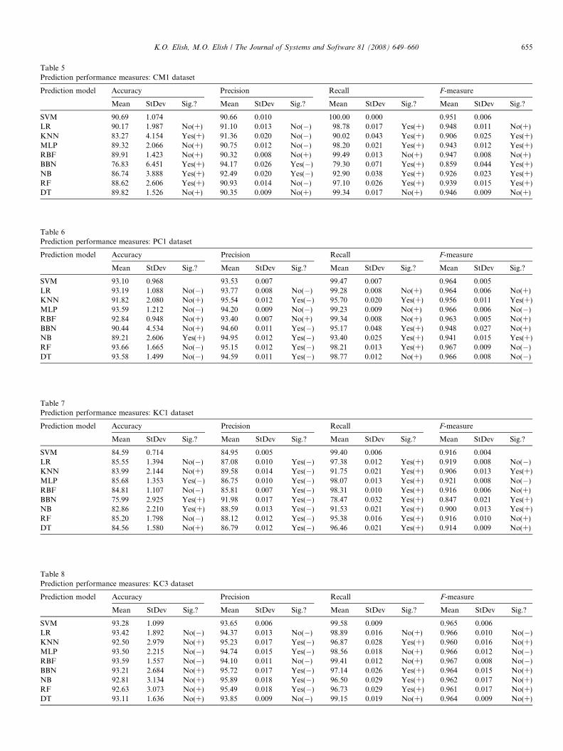
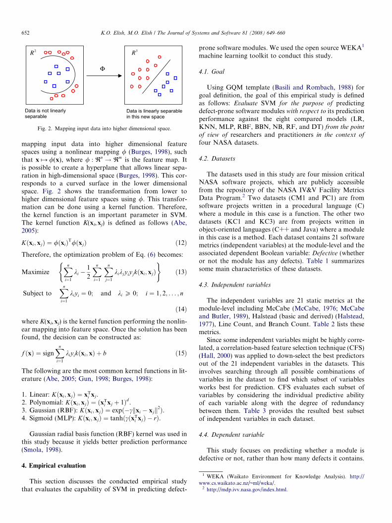
Table 5Prediction performance measures: CM1 dataset

Prediction model Accuracy Precision Recall F-measure

Mean StDev Sig.? Mean StDev Sig.? Mean StDev Sig.? Mean StDev Sig.?

SVM 90.69 1.074 90.66 0.010 100.00 0.000 0.951 0.006LR 90.17 1.987 No(+) 91.10 0.013 No(�) 98.78 0.017 Yes(+) 0.948 0.011 No(+)KNN 83.27 4.154 Yes(+) 91.36 0.020 No(�) 90.02 0.043 Yes(+) 0.906 0.025 Yes(+)MLP 89.32 2.066 No(+) 90.75 0.012 No(�) 98.20 0.021 Yes(+) 0.943 0.012 Yes(+)RBF 89.91 1.423 No(+) 90.32 0.008 No(+) 99.49 0.013 No(+) 0.947 0.008 No(+)BBN 76.83 6.451 Yes(+) 94.17 0.026 Yes(�) 79.30 0.071 Yes(+) 0.859 0.044 Yes(+)NB 86.74 3.888 Yes(+) 92.49 0.020 Yes(�) 92.90 0.038 Yes(+) 0.926 0.023 Yes(+)RF 88.62 2.606 Yes(+) 90.93 0.014 No(�) 97.10 0.026 Yes(+) 0.939 0.015 Yes(+)DT 89.82 1.526 No(+) 90.35 0.009 No(+) 99.34 0.017 No(+) 0.946 0.009 No(+)

Table 6Prediction performance measures: PC1 dataset



SVM 93.10 0.968 93.53 0.007 99.47 0.007 0.964 0.005LR 93.19 1.088 No(�) 93.77 0.008 No(�) 99.28 0.008 No(+) 0.964 0.006 No(+)KNN 91.82 2.080 No(+) 95.54 0.012 Yes(�) 95.70 0.020 Yes(+) 0.956 0.011 Yes(+)MLP 93.59 1.212 No(�) 94.20 0.009 No(�) 99.23 0.009 No(+) 0.966 0.006 No(�)RBF 92.84 0.948 No(+) 93.40 0.007 No(+) 99.34 0.008 No(+) 0.963 0.005 No(+)BBN 90.44 4.534 No(+) 94.60 0.011 Yes(�) 95.17 0.048 Yes(+) 0.948 0.027 No(+)NB 89.21 2.606 Yes(+) 94.95 0.012 Yes(�) 93.40 0.025 Yes(+) 0.941 0.015 Yes(+)RF 93.66 1.665 No(�) 95.15 0.012 Yes(�) 98.21 0.013 Yes(+) 0.967 0.009 No(�)DT 93.58 1.499 No(�) 94.59 0.011 Yes(�) 98.77 0.012 No(+) 0.966 0.008 No(�)

Table 7Prediction performance measures: KC1 dataset



SVM 84.59 0.714 84.95 0.005 99.40 0.006 0.916 0.004LR 85.55 1.394 No(�) 87.08 0.010 Yes(�) 97.38 0.012 Yes(+) 0.919 0.008 No(�)KNN 83.99 2.144 No(+) 89.58 0.014 Yes(�) 91.75 0.021 Yes(+) 0.906 0.013 Yes(+)MLP 85.68 1.353 Yes(�) 86.75 0.010 Yes(�) 98.07 0.013 Yes(+) 0.921 0.008 No(�)RBF 84.81 1.107 No(�) 85.81 0.007 Yes(�) 98.31 0.010 Yes(+) 0.916 0.006 No(+)BBN 75.99 2.925 Yes(+) 91.98 0.017 Yes(�) 78.47 0.032 Yes(+) 0.847 0.021 Yes(+)NB 82.86 2.210 Yes(+) 88.59 0.013 Yes(�) 91.53 0.021 Yes(+) 0.900 0.013 Yes(+)RF 85.20 1.798 No(�) 88.12 0.012 Yes(�) 95.38 0.016 Yes(+) 0.916 0.010 No(+)DT 84.56 1.580 No(+) 86.79 0.012 Yes(�) 96.46 0.021 Yes(+) 0.914 0.009 No(+)

Table 8Prediction performance measures: KC3 dataset



SVM 93.28 1.099 93.65 0.006 99.58 0.009 0.965 0.006LR 93.42 1.892 No(�) 94.37 0.013 No(�) 98.89 0.016 No(+) 0.966 0.010 No(�)KNN 92.50 2.979 No(+) 95.23 0.017 Yes(�) 96.87 0.028 Yes(+) 0.960 0.016 No(+)MLP 93.50 2.215 No(�) 94.74 0.015 Yes(�) 98.56 0.018 No(+) 0.966 0.012 No(�)RBF 93.59 1.557 No(�) 94.10 0.011 No(�) 99.41 0.012 No(+) 0.967 0.008 No(�)BBN 93.21 2.684 No(+) 95.72 0.017 Yes(�) 97.14 0.026 Yes(+) 0.964 0.015 No(+)NB 92.81 3.134 No(+) 95.89 0.018 Yes(�) 96.50 0.029 Yes(+) 0.962 0.017 No(+)RF 92.63 3.073 No(+) 95.49 0.018 Yes(�) 96.73 0.029 Yes(+) 0.961 0.017 No(+)DT 93.11 1.636 No(+) 93.85 0.009 No(�) 99.15 0.019 No(+) 0.964 0.009 No(+)


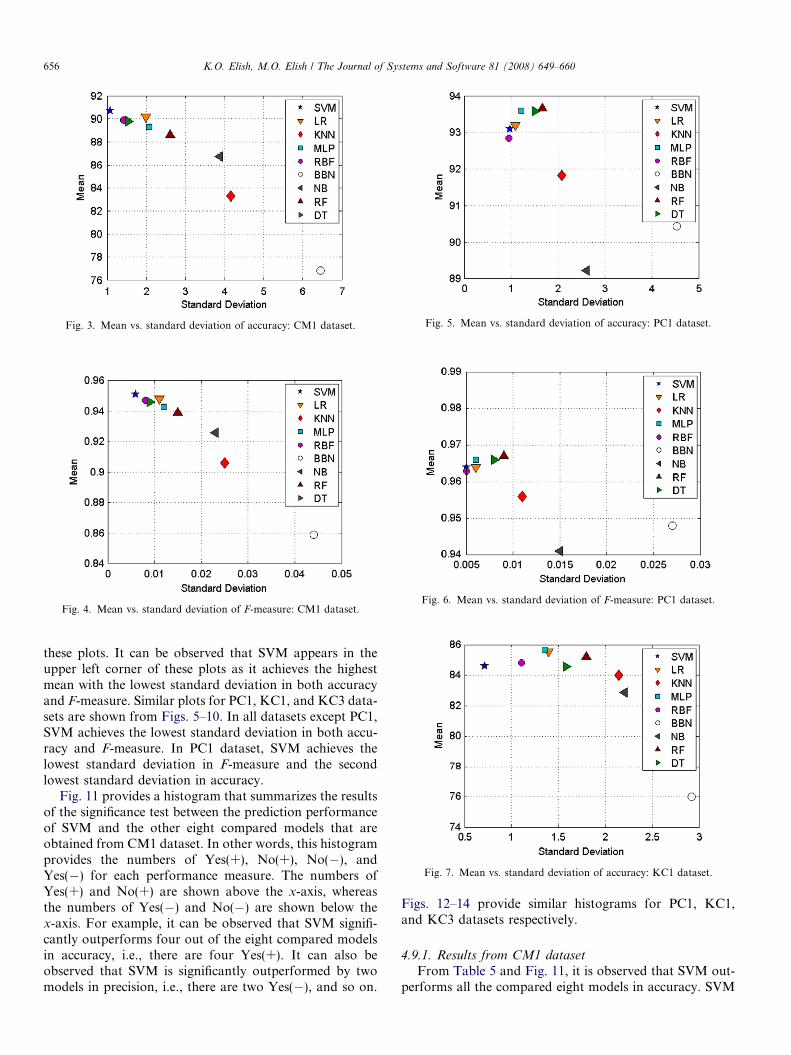
Fig. 3. Mean vs. standard deviation of accuracy: CM1 dataset.

Fig. 4. Mean vs. standard deviation of F-measure: CM1 dataset.

Fig. 5. Mean vs. standard deviation of accuracy: PC1 dataset.

Fig. 6. Mean vs. standard deviation of F-measure: PC1 dataset.

Fig. 7. Mean vs. standard deviation of accuracy: KC1 dataset.


these plots. It can be observed that SVM appears in theupper left corner of these plots as it achieves the highestmean with the lowest standard deviation in both accuracyand F-measure. Similar plots for PC1, KC1, and KC3 data-sets are shown from Figs. 5–10. In all datasets except PC1,SVM achieves the lowest standard deviation in both accu-racy and F-measure. In PC1 dataset, SVM achieves thelowest standard deviation in F-measure and the secondlowest standard deviation in accuracy.

Fig. 11 provides a histogram that summarizes the resultsof the significance test between the prediction performanceof SVM and the other eight compared models that areobtained from CM1 dataset. In other words, this histogramprovides the numbers of Yes(+), No(+), No(�), andYes(�) for each performance measure. The numbers ofYes(+) and No(+) are shown above the x-axis, whereasthe numbers of Yes(�) and No(�) are shown below thex-axis. For example, it can be observed that SVM signifi-cantly outperforms four out of the eight compared modelsin accuracy, i.e., there are four Yes(+). It can also beobserved that SVM is significantly outperformed by twomodels in precision, i.e., there are two Yes(�), and so on.

Figs. 12–14 provide similar histograms for PC1, KC1,and KC3 datasets respectively.

4.9.1. Results from CM1 datasetFrom Table 5 and Fig. 11, it is observed that SVM out-

performs all the compared eight models in accuracy. SVM

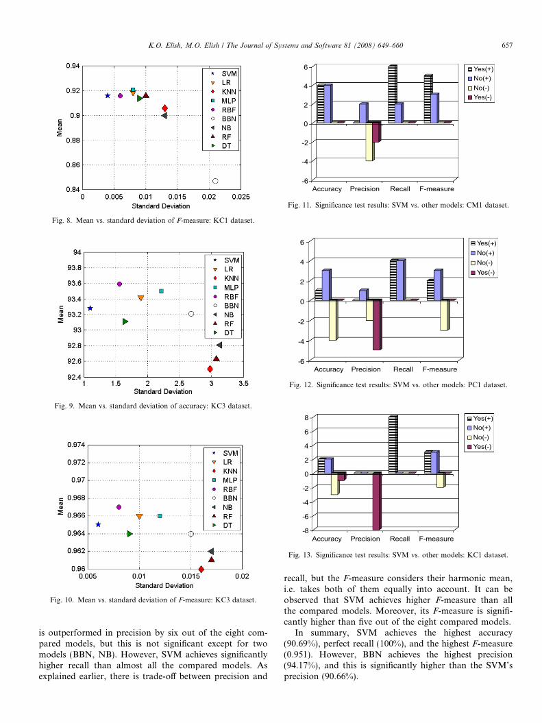
Fig. 8. Mean vs. standard deviation of F-measure: KC1 dataset.

Fig. 9. Mean vs. standard deviation of accuracy: KC3 dataset.

Fig. 10. Mean vs. standard deviation of F-measure: KC3 dataset.

-6

-4

-2

0

2

4

6

Accuracy Precision Recall

Yes(+)No(+)No(-)Yes(-)

F-measure

Fig. 11. Significance test results: SVM vs. other models: CM1 dataset.

-6

-4

-2

0

2

4

6


Yes(+)

No(+)

No(-)

Yes(-)

F-measure

Fig. 12. Significance test results: SVM vs. other models: PC1 dataset.

-8

-6

-4

-2

0

2

4

6

8



F-measure

Fig. 13. Significance test results: SVM vs. other models: KC1 dataset.


is outperformed in precision by six out of the eight com-pared models, but this is not significant except for twomodels (BBN, NB). However, SVM achieves significantlyhigher recall than almost all the compared models. Asexplained earlier, there is trade-off between precision and

recall, but the F-measure considers their harmonic mean,i.e. takes both of them equally into account. It can beobserved that SVM achieves higher F-measure than allthe compared models. Moreover, its F-measure is signifi-cantly higher than five out of the eight compared models.

In summary, SVM achieves the highest accuracy(90.69%), perfect recall (100%), and the highest F-measure(0.951). However, BBN achieves the highest precision(94.17%), and this is significantly higher than the SVM’sprecision (90.66%).

-6

-4

-2

0

2

4

6



F-measure

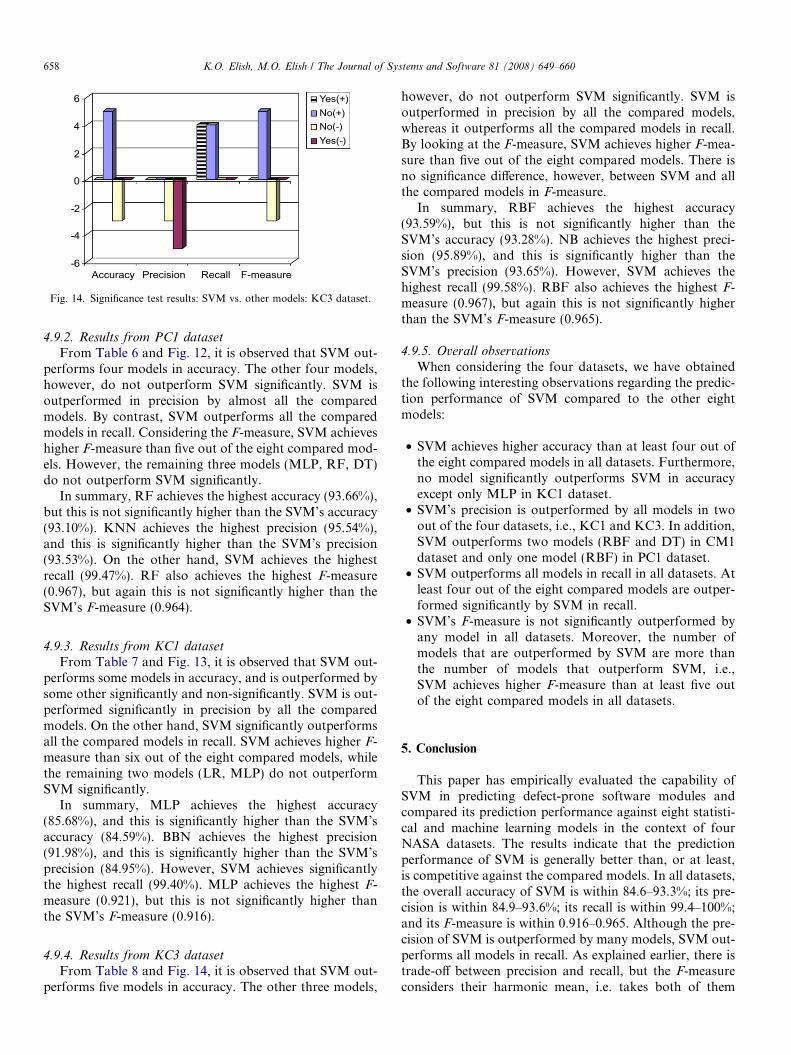
Fig. 14. Significance test results: SVM vs. other models: KC3 dataset.


4.9.2. Results from PC1 datasetFrom Table 6 and Fig. 12, it is observed that SVM out-

performs four models in accuracy. The other four models,however, do not outperform SVM significantly. SVM isoutperformed in precision by almost all the comparedmodels. By contrast, SVM outperforms all the comparedmodels in recall. Considering the F-measure, SVM achieveshigher F-measure than five out of the eight compared mod-els. However, the remaining three models (MLP, RF, DT)do not outperform SVM significantly.

In summary, RF achieves the highest accuracy (93.66%),but this is not significantly higher than the SVM’s accuracy(93.10%). KNN achieves the highest precision (95.54%),and this is significantly higher than the SVM’s precision(93.53%). On the other hand, SVM achieves the highestrecall (99.47%). RF also achieves the highest F-measure(0.967), but again this is not significantly higher than theSVM’s F-measure (0.964).

4.9.3. Results from KC1 datasetFrom Table 7 and Fig. 13, it is observed that SVM out-

performs some models in accuracy, and is outperformed bysome other significantly and non-significantly. SVM is out-performed significantly in precision by all the comparedmodels. On the other hand, SVM significantly outperformsall the compared models in recall. SVM achieves higher F-measure than six out of the eight compared models, whilethe remaining two models (LR, MLP) do not outperformSVM significantly.

In summary, MLP achieves the highest accuracy(85.68%), and this is significantly higher than the SVM’saccuracy (84.59%). BBN achieves the highest precision(91.98%), and this is significantly higher than the SVM’sprecision (84.95%). However, SVM achieves significantlythe highest recall (99.40%). MLP achieves the highest F-measure (0.921), but this is not significantly higher thanthe SVM’s F-measure (0.916).

4.9.4. Results from KC3 datasetFrom Table 8 and Fig. 14, it is observed that SVM out-

performs five models in accuracy. The other three models,

however, do not outperform SVM significantly. SVM isoutperformed in precision by all the compared models,whereas it outperforms all the compared models in recall.By looking at the F-measure, SVM achieves higher F-mea-sure than five out of the eight compared models. There isno significance difference, however, between SVM and allthe compared models in F-measure.

In summary, RBF achieves the highest accuracy(93.59%), but this is not significantly higher than theSVM’s accuracy (93.28%). NB achieves the highest preci-sion (95.89%), and this is significantly higher than theSVM’s precision (93.65%). However, SVM achieves thehighest recall (99.58%). RBF also achieves the highest F-measure (0.967), but again this is not significantly higherthan the SVM’s F-measure (0.965).

4.9.5. Overall observations

When considering the four datasets, we have obtainedthe following interesting observations regarding the predic-tion performance of SVM compared to the other eightmodels:

• SVM achieves higher accuracy than at least four out ofthe eight compared models in all datasets. Furthermore,no model significantly outperforms SVM in accuracyexcept only MLP in KC1 dataset.

• SVM’s precision is outperformed by all models in twoout of the four datasets, i.e., KC1 and KC3. In addition,SVM outperforms two models (RBF and DT) in CM1dataset and only one model (RBF) in PC1 dataset.

• SVM outperforms all models in recall in all datasets. Atleast four out of the eight compared models are outper-formed significantly by SVM in recall.

• SVM’s F-measure is not significantly outperformed byany model in all datasets. Moreover, the number ofmodels that are outperformed by SVM are more thanthe number of models that outperform SVM, i.e.,SVM achieves higher F-measure than at least five outof the eight compared models in all datasets.

5. Conclusion

This paper has empirically evaluated the capability ofSVM in predicting defect-prone software modules andcompared its prediction performance against eight statisti-cal and machine learning models in the context of fourNASA datasets. The results indicate that the predictionperformance of SVM is generally better than, or at least,is competitive against the compared models. In all datasets,the overall accuracy of SVM is within 84.6–93.3%; its pre-cision is within 84.9–93.6%; its recall is within 99.4–100%;and its F-measure is within 0.916–0.965. Although the pre-cision of SVM is outperformed by many models, SVM out-performs all models in recall. As explained earlier, there istrade-off between precision and recall, but the F-measureconsiders their harmonic mean, i.e. takes both of them


equally into account. When considering the F-measure,SVM achieves higher F-measure than at least five out ofthe eight compared models in all datasets, and is not signif-icantly outperformed by any model.

The results reveal the effectiveness of SVM in predictingdefect-prone software modules, and thus suggest that it canbe useful and practical addition to the framework of soft-ware quality prediction. Moreover, the superior perfor-mance of SVM, especially in recall, can have a practicalimplication in the context of software testing by reducingthe risks of defective modules go undetected.

One direction of future work would be conductingadditional empirical studies with other datasets to furthersupport the findings of this paper, and to realize the fullpotential and possible limitation of SVM. Another possi-ble direction of future work would be considering addi-tional independent variables such as coupling andcohesion metrics if information on such metrics is avail-able. Finally, it would be interesting to apply SVM in pre-dicting other software quality attributes in addition todefects.

Acknowledgements

The authors would like to thank the anonymous review-ers for their constructive comments. The authors alsoacknowledge the support of King Fahd University ofPetroleum and Minerals in the development of this work.

References

Abe, S., 2005. Support Vector Machines for Pattern Classification.Springer, USA.

Azar, D., Bouktif, S., K’egl, B., Sahraoui, H., Precup, D., 2002.Combining and adapting software quality predictive models bygenetic algorithms. In: Proceedings of the 17th IEEE InternationalConference on Automated Software Engineering (ASE2002), pp. 285–288.

Bao, L., Sun, Z., 2002. Identifying genes related to drug anticancermechanisms using support vector machine. FEBS Letters 521, 109–114.

Basili, V., Rombach, H., 1988. The TAME project: towards improvement-oriented software environment. IEEE Transactions on SoftwareEngineering 14 (6), 758–773.

Basili, V., Briand, L., Melo, W., 1996. A validation of object-orienteddesign metrics as quality indicators. IEEE Transactions on SoftwareEngineering 22 (10), 751–761.

Breiman, L., 2001. Random forests. Machine Learning 45, 5–32.Briand, L.C., Basili, V., Hetmanski, C., 1993. Developing interpretable

models with optimized set reduction for identifying high-risk softwarecomponents. IEEE Transactions on Software Engineering 19 (11),1028–1044.

Burbidge, R., Trotter, M., Buxton, B., Holden, S., 2001. Drug design bymachine learning: support vector machines for pharmaceutical dataanalysis. Computers and Chemistry 26, 5–14.

Burges, C., 1998. A tutorial on support vector machines for patternrecognition. Data Mining and Knowledge Discovery 2, 121–167.

Cai, Y.-D., Lin, X.-J., Xu, X.-B., Chou, K.-C., 2002. Prediction of proteinstructural classes by support vector machines. Computers and Chem-istry 26, 293–296.

Chen, W., Hsu, S., Shen, H., 2005. Application of SVM and ANN forintrusion detection. Computers and Operations Research 32, 2617–2634.

Chidamber, S., Kemerer, C., 1994. A metrics suite for object-orienteddesign. IEEE Transactions on Software Engineering 20 (6), 476–493.

Cortes, C., Vapnik, V., 1995. Support-vector networks. Machine Learning20, 273–297.

Cristianini, N., Shawe-Taylor, J., 2000. An Introduction to SupportVector Machines and Other Kernel-based Learning Methods. Cam-bridge University Press, Cambridge, UK.

Dietterich, T., 1998. Approximate statistical tests for comparing supervisedclassification learning algorithms. Neural Computation 10, 1895–1924.

Drucker, H., Wu, D., Vapnik, V., 1999. Support vector machines for spamcategorization. IEEE Transactions on Neural Networks 10 (5), 1048–1054.

Duda, R., Hart, P., Stork, D., 2001. Pattern Classification, second ed.John Wiley & Sons, New York.

Dumais, S., 1998. Using SVMS for text categorization. IEEE IntelligentSystems 13 (4), 21–23.

Emam, K., Benlarbi, S., Goel, N., Rai, S., 2001. Comparing case-basedreasoning classifiers for predicting high risk software components.Journal of Systems and Software 55 (3), 301–310.

Fenton, N., Ohlsson, N., 2000. Quantitative analysis of faults and failuresin a complex software system. IEEE Transactions on SoftwareEngineering 26 (8), 797–814.

Fenton, N., Neil, M., Krause, P., 2002. Software measurement: uncer-tainty and causal modeling. IEEE Software 19, 116–122.

Gun, S., 1998. Support vector machines for classification and regression.Technical Report, University of Southampton.

Guo, L., Cukic, B., Singh, H., 2003. Predicting fault prone modules by theDempster–Shafer belief networks. In: Proceedings of the 18th IEEEInternational Conference on Automated Software Engineering (ASE2003), pp. 249–252.

Guo, L., Ma, Y., Cukic, B., Singh, H., 2004. Robust prediction of fault-proneness by random forests. In: Proceedings of the 15th InternationalSymposium on Software Reliability Engineering (ISSRE’04), pp. 417–428.

Hall, M., 2000. Correlation-based feature selection for discrete andnumeric class machine learning. In: Proceedings of the 17th Interna-tional Conference on Machine Learning, pp. 359–366.

Halstead, M., 1977. Elements of Software Science. Elsevier.Han, J., Kamber, M., 2001. Data Mining: Concepts and Techniques,

second ed. Morgan Kauffman.Hosmer, D., Lemeshow, S., 2000. Applied Logistic Regression, second ed.

John Wiley & Sons, New York.Khoshgoftaar, T., Allen, E., Kalaichelvan, K., Goel, N., 1996. Early

quality prediction: a case study in telecommunications. IEEE Software13 (1), 65–71.

Khoshgoftaar, T., Allen, E., Hudepohl, J., Aud, S., 1997. Application ofneural networks to software quality modeling of a very largetelecommunications system. IEEE Transactions on Neural Networks8 (4), 902–909.

Khoshgoftaar, T., Allen, E., Deng, J., 2002. Using regression trees toclassify fault-prone software modules. IEEE Transactions on Reliabil-ity 51 (4), 455–462.

Kohavi, R., 1995. A study of cross-validation and bootstrap for accuracyestimation and model selection. In: Proceedings of the 14th Interna-tional Joint Conference on Artificial Intelligence (IJCAI), pp. 1137–1143.

Koru, A., Liu, H., 2005. Building effective defect-prediction models inpractice. IEEE Software, 23–29.

Koru, A., Tian, J., 2003. An empirical comparison and characterization ofhigh defect and high complexity modules. Journal of Systems andSoftware 67, 153–163.

Lin, S., Patel, S., Duncan, A., Goodwin, L., 2003. Using decision trees andsupport vector machines to classify genes by names. In: Proceedings ofthe European Workshop on Data Mining and Text Mining forBioinformatics, pp. 35–41.

Ma, Y., Guo, L., Cukic, B., 2006. A Statistical Framework for thePrediction of Fault-Proneness. Advances in Machine Learning Appli-cation in Software Engineering. Idea Group Inc..


Mair, C., Kadoda, G., Leflel, M., Phapl, L., Schofield, K., Shepperd, M.,Webster, S., 2000. An investigation of machine learning basedprediction systems. Journal of Systems and Software 53 (1), 23–29.

McCabe, T., 1976. A complexity measure. IEEE Transactions on SoftwareEngineering 2 (4), 308–320.

McCabe, T., Butler, C., 1989. Design complexity measurement andtesting. Communications of the ACM 32 (12), 1415–1425.

Morris, C., Autret, A., Boddy, L., 2001. Support vector machines foridentifying organisms-a comparison with strongly partitioned radialbasis function networks. Ecological Modeling 146, 57–67.

Munson, J., Khoshgoftaar, T., 1992. The detection of fault-proneprograms. IEEE Transactions on Software Engineering 18 (5), 423–433.

Nadeau, C., Bengio, Y., 2003. Inference for the generalization error.Machine Learning 52, 239–281.

Osuna, E., Freund, R., Girosi, F., 1997. Training support vector machines:an application to face detection. In: Proceedings of the IEEE Conferenceon Computer Vision and Pattern Recognition, pp. 130–136.

Schmidt, M., Gish, H., 1996. Speaker identification via support vectorclassifiers. In: Proceedings of the IEEE International Conference onAcoustics, Speech, and Signal Processing (ICASSP-96), pp. 105–108.

Schneidewind, N., 1992. Methodology for validating software metrics.IEEE Transactions on Software Engineering 18 (5), 410–422.

Selby, R., Porter, A., 1988. Learning from examples: generation andevaluation of decision trees for software resource analysis. IEEETransactions on Software Engineering 14 (12), 1743–1756.

Shepperd, M., Kadoda, G., 2001. Comparing software prediction tech-niques using simulation. IEEE Transactions on Software Engineering27 (11), 1014–1022.

Smola, A., 1998. Learning with kernels. Ph.D. dissertation, Department ofComputer Science, Technical University Berlin, Germany.

Tay, F., Cao, L., 2001. Application of support vector machines in financialtime series forecasting. Omega 29, 309–317.

Vapnik, V., 1995. The Nature of Statistical Learning Theory. Springer,New York.

Weaver, R., 2003. The safety of software – Constructing and assuringarguments. Ph.D. dissertation, Department of Computer Science,University of York.

Webb, R., 2002. Statistical Pattern Recognition, second ed. John Wiley &Sons, New York.

Witten, I., Frank, E., 2005. Data Mining: Practical Machine LearningTools and Techniques, second ed. Morgan Kaufmann, San Francisco.

Karim O. Elish is a MS candidate and research assistant in the Informa-tion and Computer Science Department at King Fahd University ofPetroleum and Minerals (KFUPM), Saudi Arabia. He received the BSdegree in computer science from KFUPM in 2006. He is a member ofSoftware Engineering Research Group (SERG) at KFUPM. His mainresearch interests include software metrics and measurement, empiricalsoftware engineering, and application of machine learning and datamining in software engineering.

Mahmoud O. Elish received the PhD degree in computer science fromGeorge Mason University, USA, in 2005. He is an assistant professor inthe Information and Computer Science Department at King Fahd Uni-versity of Petroleum and Minerals, Saudi Arabia. His research interestsinclude software metrics and measurement, object-oriented analysis anddesign, empirical software engineering, and software quality predictivemodels.

predicting defect-prone software modules using support vector machines

Documents