predicting customer repeat purchase and product return
TRANSCRIPT
(Cokal, 2005)
Business Administration 2015-2016
Draft version of the master thesis in Marketing
University of Amsterdam
Faculty of Economics and Businesses
Author: dr. M. M. van der Kuyp (10266313)
[email protected]/ [email protected]
Supervisor: dr. E. Kormaz
Second Reader: dr. U. Konus
Submission date: 24 June 2016
Predicting Customer Repeat Purchase and
Product Return Behavior for Brick-and-Mortar
Grocery Retailers An Empirical Study using Probabilistic Customer-base Analysis Models
Table of Contents
Abstract ........................................................................................................................................... 1
I. Introduction ................................................................................................................................. 2
II. Literature review ....................................................................................................................... 7
Academic and managerial contributions ...................................................................................... 9
III. Theoretical background ........................................................................................................ 11
Theories on past purchase behavior and product return behavior .............................................. 11
IV. Research design ...................................................................................................................... 16
Data ............................................................................................................................................. 16
Key variables .............................................................................................................................. 20
Method ........................................................................................................................................ 22
V. Results ....................................................................................................................................... 23
Preliminary analysis ................................................................................................................... 23
Explanatory analysis ................................................................................................................... 28
VI. Discussion ............................................................................................................................... 37
VII. Conclusion ............................................................................................................................. 41
VIII. Bibliography ........................................................................................................................ 44
IX. Appendix ................................................................................................................................. 48
Figures ........................................................................................................................................ 48
Tables.......................................................................................................................................... 49
Syntax ......................................................................................................................................... 51
Data cleaning .......................................................................................................................... 51
Variable computation .............................................................................................................. 52
Statistical analyses .................................................................................................................. 55

Master thesis, van der Kuyp (2016) Page 1 of 57
Abstract
In recent years, various academic studies focused on predicting repeat purchase behavior
using probabilistic modeling approaches. Main purpose of this study is to contribute to this
literature by investigating the relationship between the past purchase behavior including the
product return behavior and the future repeat purchase behavior in a brick and mortar grocery
retail setting. Based on the expectancy-disconfirmation model, it is expected that consumers who
returned more products will have less number of future repeat purchases. In other words,
customers who return more products are more likely to be disgusted and therefore drop-out.
The study uses transaction data on 4.014 customers of a brick-and-mortar grocery retailer
with the timespan of March 2, 2012 through March 30 2013. The data is gathered from Kaggle,
which is an open source platform that organizes competition among data scientists. The BG/NBD
model of Fader et al (2005) has been used to predict repeat purchases. The study conducts a
hierarchical multiple regression analysis to test the relationship between past purchase behavior
as well as product return behavior and repeat purchase behavior
Results show that the BG/NBD model did not perform well enough on this particular data
to predict repeat purchases. The grocery retailing setting is characterized with extremely frequent
visits on short intervals which could violate the purchase behavior assumptions of the BG/NBD
model. Nevertheless, the strongest predictors of the repeat purchases have been found as the
number of products purchased and the amount of money spent. Further, the analyses show
product return behavior and repeat purchases behavior have a spurious relationship; whereby
differences in number of frequent repeat purchases are caused by the past purchase behavior and
not the product return behavior. Limitations on the used dataset as well as the methods adopted
are given in an extensive discussion.
This thesis extends the limited empirical validation of the BG/NBD model by considering
the product return behavior of customers in a grocery retailing setting.
Keywords BG/NBD model, repeat purchases, frequency of buying, customer retention,
product return behavior.
Master thesis, van der Kuyp (2016) Page 2 of 57
I. Introduction
“If we can develop better relationship with our customers, we can help them accomplish
their goal and they, in turn, can help us accomplish ours” (Johnson, 2016). It is crucial for
businesses to understand customers and to build profitable relationships in order to become
successful. As stated by marketing columnist Brent Johnson in his recent column “Marketing in
2016”, modern marketing is not just about selling your products and services but about
developing long-term relationships with your customers to let them become repeat buyers. The
more often a customer comes back, the stronger the relationship with this customer is; and
stronger relationship with customers eventually leads to more future purchases (Dwyer, Schurr,
& Oh, 1987). It has been recognized that the most valuable customers are those who return and
become repeat buyers (Gupta et al., 2006). In return, repeat buyers are more likely to use word-
of-mouth and spend more (e.g. increase in margins and cross-sales) while costs of retention
decrease over time (Reichheld & Teal, 2001). Over the last decades, marketers have been paid
enormous attention to predicting the repeat purchase behavior to better understand how to build
longer customer relationships.
The scope of this study is the prediction of customer repeat purchase behavior for a brick-
and-mortar grocery retailer. The data has been gathered from an American grocery retail chain.
The costs of customer retention are not taken into account in this study. Instead special attention
has been paid upon the past purchase behavior as well as the product return behavior. Past
purchase behavior has been measured with the number of products customers purchased and the
amount of money they spent; and product return behavior with the number of products customers
returned and the amount of money they got back with returned products.
The study adds knowledge on the empirical validation of the BG/NBD model on
predicting customer repeat purchases at brick-and-mortar grocery retailing. Repeat purchases at
brick-and-mortar grocery retailing are difficult to predict since this setting is characterized with
first unobserved drop-out behavior, and second high customer heterogeneity in the frequency of
visits. In our dataset, we observe a big group of people with extreme number of frequent visits on
short intervals, which could to some extent violate the purchase behavior assumptions of the
BG/NBD model. Our results provide grocery retail managers insights in the effects that product
defects and the related product returns have on future sales. One major focus of this study is if

Master thesis, van der Kuyp (2016) Page 3 of 57
customers who return more numbers of products have a lower number of frequent repeat
purchases.
The purpose of this study is to find the dimensions of customer behavior that predict the
number of frequent repeat purchases the best at brick-and-mortar grocery retailing. The study
follows a comparable research design as (Reinartz & Kumar, 2000). In this study, first the
Pareto/NBD model is used to predict if customers of an online catalog company are still active in
the future (measured as the customer lifetime value). Thereafter, it tests the relationship between
customer profitability and the customer lifetime value. Instead of using the Pareto/NBD model to
predict customer lifetime value, this study applies the BG/NBD to predict the number of frequent
repeat purchases. The study tests the relationship between past purchase behavior as well as product
return behavior and repeat purchases behavior in order to find the strongest predictor. The
following research question has been answered:
Which dimensions of customer behavior in a brick-and-mortar retailing setting predict the repeat
purchases the best?
The dimensions of customer behavior are past purchase behavior and product return
behavior. Past purchase behavior contains the variables: the number of products purchased, the
average number of products purchased per visit, the amount of money spent and the average
amount of money spent per visit; and product return behavior uses the variables: the number of
products returned, the average number of products returned per visit, the amount of money back
(due to product return) and the average amount of money back (due to product return) per visit1.
The main research question has been answered using the following 8 sub-questions:
Q1. Do customers who have purchased more number of products during a fixed period of
time, have a higher number of frequent repeat purchases?
Q4. Do customers who have spent more amount of money during a fixed period of time, have
a higher number of frequent repeat purchases?
1 Product return behavior is the reverse of prior purchases. In other words, the purchased products are handed in
along with the receipt of purchase; and in return customers get back their money. In the following, “number of
products returned” and “amount of money back (due to product return)” has been used to describe the reverse of
prior purchases

Master thesis, van der Kuyp (2016) Page 4 of 57
Q3. Do customers who have returned more number products during a fixed period of time,
have a higher number of frequent repeat purchases?
Q4. Do customers who have got more money back (due to product returns) during a fixed
period of time, have more frequent repeat purchases?
Q5. Do customers who have purchased on average more number of products per visit, have a
higher number of frequent repeat purchases?
Q6. Do customers who have spent on average more money per visit, have a higher number of
frequent repeat purchases?
Q7. Do customers who have returned on average more number of products per visit, have a
higher number of frequent repeat purchases?
Q8. Do customers who have got on average more amount of money back (due to product
returns) per visit, have a higher number of frequent repeat purchases?
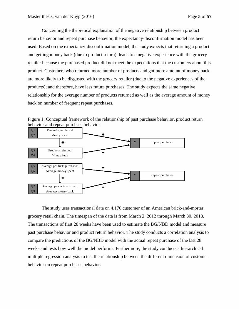
Below, Figure 1 examines the conceptual framework of the relationship between past
purchase behavior as well as product return behavior and repeat purchase behavior. The
theoretical explanation on the positive relationship between past purchase behavior and repeat
purchase behavior holds that, customers who purchased more number of products as well as
customers who spent more amount of money are the customers who visited the store more
frequently. Following, customers who visited the store more frequently have a stronger
relationship with the grocery retailer and are therefore more likely to continue their purchase
habits in the future. In addition, the study uses the same explanation on the negative relationship
between the average number of products purchased as well as average amount of money spent on
number of frequent repeat purchases. It assumes that customers who purchased on average less
number of products per visit and spent on average less amount of money per visit, are the
customers who visited the store more frequently. They visited the store more frequently because
they spread their grocery expenses across multiple visits instead of buying all their groceries in
just a few visits. In line with this reasoning, the study expects that customers who purchased on
average less number of products and who spent on average less amount of money, tend to have
stronger relationship and continue their purchases habits in the future; resulting in a higher
number of frequent repeat purchases.
Master thesis, van der Kuyp (2016) Page 5 of 57
Concerning the theoretical explanation of the negative relationship between product
return behavior and repeat purchase behavior, the expectancy-disconfirmation model has been
used. Based on the expectancy-disconfirmation model, the study expects that returning a product
and getting money back (due to product return), leads to a negative experience with the grocery
retailer because the purchased product did not meet the expectations that the customers about this
product. Customers who returned more number of products and got more amount of money back
are more likely to be disgusted with the grocery retailer (due to the negative experiences of the
products); and therefore, have less future purchases. The study expects the same negative
relationship for the average number of products returned as well as the average amount of money
back on number of frequent repeat purchases.
Figure 1: Conceptual framework of the relationship of past purchase behavior, product return
behavior and repeat purchase behavior
The study uses transactional data on 4.170 customer of an American brick-and-mortar
grocery retail chain. The timespan of the data is from March 2, 2012 through March 30, 2013.
The transactions of first 28 weeks have been used to estimate the BG/NBD model and measure
past purchase behavior and product return behavior. The study conducts a correlation analysis to
compare the predictions of the BG/NBD model with the actual repeat purchase of the last 28
weeks and tests how well the model performs. Furthermore, the study conducts a hierarchical
multiple regression analysis to test the relationship between the different dimension of customer
behavior on repeat purchases behavior.

Master thesis, van der Kuyp (2016) Page 6 of 57
The structure of the chapters is as follows. To start, chapter 2 gives an overview of the
literature that focuses on the prediction of repeat purchase behavior. Following, chapter 3
discusses the theoretical background, which have been used to formulate 8 different hypotheses.
Further, chapter 4 presents the research design of this study. Next, in chapter 5, the study
overviews the results of the correlation analysis and the hierarchical multiple regression analysis.
Chapter 6 gives a discussion on the theoretical background, the research design and the findings
of the study. Lastly, chapter 7 presents the conclusion by reviewing the main results and finding
of this study. Additional Tables, Figures and the syntax can be found in the appendix.
Master thesis, van der Kuyp (2016) Page 7 of 57
II. Literature review
Entering the digital-age, the business environment and the way business interact with
their customers has dramatically changed. Developments in database technology have made it
possible for businesses to capture large amounts of customer data; and in return the data is used
to get customer insights. Concepts of relationship equity, customer retention and customer repeat
purchases have been widely discussed within the marketing literature (Slater & Narver, 1998;
Vesanen & Raulas, 2006; Arons, van den Driest, & Weed, 2014; Avery, Fournier, &
Wittenbraker, 2014). Further, the research agenda of the Marketing Science Institute 2014-2016
prioritizes on developing marketing analytics for a data-rich environment and getting customer
deep-insight”. In response, academics and practitioners have paid enormous attention on
predicting repeat purchases behavior; using advanced statistical models on past purchases
behavior.
In the literature that focuses on predicting repeat purchase behavior, theoretical work
mostly takes on a more data-driven approach; and its focus is largely on the application of several
techniques on customers’ purchases. Repeat purchases have been the object of research for many
years. Starting at the 1950s mass marketing techniques of mail orders like catalogs have been
used to communicate and collect data on customers. This has dramatically changed after the
1960s when computers were introduced and marketers started using customer loyalty cards to
collect extensive amount of customer data. Prepackaged statistical programs SAS and SPSS has
also allowed marketers to analyze the customer data and build models for customer behavior
(Petrison, Blattberg, & Wang, 1997; Stone & Shaw, 1988).
To describe and predict repeat purchases of customers in a non-contractual setting,
(Schmittlein, Morrison, & Colombo, 1987) developed the Pareto/NBD model. The setting is
characterized with unobservable dropout behavior and high customer heterogeneity in number of
purchases. “The model assumes that customers buy at a steady rate for a certain period of time
and then become inactive” (Fader et al., 2005). It uses two different levels to estimate parameter
of “purchase rate” and “dropout rate”. The number of repeat purchases is modeled using the NBD
(negative binominal distribution) (poising-gamma mixture counting) model; and the customer
dropout is modeled using the Pareto (exponential-gamma mixture). To make predictions on
repeat purchases, the model requires transaction history information on the number of past
purchases and the recency of the last purchase.

Master thesis, van der Kuyp (2016) Page 8 of 57
Since its development, several studies have showed its strength in predicting repeat
purchases (Fader et al., 2005; Reinartz & Kumar, 2000). Wübben & Wangenheim (2008)
compare the different techniques which will provide a better understanding of their application.
In their study the effectiveness of the simple heuristic model is tested against two stochastic
models, the BG/NBD and Pareto/NBD. Results show that the stochastic models perform better
than the heuristic model on predicting repeated purchases.
However, despite the wide interest of academics in modelling customer behavior,
marketers have failed to the Pareto/NBD model due to its complicated estimation procedure that
incorporates various evaluation of Gaussian hyper-geometric function. Verhoef, Spring, Hoekstra
& Leefland (2003) test the usages of the statistical models in businesses; and find that most of the
businesses still use heuristic methods cross-tabulation and RFM model on predictive analysis
instead of more advanced methods like the Pareto/NBD model. The authors show importance of
fit between business practices and academic research and that researchers should consider the
applicability of new techniques (Verhoef, Spring, Hoekstra, & Leeflang, 2003)
In response, academics have tried to develop statistical techniques which are faster and
easier to implement. Fader & Hardie (2001) use transaction data from an online context of CD
purchases to predict future transactions and sales. The authors use a simplified stochastic model,
which can be implemented using spreadsheet software. The study shows how past purchases can
be used to predict future sales (Fader & Hardie, 2001).
Following, a few years later, Fader et al. (2005) have developed the BG/NBD model. The
model is almost identical as the Pareto/NBD model, except that it assumes that customer dropout
occurs only after a customer purchases. Instead of using a Pareto (exponential-gamma mixture) it
uses a beta-geometric model. Due to this slight variation, the model is implemented way faster
and easier. Whereas the Pareto/NBD model needs advanced computation software like MATLAB
to estimate its parameters; the BG/NBD model can be implemented with spreadsheet software
and is therefore more accessible for businesses. Results show that the predictions of the
Pareto/NBD and the BG/NBD are almost the same (Fader et al., 2005; Wübben & Wangenheim,
2008).
In testing the relationship between past purchase behavior and future customer
purchasing, academic studies find that the amount of money customers spent forms a good
predictor of repeat purchases. Reinartz & Kumar (2000) uses data on online catalog company and
Master thesis, van der Kuyp (2016) Page 9 of 57
find a positive relationship between customer profitability and customer lifetime value. Further
Cheng & Chen (2009) uses a RFM model to predict repeat purchases. Again, the results show
that the amount of money customers spent is a good predictor for repeat purchases.
This study extends previous studies on the relationship between past purchase behavior
and repeat purchases by including product return behavior. Literature on product return behavior
focusses mostly on Ready Made Garments and the related clothing industry and not so much on
brick-and-mortar grocery retailing. This is because it is quite common to return cloths whereas
grocery products are only returned when the quality of the purchased product is insufficient.
Related studies at this setting focusses mostly on relationship between satisfaction and customer
return (Anderson & Mittal, 2000; Verhoef, 2003). The relationship between product return
behavior and future purchases using transaction data has not been studied. Moreover, we find
limited application of the BG/NBD model in brick-and-mortar grocery retail setting. This study
therefore validates the BG/NBD model at a brick-and-mortar grocery retail setting; and tests the
relationship between past purchase behavior and repeat purchase behavior including product
return behavior. The following research question is answered:
Which dimensions of customer behavior in a brick-and-mortar retailing setting predict the repeat
purchases the best?
Academic and managerial contributions
Predicting customer future purchases at brick-and-mortar grocery retailing, the study adds
knowledge about the empirical validation of the BG/NBD model. As mentioned, the used dataset
contains a big group of people with extreme number of frequent visits on short interval which
could violate certain purchase behavior assumptions of the model. By validating the model, the
study finds if the model performs well enough on this particular data. Further, its empirical
validation can be compared with previous studies that validate the BG/NB on a different setting.
Fader et al (2005) use transaction data on customer of an online CD company and find a
correlation of (r =0,626, p = 0,000) between the predict repeat purchases and the actual repeat
purchases. To draw further conclusion whether this correlation is good predictor, both studies are
compared with each other. Managers from different settings can use this study to decide whether
the apply the model.
Master thesis, van der Kuyp (2016) Page 10 of 57
Moreover, the study extends previous studies on past purchase behavior by including
product return behavior. Product return behavior is not so much studied in a brick-and-mortar
retail setting. The results of this study provide varies insights for academics and managers on the
importance of product returns. To start, results give the mangers insights on the amount of
product returns in brick-and-mortar grocery retailing. Using a large amount of data, indications
can be given on how many products customers return in respect to the number of products they
purchase.
Further, the study tests the relationship between past purchases as well as product return
behavior and repeat purchase behavior. It thereby adds knowledge on the different dimension of
customer behavior that predict future purchases. Moreover, results provide grocery retail
managers insight in the effects that product defects and the related product returns have on future
sales. The results could help managers to think about the implications that product defects have
and further they can be used to adjust current product return policies.
At last, basic probabilistic customer-base analysis can be improved with the results of this
study. The current BG/NBD model uses only purchase history on frequency of purchase and
recency of last purchase. However, the model can be improved when covariates are layered into
the model. In our purpose of finding predictors of repeat purchases, the dimensions which predict
repeat purchases the best can be used to improve the model. For instance, a covariate of product
return behavior could be used to improve predictions of the BG/NBD model.
Master thesis, van der Kuyp (2016) Page 11 of 57
III. Theoretical background
Theories on past purchase behavior and product return behavior
This section presents the theories on the relationship between the past purchase behavior
as well as the product return behavior and the future repeat purchases in a brick and mortar
grocery retailing. First it discusses the relationship between past purchase behavior and repeat
purchases and thereafter the relationship between product return behavior and repeat purchases.
Past purchase behavior. Starting with the former, academic studies indicate that past
purchase behavior form a good predictor for repeat purchase behavior (Dwyer et al., 1987;
Reichheld & Teal, 2001; Reinartz & Kumar, 2003; Cheng & Chen, 2009). This is because
customers who visited the store more frequently, have a stronger relationship with the store; and
customer who have stronger relationship with the store are likely to maintain their repeat
purchases habits in the following period. Following, the number of frequent visits is associated
with the number of products purchased and amount of money spent. Customer who visited the
store more frequent also purchased more number of products and spent more amount of money at
this store. They have a stronger relationship with the store than customers who visited the store
less frequent; and therefore have more future purchases. Therefore, the study expects that:
H1: Customers who have purchased more number of products during a fixed period of time, have
a higher number of frequent repeat purchases.
H2: Customer who have spent more amount of money during a fixed period of time, have a
higher number of frequent repeat purchases2.
Following, the number of frequent visits and repeat purchases is associated with average
number of products purchased and the average amount of money spent per visit. Customers that
visited the store more frequently are the customers that purchased less number of products and
spent less amount of money per visit. They spread their grocery expenses across multiple visits
instead of buying all their groceries at one visit and therefore visited the store more frequently. In
2 The numbers of the hypotheses correspond to the numbers of the sub-questions. H1 (the relationship between
products purchased and repeat purchases) corresponds to Q1, H2 (the relationship between money spent and repeat
purchases) corresponds to Q2, etc.
Master thesis, van der Kuyp (2016) Page 12 of 57
addition, they have a stronger relationship with the store and are likely to continue their purchase
habits in the future. This study expects that:
H5: Customers who purchased on average less number of products per visit, have a higher
number of repeat purchases.
H6: Customers who spent on average less amount of money per visit, have a higher number of
frequent purchases.
Product return behavior. If the quality of the product is insufficient customers can
return their product(s) and get their money back. This study focuses on both types of product
return behavior: the number of products returned and the amount of money back (due to product
return). Since product return behavior has not been studied so much for brick-and-mortar grocery
retailing chains, the study proposes three different types of reasoning on the relationship between
product return behavior on repeat purchase behavior.
The first stream of reasoning holds that the product return behavior of customers at brick-
and-mortar grocery retailing is irrelevant for predicting the number of frequent repeat purchases.
To start, its relationship with repeat purchases is irrelevant because returning products at brick-
and-mortar grocery retailing rarely takes place3. At the brick-and-mortar grocery retailing
customers return the purchased product when it is broken or the quality is insufficient. The
product return policies are stricter in comparison to the clothing industry, where firms offer
generous product return policies of 10 till 30 days after the purchase. Because customers rarely
return a product the relationship between product return behavior and repeat purchases is
irrelevant.
Secondly, if there is a relationship between the number of products customers returned
and number of frequent repeat purchases, this relationship is spurious. To return a product
customer first need to purchase that product. Customers who purchase more products are more
likely to return a product (compared to customers who purchase less products) they are more
likely to buy a defected product. The relationship between the number of products purchased and
3 According to this study around 0.1% of the total purchases is returned.

Master thesis, van der Kuyp (2016) Page 13 of 57
number of frequent repeat purchases is therefore a logical outcome of the number of products that
the customer purchases.
Thirdly, if product return behavior influences customers’ satisfaction with the grocery
retailer brick-and-mortar grocery retailing, this will not lead to dropout behavior. In studying the
relationship between customer satisfaction and customer switching behavior, (Anderson &
Mittal, 2000) find that dissatisfaction doesn’t necessary lead to dropout behavior. Customers can
be dissatisfied but still remain shopping at the same store, and vice versa, be satisfied but switch
to the competitor. It shows that purchase habits are more important that the satisfaction with the
grocery retailer and therefore the affective change related to product return behavior are
irrelevant for future purchases (Dick & Basu, 1994; Keaveney, 1995). Therefore, in line with the
argumentation the null hypothesis is expects that:
H03: the number of frequent repeat purchases doesn’t differ if customers have returned more or
less number of products during a fixed period
H04: the number of frequent repeat purchases doesn’t differ if customers have got more or less
amount of money back (due to returning a product) during a fixed period
In contrast, according to expectancy-confirmation model, customers hold certain
expectations about the products and if the expectation are not met, the likelihood of customer
disgust increases (Oliver, 1980; Alexander, 2012). Returning a product lead to with customer
disgust when the initial expectations about the product _are not met buy the outcome of the
product. Disgust is a function of the negative affect (grief) plus a negative surprise (Alexander,
2012). Again returning a product causes negative affect or negative surprise because the outcome
of the product doesn’t meet the initial expectation of the product. For instance, when the date of
the milk has expired, the customer experiences grief because he has to return the product and
cannot drink it right away. His expectations about the milk didn’t meet the outcome of the milk.
Customer who returned more number of products and got more money back are more likely to be
disgusted they experience have more negative experience with the grocery retailer. The
alternative hypothesis therefore expects that:
Master thesis, van der Kuyp (2016) Page 14 of 57
Ha3: the more number of products customers returned during a fixed period of time, the lower
number of frequent repeat purchases
Ha4: the more amount of money customers got back per visit (due to returning a product) during
a fixed period of time, the lower number of frequent repeat purchases
As mentioned, product return behavior takes rarely place at brick-and-mortar grocery
retailing. The study expects same negative relationship between the average product return
behavior per visit and number of frequent repeat purchases, namely that:
H07: the number of frequent repeat purchases doesn’t differ if customers returned on average
more number of products per visit.
H08: the number of frequent repeat purchases doesn’t differ if customers got on average more or
less amount of money back (due to returning a product) per visit.
Ha7: customer who returned on average more number of products per visit, have less number of
frequent repeat purchases
Ha8: customers who got on average more amount of money back per visit (due to returning a
product), have less number of frequent repeat purchases
Alternatively, the third line of reasoning holds that product return behavior leads to
delight instead of disgust. According to Alexander (2012), delight as a function of the positive
affect ‘joy’ and positive surprise. Customer expectations are formed by previous experiences
together with social norms. In brick-and-mortar grocery retailing absence on product return
behavior lowers customer expectations on returning a product. If customers got their money back
(due to returning a product), this outcome overestimate their its initial expectations on returning
the product leading to a positive surprise (Alexander, 2012). Assuming that customers who
returned products enjoy a positive surprise and thus are more delighted than those who don’t

Master thesis, van der Kuyp (2016) Page 15 of 57
return products. The third stream of reasoning expects therefore that higher product return
behavior lead to higher repeat purchases behavior.
Since product return is mostly the results of insufficient quality, it is not likely that
customers will have a positive experience by returning their products. Therefore, the study holds
no hypothesis on the third line of reasoning.

Master thesis, van der Kuyp (2016) Page 16 of 57
IV. Research design
Data
To provide an answer on the research question this study uses the “Acquire Valued
Shoppers” (AVS) challenge data of Kaggle4. Kaggle is an open source platform that provides the
link between data problems and data solutions. Users of the platform come from all over the
world. They form the largest community of data scientists consisting of tens of thousands PhD’s
in quantitative fields (e.g. computer science, statistics, econometrics, math and physics). Data is
publically available to all scientists for the purpose of the competition5. The scientists finding the
best solution to solve the complex data science problems get a determined amount of prize
money. In return the company with the data problem or sponsor pays a certain amount of fee.
Academics have the possibility to work in teams and use forums to share issues and results6.
The ASV data was collected by 134 brick-and-mortar grocery retailers which are located
at 34 different geographical regions. In total, 350 million transactions were recorded of 311.541
customers. Each store chain recorded all the transactions of each shopping cart during a period of
coupon promotion. Customers that redeemed the coupon offer were selected for the data. All
purchase information on customer and product were anonymized to protect customers and sales
information. Names of customers, brands, companies and store chain are replaced by unique
identification numbers that correspond to the names. The original purpose of the challenge was to
find the best solution of predicting which shopper will become repeat buyers of the product of the
coupon offer. However, the transaction information can be used for different research purposes.
This study uses the transaction information to measure how many products customers
purchased or returned; and to measure the amount of money customers spent or got back (due to
product return). Following, it purposes to find the dimensions of customer behavior that predict
the number of frequent repeat purchases the best. Table 1 describes the key variables of the initial
dataset, which have been used to construct the different dimension of customer behavior.
4 See https://www.kaggle.com/c/acquire-valued-shoppers-challenge/data for the information on the data and to find
the data. 5 Kaggle stated that it is not responsible for the credibility of the data. To increase the validity, strong effort was
taken in cleaning the data before using it for analysis (Saunders, Lewis, & Thornhill, 2009) 325-331). Further,
inaccurate records have been reported in the appendix. 6See the Kaggle forums https://www.kaggle.com/c/acquire-valued-shoppers-challenge/forums for appropriate
discussion of the administrators and the participants on the data
Master thesis, van der Kuyp (2016) Page 17 of 57
To answer the research question, the grocery retailer with the highest number of
customers has been selected. Since all purchase information has been anonymized there is no
additional information on this grocery retailer expect the overall statistics of customer purchases7.
The retailer has transaction information on 32.640 customers and the timespan of their
transactions ranges from March 2, 2012 through July 23, 2013. The store offers a wide selection
of products from over 25.000 different brands. Most of the products that are sold have the price
between $0,50 and $5, - dollar but also products with a price of $10, - dollar or higher are sold.
Remarkable, is that the retailer collected an extensive amount of data over a period of almost one
and a half year. During this period the shopping cart information of over 3 million visits, with an
average around 92 visit per customers, have been traced. It is assumed that the company uses
memberships cards and that customers need to scan their card each time they visit the store.
From the initial 32.640 customers, a sample of 4.208 customers (with 5.669.001
transactions) has been used. The final dataset contains all customers that made their “first
purchase” during March and April 2012. In the study 38 customers who made their first purchase
after April 30, 2012 have been removed because they are from a different customer cohort. The
remaining sample of this study contains 4.170 customers8. Further the timespan of the
transactions has been adjusted from “March 2, 2012 through July 23, 2012” to “March 2, 2012
through March 30, 2013” because most of the transactions after March 30, 2013 were not traced9.
The adjusted dataset has been used to create two time periods of 28 weeks: the calibration period
and validation period. The calibration period ranges from March 2, 2012 through September 14,
2012 and the validation period from September 15, 2012 through March 30, 2012. With the
calibration period the variables of the past purchase behavior and product return behavior have
been calculated. The past purchase behavior has been used to construct the BG/NBD model and
predict the number of frequent repeat purchases. With the validation period the actual repeat
purchases have been calculated.
7 See Table in the appendix for additional statistics on the grocery retail 8 The selection of the customers with the same cohort is based on the study of Fader et al (2005). The authors select
the customers who made their first purchase during the first quarters, whereby the full dataset contains of five
quarters. This study selects the customers who made their first purchase during the first two months, whereby the full
dataset contains 13 months. 9 See Figures in the appendix for the customer activity from March 2, 2012 through July 23, 2013. The customer
activity measures the number of visits per day at the studied grocery retailer. On average between 900 and 1200
customers visit the grocery retailer per day. From March 30, 2013 the customer activity decreases every day. The
same decrease has been found for other grocery retailers in the Acquire Valued Shopper dataset. The study expects
the grocery retailers didn’t provide the full transaction data from March 30. 2013 and therefore adjusts the timespan.
Master thesis, van der Kuyp (2016) Page 18 of 57
To assess the applicability of the data, the study discusses the advantages and
disadvantages of the final dataset. Starting with the advantages, the used dataset is applicable for
empirical validation of the BG/NBD model. The calibration period can be used to build the
model and the validation period can be used to test how well the models performs in respect to
the actual number of frequent repeat purchases.
Furthermore, the key variables of the initial dataset (see Table 1) can be used to construct
the different dimension of customer behavior and measure repeat purchases. The transactions
contain not only information on the number of products purchased (purchase_quantity positive)
and amount of money spent (purchase_amount positive) but also information on the number of
products returned (purchase_quantity negative) and the money of money customers got back due
to returning the products (purchase_amount negative). Therefore, the transaction information can
be used to measure different dimensions of past purchase behavior as well as product return
behavior. In addition, the BG/NBD model requires information on the numbers of purchases
(frequency of buying) and recency of last purchase (recency). The transaction information on the
date of transaction (date) can be used to calculate the both the frequency of buying and recency.
On the other hand, the used data also holds multiple disadvantages. To start, there is no
description on the brick-and-mortar grocery retailer and whether it concerns a non-contractual
setting or a contractual setting remains unknown. As mentioned, Kaggle anonymized the
transaction data and therefore it is unknown what products the grocery retailer sold. Further, it is
also unknown how the company collected this large amount of transaction data. The study
assumes that the retailer uses some kind of membership card whereby each time a customer visits
the grocery retailer he uses the card to register his purchases. Yet, this is an assumption which we
cannot be certain about. Following from this assumption, it remains unknown whether the
customers have a contract with the retailer or not. If the customers have a contract and pay a
certain amount of membership fee, the results only apply to brick-and-mortar grocery retailers in
a contractual setting. Academic studies find differences in customer behavior in contractual
setting or non-contractual (Tsai, Huang, Jaw, & Chen, 2006; Woisetschläger, Lentz, &
Evanschitzky, 2011)10. Thus, the results of this study could have been influenced by the setting
of the data.
10 See chapter 6 for further discussion on the dataset

Master thesis, van der Kuyp (2016) Page 19 of 57
Further, there could be a selection bias in the data. As mentioned, the grocery retailers
collected the data on customers who were selected for a coupon promotion and who redeemed the
coupon. No additional information is given on how the customers were selected. It could be that
customers were selected because of previous purchases. In this case the data is biased towards
customers with a certain previous purchase behavior. Moreover, the study also doesn’t know if
customers who did redeem the coupon differ in behavior from customers who didn’t redeem the
coupon. If so, the purchase behaviors in the data are biased as well.
At last, the used data contains some systematic measurement errors. As mentioned, the
timespan of the final dataset has been adjusted because the data stops tracing most of the
transactions after May 30, 2013. The transactions after May 2013 can therefore not been used for
this study. Further, doing some descriptive analysis on the key variables of Table 1, the study
finds that 0.34% of all transactions misses information on the number of products purchased
(purchase_quantity positive), the amount of money spent (purchase_amount positive), the
number of products purchased (purchase_quantity negative) and the amount of money back
(purchase_amount negative). The study expects that the missing information didn’t influence the
results. According to the statement on Kaggle’s website, it is common to find some noise in real-
world data (A Note On Data Quality, 2013). Furthermore, the study finds that the noise is spread
across different customers and not concentrated on the transaction of only a few customers
Table 1: Key variables of original dataset
Variable Description Range
id Unique number representing the customer [1 – 32.640]
chain Unique number representing the store chain [21]
date Date of transaction [2012 03-02 –
2013 07 30]
Purchase_quantity positive Number of products purchased per transaction [0 – 95]
Purchase_quantity negative Number of products returned per transaction [0 – 50]
Purchase_amount positive Amount of money spent per transaction [0 – 1.200]
Purchase_amount negative Amount of money returned per transaction [0 – 100]
Considering the advantages and disadvantages, the study concludes that the used dataset
is applicable to answer the research question. Although there is no additional information on the
grocery retailer and the data contains some systematic measurement errors; the data is applicable
Master thesis, van der Kuyp (2016) Page 20 of 57
to measure different dimension of customer behavior and repeat purchases behavior and
statistically test the relationship between past purchase behavior as well as product return
behavior and repeat purchase behavior. In this way it can find the best predictor of repeat
purchases and answer the research question.
Key variables
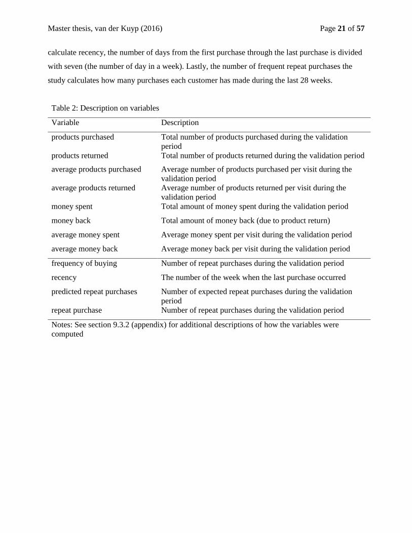
The key variables have been computed using the spreadsheet software Excel. In this
section the computation of the variables is discussed along with some descriptive statistics of the
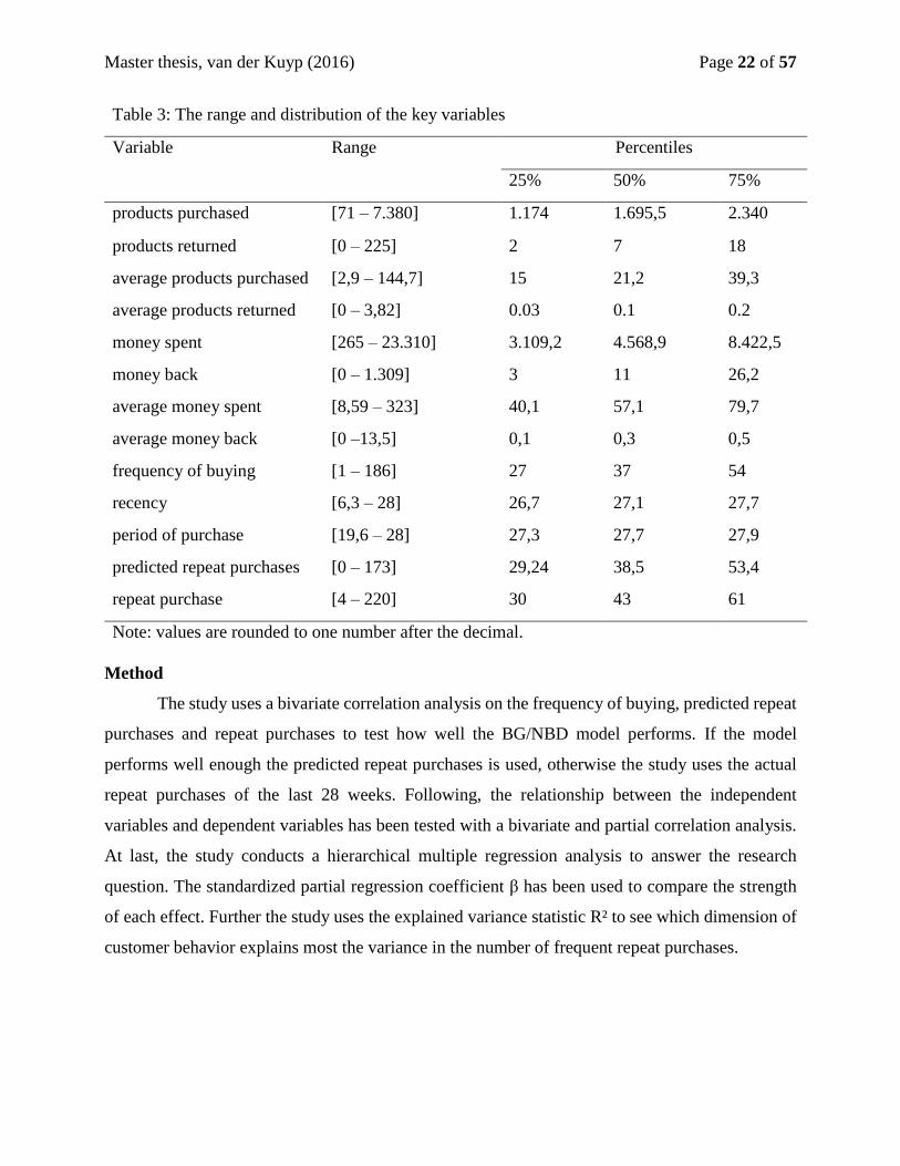
variables. Table 2 gives the definitions of the key variables and Table 3 provides its range and
distribution. For a detailed description of the formulas that have been used to compute the key
variables, see the variable computation in the appendix.
Past purchase behavior and product return behavior. As discussed, the initial dataset
contains information on the transaction level. For the purpose of this research, the transaction
level data has been transformed to customer level data. Firstly, the transactions that occurred on
the same day have been added up to calculate the total sum of purchases per visit for each
customer. The study uses “purchase_quantity positive” and “purchase_quantity negative” to
calculate how many number of products the customers purchased per visit and how many number
of products the customers returned per visit. Further, “purchase_amount positive” and
“purchase_amount negative” have been used to calculate the amount of money the customers
spent per visit and the amount of money the customers got back (due to product return) per visit.
Secondly, the study uses the sum of all purchases during the first 28 weeks, to calculate “the
number of products purchased”, “the amount of money spent”, “the number of products returned”
and “amount of money back”. Following, the study calculated the average of the four variables to
compute “the average number of products purchased”, “the average amount of money spent”,
“the average number of products purchased” and “the average amount of money back”.
Predicted repeat purchases and repeat purchases. The BG/NBD model has been used
to predict the number of frequent repeat purchases. The model requires two types of information
namely the number of frequent purchases and the recency of the last purchase. Again, the
transactions occurred on the same day were added up. Following, the study calculated how many
purchases each customers has during the first 28 weeks. This variable is called the “frequency of
buying”. Recency is the number of the week of the last purchase during the first weeks. To
Master thesis, van der Kuyp (2016) Page 21 of 57
calculate recency, the number of days from the first purchase through the last purchase is divided
with seven (the number of day in a week). Lastly, the number of frequent repeat purchases the
study calculates how many purchases each customer has made during the last 28 weeks.
Table 2: Description on variables
Variable Description
products purchased Total number of products purchased during the validation
period
products returned Total number of products returned during the validation period
average products purchased Average number of products purchased per visit during the
validation period
average products returned Average number of products returned per visit during the
validation period
money spent Total amount of money spent during the validation period
money back Total amount of money back (due to product return)
average money spent Average money spent per visit during the validation period
average money back Average money back per visit during the validation period
frequency of buying Number of repeat purchases during the validation period
recency The number of the week when the last purchase occurred
predicted repeat purchases Number of expected repeat purchases during the validation
period
repeat purchase Number of repeat purchases during the validation period
Notes: See section 9.3.2 (appendix) for additional descriptions of how the variables were
computed
Master thesis, van der Kuyp (2016) Page 22 of 57
Table 3: The range and distribution of the key variables
Variable Range Percentiles
25% 50% 75%
products purchased [71 – 7.380] 1.174 1.695,5 2.340
products returned [0 – 225] 2 7 18
average products purchased [2,9 – 144,7] 15 21,2 39,3
average products returned [0 – 3,82] 0.03 0.1 0.2
money spent [265 – 23.310] 3.109,2 4.568,9 8.422,5
money back [0 – 1.309] 3 11 26,2
average money spent [8,59 – 323] 40,1 57,1 79,7
average money back [0 –13,5] 0,1 0,3 0,5
frequency of buying [1 – 186] 27 37 54
recency [6,3 – 28] 26,7 27,1 27,7
period of purchase [19,6 – 28] 27,3 27,7 27,9
predicted repeat purchases [0 – 173] 29,24 38,5 53,4
repeat purchase [4 – 220] 30 43 61
Note: values are rounded to one number after the decimal.
Method
The study uses a bivariate correlation analysis on the frequency of buying, predicted repeat
purchases and repeat purchases to test how well the BG/NBD model performs. If the model
performs well enough the predicted repeat purchases is used, otherwise the study uses the actual
repeat purchases of the last 28 weeks. Following, the relationship between the independent
variables and dependent variables has been tested with a bivariate and partial correlation analysis.
At last, the study conducts a hierarchical multiple regression analysis to answer the research
question. The standardized partial regression coefficient β has been used to compare the strength
of each effect. Further the study uses the explained variance statistic R² to see which dimension of
customer behavior explains most the variance in the number of frequent repeat purchases.
Master thesis, van der Kuyp (2016) Page 23 of 57
V. Results
To answer the research question, the study tests the relationship between past purchase
behavior as well as product return behavior and number of frequent repeat purchases. The section
has been divided in the preliminary analysis and the explanatory analysis. The preliminary
analysis tests the predictive accuracy of the BG/NBD model and measures a bivariate correlation
between the independent and dependent variables. The explanatory analysis uses partial
correlation analyses and hierarchical multiple regression analyses to test which dimension of
customer behavior predicts repeat purchases the best. The regression analyses use the
standardized (partial) regression coefficient β to compare the different effects; and the explained
variance statistics R² to find the best predictor of repeat purchases.
Preliminary analysis
Firstly, to assess the predictive accuracy of the BG/NBD model, a bivariate correlation
between frequency of buying, predicted repeat purchases and repeat purchases has been used. If
the model predicts well enough the study uses the predicted repeat purchases to test its
relationship with past purchase behavior and product return behavior. The results of the bivariate
correlation between frequency of buying predicted repeat purchases and repeat purchases have
been examined in Table 3. The study finds a high and positive correlation of (r = 0,999, p =
0,000) between frequency of buying and predicted repeat purchases. The strong correlation
shows that the number of frequent repeat purchases predicted by the BG/NBD model are almost
identical to the frequency of buying. Surprisingly, correlation between frequency of buying and
repeat purchases is larger than the correlation between predicted repeat purchases and repeat
purchases. The correlation of frequency of buying and repeat purchases is (r = 0,864, p = 0,000)
while the correlation of predicted repeat purchases and repeat purchases is (r = 0,864, p = 0,000).
This analysis shows that the BG/NBD model performs less well the frequency of buying in
predicting repeat purchases.

Master thesis, van der Kuyp (2016) Page 24 of 57
Table 3: Bivariate correlations repeat purchases, predicted repeat purchases and frequency
of buying
Bivariate correlations
(1) (2) (3)
(1) Repeat purchases 1
(2) Predicted repeat purchases 0,864 1
(0,000)
(3) Frequency of buying 0,864 0,999 1
(0,000) (0,000)
In addition, it has been visualized how well the model performs across customers with the
same level of frequency of buying. In Figure 2, the horizontal axis shows the frequency of
buying. Further, the vertical axis shows the average numbers of predicted repeat purchases and
the average number of repeat purchases for the customers with the same frequency of buying.
Looking at both lines, the average predicted repeat purchases and the average repeat purchases
are almost the same for customers with a low frequency of buying. Further, when the frequency
of buying increases, the average predicted repeat purchases and repeat purchases deviate from
each other. The increase in deviation shows that the average predictions of the BG/NBD model
are more accurate for customers with a low frequency of buying; and that the predictions of the
model get less accurate when the frequency of buying increases. The deviation between the
predicted repeat purchases and repeat purchases are likely to be a results of the assumptions that
the BG/NBD model holds. Our dataset is characterized with extreme frequent visit on short
interval and therefore it is likely that the assumptions have been violated using this particular
data.
Figure 2: The average number of predicted repeat purchases versus repeat purchases per level of
frequency of buying
Master thesis, van der Kuyp (2016) Page 25 of 57
At last, the study compares the correlation results with the CDNOW dataset of Fader et al
(2005). In this study, the authors test how well it performs the BG/NBD model performs in
relation to the Pareto/NBD model in predicting repeat purchases. Using the CDNOW data, the
relationship between predicted repeat purchases and repeat purchases finds the following
correlation of (r =0,626, p = 0,000). Further the correlation between frequency of buying and
repeat purchases of (r = 0,557, p = 0,000) has been found. Both correlations are weaker than the
correlations of the previous analysis, which show that past purchase behavior in brick-and-mortar
grocery retailing predicts the number of frequent repeat purchases better than the customer
purchase-behavior at online-CD retailing. However, the BG/NBD model did improve predictions
in respect to frequency of buying using the CDNOW data. The correlation increases from r =
0,557 to r =0,626, while the correlation on this particular data decreases from r = 0,864 to =
0,864. Because the BG/NBD model didn’t perform well enough on this data, it has been decided
to use number of actual repeat purchases of the validation period for the final analysis instead of
the predictions of the BG/NBD model. It uses a better measurement of repeat purchases and
thereby increases the interval validity of this study.
Furthermore, the study tests the correlation between customers purchase behavior as well
as product return behavior and repeat purchases. It has been assumed that both the number of
products purchased and amount of money spent have a positive correlation with repeat purchases;
and that the number of products returned and amount of money back (due to product return) both
have a negative correlation with repeat purchases.
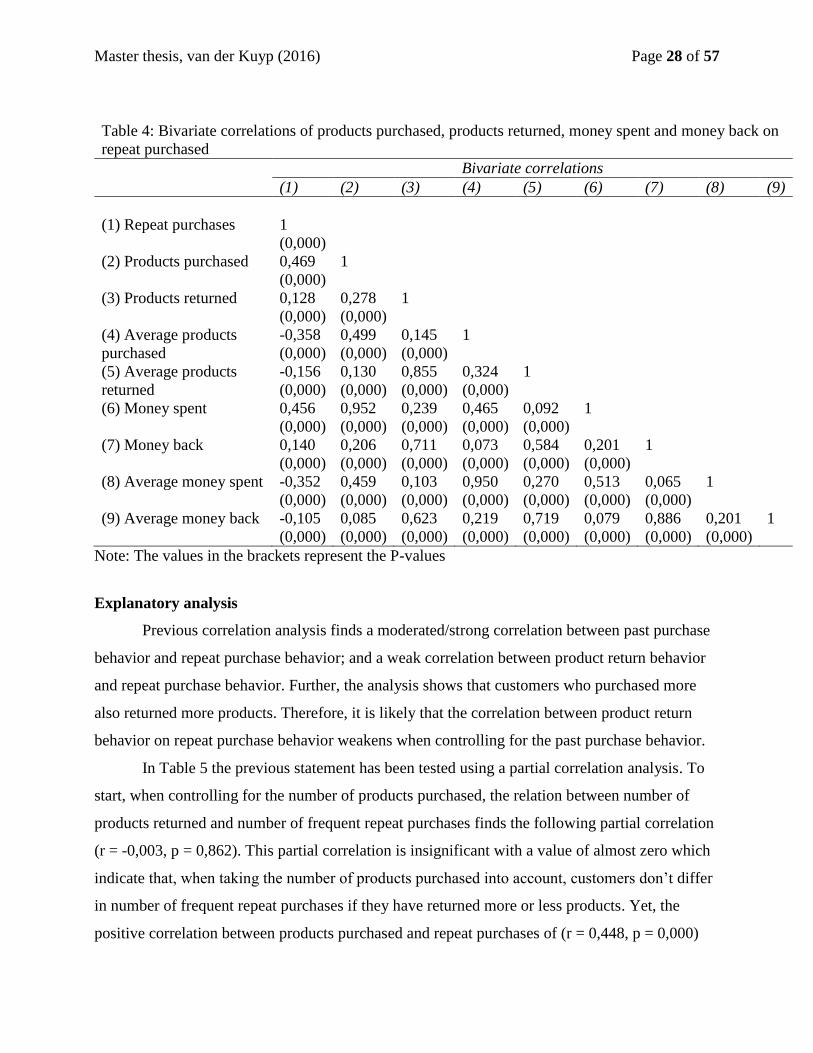
Table 4 examines the results of the correlation analysis on the independent and dependent
variables. To start, products purchased has a correlation of (r = 0,469, p = 0,000) with repeat
purchases and money spent has a correlation of (r = 0,456, p = 0,000). This shows that customers
who purchased more number of products and spent more amount of money, have a higher
number of frequent repeat purchases.
Following, as expected, a negative correlation has been found for average number of
products purchased and average amount of money spent on the number of frequent repeat
purchases. The customers who purchase on average less products per visit and spend on average
less money per visit are the customers who visit the store more frequent. Therefore, customer
who purchased on average less number of product and spent on average less amount of money
has a higher the number of frequent repeat purchases. The relationship between average number

Master thesis, van der Kuyp (2016) Page 26 of 57
of products purchased and repeat purchases is (r = -0,358, p = 0,000); and the correlation between
average amount of money spent on repeat purchases is (r = -0,353, p = 0,000). Comparing both
correlations with “number of products purchased” and “amount of money spent”, the “average
number of products purchased” and “average amount of money spent” have a weaker correlation
with repeat purchase.
Focusing on product return behavior, the number of products returned has a correlation of
(r = 0,128, p = 0,000) on repeat purchases and amount of money back (due to product return) a
positive correlation of (r = 0,140, p = 0,000). Finding a positive correlation on both variables is
surprisingly, since the study expects that customers who return more number of products and got
back money amount of money (due to product return) have a lower number of frequent repeat
purchases. The positive correlation is in line with third reasoning of the relationship between
product return behavior and repeat purchases; it holds that customers who return more products
and get more money back are more delighted and therefore more often come back.
Yet, it could be that customers who return more number of products also purchased more
products and therefore have a higher number of frequent repeat purchases. Taking into account
the number of visits, the relationship between average number of products returned and repeat
purchases has a correlation of (p = -0,156, p = 0,000). Further the relationship between average
amount of money back (due to product return) and repeat purchases has the correlation of (r = -
0,105, p = 0,000). Finding a negative correlation confirms the assumption that customers who
return on average more products and get on average more money back (due to product return) are
more likely to be disgusted with the grocery retailing and therefore have a lower number of
frequent repeat purchases. Nevertheless, respective of its direction, the variables “products
returned”, “money back” and “average products returned” and “average money back”, all have
correlation of below r = 0,17 on repeat purchases. Given the fact that the variables “products
purchased”, “money spent”, “average products purchased” and “average money spent” all have a
strong correlation with repeat purchases it is likely to expect that the relationship between
product return behavior on repeat purchases will weaken when controlling past purchase
behavior. The next section, therefore tests a partial correlation, including the relationship of past
purchase behavior as well as the product return behavior on repeat purchases.
Lastly, the study inquires the relationships between the independent variables. Starting
with the relationship between past purchase behavior and product return behavior it has been
Master thesis, van der Kuyp (2016) Page 27 of 57
assumed that customers who purchased more number of products and spent more amount of
money also returned more number products and got more amount of money back (due to product
return). This is because customers first need to purchase a product to return one; and the more
products a customer purchased the more likely it is that a customer purchased a defected product.
The relationship between number of products purchased and number of products returned has the
following correlation of (r = 0,278, p = 0,000). Further the correlation of (r = 0,201, p = 0,000)
has been found on the relationship between amount of money spent and amount of money back
(due to product return). Thus, customers who purchased more number of products also returned
more numbers of products; and customers who spent more amount of money got also more
amount of money back. The results are in line whit the prior expectations of this study.
Secondly, the study assumes that customers who purchased more products also spent
more money; and that customers who returned more products also got back more money. The
relationship between number of products purchased and amount of money spent has the
following correlation of (r = 0,952, p = 0,000). The strong correlation confirms that customers
who purchase more number of products also spend more amount of money11. Noteworthy, is that
the relationship between products returned and money back (due to product return) finds a
weaker correlation of (r = 0,711, p = 0,000). A possible explanation for the weaker correlation
has been caused by the missing information on “purchase_quantity negative” and
purchase_amount positive”.
11 The same (strong) correlation holds for average number of products purchased and average amount of money
spent
Master thesis, van der Kuyp (2016) Page 28 of 57
Table 4: Bivariate correlations of products purchased, products returned, money spent and money back on
repeat purchased
Bivariate correlations
(1) (2) (3) (4) (5) (6) (7) (8) (9)
(1) Repeat purchases 1
(0,000)
(2) Products purchased 0,469 1
(0,000)
(3) Products returned 0,128 0,278 1
(0,000) (0,000)
(4) Average products
purchased
-0,358 0,499 0,145 1
(0,000) (0,000) (0,000)
(5) Average products
returned
-0,156 0,130 0,855 0,324 1
(0,000) (0,000) (0,000) (0,000)
(6) Money spent 0,456 0,952 0,239 0,465 0,092 1
(0,000) (0,000) (0,000) (0,000) (0,000)
(7) Money back 0,140 0,206 0,711 0,073 0,584 0,201 1
(0,000) (0,000) (0,000) (0,000) (0,000) (0,000)
(8) Average money spent -0,352 0,459 0,103 0,950 0,270 0,513 0,065 1
(0,000) (0,000) (0,000) (0,000) (0,000) (0,000) (0,000)
(9) Average money back -0,105 0,085 0,623 0,219 0,719 0,079 0,886 0,201 1
(0,000) (0,000) (0,000) (0,000) (0,000) (0,000) (0,000) (0,000)
Note: The values in the brackets represent the P-values
Explanatory analysis
Previous correlation analysis finds a moderated/strong correlation between past purchase
behavior and repeat purchase behavior; and a weak correlation between product return behavior
and repeat purchase behavior. Further, the analysis shows that customers who purchased more
also returned more products. Therefore, it is likely that the correlation between product return
behavior on repeat purchase behavior weakens when controlling for the past purchase behavior.
In Table 5 the previous statement has been tested using a partial correlation analysis. To
start, when controlling for the number of products purchased, the relation between number of
products returned and number of frequent repeat purchases finds the following partial correlation
(r = -0,003, p = 0,862). This partial correlation is insignificant with a value of almost zero which
indicate that, when taking the number of products purchased into account, customers don’t differ
in number of frequent repeat purchases if they have returned more or less products. Yet, the
positive correlation between products purchased and repeat purchases of (r = 0,448, p = 0,000)

Master thesis, van der Kuyp (2016) Page 29 of 57
show that, when taking the number of products returned into account, customers with a higher
number of products returned also have a higher number of frequent repeat purchases.
Furthermore, money spent has a partial correlation with repeat purchases (r = 0,441, p =
0,000) and money back has a partial with repeat purchase (r = 0,055, p = 0,000). Again, analysis
show a moderated correlation between money spent and repeat purchases while the correlation
between money back and repeat purchases almost disappears. This shows that when taking into
account the amount of money customers spent, customers don’t differ in number of frequent
repeat purchases if they have got more or less money back (due to product return). Further, the
more amount of money a customer spent, the higher number of frequent repeat purchases
At last, looking the third and fourth partial correlation, the correlation of the average
numbers of products returned and the average amount of money back (due to product return) on
number of frequent repeat purchases has weaken in comparison to the previous bivariate
correlation analysis; while the correlation of the average number of products purchased and the
average amount of money spent on number of frequent repeat purchases has almost the same
value. The results confirm the assumption that customers who purchased on average more
number of products per visit have a higher number of frequent repeat purchases; and customers
who spent on average more amount of money per visit have a higher number of frequent repeat
purchases. Furthermore, it disconfirms the assumption that customers who returned on average
more number of products have a higher number of frequent repeat purchases; and that customers
who got on average more money back (due to product return) have a higher number of frequent
repeat purchase. It is therefore likely to assume that product return behavior is irrelevant at brick-
and-mortar grocery retailing and that differences in number of repeat purchases are a logical
outcome of the number of products purchased which increase the likelihood that a product is
broken or defected.

Master thesis, van der Kuyp (2016) Page 30 of 57
Table 5: Partial correlations of products purchased, products returned, money spent and money
back on repeat purchased
Partial correlations
(1) (2) (3) (4)
Products purchased 0,459
(0,000)
Products returned -0,003
(0,862)
Money spent 0,441
(0,000)
Money back 0,055
(0,000)
Average products purchased -0,329
0,003
Average products returned -0.0456
(0,000)
Average money spent -0,341
(0,000)
Average money back -0,037
(0,017)
Note: the values in the brackets represent the P-values
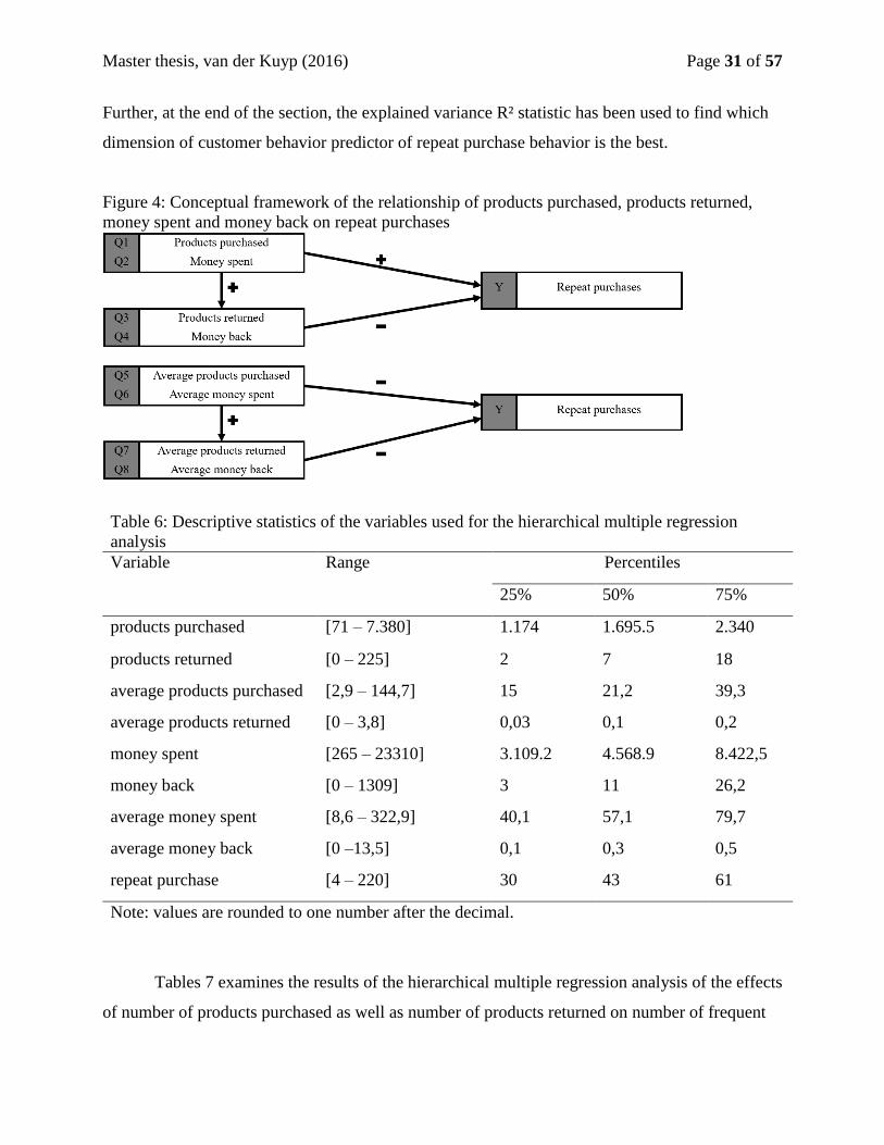
Following, the study conducts a hierarchical multiple regression analysis to test the
hypotheses. For the clarification of the 8 hypotheses, the same conceptual framework as Figure 1
has been presented below (see Figure 4). Further, Table 6 presents the descriptive statistics of the
key variables, which are used to interpret the regression coefficients b. The results have been
analyzed in the same order as the partial correlation analysis: starting with the hierarchical
multiple regression analysis of the effect of the number of products purchased (hypothesis 1) as
well as the effect of the number of products returned (hypothesis 3) on the number of frequent
repeat purchases, followed by the amount of money spend (hypothesis 2) and amount of money
back (hypothesis 4).
The hierarchical multiple regression analysis holds two levels. The first level analyzes the
regression coefficient b and the standardized regression coefficient β of the number of products
purchased on the number of frequent repeat purchases; and the regression coefficient b and the
standardized regression coefficient β number of products returned on the number of frequent
repeat purchases. Thereafter, the second level, tests the effects of both variables together using
the partial regression coefficient b and the standardized partial regression coefficient β. The
standardized regression coefficients β have been used to compare both effects which each other.
Master thesis, van der Kuyp (2016) Page 31 of 57
Further, at the end of the section, the explained variance R² statistic has been used to find which
dimension of customer behavior predictor of repeat purchase behavior is the best.
Figure 4: Conceptual framework of the relationship of products purchased, products returned,
money spent and money back on repeat purchases
Table 6: Descriptive statistics of the variables used for the hierarchical multiple regression
analysis
Variable Range Percentiles
25% 50% 75%
products purchased [71 – 7.380] 1.174 1.695.5 2.340
products returned [0 – 225] 2 7 18
average products purchased [2,9 – 144,7] 15 21,2 39,3
average products returned [0 – 3,8] 0,03 0,1 0,2
money spent [265 – 23310] 3.109.2 4.568.9 8.422,5
money back [0 – 1309] 3 11 26,2
average money spent [8,6 – 322,9] 40,1 57,1 79,7
average money back [0 –13,5] 0,1 0,3 0,5
repeat purchase [4 – 220] 30 43 61
Note: values are rounded to one number after the decimal.
Tables 7 examines the results of the hierarchical multiple regression analysis of the effects
of number of products purchased as well as number of products returned on number of frequent

Master thesis, van der Kuyp (2016) Page 32 of 57
repeat purchases. To start, the first two steps show that products purchased did significantly
predict repeat purchase, (b = 0,013, β = 0469, t = 34,27, p < 0,001), and that product returned
significantly predicts repeat purchases, (b = 0,163, β = 0,128, t = 8,35, p < 0,001). The variable of
products purchased ranges from 71 through 7.380 whereby 75% of the customers have purchased
between 71 and 2.340 products; and the variable products returned ranges from 0 through 225
whereby 75% of the customers have returned between 0 and 18 products (see Table 6). As
expected (based on previous correlation analysis), the standardized regression coefficient β of
products purchased is higher than the standardized regression coefficient β of products returned,
which mean that the effect of product return is the strongest predictor of repeat purchases.
Further, the explained variance R² indicates that the number of products purchased explain
around 22% of the variance in number of frequent repeat purchases whereas product returned
only explain 1,6% of the variance in number of frequent repeat purchases.
Testing both effects, the analysis shows that products returned did not significantly
predict repeat purchases, (b = -0,00, β = -0,002, t = -0,17, ns); however, products purchases
significantly predict repeat purchases, (b = 0,013, β = 0,470, t = 32,97, p < 0,001). Hypothesis 1,
which assumes that customers who purchase a higher number of products have a higher number
of frequent repeat purchases, is therefore confirmed. Further, the study rejects hypothesis 3 since
there is no significant differences in number of frequent repeat purchases between customers who
return more and less number of products.
Table 7: Hierarchical multiple regression analysis of products purchased and products returned
on repeat purchases
Variable b SE t P β R²
Step 1
Products purchased 0,013 0,000 34,27 < 0,001 0,469 0,220
Constant 25,020 0,771 32,43
Step 2
Products returned 0,163 0,019 8,35 < 0,001 0,128 0,016
Constant 46,217 0,483 95,65
Step 3
Products purchased 0,013 0,000 32,97 < 0,001 0,470 0,220
Products returned -0,003 0,018 -0,17 n.s. -0.002
Constant 25.030 0.773 32.36

Master thesis, van der Kuyp (2016) Page 33 of 57
Following, the study conducted a hierarchical multiple regression analysis to see if the
amount of money spent and the amount of money back (due to product return) predicted number
of frequent repeat purchases. Table 8 shows that money spent significantly predicted repeat
purchases, (b = 0,004, β = 0,456, t = 33,03, p < 0,001) and that money back significantly
predicted repeat purchases, (b = 0,096, β = 0,140, t = 9,11, p < 0,001). To interpreted the
regression coefficients, the variable money spent ranges from 265 through 23.310 whereas 75%
of the customers spends between 265 and 8.422 dollars; and the variable money back ranges from
0 through 1.309 whereas 75% of the customers get between 0 and 26 dollars back due to product
return. Considering the range of the variable money back, the regression coefficient b weakly
predicts the number of frequent repeat purchases. Further, the standardized regression coefficient
β for money spent is higher than the standardized regression coefficient β for money back. Thus
the amount of money customer spent predict the number of frequent repeat purchases better than
the amount of money customer get back (due to product return). Following, the amount of money
customers gets back (due to product return) explain only 2% of the variance in the number of
frequent repeat purchase; while the amount of money customers spends explain 20,7% of the
variance in the number of frequent repeat purchases.
Testing the effects of both variables, money spent significantly predicts repeat purchases,
(b = 0,004, β = 0,445, t = 31,69, p < 0,001) and money back significantly predicts repeat
purchases, (b = 0,034, β = 0,050, t = 3,58, p < 0,001). The study confirms hypothesis 2 since the
analysis show that customer who spent more amount of money have a higher number of frequent
repeat purchases. Noteworthy, is that the effect of money back on repeat purchases has almost
vanished when including the effect of money spent while the effect of money spent on repeat
purchases remains the same. This indicates that, taken into account the amount of money
customers spent, there are almost no differences in number of frequent repeat purchases, between
customers who get more amount of money back (due to product return) and customers who get
less amount of money back. The study rejects hypothesis 4, which assumes that customer who
get back more money (due to product return) have a lower number of repeat purchases.
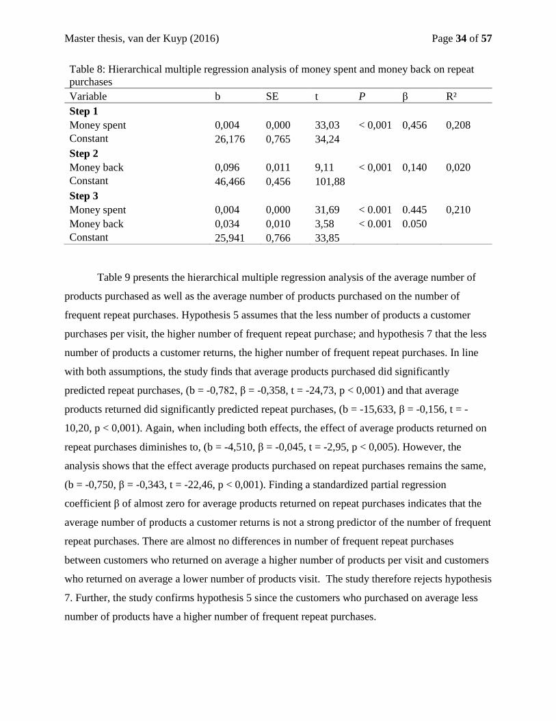
Master thesis, van der Kuyp (2016) Page 34 of 57
Table 9 presents the hierarchical multiple regression analysis of the average number of
products purchased as well as the average number of products purchased on the number of
frequent repeat purchases. Hypothesis 5 assumes that the less number of products a customer
purchases per visit, the higher number of frequent repeat purchase; and hypothesis 7 that the less
number of products a customer returns, the higher number of frequent repeat purchases. In line
with both assumptions, the study finds that average products purchased did significantly
predicted repeat purchases, (b = -0,782, β = -0,358, t = -24,73, p < 0,001) and that average
products returned did significantly predicted repeat purchases, (b = -15,633, β = -0,156, t = -
10,20, p < 0,001). Again, when including both effects, the effect of average products returned on
repeat purchases diminishes to, (b = -4,510, β = -0,045, t = -2,95, p < 0,005). However, the
analysis shows that the effect average products purchased on repeat purchases remains the same,
(b = -0,750, β = -0,343, t = -22,46, p < 0,001). Finding a standardized partial regression
coefficient β of almost zero for average products returned on repeat purchases indicates that the
average number of products a customer returns is not a strong predictor of the number of frequent
repeat purchases. There are almost no differences in number of frequent repeat purchases
between customers who returned on average a higher number of products per visit and customers
who returned on average a lower number of products visit. The study therefore rejects hypothesis
7. Further, the study confirms hypothesis 5 since the customers who purchased on average less
number of products have a higher number of frequent repeat purchases.
Table 8: Hierarchical multiple regression analysis of money spent and money back on repeat
purchases
Variable b SE t P β R²
Step 1
Money spent 0,004 0,000 33,03 < 0,001 0,456 0,208
Constant 26,176 0,765 34,24
Step 2
Money back 0,096 0,011 9,11 < 0,001 0,140 0,020
Constant 46,466 0,456 101,88
Step 3
Money spent 0,004 0,000 31,69 < 0.001 0.445 0,210
Money back 0,034 0,010 3,58 < 0.001 0.050
Constant 25,941 0,766 33,85

Master thesis, van der Kuyp (2016) Page 35 of 57
Table 9: Hierarchical multiple regression analysis of average products purchased and average
products returned on repeat purchases
Variable b SE t P β R²
Step 1
Average products purchased -0,782 0,032 -24,73 0 -0,358 0,128
Constant 66,853 0,832 80,37 0
Step 2
Average products returned -15,633 1,532 -10,20 0 -0,156 0,024
Constant 51,315 0,484 106,09 0
Step 3
Average products purchased -0,750 0,033 -22,46 0 -0,343 0,130
Average products returned -4,510 1,530 -2,95 0,003 -0,045
Constant 66,918 0,831 80,49 0
At last, the study conducted a hierarchical multiple regression analysis of the average
money spent as well as the average money revered on repeat purchases. Directly going to Step 3,
the analysis shows that average money spent significantly predicted repeat purchases (b = -0,273,
β = -0,346, t = -23,38, p < 0,001) and average money back significantly predicted repeat
purchases (b = -0,035, β = -0,035, t= -2,38 p < 0,05). Again, average money back has a
standardized partial regression coefficient of almost zero which indicates that the average amount
of money a customer gets back doesn’t predict the number of frequent repeat purchases. Based on
the results, the study confirms hypothesis 6 and rejects hypothesis 8.
Table 9: Hierarchical multiple regression analysis of average money spent and average money
back on repeat purchases
Variable b SE t P β R²
Step 1
Average money spent -0,279 0,011 -24,35 0 -0,353 0.125
Constant 66,277 0,822 80,68 0
Step 2
Average money back -5,980 0,879 -6,80 0 -0.105 0,011
Constant 50,098 0,464 108,00 0
Step 3
Average money spent -0,273 0,012 -23,38 0 -0,346 0,126
Average money back -2,010 0,844 -2,38 0.017 -0,035
Constant 66,459 0,825 80,6 0
Master thesis, van der Kuyp (2016) Page 36 of 57
To conclude, the results show that the number of products purchased and the amount of
money spent are the strongest predictors of future repeat purchases. The number of products that
customers purchase at a brick-and-mortar grocery retailing during this given period of time
explains around 22% of the variance in the number of frequent repeat purchases whereas the
amount of money spent explains around 21%. Further, the study finds that the average products
customers purchased and the average money customers spent also significantly predicted repeat
purchases. It confirms that customers who purchase on average less number of products visit as
well and spend on average less amount of money per visit, have a higher number of frequent
repeat purchases. The average number of products purchased has an explained variance of R²
=12,8% and the average amount of money spent an explained variance of R² = 12,5%.
Moreover, the analyses show that the number of products customers return explain only
1.6% of the variance in the number of frequent repeat purchases and the amount of money
customers get back (due to product return) explains only 2%. The same results hold for the
average of both variables whereby the average products returned has an explained variance of R²
=2,4% and the average money spent an explained variance of R² = 1,1%. At last, testing both the
effects of past purchase behavior and product return behavior, the study finds that the number of
products returned and the amount of money back (due to product return) did not predict the
number of repeat purchases. The analysis shows that differences in number of repeat purchases
are caused by the number of products customers purchased and the amount of money customers
spent; and not caused by the number of products customers returned and the amount of money
customers got back (due to products return).
Master thesis, van der Kuyp (2016) Page 37 of 57
VI. Discussion
Discussing the validity of the research design several remarks can be made. To start, the
Acquire Shopper Value dataset was originally designed to predict the effectiveness of coupon
promotions on repeat purchases of the promoted product. As stated “Part of the challenge of this
competition is learning the taxonomy of items in a data-driven way” (Acquired Valued Shopper
Challenge, 2014). This study focusses primarily on predicting repeat purchases at brick-and-
mortar grocery retailing. To protect customer and sales information the data is anonymized.
Based on the description of Kaggle, it is known that the selected brick-and-mortar grocery retailer
is located the United States since the transactions contain dollar values. Further we known that
the transactions contain information on customers that were selected for a coupon promotion and
redeemed this coupon.
Concerning the selection, it raises multiple questions on the external validity of the
results. Firstly, it could be that the results are biased towards a certain type of customers since all
customers were selected for a coupon promotion. For instance, when the grocery retailer selected
only loyal customers for the coupon promotion who visited the store more frequently than the
regular customers, the findings can only be generalize to this certain group of customers.
Secondly, the same line of reasoning could apply to the customer who did redeem the
coupon and customer who did not redeem the coupon. The study only shows the transactions of
the customers who redeemed the coupon. Yet, customers who redeem the coupon and customers
who did not redeem the coupon differ in purchase behavior the results can only be generalized
toward the former group.
Thirdly, it remains unknown whether the customer have a contract with the grocer
retailer. The grocery retailer collected transactional data on 32.640 customers from March 2 2012
through July 23 2013. Given the large amount of data, it is most likely that the grocery retailer
uses personalized customer cards which trace all the transaction information each visit (e.g. by
scanning their customer card during each visit). It could be that the customers pay a certain
amount of membership fee and that the If so, the external validity of the study only apply to a
contractual setting of brick-and-mortar grocery retailer.
Validating the internal validity, the study finds multiple systematic measurement errors in
the data. To start, the study finds inconsistencies in the transactions; that contain the return of a
product. 0,76% off all transactions recorded that a customer got money back while purchasing
Master thesis, van der Kuyp (2016) Page 38 of 57
one or more products. Given it is not possible to purchase a product and get money for
purchasing this product, the number of products purchased, of these transactions, have been
recoded to the number of products returned. However, the study isn’t completely certain whether
the recoding of products purchased to products returned is correct. The transactions could also be
recoded the other way around; recoding money back to money spend. The study assumes that
recoding the number of products has been a valid measurement of the number of products
returned.
Further, 0.34% of all transactions miss information on the number of products purchased,
the number of products returned, the amount of money spent and the amount of money back (due
to product return). Since the noise occurred across different customers it is assumed that results
are the same with no missing information. Kaggle has written the following note in response to
quality concerns of the data: “There are almost always thorny quality and consistency issues with
real world data, which could include label noise and a noisy ground truth. Also, in some cases we
choose not to try to correct for the noise or inconsistencies (or pretend they didn't exist by
dropping the corresponding rows), and instead provide the data in its raw form. This gives
competition participants the greatest flexibility determining how to handle inconsistencies present
in the data and prevents us from introducing additional noise in the process” (A Note On Quality,
2013).
Lastly, between March 2, 2012 through March 30, 2013 around 1.000 customers visit the
grocery retailer each day. The study finds that from March 30 2013 the data stops tracing all the
transactions. Kaggle didn’t provide any explanation for this and therefore the study removed all
transactions that occurred after March 30 2013. Yet, it could be possible that remaining data also
misses some transactions.
In this study the relationship between past purchase behavior as well as product return
behavior and repeat purchases behavior have been studied. We expect a positive relationship
between past purchase behavior and repeat purchase behavior; and a negative relationship
between product return behavior and repeat purchases behavior. To explain this positive
relationship, the study expects that customers who purchased more number of products and spent
more amount of money are the customers that visited the grocery retailing more frequently.
Following, customers who visited the store more frequently have a stronger relationship with the
grocery retailer and are therefore more likely to continue their purchase habits in the future. To

Master thesis, van der Kuyp (2016) Page 39 of 57
The study expects a negative relationship between product return behavior and repeat purchase
behavior because customers who returned more products are more likely to be disgusted and
therefore drop-out. The expectancy-disconfirmation model, expects that returning a product leads
to a negative affect about the grocery retailing because customers’ expectations about the product
are not met. Customers who return more products have more negative experience and are
therefore more likely to be disgusted with the grocery retailer.
Results confirm the positive relationship between past purchase behavior and repeat
purchase behavior. The number of products purchased and amount of money spent form the
strongest predictor of repeat purchases. Amount of money spent explain around 21% and number
of product purchased 22% of the variance in the number of frequent. However, the negative
relationship between product return behavior and repeat purchase behavior has not been found.
The analysis shows that differences in number of repeat purchases are caused by the number of
products customers purchased and the amount of money customers spent; and not caused by the
number of products customers returned and the amount of money customers got back (due to
products return). The relationship between product return behavior and repeat purchase behavior
has therefore been found spurious. Figure 5, examines the adjusted conceptual framework on the
relationship between past purchase behavior, product return behavior and repeat purchase
behavior.
Figure 5: Adjusted conceptual framework on products purchased, products returned, money spent
and money back.
Master thesis, van der Kuyp (2016) Page 40 of 57
Following, results show that the BG/NBD model did not perform well enough on this
particular data. The BG/NBD model assumes that customers purchase at a steady rate. However,
the used dataset contains a lot of customers that visited the grocery retailer almost every day. The
number of frequent visits on a short interval makes it difficult for the model to predict the future
purchases. As our analysis show, the predictions of the BG/NBD model were almost identical to
the frequency of buying (number of frequent visits). It is expected that the number of frequent visit
on a short interval have violated certain assumption of the model on the purchase behavior of
customers.
Some additional analysis has been done on the model to see the impact of this particular
data. Together with some fellow students from econometrics and mathematics we have used the
transaction data on the full timespan from March 02, 2012 through July 23, 2013 to validate the
model. Unfortunately, we have not been able empirically validity the model. To start, numerical
errors have been found for the same customers with extreme number of frequent visits on a short
interval. When estimating the parameters of the dropout rate and the purchase rate, customers with
more than 380 caused an error in the calculations of the maximum likelihood function. We have
tried to solve the errors in multiple ways like removing the customer with high number of purchases
or including customers with zero purchases. The only appropriate solution that we found was to
shorten the time period; and create a calibration period of 28 weeks which has been used for this
study. The additional analysis further confirms that the assumptions of the purchase behavior of
the BG/NBD have been violate due to the big group of customers with extreme number of visits
on a short interval.
The study recommends future studies to focus on using probabilistic customer base
analysis on brick-and-mortar grocery retailing. The study shows that repeat purchases at brick-and-
mortar grocery retailing are difficult to predict since this setting is characterized with firs
unobserved drop-out behavior, and second high customer heterogeneity in the frequency of visits.
Therefore, academics should apply different techniques predicting.
Master thesis, van der Kuyp (2016) Page 41 of 57
VII. Conclusion
This study proposes to answer the following question: Which dimensions of customer
behavior in a brick-and-mortar retailing setting predict the repeat purchases the best? It uses
transaction data on 4.017 customers of one brick-and-mortar grocery retailer made during the
period of March 2, 2012 through March 30, 2013. The data has been aggregated from transaction
level data to customer level data to form 8 different variables of customer behavior: the number
of products purchased, the average number of products purchased per visit, the amount of money
spent, the average amount of money spent, the number of products returned, the average number
of products purchased per visit, the amount of money back, and the average amount of money
back per visit. In addition, it uses the dependent variables predicted repeat purchases and repeat
purchases. The former has been calculated using the BG/NBD model which uses information on
the number of repeat purchases and the date of the last purchase during the first 28 weeks of the
time period to make a prediction of the number of frequent repeat purchases in the last 28 weeks.
The latter contains the actual repeat purchases of the customers made during the last 28 weeks of
the time period.
Results show that the BG/NBD model underperforms in comparison to a simple heuristic
model, which only uses the number of repeat purchases during the first 28 weeks of the time
period, to predict the repeat purchases. Therefore, the study uses the actual repeat purchases the
customers made during the last 28 weeks of the time period. The actual repeat purchases have
been used to test the relationship between past purchase behavior as well as product return
behavior and repeat purchase behavior.
Hypothesis 1 and 2 assume that customer who have purchased more number of products
and spent amount more money during the first 28 weeks will have a higher number of frequent
repeat purchases during the last 28 weeks. This is because customers that purchase more products
and spend more money during the first 28 weeks are the ones that visit the store more frequent.
Further, customer who visit the grocery retailer more often have a stronger relationship and are
more likely to continue their purchase habits during the last 28 weeks. Results confirm
hypothesis 1 and 2 and show that a higher number of products purchases and money spent results
in a higher number of frequent repeat purchases.
Furthermore, the study confirms hypothesis 5 and 6 which assume that customers who
purchase on average less number of products per visit and spend on average less amount on

Master thesis, van der Kuyp (2016) Page 42 of 57
money per visit have a higher number of frequent repeat purchases. This is because customers
who purchase less number of products per visit and spend less amount of money per visit are the
ones who have spread their groceries shopping’s across multiple visit. Again, the visit the store
more frequently, have a stronger relationship with the grocery retailer and continue their purchase
habits in the future.
At last, the study analyzes if customers who returns more number of products and get
back more amount of money (due to product return) have a lower number of frequent repeat
purchases. The expectancy-disconfirmation assume customers who return more number of
products as well as get back more amount of money (due to product return) are more likely to
have a negative experience with the grocery retailer which lead to customer disgust and less
future purchases. The analyses show that differences in number of repeat purchases are a caused
by the number of products a customer purchases and amount of money he spends; and not caused
by the number of products he returns and the amount of money het gets back (due to products
return). It confirms previous studies which show that customers dissatisfaction doesn’t necessary
lead to switching behavior. The study confirms the null-hypotheses 3, 4, 7 and 8 and rejects the
alternative hypotheses.
Overall, the number of products purchased forms the strongest predictors of number of
frequent repeat purchases followed by the amount of money spent. The number of products
purchased during explains 22% of variance in repeat purchases and he amount of money spent
explains 21 % of the variance in repeat purchases. Further the predictions of average products
purchased and average money spent both explain 12.8% and 12.5% of the variance in number of
frequent repeat purchases.
To explain the effect of “product return behavior” on repeat purchases behavior, the study
uses psychological constructs like negative affect, dissatisfaction and disgust. However, the
explanation of this effect is limited since the study uses only transaction data to test this. The
absence of evidence on the relationship between product return behavior and repeat purchases
doesn’t exclude that customer who return more products have more negative experiences or are
more dissatisfied. The area of product return behavior at brick-and-mortar grocery retailing is not
well studied. To get more knowledge about its influences this study strongly encourages future
studies to do more analysis. Both qualitative analysis and quantitative analysis could be used to

Master thesis, van der Kuyp (2016) Page 43 of 57
discover the underlying psychological constructs and find patterns between past purchase
behaviors.
At last, last the study presents some limitations and recommendations on the BG/NBD
model. The data is characterized with extreme frequent visit on short intervals which makes it
difficult to predict repeat purchases. As mentioned, the BG/NBD model did not perform well
enough on this particular data. Additional analysis shows that the model and the maximum
likelihood estimation could not be estimated on customers with extreme number of frequent visits
on a short interval. Using the full time period of 56 weeks, the maximum likelihood estimation
couldn’t estimate its parameters.
Master thesis, van der Kuyp (2016) Page 44 of 57
VIII. Bibliography
A Note On Data Quality. (2013). Kaggle Web site. Retrieved from
https://www.kaggle.com/wiki/ANoteOnDataQuality
Acquired Valued Shoppers Challenge. (2014) Kaggle Web site. Retrieved from
https://www.kaggle.com/c/acquire-valued-shoppers-challenge/data
Alexander, M. W. (2012). Delight the customer: A predictive model for repeat purchase
behavior. Journal of Relationship Marketing, 11(2), 116-123.
Anderson, E. W., & Mittal, V. (2000). Strengthening the satisfaction-profit chain. Journal of
Service Research, 3(2), 107-120.
Arons, M. D. S., van den Driest, F., & Weed, K. (2014). The ultimate marketing machine.
Harvard Business Review, 92(7), 54-63.
Avery, J., Fournier, S., & Wittenbraker, J. (2014). Unlock the mysteries of your customer
relationships. Harvard Business Review, 92(7), 8.
Binning, J. F., & Barrett, G. V. (1989). Validity of personnel decisions: A conceptual analysis of
the inferential and evidential bases. Journal of Applied Psychology, 74(3), 478.
Cheng, C., & Chen, Y. (2009). Classifying the segmentation of customer value via RFM model
and RS theory. Expert Systems with Applications, 36(3), 4176-4184.
Cokal, Murat. (2005). Freeimages Web site. Retrieved from
http://nl.freeimages.com/photo/grocery-cart-1426928
Master thesis, van der Kuyp (2016) Page 45 of 57
Dick, A. S., & Basu, K. (1994). Customer loyalty: Toward an integrated conceptual framework.
Journal of the Academy of Marketing Science, 22(2), 99-113.
Dwyer, F. R., Schurr, P. H., & Oh, S. (1987). Developing buyer-seller relationships. The Journal
of Marketing, , 11-27.
Fader, P. S., & Hardie, B. G. (2001). Forecasting repeat sales at CDNOW: A case study.
Interfaces, 31(3_supplement), S94-S107.
Fader, P. S., Hardie, B. G., & Lee, K. L. (2005). “Counting your customers” the easy way: An
alternative to the pareto/NBD model. Marketing Science, 24(2), 275-284.
Gupta, S., Hanssens, D., Hardie, B., Kahn, W., Kumar, V., Lin, N., . . . Sriram, S. (2006).
Modeling customer lifetime value. Journal of Service Research, 9(2), 139-155.
Johnson, B. (2016). Marketing in 2016: Focus on Relationships. PCMag.
Keaveney, S. M. (1995). Customer switching behavior in service industries: An exploratory
study. The Journal of Marketing, , 71-82.
Oliver, R. L. (1980). A cognitive model of the antecedents and consequences of satisfaction
decisions. Journal of Marketing Research, , 460-469.
Marketing Science Institute. (2013). Research Priorities 2014-2016. Retrieved December 11,
2015, from http://www.msi.org/uploads/files/MSI_RP14-16.pdf
Petrison, L. A., Blattberg, R. C., & Wang, P. (1997). Database marketing: Past, present, and
future. Journal of Interactive Marketing, 11(4), 109-125.
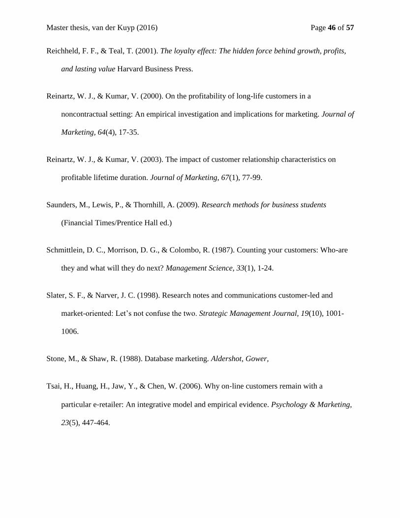
Master thesis, van der Kuyp (2016) Page 46 of 57
Reichheld, F. F., & Teal, T. (2001). The loyalty effect: The hidden force behind growth, profits,
and lasting value Harvard Business Press.
Reinartz, W. J., & Kumar, V. (2000). On the profitability of long-life customers in a
noncontractual setting: An empirical investigation and implications for marketing. Journal of
Marketing, 64(4), 17-35.
Reinartz, W. J., & Kumar, V. (2003). The impact of customer relationship characteristics on
profitable lifetime duration. Journal of Marketing, 67(1), 77-99.
Saunders, M., Lewis, P., & Thornhill, A. (2009). Research methods for business students
(Financial Times/Prentice Hall ed.)
Schmittlein, D. C., Morrison, D. G., & Colombo, R. (1987). Counting your customers: Who-are
they and what will they do next? Management Science, 33(1), 1-24.
Slater, S. F., & Narver, J. C. (1998). Research notes and communications customer-led and
market-oriented: Let’s not confuse the two. Strategic Management Journal, 19(10), 1001-
1006.
Stone, M., & Shaw, R. (1988). Database marketing. Aldershot, Gower,
Tsai, H., Huang, H., Jaw, Y., & Chen, W. (2006). Why on‐line customers remain with a
particular e‐retailer: An integrative model and empirical evidence. Psychology & Marketing,
23(5), 447-464.
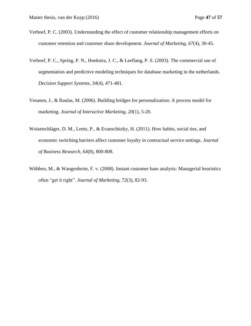
Master thesis, van der Kuyp (2016) Page 47 of 57
Verhoef, P. C. (2003). Understanding the effect of customer relationship management efforts on
customer retention and customer share development. Journal of Marketing, 67(4), 30-45.
Verhoef, P. C., Spring, P. N., Hoekstra, J. C., & Leeflang, P. S. (2003). The commercial use of
segmentation and predictive modeling techniques for database marketing in the netherlands.
Decision Support Systems, 34(4), 471-481.
Vesanen, J., & Raulas, M. (2006). Building bridges for personalization: A process model for
marketing. Journal of Interactive Marketing, 20(1), 5-20.
Woisetschläger, D. M., Lentz, P., & Evanschitzky, H. (2011). How habits, social ties, and
economic switching barriers affect customer loyalty in contractual service settings. Journal
of Business Research, 64(8), 800-808.
Wübben, M., & Wangenheim, F. v. (2008). Instant customer base analysis: Managerial heuristics
often “get it right”. Journal of Marketing, 72(3), 82-93.
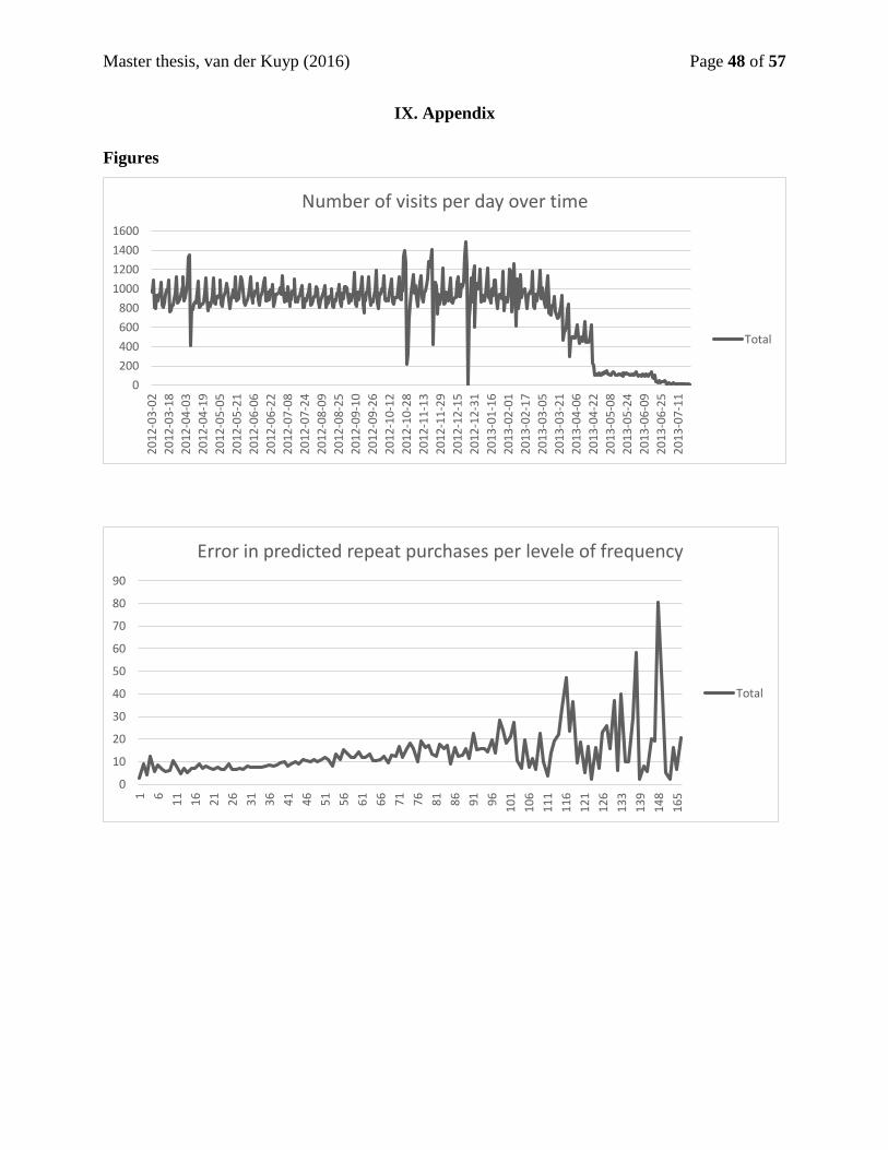
Master thesis, van der Kuyp (2016) Page 48 of 57
IX. Appendix
Figures
0
200
400
600
800
1000
1200
1400
1600
20
12
-03
-02
20
12
-03
-18
20
12
-04
-03
20
12
-04
-19
20
12
-05
-05
20
12
-05
-21
20
12
-06
-06
20
12
-06
-22
20
12
-07
-08
20
12
-07
-24
20
12
-08
-09
20
12
-08
-25
20
12
-09
-10
20
12
-09
-26
20
12
-10
-12
20
12
-10
-28
20
12
-11
-13
20
12
-11
-29
20
12
-12
-15
20
12
-12
-31
20
13
-01
-16
20
13
-02
-01
20
13
-02
-17
20
13
-03
-05
20
13
-03
-21
20
13
-04
-06
20
13
-04
-22
20
13
-05
-08
20
13
-05
-24
20
13
-06
-09
20
13
-06
-25
20
13
-07
-11
Number of visits per day over time
Total
0
10
20
30
40
50
60
70
80
90
1 6
11
16
21
26
31
36
41
46
51
56
61
66
71
76
81
86
91
96
10
1
10
6
11
1
11
6
12
1
12
6
13
3
13
9
14
8
16
5
Error in predicted repeat purchases per levele of frequency
Total

Master thesis, van der Kuyp (2016) Page 49 of 57
Tables
Percentages of products purchased per price
_Price Percentage Cumulative
0 – 0,50 1.20 1.20
0,50 – 1 9.38 10.58
1 – 2 27.24 37.82
2 – 3 28.01 65.83
3 – 4 16.86 82.69
4 – 5 7.63 90.32
5 – 10 7.94 98.26
10 – 20 1.46 99.72
20 – 50 0.27 99.99
50 – 100 0.01 100.00
Percentages of products returned per price
Price Percentage Cumulative
0 – 0,50 13.58 13.58
0,50 – 1 62.81 76.39
1 – 2 12.71 89.10
2 – 3 3.70 92.80
3 – 4 2.49 95.29
4 – 5 3.19 98.49
5 – 10 1.26 99.75
10 – 20 0.15 99.90
20 – 80 0.10 100.00
Percentages of products purchased per price
Price Percentage Cumulative
0 – 5 6.48 6.48
5 – 10 8.55 15.03
10 – 20 14.90 29.93
20 – 30 11.61 41.54
30 – 40 9.15 50.69
40 – 50 7.55 58.24
50 – 100 23.71 81.95
100 – 150 10.78 92.73
150 – 200 4.49 97.21
200 – 250 1.75 98.96
250 – 300 0.63 99.59
300 – 400 0.34 99.93
400 – 500 0.06 99.99
< 500 0.01 100.00
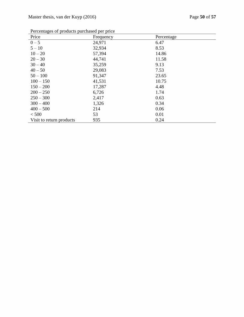
Master thesis, van der Kuyp (2016) Page 50 of 57
Percentages of products purchased per price
Price Frequency Percentage
0 – 5 24,971 6.47
5 – 10 32,934 8.53
10 – 20 57,394 14.86
20 – 30 44,741 11.58
30 – 40 35,259 9.13
40 – 50 29,083 7.53
50 – 100 91,347 23.65
100 – 150 41,531 10.75
150 – 200 17,287 4.48
200 – 250 6,726 1.74
250 – 300 2,417 0.63
300 – 400 1,326 0.34
400 – 500 214 0.06
< 500 53 0.01
Visit to return products 935 0.24
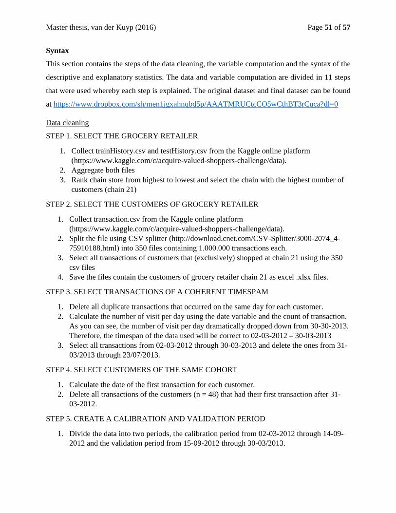
Master thesis, van der Kuyp (2016) Page 51 of 57
Syntax
This section contains the steps of the data cleaning, the variable computation and the syntax of the
descriptive and explanatory statistics. The data and variable computation are divided in 11 steps
that were used whereby each step is explained. The original dataset and final dataset can be found
at https://www.dropbox.com/sh/men1jgxahnqbd5p/AAATMRUCtcCO5wCthBT3rCuca?dl=0
Data cleaning
STEP 1. SELECT THE GROCERY RETAILER
1. Collect trainHistory.csv and testHistory.csv from the Kaggle online platform
(https://www.kaggle.com/c/acquire-valued-shoppers-challenge/data).
2. Aggregate both files
3. Rank chain store from highest to lowest and select the chain with the highest number of
customers (chain 21)
STEP 2. SELECT THE CUSTOMERS OF GROCERY RETAILER
1. Collect transaction.csv from the Kaggle online platform
(https://www.kaggle.com/c/acquire-valued-shoppers-challenge/data).
2. Split the file using CSV splitter (http://download.cnet.com/CSV-Splitter/3000-2074_4-
75910188.html) into 350 files containing 1.000.000 transactions each.
3. Select all transactions of customers that (exclusively) shopped at chain 21 using the 350
csv files
4. Save the files contain the customers of grocery retailer chain 21 as excel .xlsx files.
STEP 3. SELECT TRANSACTIONS OF A COHERENT TIMESPAM
1. Delete all duplicate transactions that occurred on the same day for each customer.
2. Calculate the number of visit per day using the date variable and the count of transaction.
As you can see, the number of visit per day dramatically dropped down from 30-30-2013.
Therefore, the timespan of the data used will be correct to 02-03-2012 – 30-03-2013
3. Select all transactions from 02-03-2012 through 30-03-2013 and delete the ones from 31-
03/2013 through 23/07/2013.
STEP 4. SELECT CUSTOMERS OF THE SAME COHORT
1. Calculate the date of the first transaction for each customer.
2. Delete all transactions of the customers (n = 48) that had their first transaction after 31-
03-2012.
STEP 5. CREATE A CALIBRATION AND VALIDATION PERIOD
1. Divide the data into two periods, the calibration period from 02-03-2012 through 14-09-
2012 and the validation period from 15-09-2012 through 30-03/2013.

Master thesis, van der Kuyp (2016) Page 52 of 57
Variable computation
In the screenshot the variables of the transaction.xlsx files are presented. The values in column J
respond to the number of products purchased or returned and the values in column K to the
amount of money spent or regained for this product.
STEP 0: RECALCULATE PURCHASEQUANTITY AND PURCHASEAMOUNT
Two types of inconsistencies (see the highlighted cells) are adjusted: 1) transactions that contains
product return and money spent 2) transactions that contain product purchased and money back.
1. Recalculate purchasequantity by inserting the formula = IF(AND(K2<0; M2>0); J2*-1;
J2) in cell L2
2. Recalculate purchaseamount by inserting the formula = =IF(AND(J2<0; K2>0);K2* -1;
K2) in cell M2
3. Drag L2 and M2 through the last row
4. Copy column L and M
5. Paste values in J and M
6. Delete column Land M
STEP 1. CALCULATE THE PURCHASEQUANTITY AND PURCHASEAMOUNT
POSITIVE AND NEGATIVE
1. Calculate purchasequantity positive by inserting the formula =IF(K2>-0.001; J2;0) in cell
L2.
2. Calculate purchasequantity negative by inserting the formula =IF(K2>-0.001; J2;0) in cell
M2.
3. Drag L2 and M2 through the last row.
STEP 2. CALCULATE PURCHASEAMOUNT POSITIVE AND NEGATIVE

Master thesis, van der Kuyp (2016) Page 53 of 57
1. Calculate purchaseamount positive by inserting the formula =IF(K2>-0.001; J2;0) in cell
N2
2. Calculate purchaseamount negative by inserting the formula =IF(K2>-0.001; J2;0) in cell
O2
3. Drag N2 and O2 through the last row
STEP 3. ADD UP THE NUMBERS OF PRODUCTS PURCHASED AND RETURNED PER
VISIT
1. Add up the numbers of products purchased by inserting the formula =IF(AND(A1=A2;
G1=G2); L2+P1; L2) in cell P2
2. Add up the numbers of products returned by inserting the formula =IF(AND(A1=A2;
G1=G2); M2+Q1; M2) in cell Q2
3. Drag P2 and Q2 to the last row
STEP 4: ADD UP THE AMOUNT OF MONEY SPENT AND REGAINED PER VISIT
1. Add up the amount of money spent per visit by inserting the formula =IF(AND(A1=A2;
G1=G2); N2+R1; N2) in cell R2
2. Add up the amount of money back per visit by inserting the formula =IF(AND(A1=A2;
G1=G2); O2+S1; O2) in cell S2
3. Drag R2 and S2 to the last row
STEP 5: REMOVE ALL DUPLICATE TRANSACTIONS OF EACH VISIT
1. Code all duplicate transaction with a 0 by inserting the formula =IF(AND(A2=A3;
G2=G3); 0; 1) in cell T2
2. Drag T2 to the last row
3. Select and cope all cells
4. Use “paste values” in cell A1
5. Select all cells
6. Sort the cells on the duplicate variables from lowest to highest value
7. Remove all transactions coded with a 0
STEP 6: CALCUATE IF THE TRANSACTION IS THE FIRST PURCHASE, CALIBRATION
PERIOD OR VALIDATION PERIOD
1. Calculate the value of each date by inserting the formula =DATEVALUE(G2) in cell U2.
2. Calculate the period by inserting the formula
=IF(A2<>A1;"first";IF(U2<=41166;"calib";"valid")) in cell V2. (41166 is date value of
14 September 2012).
3. Drag V2 and W2 through the last row.
STEP 7: CALCULATE THE DATE OF FIRST PURCHASE AND LAST PURCHASE
1. Calculate the date of the first purchase by inserting the formula =IF(AND(A2<>A1;
U2<=41166); U2;0) in cell X2.

Master thesis, van der Kuyp (2016) Page 54 of 57
2. Calculate the date of the last purchase by inserting the formula =IF(U2<=41166;
IF(OR(A2<>A3; U3>41166); U2;0);0) in the Y2.
STEP 8: COMPUTE THE VARIABLE FREQUENCY OF BUYING AND REPEAT
PURCHASES
1. Highlight all cells and create a Pivot Table in the new sheet.
2. Rename the sheet as Pivot Table 1.
3. Use ID (column A) as the row field, Period (column V) as the column field, and ID using
the count option as the data item.
4. Name column B “frequency” and column D “repeat purchases”
STEP 9. COMPUTE THE VARIABLE PRODCUTS PURCHASED AND PRODUCTS
RETURNED
1. Highlight all cells and create a Pivot Table in the new sheet.
2. Rename the sheet as Pivot Table 2.
3. Use ID (column A) as the row field, Period (column V) as the column field, and products
purchased (column P) and products returned (column Q) using the average and sum
option as the data item.
4. Name column B “average products purchased per visit” and column C “average products
returned per visit”
5. Name column D “Total products purchased” and column E “Total products returned”
STEP 10. COMPUTE THE VARIABLE MONEY SPENT AND MONEY BACK
1. Highlight all cells and create a Pivot Table in the new sheet.
2. Rename the sheet as Pivot Table 3.
3. Use ID (column A) as the row field, Period (column V) as the column field, and money
spent (column R) and money back (column S) using the average and sum option as the
data item.
4. Name column B “average money spent per visit” and column C “average money spent per
visit”
5. Name column D “Total money spent” and column E “Total money back”
STEP 11. COMPUTE THE VARIABLE PERIOD OF PURCHASE
1. Highlight all cells and create a Pivot Table in the new sheet.
2. Rename the sheet as Pivot Table 4.
3. Use ID (column A) as the row field and first purchase (column W), using the sum option,
as the data item.
4. Calculate the purchase period by inserting the formula =(DATE(2012;9;14)-B4)/7 in cell
C4.
5. Name column C “period of purchase”
STEP 12. COMPUTE THE VARIABLE RECENCY
1. Highlight all cells and create a Pivot Table in the new sheet.
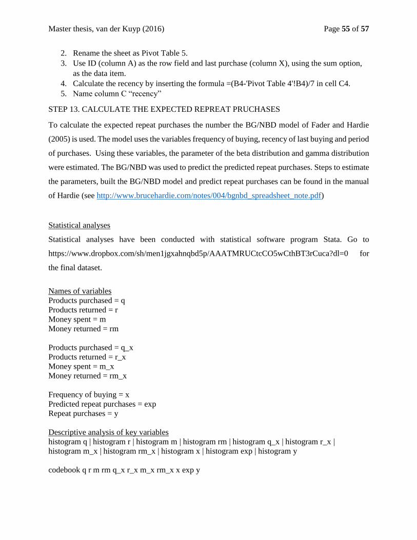
Master thesis, van der Kuyp (2016) Page 55 of 57
2. Rename the sheet as Pivot Table 5.
3. Use ID (column A) as the row field and last purchase (column X), using the sum option,
as the data item.
4. Calculate the recency by inserting the formula =(B4-'Pivot Table 4'!B4)/7 in cell C4.
5. Name column C “recency”
STEP 13. CALCULATE THE EXPECTED REPREAT PRUCHASES
To calculate the expected repeat purchases the number the BG/NBD model of Fader and Hardie
(2005) is used. The model uses the variables frequency of buying, recency of last buying and period
of purchases. Using these variables, the parameter of the beta distribution and gamma distribution
were estimated. The BG/NBD was used to predict the predicted repeat purchases. Steps to estimate
the parameters, built the BG/NBD model and predict repeat purchases can be found in the manual
of Hardie (see http://www.brucehardie.com/notes/004/bgnbd_spreadsheet_note.pdf)
Statistical analyses
Statistical analyses have been conducted with statistical software program Stata. Go to
https://www.dropbox.com/sh/men1jgxahnqbd5p/AAATMRUCtcCO5wCthBT3rCuca?dl=0 for
the final dataset.
Names of variables
Products purchased = q
Products returned = r
Money spent = m
Money returned = rm
Products purchased = q_x
Products returned = r_x
Money spent = m_x
Money returned = rm_x
Frequency of buying = x
Predicted repeat purchases = exp
Repeat purchases = y
Descriptive analysis of key variables
histogram q | histogram r | histogram m | histogram rm | histogram q_x | histogram r_x |
histogram m_x | histogram rm_x | histogram x | histogram exp | histogram y
codebook q r m rm q_x r_x m_x rm_x x exp y
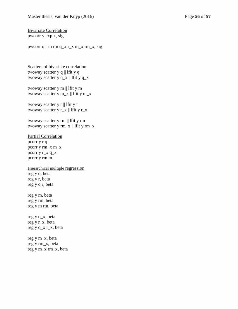
Master thesis, van der Kuyp (2016) Page 56 of 57
Bivariate Correlation
pwcorr y exp x, sig
pwcorr q r m rm q_x r_x m_x rm_x, sig
Scatters of bivariate correlation
twoway scatter y q || lfit y q
twoway scatter y q_x || lfit y q_x
twoway scatter y m || lfit y m
twoway scatter y m_x || lfit y m_x
twoway scatter y r || lfit y r
twoway scatter y r_x || lfit y r_x
twoway scatter y rm || lfit y rm
twoway scatter y rm_x || lfit y rm_x
Partial Correlation
pcorr y r q
pcorr y rm_x m_x
pcorr y r_x q_x
pcorr y rm m
Hierarchical multiple regression
reg y q, beta
reg y r, beta
reg y q r, beta
reg y m, beta
reg y rm, beta
reg y m rm, beta
reg y q_x, beta
reg y r_x, beta
reg y q_x r_x, beta
reg y m_x, beta
reg y rm_x, beta
reg y m_x rm_x, beta