predicting call arrivals in call centers · predicting call arrivals in call centers koen van den...

3

Predicting Call Arrivals in Call Centers

Koen van den Bergh

BMI-Paper

Supervisor: drs. A. Pot

Vrije Universiteit

Faculty of Sciences discipline Business Mathematics & Informatics

De Boelelaan 1081a 1081 HV Amsterdam

The Netherlands

August 2006

Executive Summary

Even though there is an enormous amount written about forecasting, the number of arti-cles about call center forecasting is not very impressive. The articles capture a reasonableamount of mathematical forecasting models, but the many undiscovered models can beapplied to enhance the accuracy of forecasting. Great-scale research will be needed tobroaden the knowledge about this subject.

In this paper a complete literature overview of different forecasting methods is provided,with a particular focus on the forecasting methods that are expounded and utilized forpredicting daily call frequencies in call centers.

After the explanation of these methods, two of them are tested using a real call centerdatabase. The results and all what enters into the forecast will be discussed in this paper.

In conclusion a comparison will be given of the differences and the advantages / disad-vantages of the different methods.

Preface

One of the graduate courses of my study Business Mathematics & Informatics is the courseBMI-paper. In this course one can chose a subject to gain more in-depth knowledge. Asthe name of my study indicates, it captures three components: economics, mathematics,and Informatics. In my paper all three components are included.

I have tried to setup a clear and complete overview regarding the existing mid-term callcenter call frequency forecasting techniques. If there are any notes or suggestions regardingthis paper, I sincerely like to hear from you.

I enjoyed working on this project. Although the subject discussed in this paper has notbeen treated during my study, by working on this paper I did get the opportunity to godeeply into this matter.

Besides the examination of the possible forecast methods, some of the forecast methodswere actually done. Most fascinating was to see that the discussed models transformed adatabase into good forecasts.

It is clear that the prediction of call center arrivals is still in its infancy and that there isa lot more to discover. Hereby I would like to stimulate other people that are interestedin this matter to further investigate the forecasting of call center arrivals, so that moreknowledge can be gained.

To conclude I would like to thank my supervisor Auke Pot for the effort and time spent. Ienjoyed our cooperation and he helped me in many aspects.

I sincerely hope that you will enjoy reading this paper as much as I enjoyed writing it.

With kind regards,

Koen van den Bergh

Contents

1 Introduction 3

2 Forecasting Models 52.1 ARIMA Model . . . . . . . . . . . . . . . . . . . . . . . . . . . . . . . . . 52.2 Dynamic Regression Models . . . . . . . . . . . . . . . . . . . . . . . . . . 72.3 Exponential Smoothing . . . . . . . . . . . . . . . . . . . . . . . . . . . . . 12

2.3.1 Single Exponential Smoothing . . . . . . . . . . . . . . . . . . . . . 122.3.2 Holt’s Linear Model . . . . . . . . . . . . . . . . . . . . . . . . . . 132.3.3 Holt-Winters’ Trend and Seasonality Model . . . . . . . . . . . . . 14

2.4 Regression Analysis . . . . . . . . . . . . . . . . . . . . . . . . . . . . . . . 15

3 Applying Techniques 193.1 Data . . . . . . . . . . . . . . . . . . . . . . . . . . . . . . . . . . . . . . . 193.2 Software . . . . . . . . . . . . . . . . . . . . . . . . . . . . . . . . . . . . . 213.3 Measurements of Forecasting Accuracy . . . . . . . . . . . . . . . . . . . . 233.4 Forecasting Results . . . . . . . . . . . . . . . . . . . . . . . . . . . . . . . 23

3.4.1 ARIMA Model Predictions . . . . . . . . . . . . . . . . . . . . . . . 253.4.2 Holt-Winters’ Trend and Seasonality Model Predictions . . . . . . . 273.4.3 Summary of Results . . . . . . . . . . . . . . . . . . . . . . . . . . 28

3.5 Suggestions for Improvement . . . . . . . . . . . . . . . . . . . . . . . . . . 29

4 Conclusions and Further Research 31

5 Appendix 355.1 ARIMA Functions R-code . . . . . . . . . . . . . . . . . . . . . . . . . . . 355.2 Holt-Winters Functions R-code . . . . . . . . . . . . . . . . . . . . . . . . 365.3 Error R-code . . . . . . . . . . . . . . . . . . . . . . . . . . . . . . . . . . 375.4 Charts of the Predictions . . . . . . . . . . . . . . . . . . . . . . . . . . . . 39

2 Predicting Arrivals in Call Centers

Chapter 1

Introduction

The main purpose of this paper is to provide a complete literature overview of differentforecasting methods, with a particular focus on the forecasting methods that are expoundedand utilized for predicting call frequencies in call centers. Before proceeding, a short ex-pound will be given of a call center.

A call center is a centralized office within a company that both answers incoming andmakes outgoing telephone calls to clients (telemarketing). An important task of call cen-ters is staffing. If too many staff members are scheduled at the same time, this will causelow efficiency and high costs. On the other hand, the benefit is that all incoming calls canbe dealt with, and thus there will be fewer discontented clients. The result of not schedul-ing enough call center workers will be low costs and highly efficient telephone clerks. Anegative outcome, however, may be that the number of incoming calls exceed the numberof available clerks. Many calls will remain unanswered, which shall cause dissatisfactionand eventually even loss of clients. The result of such a scenario will be a loss of sales andthus a loss of income.

The main issue is thus to find a balance. This means scheduling enough staff members sothat every call can be handled, except in very rare circumstances. This way, the opera-tional costs will be kept as low as possible and the clients are satisfied simultaneously. Inorder to compute the right number of staff members, a database of daily call volumes mustbe available. With the help of this database and a mathematical forecasting method it ispossible to forecast the daily expected calls. Self-evidently, the number of telephone clerksneeded, can be computed by means of these daily expected calls.

As one might understand commercial firms have great interest in forecasting the rightnumber of personnel, seeing the advantages of investing little money and still reachinghigh efficiency.

Even though there is an enormous amount written about forecasting, the number of articlesabout call center forecasting is not very impressive. In an assessment of future directions

3


for call center research, Gans, Koole, and Mandelbaum [8] even write that the practice oftime series forecasting at call centers is ”still in its infancy”.

A distinction can be made between the articles written about forecasting call frequen-cies. There are three periods of time that are subject to the forecasting. One can forecaston the long term, the mid term, and on the short term. Longer term forecasts such asyearly and monthly predictions, are used for budgeting and staff planning, planning op-erational changes, training, and scheduling vacations. Mid term forecasts, such as weeklyand daily forecasts, are needed for workforce staffing and scheduling. Short term forecasts,such as hourly, measure how well a call center is staffed for the current day. Tradition-ally, short term forecasts have been defined as making predictions for periods of less thanthree months. Medium forecasts span the three months to two year time frame and longterm forecasts deal with any period of time longer than two years. However, in call cen-ter applications, these time frames are often difficult to predict and may not be very useful.

The focus in this paper is forecasting daily call volumes. This means that several methodsused in previous papers on the topic of mid term forecasting will be expounded.

After the explanation of these methods, two of them will be tested using a real call centerdatabase. The results and all what enters into the forecast will be discussed in the chapterApplying Techniques.

In the last chapter the conclusions of this research will be given together with some direc-tions for further research.

Chapter 2

Forecasting Models

Previous scholarly texts have shown that there are several methods to be used for fore-casting time series. However, not all of the existing forecasting methods are applied toforecast call frequencies at call centers. In this section, an overview of the models used willbe presented. For each method, the model will be given together with the accompanyingliterature in which the models were used. In none of the articles about forecasts for callcenters the specific model applied was shown. Therefore, it is only possible to give a generalmodel. Subsequently, the following models are discussed:

• ARIMA Model

• Dynamic Regression Models

• Exponential Smoothing

• Regression Analysis

2.1 ARIMA Model

ARIMA is the abbreviation for AutoRegressive Integrated Moving Average. The ARIMAmodel is a widely used forecasting model invented by Box and Jenkins [5]. The basis of theARIMA model is the ARMA model, which consists of two sorts of terms: the autoregressiveterms (AR) and the moving average (MA) terms.

Autoregressive (AR) terms are lagged values of the dependent variable, and serve asindependent variables in the model. The General autoregressive model is given by

yt = α + φ1yt−1 + φ2yt−2 + . . . + φpyt−p + εt, t = p + 1, p + 2, . . . , p + n. (2.1)

Here φ1, . . . , φp and α are unknown parameters. The process εt is white noise with theproperty that E[εtyt−k] = 0 for all k ≥ 1. So the regressors yt−k are exogeneous with

5


k = 1, . . . , p. As the time series yt is observed for t = 1, . . . , n, the p-lagged explanatoryvariable is available only from time t = p+1 onwards. This model is called an autoregressivemodel of order p, also written as AR(p).

Moving Average (MA) terms are lagged values of the errors between past actualvalues and their predicted values who also serve as independent variables. A generalMoving average process is given by the next formula

yt = α + εt + θ1εt−1 + . . . + θqεt−q, (2.2)

where εt is white noise. Here α and θ1, . . . , θq are unknown parameters. This process is al-ways stationary, with mean µ = E[yt] = α, variance γ0 = σ2(1+

∑qj=1 θ2

j ), and covariances

γk = σ2(θk +∑q

j=k+1 θjθj−k) for k ≤ q and yk = 0 for k > q. This model is also known asa moving average model of order q, which can be written as MA(q).

Combining both models gives the autoregressive moving average model, also known asARMA(p, q)

yt = φ1yt−1 + φ2yt−2 + . . . + φpyt−p + εt + θ1εt−1 + . . . + θqεt−q. (2.3)

To denote this formula in a more concise way, lag operators are used. Applying lag operator(denoted L) once, the index is moved back one time unit and if this is applied k times, theindex is moved back k units.

Lyt = yt−1,

L2yt = yt−2,

...,

Lkyt = yt−k,

The lag operator is distributive over the addition operator, i.e.

L(εt + yt) = εt−1 + yt−1.

By using lag operators it is possible to rewrite the ARMA models using lag operators,which is done in equation (2.4).

AR(p) : (1− φ1L− φ2L2 − . . .− φpL

p)yt = εt,

MA(q) : yt = (1 + θ1L + θ2L2 + . . . + θqL

q)εt. (2.4)

With the lag polynomials

Forecasting Models 7

φ(L) = 1− φ1L− φ2L2 − . . .− φpL

p,θ(L) = 1 + θ1L + θ2L

2 + . . . + θqLq,

it is possible to rewrite an ARMA process in a more compact way:

AR : φ(L)yt = εt,

MA : yt = θ(L)εt,

ARMA : φ(L)yt = θ(L)εt. (2.5)

The I in ARIMA indicates integrated and refers to the practice of differencing, whichtransforms a time series by subtracting past values from itself. The ARIMA(p,d,q) isgiven by

φ(L)(1− L)dyt = α + θ(L)εt, (2.6)

where d is the indication of the amount of past values that is used to subtract itself. So farthe description of the ARIMA model. For a comprehensive expound of the ARIMA modelthe reader is pointed to the book of Heij et al [9].

Forecasting practitioners have long realized the potential of the ARIMA methodology formodeling time series data with strong seasonal patterns. In fact, most articles on fore-casting call volumes in call centers refer to the ARIMA model. Nijdam [14] illustrated theeffectiveness of ARIMA models for predicting monthly telephone traffic in the presence of apersistent seasonal pattern. In the most recent article, W. Xu [16], a Forecasting Specialistin the Forecasting/Modeling Group in Worldwide Customer Service Strategic Planning &Analysis at FedEx explained that ARIMA is one of the forecasting models used in SAS,their major forecasting software.

2.2 Dynamic Regression Models

The ARIMA model discussed in the previous section deals with single time series anddoes not allow the inclusion of other information in the models and forecasts. However,frequently other information may be used to aid in forecasting time series. Informationabout holidays, strikes, changes in the law, or other external variables may be of use inassisting the development of more accurate forecasts.

An example of this type of useful information is the influence of advertising campaigns.Often the effect such of information does not show up in the forecast variable (yt) immedi-ately, but is divided across several time periods. For instance, the effect of an advertisingcampaign persists for some time after the end of the campaign. In this case, monthly salesfigures (yt) may be modeled as a function of the advertising costs in each of the previous


few months, that is xt, xt−1, xt−2, . . .. So, the output series, yt is affected by the inputseries, xt. In fact, the input series xt influences the output series yt over several future timeperiods.

The general dynamic regression model is give by the next equation

yt = a + ν0xt + ν1xt−1 + ν2xt−2 + . . . + νkxt−k + nt. (2.7)

Here yt denotes the output time series and xt, xt−1, . . . , xt−k denotes the input time series.nt is an ARIMA process as described in the previous section. The values ν0, . . . , νk presentthe so-called impulse response weights (also transfer function weights). These coefficientsare measures of how yt is affected by xt−i. The general dynamic regression model equationcan be rewritten to make the formula shorter. This is done in the following way

yt = a + ν0xt + ν1xt−1 + ν2xt−2 + . . . + νkxt−k + nt,

= a + (ν0 + ν1L + ν2L2 + . . . + νkL

k)xt + nt,

= a + ν(L)xt + nt. (2.8)

In this shorthand notation ν(L) is called the transfer function since it describes how achange in the explanatory variable xt is transferred to yt. As can be seen, the lag operator,which was explained in the previous subsection, is also being applied here. Owing to this,the Equation (2.8) can be written in a more compact way.

The order of the transfer function is k, which is the longest lag in x that is used. Thisorder can sometimes be very large. For this reason, the dynamic regression model will bewritten in a more parsimonious form. This rewritten form is as follows

yt = a +ω(L)

δ(L)xt−l + nt, (2.9)

where

ω(L) = ω0 − ω1L− ω2L2 − . . .− ωsL

s,δ(L) = 1− δ1L− δ2L

2 − . . .− δrLr,

and r, s, and b constants.

In this model the two polynomials, ω(L) and δ(L), replace the polynomial ν(L), whichreduces the number of parameters to estimate, making more efficient use of the data andso producing more accurate forecasts. Note that the subscript for x is (t− l). This meansthat there is a delay of l periods before x begins to influence y. So xt−l influences yt first.When l > 0, x is often called a ”leading indicator” since xt is leading yt by l periods.


The reason why this rewritten form is more parsimonious is that the values of r and sare usually going to be much smaller than the value of k. This will be illustrated y thenext example. Suppose ω(L) = 1.2− 0.5L and δ(L) = 1− 0.8L. Then

ω(L)

δ(L)=

1.2− 0.5L

1− 0.8L,

= (1.2− 0.5L)(1− 0.8L)−1,

= (1.2− 0.5L)(1 + 0.8L + 0.82L2 + 0.83L3 + . . .),

= 1.2 + 0.46L + 0.368L2 + 0.294L3 + 0.236L4 + . . . ,

= ν(L). (2.10)

In this case, ν(L) would have had an immensely large order number k, while ω(L) andδ(L) would have had respectively an order of r = 1 and s = 1. Therefore, the restatedmodel is more parsimonious.

It is straightforward to extend the dynamic regression model to include several explanatoryvariables, such that solutions can be tractable. In case of an additive relation between theexplanatory variables the formula is given by Equation (2.11)

yt = a +m∑

i=1

Lliωi(L)

δi(L)xi,t + nt,

= a +m∑

i=1

ωi(L)

δi(L)xi,t−li + nt, (2.11)

where

ωi(L) = ωi,0 − ωi,1L− . . .− ωi,siLsi ,

δi(L) = 1− δi,1L− . . .− δi,riLri ,

where nt is an ARIMA process. For further information about dynamic regression models,one may consult Makradadis et al [13], in which the models are elaborated extensively.

Models of the stated form above are called dynamic regression models because they involvea dynamic relationship between the response and explanatory variables. According to theterminology of Box and Jenkins [5], the model is sometimes also referred to as a transferfunction model.

Intervention Analysis Intervention analysis is a special case of the dynamic regressionmodel. Intervention analysis has become well-known by the article ”Intervention analysiswith applications to economic and environmental problems” of Box and Tiao [6]. The ex-planatory variable in the model represents an intervention, which is a one-off event whichimpacts the time series of interest. The influence of this one-off event may be immediate


or it may be spread over a period of time. Nevertheless, the intervention is assumed tooccur only once.

Thus intervention analysis allows to have possible changes in the mechanism generating atime series, which causes it to have different properties over different time intervals. Thisis very useful, because during the period for which a time series is observed, it is sometimesthe case that a change occurs. This change can affect the level of the series. For example,a change in the tax laws may have a persistent effect on the daily closing prices of shareson the stock market.

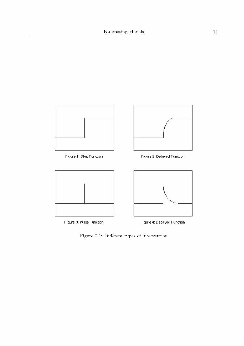
There are four different forms of intervention: step functions, delayed response, pulsefunctions, and decayed response. The simplest form is the step function. In the stepfunction the expectation of the influence of the intervention will be a sudden and lastingdecline or increase in the forecast output series. Suppose the intervention occurred at timeu. The dummy variable can be defined by

xt = s

{0 t < u1 t ≥ u

,

which is zero before the intervention and one after the intervention. This is called a ”stepintervention” because the graph of xt against t resembles a step, which can be seen inFigure 2.1. The intervention analysis model will then be given by

yt = a + ωxt + nt. (2.12)

Here yt denotes the output time series, xt denotes the input time series and nt is an ARIMAprocess. The value of ω represents the size or drop in the forecasting variable yt.

The other graphs of xt against t represent the remaining three types of intervention. Thesegraphs are shown in Figure 2.1. The names of the different types of intervention arechosen properly. They indicate the form of the graph. An extensive elaboration of theaforementioned types of intervention can be found in the book written by S. Makridakis,S.C. Wheelwright, and R.J. Hyndman [13].

Dynamic regression models (Transfer function models) are used in the article of Andrewsand Cunningham [1]. They used it to model the number of daily calls for orders (buyingmerchandize) and inquiries (e.g. checking order status) at L.L. Bean. In addition to theday of the week, covariates include the presence of holidays, catalogue mailings, as wellas forecasts for orders that are independently produced by the companys marketing de-partment. These periodic disruptions were modeled using intervention analysis along withother transfer functions to capture the effects of more regular influences.

Bianchi, Jarrett, and Hanumara [3] report in their article, that AT&T Bell Laboratories


Figure 2.1: Different types of intervention


used an adaptation of the Holt-Winters forecasting model with its telemarketing schedul-ing system, called NAMES for forecasting incoming calls in telemarketing centers. In theirstudy they try to evaluate the current use of the Holt-Winters model for forecasting asdone by the NAMES system and indicate whether improvement is possible through theuse of ARIMA time series modeling. The data they examined, revealed the presence ofoutliers, which was a big problem for the current NAMES software system. Interventionanalysis, the way in which ARIMA models can be used to account for outliers, performedsignificantly better than either of the Holt-Winters models in more than 50% of the timeseries studies. Five years later, Bianchi, Jarrett, and Hanumara [4] performed a similarstudy to analyze and improve existing methods for forecasting calls to telemarketing cen-ters for the purpose of planning and budgeting. The use of additive and multiplicativeversions of Holt-Winters exponentially weighted moving average models was analyzed andcompared to Box-Jenkins (ARIMA) modeling with intervention analysis. Once more, theyfound that ARIMA models with intervention analysis performed better for the time seriesstudied.

2.3 Exponential Smoothing

In the late 1950s exponential smoothing methods were developed for the first time by op-erations researchers. It is not clear whether Holt [10], Brown [7] or maybe even Magee [12]was the first to bring exponential smoothing. Since the development of this concept, itbecame a widely used method, partly due to its simplicity and low costs.

There are several exponential smoothing methods. The major ones used are Single Expo-nential Smoothing, Holt’s Linear Model (1957) and Holt-Winters’ Trend and SeasonalityModel. Subsequently, these methods will be described. An extensive elaboration on thesemodels may be found in Makradadis et al [13].

2.3.1 Single Exponential Smoothing

The simplest form of exponential smoothing is single exponential smoothing, and can onlybe used for data without any systematic trend or seasonal components. Given such a timeseries, a logical approach is to take a weighted average of past values. So for a seriesy1, y2, . . . , yt−1, the estimate of the value of yt, given the information available up to timet, is

yt = w0yt−1 + w1yt−2 + w2yt−3 + . . . ,

=inf∑i=0

wiyt−i+1, (2.13)

where wi are the weights given to the past values of the series and sum to one. Since themost recent observations of the series are also the most relevant, it is logical that these


observations should be given more weight than the observations further in the past. Thisis done by giving declining weights to the series. These decrease by a constant ratio andare of the form:

wi = α(1− α)i,

where i = 0, 1, 2, . . . and α is the smoothing constant in the range 0 < a < 1. For example,if α is set to 0.5, the weights will be:

w0 = 0.5,w1 = 0.25,w2 = 0.125,

....

The equation for the estimate of yt now becomes

yt = αyt−1 + α(1− α)yt−2 + α(1− α)2yt−3 + . . . , (2.14)

since

yt = αyt−1 + (1− α)(αyt−2 + α(1− α)yt−3 + . . .), (2.15)

it can be seen that

yt = αyt−1 + (1− α)yt−1. (2.16)

2.3.2 Holt’s Linear Model

Holt’s linear model is an extension of single exponential smoothing. Holt designed thismethod to allow forecasting of data with trends. The methods is as follows

For a time series y1, y2, . . . , yt−1, the estimate of the value of yt+u, is given by the nextformula

yt+u = mt + ubt u = 1, 2, . . . , (2.17)

where mt denotes an estimate of the level of the series at time t and bt denotes an estimateof the slope of the series at time t. The one step ahead formula is equal to

yt = mt−1 + bt−1, (2.18)

with the updating equations mt and bt as

mt = α0yt + (1− α0)(mt−1 + bt−1),

bt = α1(mt −mt−1) + (1− α1)bt−1, (2.19)

with 0 < α0 < 1 and 0 < α1 < 1.


2.3.3 Holt-Winters’ Trend and Seasonality Model

The exponential smoothing methods examined thus far can deal with almost any type ofdata as long as they are non-seasonal. Nevertheless, in case of seasonality these methods arenot very useful. Holt-winters’ trend and seasonality model can actually manage seasonality.

Holt’s linear model was extended by Winters[15] to include seasonality. The Holt-Winter’smethod is based on three smoothing equations: one for the level, one for the trend, andone for seasonality. It is similar to Holt’s model. The only difference is that an equationis added to deal with seasonality. In fact there are two different Holt-Winters’ methods.It depends on whether seasonality is modeled in an additive or multiplicative way. Thechoice of which to use depends on the characteristics of the specific time series. First themultiplicative model will be discussed.

Multiplicative Model The next formula gives the Holt-Winter’s multiplicative func-tion

yt+u = (mt + ubt)ct−s+u, (2.20)

where mt denotes the level of the time series at time t and bt represents the trend at timet. In this equation, the seasonal component is given by ct−s+u, with s as the length of theseasonal period, and yt+u the forecast for u periods ahead. For monthly data (s = 12), thenext formula is obtained

yt+1 = (mt + bt)ct−11. (2.21)

Because there are three components to exponential smoothing, three separate smoothingconstants are required. The first two constants were already known: α0 for the level, α1

for the slope. Now a third constant α2 is added for the seasonal component. The updatingequations of mt, bt and ct are respectively

mt = α0yt

ct−s

+ (1− α0)(mt−1 + bt−1),

bt = α1(mt −mt−1) + (1− α1)bt−1,

ct = α2yt

mt

+ (1− α2)ct−s, (2.22)

with α0, α1 and α2 between 0 and 1.

Additive Model The additive model is slightly different. Instead of multiplying theHolt model by the seasonal component, the seasonal factor is added. The formula willthen be given by

yt+u = mt + ubt + ct−s+u. (2.23)


Besides the difference mentioned before, the smoothing equations of mt and ct also differfrom those used in the multiplicative model. For perfection all the update equations areshown beneath.

mt = α0(yt − ct−s) + (1− α0)(mt−1 + bt−1),

bt = α1(mt −mt−1) + (1− α1)bt−1,

ct = α2(yt −mt) + (1− α2)ct−s. (2.24)

In only a few articles about forecasting call volumes at call centers, the exponential smooth-ing methods are discussed. In the article of W. Xu [16], she declared that exponentialsmoothing was one of the forecasting techniques implemented in Fedex’s major forecastingsoftware system (SAS). As described before Bianchi, Jarrett, and Hanumara [3] report intheir article, that AT&T Bell Laboratories used an adaptation of Holt-Winters forecastingmodel with its telemarketing scheduling system, called NAMES, for forecasting incomingcalls to telemarketing centers. Nevertheless, in their study to evaluate the current use of theHolt-Winters model for forecasting as done by the NAMES system and indicate whetherimprovement is possible through the use of ARIMA time series modeling. They foundARIMA models with intervention analysis to perform better for the time series studied. Intheir subsequent article, which was also discussed in the previous section, Bianchi, Jarrett,and Hanumara [4] performed a similar study to analyze existing and improved methods offorecasting calls to telemarketing centers for the purposes of planning and budgeting. Theuse of additive and multiplicative versions of Holt-Winters exponentially weighted movingaverage models was analyzed and compared to Box-Jenkins (ARIMA) modeling with in-tervention analysis. Once more, they found ARIMA models with intervention analysis toperform more effectively for the time series studied.

2.4 Regression Analysis

Another method used for forecasting call frequencies in call centers is regression analysis.A major advantage of the regression analysis is it is easier to understand, as will becomeclear below. A short description of regression analysis shall be presented. A completeoverview of regression analysis can be found in the book of Heij et al [9].

A regression analysis of time series is often categorized into three effects: the seasonaleffect, the trend effect and the random effect.

When time series are measured per quarter, per month, or even per day, they may containseasonal variation. The seasonal component in a time series refers to patterns that are re-peated over a one-year period and that average out in the long run. The patterns that donot average out are included in the constant and trend components of the model. Whereas


the trend is of dominant importance in long-term forecasting, the seasonal component isvery significant in short-term forecasting as it is often the main source of short-run fluc-tuations. Frequently, seasonal effects can be detected from plots of the time series, andalso from plots of the seasonal series that consist of the observations in the same month orquarter over different years.

The components can be added-up or multiplied. The models obtained are respectivelycalled the additive model and the multiplicative model. Both models are stated beneath

• multiplicativeyt = αsk

∗ βtk ∗ γrk,

• additiveyt = αsk

+ βtk + γrk,

where αskdenotes the factor determined by the influence of the season sk at time k, βtk

designates the factor determined by the influence of the trend tk at time k and γrkdes-

ignates the factor determined by the effect of the random component rk at time k. It ispossible to extend the equation. For instance, it is possible to include the daily effects,such as say the day of the week effect.

Because time series are divided into several components, textual documentation on thesubject often refer to it as time series decomposition. Of these pre-mentioned models themultiplicative model is the most widely applied, and often gives better predicting valuesthan the additive one.

It is possible to adopt the mentioned models in combination with linear regression. Beforethis model is given, first the theory of linear regression will be expounded concisely.

The most simple form of linear regression is simple linear regression. Simple linear re-gression is used in situations to evaluate the linear relationship between two variables.One example is the relationship between bank wages and education. In other words, sim-ple linear regression is used to develop an equation by which we can predict or estimate adependent variable (Bank wages), given an independent variable (education). The simpleregression equation is given by

y = a + bx, (2.25)

with y as the dependent variable, and a as the y intercept. The variable b is the gradientor slope of the line and x is the independent variable.

Sometimes it is needed to include more than one independent variable. For example,one might find out that if the variables education and initial salary are both included as


independent variables, the prediction of the dependent variable bank wages is much better.The term multiple regression denotes a number of independent variables that are included.The general formula of multiple regression is as follows

y = a +n∑

i=1

bixi, (2.26)

with y as the dependent variable, and a as the y intercept and xi for i = 1, . . . , n theindependent variables.

As mentioned before there is a possibility to apply decomposition of time series in com-bination with linear regression. If an additive time series decomposition is combined withmultiple regression the result is given by the next equation

yt = st + tt + rt + a +n∑

i=1

bixi. (2.27)

Articles about the prediction of call center call volumes show that regression analysis isnot frequently implemented method. In 1998, Klungle [11] tried to forecast the numberof incoming calls for the Emergency Road Service. They found this number to vary atdifferent times of the day significantly during winter and spring seasons. They also triedto model the incoming calls with the Holt-Winter’s method and a neural network method,but found that the regression analysis method performed best. Antipov and Meade [2]developed a forecasting model for the number of daily applications for loans at a financialservice telephone call center. They built a regression analysis model with a dynamic level,multiplicative calendar effects and a multiplicative advertising response. It was shown tobe more effective than an ARIMA model, which was used as a benchmark.

Chapter 3

Applying Techniques

It is now time to try one of the techniques described in the previous section. Becauseof the fact that the ARIMA model is the most widely applied model in the previous callcenter forecasting articles, this will be the first method adopted. The second method whichwill be adopted, is the Holt-winters’ trend and seasonality model. This method is chosenbecause of its simplicity and its speed.

Data is needed to forecast the call frequencies. Without data it is impossible to fit amodel, let alone to predict. In the first subsection a description will be given of the dataset used in this examination.

The prediction can be done using a software program, which can perform the compu-tations relatively fast, which are needed for the forecast. The software program includingthe add-ins are discussed in the subsection software.

To assess the results some measurements of forecasting accuracy must be determined.These measurements are explained shortly in the third subsection measurements of fore-casting accuracy.

The actual forecasting results will be placed in the fourth subsection results. Even thoughthese results have been gained with great devotion, there will always be possibilities forimprovement and further studies. Suggestions for possible improvements are provided inthe last section of this chapter.

3.1 Data

The data needed for the forecasts have been supplied by an insurance firm, which sellsits products to individuals as well as firms. The insurances they sell range from travelinsurances to life insurance policies.

19


Figure 3.1: Average week of car damage call volumes

As any other insurance company, it has a call center, which is used for both selling purposesand insurance claims. The examined database contained car damage call center frequen-cies. In the database, which was an Microsoft Excel file, the amount of calls were recordedfor every day in the past three years. The data ranges from Monday the 6th of January in2003 till Saturday the 22th of April in 2006.

Because the insurance company closes its call center on Sundays, the database only cap-tures call amounts from Monday till Saturday. Sometimes, call amounts of particular dayswere missing too. Most of these missing values are ascribed to National holidays, likeQueensday, Christmas, Easter, etc. Because these missing data could cause the predictingtechniques to fail, these data had to be filled in. The manner of assigning values to thegaps will be explained later on.

The data showed a strong seasonal effect within the week. Figure 3.1 displays the av-erage week of car damage call volumes. As can be seen from the figure, most calls come inon Monday. From Tuesday till Friday the amount of calls descend steadily. On Saturdaythe graph drops to its lowest point of the week, which is around 200 calls.

As mentioned before, the missing values had to be compensated. As the figure displayed,the particular day of the week is a very important factor. Thus, the missing values were tobe appointed with care. The manner to compensate for these missing values, was to take

Applying Techniques 21

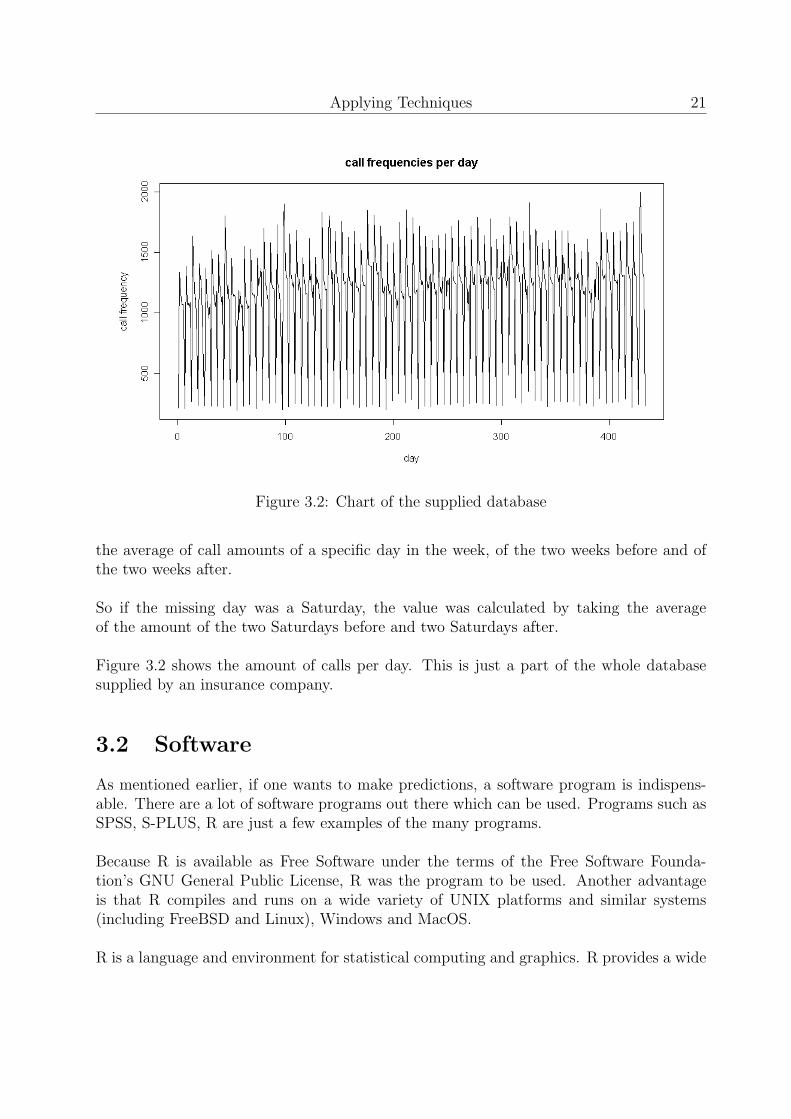
Figure 3.2: Chart of the supplied database

the average of call amounts of a specific day in the week, of the two weeks before and ofthe two weeks after.

So if the missing day was a Saturday, the value was calculated by taking the averageof the amount of the two Saturdays before and two Saturdays after.

Figure 3.2 shows the amount of calls per day. This is just a part of the whole databasesupplied by an insurance company.

3.2 Software

As mentioned earlier, if one wants to make predictions, a software program is indispens-able. There are a lot of software programs out there which can be used. Programs such asSPSS, S-PLUS, R are just a few examples of the many programs.

Because R is available as Free Software under the terms of the Free Software Founda-tion’s GNU General Public License, R was the program to be used. Another advantageis that R compiles and runs on a wide variety of UNIX platforms and similar systems(including FreeBSD and Linux), Windows and MacOS.

R is a language and environment for statistical computing and graphics. R provides a wide


variety of statistical (linear and nonlinear modeling, classical statistical tests, time-seriesanalysis, classification, clustering, ...) and graphical techniques, and is highly extensible.More information about R can be found at the site

http://cran.r-project.org.

Within R it is possible to write your own extensions and functions. Due to this and thefact that R is Open Source, a lot of extensions and functions written by others can befound on the internet.

The forecasts made in this examination are made using self-written functions. Theseself-written functions were based partly based on an extension and partly based on built-infunctions.

In R extensions are called packages. The used package for the forecasts of the ARIMAmethod, the first predicting technique, is written by Rob J. Hyndman and is given thename forecast. It includes all kinds of convenient forecast functions. If one is interested,information about the package and the package itself can be downloaded from the site

http://www-personal.buseco.monash.edu.au/ hyndman/Rlibrary/forecast/.

The functions of the forecast package, which were used for forecasting the call frequencieswith the ARIMA method, were best.arima() and forecast().

As previously told in the ARIMA model section, the order of the model(p,d,q) has tobe selected before the predicting phase can begin. The selection of the right order ismainly based on the AIC (Akaike Information Criterion). This AIC should be minimized.The model which has the minimal AIC is considered the best model. Searching for thisminimal AIC value is mainly a trial and error process and can go on forever.

The function best.arima() automates this exhaustive search, it looks as the name indi-cates for the best ARIMA model. At the moment best.arima() found the best model, thefunction forecast() can begin producing the forecasts using this model. It should be men-tioned though, this whole process can take hours. Naturally, this is partly dependent onthe computer’s built-in CPU. The average run in this examination took at least ten hours.

The functions used for the second predicting technique, Holt-winters’ trend and seasonalitymodel, were already in R. These functions were ts(), HoltWinters(), and predict().

ts() is a function, used for mutating the database into time series. The function HoltWin-ters() fits the model to the data and predict() is used for calculating the actual predictionsusing the model returned by the HoltWinters() function.

If one is interested, one can find all the self-written R-code in the Appendix.


3.3 Measurements of Forecasting Accuracy

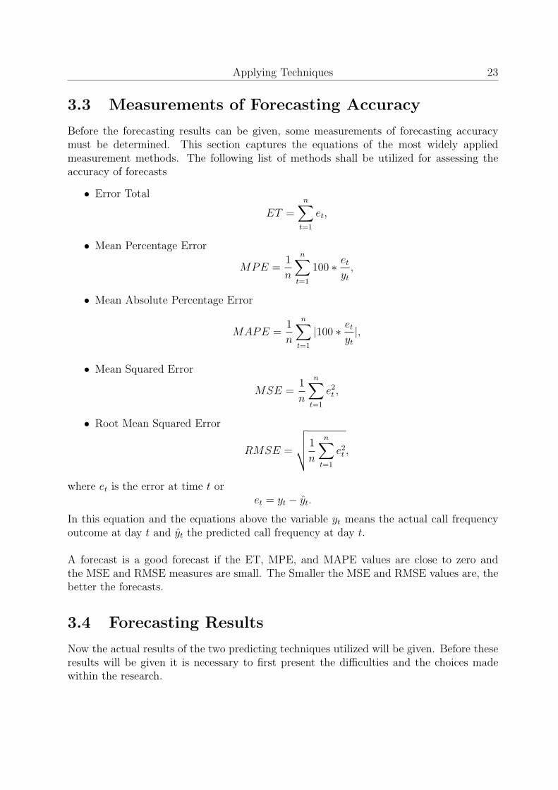
Before the forecasting results can be given, some measurements of forecasting accuracymust be determined. This section captures the equations of the most widely appliedmeasurement methods. The following list of methods shall be utilized for assessing theaccuracy of forecasts

• Error Total

ET =n∑

t=1

et,

• Mean Percentage Error

MPE =1

n

n∑t=1

100 ∗ et

yt

,

• Mean Absolute Percentage Error

MAPE =1

n

n∑t=1

|100 ∗ et

yt

|,

• Mean Squared Error

MSE =1

n

n∑t=1

e2t ,

• Root Mean Squared Error

RMSE =

√√√√ 1

n

n∑t=1

e2t ,

where et is the error at time t oret = yt − yt.

In this equation and the equations above the variable yt means the actual call frequencyoutcome at day t and yt the predicted call frequency at day t.

A forecast is a good forecast if the ET, MPE, and MAPE values are close to zero andthe MSE and RMSE measures are small. The Smaller the MSE and RMSE values are, thebetter the forecasts.

3.4 Forecasting Results

Now the actual results of the two predicting techniques utilized will be given. Before theseresults will be given it is necessary to first present the difficulties and the choices madewithin the research.


The first choice made, was to predict the daily call frequencies using 630 data points.This means that both predicting techniques would be fitted to 630 daily call volume data.The choice to fit to 630 data points was made, due to the fact that 630 call frequenciesmake exactly two years of data. Two years is just good enough to find a good model,and at the same time it is not too long. This way the history will not have too great aninfluence. Eventually, this will improve the quality of the forecasts.

To compute the precise forecast accuracy predictions have to be made over a long period.The longer this period is, the more accurate the forecast errors are. In this examination,the forecasts are 312 days long, which is long enough to provide precise forecast accuracynumbers.

The forecasts could be done in different ways, which means there were several variablesthat could be adapted. Within the ARIMA predicting method, one of those adaptionswas the amount of times best.arima() got the assignment to calculate. For example, thechoice could be made that best.arima() computed the best order ARIMA model once in aweek and that this model would be exploited self-evidently for the predictions of one week.However, it was also possible for best.arima() to calculate the best model each day, whichwould then be exploited for the prediction of only one day.

The same was found for the Holt-Winters’ trend and seasonality prediction model. Onlywithin the Holt-Winters’ method the function Holt-Winters() was called for computing thebest fitting model. So, decisions had to be made about the amount of times the functionHoltWinters() was called.

Another variable was the moment of time the prediction was made. For example, it ispossible to produce today the forecasts for the next month. Another option is to producethe forecasts today for tomorrow. Because the main purpose of the prediction is to sched-ule the right amount of personnel, the moment of time is taken into consideration. Thehighest prediction accuracy would probably be reached by predicting one day in advance.But call center employees will certainly not accept this. Maybe the flexible student hassome interest in working in this way, but the average worker wants to have some securityin his/her live and wants to know when he/she has to work weeks in advance. The as-sumption is made that schedules will be accepted by employees if they are presented tothem at least two weeks in advance.

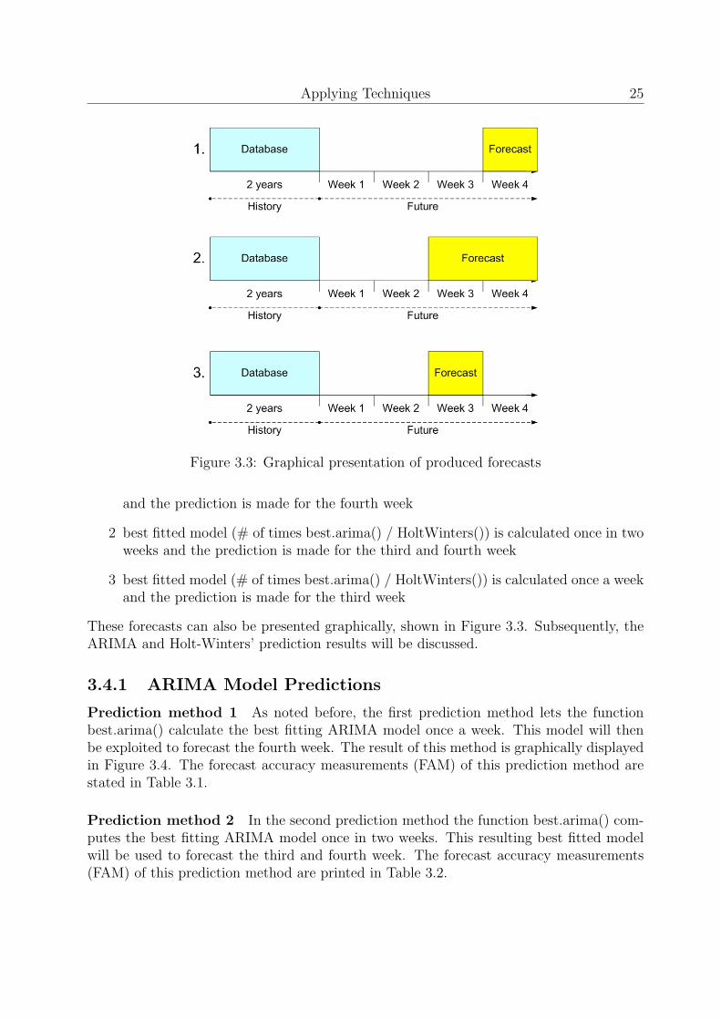
As previously mentioned, forecasting with the ARIMA method is time consuming. Thusit was necessary to make some choices about the pre-mentioned variables and the amountof forecasts. There has been chosen to perform three forecasts for each prediction method.These forecasts are listed below.

1 best fitted model (# of times best.arima() / HoltWinters()) is calculated once a week


Figure 3.3: Graphical presentation of produced forecasts

and the prediction is made for the fourth week

2 best fitted model (# of times best.arima() / HoltWinters()) is calculated once in twoweeks and the prediction is made for the third and fourth week

3 best fitted model (# of times best.arima() / HoltWinters()) is calculated once a weekand the prediction is made for the third week

These forecasts can also be presented graphically, shown in Figure 3.3. Subsequently, theARIMA and Holt-Winters’ prediction results will be discussed.

3.4.1 ARIMA Model Predictions

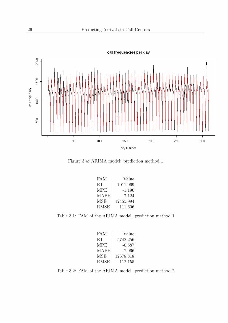
Prediction method 1 As noted before, the first prediction method lets the functionbest.arima() calculate the best fitting ARIMA model once a week. This model will thenbe exploited to forecast the fourth week. The result of this method is graphically displayedin Figure 3.4. The forecast accuracy measurements (FAM) of this prediction method arestated in Table 3.1.

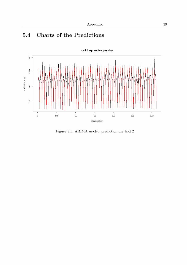
Prediction method 2 In the second prediction method the function best.arima() com-putes the best fitting ARIMA model once in two weeks. This resulting best fitted modelwill be used to forecast the third and fourth week. The forecast accuracy measurements(FAM) of this prediction method are printed in Table 3.2.


Figure 3.4: ARIMA model: prediction method 1

FAM ValueET -7011.069MPE -1.190MAPE 7.124MSE 12455.994RMSE 111.606

Table 3.1: FAM of the ARIMA model: prediction method 1




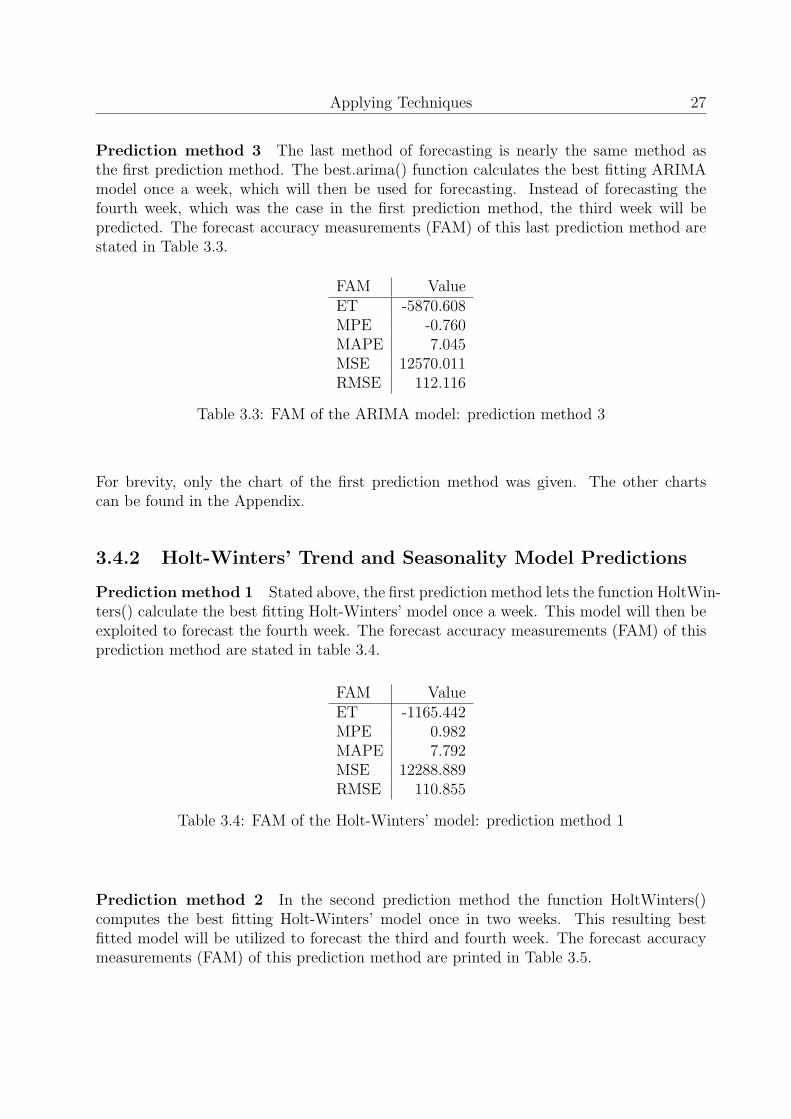
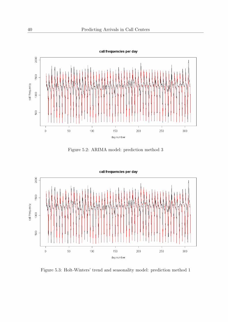
Prediction method 3 The last method of forecasting is nearly the same method asthe first prediction method. The best.arima() function calculates the best fitting ARIMAmodel once a week, which will then be used for forecasting. Instead of forecasting thefourth week, which was the case in the first prediction method, the third week will bepredicted. The forecast accuracy measurements (FAM) of this last prediction method arestated in Table 3.3.



For brevity, only the chart of the first prediction method was given. The other chartscan be found in the Appendix.

3.4.2 Holt-Winters’ Trend and Seasonality Model Predictions

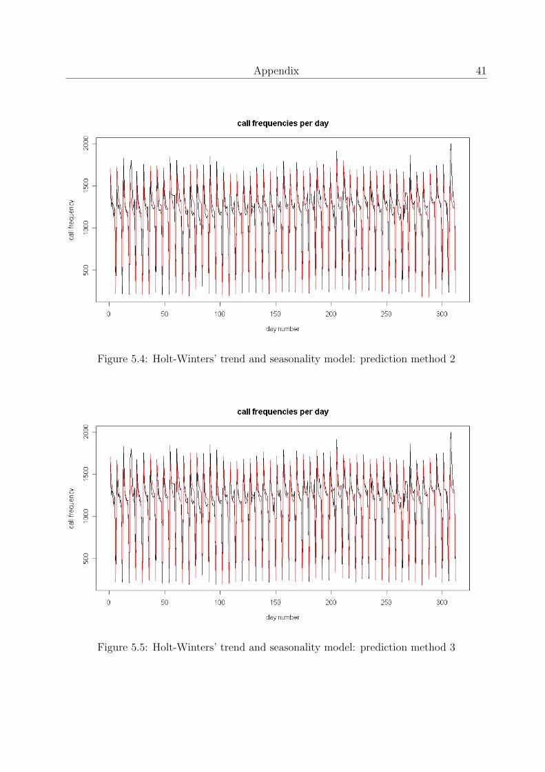
Prediction method 1 Stated above, the first prediction method lets the function HoltWin-ters() calculate the best fitting Holt-Winters’ model once a week. This model will then beexploited to forecast the fourth week. The forecast accuracy measurements (FAM) of thisprediction method are stated in table 3.4.

FAM ValueET -1165.442MPE 0.982MAPE 7.792MSE 12288.889RMSE 110.855

Table 3.4: FAM of the Holt-Winters’ model: prediction method 1

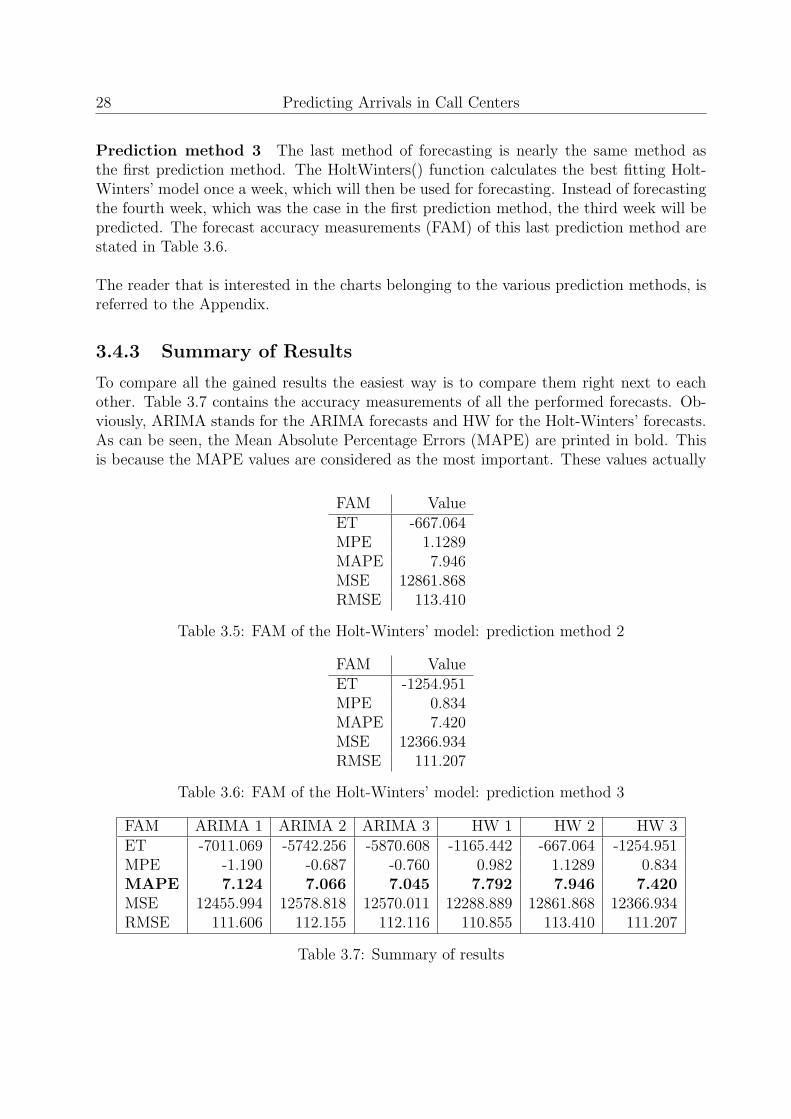
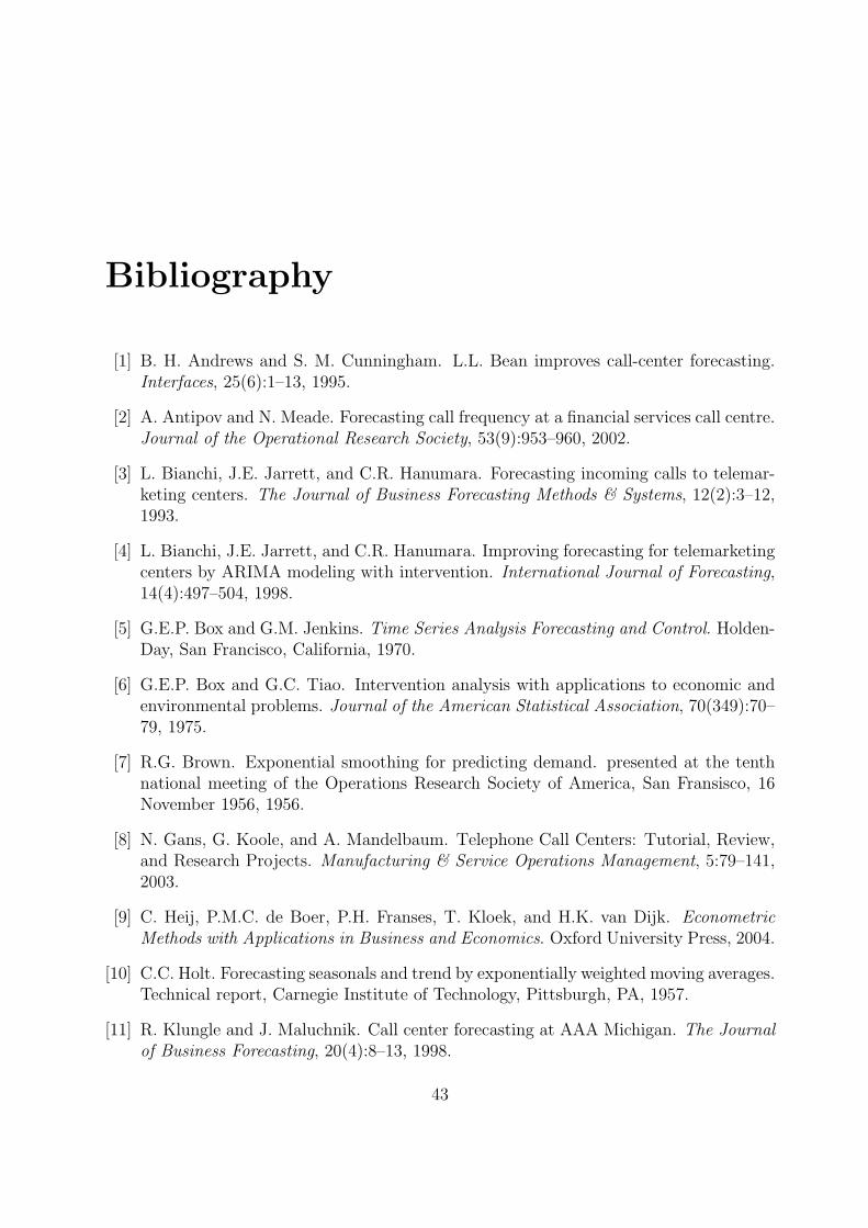
Prediction method 2 In the second prediction method the function HoltWinters()computes the best fitting Holt-Winters’ model once in two weeks. This resulting bestfitted model will be utilized to forecast the third and fourth week. The forecast accuracymeasurements (FAM) of this prediction method are printed in Table 3.5.


Prediction method 3 The last method of forecasting is nearly the same method asthe first prediction method. The HoltWinters() function calculates the best fitting Holt-Winters’ model once a week, which will then be used for forecasting. Instead of forecastingthe fourth week, which was the case in the first prediction method, the third week will bepredicted. The forecast accuracy measurements (FAM) of this last prediction method arestated in Table 3.6.

The reader that is interested in the charts belonging to the various prediction methods, isreferred to the Appendix.

3.4.3 Summary of Results

To compare all the gained results the easiest way is to compare them right next to eachother. Table 3.7 contains the accuracy measurements of all the performed forecasts. Ob-viously, ARIMA stands for the ARIMA forecasts and HW for the Holt-Winters’ forecasts.As can be seen, the Mean Absolute Percentage Errors (MAPE) are printed in bold. Thisis because the MAPE values are considered as the most important. These values actually





FAM ARIMA 1 ARIMA 2 ARIMA 3 HW 1 HW 2 HW 3ET -7011.069 -5742.256 -5870.608 -1165.442 -667.064 -1254.951MPE -1.190 -0.687 -0.760 0.982 1.1289 0.834MAPE 7.124 7.066 7.045 7.792 7.946 7.420MSE 12455.994 12578.818 12570.011 12288.889 12861.868 12366.934RMSE 111.606 112.155 112.116 110.855 113.410 111.207

Table 3.7: Summary of results


tell the deviation of the predictions in relation to the actual outcome values. According tothe table, the third prediction with the ARIMA model is the most accurate, albeit thereis not a big difference with the other ARIMA predictions. The MAPE values of ARIMAare much lower than the values of Holt-Winters’.

A big difference can be seen in The Error Total (ET) measurements between the ARIMAmethod forecasts and the Holt-Winters’ forecasts. The ET values of the Holt-Winters’forecasts are significantly lower than the ARIMA method forecasts. This means that thedaily call frequency predictions of the ARIMA method are often below the actual outcomes.Thus, the call frequencies are predicted too low. The ET values of the Holt-Winter’s fore-casts are closer to zero, which is somewhat better.

In the remaining results there was no other clear difference between the ARIMA andHolt-Winters’ methods. The Mean Percentage Error (MPE) values are all close to zero,which is the value it should have. The Mean Squared Error (MSE) is continuously aroundthe 12,500 and the Root Mean Squared Error (RMSE), which is deducted from the MSEis around the 112.

As mentioned earlier, the MAPE value is the leading measurement. According to theMAPE value the third forecast made with ARIMA is the most accurate one, notwithstand-ing the fact that there is no big difference with the other ARIMA predictions. Striking isthe fact that the ARIMA forecasts all have better MAPE values than the Holt-Winters’forecasts. On the other hand, it is not that surprising. The average computation timeneeded for the ARIMA forecasts was about ten hours, while the calculations of all theforecasts with the Holt-Winters’ model were done within 1 minute. According to thecomputing effort and the time invested, the ARIMA model should give better predictions.

3.5 Suggestions for Improvement

As has become clear in the previous sections, some choices needed to be made. This wasmainly because of the fact that best.arima() required a lot of time to find the best ARIMAmodel. In spite of all the efforts made and the time that has been contributed to this study,there are some possibilities for improvement. First, one could adjust the time to prediction.In this examination the predictions were made two or three weeks in advance. For exam-ple, it is a possibility to make the predictions just one week in advance. In other words,one could predict the second week instead of the third and fourth, which were done in thisexamination. Predicting the second week will by all odds result in better prediction values.

Second, one could compute the best fitted ARIMA order model every day. In this study,best.arima() calculated the best model only once a week or once in two weeks. In this caseit is not clear if this suggestion will actually be an improvement, but it is certainly worthtrying. A warning should be made to the reader; this calculation would probably take you


60 hours!

Third, the attributes given to the function best.arima() could be changed. The ARIMAforecasts produced in this examination all used the next call

> best.arima("database", max.p = 10,stationary=TRUE, max.q = 10,

max.order=30)

This means that best.arima() searched for the best fitted ARIMA(p,d,q) model, while sat-isfying the requirements to search only for models, which satisfy the equations p ≤ 10,d ≤ 10, and q ≤ 10. Possibly, changing these requirements to p ≤ 15, d ≤ 15, and q ≤ 15would give more accurate forecasts, but then again the computing time would increaseexponentially.

Once again, the reader who wishes to forecast and make these possible improvements,should have a computer with an immense computing speed or an enormous load of freetime.

Chapter 4

Conclusions and Further Research

The question is which of the aforementioned models to use for forecasting. Actually thereis no single best forecasting model. Each model may be best fitted into a specific situation.In this section the advantages/disadvantages will be described of each model.

ARIMA Model The short-term forecasts of the ARIMA model are more reliable thanthe long-term forecasts. This is because of the fact that the emphasis in forecasts is onshort-term forecasting. ARIMA models namely place heavy emphasis on the recent pastrather than the distant past.

One of the most important disadvantages for the ARIMA modeling approach is the ne-cessity of a large amount of data. Without a large amount of call center call frequencyrecordings ARIMA does not function well.

Another disadvantage of this modeling approach is that it is a complex technique, whichrequires a great deal of experience and although it often produces satisfactory results,those results depend on the researcher’s level of expertise, for ARIMA model building is anempirically driven methodology of systematically identifying, estimating, diagnosing, andforecasting time series. This cycle of model building continuously requires the presenceand judgement of expert analysts, which can be very expensive.

The computing time needed for the ARIMA model is longer than most of the aforemen-tioned forecasting techniques. For purposes, which need a quick and reliable forecast,ARIMA is not the appropriate model to exploit.

Though these disadvantages might give the feeling ARIMA is not the most ideal fore-casting model, ARIMA is capable of producing outstandingly good predictions, which iscertainly worth trying.

Dynamic Regression Models Dynamic regression models are actually extensions ofthe ARIMA model and deal with the shortcomings of the ARIMA model. So the same ad-

31


vantages / disadvantages described in the previous paragraph bear on dynamic regressionmodels.

The ARIMA model discussed in the previous section deals with single time series anddoes not allow the inclusion of other information in the models and forecasts. However,frequently other information may be used to aid in forecasting time series. Informationabout holidays, strikes, changes in the law, or other external variables may be of use inassisting the development of more accurate forecasts. Dynamic regression models offer thepossibility to include this information, which is a clear advantage.

Exponential Smoothing Also with exponential smoothing models heavy emphasis isplaced on the recent past rather than the distant past. So short-term forecasts of expo-nential smoothing models are more reliable than the long-term forecasts.

The major advantages of widely used smoothing methods are their simplicity and lowcost. Its forecasting equations are easily interpreted and understood by management. Soit is popular in call center call volume forecasting systems.

The origin of low costs lies in the fact that exponential smoothing methods are simpleto use and can be applied almost automatically. The attendance of expert analysts is thuskept to a minimum. Besides this, the computing time needed to calculate the forecasts isnegligible.

A major disadvantage of exponential smoothing methods, is its sensibility to outliers.Outliers can have dramatic effects on forecasts, and should be eliminated.

Self-evidently the disadvantage of single exponential smoothing is that it only works forno trend and no seasonality patterns. Holt’s linear models’ shortcoming is its disability tomanage seasonality. Nevertheless, Holt-Winters’ trend and seasonality model can managetrends and seasonality and thus solves the inadequacies of the other exponential smoothingmethods.

It is possible that better accuracy can be obtained using more sophisticated methods,such as ARIMA. However, when forecasts are needed for an incredibly amount of items,as is the case in many inventory systems, smoothing methods are often the only methodsthat are fast enough for acceptable implementation.

Regression Analysis The main disadvantage of regression analysis is that it is hard toimplement in an automatic modeling system. It may face multicollinearity problems, serialcorrelation problems, heteroscedasticity problems, etc. which need bunches of tests withhuman judgments. Through the inference of expert analysts the costs shall increase, bywhich this method will not belong to the most economical ones.

Conclusions and Further Research 33

The process of building the right forecast model is the most time swallowing part. Once amodel is obtained, the computation efforts will be negligible.

Though this description might give a negative impression, this model can give outstand-ingly good predictions.

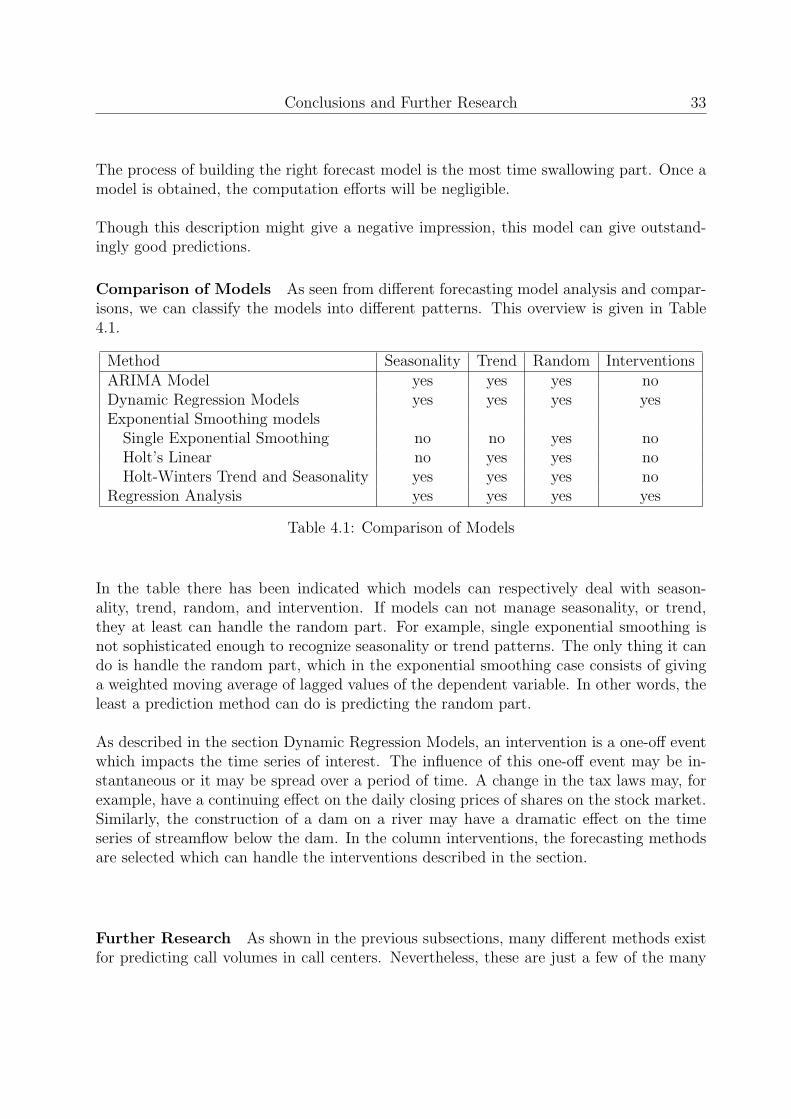
Comparison of Models As seen from different forecasting model analysis and compar-isons, we can classify the models into different patterns. This overview is given in Table4.1.

Method Seasonality Trend Random InterventionsARIMA Model yes yes yes noDynamic Regression Models yes yes yes yesExponential Smoothing models

Single Exponential Smoothing no no yes noHolt’s Linear no yes yes noHolt-Winters Trend and Seasonality yes yes yes no

Regression Analysis yes yes yes yes

Table 4.1: Comparison of Models

In the table there has been indicated which models can respectively deal with season-ality, trend, random, and intervention. If models can not manage seasonality, or trend,they at least can handle the random part. For example, single exponential smoothing isnot sophisticated enough to recognize seasonality or trend patterns. The only thing it cando is handle the random part, which in the exponential smoothing case consists of givinga weighted moving average of lagged values of the dependent variable. In other words, theleast a prediction method can do is predicting the random part.

As described in the section Dynamic Regression Models, an intervention is a one-off eventwhich impacts the time series of interest. The influence of this one-off event may be in-stantaneous or it may be spread over a period of time. A change in the tax laws may, forexample, have a continuing effect on the daily closing prices of shares on the stock market.Similarly, the construction of a dam on a river may have a dramatic effect on the timeseries of streamflow below the dam. In the column interventions, the forecasting methodsare selected which can handle the interventions described in the section.

Further Research As shown in the previous subsections, many different methods existfor predicting call volumes in call centers. Nevertheless, these are just a few of the many


possible forecasting methods. As correctly stated by Gans, Koole and Mandelbaum [8] thepractice of time series forecasting at call centers is ”still in its infancy”. There are manymethods for making quantitative forecasts which have not been applied to call centerdata. For instance, it is possible to extent ARIMA to include seasonal effects (SARIMA).SARIMA has already been applied successfully to predict the consumption of goods bycivilians and the urban freeway traffic flow. Another possibility is to use the State Spacemodels methodology, which is also applied to predict urban freeway traffic flow.

Neural Networks are increasingly used for quantitative prediction purposes. The appli-cations of this artificial forecasting method are endless. For example, it is useful in deter-mining rainfall expectations, the performance of the stock prices, and the short-term loadof electrical engineering.

These models form merely a fraction of the models that can possibly be used for fore-casting call volumes in call centers. Extensive research shall point out if these models canbe utilized successfully.

Chapter 5

Appendix

5.1 ARIMA Functions R-code

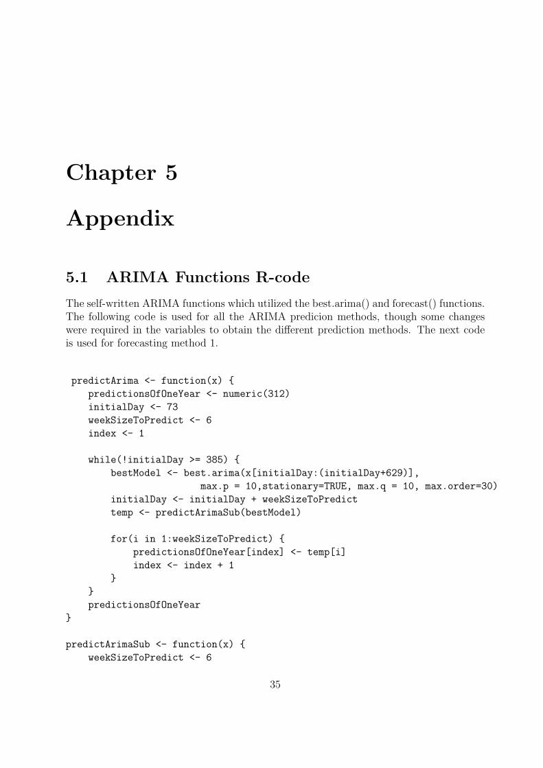
The self-written ARIMA functions which utilized the best.arima() and forecast() functions.The following code is used for all the ARIMA predicion methods, though some changeswere required in the variables to obtain the different prediction methods. The next codeis used for forecasting method 1.

predictArima <- function(x) {

predictionsOfOneYear <- numeric(312)

initialDay <- 73

weekSizeToPredict <- 6

index <- 1

while(!initialDay >= 385) {

bestModel <- best.arima(x[initialDay:(initialDay+629)],

max.p = 10,stationary=TRUE, max.q = 10, max.order=30)

initialDay <- initialDay + weekSizeToPredict

temp <- predictArimaSub(bestModel)

for(i in 1:weekSizeToPredict) {

predictionsOfOneYear[index] <- temp[i]

index <- index + 1

}

}

predictionsOfOneYear

}

predictArimaSub <- function(x) {


35


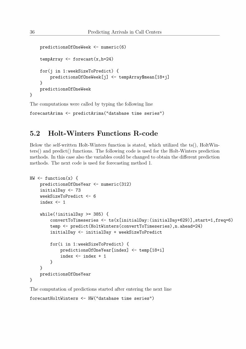
predictionsOfOneWeek <- numeric(6)

tempArray <- forecast(x,h=24)

for(j in 1:weekSizeToPredict) {

predictionsOfOneWeek[j] <- tempArray$mean[18+j]

}

predictionsOfOneWeek

}

The computations were called by typing the following line

forecastArima <- predictArima("database time series")

5.2 Holt-Winters Functions R-code

Below the self-written Holt-Winters function is stated, which utilized the ts(), HoltWin-ters() and predict() functions. The following code is used for the Holt-Winters predictionmethods. In this case also the variables could be changed to obtain the different predictionmethods. The next code is used for forecasting method 1.

HW <- function(x) {

predictionsOfOneYear <- numeric(312)

initialDay <- 73


index <- 1

while(!initialDay >= 385) {

convertToTimeseries <- ts(x[initialDay:(initialDay+629)],start=1,freq=6)

temp <- predict(HoltWinters(convertToTimeseries),n.ahead=24)

initialDay <- initialDay + weekSizeToPredict

for(i in 1:weekSizeToPredict) {

predictionsOfOneYear[index] <- temp[18+i]

index <- index + 1

}

}

predictionsOfOneYear

}

The computation of predictions started after entering the next line

forecastHoltWinters <- HW("database time series")

Appendix 37

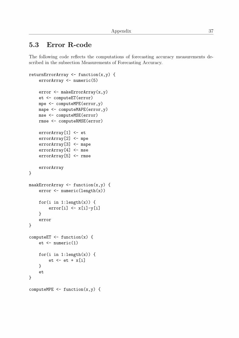
5.3 Error R-code

The following code reflects the computations of forecasting accuracy measurements de-scribed in the subsection Measurements of Forecasting Accuracy.

returnErrorArray <- function(x,y) {

errorArray <- numeric(5)

error <- makeErrorArray(x,y)

et <- computeET(error)

mpe <- computeMPE(error,y)

mape <- computeMAPE(error,y)

mse <- computeMSE(error)

rmse <- computeRMSE(error)

errorArray[1] <- et

errorArray[2] <- mpe

errorArray[3] <- mape

errorArray[4] <- mse

errorArray[5] <- rmse

errorArray

}

maakErrorArray <- function(x,y) {

error <- numeric(length(x))

for(i in 1:length(x)) {

error[i] <- x[i]-y[i]

}

error

}

computeET <- function(x) {

et <- numeric(1)


et <- et + x[i]

}

et

}

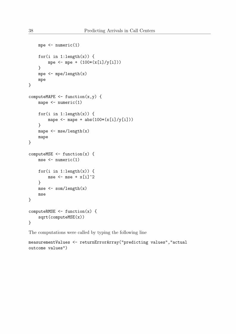
computeMPE <- function(x,y) {


mpe <- numeric(1)


mpe <- mpe + (100*(x[i]/y[i]))

}

mpe <- mpe/length(x)

mpe

}

computeMAPE <- function(x,y) {

mape <- numeric(1)


mape <- mape + abs(100*(x[i]/y[i]))

}

mape <- mse/length(x)

mape

}

computeMSE <- function(x) {

mse <- numeric(1)


mse <- mse + x[i]^2

}

mse <- som/length(x)

mse

}

computeRMSE <- function(x) {

sqrt(computeMSE(x))

}

The computations were called by typing the following line

measurementValues <- returnErrorArray("predicting values","actual

outcome values")

Appendix 39

5.4 Charts of the Predictions




Figure 5.3: Holt-Winters’ trend and seasonality model: prediction method 1

Appendix 41



Bibliography

[1] B. H. Andrews and S. M. Cunningham. L.L. Bean improves call-center forecasting.Interfaces, 25(6):1–13, 1995.

[2] A. Antipov and N. Meade. Forecasting call frequency at a financial services call centre.Journal of the Operational Research Society, 53(9):953–960, 2002.

[3] L. Bianchi, J.E. Jarrett, and C.R. Hanumara. Forecasting incoming calls to telemar-keting centers. The Journal of Business Forecasting Methods & Systems, 12(2):3–12,1993.

[4] L. Bianchi, J.E. Jarrett, and C.R. Hanumara. Improving forecasting for telemarketingcenters by ARIMA modeling with intervention. International Journal of Forecasting,14(4):497–504, 1998.

[5] G.E.P. Box and G.M. Jenkins. Time Series Analysis Forecasting and Control. Holden-Day, San Francisco, California, 1970.

[6] G.E.P. Box and G.C. Tiao. Intervention analysis with applications to economic andenvironmental problems. Journal of the American Statistical Association, 70(349):70–79, 1975.

[7] R.G. Brown. Exponential smoothing for predicting demand. presented at the tenthnational meeting of the Operations Research Society of America, San Fransisco, 16November 1956, 1956.

[8] N. Gans, G. Koole, and A. Mandelbaum. Telephone Call Centers: Tutorial, Review,and Research Projects. Manufacturing & Service Operations Management, 5:79–141,2003.

[9] C. Heij, P.M.C. de Boer, P.H. Franses, T. Kloek, and H.K. van Dijk. EconometricMethods with Applications in Business and Economics. Oxford University Press, 2004.

[10] C.C. Holt. Forecasting seasonals and trend by exponentially weighted moving averages.Technical report, Carnegie Institute of Technology, Pittsburgh, PA, 1957.

[11] R. Klungle and J. Maluchnik. Call center forecasting at AAA Michigan. The Journalof Business Forecasting, 20(4):8–13, 1998.

43


[12] J.F. Magee. Production Planning and Inventory Control. McGraw-Hill, New York.

[13] S. Makridakis, S.C. Wheelwright, and R.J. Hyndman. Forecasting: Methods andApplications. John Wiley and Sons, Inc., 1998.

[14] J. Nijdam. Forecasting telecommunications services using Box-Jenkins (ARIMA) mod-els. Telecommunication Journal of Australia, 40(1):31–37.

[15] P.R. Winters. Forecasting sales by exponentially weigthed moving averages. Manage-ment Science, 6:324–342, 1960.

[16] Weidong Xu. Longe range planning for call centers at FedEx. The Journal of BusinessForecasting Methods and Systems, 18(4):7–11, Winter 1999/2000.

predicting call arrivals in call centers · predicting call arrivals in call centers koen van den...

Documents