predictability of hydrologic response at the plot and ... · predictability of hydrologic response...

Predictability of hydrologic response at the plot

and catchment scales: Role of initial conditions

Erwin Zehe

Institute of Geoecology, University of Potsdam, Potsdam, Germany

Gunter Bloschl

Institute of Hydraulics, Hydrology and Water Resources Management, Vienna University of Technology, Vienna, Austria

Received 7 November 2003; revised 1 April 2004; accepted 12 August 2004; published 1 October 2004.

[1] This paper examines the effect of uncertain initial soil moisture on hydrologicresponse at the plot scale (1 m2) and the catchment scale (3.6 km2) in the presence ofthreshold transitions between matrix and preferential flow. We adopt the concepts ofmicrostates and macrostates from statistical mechanics. The microstates are the detailedpatterns of initial soil moisture that are inherently unknown, while the macrostates arespecified by the statistical distributions of initial soil moisture that can be derived from themeasurements typically available in field experiments. We use a physically based modeland ensure that it closely represents the processes in the Weiherbach catchment, Germany.We then use the model to generate hydrologic response to hypothetical irrigationevents and rainfall events for multiple realizations of initial soil moisture microstates thatare all consistent with the same macrostate. As the measures of uncertainty at the plot scalewe use the coefficient of variation and the scaled range of simulated vertical bromidetransport distances between realizations. At the catchment scale we use similar statisticsderived from simulated flood peak discharges. The simulations indicate that at bothscales the predictability depends on the average initial soil moisture state and is at aminimum around the soil moisture value where the transition from matrix to macroporeflow occurs. The predictability increases with rainfall intensity. The predictabilityincreases with scale with maximum absolute errors of 90 and 32% at the plot scale and thecatchment scale, respectively. It is argued that even if we assume perfect knowledge on theprocesses, the level of detail with which one can measure the initial conditions along withthe nonlinearity of the system will set limits to the repeatability of experiments andlimits to the predictability of models at the plot and catchment scales. INDEX TERMS: 1866

Hydrology: Soil moisture; 1860 Hydrology: Runoff and streamflow; 1875 Hydrology: Unsaturated zone;

KEYWORDS: flood response, hydrological model, predictability, preferential flow, scale

Citation: Zehe, E., and G. Bloschl (2004), Predictability of hydrologic response at the plot and catchment scales: Role of initial

conditions, Water Resour. Res., 40, W10202, doi:10.1029/2003WR002869.

1. Introduction

[2] Understanding and modeling hydrologic systemresponse at different scales is hampered by an often poorreproducibility of plot-scale and catchment-scale experi-ments. The same set of measured parameters, state variablesand boundary conditions can often be associated withmarkedly different system responses. Lischeid et al.[2000], for example, observed tracer velocities between30.6 and 10.6 m d�1 during three identical steady statefield-scale breakthrough experiments at the Gardsjon testcatchment. The differences could not be related to anymeasurable difference in the experimental conditions.Investigating field-scale tracer transport, Lennartz et al.[1999] showed that for their highly macroporous soil itwas not possible to predict whether preferential flow willoccur or not, even though they had obtained very detailed

measurements of soil parameters and the moisture state.When one moves up to larger scales the same problemprevails. As lucidly discussed by Beven [2000], no matterwhat is the sophistication of a physically based model therewill always be a large degree of uncertainty in the predic-tions which will be difficult to account for. This uncertaintylimits the predictability of hydrologic response.[3] There have been a number of alternative explanations

for the sources of this uncertainty in the hydrologic litera-ture over the years. These include parameter uncertainty[Wood, 1976], uncertainty in the model structure [Beven,1989], and uncertainty in the input data and initial con-ditions [Grayson and Bloschl, 2000]. A recent workshopreport on challenges in hydrologic predictability noted[National Research Council (NRC), 2003, p. 17] ‘‘inwatershed rainfall-runoff transformation. . .initial andboundary conditions are the critical issues.’’ This variableassessment raises an interesting question of whether thedetailed measurements typically available in research catch-ments would constrain the system state enough to give

Copyright 2004 by the American Geophysical Union.0043-1397/04/2003WR002869$09.00

W10202

WATER RESOURCES RESEARCH, VOL. 40, W10202, doi:10.1029/2003WR002869, 2004

1 of 21

unique predictions of hydrologic response, assuming perfectknowledge on the nature of the processes (as represented bythe structure and parameters of a model). Clearly, this willdepend on the level of detail of the field measurements but,no matter how detailed the measurements are, there willalways be points in space where we do not have measure-ments, so there will always be a smaller-scale component ofhydrologic variability that will not be captured by the data.This small-scale component may or may not become impor-tant in controlling hydrologic response. This is the uncer-tainty this paper examines with a focus on initial conditions.[4] The degree to which field measurement constrain the

catchment state in terms of producing a unique responsewill also depend on the degree and type of nonlinearity ofthe underlying processes. Certain types of nonlinearity leadto chaotic behavior of the system which amplifies uncer-tainties and limits predictability significantly [Gleick, 1993;Sivakumar, 2000]. In this paper we examine thresholdbehavior which is one particular form of process non-linearity. There are a number of threshold processes inhydrology where the system switches between different‘‘dynamic regimes.’’ An obvious example of two differentregimes is wet and dry periods of rainfall. Similarly,evaporation may be subject to different regimes, eithercontrolled by atmospheric demand or by soil hydraulicproperties [Dooge, 1986]. Snowmelt and freezing are typ-ical threshold processes. Another example is surface runoffgeneration which is often conceptualized as a thresholdprocess. If rainfall intensity exceeds infiltration capacitysurface runoff will occur or, alternatively, if soil saturation isreached, surface runoff will also occur. Grayson et al.[1997] observed two regimes of catchment behavior, onebeing the wet state which is dominated by lateral watermovement through both surface and subsurface paths, andthe other being the dry state which is dominated by verticalfluxes that are controlled by soil properties and local terraincharacteristics. Another important example of a thresholdprocess is the switch between well mixed matrix flow andpreferential flow paths in the subsurface [Flury et al., 1994].[5] While numerous studies have identified the presence

of threshold transitions in hydrology, both in the context ofpreferential flow and other processes, the degree of uncer-tainty in the system output imparted by the thresholdbehavior, to our knowledge, has not been dealt with in theliterature before. Furthermore, there is an important scaleissue involved, both in the level of detail field observationscan capture small-scale variability and in the representationof threshold processes. When one moves up in scale onewould expect the nonlinear behavior to ‘‘average out’’ andthe processes to behave more linearly as suggested by thecentral limit theorem [Sivapalan and Wood, 1986]. Thesmall-scale variability not captured by the data may henceintroduce less uncertainty than at smaller scales. However,if nonrandom, structured patterns in the media character-istics and/or the soil moisture state exist, only part of thisnonlinearity may average out, if at all [Bloschl andSivapalan, 1995]. Whether the uncertainty due to nonline-arity decreases with scale, or not, so far is not clear.[6] The aim of this paper therefore is to examine two

questions: First, what is the predictability of a hydrologicresponse by a model constrained by typically available fielddata of the catchment state, assuming perfect knowledge on

the nature of the processes? Second, what are the factorsthat control the predictability, and does it change whenmoving from the plot scale to the catchment scale? We willillustrate these more general issues for the case of infiltra-tion where processes may switch between matrix andpreferential flow, and catchment runoff where processesmay switch between runoff generation processes. We willfocus on the role of antecedent soil moisture. The analysisin this paper is based on Monte Carlo simulations (comparesection 5) using a physically based hydrologic model(compare section 4.1). Unlike most of the previous studiesthat were based on hypothetical scenarios [e.g., Russo et al.,1994; Tsang et al., 1996], the simulations in this paper arebased on very detailed field data. These are used (1) toensure that the model closely portrays real system responseboth at the plot and catchment scales (compare sections4.2.3 and 4.3.3) and (2) to define the soil moisture variabil-ity in a realistic way (compare sections 4.2.2 and 4.3.2). Thepaper is organized as follows. We first discuss the notion ofmicrostates and macrostates. We next summarize the exper-imental setup, and give a brief outline of the CATFLOWmodel which is used both at the plot and the catchmentscales. We then describe the methods of generating uncer-tain initial soil moisture states and the spatial distribution ofsoil properties, and demonstrate that the model works wellat both scales. In the next sections we present the results ofthe Monte Carlo study that focuses on infiltration at the plotscale (section 5.1) and runoff generation at the catchment(section 5.2) scale and discuss our findings in the light ofthe recent literature.

2. Microstates and Macrostates and HydrologicPredictability

[7] This paper deals with the inherent uncertainty ofobserved initial conditions and the propagation of thisuncertainty to hydrologic response in a nonlinear system.At the catchment scale it is not possible to fully measurethe initial conditions of the soil. If we go down in scale,to the plot scale, we are able to collect more detailed databut no matter what the spatial resolution of the measure-ments is, there will always be some fine-scale detail notcaptured by the measurements. This fine-scale detail mayor may not matter for making hydrologic predictions atthe plot and catchment scales. In hydrology very littleattention has been devoted to this issue in the past. Therehas been some work on the level of detail necessary torepresent the important features of runoff responseprompted by the representative area (REA) concept ofWood et al. [1988]. The idea of this research was that, ata certain scale, the small-scale hydrologic variability mayaverage out and this is a convenient scale for a modelelement size, as the model equations are likely to be lessscale dependent than for other element sizes. Bloschl etal. [1995] showed that, while this is a useful and thoughtprovoking concept, it may not be possible to find a singlevalue of an REA as the scale at which processes averageout very much depends on the type of process. This typeof scale research, however, did not address the issue ofpredictability. To address this question, in this paper weadopt concepts from statistical mechanics [Boltzmann,1995; Landau and Lifshitz, 1999].

2 of 21

W10202 ZEHE AND BLOSCHL: PREDICTABILITY OF HYDROLOGIC RESPONSE W10202

[8] In statistical mechanics there is a similar problem ofuncertain initial conditions as in hydrology. According toTolman [1979, p. 1], ‘‘The principles of ordinarymechanics may be regarded as allowing us to makeprecise predictions as to the future state of a mechanicalsystem from a precise knowledge of its initial state. On theother hand, the principles of statistical mechanics are to beregarded as permitting us to make reasonable predictionsas to the future condition of a system, which may beexpected to hold on the average, starting from an incom-plete knowledge of its initial state.’’ The knowledge of theinitial state of soil moisture is certainly incomplete in thecase of catchment hydrology. Following the concepts ofstatistical mechanics, let us consider the kinetic energy ofa mol of a gas. The gas can be described in greatest detailby specifying its microscopic state, or microstate, at anytime, i.e., the exact values of the kinetic energy of each ofthe 1023 individual molecules. However, it is impossible tomeasure this microscopic state and we may not be inter-ested in the full detail on the behavior of each and everymolecule either. Instead, it may be possible to measure themacroscopic state or macrostate of the gas represented byaverage quantities or distributions. One such macroscopicquantity is the gas temperature which is a measure of theaverage kinetic energy of the gas molecules. It is impos-sible to measure the microstate but it is possible tomeasure the macrostate. The macrostate characterizes themicroscopic reality in a statistical and therefore uncertainsense. A set of numerous possible microstates is consistentwith the same macrostate. This is often referred to as a‘‘degradation’’ of the measurable macrostate into a set ofpossible microstates.[9] In this paper we use the concepts of microstates and

macrostates for specifying initial soil moisture both at theplot and catchment scales. The microstates are the detailedpatterns of soil moisture while the macrostates are specifiedby the statistical distributions of soil moisture obtained frommeasurements as typically available in detailed researchcatchment studies. At the plot scale we define the microstateof a soil as the detailed two-dimensional (vertical) pattern ofsoil moisture over a profile of about 1 � 1 m2. Themicrostate is not observable but we can measure soilmoisture at individual points from which we can infer thedistribution function of soil moisture. We measured soilmoisture at two 4 m2 plots at 25 points each by time domainreflectometry (TDR). We then specified the macrostate ofsoil moisture by the first two moments of the spatialdistribution derived from these point measurements(Table 1). At the catchment scale we define the microstateof the soil as the detailed two-dimensional (horizontal)pattern of soil moisture over a 3.6 km2 catchment. Again,the microstate is not observable but we can measure soilmoisture at individual points from which we can infer the

distribution function of soil moisture. We measured soilmoisture at 61 points within the catchment, again usingTDR. We specified the macrostate of soil moisture by thefirst two moments of the spatial distribution and the spatialcorrelation or variogram (derived from the point measure-ments), and by the values of soil moisture at each of the61 points (Table 1). At the catchment scale the descriptionof the macrostate of soil moisture is more detailed than thatat the plot scale as, in addition to the univariate moments,the variogram and values at individual points are specified.We argue that this is a typical setup in a research catchment.At the plot scale, disturbances of the soil by the measure-ments are more problematic than at the catchment scale.Because of this, in the plot-scale measurements of thispaper, we did not measure soil moisture in profiles but ina horizontal plane on plots adjacent to the irrigation sites.We were therefore not in the position to derive a verticalvariogram, nor were we in the position to use the individualpoint measurements at their exact locations for specifyingthe macrostate of soil moisture at the plot scale.[10] We then perform Monte Carlo simulations of infil-

tration events at the plot scale (compare section 5.1) andMonte Carlo simulations of runoff events at the catchmentscale (compare section 5.2). At both scales we generatemultiple realizations of soil moisture patterns, each patternrepresenting one possible microstate (compare sections4.2.2 and 4.3.2). All the realizations (or microstates) areconsistent with the macrostate of soil moisture derived fromthe field measurements. In other words we assume that themacrostate is known while the microstate is unknown. Thelack of knowledge on the microstate of soil moistureintroduces uncertainty into the system. We analyze thisuncertainty by using the soil moisture microstates as theinitial conditions of a physically based hydrologic model inthe Monte Carlo simulations at both scales. The variabilityin infiltration (at the plot scale) and flood runoff (at thecatchment scale) between the realizations is then used as ameasure of the uncertainty in hydrologic response intro-duced by uncertain initial soil moisture (compare sections5.1 and 5.2). These multiple realizations can be interpretedas multiple hypothetical experiments. If, for a given rainfallforcing, we measured soil moisture and hydrologic responsemany times, the relationship between the two most likelywill not be unique, as the uncertainty in initial soil moisturelimits the predictability of hydrologic response. The limitsof predictability of hydrologic response may hence beinterpreted as the limits to the reproducibility of hydrologicexperiments. This is what is quantified in the simulations inthis paper.[11] In the analyses of this paper we examine a single

source of uncertainty, i.e., initial soil moisture and assumethat the effects of other sources such as model structure,model parameters and inputs are small. It is clear that theother sources will degrade the predictability beyond theresults of this paper. We also assume that the local mea-surement error of soil moisture is not large as compared tothe uncertainty of the microstate. At the plot scale themeasurement error was 0.01 as compared to a spatialvariance of 0.02 m3 m�3. At the catchment scale themeasurement error was 0.01 as compared to a small-scalevariance not captured by the measurement of 0.2 m3 m�3.At both scales the measurement error was accounted for in

Table 1. Definition of Microstates and Macrostates of Initial Soil

Moisture at the Plot and Catchment Scales

Plot Scale Catchment Scale

Microstate spatial pattern(2-D vertical)

spatial pattern(2-D horizontal)

Macrostate first and secondmoments

first and second moments,variogram, point data

W10202 ZEHE AND BLOSCHL: PREDICTABILITY OF HYDROLOGIC RESPONSE

3 of 21

W10202

the generation of the microstates of soil moisture, as thevariance used consisted of both the measurement error andtrue spatial variance.

3. Catchment and Experiments

3.1. Hydrologic Setting of the Experiments

[12] The Monte Carlo simulations are based on detailedlaboratory data and field observations that were conductedin the Weiherbach valley [Zehe et al., 2001]. The Weiher-bach valley is a rural catchment of 3.6 km2 size situated in aLoess area in the south west of Germany. Geologically itconsists of Keuper and Loess layers of up to 15 m thickness.The climate is semi humid with an average annual precip-itation of 750–800 mm yr�1, average annual runoff of150 mm yr�1, and annual potential evapotranspiration of775 mm yr�1.[13] More than 95% of the total catchment area are used

for cultivation of agricultural crops or pasture, 4% areforested and 1% is paved area. Crop rotation is usuallyounce a year. Typical main crops are barely or winter barely,corn, sunflowers, turnips, and peas, typical intermediatecrops are mustard or clover. Plowing is usually to a depthof 30 to 35 cm in early spring or early fall, depending on thecultivated crop. A few locations in the valley floor are tiledrained in a depth of approximately 1 m. However, the totalportion of tile drained area is less than 0.5% of the totalcatchment.[14] Most of the Weiherbach hillslopes exhibit a typical

Loess catena with the moist but drained Colluvisols locatedat the hill foot and dryer Calcaric Regosols located at the topand mid slope sector. Preferential pathways in the Weiher-bach soils are very apparent. They are mainly a result ofearthworm burrows and their spatial pattern is closelyrelated to the typical hillslope soil catena. The preferential

pathways, or macropores, enhance infiltration and decreasestorm runoff as storm runoff only consists of surface runoffin this type of landscape. The detailed field observations[Zehe et al., 2001] in the Weiherbach catchment indicatedthat storm runoff is produced by infiltration excess overlandflow. Because of the small portion of tile rained areas,runoff from tile drains is of minor importance for catch-ment-scale runoff response. Any water that infiltrates intothe soil percolates into the deep loess layer. A bromidetracer experiment conducted over 2 years on an entirehillslope in the catchment suggested that there is very littlelateral flow in the soils. There is an aquifer at the base of theloess layer. The tracer experiments also indicated that thetravel time for the infiltrating water to reach the aquifer islikely more than 10 years. As a result of these mechanisms,event runoff coefficients are small. The runoff coefficientfor the largest event on record was 0.13.

3.2. Plot-Scale Experiments and Macrostates

3.2.1. Outline of Experimental Procedure[15] A series of 10 plot-scale tracer experiments was

conducted in summer 1996 [Zehe and Fluhler, 2001b];the location of the field site is shown in Figure 1. Allexperiments were carried out under similar conditions interms of irrigation rate and amount, tracer concentration andextraction of soil samples. 1.4 � 1.4 m plots were irrigatedover 2 hours using 25 mm of a tracer mix consisting ofBrilliant Blue to stain flow patterns and bromide (Br�) as aconservative tracer. Two vertical soil profiles were excavatedone day after the start of the irrigation. 10 � 10 � 10 cm3

soil samples were extracted from each stained cell of thesampling grid and 10 cm below the leading edge of the dyepattern and analyzed for their bromide content. Some sitesshowed evidence of strongly preferential flow while othersshowed evidence of matrix flow. The dye flow patterns of asite exhibiting strongly preferential flow (site 10) is shown

Figure 1. Observational network of the Weiherbach catchment. The field sites of the plot-scaleirrigation tracer experiments are indicated by solid rectangles and numbers. Soil moisture was measuredat 61 TDR stations at weekly intervals (crosses). Topographic contour interval is 10 m.

4 of 21


in Figure 2 as an example. Site 10 is located close to theWeiherbach creek in a highly macroporous Colluvisol(Figure 1). To characterize the flow regime of preferentialversus matrix flow we computed for each 10 � 10 �100 cm3 column the distance of the bromide center of massfrom the ground surface, zc. For each site we then calculatedthe average depth �zc of the zc of all columns of the twoprofiles as well as their standard deviation sc. Figure 3shows sc plotted against �zc for each site as well as a typicaltracer pattern from each group. Visual inspection of thebromide tracer and simultaneous dye patterns showed thaton the basis of this diagram the tracer patterns can beclassified into groups of similar behavior. Group 1 (squaresin Figure 3) consists of matrix flow patterns, group 2(circles in Figure 3) consists of preferential flow patternsand group 3 (diamonds in Figure 3) consists of stronglypreferential flow patterns. As can be seen from Figure 3,matrix flow dominated tracer patterns are associated withmuch smaller values of �zc and sc than the preferential flowpatterns. These statistical parameters appear to be a goodmeasure of the presence or absence of preferential flow andwill therefore be used to characterize simulated flow pat-terns on the plot scale in this paper. In the following, theparameters �zc and sc will be referred to as the average andthe variation of the bromide transport distance, respectively.3.2.2. Measurement of Soil Moisture Macrostate andSoil Properties[16] In order to determine the hydraulic properties of the

soil matrix and the local macropore system as well as tomeasure initial soil moisture in a representative way, weconducted additional measurements on 4 separate plots of4 m2 size each that were located close to the irrigation site10. At two of them the initial soil moisture was measured ina horizontal plane in the upper 15 cm of the soil using TDRprobes at 25 points. The measurements were taken at thesame time as the irrigation experiment was performed onsite 10. Each point measurement was repeated 5 times. Theaverage and the spatial standard deviation of soil moisture atthe two plots were 0.271 ± 0.02 m3 m�3 and 0.2695 ±0.02 m3 m�3, respectively. Using the 5 repetitions at eachpoint the measurement error was estimated as 0.01 m3 m�3.As the average and the standard deviation of the soilmoisture at the two plots match within the measurementerror, we can assume that they are representative of themacrostate of the initial soil moisture pattern at the irriga-tion plot in the above specified sense.[17] At the two other plots (termed plots 1 and 2) the

macropore system was mapped in detail. Each plot was

subdivided into 0.5 m2 raster elements. For each element,macropores that were connected to the soil surface werecounted and their depth and diameter were measured using avernier caliper and a wire. Table 2 gives the results of themacropore mapping at the two plots, i.e., the number ofmacropores per unit area, subdivided into four diameterclasses, and their average length. Note that the averages andstandard deviations in Table 2 were each obtained from8 measurements, as each plot consisted of 8 raster elements.As the number and lengths of the macropores at the twoplots match, again, within their standard deviations, we cansafely assume that the macropore system at the irrigationplot can be statistically characterized by these values. In anext step, macroporous and non macroporous soil samples

Figure 2. Dye flow patterns observed 1 day after irrigation in two vertical soil profiles at site 10 (seeFigure 1). The 10 � 10 cm sampling grid for bromide samples is shown.

Figure 3. (bottom) Standard deviations sc plotted againstthe averages �zc of the observed vertical bromide transportdistances at 10 tracer experimental sites (Figure 1), groupedinto three flow regimes. In the preferential flow patterns,bromide has moved deeper into the soil (larger �zc) than inthe matrix flow patterns. (top) Bromide patterns of the soilprofile at sites 5, 6, and 10 one day after start of irrigation.Dark colors represent large bromide concentrations, whilewhite represents zero concentration.


5 of 21

W10202

were extracted from two depths (0.2 and 0.4 m) at plots 1and 2 to measure their hydraulic properties in the laboratory.The first two moments of the saturated hydraulic conduc-tivity and the porosity are given in Table 3. The averagesand standard deviations in Table 3 were each obtained from25 samples. Again, there is a good agreement between thecorresponding moments at the two plots. Hence we assumethat the hydraulic properties of the irrigation plot may becharacterized by these moments.

3.3. Catchment-Scale Experiments and Macrostates

3.3.1. Outline of Measurement Network[18] Figure 1 gives an overview of the observational

network in the Weiherbach catchment. Rainfall input wasmeasured at three rain gages and streamflow was monitoredat two stream gages, all at a temporal resolution of6 minutes. The gauged catchment areas are 0.32 and3.6 km2. For the catchment-scale simulations of rainfall-runoff events we focus on two mayor flood events (June1994 and August 1995) at the lower gage only (see Table 4).Soil moisture was measured at up to 61 locations at weeklyintervals using two-rod TDR equipment that integrates overthe upper 15 cm of the soil. As the total area is 3.6 km2, anumber of 61 measurement points translates into an averagespacing of 250 m [Western and Bloschl, 1999]. The soilhydraulic properties of typical Weiherbach soils were mea-sured in the laboratory using undisturbed soil samples alongtransects at several hillslopes, up to 200 samples per slope(Table 5) [Schafer, 1999]. A soil map was compiled fromtexture information that was available on a regular grid of50 m spacing. The macropore system was mapped at 15 sitesin the catchment in a similar way as described above forthe plot-scale sites. The topography was represented by adigital elevation model of 12.5 m grid spacing. Furtherdetails on the measurement program are given by Zehe etal. [2001].3.3.2. Measurement of Soil Moisture Macrostate andSoil Properties[19] The macrostate of the initial soil moisture pattern for

both rainfall events was characterized by the spatial aver-age, variance and the variogram computed from the 61 pointobservations, as well as by the point observations tocondition the spatial soil moisture distribution to the local

observations. The estimated variogram parameters are givenin Table 6. For both events, the nugget of the variogram isabout 50% of the total soil moisture variance which meansthat there exists significant small scale variability that is notcaptured by the point observations [see, e.g., Western et al.,2002]. The nugget is a measure of the information of themicrostate that is not retained in the macrostate.[20] As expected, the catchment-scale pattern of soil

types turned out to be highly organized. The soil catena ata typical hillslope is Calcaric Regosol in the top and midslope sector and Colluvisol in the valleys. The spatialpatterns of the macropore characteristics observed in theWeiherbach catchment are closely related to the soil catena.The macroporosities tend to be small in the dry CalcaricRegosols located at the top and mid slope, and larger in themoist and drained Colluvisols located at the hill foot [Zeheand Fluhler, 2001b]. The observations at the 15 sites wereused to choose a deterministic pattern of macroporosity forthe catchment-scale simulations (see section 4.3.1). Thenumber of worm burrows connected to the soil surfaceturned out to vary throughout the year. The macroporesystem in the plow horizon is partly destroyed by plowingin spring and rebuilt by the earthworms in summer and earlyfall. Therefore the number of macropores connected to thesoil surface appears to peak in late summer or early fall.

4. Model and Model Setup

4.1. Model Outline

[21] Monte Carlo simulations were performed using aphysically based model known as CATFLOW [Maurer,1997; Zehe et al., 2001]. The model subdivides a catchmentinto a number of hillslopes and a drainage network. Eachhillslope is discretized along the main slope line into a two-dimensional vertical grid using curvilinear orthogonal coor-dinates. Each model element, as defined by the grid, extendsover the width of the hillslope. The widths of the elementsvary from the top to the foot of the hillslope. For eachhillslope, the model simulates the soil water dynamics andsolute transport based on the Richards equation in the mixedform as well as a transport equation of the convectiondiffusion type. The equations are numerically solved usingan implicit mass conservative ‘‘Picard iteration’’ [Celia and

Table 2. Average Number Nr and Average Depth lr of Macropores Per Unit Area as Well as the Corresponding Standard Deviations

Measured on Plots 1 and 2, Subdivided Into Four Diameter Classes

2–4 mm Diameter 4–6 mm Diameter 6–8 mm Diameter >8 mm Diameter

Plot 1 Plot 2 Plot 1 Plot 2 Plot 1 Plot 2 Plot 1 Plot 2

Nr 18.5 ± 5.2 21.3 ± 5.6 11.8 ± 4.5 12.5 ± 2.9 3.3 ± 1.2 3.3 ± 1.0 2.2 ± 0.41 2.0 ± 0.0lr, cm 49.6 ± 21.9 50.6 ± 17.5 59.2 ± 17.9 59.0 ± 9.3 67.5 ± 8.5 67.5 ± 8.5 80 ± 5.3 78.3 ± 5.4

Table 3. Average Saturated Hydraulic Conductivity ks and Porosity qs as Well as the Corresponding Standard

Deviations Measured on Plots 1 and 2

Profile Depth, m

ks, m s�1 qs

Plot 1 Plot 2 Plot 1 Plot 2

0.2 (4.9 ± 4.8) � 10�06 (3.9 ± 4.1) � 10�06 0.44 ± 0.04 0.45 ± 0.050.4 (1.6 ± 2.2) � 10�06 (1.1 ± 1.7) � 10�06 0.41 ± 0.03 0.40 ± 0.02

6 of 21


Bouloutas, 1990] and a random walk (particle tracking)scheme. The simulation time step is dynamically adjustedto achieve an optimal change of the simulated soilmoisture per time step which assures fast convergenceof the Picard iteration. The hillslope module can simulateinfiltration excess runoff, saturation excess runoff, lateralwater flow in the subsurface and return flow. However, inthe Weiherbach catchment only infiltration excess runoffcontributes to storm runoff and lateral flow does not playa role at the event scale. What is important is theredistribution of near surface soil moisture in controllinginfiltration and surface runoff. As the portion the portionof the tile drained area in the catchment is smaller than0.5%, we did not account for tile drains in the simulation.Surface runoff is then routed on the hillslopes, fed intothe channel network and routed to the catchment outletbased on the convection diffusion approximation to theone-dimensional Saint-Venant equation.[22] For simulations of plot-scale flow and transport we

used the hillslope module of CATFLOWand conceptualizedthe soil block as a horizontal hillslope. At the plot scale weare interested in simulating flow and transport in the nearfield when the transport distance is smaller than the char-acteristic heterogeneity of the soil. In this early stage oftransport, a dispersion coefficient is not well defined[Matheron and de Marsily, 1980] and the tracer pattern isdominated by the variability of the flow field related to themain soil heterogeneity [Roth and Hammel, 1996]. Wetherefore do not account for a separate dispersion coefficientin the transport equation. Subscale diffusive mixing is onlyrepresented by the molecular diffusion coefficient of thesolute of interest. At the catchment scale only flow simu-lations have been performed, so no dispersion coefficient isneeded.[23] As preferential flow and transport are important in

the Weiherbach catchment, their representation is describedin some detail below. Preferential flow and transport arerepresented by a simplified, effective approach similar to the1-D approach of Zurmuhl and Durner [1996]. However,while Zurmuhl and Durner [1996] used a bimodal functionto account for high unsaturated conductivities at high watersaturation values, we use a threshold value S0 for therelative saturation S, instead. If S at a macroporous grid

point at the soil surface exceeds this threshold, the bulkhydraulic conductivity, kB, at this point is assumed toincrease linearly as follows:

kB ¼ kS þ kSfmS � S0

1� S0if S � S0

kB ¼ kS otherwise

S ¼ q� qrqs � qr

ð1Þ

where ks is the saturated hydraulic conductivity of the soilmatrix, qs and qr are saturated and residual soil moisture,respectively, and q is the soil moisture. The macroporosityfactor, fm, is defined as the ratio of the water flow rate in themacropores, Qm, in a model element of area A and thesaturated water flow rate in the soil matrix. It is therefore acharacteristic soil property reflecting the maximum influ-ence of active preferential pathways on the soil watermovement:

fm zð Þ ¼ Qm

Qmatrix

ð2Þ

where Qmatrix and Qm are the water flow rates in the matrixand the macropores, respectively. At the plot scale,macropores of different sizes were generated, macroporeflow rates were assigned to each macropore and thenequation (2) was used to calculate fm (see section 4.2.1). Atthe catchment scale, fm was directly chosen as differentvalues on the top and the foot of each hillslope, guided bymacropore volume measurements (see section 4.3.1).[24] In all scenarios we chose the threshold S0 equal to

0.8, which corresponds to a soil moisture value of 0.32 inthe Colluvisol (see Table 5 for values of qs and qr). This is aplausible value as it is on the order of the field capacity forthe soils in the Weiherbach catchment. It is likely that forrelative saturation values above this threshold, free gravitywater is present in the coarse pores of the soil, and this freewater may percolate into macropores and start preferentialflow. This plausible value of S0 was corroborated bysimulations at a number of space-time scales in the Wei-herbach catchment: Plot-scale bromide transport was simu-

Table 4. Measured Characteristics of Flood Events: Precipitation Depth P, Average Precipitation Intensity I, Peak

Discharge at the Catchment Outlet Qmax, Event Runoff Coefficient C, Average Initial Soil Moisture �q, SpatialVariance Varq, and Number of Available TDR Observations in Space Nobs

a

Event Date P, mm I, mm h�1 Qmax, m3 s�1 C �q Varq Nobs

1 27 June 1994 78.3 22 7.9 0.12 0.25 0.32 612 13 Aug. 1995 73.2 23 3.2 0.07 0.26 0.41 57

aWeiherbach lower gage, 3.6 km2 catchment area.

Table 5. Laboratory Measurements of Average Hydraulic Properties for Typical Weiherbach Soilsa

ks, m s�1 qs, m3 m�3 qr, m

3 m�3 a, m�1 n

Calcaric Regosol 2.1 � 10�6 0.44 0.06 0.40 2.06Colluvium 5.0 � 10�6 0.40 0.04 1.90 1.25

aDefinition of parameters after van Genuchten [1980] and Mualem [1976].


7 of 21

W10202

lated at three sites of different macroporosity in goodaccordance with experimental findings of short-term tracerexperiments (see sections 5.2.1 and 5.2.2). Simulations oftracer transport and water dynamics at an entire hillslopeover a period of two years matched the correspondingobservations of a long term tracer experiment at the hill-slope-scale well [Zehe et al., 2001]. Furthermore, the modelperformed well in a continuous simulation of the hydrologiccycle of the Weiherbach catchment over a period of 1.5 years[Zehe et al., 2001]. We therefore believe that this thresholdapproach is suitable for the conditions in the Weiherbachcatchment.[25] Below we describe the model setup. At both scales,

the model setup consists of the generation of the media andthe generation of initial soil moisture. For the generation ofthe media we used a single realization only to define thesmall-scale detail. This is because the focus of this paper ison the uncertainty imposed by the initial conditions ratherthan on the uncertainty imposed by the model parameters.For the generation of initial soil moisture we generated anensemble of realizations. Each realization represents onepossible microstate that is consistent with the observedmacrostate.

4.2. Plot-Scale Model Setup

4.2.1. Plot-Scale Media Generation[26] CATFLOW is a two dimensional model and was

used to simulate the tracer movement in the two dimen-sional (vertical) soil profile. To account for lateral hetero-geneity we represented the 1 � 1 � 1.2 m3 soil block by10 two-dimensional cross sections (slabs) of 0.1 m thick-ness. Each of these two dimensional cross sections wasrepresented by a finite difference grid of 0.05 � 0.05 m2 cellsize. The size of each surface element hence is 0.05 �0.1 m2. In the simulations, each of the slabs was irrigatedwith a hypothetical tracer solution. All the ten tracerpatterns simulated by the model where then used to analyzeinfiltration response. The following boundary conditionswere chosen: free drainage at the bottom, atmosphericpressure at the upper boundary, no flux boundary on thefaces of the slabs.[27] We put a lot of emphasis on generating a macro-

porous medium with a realistic structure as observed inthe field. As pointed out by Webb and Anderson [1996]and Western et al. [2001], the generation of a macro-porous medium based on purely random space functionswill not capture the connectivity of preferential pathways.At our field site, preferential pathways were mainlyvertical earthworm burrows of cylindrical cross sections,i.e., there was perfect connectivity in the vertical andalmost no connectivity in the lateral directions. To capturethese features we used a simple statistical approach forgenerating a system of earthworm burrows. The pattern ofthe macroporosity factor fm in the model domain was

determined by first statistically generating a macroporepattern in the model soil for each slab using the observednumber of macropores, for each radius class (see Table 2).The fraction of the plot that was allowed to be coveredby the total cross-sectional area of �Nr macropores in eachradius class was taken as the probability of occurrence ofa macropore in this class pr (equation (3) and Table 7).We assumed that the locations of the macropores at thesoil surface are laterally uncorrelated but possess a perfectcorrelation in the vertical direction. Each surface elementof a slab (0.05 � 0.1 m2 in size) was subdivided intopixels of prm

2 in size, where rm is the average radius of amacropore in a radius class, i.e., 1.5, 2.5, 3.5 and 4.5 mm.By generating a uniformly distributed random number x 2[0, 1] the existence of a macropore of radius rm wassimulated for each pixel as follows:

x 2 0; 1� pr½ ! pixel contains no macropore

x 2 1� pr; 1ð ! pixel contains a macropore of radius rm

pr ¼1

Nrpr2m

ð3Þ

If a pixel contained a macropore, the macropore length wassimulated by generating a normally distributed randomnumber using the average and the standard deviations of thelength of a macropore in a class (Table 7). After thegeneration of the macropore pattern the maximum possiblewater flow rate summed over all macropores beneath asurface element was computed as a function of depth. Tothis end we assumed the experimentally determinedsaturated water flow rate Qm(rm) in a macropore of a givenradius (Table 7) to be a characteristic constant, multipliedthe number of macropores of a given radius by thecorresponding Qm(rm) value and summed these values overall radii. The pattern of the macroporosity factor, fm, wasthen computed using equation (2). In our model, the

Table 6. Statistical Characteristics of the Catchment-Scale Initial Soil Moisture q Derived from the TDR Measurementsa

Event Date �q, m3 m�3 Varq Nobs Range, m Nugget Sill R2RES R2

TOP

1 27 June 1994 0.25 0.32 61 500 0.16 0.16 0.22 0.232 13 Aug. 1995 0.26 0.41 57 700 0.24 0.17 0.24 0.11

aCharacteristics: Average �q, variance Varq, number of measurements in space Nobs, range, nugget, sill of variogram, and portion of spatial soil moisturevariance explained by different proxies (R2

RES residual water content and R2TOP topographical index; see section 4.3.2).

Table 7. Data for Computing the Macroporosity Factora

rm, m

0.0015 0.0025 0.0035 0.0045

pr 5.2 � 10�4 9.2 � 10�4 5.1 � 10�4 5.5 � 10�4

�lr, m 0.49 ± 0.22 0.59 ± 0.18 0.67 ± 0.09 0.80 ± 0.05Qm(rm), m

3 s�1 4.6 � 10�8 3.5 � 10�7 1.4 � 10�6 3.8 � 10�6

aProbability (pr) of occurrence of a macropore of radius rm, average�lr andstandard deviation of the macropore length, determined on the basis of themeasurements given in Table 3. The saturated water flow rates Qm in amacropore of radius rm were measured using macroporous soil samples[Zehe and Fluhler, 2001a].

8 of 21


effective macropore system does not contribute to soil watermovement for relative saturation values below S0. If thisthreshold saturation at the soil surface is exceeded, theconductivity of the macroporous regions is increased(equation (1)) until it reaches a maximum value. For settingthe matric hydraulic conductivity values the soil block wasassumed to consist of two uniform horizons. From 0 to30 cm depths and from 30 to 120 cm depths the matrichydraulic conductivities from Table 3 at 20 and 40 cmdepths, respectively, were used, as the soil type did not varyat that scale.4.2.2. Plot-Scale Generation of Initial Soil MoistureMicrostates[28] To account for the uncertainty of initial soil mois-

ture we generated realizations of the field of initial soilmoisture for each of the ten slabs using the turning bandmethod [Brooker, 1985] assuming the initial soil moistureis normally distributed. All realizations had the same meanand variance as the observations (0.27 and 0.02 m3 m�3,respectively, see section 3.2.2). We chose a sphericalvariogram function and set the sill and the nugget of thevariogram equal to the variance and the measurement errorof the observed initial soil moisture, respectively. Wedistinguished two cases of statistical anisotropy. In thefirst case, the principal direction of anisotropy is horizon-tal. This represents a case where the field of initial soilmoisture is dominated by the horizontal layering of thesoil, so the range in horizontal direction was assumed asah = 1 m, which is equal to the width of the cross sections.The range in vertical direction was assumed as av =0.15 m, which is equal to the length of the TDR rods.In the second case, the principal direction of anisotropy isvertical. This represents a case where the distribution ofthe initial soil moisture is dominated by vertical structures,e.g., as it may occur after a preferential flow event. Therange in vertical direction was assumed as av = 0.55 m,reflecting the observed average depth of the macropores.The range in horizontal direction was assumed as ah =0.16 m, which is half the average distance between twomacropores observed at the soil surface. The two caseswill be referred to as horizontally and vertically struc-tured. As the two cases cannot be distinguished using theabove presented measurement strategy, they belong to the

same observed macrostate. However, they differ in theirmicrostates.4.2.3. Plot-Scale Model Verification[29] In order to test our approach of simulating preferen-

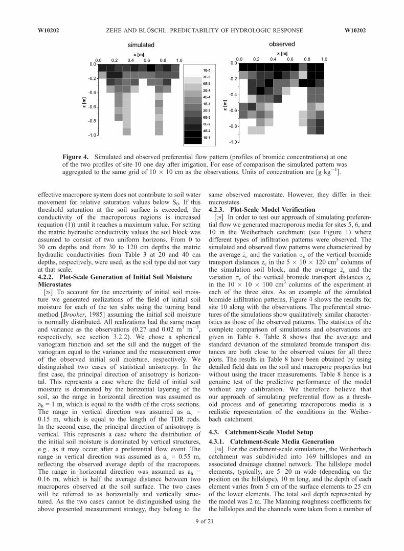
tial flow we generated macroporous media for sites 5, 6, and10 in the Weiherbach catchment (see Figure 1) wheredifferent types of infiltration patterns were observed. Thesimulated and observed flow patterns were characterized bythe average �zc and the variation sc of the vertical bromidetransport distances zc in the 5 � 10 � 120 cm3 columns ofthe simulation soil block, and the average �zc and thevariation sc of the vertical bromide transport distances zcin the 10 � 10 � 100 cm3 columns of the experiment ateach of the three sites. As an example of the simulatedbromide infiltration patterns, Figure 4 shows the results forsite 10 along with the observations. The preferential struc-tures of the simulations show qualitatively similar character-istics as those of the observed patterns. The statistics of thecomplete comparison of simulations and observations aregiven in Table 8. Table 8 shows that the average andstandard deviation of the simulated bromide transport dis-tances are both close to the observed values for all threeplots. The results in Table 8 have been obtained by usingdetailed field data on the soil and macropore properties butwithout using the tracer measurements. Table 8 hence is agenuine test of the predictive performance of the modelwithout any calibration. We therefore believe thatour approach of simulating preferential flow as a thresh-old process and of generating macroporous media is arealistic representation of the conditions in the Weiher-bach catchment.

4.3. Catchment-Scale Model Setup

4.3.1. Catchment-Scale Media Generation[30] For the catchment-scale simulations, the Weiherbach

catchment was subdivided into 169 hillslopes and anassociated drainage channel network. The hillslope modelelements, typically, are 5–20 m wide (depending on theposition on the hillslope), 10 m long, and the depth of eachelement varies from 5 cm of the surface elements to 25 cmof the lower elements. The total soil depth represented bythe model was 2 m. The Manning roughness coefficients forthe hillslopes and the channels were taken from a number of

Figure 4. Simulated and observed preferential flow pattern (profiles of bromide concentrations) at oneof the two profiles of site 10 one day after irrigation. For ease of comparison the simulated pattern wasaggregated to the same grid of 10 � 10 cm as the observations. Units of concentration are [g kg�1].


9 of 21

W10202

irrigation experiments performed in the catchment, as wellas from the literature [see Zehe et al., 2001]. For thehillslopes the following boundary conditions were chosen:free drainage at the bottom, mixed boundary conditions atthe interface to the stream, atmospheric pressure at theupper boundary, no flux boundary at the watershed bound-ary. Because of the spatially highly organized hillslope soilcatena observed in the Weiherbach catchment, all hillslopesin the model catchment were given the same relative catenawith Calcaric Regosol in the upper 80% and Colluvisolin the lower 20% of the hill. The corresponding vanGenuchten-Mualem parameters are listed in Table 5.[31] The measurements of macroporosity at 15 sites in the

Weiherbach catchment suggested high values in the moistColluvisols at the hill foot and low values at the top andmiddle slope sectors (section 3.3.2). On the foot of thehillslopes the macropore volumes typically were 1.5 �10�3 m3 for 1 m2 sampling area while on the top theytypically were 0.6 � 10�3 m3 [Zehe, 1999, Figure 4.1]. Themost parsimonious approach that accounts for this struc-tured variability is a deterministic pattern of the macro-porosity factor with scaled values of the macroporosityfactor at each hillslope. We chose the macroporosity factorto 0.6fm at the upper 70% of the hillslope, 1.1fm at the midsector ranging from 70 to 85% of the hillslope, and 1.5fm atthe lowest 85 to 100% of the slope length, where fm is theaverage macroporosity factor of the hillslopes. The depth ofthe macroporous layer was assumed to be constant through-out the whole catchment and was set to 0.5 m. The onlyremaining free parameter is the average macroporosityfactor fm of the hillslopes. As the number of macroporesconnected to the soil surface varies throughout the year, thefm value has to be calibrated when we focus on the eventscale. Within each model element we assumed that fmrepresents all the subgrid variability of preferential flow ina lumped way, so we did not include the small-scalevariations of bulk hydraulic conductivity due to individualmacropores of the plot-scale set up.4.3.2. Catchment-Scale Generation of Initial SoilMoisture Microstates[32] To generate the initial soil moisture patterns at the

catchment scale we used a combination of two-dimensionalturning band simulations (TB) and simple updating (SUK).The TB algorithm [Brooker, 1985] was used to generateunconditional fields with the observed average, variance

and range given in Table 6 assuming that soil moisture isnormally distributed. To condition the TB generated fieldsto the soil moisture observations we resampled the field atthe measurement locations and computed the differences(i.e., the residuals dq) between observed and generated soilmoisture. We interpolated the residuals using SUK andadded them to the unconditional field, which produced aconditional field of initial soil moisture that gave exactly theobserved soil moisture values at the measurement locations.SUK [Bardossy et al., 1996] is a geostatistical interpolationmethod that makes use of proxy information that is knownat a higher spatial resolution than the variable of interest. Itis based on a relationship between the variable of interestand a proxy variable (L) through a conditional mean mL andvariance VarL. The soil moisture residual dq at an arbitrarylocation is estimated as a sum of the Ordinary Krigingestimator and an estimator based on mL plus a zero meanerror eL with variance VarL:

dq xð Þ ¼ l0 mL xð Þ þ eL xð Þ� �

|fflfflfflfflfflfflfflfflfflfflfflfflffl{zfflfflfflfflfflfflfflfflfflfflfflfflffl}proxy information

þXNi¼1

lidq xið Þ|fflfflfflfflfflfflfflffl{zfflfflfflfflfflfflfflffl}

Kriging estimator measurementsð Þ

ð4Þ

For assisting in the interpolation on the catchment scale weexamined two proxy variables. One proxy variable was thetopographical index of Beven and Kirkby [1979], calculatedfrom the digital elevation model at a 12.5 m resolution. Theother proxy variable was the residual soil water content. It isdefined here as the water content at a suction equal to thepermanent wilting point, and is a measure of the amount offine pores in the soil. It was estimated from the soil map at a50 m resolution. For the two rainfall events, Table 6 lists theaverage, variance and range of the observed spatialdistribution of measured soil moisture, as well as thecoefficient of determination R2 from a linear regression ofsoil moisture and the two proxies. The residual water contentwas the more consistent predictor of soil moisture for the twoevents although the coefficients of determination are small.We therefore used residual water content as a proxy variablein the interpolation of the soil moisture residuals to conditionthe TB generated fields. Within each model element weassumed that the soil moisture so estimated is a representativevalue over the entire element, so we did not include the small-scale variations of soil moisture of the plot-scale set up.4.3.3. Catchment-Scale Model Calibration andVerification[33] We calibrated the catchment-scale model by adjust-

ing the macroporosity factor. We estimated the initial soilmoisture patterns by interpolating the observations usingSUK interpolation in a similar way as equation (4), but qwas interpolated rather than dq. For rainfall event 1, whichoccurred in June 1994, we found an optimum macroporosityfactor of fm = 2.1. The simulated hydrographs for fm valuesranging from 0 to 3 are shown in Figure 5 (top) along withthe calibration result. Zehe et al. [2001] used the same valueof fm = 2.1 in long term simulations of the completehydrologic cycle of the Weiherbach catchment which pro-duced unbiased runoff simulations. The rainfall events 1(June 1994) and 2 (August 1995) are very similar in termsof their magnitudes, average intensities (Table 4) and initialsoil moistures. However, the corresponding event runoffcoefficients calculated from the observed hydrographs differ

Table 8. Test of the Plot-Scale Model: Average zc and Standard

Deviation sc of the Bromide Transport Distance for the Simulated

and Observed Flow Patternsa

Site q, m3 m�3Infiltration

TypeFlowPattern �zc , m sc, m

10 0.27 preferential observed 0.173 ± 0.025 0.071 ± 0.00110 0.27 preferential simulated 0.152 ± 0.019 0.058 ± 0.0106 0.25 intermediate observed 0.109 ± 0.006 0.040 ± 0.0016 0.25 intermediate simulated 0.098 ± 0.015 0.035 ± 0.0085 0.23 matrix flow observed 0.063 ± 0.003 0.013 ± 0.0015 0.23 matrix flow simulated 0.083 ± 0.027 0.048 ± 0.024

aIn the case of the simulations, plus/minus values are the standarddeviations of �zc and sc between realizations. In the case of the observations,plus/minus values have been calculated from the measurement errors byerror propagation. q [m3 m�3] is the initial soil moisture. The correspondingobserved flow patterns are given in Figures 2 and 3.

10 of 21


by a factor of almost 2 (Table 4). Apparently, the infiltrationcapacity of the soil was higher in August 1995 than it was inJune 1994. This difference is likely related to a seasonalvariation of the number of macropores (i.e., earthwormburrows) that are connected to the soil surface. Thisinterpretation is consistent with the findings of severalauthors discussed in a review of Flury [1996, pp. 34–36]on transport of pesticides in the soil. Flury notes thatcontinuous macropores are disrupted by plowing e.g., inspring and reconnected to the soil surface by earthwormactivity during summer. For an accurate simulation ofevent 2 we had to increase the fm value to 3.2 (Figure 5,bottom). As we allowed some degree of calibration for bothevents (Figure 5), the comparison cannot be considered afull verification. However, we only adjusted a single pa-rameter (fm) and the shape of the simulated hydrographs isvery close to the observed hydrographs for both events. Wetherefore believe that the model is a realistic representationof the runoff processes in the Weiherbach catchment withthe caveat that fm is difficult to estimate a priori. As thefocus of the further simulations was on event 2, we used anaverage fm value of 3.2.

5. Monte Carlo Simulation Results

5.1. Simulated Plot-Scale Tracer Experiments

[34] For the plot-scale simulation study we generatedthree media of 1 � 1 � 1.2 m3 in size, one with a macro-porosity factor as observed during the field experiment at site10 (termed plot A), one with a macroporosity factor that wasone tenth of the observed value at site 10 (termed plot B),and one without macroporosity (fm = 0) (termed plot C).We varied the average initial soil moisture from 0.14 to0.38 m3 m�3 in steps of 0.01 m3 m�3 to examine its effecton the predictability of hydrologic response. We assumed a

standard deviation of 0.02 m3m�3 which is the observedvalue (see section 3.2.2). For each of these cases wegenerated 40 realizations of soil moisture patterns by theTurning Band method. The irrigation depth and the bromideconcentration in all simulations were set to IC = 25.3 mm andC = 0.165 g L�1, respectively, which are the same values asin the field experiment. The irrigation was simulated at2 different average intensities, at 11 mm h�1 which is thesame value as in the field experiment and at 2.2 mm h�1.The irrigation was represented by constant intensity rainfallover 2.3 h and 11.5 h for the two average intensities to keeprainfall depth the same. As all the soil profiles in the fieldwere excavated one day after the onset of irrigation, thesimulation time was one day in all cases.[35] To characterize each simulated tracer pattern we

computed the average �zc and the standard deviation sc ofthe vertical bromide transport distances for the simulatedpattern, as these parameters have been useful in identifyingthe presence of preferential flow in the observed patterns(compare Figure 3 and section 3.3). To characterize theensemble of simulated tracer patterns, we calculated thecoefficient of variation Cv and the scaled range ns ofthe average bromide transport distance �zc

i within all Ntrial =40 trials (i.e., realizations) of a given average initial soilmoisture:

zc ¼1

Ntrial

XNtrial

i¼1

zic; fc ¼

ffiffiffiffiffiffiffiffiffiffiffiffiffiffiffiffiffiffiffiffiffiffiffiffiffiffiffiffiffiffiffiffiffiffiffiffiffiffiffiffiffiffiffiffiffiffiffi1

Ntrial � 1

XNtrial

i¼1

zic � zc� �2

vuut

Cv ¼fc

zc

ns ¼max zic

� ��min zic

� �zc

ð5Þ

Figure 5. (top) Simulated discharges (thin solid lines) for event 1 (27 June 1994) for macroporosityfactors ranging from fm = 0 to 3. Increasing values of fm correspond to decreasing runoff. The best fit tothe observed hydrograph is obtained for fm = 2.1 (circles). (bottom) Event 2 (13 August 1995) and best fitsimulation with fm = 3.2. Weiherbach catchment, 3.6 km2 catchment area.


11 of 21

W10202

Cv and ns are used to quantify the effect of uncertain initialsoil moisture on the infiltration response.

5.1.1. Simulations With Observed Macroporosityand I == 11 mm h

�1

[36] Figure 6 (top) shows the coefficient of variation Cv

and the scaled range ns of the average bromide transportdistance �zc within all trials plotted against the average initialsoil moisture �q for the simulated irrigation at the highirrigation rate of I = 11 mm h�1. For initial soil moisturesbelow about 0.19 m3 m�3 and above about 0.28 m3 m�3 thecoefficient of variation Cv and the scaled range ns arerelatively small. This means that the repeated trials of thesimulated irrigation lead to the same type of infiltration, lowaverage bromide transport distances �zc for average initial

moisture values �q below 0.19 m3 m�3, and large �zc valuesfor �q exceeding 0.28 m3 m�3. The uncertainty of the initialsoil moisture pattern expressed as the different possibleinitial microstates hence does not significantly affect thetype of simulated flow pattern. For average initial soilmoistures ranging from 0.19 to 0.28 m3 m�3 the simulationsproduce a completely different behavior. In this range, theuncertainty of the initial state is amplified, leading to acoefficient of variation of up to 0.21 and a scaled range ofup to 0.9. Thus, depending on the microstate of the initialsoil moisture patterns, either fast or slow transport canestablish during the infiltration event, which is reflectedby a large variation of the bromide transport distancesbetween the trials. We call this range of average initial soil

Figure 6. Coefficient of variation Cv and scaled range ns of the average bromide transport distance �zcresulting from differences in the microstate of initial soil moisture plotted against the average initial soilmoisture �q. Simulations at hypothetical plot A for irrigation rates of (top) 11 mm h�1 and (middle)2.2 mm h�1. (bottom) Cv and ns of hypothetical plot C (without macropores). The threshold saturation S0for initiation of macropore flow corresponds to a soil moisture value of 0.32 m3 m�3.

12 of 21


moisture the unstable range because different microstatesthat belong to the same observed macrostate of initial soilmoisture can lead either to attenuated or to enhancedinfiltration relative to the average conditions.5.1.2. Simulations With Observed Macroporosityand Smaller I[37] Figure 6 (middle) shows the coefficient of variation

and the scaled range of �zc within all trials plotted against theaverage initial soil moisture �q for the simulated irrigation ofplot A at a low irrigation intensity of I = 2.2 mm h�1. Theresults are similar to the previous case but the coefficient ofvariation and the scaled range in the unstable range of initialsoil moisture (0.19 to 0.28 m3 m�3) increase to values of0.35 and 1.2, respectively. This means that reducing theintensity enhances the dependence of the simulated flowpatterns on the microstate of the initial soil moisture. Theminimum average bromide transport distance calculated inthe repeated trials for an average initial soil moisture of0.22 m3 m�3 is only one third of the maximum value. Thiswide spreading of the average bromide transport distancesindicates that the expected type of infiltration can be fast,slow or a combination thereof. For average initial soilmoisture values below 0.19 m3 m�3 and above 0.28 m3

m�3 the infiltration type is stable and repeated trials lead toa low variation of the average bromide transport distance.[38] To examine the flow regime of the tracer patterns

resulting from the repeated trials at 0.14, 0.24 and0.38 m3 m�3 average soil moisture in more detail, theaverage bromide transport distance �zc has been plottedagainst the variation of the bromide transport distance scin Figure 7. To interpret the flow regime in Figure 7, theobservations in Figure 3 can be recalled which suggest thatlow values of �zc and sc are associated with matrix flowwhile large values of �zc and sc are associated with prefer-ential flow. This means that for the small average moisture

values (�q = 0.14 m3 m�3) in Figure 7 matrix flow occurredalone while for the large average moisture values (�q =0.38 m3 m�3) preferential flow occurred in all cases. Incontrast, the parameters associated with �q = 0.24 m3 m�3

(circles in Figure 7) cover nearly the whole range between thetwo extreme ends of the spectrum of infiltration regimes. Ifwe adopt the classification of flow patterns into matrix flowdominated, intermediate, preferential and strongly preferen-tial for �zc values ranging from 0.04–0.07, 0.07–0.10, 0.10–0.13 and 0.13–0.17 m from Figure 3 to the simulations, weobtain the following results: For an average initial soilmoisture of 0.24 m3 m�3, the simulated repetition of thetracer experiment leads to matrix flow patterns in 39%,intermediate flow patterns in 38%, preferential flow patternsin 20% and strongly preferential flow patterns in 2% of thetrials. Any type of flow pattern seems to be possible with afinite probability, so the observed macrostate of initial soilmoisture may not be related to a unique type of flow regime.In the stable ranges, the knowledge of themacrostate of initialsoil moisture is sufficient to predict the type of flow pattern.In the unstable range, however, this is not the case.[39] Table 9 gives the maximum and minimum values of

average bromide transport distance �zc at the average initialsoil moisture value of maximum uncertainty as well as thespatial correlation between the corresponding realization ofthe initial soil moisture pattern and the bulk hydraulicconductivity kB of the model soil. Table 9 indicates thatpositive correlations between local saturation and localmacropore-related hydraulic conductivity produce largeaverage transport distances, while negative correlationsproduce much smaller transport distances. The correlationcoefficients are only of the order ±0.3, which are weakcorrelations. This means that at the moisture state where theuncertainties in the microstate translate into the largestuncertainties in hydrologic response, small differences inthe hydrologic conditions can lead to drastic differences inhydrologic response. As can be seen from Table 9, theprincipal direction of anisotropy of the generated initial soilmoisture has only a small influence on the state-dependentuncertainty of the simulated tracer patterns.5.1.3. Simulations With Reduced Macroporosity[40] For comparison, we reduced the macroporosity fac-

tor to one tenth of the observed value and reran thesimulations. Interestingly, this case produced qualitativelyvery similar results to the previous cases. Uncertain initialconditions, again, produced highly uncertain infiltrationpatterns in the unstable range of average moisture betweenabout 0.19 and 0.28 m3 m�3. In the stable range, i.e., forvalues either smaller than 0.19 or larger than 0.28 m3 m�3,the type of the simulated infiltration patterns was stable.However, if the macroporosity factor of the model soil isreduced to zero (Figure 6, bottom) both the coefficient ofvariation and the scaled range get very small. This meansthat, no matter what the initial soil moisture pattern is, theresulting infiltration pattern will always look similar. Thestate-dependent predictability of the simulated plot-scaletracer pattern is therefore a direct consequence of themacroporous heterogeneity and the presence of a thresholdprocess.

5.2. Simulated Catchment Response

[41] To quantify the impact of uncertain initial soilmoisture on flood response at the catchment scale we

Figure 7. Standard deviations sc plotted against theaverages �zc of the simulated vertical bromide transportdistances for average initial soil moisture values of 0.14,0.24, and 0.38 m3 m�3. The bromide centers of mass of theflow patterns in the unstable range (�q = 0.24) cover nearlythe whole spectrum of infiltration regimes from matrix flowdominated to strongly preferential patterns. The irrigationdepth and rate were 25.3 mm and 2.2 mm h�1, respectively(hypothetical plot B).


13 of 21

W10202

simulated the runoff response to rainfall event 2 using 20turning band generated fields of initial soil moisture condi-tioned to the soil moisture observations prior to event 2. Thesill, nugget and range of the generated initial soil moisturepatterns were those in Table 6 (event 2). The spatial mean ofall of these fields was 0.26 m3 m�3 consistent with theobserved soil moisture at the beginning of this event(Table 4). We then added constant values ranging from�0.12 to 0.12 m3 m�3 to each realization in order to obtainfields with average initial soil moisture ranging from0.14 m3 m�3 to 0.38 m3 m�3 in steps of 0.02 m3 m�3,similar to the plot-scale analysis. The different realizationsof the initial soil moisture pattern represent, again, differentpossible microstates consistent with the observed macro-state of initial soil moisture. To investigate the influence ofrainfall intensity we repeated the Monte Carlo simulationsof flood response using a hypothetical rainfall event for

which we reduced the intensity to 50% and scaled time to200%, thus retaining the total rainfall depth. We term thisevent the reduced event 2.5.2.1. Monte Carlo Simulations of Event 2[42] To characterize the ensemble of simulated flood

hydrographs, we calculated the coefficient of variation Cv

and the scaled range ns of the flood peaks Qmax within all20 trials of a given average initial soil moisture in ananalogous way to equation (5). Figure 8 (top) shows thecoefficient of variation Cv and the scaled range ns of Qmax

plotted versus average initial soil moisture. For initial soilmoistures below about 0.18 m3 m�3 and above about0.30 m3 m�3 the coefficient of variation Cv and the scaledrange ns are relatively small. This means that the repeatedtrials of the simulated rainfall events lead to consistentrunoff response, small flood peaks for average initialmoisture values �q below 0.18 m3 m�3, and large floodpeaks for �q exceeding 0.30 m3 m�3. The uncertainty of theinitial soil moisture pattern expressed as the different possi-ble initial microstates hence does not significantly affectflood response for these conditions. For average initial soilmoistures ranging from about 0.18 to 0.30 m3 m�3, however,the uncertainty of the initial state is amplified, leading to acoefficient of variation of up to 0.08 and a scaled rangeof up to 0.32. Thus, for the same observed macrostate ofinitial soil moisture the flood peaks can differ remarkably,depending on the microstate.[43] The shape of the dependence of the coefficient of

variation Cv and the scaled range ns on the averageinitial soil moisture in Figure 8 (top) is similar to thecorresponding values for the plot scale in Figure 6 (topand middle). The soil moisture associated with the maxi-mum uncertainty is 0.24 m3 m�3 which is close to a value of0.22 m3 m�3 found at the plot scale. However, the scaledrange and coefficient of variation computed for Qmax are

Table 9. Minima and Maxima of the Average Bromide Transport

Distance �zc, Average Initial Soil Moisture �q, and Correlation

Coefficient R Between the Initial Soil Moisture Pattern and the

Bulk Hydraulic Conductivity kB for Each Case of Anisotropy for

Simulation Results

�zc, m R �q, m3 m�3 Anisotropy Case

Plot AMinima 0.049 �0.31 0.22 horizontalMaxima 0.135 0.24 0.22 horizontalMinima 0.056 �0.28 0.22 verticalMaxima 0.122 0.26 0.22 vertical

Plot BMinima 0.046 �0.39 0.22 horizontalMaxima 0.122 0.28 0.22 horizontalMinima 0.060 �0.14 0.22 verticalMaxima 0.107 0.21 0.22 vertical

Figure 8. Coefficient of variation Cv and scaled range ns of flood peaks resulting from differences in themicrostate of initial soil moisture plotted against the average initial soil moisture �q. Simulations for theWeiherbach catchment (3.6 km2). (top) Original event 2; (bottom) reduced event 2.

14 of 21


clearly smaller than the corresponding values computed forthe average bromide transport distance �zc. In contrast to theplot scale, the effect of uncertain initial soil moisture on theflood peaks increases as the average initial soil moistureapproaches very small values. This increase is related to thepresence of two soil types in the case of the catchment scale.As can be seen from Figure 9, over most of the soil moisturerange, the unsaturated hydraulic conductivity of the CalcaricRegosol is larger than that of the Colluvisol. In the dry case,infiltration only occurs through matrix flow which will be

different in these two soils. The superposition of differentmicrostates of the initial soil moisture pattern on the soiltype related conductivity pattern will therefore producelarge differences in infiltration and hence runoff generation.[44] To further highlight the dependence of the simulated

hydrographs on the microstate of initial soil moistureFigure 10 shows the simulated catchment response foraverage initial soil moisture values of 0.14 m3 m�3,0.24 m3 m�3 and 0.38 m3 m�3. In the dry case (Figure 10,top left), the runoff response to the first rainfall burst isremarkably large and there is almost no response to thesecond burst 2. This counterintuitive result is due to the soilmoisture being below the threshold for the initiation ofmacropore flow, so no macropore flow takes place at thebeginning of the event. The matrix initial soil hydraulicconductivity associated with the dry soils is also very low(10�13–10�9 m s�1). This conductivity corresponds to arainfall intensity of less than 0.004 mm h�1, which is muchlower than the average precipitation intensity of 22 mm h�1

(Table 4), so most of the rainfall becomes runoff at thebeginning of the first peak. During the second part of theevent, however, the soil wets up and water may infiltrateand not produce runoff. The runoff response in the wet case(Figure 10, bottom right) is quite different with moderateresponse to the first rain burst and large response to thesecond burst. Because of the high initial relative saturation(S = 0.95 in the Colluvisol and 0.86 in the Calcaric Regosol)the initial hydraulic conductivity of the soil is on the order of10�5 m s�1 (including macropore effects). This valuecorresponds to a rainfall intensity of 36 mm h�1 and exceedsthe average rainfall intensity of 22 mm h�1, so the first floodpeak in the wet case is smaller than that in the dry case. Therunoff response in the intermediate case (Figure 10, bottomleft) is lower than in the two extreme cases. This is because,

Figure 9. Characteristic unsaturated hydraulic conductiv-ity curves for the Calcaric Regosol (dashed) and theColluvisol (solid). K is the unsaturated hydraulic conduc-tivity, and q is the soil moisture.

Figure 10. Simulated catchment runoff response (thin lines) to rainfall event 2 for average initial soilmoisture values of (top left) 0.14, (bottom left) 0.24, and (bottom right) 0.38. The thick lines in thebottom left panel represent the largest and smallest simulated flood response in the ensemble ofrealizations. The dashed lines are the observed hydrographs. (top right) Hyetograph of event 2.Weiherbach catchment, 3.6 km2 catchment area.


15 of 21

W10202

in this case, the hydraulic conductivity is large enough for alarge part of rainfall to infiltrate, and the soil is dry enough tostore water and not produce saturation excess runoff.[45] The hydrographs for low average initial moisture

show some dependence on the microstate of the initialsoil moisture patterns, those for the high average initialmoisture show almost no dependence (Figure 10). Incontrast, the simulated hydrographs for the intermediateaverage initial soil moisture of 0.24 m3 m�3 exhibit asignificant dependence on the soil moisture microstate.The difference between the two enveloping hydrographsis on the order of 1 m3 s�1 over more than an hour (t = 160–

161 h) which is large as compared to an observed peak ofless than 3 m3 s�1. These results are consistent with thepeak in sensitivity of ns = 0.32 in Figure 8.[46] To better understand the differences in the runoff

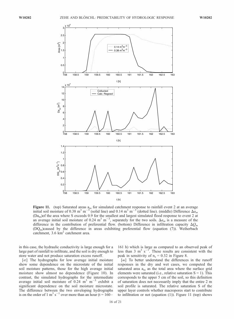
responses in the dry and wet cases, we computed thesaturated area ass as the total area where the surface gridelements were saturated (i.e., relative saturation S = 1). Thiscorresponds to the upper 5 cm of the soil, so this definitionof saturation does not necessarily imply that the entire 2 msoil profile is saturated. The relative saturation S of theupper layer controls whether macropores start to contributeto infiltration or not (equation (1)). Figure 11 (top) shows

Figure 11. (top) Saturated areas ass for simulated catchment response to rainfall event 2 at an averageinitial soil moisture of 0.38 m3 m�3 (solid line) and 0.14 m3 m�3 (dotted line). (middle) Difference Dam(Dam)of the area where S exceeds 0.9 for the smallest and largest simulated flood response to event 2 atan average initial soil moisture of 0.24 m3 m�3, separately for the two soils. Dam is a measure of thedifference in the contribution of preferential flow. (bottom) Difference in infiltration capacity DQm

(DQm)caused by the difference in areas exhibiting preferential flow (equation (7)). Weiherbachcatchment, 3.6 km2 catchment area.

16 of 21


the time series of ass for the dry and wet cases of Figure 10.In the dry case, ass increases less steep and at a later time thanin the wet case, but toward the end of the event it remains at alarger value for a longer time. This is because the soils arenot as readily drained as in the wet case since the lowerlayers are drier. We now intend to explain the differencebetween the two enveloping hydrographs simulated for theintermediate average soil moisture conditions (i.e., thicklines in Figure 10, bottom left). For the lower and upperenveloping hydrographs the total areas where soil watersaturation in the upper 5 cm exceeded a value of 0.9 werecomputed and denoted as am

l and amu , respectively. In each

case, this is the total area in the catchment where strongpreferential flow may take place according to equation (1).We then calculated the difference of these two areas:

am tð Þ � ajS > 0:9f g

Dam tð Þ ¼ alm � aum

ð6Þ

This was done for each soil type separately. The results arethe Dam curves shown in the Figure 11 (middle). Thesecurves represent the difference in the total area wherepreferential flow takes place. As expected, the differencesare always positive which means that the total area wherepreferential flow takes place is always larger for the lowerflood envelope than for the upper flood envelope. Becauseof the larger area where preferential flow is initiated, morewater can infiltrate. To obtain a quantitative estimate of thedifference between the infiltrating water in the two cases wemultiplied Dam by the hydraulic conductivity and thecorresponding macroporosity factors (see definition inequation (1)).

DQm tð Þ ¼ Dam tð Þk qð ÞfmS � S0

1� S0ð7Þ

This was done for each soil type separately. The sum of theresulting DQm values of the two soils is shown in Figure 11(bottom). Figure 11 (middle) indicates that the difference ofthe total infiltrating water is on the order of 1 m3 s�1, whichis consistent with the difference of the two envelopinghydrographs in Figure 10 (bottom left). This corroboratesour interpretation that the differences in the simulated floodresponses stem from the differences in the total areas thatexhibit preferential flow in the catchment.5.2.2. Simulations With Reduced PrecipitationIntensity[47] For the case of reduced precipitation intensities

(reduced event 2) Figure 8 (bottom) shows the coefficientof variation Cv and the scaled range ns of the flood peaksQmax that result from the uncertainties in the microstate ofsoil moisture, plotted versus average initial soil moisture.The simulations yield similar result as the correspondingsimulations of the original rainfall event 2 (Figure 8, top)but the uncertainty increases. For the intermediate averageinitial soil moisture range the coefficient of variation and thescaled range give maxima of about 0.15 and 0.42, respec-tively. In contrast to the original event 2, the dependence onthe microstate of the initial soil moisture increases stronglyas soil moisture approaches dry conditions and the maxi-mum coefficient of variation and the scaled range for drysoils are 0.25 and 1.1, respectively. It appears that, as therainfall forcing decreases in intensity, the role of the

nonlinearity increases. At the dry end of soil moisture theuncertainty is particularly high. This again, is related tocontrasting soil hydraulic characteristics of the two soils inthe catchment (see Figure 9).

6. Discussion and Conclusions

6.1. State Dependence of Predictability

[48] We have examined the effect of uncertainty in themicrostate of initial soil moisture on the predictability ofhydrologic response at the plot and catchment scales. TheMonte Carlo analyses indicate that considerable uncertaintydoes exist at both scales, so the predictability is indeedlimited by the availability of only a finite number ofmeasurements to specify the macrostates of initial soilmoisture. This is consistent with the qualitative assessmentof Grayson et al. [1995] and Merz and Bardossy [1998] andothers that different spatial patterns of initial soil moisturecan produce vastly different results of runoff response evenif the spatial statistical distributions are the same. At the plotscale, the processes may switch between matrix and pref-erential flow, and at the catchment-scale processes mayswitch between runoff generation mechanisms and thesetransitions, under some conditions, cannot be captured bythe measurements. The uncertainty in hydrologic response,again depending on the conditions and the variable exam-ined, may range up to a coefficient of variation of 0.4 and ascaled range of the uncertainty of 1 implying a maximumabsolute error of 100%.[49] The simulations indicate that the predictability of the

hydrologic response depends on the average initial state ofsoil moisture. At both the plot and catchment scales thereexists an unstable range where the predictability of hydro-logic response is poor, and a stable range where thepredictability is significantly better. The unstable rangeranges from an average soil moisture of about 0.18 to0.30 m3m�3 at both scales and the uncertainty peaks around0.22 m3 m�3 (Figure 6, top, and Figure 8, top). For dryconditions (average initial soil moisture below 0.18 m3 m�3)and for wet conditions (average initial soil moisture above0.30 m3 m�3) the predictability is much better, so this is thestable range. Clearly, this state-dependent predictability isrelated to the presence of threshold processes. If the systemis close to the threshold the predictability is poor. The mainthreshold in the Weiherbach catchment is the transition frommatrix to macropore flow. We conceptualized this transitionby a threshold value of relative saturation for the initiationof macropore flow which we set to S0 = 0.8. This value isequivalent to a soil moisture of about 0.32 for the Weiher-bach soils. The unstable range is below this threshold andthis is because the initiation of macropore flow relevant tohydrologic response occurs during the event when the soilmoisture has increased beyond that of the initial conditions.For different event rainfall depths the location of theunstable range will likely change from that in the simula-tions of this event. Also, in different environments withdifferent soils the threshold value will be different from thatin the Weiherbach catchment. It is important to note thatstorm runoff generation in the Weiherbach is by infiltrationexcess and there are essentially no subsurface lateral flows.In other catchments, saturation excess and/or subsurfacestorm flow may be the more important contributions to


17 of 21

W10202

storm runoff. Although the detailed characteristics will bedifferent there is evidence that saturation excess runoff,for example, operates as a threshold process [e.g., Westernand Grayson, 1998]. As the type of nonlinear behavior ofa threshold process occurs in many environments and inmany different processes one would expect this state-dependent predictability, albeit at different soil moisturestates, to occur more universally.[50] Representing the macrostate of initial soil moisture

by the distribution function rather than by spatial patternsdoes not account for the small-scale details of the micro-state. One of the important pieces of information that is lostis the correlation between local saturation and local macro-pore-related hydraulic conductivity. At the plot scale, if thesoil was prone to switch from matrix to macropore flow, soilmoisture microstates that were positively correlated with thebulk hydraulic conductivity yielded fast infiltration andtransport associated with preferential flow. This positivecorrelation of some of the microstates stems from thesuperposition of the soil moisture microstates on the timeinvariant pattern of macroporosity. Other microstatesexhibited negative correlations and these produced slowinfiltration and transport associated with matrix flow(Table 9). The correlation becomes important because ofthe nonlinearity introduced by the threshold process. For alinear system one would expect the effects of the correla-tions to average out to a large degree. It was not possible toobtain estimates of this correlation from the field data as thesoil moisture measurements and the mapping of the macro-pore system had to be done at separate plots because of thedisturbance of the soil by each of these measurements. It istherefore not possible to include them in the description ofthe macrostate. Experimental findings of Villholth et al.[1998] and Zehe and Fluhler [2001b] suggest that highvalues of initial saturation in macroporous subregions favorthe occurrence of macropore flow, so positive correlationsprobably occur quite frequently. A similar effect occurs atthe catchment scale. If the soil is prone to switch frommatrix to macropore flow, microstates where, locally, soilmoisture is large at a location of large macroporosities willproduce much larger infiltration rates than if low soilmoisture is colocated with large macroporosities. The timeinvariant patterns of macroporosity are associated with thehillslope soil catena and there is also the effect of thepatterns of matric conductivity associated with different soiltypes. Figure 11 suggests that the uncertainty in floodresponse for the intermediate, unstable, initial soil moistureconditions is mainly due to differences in the total areas thatexhibit preferential flow between different microstates.

6.2. Other Factors Controlling Predictability

[51] There are a number of other factors, in addition to theaverage initial moisture state, that control the effect ofuncertainty in the microstate of initial soil moisture on thepredictability of hydrologic response. The factors examinedin this paper include rainfall intensity, macroporosity andscale.[52] If we reduce the irrigation intensity at the plot scale

from 11 to 2.2 mm h�1 the coefficient of variation betweenthe realizations increases from 0.21 to 0.35 and the scaledrange increases from 0.9 to 1.2 (Figure 6). If we reducethe average rainfall intensity at the catchment scale from

23 mm h�1 to 11.5 mm h�1 the coefficient of variationincreases from 0.08 to 0.25 and the scaled range increasesfrom 0.32 to 1.1 (Figure 8). This means that the predict-ability decreases with decreasing rainfall intensity at bothscales. It appears that, as the rainfall forcing decreases inintensity, the role of the nonlinearity increases. This isbecause lower rainfall intensities are closer to a thresholdwhere surface runoff may or may not be generated whilelarge rainfall intensities will always produce surface runoff. Itshould be noted that the measure for predictability used hereis a relative measure, i.e., the short bromide travel distancesand the small flood peaks associated with the small intensi-ties are relatively more uncertain than larger distances andlarger flood peaks. When reducing rainfall intensities there isalso a shift of the unstable range toward lower average initialsoil moistures at the plot scale, and an additional unstablerange emerges at low average initial soil moistures at thecatchment scale. This, again, is related to the larger sensitiv-ity of runoff response to uncertain initial conditions whenrainfall intensity decreases. In the case of the catchmentscale, the spatial pattern in matric hydraulic conductivitiesrelated to different soils types appears to produce thisadditional sensitivity at the dry end of initial conditions.[53] It is interesting that the value of the macroporosity

does not change the predictability. Plot-scale simulationsperformed with macroporosities of one tenth of the observedvalue produced very similar predictabilities as those with theobserved values. This is because the main uncertainty isintroduced by the transition between matrix and macroporeflow rather than by the flow rate once the macropores havebeen activated. This is a reflection of the importance of thenonlinearity. However, if only matrix flow is allowed theuncertainty decreases vastly. A hydrologic system withonly matrix flow is much more predictable than a systemwhere a transition between matrix and macropore flow maytake place.[54] As simulations at the 1m2 plot scale and the 3.6 km2

catchment scale have been performed in this paper we candraw conclusions on the scale dependence of predictability.The response at the plot scale is measured by an analysis ofthe vertical bromide transport distances of hypotheticalirrigation experiments and the response at the catchmentscale is measured by an analysis of the flood peak dischargeof hypothetical rainfall events, so they are not strictlycomparable. However, because of the similarity of flowand transport scales of motion we believe that generalremarks on the relative orders of magnitude of the predict-abilities are in place. As we go up in scale in the standardcases examined here, the coefficient of variation betweenthe realizations decreases from 0.21 to 0.08 and the scaledrange decreases from 0.9 to 0.32 (Figure 6, top, andFigure 8, top). This means that the predictability increaseswith scale with maximum absolute errors of 90% and 32%at the plot scale and the catchment scale, respectively. Thereare a number of considerations in interpreting this scaledependence. As one goes up in scale one would at least partof the variability expect to average out [see, e.g., Bloschl,1999]. In the catchment-scale model, subgrid variability hasbeen dealt with in a lumped way. Unlike at the plot scalewhere small-scale heterogeneities resulting from individualmacropores were represented in the model, only a singleeffective value of the macroporosity factor fm has been used

18 of 21


in each element of the catchment model. Because of this,one would not expect this small-scale variability to affectcatchment-scale response. This is plausible if we adopt areasoning along the lines of the central limit theorem whereaggregation, in general, produces more linear and lessvariable response [e.g., Sivapalan and Wood, 1986]. Thereduced uncertainty may be partly due to less nonlinearbehavior at the catchment scale. The central limit theorem,however, applies to independent and identically distributedrandom variables. Very likely, the underlying soil variabilityand runoff processes are neither independent nor random,and structured heterogeneity and structured processes maydominate the system response [Bloschl and Sivapalan,1995; Western et al., 2001]. The analyses did indicate astate-dependent predictability at the catchment scale similarto that at the plot scale (Figure 8) and the role of thetransition between matrix and macropore flow is quiteapparent at the catchment scale when examining contribut-ing areas (Figure 11). Part of this threshold effect at thecatchment scale is related to the presence of two differentsoils with contrasting hydraulic characteristics. Differentmicrostates of initial soil moisture may therefore producesignificantly different initial soil hydraulic conductivitypatterns which determine the amount of infiltration excessrunoff that is generated. These analyses suggest that, as onemoves from the plot to the catchment scale, part of thesmall-scale variability averages out but there is also anemerging source of uncertainty that is not present at the plotscale. This idea of variability averaging out and additionalsources of variability becoming important when moving upin scale is consistent with the more general discussion ofvarious hydrologic processes of Western et al. [2003,p.135].[55] We believe there is an additional, and perhaps more

straightforward, interpretation of the increasing predictabil-ity with scale found in this paper. The specifications of themacrostates at the plot and catchment scales in this paperare not exactly the same. At the plot scale we specified themacrostate of initial soil moisture by the first two momentsof the spatial distribution derived from TDR point measure-ments. At the catchment scale the description of the soilmoisture macrostate is more detailed than that at the plotscale as, in addition to the univariate moments, the values atindividual points (through conditioning of the soil moisturerealizations) and the variogram are specified. It is possiblethat the decrease in uncertainty with increasing scale isrelated to using more detailed information at the largerscale. We have argued that this is a typical setup in aresearch catchment as, at the plot scale, disturbances of thesoil by the measurements are more problematic than at thecatchment scale. As we go up in scale, often, more data willbe available which may decrease the uncertainty and henceincrease the predictability. It would be interesting to repeatthe catchment-scale analyses of this paper and specify thefirst and second univariate moments only to examinewhether the level of detail of the macrostate descriptionsaffects the predictability.

6.3. Implications for Process Studies and Modeling

[56] In this study we have put a lot of effort in realisticallyportraying the processes in the Weiherbach catchment in theCATFLOW model by using fairly detailed measurements at

various scales. This gives us some confidence that themodel does reflect the important infiltration and runoffprocesses at both the plot and catchment scales in a realisticway. We therefore can interpret the realizations of the MonteCarlo simulations as repeated plot-scale and catchment-scale experiments. All of these repeated experiments areidentical in their macrostate of initial soil moisture asdefined by what we can typically measure in a researchcatchment but they differ in their microstate of fine-scalesoil moisture variability not captured by the monitoringnetwork. As all these microstates belong to the samemacrostate of initial soil moisture they may not be distin-guished by the measurement strategy used in the field. Thesimulations have indicated that the response will indeed notbe unique if the average initial state approaches a threshold,i.e., if nonlinearity becomes important for the systemresponse. As a consequence, for apparently identical exper-imental conditions preferential flow may or may not occur,solute transport depths can vary by more than 90% andflood peaks can vary by more than 30%. These limits topredictability provide a suitable explanation for apparentlyinconsistent experimental results such as the tracer break-through velocities of Lischeid et al. [2000] that variedbetween 30.6 and 10.6 m d�1 for identical experimentalconditions. By the same token, observed runoff response atthe catchment scale is often difficult to interpret in a uniqueway. We believe, again, that part of this difficulty stemsfrom the intrinsic limits to predictability given a typical setof measurements. Of course, the additional difficulty at thecatchment scale is that the rainfall forcing can not usually becontrolled.[57] One would generally hope that a detailed set of

field measurements would constrain the system stateenough to give unique results when used for hydrologicmodeling but the results of this paper suggest that this isnot necessarily the case. These limits to obtaining uniquerelationships in experiments and observations have directimplications for model representations. Beven [2000,p. 211] notes that ‘‘field process studies are by their natureunique in both space and time; they cannot be repeated underexactly the same boundary and initial conditions,’’ and hegoes on to discuss the implications for modeling. One of theimplications is the need to resort to calibration strategies tomake models work and this is true at various scales [Beven,1989; Grayson et al., 1992]. It is clear that if one calibratesparameters to compensate for the real uncertainty in themicrostate of initial conditions this is likely a ‘‘quick fix’’which may jeopardize the realism of the model. Obviously, amuch better strategy would be to allow for the uncertainty inthe initial microstate rather than to seek a best fit of themodel to the one realization of hydrologic response avail-able. The soil moisture data used in this paper have beenfairly detailed (50 and 61 measurement points at the plot andcatchment scales, respectively). With a few exceptions [e.g.,Western and Grayson, 1998] the number of monitoring siteswill be much lower in most hydrologic studies. This meansthat the predictability will be lower than what has beenobtained in this paper. Also, we considered a single source ofuncertainty only, i.e., the initial conditions, assuming aperfect representation of the governing processes (in termsof model structure and model parameters) and assumingerrors in the forcing to be small. It is clear that these


19 of 21

W10202

additional sources of uncertainty will degrade the predict-ability beyond the results of this paper.[58] We have adopted the concepts of microstates and

macrostates from statistical mechanics and think these arepowerful concepts to analyze the role of measurements inmodeling or, more generally, in representing reality. Thereis, however, an important distinction between hydrologyand standard statistical mechanics. The latter deal with largeaggregates that can be aggregated by statistical methodswhile hydrology usually deals with what Weinberg [1975]terms intermediate systems that cannot be aggregated easilybecause of their intermediate number of degrees of freedomand their complexity (see the discussion of Dooge [1986]).The manifestation of these two characteristics at the plot andcatchment scales is the nonlinearity of hydrologic systemresponse and the presence of organized, nonrandom vari-ability. In this paper we have used a deterministic numericalmodel to examine the aggregation and error propagationeffects but a more elegant approach would involve ananalytical study of the limits to predictability imposed byuncertain microstates. Because of the characteristics ofintermediate systems this will not be easy.[59] The processes studied here involving a switch

between matrix and macropore regimes and the thresholdnature of infiltration excess runoff generation, are oneparticular subset of threshold processes. We believe that theresults of the limits to predictability are more generallyapplicable to hydrologic nonlinear processes. Similar pat-terns of predictability can probably be expected for otherthreshold processes, or more generally, nonlinear processesin hydrology at various spatial and temporal scales. Oneexample in the Weiherbach catchment is a feedback mecha-nism between physical and biological processes. Earthwormactivity controls the dynamics of subsurface flow processesand hence soil moisture through the generation of macro-pores. Conversely, soil moisture controls the macroporelocation to some degree because of the earthworms’ prefer-ence for wetter parts of the catchment. This feedbackmechanism is likely to produce some very interesting non-linearities. Numerous other feedback mechanisms, nonli-nearities and threshold processes exist in hydrology whichare likely to translate into domains of high and low predict-ability. As NRC [2003, p. 21] noted, among the key unre-solved issues and research challenges in hydrology is‘‘separating the predictable and the unpredictable’’. Thispaper is an initial contribution to identifying the boundariesof predictable and unpredictable domains in one particularsetting and it is hoped that future research will shed morelight on the patterns of predictability in more generic hydro-logic contexts.

[60] Acknowledgments. We would like to thank the German Min-istry of Education and Research for financial support of the Weiherbachproject as well as Erich Plate for his thoughtful guidance of the project.We are grateful to Thomas Maurer for significant contributions to theCATFLOW model. The authors would like to thank the Austrian ScienceFoundation (FWF), project no. P14478-TEC, and the Austrian Academyof Sciences, project HO 18, for financial support. The model and thedata set is freely available for academic use by email request [email protected].

ReferencesBardossy, A., U. Haberlandt, and J. Grimm-Strele (1996), Regional scalesof groundwater quality parameters and their dependence on geology andland use, in Groundwater and Subsurface Remediation, edited by

H. Kobus, B. Barczewski, and H.-P. Koschitzky, pp. 195–204, Springer-Verlag, New York.

Beven, K. (1989), Changing ideas in hydrology—The case of physicallybased models, J. Hydrol., 105, 157–172.

Beven, K. J. (2000), Uniqueness of place and process representations inhydrological modeling, Hydrol. Earth Syst. Sci., 4(2), 203–213.

Beven, K. J., and M. J. Kirkby (1979), A physically-based, variable con-tributing area model of basin hydrology, Hydrol. Sci. Bull., 24, 43–69.

Bloschl, G. (1999), Scaling issues in snow hydrology, Hydrol. Processes,13, 2149–2175.

Bloschl, G., and M. Sivapalan (1995), Scale issues in hydrological model-ling: A review, Hydrol. Processes, 9, 251–290.

Bloschl, G., R. B. Grayson, and M. Sivapalan (1995), On the representativeelementary area (REA) concept and its utility for distributed rainfall-runoff modeling, Hydrol. Processes, 9, 313–330.

Boltzmann, L. (1995), Lectures on Gas Theory, translated from German byStephen G. Brush, reprint, Dover, Mineola, N. Y.

Brooker, I. (1985), Two-dimensional simulation by turning bands, Math.Geol., 17(1), 81–90.

Celia, M. A., and E. T. Bouloutas (1990), A general mass-conservativenumerical solution for the unsaturated flow equation, Water Resour.Res., 26(7), 1483–1496.

Dooge, J. C. I. (1986), Looking for hydrologic laws, Water Resour. Res.,22, 46S–58S.

Flury, M. (1996), Experimental evidence of transport of pesticides throughfield soils—A review, J. Environ. Qual., 25(1), 25–45.

Flury, M., H. Fluhler, J. Leuenberger, and W. A. Jury (1994), Susceptibilityof soils to preferential flow of water: A field study, Water Resour. Res.,30(7), 1945–1954.

Gleick, J. (1993), Chaos, Making a New Science, 352 pp., Abacus, London.Grayson, R. B., and G. Bolschl (Eds.) (2000), Spatial Patterns in Catch-ment Hydrology: Observations and Modelling, 404 pp., Cambridge Univ.Press, New York.

Grayson, R. B., I. D. Moore, and T. A. McMahon (1992), Physically-basedhydrologic modeling: 2. Is the concept realistic?, Water Resour. Res., 28,2659–2666.

Grayson, R. B., G. Bloschl, and I. D. Moore (1995), Distributed parameterhydrologic modelling using vector elevation data: THALES and TAPES-C, in Computer Models of Watershed Hydrology, edited by V. P. Singh,pp. 669–696, Water Resour. Publ., Highlands Ranch, Colo.

Grayson, R. B., A. W. Western, F. H. S. Chiew, and G. Bloschl (1997),Preferred states in spatial soil moisture patterns: Local and non-localcontrols, Water Resour. Res., 33(12), pp. 2897–2908.

Landau, L. D., and E. M. Lifshitz (1999), Statistical Physics, Course The-oretical Phys., vol. 5, Butterworth-Heinemann, Woburn, Mass.

Lennartz, B., J. Michaelsen, W. Wichtmann, and P. Windmoser (1999),Time variance analysis of preferential solute movement at a tile-drainedfield site, Soil Sci. Soc. Am. J., 63, 39–47.

Lischeid, G., H. Lange, and M. Hauhs (2000), Information gain usingsingle tracers under steady state tracer and transient flow conditions:The Gardsjon G1 multiple tracer experiments, in Proceedings of theTram’2000 Conference Tracers and Modelling in Hydrogeology, IAHSPubl., 262, 73–77.

Matheron, G., and G. de Marsily (1980), Is transport in porous media alwaysdiffusive? A counter example, Water Resources Res., 16(5), 901–917.

Maurer, T. (1997), Physikalisch begrundete, zeitkontinuierliche Modellier-ung des Wassertransports in kleinen landlichen Einzugsgebieten, Mitt.Inst. Hydrol. Wasserwirt. 61, Univ. Karlsruhe, Karlsruhe, Germany.

Merz, B., and A. Bardossy (1998), Effects of spatial variability on therainfall runoff process in a small loess catchment, J. Hydrol., 212–213, 304–317.

Mualem, Y. (1976), A new model for predicting the hydraulic conductivityof unsaturated porous media, Water Resour. Res., 12, 513–522.

National Research Council (NRC) (2003), Predictability and Limits-to-Pre-diction in Hydrologic Systems, Natl. Acad. Press, Washington, D. C.

Roth, K., and K. Hammel (1996), Transport of a conservative chemicalthrough an unsaturated two-dimensional miller-similar medium withsteady state flow, Water Resour. Res., 32(6), 1653–1663.

Russo, D., J. Zaidel, and A. Laufer (1994), Stochastic analysis of solutetransport in a partially saturated heterogeneous soil: 1. Numerical experi-ments, Water Resour. Res., 30(3), 769–779.

Schafer, D. (1999), Bodenhydraulische Funktionen eines Kleineinzugsge-biets—Vergleich und Bewertung unterschiedlicher Verfahren, Ph.D. dis-sertation, Inst. of Hydromech., Univ. of Karlsruhe, Karlsruhe, Germany.

Sivakumar, B. (2000), Chaos theory in hydrology important issues andinterpretations, J. Hydrol., 227, 1–20.

20 of 21


Sivapalan, M., and E. F. Wood (1986), Spatial heterogeneity and scale inthe infiltration response of catchments, in Scale Problems in Hydrology,edited by V. K. Gupta. I. Rodrıguez-Iturbe, and E. F. Wood, pp. 81–106,D. Reidel Publ., Norwell, Mass.

Tolman, R. C. (1979), The Principles of Statistical Mechanics, reprint,Dover, Mineola, N. Y.

Tsang, Y. W., C. F. Tsang, F. Hale, and V. B. Dverstorp (1996), Tracertransport in a stochastic continuum model, Water Resour. Res., 32(10),3077–3092.

van Genuchten, M. T. (1980), A closed-form equation for predicting thehydraulic conductivity of unsaturated soils, Soil Sci. Soc. Am. J., 44,892–898.

Villholth, K., K. Jensen, and J. Frederica (1998), Flow and transport pro-cesses in a macroporous subsurface-drained glacial till soil: I. Field in-vestigation, J. Hydrol., 207, 98–120.

Webb, E. K., and M. P. Anderson (1996), Simulation of preferential flow inthree dimensional heterogeneous conductivity fields with realistic inter-nal architecture, Water Resour. Res., 32(3), 533–545.

Weinberg, G. M. (1975), An Introduction to General Systems Thinking, 279pp., John Wiley, Hoboken, N. J.

Western, A. W., and G. Bloschl (1999), On the spatial scaling of soilmoisture, J. Hydrol., 217, 203–224.

Western, A. W., and R. B. Grayson (1998), The Tarrawarra data set: Soilmoisture patterns, soil characteristics, and hydrological flux measure-ments, Water Resour. Res., 34(10), 2765–2768.

Western, A. W., G. Bloschl, and R. B. Grayson (2001), Toward capturinghydrological significant connectivity in spatial patterns, Water Resour.Res., 37(1), 83–97.

Western, A., R. Grayson, and G. Bloschl (2002), Scaling of soil moisture: Ahydrologic perspective, Annu. Rev. Earth Planet. Sci., 30, 149–180.

Western, A. W., R. B. Grayson, G. Bloschl, and D. J. Wilson (2003), Spatialvariability of soil moisture and its implications for scaling, in ScalingMethods in Soil Physics, edited by Y. A. Perchepsky, H. M. Selim, andD. E. Radcliffe, pp. 120–142, CRC Press, Boca Raton, Fla.

Wood, E. F. (1976), An analysis of the effects of parameter uncertaintyin deterministic hydrologic models, Water Resour. Res., 12(5), 925–932.

Wood, E. F., M. Sivapalan, K. Beven, and L. Band (1988), Effects ofspatial variability and scale with implications to hydrologic modeling,J. Hydrol., 102, 29–47.

Zehe, E. (1999), Stofftransport in der ungesattigten Bodenzone aufverschiedenen Skalen, Ph.D. dissertation, Univ. of Karlsruhe, Karlsruhe,Germany.

Zehe, E., and H. Fluhler (2001a), Preferential transport of isoproturon ata plot scale and a field scale tile-drained site, J. Hydrol., 247, 100–115.

Zehe, E., and H. Fluhler (2001b), Slope scale variation of flow patterns insoil profiles, J. Hydrol., 247, 116–132.

Zehe, E., T. Maurer, J. Ihringer, and E. Plate (2001), Modelling water flowand mass transport in a Loess catchment, Phys. Chem. Earth B, 26(7–8),487–507.

Zurmuhl, T., and W. Durner (1996), Modelling transient water flow andsolute transport in a biporous soil, Water Resour. Res., 32(4), 819–829.

��G. Bloschl, Institute of Hydraulics, Hydrology and Water Resources

Management, Vienna University of Technology, A-1040 Vienna, Austria.E. Zehe, Institute of Geoecology, University of Potsdam, 14415

Potsdam, Germany. ([email protected])


21 of 21

W10202

predictability of hydrologic response at the plot and ... · predictability of hydrologic response...

Documents