predator behavior and prey demography in patchy habitats

University of South FloridaScholar Commons

Graduate Theses and Dissertations Graduate School

2008

Predator behavior and prey demography in patchyhabitatsBrian J. HalsteadUniversity of South Florida

Follow this and additional works at: http://scholarcommons.usf.edu/etd

Part of the American Studies Commons

This Dissertation is brought to you for free and open access by the Graduate School at Scholar Commons. It has been accepted for inclusion inGraduate Theses and Dissertations by an authorized administrator of Scholar Commons. For more information, please [email protected].

Scholar Commons CitationHalstead, Brian J., "Predator behavior and prey demography in patchy habitats" (2008). Graduate Theses and Dissertations.http://scholarcommons.usf.edu/etd/276

http://scholarcommons.usf.edu/?utm_source=scholarcommons.usf.edu%2Fetd%2F276&utm_medium=PDF&utm_campaign=PDFCoverPages

http://scholarcommons.usf.edu/?utm_source=scholarcommons.usf.edu%2Fetd%2F276&utm_medium=PDF&utm_campaign=PDFCoverPages

http://scholarcommons.usf.edu?utm_source=scholarcommons.usf.edu%2Fetd%2F276&utm_medium=PDF&utm_campaign=PDFCoverPages

http://scholarcommons.usf.edu/etd?utm_source=scholarcommons.usf.edu%2Fetd%2F276&utm_medium=PDF&utm_campaign=PDFCoverPages

http://scholarcommons.usf.edu/grad?utm_source=scholarcommons.usf.edu%2Fetd%2F276&utm_medium=PDF&utm_campaign=PDFCoverPages

http://scholarcommons.usf.edu/etd?utm_source=scholarcommons.usf.edu%2Fetd%2F276&utm_medium=PDF&utm_campaign=PDFCoverPages

http://network.bepress.com/hgg/discipline/439?utm_source=scholarcommons.usf.edu%2Fetd%2F276&utm_medium=PDF&utm_campaign=PDFCoverPages

mailto:[email protected]

Predator Behavior and Prey Demography in Patchy Habitats

by

Brian J. Halstead

A dissertation submitted in partial fulfillment of the requirements for the degree of

Doctor of Philosophy Department of Biology, Division of Integrative Biology

College of Arts and Sciences University of South Florida

Co-Major Professor: Earl D. Mccoy, Ph.D. Co-Major Professor: Henry R. Mushinsky, Ph.D.

Gary R. Huxel, Ph.D. Gordon Fox, Ph.D.

Date of Approval: March 28, 2008

Keywords: Florida scrub, metapopulation, resource selection, survival, vertebrate

© Copyright 2008, Brian J. Halstead

Dedication

To my late grandfathers, James Halstead, Sr. and Leonard Schartner, who instilled in me

a deep interest ecology and natural history, an appreciation for education and attention to

detail, and the belief that anything worth doing is worth doing well. The greatest honor

this dissertation could receive is their approval.

Acknowledgements

No worthwhile endeavor is ever accomplished alone. I am indebted to my wife, Kelly

Browning, for her help with reviewing manuscripts, supplying help and company in the

field, and inspiring me to keep things in perspective. My parents, Tara and James E.

Halstead, Jr., were always very supportive and caring, and even took time out of their

Florida vacation to help me re-install traps that had been uprooted by Hurricane Charley.

Neal Halstead, my brother and colleague, was a tremendous asset. His help in the field

and input on field and analytical methods were indispensable. My co-advisors, Drs. Earl

McCoy and Henry Mushinsky, and committee members, Drs. Gary Huxel and Gordon

Fox, were adept at providing just the right amount of guidance – their efforts were

essential to the successful completion of my dissertation. The staff at Lake Wales Ridge

State Forest, particularly Anne Malatesta, Dave Butcher, and Dawn Johnson, were very

accommodating and provided logistic support. Margi Baldwin, Dee Caretto, and Dr.

Creighton Trahan provided excellent training in surgical technique and provided support

for surgical materials and methods. Numerous graduate students at the University of

South Florida, including Irmgard Lukanik, Katie Basiotis, Jennifer Rhora, Celina

Bellanceau, Shannon Gonzalez, Joel Johnson, David Karlen, Alison Meyers, Kris

Robbins, Travis Robbins, and Jenny Sneed helped with various aspects of this research.

Many undergraduate assistants were essential for the completion of this dissertation, and

deserve greater recognition than space allows.

i

Table of Contents

List of Tables iii

List of Figures v

Abstract vii

Background and Hypotheses 1

Study System: The Florida Scrub 2

Study Organisms 2

Study Questions and Hypotheses 7

Sympatric Masticophis flagellum and Coluber constrictor Select Vertebrate

Prey at Different Phylogenetic Levels 12

Materials and Methods 14

Study Site 14

Field Methods 15

Analytical Methods 16

Results 23

Diet Composition 23

Diet Selection 25

Niche Breadth and Overlap 26

Discussion 26

ii

Masticophis flagellum (Coachwhip) Positively Selects Florida Scrub Habitat at

Multiple Spatial Scales 47


Study Site 48

Field Methods 50


Results 59

Discussion 62

A Greater Abundance of Snakes Results in Lower Survival Rates of Sceloporus

woodi Populations 90


Study Site 91

Field Methods 92


Results 96

Discussion 97

Conclusion: The Predicted Effects of Snake Predation upon Sceloporus woodi

Populations 109

Literature Cited 123

About the Author End Page

iii

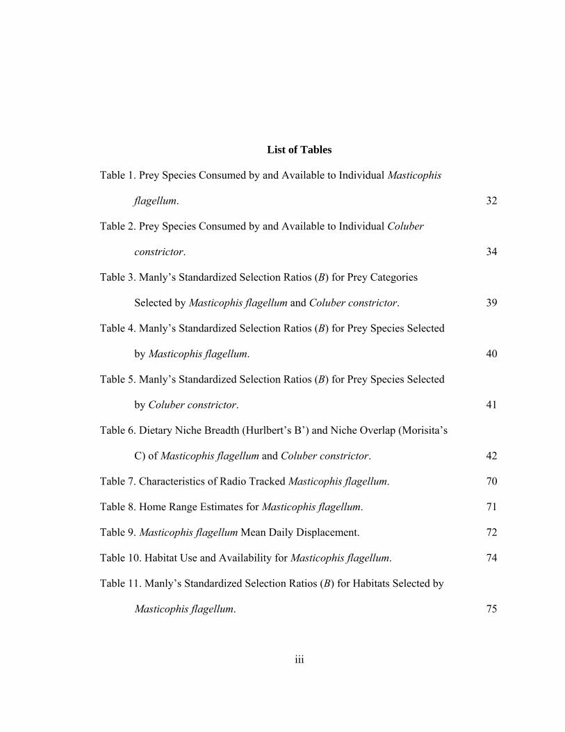
List of Tables

Table 1. Prey Species Consumed by and Available to Individual Masticophis

flagellum. 32

Table 2. Prey Species Consumed by and Available to Individual Coluber

constrictor. 34

Table 3. Manly’s Standardized Selection Ratios (B) for Prey Categories

Selected by Masticophis flagellum and Coluber constrictor. 39

Table 4. Manly’s Standardized Selection Ratios (B) for Prey Species Selected

by Masticophis flagellum. 40

Table 5. Manly’s Standardized Selection Ratios (B) for Prey Species Selected

by Coluber constrictor. 41

Table 6. Dietary Niche Breadth (Hurlbert’s B’) and Niche Overlap (Morisita’s

C) of Masticophis flagellum and Coluber constrictor. 42

Table 7. Characteristics of Radio Tracked Masticophis flagellum. 70

Table 8. Home Range Estimates for Masticophis flagellum. 71

Table 9. Masticophis flagellum Mean Daily Displacement. 72

Table 10. Habitat Use and Availability for Masticophis flagellum. 74

Table 11. Manly’s Standardized Selection Ratios (B) for Habitats Selected by

Masticophis flagellum. 75

iv

Table 12. Summary of Models Evaluated for Habitat Selection by Masticophis

flagellum. 76

Table 13. Florida Scrub Patch Use and Availability for M. flagellum. 77

Table 14. POPAN Jolly-Seber Abundance Estimates for Lizard and

Mammalian Prey in Each Sampled Patch of Florida Scrub. 79

Table 15. Summary of Models Evaluated for Florida Scrub Patch Selection by

Masticophis flagellum. 81

Table 16. Manly’s Standardized Selection Ratios (B) for Florida Scrub Patches

Selected by Masticophis flagellum. 83

Table 17. Home Range Sizes and Movement Distances of Masticophis

flagellum at Different Locations. 84

Table 18. Relative Importance (w+) of Environmental and Individual

Characteristics for Determining the Daily (Re)capture Rate of

Sceloporus woodi. 101

Table 19. Support of Cormack-Jolly-Seber Models for Sceloporus woodi

Populations. 102

Table 20. Relative Importance (w+) of Variables for Determining the Survival

Rate of Sceloporus woodi Populations. 103

v

List of Figures

Figure 1. Occurrence of Prey Categories Consumed by Masticophis flagellum

and Coluber constrictor Expressed as a Proportion of Snakes of Each

Species that Consumed Each Prey Category. 43

Figure 2. Occurrence of Prey Species Consumed by Masticophis flagellum and

Coluber constrictor Expressed as a Proportion of Individuals of Each

Species that Consumed Each Prey Species. 44

Figure 3. Relationship between Prey Category and Predator Size (Snout-vent

Length) for Masticophis flagellum and Coluber constrictor. 45

Figure 4. Ln-transformed Prey Mass as a Function of Ln-transformed Snake

Mass for Masticophis flagellum and Coluber constrictor. 46

Figure 5. Map of the Study Site within the Lake Arbuckle Tract of Lake Wales

Ridge State Forest in Central Florida, USA. 85

Figure 6. Masticophis flagellum Net Squared Displacement Versus Random

Walk Expectations. 86

Figure 7. Masticophis flagellum 100% Minimum Convex Polygon Home

Ranges. 87

Figure 8. Mosaicplot of the Frequency of Behaviors within Habitats. 88

Figure 9. Correspondence Plot of the Association of Snake Behaviors with

Habitats. 89

vi

Figure 10. Map of the Study Site within the Lake Arbuckle Tract of Lake Wales

Ridge State Forest in Central Florida. 104

Figure 11. Schematic Diagram Depicting the Layout of Each Trap Array. 105

Figure 12. Model-averaged Estimates of Abundance for Sceloporus woodi

Populations at Each Trap Array Grouped by Patch Size. 106

Figure 13. Model-averaged Estimates of Recapture Probability for Each

Secondary Period for Sceloporus woodi Populations. 107

Figure 14. Model-averaged Estimates of Survival Rate for Each Primary Period

for Sceloporus woodi Populations. 108

vii

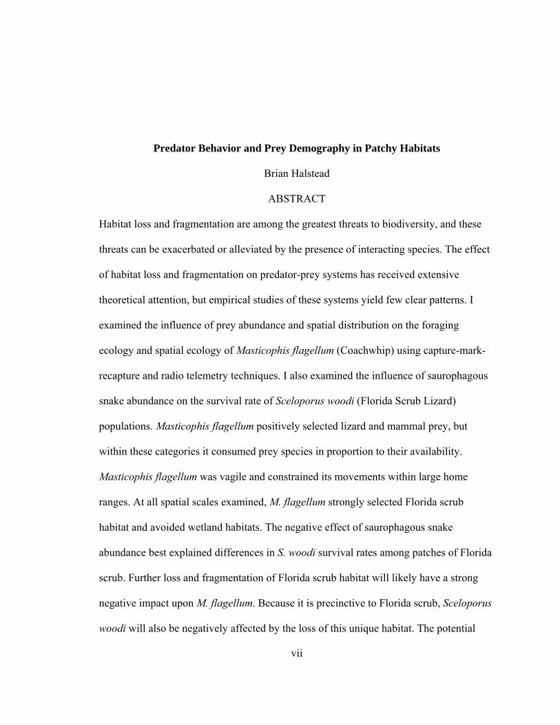
Predator Behavior and Prey Demography in Patchy Habitats

Brian Halstead

ABSTRACT

Habitat loss and fragmentation are among the greatest threats to biodiversity, and these

threats can be exacerbated or alleviated by the presence of interacting species. The effect

of habitat loss and fragmentation on predator-prey systems has received extensive

theoretical attention, but empirical studies of these systems yield few clear patterns. I

examined the influence of prey abundance and spatial distribution on the foraging

ecology and spatial ecology of Masticophis flagellum (Coachwhip) using capture-mark-

recapture and radio telemetry techniques. I also examined the influence of saurophagous

snake abundance on the survival rate of Sceloporus woodi (Florida Scrub Lizard)

populations. Masticophis flagellum positively selected lizard and mammal prey, but

within these categories it consumed prey species in proportion to their availability.

Masticophis flagellum was vagile and constrained its movements within large home

ranges. At all spatial scales examined, M. flagellum strongly selected Florida scrub

habitat and avoided wetland habitats. The negative effect of saurophagous snake

abundance best explained differences in S. woodi survival rates among patches of Florida

scrub. Further loss and fragmentation of Florida scrub habitat will likely have a strong

negative impact upon M. flagellum. Because it is precinctive to Florida scrub, Sceloporus

woodi will also be negatively affected by the loss of this unique habitat. The potential

viii

positive effects of reduced predation pressure from M. flagellum that may accompany

loss and fragmentation of Florida scrub is likely to be offset by increased predation rates

by habitat and dietary generalist predators that incidentally prey upon S. woodi. Despite

the sensitivity of these species to loss and fragmentation of Florida scrub, the prognosis is

good for both M. flagellum and S. woodi on relatively large protected sites containing

xeric habitats managed with prescribed fire.

1

Background and Hypotheses

Habitat loss and fragmentation are among the greatest threats to biodiversity

(Pimm and Raven 2000). The impact of loss and fragmentation of habitat upon

populations can be exacerbated or alleviated by the presence of other interacting species

(Kareiva 1990, Ryall and Fahrig 2006). The effect of habitat loss and fragmentation on

predator-prey systems has received extensive theoretical attention, but empirical studies

of these systems yield few clear patterns (Ryall and Fahrig 2006). Specialist predators

depend upon their prey for positive population growth and are restricted to the same

habitats as their prey. Loss and fragmentation of prey habitat is therefore predicted to be

detrimental to specialist predators, but the effects of specialist predation can increase or

decrease the risk of extinction of prey compared to the effects of habitat loss and

fragmentation alone (Bascompte and Sole 1998, Prakash and de Roos 2002). As dietary

and habitat breadth of the predator increases, negative effects of predation exacerbate the

negative effects of habitat loss and fragmentation and the result is increased extinction

risk of the prey (Swihart et al. 2001, Melian and Bascompte 2002). My goal was to

examine the interaction of a wide-ranging predator with a habitat specialist prey species

occurring in a system of habitat patches, and to evaluate theoretical predictions of the

consequences of this interaction for the persistence of the predator and its prey.

2

STUDY SYSTEM: THE FLORIDA SCRUB

Florida scrub habitat is a unique ecosystem of great conservation importance.

Florida scrub in the interior of peninsular Florida originated as sand dunes in the early

Pleistocene; during the Pliocene, only the very highest of the interior ridges remained

above sea level (Myers 1990). Scrub soils are extremely well-drained, nutrient-poor

sands that support a xerophytic vegetation. Florida scrub is pyrogenic, and fires typically

occur at 10 to 100 year or greater intervals (Myers 1990). The great age and former

isolation as islands has contributed to the occurrence of many organisms precinctive to

Florida scrub, and the Lake Wales Ridge in particular. Forty to sixty percent of the

species found in Florida scrub are precinctive to this habitat (Myers 1990). More than 70

percent of one of the interior ridges, the Lake Wales Ridge, has been lost to agricultural

and residential development over the past fifty years (Myers 1990). Therefore, protection

of existing Florida scrub and ecological data for Florida scrub-precinctive organisms are

high conservation priorities. My study was conducted at the Lake Arbuckle Tract of the

Lake Wales Ridge State Forest (LWRSF), a protected site located on the Lake Wales

Ridge.

STUDY ORGANISMS

Sceloporus woodi is a terrestrial phrynosomatid lizard precinctive to Florida scrub

habitat. Its geographic range is contained entirely within peninsular Florida, and its

occurrence is restricted to Florida scrub habitat in the central ridges of Florida and along

the east and southwest coasts of Florida (Jackson 1973). The limited geographic

3

distribution and habitat specificity of S. woodi contribute to its type 2 rarity (McCoy and

Mushinsky 1992).

Sceloporus woodi is characterized by rapid maturity, low survival rates, and

variable population densities. Sceloporus woodi is sexually mature at 45 mm snout-vent

length at an age of 7-8 months (Hartmann 1993, McCoy et al. 2004). The maximum

recorded lifespan of S. woodi is 27 months, but the average lifespan is only 12.6 months

(McCoy et al. 2004). Mating begins in February and oviposition continues into October

(Jackson and Telford 1974). Mature females can produce three clutches per year, but five

clutches may be possible in favorable years (Jackson and Telford 1974). Hatchlings and

juveniles compose the largest proportion of a population at all times, but the large

proportion of young individuals is especially pronounced in the summer months

(Hartmann 1993, McCoy et al. 2004). Sceloporus woodi densities are highly variable,

ranging from 10.1 individuals/ha (Jackson and Telford 1974) to 124 individuals/ha

(Hartmann 1993, McCoy et al. 2004). Densities are greatest in June with the first

emergence of hatchlings, and decline until the following June (Hartmann 1993, McCoy et

al. 2004). Survival rates of S. woodi are low: only ten percent of juveniles survive to the

end of their first breeding season (McCoy et al. 2004). Mortality of hatchlings and

juveniles is greatest during the summer (Hartmann 1993). Abundance, survivorship, and

recruitment of S. woodi are all positively related to patch size (Hokit and Branch 2003b).

Increased predation may be responsible for observed temporal and spatial differences in

survival rates of S. woodi (Hartmann 1993, Hokit and Branch 2003b, a, McCoy et al.

2004).

4

Although S. woodi can achieve rapid reproduction, it is very limited in its

movements. Home ranges of S. woodi are small, measuring approximately 800 m2 for

males and 400 m2 for females (Hokit et al. 1999). Dispersal of S. woodi is impeded

beyond 200 m, and the maximum dispersal distance is estimated to be 750 m (Hokit et al.

1999). Because of the limited dispersal abilities of S. woodi and the naturally fragmented

nature of Florida scrub, S. woodi exists as metapopulations. Both incidence function and

stage-based models of local dynamics with a dispersal function accurately predict the

occurrence of S. woodi (Hokit et al. 2001). Occurrence of S. woodi in patches of Florida

scrub is positively related to percent bare sand and patch size, the latter likely because of

predation (Hokit et al. 1999). Occurrence is negatively related to patch isolation, and may

be further limited where the habitat matrix consists of dense vegetation (Hokit et al.

1999). The limited dispersal abilities of S. woodi make it particularly susceptible to

anthropogenic habitat fragmentation or alteration (Fahrig and Merriam 1994), and the

exclusion of fire not only eliminates early-successional Florida scrub habitats that are

preferred by S. woodi (Tiebout and Anderson 1997, 2001), but may impede interpatch

dispersal because of increased vegetation density in the matrix surrounding patches of

Florida scrub.

In contrast to the extreme habitat specificity of S. woodi, two of its potential

predators, Coluber constrictor (Eastern Racer) and Masticophis flagellum (Coachwhip),

occur in diverse habitats. Coluber constrictor is widespread in the continental United

States (Ernst and Barbour 1989). In Florida, C. constrictor is ubiquitous and can be found

in nearly every terrestrial and semi-aquatic habitat type (Carr 1940, Wright and Wright

1957, Ashton and Ashton 1981, Tennant 1997). Masticophis flagellum occurs throughout

5

the southern United States and northern Mexico, and selects xeric habitats in the eastern

United States (Dodd and Barichivich 2007, Johnson et al. 2007). In Florida, M. flagellum

is most common in scrub and high pine habitats, but it is also frequently observed in pine

flatwoods, dry prairies, and south Florida rocklands (Carr 1940, Wright and Wright 1957,

Wilson 1970, Tennant 1997).

The use of diverse habitats by these two snake species is matched by their varied

diets. Both snake species feed upon lizards, snakes, turtles, birds, bird eggs, rodents,

shrews, insects, and frogs (Hamilton and Pollack 1956, Klimstra 1959, Ernst and Barbour

1989, Tennant 1997, Conant and Collins 1998). Stomach contents of C. constrictor in

Georgia contained 65% lizards 28% snakes, 9% amphibians, 4% mammals, and 2%

insects (Hamilton and Pollack 1956). The most abundant lizard in the diet of C.

constrictor was Scincella lateralis (Ground Skink). Stomach contents of M. flagellum in

Georgia contained 69% lizards, 18% mammals, 9% snakes, 9% insects, 2% birds, and 2%

turtles (Hamilton and Pollack 1956). The most abundant lizard in the diet of M. flagellum

was Aspidoscelis sexlineata (Six-lined Racerunner). The diet of each snake species

consists of different proportions of prey in different regions, so both snake species appear

to be opportunistic foragers (Klimstra 1959, Ernst and Barbour 1989, Secor and Nagy

1994).

Both M. flagellum and C. constrictor are active foragers with very large home

ranges compared to most snakes (Macartney et al. 1988). Minimum convex polygon

home range size of C. constrictor in South Carolina was 12.2 (±5.86) ha; these snakes

moved a distance of 104 (±27) m/day, excluding days in which no movement occurred

(Plummer and Congdon 1994). Minimum convex polygon home rage size of M.

6

flagellum was 57.9 (±13.2), 70.4 (±83.8), and 113.6 (±38.5) ha in the Mojave Desert,

eastern Texas, and north-central Florida, respectively (Secor 1995, Dodd and Barichivich

2007, Johnson et al. 2007). Mean daily movement distance for M. flagellum was 146

(±13), 93 (standard error not available), and 229 m in the Mojave Desert, eastern Texas,

and north-central Florida, respectively (Secor 1995, Dodd and Barichivich 2007, Johnson

et al. 2007). Both C. constrictor and M. flagellum move farther and more frequently, and

have larger home ranges than most other co-occurring snake species (Fitch and Shirer

1971, Secor 1995), with the possible exception of Drymarchon couperi (Eastern Indigo

Snake (Dodd and Barichivich 2007)). The long-distance and frequent movements of C.

constrictor and M. flagellum are associated with the active foraging mode of these snakes

(Ashton and Ashton 1981, Secor 1995). A high rate of prey capture offsets this

energetically costly foraging mode (Ruben 1977, Secor and Nagy 1994).

Despite their frequent foraging and the high proportion of lizards in the diets of C.

constrictor and M. flagellum, the impact of these predators on lizard populations is

unknown. Snakes have demonstrated potential to negatively impact prey populations

(Savidge 1987, Rodda and Fritts 1992). Evidence for the impact of C. constrictor and M.

flagellum on prey populations, however, is largely anecdotal. Predation by M. flagellum

was suggested as the cause of decreased survival of male Uta stansburiana (Side-

blotched Lizard) on high-quality territories (Calsbeek and Sinervo 2002). Predation by C.

constrictor and M. flagellum was also suggested as the cause of a decline in abundance of

a population of Sceloporus undulatus (Eastern Fence Lizard (Crenshaw 1955)). Although

snakes were not directly implicated, predation was suggested as a mechanism causing

density-dependent mortality of a population of S. undulatus in Kansas (Ferguson et al.

7

1980). Coluber constrictor and M. flagellum were also suggested as a cause of density-

dependent mortality of an isolated population of S. woodi (McCoy et al. 2004). Thus,

predation by these snake species has frequently been implicated as a cause for decline or

regulation of lizard populations. The relatively great vagility of C. constrictor and M.

flagellum, coupled with the occurrence of S. woodi as metapopulations therefore presents

a unique opportunity to examine predator-prey interactions in patchy habitats.

STUDY QUESTIONS AND HYPOTHESES

The primary goal of my study was to characterize the predator-prey relationships

of C. constrictor and M. flagellum with S. woodi. These predator-prey interactions are of

theoretical interest because few studies have documented the effects of wide-ranging

predators upon patchy prey populations under natural field conditions. In this regard the

snake:S. woodi system is of great theoretical interest. In addition to theoretical

considerations, Florida scrub is a rare habitat and the only habitat of S. woodi. Thus,

examining the regulation of S. woodi populations at both patch and landscape scales can

inform conservation practice. In particular, this study will examine the following

questions:

1. Do C. constrictor and M. flagellum forage selectively upon

certain prey, or do they forage opportunistically, consuming

prey in proportion to its availability?

2. How does prey abundance influence habitat and Florida

scrub patch selection by M. flagellum?

8

3. What effect does the abundance of saurophagous snakes

have upon the survival rate of local populations of S. woodi?

Is this effect stronger than the effect of patch area?

4. What implications do the answers to Questions 1-3 have for

the long-term persistence of the M. flagellum:S. woodi

system?

I predict that S. woodi will be consumed by both C. constrictor and M. flagellum.

Attempted predation upon S. woodi by C. constrictor (McCoy et al. 2004), and the

documented high relative proportions of lizards in the diet of both snake species

(Hamilton and Pollack 1956) indicate that S. woodi is likely to be consumed by both

predators. Because both snake species have been documented to consume a variety of

prey, however, I predict that they will forage opportunistically, consuming vertebrate

prey in proportion to its availability.

Because M. flagellum is an active forager with a relatively high metabolic rate

and energy demand (Ruben 1977, Secor and Nagy 1994), I predict that the spatial

ecology of M. flagellum will be strongly affected by prey density. Previous research has

shown that M. flagellum select xeric habitats (Dodd and Barichivich 2007, Johnson et al.

2007), and I predict that M. flagellum will positively select Florida scrub habitat at

LWRSF. If M. flagellum forages opportunistically as posited above, I predict that

individuals will positively select Florida scrub patches with the greatest abundance of

total prey. Foraging behavior in these patches will result in shorter daily movements in

Florida scrub than in other habitats.

9

Predation has been repeatedly suggested as a mechanism regulating lizard

populations (Ferguson et al. 1980, Rodda and Fritts 1992). In particular, predation by

snakes has been implicated as a mechanism causing mortality of Sceloporus species

(Crenshaw 1955, Calsbeek and Sinervo 2002, McCoy et al. 2004). I therefore predict that

S. woodi survival rates will be lower in patches of Florida scrub that contain a greater

abundance of saurophagous snakes, and that the negative effect of predator abundance on

survival rates will be greater than the positive effect of area per se (Hokit and Branch

2003b).

The persistence of the M. flagellum:S. woodi system will depend upon several

factors. Generalist predators can potentially have a stronger negative impact on prey

populations than specialist predators, particularly if predation upon the focal prey species

is incidental (Vickery et al. 1992, Swihart et al. 2001, Ryall and Fahrig 2006). The

functional response of M. flagellum will have a large effect on the stability of the

predator-prey interaction. If M. flagellum switches between prey species, ignoring rare

prey and nearly always consuming abundant prey, the interaction will be stabilized

because of reduced risk of predation for S. woodi populations occurring at low densities

(Murdoch 1969, Oaten and Murdoch 1975, McNair 1980, van Baalen et al. 2001).

Suboptimal switching between prey species will further stabilize the interaction (Fryxell

and Lundberg 1994). If M. flagellum does not form a search image for specific prey, no

refuge will exist for S. woodi populations occurring at low densities (Swihart et al. 2001).

A stable equilibrium is still possible at high S. woodi densities, however (Turchin 2003).

Spatial heterogeneity in the abundance of prey has long been recognized as a

potentially stabilizing characteristic of predator-prey interactions because predators will

10

leave a patch when it is no longer profitable for them to forage in that patch (Charnov

1976, Murdoch 1977). Simulation studies adopting the marginal value theorem (Charnov

1976) as a leaving rule for predators demonstrate that the most realistic dispersal rule,

adaptive local dispersal, enhances the persistence of predator-prey systems (Fryxell and

Lundberg 1993). The movement rate of predators is also influential for the stability of

predator-prey interactions (Jansen 2001). Asynchrony among patches stabilizes predator-

prey interactions, and is greatest at intermediate predator movement rates and when the

landscape contains a large number of patches (Jansen 2001). Thus, the dispersal rates of

M. flagellum, as well as the dispersal rates of S. woodi, may be important for the

persistence of S. woodi in the landscape. Although some models have found that prey

density-dependent predation can reduce the stabilizing effect of spatial heterogeneity

(Huang and Diekmann 2001), the existence of S. woodi in discrete patches is likely to

have an overall stabilizing effect on the interaction.

Because of the continued protection and management of Florida scrub at LWRSF,

I predict that the M. flagellum:S. woodi system there will persist well into the future. Pine

flatwoods and scrub habitats at the site are frequently burned using helicopters, and this

practice results in a mosaic of burned and unburned patches that mimics historic

lightning-caused fires more closely than other prescribed burning techniques. The effect

of burning is to maintain scrub conditions appropriate for S. woodi (Tiebout and

Anderson 2001) and to maintain the pine flatwoods vegetation at a lower density well-

suited to interpatch dispersal of S. woodi (Greenberg et al. 1994, Tiebout and Anderson

1997). Although I haven’t considered other trophic levels when examining my

predictions, top-down control of M. flagellum by visually-oriented predators, such as

11

raptors, could prevent the numeric response of M. flagellum to the abundance of

alternative prey (Rosenheim and Corbett 2003), which in turn would prevent potential

extirpations caused by incidental predation (Vickery et al. 1992, Swihart et al. 2001). The

existence of a relatively large number of Florida scrub patches at LWRSF should also

promote persistence of the M. flagellum:S. woodi system (Jansen 2001). Although

extirpations of S. woodi populations in small patches of Florida scrub at LWRSF will

likely occur, and may even be caused by predation, current habitat management practices

at the site will likely promote S. woodi dispersal and the persistence of both predator and

prey in this landscape.

12

Sympatric Masticophis flagellum and Coluber constrictor Select Vertebrate Prey at

Different Phylogenetic Levels

Among the most important decisions predators must make is which prey to

consume. This decision may be heavily influenced by prey defenses/vulnerability, prey

abundance, predator choice, and/or predator foraging history (Downes 2002, Desfilis et

al. 2003, Williams et al. 2003, Greenbaum 2004, Andheria et al. 2007). Studies of diet

selection can provide information about how animals meet their energetic requirements

for survival and how they coexist with other species (Manly et al. 2002). In addition to

these descriptive uses, studies of diet selection also can be incorporated into more

detailed analyses to parameterize foraging models or predict the effects of changes in

food types, availability, or preferences on populations (Sherrat and Macdougall 1995,

Manly et al. 2002, Joly and Patterson 2003).

Diet selection studies differ from studies of diet composition by quantifying and

comparing use and availability of prey, rather than merely describing the proportions of

prey consumed. The secretive nature, difficulty in capturing, and foraging habits of

snakes present particular difficulties for studies of diet selection. Because many snakes

consume large prey relatively infrequently, a large portion of captured snakes often has

empty stomachs (Greene 1983, Mushinsky 1987, Miller and Mushinsky 1990, Cundall

and Greene 2000, Greene and Rodriguez-Robles 2003, Gregory and Isaac 2004). Those

individuals that do contain stomach contents often contain only one or few items,

13

reducing the power of statistical comparisons of the distribution of available prey to

consumed prey. In addition to the frequent occurrence of small sample sizes, snakes

swallow prey whole and snake gape increases with body size (Miller and Mushinsky

1990, Cundall and Greene 2000, King 2002, Vincent et al. 2006a, Vincent et al. 2006b).

Therefore, prey items available to large snakes are often not available to small snakes

because of physical limitations (Shine 1991, Downes 2002). Prey availability is therefore

best defined separately for each individual, rather than estimated for the entire

population.

Masticophis flagellum (Coachwhip) and Coluber constrictor (Eastern Racer) are

both actively foraging predators (Ruben 1977, Ernst and Barbour 1989, Secor 1995), and

C. constrictor appears to consume prey items opportunistically (in proportion to their

availability (Ernst and Barbour 1989)). Both species detect prey visually and by

vomerolfaction, actively pursue prey, and usually consume it live or subdue it by blunt

trauma (Fitch 1963, Jones and Whitford 1989, Secor 1995, Cundall and Greene 2000).

Prey of M. flagellum includes insects, lizards, snakes, turtles, mammals, and birds

(Hamilton and Pollack 1956, Ernst and Barbour 1989). The diet of C. constrictor is

similarly broad, consisting of insects and other invertebrates, anurans, salamanders,

lizards, snakes, turtles, mammals, and birds (Hamilton and Pollack 1956, Klimstra 1959,

Fitch 1963, Ernst and Barbour 1989, Shewchuk and Austin 2001). Proportions of types of

prey consumed vary by study across the range of C. constrictor (Hamilton and Pollack

1956, Klimstra 1959, Fitch 1963, Ernst and Barbour 1989, Shewchuk and Austin 2001);

no comparable data are available for M. flagellum. The geographic variation in the diet of

C. constrictor could be caused by regional or temporal differences in prey availability,

14

variation in snake size, differences in individual or population prey preference, habitat

type or any combination of the above factors. These potential mechanisms underlying

patterns of diet composition can only be resolved by concurrently examining diet

composition and the availability of prey.

My goals in this study were to quantify the diets, and examine prey selection and

prey size:snake body size relationships, in sympatric M. flagellum and C. constrictor in

central Florida. I hypothesized that these actively foraging predators would consume

smaller prey relative to their body size than many snakes because they forage frequently

(Secor 1995) and usually consume their prey while it is alive or rely upon blunt trauma to

subdue it (Cundall and Greene 2000), thus potentially restricting the diet of these species

to small or innocuous prey. Based upon the great variety of prey reportedly consumed by

both species and the documented variation in the diet of C. constrictor in previous

studies, I also hypothesized that the diet of each species would reflect the availability of

their prey; thus I predicted that neither species would forage selectively.

MATERIALS AND METHODS

Study Site

I conducted this research at the Lake Arbuckle tract of the Lake Wales Ridge

State Forest in southeastern Polk County, Florida, USA (27.67°N Latitude, 82.43°W

Longitude) from March 2004 to June 2006. The site consists of a series of isolated

wetlands and patches of xeric Florida scrub habitat in a matrix of mesic pine flatwoods

15

habitat. All sampling occurred in nine neighboring patches of xeric Florida scrub habitat

ranging in size from 1.5 to 170 ha.

Field Methods

I sampled snakes and their potential vertebrate prey using a total of 13 drift

fence/pitfall/funnel trap arrays installed in the nine scrub patches, with sampling intensity

related to patch size. I installed one trap array in each of seven patches (1.5 – 12.6 ha),

two trap arrays in one patch (40 ha), and four trap arrays in the remaining patch (170 ha).

I did not sample potential invertebrate prey. I opened trap arrays and checked them daily

for seven consecutive days, then closed them for 21 consecutive days as part of a robust

mark-recapture design (Pollock 1982). I closed the traps from November-February

because of unacceptably high mortality rates of trapped small mammals caused by cold

overnight temperatures. I measured all captured vertebrates for snout-vent length (SVL;

mm; reptiles and amphibians), total length (TL; mm; reptiles), and/or mass (g; reptiles

and mammals). I also measured the maximum circumference of lizards and mammals

captured in 2006 by wrapping a marked string around lizards at the point of maximum

girth and by releasing small mammals through the smallest-diameter 10-cm length of

PVC pipe through which the individual could pass. I uniquely marked each captured

reptile and mammal using toe clips for lizards, PIT tags or subcaudal scale clips for

snakes, and Monel numbered ear tags for small mammals. I did not mark amphibians

individually, but clipped a single toe to identify them as recaptures. I palpated each

captured M. flagellum and C. constrictor to determine if the individual contained

relatively undigested prey. I forced individuals that contained prey to regurgitate for

identification and measurement of stomach contents. I did not force gravid females to

regurgitate, but noted if they contained palpable stomach contents. I identified

regurgitated prey to the species level and fixed them in formalin for subsequent

measurement (SVL, TL, wet mass, volume, and maximum diameter). Because head

dimensions are the best predictor of prey size in snakes (Rodriguez-Robles et al. 1999,

Cundall and Greene 2000, Vincent et al. 2006b), I measured jaw length and width (Miller

and Mushinsky 1990) for all individuals of each snake species captured in 2006.

Analytical Methods

I described snake diets as the percentage of individuals containing each prey

category or prey species. I examined the size and sex of snakes of each species to

determine if snakes containing stomach contents were representative of all trapped

individuals within each species. I compared the distribution of SVL of individuals

containing prey to the distribution of SVL of all trapped individuals for each species with

a Kolmogorov-Smirnov two-sample test. Similarly, I compared the sex ratio of

individuals containing prey to the sex ratio of all trapped individuals separately for each

snake species with a G-test of independence. I also used a G-test of independence to test

for a difference in the proportion of snakes containing stomach contents between the two

species. Because snakes swallow their prey whole and are gape-limited predators

(Cundall and Greene 2000, Vincent et al. 2006a), I approximated gape size from jaw

length and jaw width measurements as the circumference of an ellipse using Ramanujan’s

approximation

[ ])3)(3()(3 bababaC ++−+≈ π ,

16

17

where a = jaw length (half of the major axis of the ellipse defined by the individual’s

open mouth) and b = ½ jaw width (half of the minor axis of the ellipse defined by the

individual’s open mouth (Miller and Mushinsky 1990)). I found SVL to be a good

predictor of gape size (M. flagellum: n = 18, Gape = 0.126*SVL + 26.9, Adjusted R2 =

0.93, F(1,16) = 234, P < 0.001; C. constrictor: n = 50, Gape = 0.146*SVL + 24.2, Adjusted

R2 = 0.88, F(1,48) = 372, P < 0.001). Therefore, I examined the relationship between snake

SVL and prey category found in the stomach graphically. I examined the relationship

between snake mass and the mean mass of prey the individual consumed (calculated as

the total mass of prey consumed divided by the number of individual prey in the stomach

(Arnold 1993)) with Spearman rank correlation. I further examined predator-prey size

relationships by calculating relative prey mass, defined as the mass of the average prey

item divided by the individual’s mass without stomach contents. I compared the mean

relative prey mass of the two species with the Mann-Whitney-Wilcoxon test, and the

distribution of relative prey mass of the two species with the Kolmogorov-Smirnov two-

sample test. I examined the relationship between snake SVL and relative prey mass using

Spearman rank correlation.

I determined diet selection of each snake species at two taxonomic levels: prey

category (amphibian, lizard, snake, turtle, bird, and mammal) and prey species. These

taxonomic scales are subdivisions of fourth-order (diet) selection (Johnson 1980), and I

used these two phyletic levels of selection because predators may discriminate among

potential prey by a variety of sensory modes and mechanisms that can act across broad

taxonomic categories or at the level of individual prey species, or even individual prey

items (Ford and Burghardt 1993, Greenbaum 2004, Shine et al. 2004). I defined used

18

prey as the contents of the individual’s stomach. I defined unused prey (prey available to

the individual, but not consumed) separately for each individual as the count of each prey

category or species captured in the same trap array during the same one-week sampling

period as the individual snake was captured. The sum of used plus unused prey defined

availability for each individual. Calculating availability as the sum of used plus unused

prey avoids the potential bias caused by snakes consuming prey within the trap, because

consumed prey are considered available to the snake. If prey were consumed by the snake

after it had been trapped, and they were not considered available, estimates of availability

for consumed prey would be lower, causing an upward bias in the apparent selection of

the consumed prey category or species. Calculating availability as used plus unused prey

also ensures that prey consumed by the snake were considered available to the snake. I

considered prey too large for an individual to consume based upon snake gape and prey

circumference measurements (Miller and Mushinsky, 1990) unavailable, and excluded

individual prey species from the available pool if the prey species’ mean circumference

exceeded predicted snake gape (based upon linear regression of gape with SVL).

Although circumference was not measured for amphibians, I excluded large individuals

of Bufo terrestris (Southern Toad) and Rana species from the pool of prey available to

each snake if their SVL exceeded predicted snake gape. Defining prey availability

separately for each individual minimizes the problems of spatial and temporal variability

in availability by restricting the definition of available prey to the area of influence of a

single trap array and a one-week period in which the snake was found within this area

(Manly et al. 2002).

19

I determined selection of prey from those available using Manly’s standardized

selection ratio (Bi (Manly et al. 2002)) with bootstrapped confidence intervals. I defined

positive selection as prey consumed in greater proportion than their availability in the

environment, and negative selection as prey consumed in lesser proportion than their

availability in the environment. I calculated the selection ratio (ŵij) for each of the i prey

categories or species available to the jth snake (Manly et al. 2002). To establish

confidence intervals, I randomly selected the number of prey that an individual snake

consumed from the distribution of available prey 1,000 times, and calculated ŵi for each

trial. To examine prey selection at the population level, I used Bi (which is the ŵi

standardized to sum to one) because it is interpretable as the probability of selection of

the ith prey if all prey were equally available in the environment (Manly et al. 2002). To

determine availability at the population level for each snake species, I calculated the sum

of the bootstrapped random selection probabilities across individuals of each species.

This sum is equivalent to the multinomial expectation of the number of prey of each

species that would be selected if prey were consumed in proportion to their availability. I

compared this available prey distribution to the distribution of used prey with Pearson’s

χ2 statistic. I determined the statistical significance of the observed Pearson’s χ2 statistic

by randomly selecting the number of prey consumed by each species from the available

distribution 1,000 times, and calculating Pearson’s χ2 statistic for each iteration. This

procedure avoided the distributional assumptions of the Pearson’s χ2 statistic, making it

unnecessary to pool prey species where low expected values occurred. I determined

statistical significance of the Bi and pairwise differences in the selection of prey

categories or species from the above bootstrapped samples.

20

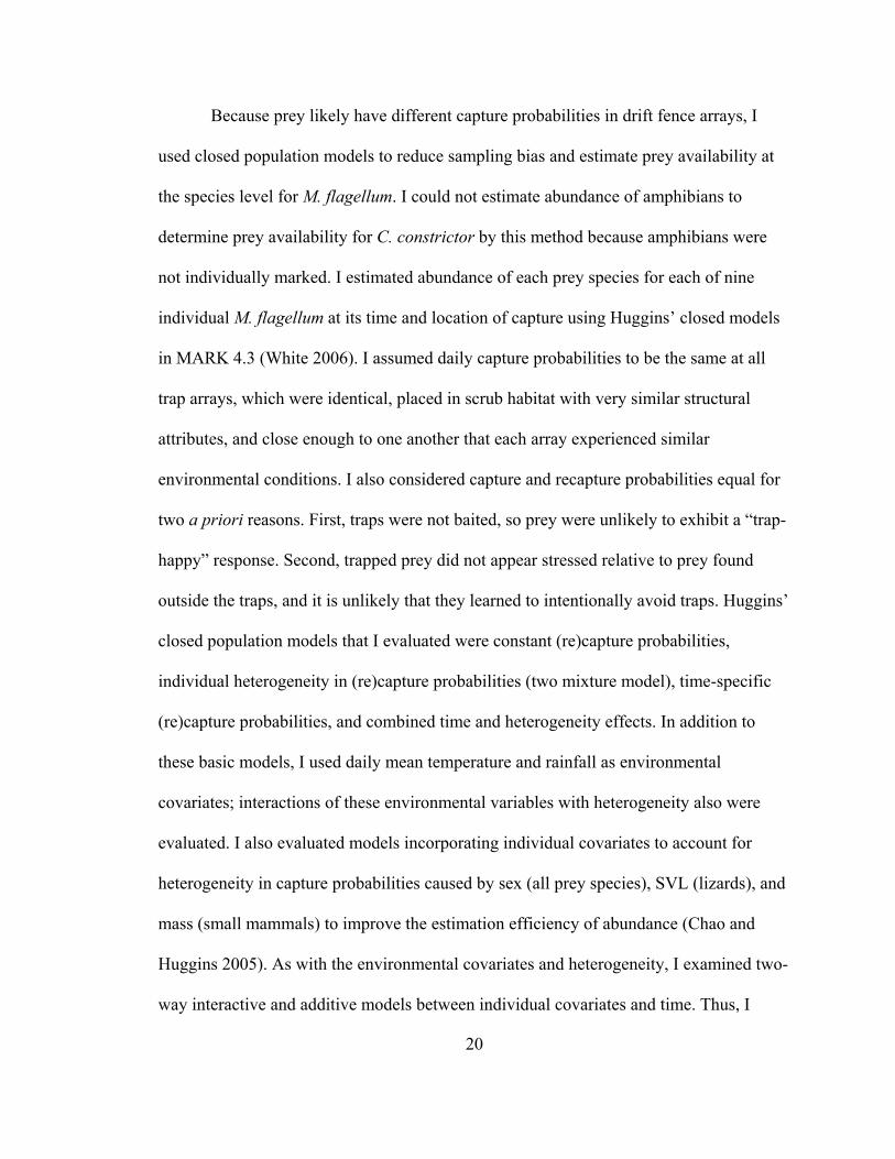
Because prey likely have different capture probabilities in drift fence arrays, I

used closed population models to reduce sampling bias and estimate prey availability at

the species level for M. flagellum. I could not estimate abundance of amphibians to

determine prey availability for C. constrictor by this method because amphibians were

not individually marked. I estimated abundance of each prey species for each of nine

individual M. flagellum at its time and location of capture using Huggins’ closed models

in MARK 4.3 (White 2006). I assumed daily capture probabilities to be the same at all

trap arrays, which were identical, placed in scrub habitat with very similar structural

attributes, and close enough to one another that each array experienced similar

environmental conditions. I also considered capture and recapture probabilities equal for

two a priori reasons. First, traps were not baited, so prey were unlikely to exhibit a “trap-

happy” response. Second, trapped prey did not appear stressed relative to prey found

outside the traps, and it is unlikely that they learned to intentionally avoid traps. Huggins’

closed population models that I evaluated were constant (re)capture probabilities,

individual heterogeneity in (re)capture probabilities (two mixture model), time-specific

(re)capture probabilities, and combined time and heterogeneity effects. In addition to

these basic models, I used daily mean temperature and rainfall as environmental

covariates; interactions of these environmental variables with heterogeneity also were

evaluated. I also evaluated models incorporating individual covariates to account for

heterogeneity in capture probabilities caused by sex (all prey species), SVL (lizards), and

mass (small mammals) to improve the estimation efficiency of abundance (Chao and

Huggins 2005). As with the environmental covariates and heterogeneity, I examined two-

way interactive and additive models between individual covariates and time. Thus, I

21

considered up to 18 models for each prey species available to each snake. I analyzed all

models with covariates using the logit link function, which maps the probability of a

binary response variable (in this case, captured or not captured) from [0,1] to [-∞,+∞]

(Quinn and Keough 2002). If no rain fell during a secondary period, I eliminated all

models that included rainfall from the analysis. Additionally, I did not consider models

that contained more parameters than the number of individual prey of each species

captured during that week because these data were too sparse to estimate the parameters

of more complex models. Thus, only a single model with constant (re)capture probability

could be evaluated for some prey species during certain sampling periods. Because of

sparse recapture data, I could not estimate abundance of all prey species available to the

eleven remaining M. flagellum individuals; therefore, I excluded these individuals from

this analysis.

Studies of diet selection rarely take into account uncertainty associated with the

determination of prey availability. I therefore developed a procedure to account for

uncertainty inherent in estimating the abundance of cryptic, mobile prey. Because my

data were nearly always supported by more than one of the models, I used model

averaged abundance estimates to account for uncertainty in model selection (Burnham

and Anderson 2002). For each snake, I accounted for overall uncertainty in estimates of

prey abundance (that arising from both model selection uncertainty and variance in

abundance estimates for each model) with a two-step resampling procedure in which

1,000 abundance estimates for each prey species were randomly and independently

sampled from each prey species’ distribution of abundance estimates. Model averaging

resulted in a normal distribution of abundance estimates that often included estimates less

22

than the count of captured individuals. To account for the unrealistic nature of abundance

estimates less than the count of individuals captured, I discarded the randomly selected

estimate if it was less than the count, and the random selection of an abundance estimate

was repeated. If the selected estimate was less than the count after three iterations of this

process, I used the count as an abundance estimate for that bootstrap sample. I calculated

the observed ŵi for each of these 1,000 estimates of availability to generate a distribution

of observed ŵi values that reflected the uncertainty inherent in determining the relative

abundances of prey species. To generate a confidence interval for ŵi under the hypothesis

of random selection of prey, I selected the number of prey individuals consumed by the

snake from each of these 1,000 availability estimates 100 times, yielding 100,000

samples for each individual. I analyzed prey selection at the population level as above

using Bi, and tested for statistical significance using Pearson’s χ2 with bootstrapped

confidence intervals.

I calculated niche breadth and niche overlap to compare the foraging

characteristics of the two snakes and place these foraging patterns in a broader ecological

context. I determined niche breadth for each snake species using Hurlbert’s B’ index,

which describes the breadth of the diet relative to the availability of prey in the

environment (Hurlbert 1978). I used Morisita’s C index (Horn 1966) to examine niche

overlap. This index is interpretable as the probability that two prey drawn randomly from

each predator population will be the same species, standardized to account for the

diversity of each predator’s diet (Horn 1966). I established confidence intervals for both

indices by bootstrapping (1,000 random samples). Statistical analyses were conducted

using the programs MARK 4.3 (White 2006), Resampling Stats 5.0.2 (Resampling Stats,

23

Inc., 1999), and R 2.3.1 (R Core Development Team 2006). All means are reported as

mean (±standard error).

RESULTS

Diet Composition

Snakes that contained stomach contents were representative of trapped individuals

for each species. Eighty-one individual M. flagellum were examined for stomach contents

one-hundred thirteen times, and 268 C. constrictor were examined for stomach contents

three hundred times. No sexual size dimorphism in SVL was detected for either species

(M. flagellum: males = 831 ± 61 mm [330 – 1650 mm], females = 806 ± 53 mm [375 –

1520 mm]; W = 840, P = 0.73; C. constrictor: males = 667 ± 15 mm [300 – 1030 mm],

females = 671 ± 15 mm [240 – 1065 mm]; W = 8800, P = 0.82), so sexes were pooled

within species for analysis. The size distribution of individuals containing stomach

contents was not significantly different from the size distribution of all trapped

individuals for each species (M. flagellum: D = 0.20, P = 0.51; C. constrictor: D = 0.11,

P = 0.61). Likewise, the sex ratio of individuals containing stomach contents was not

significantly different from the sex ratio of all trapped snakes of each species (M.

flagellum: G = 0.01, df = 1, P = 0.92; C. constrictor: G = 0.51 df = 1, P = 0.48). Twenty-

one (18.6%) M. flagellum and 59 (28.2%) C. constrictor contained prey. Of these, one

female M. flagellum was not forced to regurgitate, one C. constrictor contained

unidentified organic matter, two C. constrictor could not be forced to regurgitate, and

three gravid female C. constrictor were not forced to regurgitate. Three individual C.

24

constrictor contained prey on more than one occasion. The proportion of individuals of

each species that contained prey was not significantly different (G = 0.53, df = 1, P =

0.47).

Both predator species consumed a variety of prey. At the prey category level, M.

flagellum most frequently consumed lizards, and C. constrictor consumed amphibians

and lizards in nearly equal proportions (Fig. 1). The most frequently consumed lizard in

the diet of M. flagellum was Sceloporus woodi (Florida Scrub Lizard), and the most

frequently consumed mammal was Podomys floridanus (Florida Mouse; Fig. 2). The

most frequently consumed amphibian, lizard, and mammal in the diet of C. constrictor

were Hyla femoralis (Pine Woods Treefrog), Aspidoscelis sexlineata (Six-lined

Racerunner), and Peromyscus polionotus (Oldfield Mouse), respectively (Fig. 2). One C.

constrictor contained anuran legs that could not be identified to species. Individuals of

both snake species consumed relatively few prey, with a maximum of three prey in one

individual M. flagellum and four prey in one individual C. constrictor. Both species had a

mode of one prey item. The distribution of the number of prey items per stomach did not

differ between the two species (Fisher’s exact test, P = 0.80).

Both M. flagellum and C. constrictor consumed prey that were small relative to

their body size. Larger individuals of both species continued to consume the same prey

categories as small snakes, but individuals of both species did not consume mammals

until they reached a minimum size of 725 mm SVL (Fig. 3). Mean relative prey mass of

M. flagellum was 0.098 (±0.032), with a range of 0.008 – 0.27, and mean relative prey

mass of C. constrictor was 0.068 (±0.014), with a range of 0.003 – 0.359. Mean relative

prey mass did not differ between the two snake species (W = 180, P = 0.27), nor did the

25

distribution of relative prey mass differ between them (D = 0.38, P = 0.25). Masticophis

flagellum did not exhibit a significant relationship of snake mass with prey mass (ρ =

0.36, P = 0.39), but C. constrictor did (ρ = 0.42, P = 0.01; Fig. 4). No significant

relationship existed between predator SVL and relative prey mass for either species (M.

flagellum: ρ = -0.36, P = 0.39; C. constrictor: ρ = 0.077, P = 0.66).

Diet Selection

A variety of vertebrate prey species were consumed by and available to individual

M. flagellum and C. constrictor (Tables 1 and 2). Arthropods were present on the site, but

their abundance was not quantified. At the population level, patterns of prey selection for

M. flagellum and C. constrictor differed. At the prey category level, M. flagellum

approached selective predation (n = 20, χ2 = 9.0, P = 0.06), and positively selected

lizards, consumed mammals and snakes in proportion to their availability, and avoided

amphibians (Table 3). Masticophis flagellum selected lizards significantly more than

amphibians and snakes, and selected mammals significantly more than amphibians

(Table 3). Coluber constrictor was not selective at the prey category level (n = 56, χ2 =

2.8, P = 0.45), and consumed prey in proportion to their availability (Table 3). At the

prey species level, M. flagellum selected prey in proportion to their availability regardless

of whether counts (n = 20, χ2 = 3.1, P = 0.43) or abundances (n = 9, χ2 = 0.74, P = 0.97)

were used as estimates of availability, but B-values for some prey species changed

considerably depending upon which method was used to define available resources

(Table 4). Coluber constrictor was selective at the prey species level (n = 55, χ2 = 90, P <

0.01), and positively selected Hyla femoralis while negatively selecting Bufo quercicus

26

(Oak Toad), B. terrestris, and Gastrophryne carolinensis (Eastern Narrowmouth Toad;

Table 5). In pairwise comparisons, C. constrictor selected H. femoralis significantly more

than all other species except Acris gryllus (Southern Cricket Frog), Rana capito (Gopher

Frog), Podomys floridanus, and Peromyscus polionotus, and selected Anolis carolinensis

(Green Anole) significantly more than the B. quercicus.

Niche Breadth and Overlap

The relationship between the niche breadths of the two snake species varied

depending upon the scale at which it was examined. At the level of prey category, M.

flagellum had a narrower niche than C. constrictor, but this difference was not

statistically significant (Table 6). At the prey species level, the opposite pattern was

observed, with M. flagellum exhibiting a significantly broader diet in relation to its

available prey than C. constrictor did (Table 6). Niche overlap between the two predator

species was considerable at both levels of analysis (Table 6).

DISCUSSION

Masticophis flagellum and C. constrictor are selective foragers that consume

relatively small prey. Both species consume a variety of prey, but each is selective at a

different level of taxonomy. Masticophis flagellum positively selects lizards and

mammals, and it consumes prey species within these categories in proportion to their

availability. In contrast, C. constrictor forages opportunistically upon prey categories, but

is selective at the species level, particularly among amphibian species. Thus, foraging by

27

these two snake species occurs by a hierarchical process whereby selection can occur at

different levels of prey taxonomy.

The observed differences in the foraging habits of these two species are somewhat

surprising, given their usual characterization as generalist predators (Ernst and Barbour

1989). Dietary differences between these species cannot be explained by size alone,

because individuals of similar sizes were sampled from both snake species and large

individuals of both species consumed the same prey categories and species that smaller

conspecifics did. Although amphibians have not been reported in the diet of M. flagellum,

they are available to M. flagellum. Therefore, M. flagellum actively avoids consuming

amphibians. In contrast, C. constrictor consumed amphibians more frequently in my

study site than elsewhere (Hamilton and Pollack 1956, Klimstra 1959, Fitch 1963,

Shewchuk and Austin 2001). Because I did not determine that prey were limiting to these

snakes, I were unable assess competition between them. If lizard and mammal prey were

limiting, competition with M. flagellum might explain the greater consumption of

amphibians by C. constrictor in Florida scrub than elsewhere. Alternatively, amphibians

may be more abundant at my site than other locations, and their prominence in the diet of

C. constrictor in Florida scrub may simply reflect relatively high amphibian abundance.

Additional studies of prey limitation and the diet selection of these two snake species

across their geographic ranges are required to evaluate these hypotheses.

Although M. flagellum was selective at the prey category level and C. constrictor

was selective at the prey species level, both predator species consumed lizard and

mammal species in proportion to their availability. Perhaps a general search image and

acceptability of all lizards and mammals as viable prey exists for both species, while C.

28

constrictor discriminates among anuran species. Prey discrimination could potentially

occur at multiple stages of the predation event, including prey detection, prey capture,

prey manipulation, intraoral transport, or even swallowing (Cundall and Greene 2000). It

is currently unknown at which of these stages C. constrictor rejects toxic anurans (Bufo

spp. and G. carolinensis (Garton and Mushinsky 1978, Daly et al. 1987)), or whether

individuals learn to avoid certain species after exposure to toxins. The genus Bufo has

been documented in the diet of C. constrictor (Klimstra 1959, Fitch 1963); however, I

found that C. constrictor avoided Bufo species. Inter- and intraspecific geographic

variation in the toxicity of Bufo and/or geographic variation in the tolerance of

bufodienolides or alkaloids by C. constrictor may occur (Brodie et al. 2002).

Alternatively, C. constrictor may resort to foraging on avoided prey species if more

preferred alternatives are unavailable. Again, detailed studies of prey toxicity, predator

tolerance of toxins, and prey availability are necessary to evaluate these hypotheses.

The consumption of insects, particularly Orthoptera, by C. constrictor is well-

documented (Klimstra 1959, Fitch 1963, Shewchuk and Austin 2001), but I found no

insect prey in the stomachs of C. constrictor. One potential explanation for the absence of

insects in the diet of C. constrictor in Florida scrub is the tendency for eastern C.

constrictor to consume fewer insects than western conspecifics (Fitch 1963). The pattern

of prey consumption by C. constrictor is likely more complicated than this apparent

gradient of reduced consumption of insect prey from west to east suggests. Most studies

of snake diets are conducted without quantifying the availability of prey, which is an

essential component of any comparison of prey selection by free-ranging snakes. Florida

scrub is a nutrient-poor habitat (Myers 1990) with a relatively low abundance of

29

arthropods, many of which appear chemically well-defended against predators (Witz and

Mushinsky 1989, Witz 1990). Because I did not quantify arthropod abundance, I cannot

assess whether C. constrictor in Florida scrub avoids available arthropods or merely

ignores them because of their low abundance. Prey availability is thus not only important

for documenting geographic, temporal, and taxonomic differences in predator diets, but

also to elucidate mechanisms leading to selective predation within populations.

As I predicted, M. flagellum and C. constrictor consume relatively small prey

compared to other macrostomate (large-mouthed) snakes (Cundall and Greene 2000).

Studies of other snake species have demonstrated the capacity of snakes to consume

relatively large prey (Mushinsky 1982, Pough and Groves 1983, Arnold 1993, Cundall

and Greene 2000, Rodriguez-Robles 2002, Greene and Rodriguez-Robles 2003, Gregory

and Isaac 2004). Many species consume prey larger than those ingested by either M.

flagellum or C. constrictor. All species included in Table 3 of Rodríguez-Robles (2002)

had a greater mean relative prey mass than both M. flagellum and C. constrictor, and of

these 13 species, only Boiga irregularis (Brown Treesnake) and Psammodynastes

pulverulentus (Asian Mock Viper) had a lower maximum relative prey mass. Larger

potential prey than those consumed by both snake species, such as Sylvilagus floridanus

(Eastern Cottontail) and Sigmodon hispidus (Cotton Rat), were available in and adjacent

to sampled patches of Florida scrub at my study site, but these prey were likely at or

above the maximum prey size available to each species. A particularly large adult M.

flagellum foraging in pine flatwoods habitat at my study site was observed to consume

adult S. hispidus, which are too large or formidable for all but the largest M. flagellum

(and all C. constrictor) at my site to consume. Although prey mass increased with snake

30

mass for both species, longer snakes did not consume relatively heavier prey. A free-

ranging adult M. flagellum at my study site was observed to consume A. carolinensis,

indicating that large M. flagellum do not drop these small lizards from their diet. My

stomach contents data support this observation: adults of both snake species continued to

consume prey species and categories consumed by smaller juvenile conspecifics.

Therefore, both species exhibit an ontogenetic telescope (Arnold 1993), rather than an

ontogenetic shift in diet (Mushinsky 1982).

Masticophis flagellum and C. constrictor are relatively abundant in Florida scrub

habitat, and previous research suggests that they may exert a strong influence on the

dynamics of small, isolated populations of prey occurring in scrub fragments. In

particular, S. woodi has lower survivorship in small patches of scrub; smaller habitat

patches may suffer increased predation rates by snakes (Hokit and Branch 2003b). In

addition to the positive relationship between patch size and survivorship, McCoy et al.

(2004) observed density-dependent mortality of S. woodi associated with the presence of

and observed predation by both M. flagellum and C. constrictor. My findings are

consistent with these observations. Both predator species consume prey opportunistically

at some level, and opportunistic predators likely exert a direct density-dependent effect

on prey (such as that observed by McCoy et al. [2004]). Although these predators are

unlikely to exhibit a numerical response (via increased reproductive rates) to any single

prey species’ abundance, aggregative movement to areas of high prey density by these

wide-ranging snakes could exert a strong influence on local prey dynamics. If M.

flagellum does not form a species-specific search image, as my data suggest, it may have

a hyperbolic functional response that could lead to the extirpation of prey that occur at

31

low densities (Turchin 2003). Effects of predation by M. flagellum may be especially

strong on S. woodi and P. floridanus, which are both important dietary components of M.

flagellum and precinctive to Florida scrub. Knowledge of the foraging behavior and diet

selection of predators may be important for the conservation of these rare prey species.

In summary, I found that M. flagellum and C. constrictor are selective foragers

that consume relatively small prey. As I hypothesized, both M. flagellum and C.

constrictor consume small prey relative to other snakes. In contrast to my hypotheses,

both species were selective of prey at some level. Masticophis flagellum positively

selected lizards and mammals, but consumed species within these categories in

proportion to their availability. Coluber constrictor consumed amphibians, lizards, and

mammals in proportion to their availability, but within the amphibian category positively

selected H. femoralis and negatively selected the B. quercicus, B. terrestris, and G.

carolinensis. By defining availability separately for each individual snake, I was able to

incorporate gape limitation and account for spatial and temporal variation in prey

availability in my analyses of prey selection. Mechanisms underlying geographic,

temporal, and interspecific variation in predator diets can be better elucidated by

examining prey availability and selection at the level of the individual.

32

Table 1. Prey Species Consumed by and Available to Individual Masticophis flagellum. Abbreviations used are: ID = snake identification number, SVL = snake snout-vent length (in mm), SC (No.)

= prey species found in stomach (number of prey of that species), Acar = Anolis carolinensis, Asex = Aspidoscelis sexlineata, Swoo = Sceloporus woodi, Pflo = Podomys floridanus, and Ppol =

Peromyscus polionotus. * - Abundance was estimated for each species using model-averaged parameters from Huggins’ closed models with capture probability held constant across trap arrays. † -

Snake was included in diet selection analysis using abundance of prey as estimate of availability. ‡ - Numbers in brackets indicate prey that were sampled in the same array during the same week as

the snake, but were too large for the snake to consume based upon snake and prey measurements.

Snake Prey Available (Count) Prey Available (Abundance [SE])*

ID SVL SC (No.) Acar Asex Swoo Pflo Ppol Acar Asex Swoo Pflo Ppol

40F† 878 Asex (1) 9 9 30.4 (17.6) 23.5 (9.9)

E21† 1650 Asex (1) 8 2 1 19.5 (8.7) 4.9 (3.0) 2.6 (2.7)

258 920 Swoo (1) 3 3 [1]‡ NA 7.1 (6.3) [2.6 (2.5)]

519† 580 Swoo (1) 5 [1] 8.3 (4.3) [2.7 (3.5)]

7† 475 Swoo (2) 7 [2] 296 (920) [6.2 (6.5)]

76F 1220 Pflo (1) 1 2 3.3 (3.0) NA

10 555 Acar (1) 1 6 NA 20.0 (9.7)

953 955 Acar (2) 5 1 9 NA 4.6 (4.7) 26.6 (12.0)

Swoo (1)

534† 665 Swoo (1) 7 20.0 (9.7)

867 600 Swoo (1) 1 2 2 [1] 1 NA 12.5 (11.7) 2.1 (1.7) [2.0 (1.5)] 3.4 (4.6)

11 585 Acar (1) 2 1 3 [4] NA 7.2 (8.9) 6.4 (3.1) [6.7 (2.7)]

94A† 1090 Pflo (1) 1 4 2.1 (1.7) 5.0 (2.5)

406† 1070 Swoo (1) 1 1 12 4.8 (6.0) 2.2 (1.7) 17.3 (4.0)

15 400 Acar (1) 3 4 4 1 9.6 (10.4) 1 2.7 (6.5) 18.9 (13.5) NA

D50 965 Swoo (1) 2 2 4 [2] 2 NA 14.3 (19.0) 6.8 (3.6) [2.9 (1.4)] 2.7 (1.1)

33

Table 1 (Continued).

Snake Prey Available (Count) Prey Available (Abundance [SE])*

ID SVL SC (No.) Acar Asex Swoo Pflo Ppol Acar Asex Swoo Pflo Ppol

29 665 Asex (1) 1 4 [8] 1 NA 8.3 (4.7) [10.0 (1.8)] 2.7 (2.6)

048† 965 Swoo (1) 1 5 [4] 3 3.1 (3.0) 12.2 (9.7) [5.1 (1.3)] 7.5 (1.7)

143 1150 Asex (1) 1 1 2 5 2 NA NA 4.9 (3.1) 6.6 (1.6) 4.9 (3.9)

A29 930 Ppol (1) 5 1 18.0 (9.7) NA

32† 750 Swoo (1) 3 [1] 4.4 (2.7) [1.2 (0.6)]

34

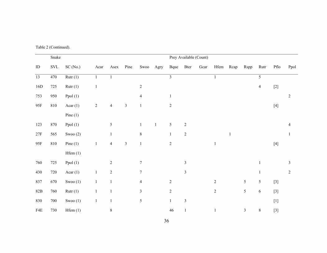
Table 2. Prey Species Consumed by and Available to Individual Coluber constrictor. Abbreviations used are: ID = snake identification number, SVL = snake

snout-vent length (in mm), SC (No.) = prey species found in stomach (number of prey of that species), Acar = Anolis carolinensis, Asex = Aspidoscelis

sexlineata, Pine = Plestiodon inexpectatus, Swoo = Sceloporus woodi, Agry = Acris gryllus, Bque = Bufo quercicus, Bter = B. terrestris, Gcar = G.

carolinensis, Hfem = Hyla femoralis, Rcap = Rana capito, Rspp = Rana catesbeiana + R. grylio, Rutr = Rana utricularia, Pflo = Podomys floridanus, and

Ppol = Peromyscus polionotus. * - Numbers in brackets indicate prey that were sampled in the same array during the same week as the snake, but were too

large for the individual to consume based upon snake gape and prey measurements. † - Snake was not included in prey species-level analyses because

stomach contents could not be identified to the species level.

Snake Prey Available (Count)

ID SVL SC (No.) Acar Asex Pine Swoo Agry Bque Bter Gcar Hfem Rcap Rspp Rutr Pflo Ppol

2 380 Swoo (1) 1 8 1

A 370 Swoo (1) 1 2 [2]*

C35 736 Swoo (2) 4

B11 742 Acar (1) 2 9 1 4 1 13

671 805 Rutr (1) 1 9 1 4 1 14

44F 985 Rutr (1) 1 9 1 4 1 14

274 910 Asex (1) 1 7 8 7

F66 655 Asex (1) 2 29 2 1 1 1

155 770 Swoo (1) 5 5 4 [1]

35




650 660 Asex (1) 17 6 1 1 3 10

7 533 Rutr (1) 1 6 2 3 5 5 5 7

53F 720 Acar (2) 2 5 14 9 1 1 1 2 [1]

Asex (1)

F0A 560 Rutr (1) 7 2 11 6 5 2

8 530 Asex (1) 8 2 11 6 5 1

F15 810 Hfem (1) 2 4 1 1 8 2 [1]

E22 870 Asex (1) 2 1 1 4 2 2

F2F 710 Hfem (1) 2 3 6 8 1 1 1

45D 960 Pflo (1) 3 1 2 1 1 2

15 395 Hfem (1) 7 3 2 3 [2] 1 1 [1]

20 400 Hfem (3) 2 8 1 2 3 [6] 2

21 400 Acar (1) 2 4 3 [1]

24 380 Hfem (1) 1 1 3 2 4

25 360 Hfem (1) 5 2 2 1 [2]

36




13 470 Rutr (1) 1 1 3 1 5

16D 725 Rutr (1) 1 2 4 [2]

753 950 Ppol (1) 4 1 2

95F 810 Acar (1) 2 4 3 1 2 [4]

Pine (1)

123 870 Ppol (1) 5 1 1 5 2 4

27F 565 Swoo (2) 1 8 1 2 1 1

95F 810 Pine (1) 1 4 3 1 2 1 [4]

Hfem (1)

760 725 Ppol (1) 2 7 3 1 3

430 720 Acar (1) 1 2 7 3 1 2

837 670 Swoo (1) 1 1 4 2 2 5 5 [3]

82B 760 Rutr (1) 1 1 3 2 2 5 6 [3]

830 700 Swoo (1) 1 1 5 1 3 [1]

F4E 730 Hfem (1) 8 46 1 1 3 8 [3]

37




39 835 Rutr (1) 1 3 9 5 4 1 3 [2] 1

727 720 Hfem (1) 2 1 2 1 5 2 1 1 1 [1]

30E 755 Rspp (1) 5 1 4 1 1

93A 780 Asex (1) 1 10 1 5 1 1

143 605 Asex (1) 4 1 3 7 1 1 1 [2]

D39 755 Hfem (1) 3 2 2 8 2 [1] 3 1 1 [2]

91A 790 Asex (1) 1 5 2 2 1 [3]

42 750 Acar (1) 2 6 1 3

Hfem (3)

46 320 Acar (1) 1 5 2 1 2

Hfem (1)

49 740 Rspp (1) 1 1 1 3 5 1 [3]

67 730 Rspp (1) 1 3 1 28 3 [3]

A0F 790 Asex (1) 1 4 [9] 1

20 770 Acar (1) 1 6 3 1 [1]

38

Table 2 (Continued)



97 745 Asex (1) 1 1 2 [5] 2

106 710 Swoo (1) 2 3 4 5 2 2 1 1 [2]

143 690 Asex (1) 1 9 1 6 2 [4]

B22 670 Rcap (1) 2 30 18 20 3 6 28

926 610 Hfem (1) 5 3 4 8 [2] 1 2 1

A06 895 Agry (1) 1 4 1 1 3 2

Prey Category Available (Count)

Amphibian Lizard Snake Turtle Bird Mammal

63† 755 Amp (1) 17 2 1 1

39

Table 3. Manly’s Standardized Selection Ratios (B) for Prey Categories Selected by Masticophis flagellum and Coluber

constrictor. P-values were obtained from 1,000 bootstrap samples. Superscripts indicate significant pairwise differences in

selection of prey categories.

Masticophis flagellum (n = 20) Coluber constrictor (n = 56)

Prey Category B P B P

Amphibians 0.000c <0.01 0.244 0.65

Lizards 0.54a <0.01 0.301 0.34

Snakes 0.000bc 0.37 0.000 0.19

Turtles None Available 0.000 0.73

Birds None Available 0.000 0.83

Mammals 0.46ab 0.13 0.455 0.05

40

Table 4. Manly’s Standardized Selection Ratios (B) for Prey Species Selected by Masticophis flagellum. Estimates of prey

availability for individual snakes were obtained by counts and by estimating prey abundances using model-averaged Huggins’

closed population models. P-values were obtained from 1,000 bootstrap samples for counts, and 100,000 bootstrap samples for

abundances.

Counts (n = 20) Abundances (n = 9)

Prey Species B P B P

Anolis carolinensis 0.371 0.10 0.00 0.41

Aspidoscelis sexlineata 0.152 0.54 0.38 0.44

Sceloporus woodi 0.157 0.40 0.28 0.81

Podomys floridanus 0.183 0.54 0.35 0.64

Peromyscus polionotus 0.138 0.80 0.00 0.56

41

Table 5. Manly’s Standardized Selection Ratios (B) for Prey Species Selected by Coluber

constrictor. P-values were obtained from 1,000 bootstrap samples. Superscripts indicate

significant pairwise differences in selection of prey species. n = 55.

Prey Species B P

Hyla femoralisa 0.213 <0.01

Acris gryllusabc 0.142 0.50

Rana capitoabc 0.113 0.64

Rana catesbiana and Rana gryliobc 0.060 0.79

Rana utriculariabc 0.049 0.43

Gastrophryne carolinensisbc 0.000 <0.01

Bufo terrestrisbc 0.000 <0.01

Bufo quercicusc 0.000 <0.01

Anolis carolinensisb 0.100 0.46

Aspidoscelis sexlineatabc 0.040 0.10

Sceloporus woodibc 0.040 0.06

Plestiodon inexpectatusbc 0.038 0.48

Podomys floridanusabc 0.118 0.69

Peromyscus polionotusabc 0.087 0.69

42

Table 6. Dietary Niche Breadth (Hurlbert’s B’) and Niche Overlap (Morisita’s C) of Masticophis flagellum and Coluber

constrictor. Confidence intervals for Hurlbert’s B’ represent expected values for an opportunistic predator that consumes prey in

proportion to its availability.

Niche Breadth Niche Overlap

Level of Analysis Snake Species B’ 95% CI C 95% CI

Prey Category Masticophis flagellum 0.689 0.662-0.991 0.728 0.525-0.861

Coluber constrictor 0.956 0.751-0.992

Prey Species Masticophis flagellum 0.877 0.649-0.967 0.755 0.431-0.893

Coluber constrictor 0.431 0.682-0.916

Figure 1. Occurrence of Prey Categories Consumed by Masticophis flagellum and

Coluber constrictor Expressed as a Proportion of Individuals of Each Species that

Consumed Each Prey Category. Numbers above bars indicate the number of individuals

of each prey category that were consumed. Proportions for C. constrictor do not sum to

one because four individuals contained both amphibians and lizards in their stomachs.

43

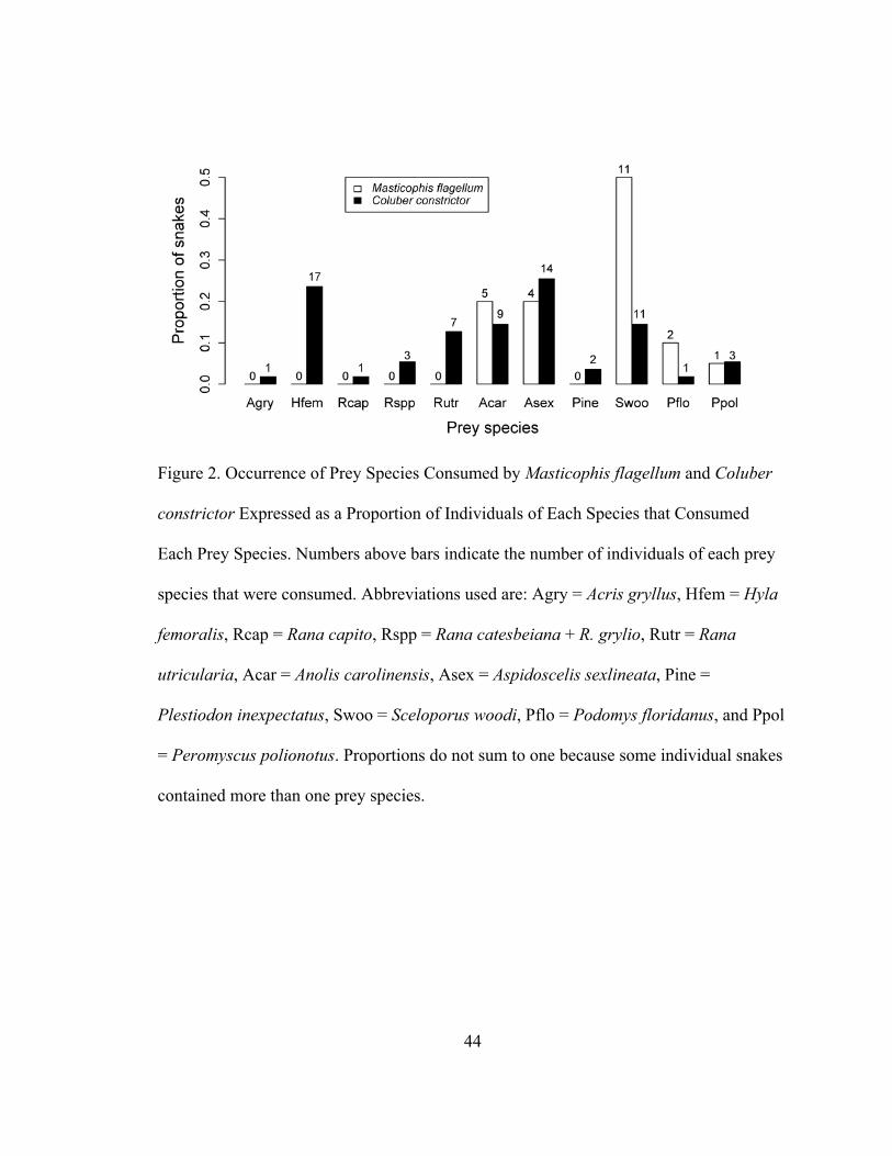
Figure 2. Occurrence of Prey Species Consumed by Masticophis flagellum and Coluber

constrictor Expressed as a Proportion of Individuals of Each Species that Consumed

Each Prey Species. Numbers above bars indicate the number of individuals of each prey

species that were consumed. Abbreviations used are: Agry = Acris gryllus, Hfem = Hyla

femoralis, Rcap = Rana capito, Rspp = Rana catesbeiana + R. grylio, Rutr = Rana

utricularia, Acar = Anolis carolinensis, Asex = Aspidoscelis sexlineata, Pine =

Plestiodon inexpectatus, Swoo = Sceloporus woodi, Pflo = Podomys floridanus, and Ppol

= Peromyscus polionotus. Proportions do not sum to one because some individual snakes

contained more than one prey species.

44

Figure 3. Relationship between Prey Category and Predator Size (Snout-vent Length) for

Masticophis flagellum and Coluber constrictor. Each point represents a single snake.

Four individual C. constrictor that contained both amphibians and lizards appear in both

categories.

45

Figure 4. Ln-transformed Prey Mass as a Function of Ln-transformed Snake Mass for

Masticophis flagellum (dashed line; adjusted R2 = -0.067, F(1,6) = 0.56, P = 0.48) and

Coluber constrictor (solid line; adjusted R2 = 0.36, F(1,34) = 20.44, P < 0.0001). Only

individual snakes that contained relatively intact prey were included in this analysis (M.

flagellum: n = 8, C. constrictor: n = 36).

46

47

Masticophis flagellum (Coachwhip) Positively Selects Florida Scrub Habitat at

Multiple Spatial Scales

The appropriate use of space by animal populations is vital to their growth and

persistence. In particular, prudent choice of foraging sites, refugia, and movement paths

by individuals is crucial to ensure that they obtain adequate food and avoid predators and

environmental extremes. Studies of habitat selection by animals provide this essential

information about requirements for survival and can inform conservation about animal

populations (Manly et al. 2002). In particular, understanding the mechanisms underlying

habitat selection can help to identify factors limiting the occurrence or abundance of

populations (Blouin-Demers and Weatherhead 2001b, Pringle et al. 2003), and can help

identify sources of population declines (Waldron et al. 2006).

Masticophis flagellum (Coachwhip) is a large, active snake found throughout the

southern United States and northern Mexico (Ernst and Barbour 1989). Masticophis

flagellum has large home ranges, and makes frequent long-distance movements (Secor

1995, Dodd and Barichivich 2007, Johnson et al. 2007). Masticophis flagellum occurs in

many habitats (Carr 1940, Ernst and Barbour 1989, Tennant 1997), but recent studies

indicate that M. flagellum primarily uses xeric, open-canopied habitats (Dodd and

Barichivich 2007, Johnson et al. 2007). Masticophis flagellum actively searches for prey

and captures it by rapid pursuit (Secor 1995). The active habits of M. flagellum are

accompanied by a high metabolic rate and relatively frequent feeding (Secor and Nagy

48

1994, Secor 1995). Because of its high metabolic rate and frequent movements, the

spatial ecology of M. flagellum may be strongly tied to prey abundance.

Our goals in this study were to document the spatial ecology and habitat selection of M.

flagellum in central Florida. Based upon previous studies (Dodd and Barichivich 2007,

Johnson et al. 2007), I hypothesized that these vagile snakes would select xeric habitats,

which primarily consisted of Florida scrub at my study site. Because Florida scrub habitat

on my study site occurred in patches, I predicted that M. flagellum at my site would

exhibit large home range sizes and long-distance movements between patches. I further

hypothesized that M. flagellum would select Florida scrub patches based upon the prey

abundance in each patch.


Study Site

I conducted this research at the Lake Arbuckle tract of the Lake Wales Ridge


Longitude). The site consists of a series of patches of xeric Florida scrub habitat and

wetlands in a matrix of mesic, and more densely vegetated, pine flatwoods habitat (Fig.

5). Wetlands consisted primarily of depression marshes that were seasonally inundated

and larger forested wetlands. Depression marshes were dominated by Monocots,

primarily Panicum hemitomon; some marshes also contained small shrubs (Salix spp. and

Hypericum spp.). Forested wetlands were primarily bayheads and sloughs dominated by

Gordonia lasianthus and Persea palustris.

49

Florida scrub is a rare, xeric habitat that contains many precinctive organisms

(Myers 1990, McCoy and Mushinsky 1992). Florida scrub at the site was primarily oak

scrub, and was dominated by a 0.5-1.5 m high midstory of Quercus spp., Lyonia spp.,

Sabal etonia and Serenoa repens. Canopy cover in the Florida scrub was generally less

than ten percent, and was dominated by Pinus elliottii. Groundcover in the Florida scrub

was primarily bare sand and leaf litter with little herbaceous vegetation. A few xeric areas

on the site were sandhill habitat, which was distinguishable from Florida scrub by its

increased cover of herbaceous vegetation (particularly Aristida and Andropogon spp.),

and the presence of Quercus laevis and/or Pinus palustris.

Pine flatwoods habitats covered the greatest amount of area at the site. These

habitats had a denser P. elliottii canopy than the Florida scrub, and also had a thicker

groundcover. Two distinct communities were evident in the pine flatwoods. One

community was dominated by a thick groundcover of Panicum abscissum, and had a

sparse midstory consisting of scattered stands of S. repens and Ilex glabra. The other

community was more typical of flatwoods habitats, and consisted of a midstory

dominated by S. repens, Lyonia lucida, and Vaccinium myrsinites. The groundcover in

the “typical” pine flatwoods community consisted of diverse graminoids and forbs

occurring at low densities. Because the structure of these two communities was distinct,

hereafter I distinguish them as cutthroat (after the common name of P. abscissum) and

pine flatwoods, respectively.

50

Field Methods

I used radio telemetry to determine the spatial ecology and habitat selection of M.

flagellum. I captured individuals opportunistically by hand or in drift fence/funnel

trap/pitfall trap arrays installed in patches of Florida scrub habitat from March, 2004 to

August, 2005. I transported individuals weighing greater than 320 g to the University of

South Florida for surgical implantation of radio transmitters. I surgically implanted an 8 g

Holohil SI-2 radio transmitter (Holohil Systems, Ltd. Carp, Ontario, Canada) within the

coelom of each individual using standard procedures (Reinert and Cundall 1982). I

allowed individuals to recover in the laboratory overnight, and released each where it was

captured the day following surgery. I did not monitor individuals for the first week after

release to avoid disturbance and allow them to heal.

I physically located individuals as frequently as possible, with a maximum

frequency of one location per day. From March through October, I located each

individual an average of four times per week. From November through February, I

reduced the frequency of relocations to once or twice per week, depending upon the

observed frequency of movement of individuals. Most locations took place during

daylight hours because M. flagellum is primarily diurnal (Ernst and Barbour 1989), but I

varied the time of day at which I located individuals. I systematically selected the first

individual located to avoid locating the same individual at the same time each day, and

determined the order of relocations based upon the proximity of individuals to my current

position. I collected data using a Trimble GeoXT handheld GPS (Trimble, Sunnyvale,

California, USA), and offset the location of the individual when it was aboveground to

51

avoid disturbance to the individual. All locations were differentially corrected in the

laboratory to improve the precision of locations.

I described habitat characteristics in the immediate vicinity of the observed

individual. I categorized habitat as Florida scrub, sandhill, pine flatwoods, cutthroat,

marsh, swamp, and pasture. If the individual was located in Florida scrub habitat, I

recorded the patch of Florida scrub in which the individual was found. I also determined

the behavior of individuals at each location. I categorized behavior as basking, resting,

hiding, moving, fleeing, foraging, or mating. Basking was defined as the individual lying

motionless with greater than fifty percent of its body in direct sunlight. Resting was

similar to basking, except that the body of the individual was primarily in shade. Hiding

included locations where the individual was underground or mostly concealed beneath

leaf litter. I considered an individual to be moving if its locomotion was at a relatively

slow rate of speed, with no obvious searching or foraging behavior. Fleeing individuals

were moving rapidly for short distances, usually because of my approach. Foraging

individuals exhibited extensive searching behavior (tongue-flicking with extensive lateral

movements of the head) or evidence of prey pursuit, prey capture, or the process of prey

ingestion. I did not include digestion as a foraging behavior, but generally categorized

individuals with a food bolus as hiding, resting, or basking. Mating individuals included

any of the phases of courtship, including tactile-chase, tactile-alignment, and intromission

and coitus (Gillingham 1987).

To determine if prey abundance influenced the spatial ecology and habitat

selection of M. flagellum, I monitored the abundance of its prey. In particular, I focused

on the abundance of three lizard species (Anolis carolinensis [Green Anole], Aspidoscelis

52

sexlineata [Six-lined Racerunner], and Sceloporus woodi [Florida Scrub Lizard]) and two

small mammal species (Peromyscus polionotus [Oldfield Mouse] and Podomys

floridanus [Florida Mouse]) documented in the diet of M. flagellum at my study site

(Halstead et al. In review). I sampled all prey using a total of 13 drift fence/pitfall/funnel

trap arrays installed in nine focal Florida scrub patches. I installed one trap array in each

of seven patches (1.5 – 12.6 ha), two trap arrays in one patch (40 ha), and four trap arrays

in the remaining patch (170 ha). I opened trap arrays and checked them daily for seven

consecutive days, then closed them for 21 consecutive days as part of a robust mark-

recapture design (Pollock 1982). I sampled prey from March 2004 to June 2006 for a

total of 20 primary periods. Traps were closed from December 2004 to February 2005

and again from November 2005 to March 2006 because of unacceptably high mortality

rates of trapped small mammals caused by cold overnight temperatures. I uniquely

marked each captured lizard using toe clips (Waichman 1992), and each captured small

mammal using individually numbered size 1005-1 Monel ear tags (National Band and

Tag Co., Newport, KY, USA). All captured individuals were released one meter outside

the trap array immediately after processing.

Analytical Methods

Unless otherwise indicated, I used the individual as the sampling unit for all

analyses. To determine whether an estimate of home range was applicable to M.

flagellum, I evaluated movement paths of individuals for their fit to a random walk

model, using subsequent locations only if they were greater than three meters apart to

avoid spatial autocorrelation. The random walk model is appropriate for relatively

53

infrequent locations, because they lack the correlation in move direction found in actual

movement paths (Turchin 1998). The random walk model was strongly rejected for each

individual (Fig. 6), and indicated that M. flagellum movement is bounded within a home

range. Therefore, I proceeded with analyses appropriate to an organism whose

movements primarily occur within a bounded home range.

I calculated home range sizes of M. flagellum by multiple techniques. I used the

100% minimum convex polygon (MCP) because of its historic use and for analyses of

home range and habitat selection (see below). I also calculated the 95% kernel utilization

distribution to estimate home range area, and the 50% kernel utilization distribution

estimate to estimate core activity area. Kernel utilization distributions have the advantage

of making use of all locations and describe the intensity of space use (Worton 1989,

Kernohan et al. 2001). I calculated the kernel utilization distribution on a 100 x 100 grid

for each individual, and used the ad hoc method of bandwidth selection because of

convergence problems encountered when selecting the bandwidth by least squares cross-

validation. Home ranges were calculated using the package “adehabitat” for R (Calenge

2006).

To determine the vagility of M. flagellum, I calculated mean daily displacement. I

divided distance between all consecutive locations divided by the number of days

between locations for each individual. This analysis included locations where the snake

did not move, or moved less than three meters, between relocations. I also calculated the

displacement between “biologically” independent locations. I defined biologically

independent locations as those greater than three meters apart that did not include ecdysis

(indicated by dull appearance, inactivity, and cloudy, bluish eyes) or digestion of large

54

meals (indicated by the presence of a food bolus). My definition of biological

independence was not equal to spatial independence of locations. The analysis of

independent locations provides a measure of the vagility of active snakes. I also

calculated daily displacement for moves beginning and ending within a patch of Florida

scrub and for all other habitats combined. I tested for differences in mean daily

displacement between habitats with a paired t-test to determine if individuals moved

greater distances while in other habitats than in Florida scrub.

I examined habitat selection at three scales (Johnson 1980). The first scale I

examined was the selection of home ranges within the study site (second-order selection

[Johnson, 1980]). For this scale of selection, I defined habitat availability as the area of

each of seven habitat categories (marsh, swamp, cutthroat, pine flatwoods, sandhill,

Florida scrub, and pasture) within the 100% MCP enclosing all snake locations (Fig. 5). I

defined use separately for each individual as the area of each habitat category within the

individual’s 100% MCP home range. I used the MCP home range because at this scale of

analysis, I was interested in the selection of the home range boundaries, rather than the

intensity of use within that home range. This definition better fit my conceptualization of

second-order selection than other methods of delimiting the home range. For both use and

availability, I calculated the area of each habitat based upon a combination of soils and

satellite imagery of the study site using the X-Tools Pro extension in ArcGIS 9.0 (ESRI,

Redlands, California, USA). Ground-truthing indicated that the combination of soils and

satellite imagery was a good approximation to the delineation of habitats in the field.

I calculated the selection of habitat at this scale using the selection ratio, ŵij

(Manly et al. 2002). I tested for differences in the selection of home ranges by

55

individuals, non-random selection by at least some individuals, and overall selection of

habitat across individuals using the log-likelihood goodness of fit statistic (G2). I

calculated ŵi for each habitat as the average of the ŵij taken across individuals, excluding

individuals for which the habitat was not available. To determine if the selection of each

habitat was nonrandom, I compared my estimate of ŵi to one (the expected value under

the null hypothesis of use in proportion to availability) with a one-sample t-test. To

determine if each habitat was selected significantly more or less than every other habitat,

I compared the ŵi with a two-sample t-test with Welch’s correction for unequal

variances. I calculated Manly’s standardized selection ratios (Bi) from the ŵi, because Bi

is interpretable as the estimated probability that habitat i would be the next habitat

selected if all habitats were equally available (Manly et al. 2002).

In addition to the selection of a home range, I examined the selection of habitats

within the home range (Johnson 1980). I defined availability separately for each

individual as the proportion of each individual’s 100% MCP home range comprised of

each habitat category. At this scale, I used the MCP home range because it allowed us to

achieve greater independence of available habitat and the intensity of use than would a

kernel utilization distribution. Use was defined as the count of independent locations for

each individual in each habitat category.

I analyzed the selection of habitats within the home range using Poisson

regression. For each individual, I used habitat availability as a rate parameter in the

Poisson regression model under the null hypothesis that the count of locations within

each habitat would be proportional to the area of each habitat found within the

individual’s home range. I fit several alternative models, including no habitat selection,

56

constant selection of habitat by all individuals, and selection of habitat varying among

individuals. In addition to these models, I also evaluated models that constrained the

differences in habitat selection among individuals to be a function of sex or snout-vent

length (SVL). Because I used non-nested models, I selected the best-fit model using

Akaike’s An Information Criterion corrected for small sample sizes, AICc (Burnham and

Anderson 2002). After choosing a best-fit model, I calculated the Resource Selection

Function (RSF) for each habitat for each individual using the coefficients of the fitted

model (Manly et al. 2002). I then calculated ŵ for the reference individual and category

(which by definition had an RSF of one), and multiplied each RSF by this value to

determine each of the ŵij. I determined the statistical significance of the ŵi and

differences in selection between habitats using t-tests as above.

I used log-linear modeling and correspondence plots to determine if the use of

certain habitats was related to snake behavior. I used all locations for this analysis under

the assumption that behaviors observed at consecutive locations were independent,

regardless of spatial location. I also pooled observations across individuals, and excluded

data from habitats or behaviors with fewer than twenty observations. Independence of

behavior and habitat was assessed with log-linear models. Association among specific

behaviors and habitats was examined graphically with a correspondence plot.

We also examined habitat selection at a level between third- and fourth-order

selection (Johnson 1980). In this case, I examined the selection of nine focal Florida

scrub patches for which I estimated the abundance of the prey of M. flagellum (Halstead

et al. In review) using mark-recapture techniques (see below). For this scale, I defined

availability as the proportion of each individual’s MCP that consisted of each sampled

57

patch of Florida scrub. I defined use as the count of locations in each of these patches.

Only nine individuals with locations in more than one focal patch were used for this

analysis. To determine if prey abundance affected the space use of snakes, I examined

patterns of patch selection as a function of lizard abundance, mammal abundance, total

prey (lizard plus mammal) abundance, and S. woodi abundance. I examined the influence

of the abundance of S. woodi individually because it is precinctive to Florida scrub and is

a common item in the diet of M. flagellum (Halstead et al. In review).

We estimated prey abundances in each focal patch using Jolly-Seber mark-

recapture models. For each prey species, I combined capture histories from each seven

day secondary period prior to analysis. I fit the POPAN formulation of Jolly-Seber

models using Program MARK 4.3 (White, 2006). I modeled capture probability as

constant (p•) or time-varying (pt) for each species. I assumed weekly capture probabilities

to be the same at all trap arrays, which were identical, were placed in Florida scrub

habitat with very similar structural attributes, and were in close proximity to one another,

so that each array experienced similar environmental conditions. I modeled monthly

survival rate as constant (Φ•), array-specific (Φg), time-varying (Φt), and interactive and

additive effects of array and time (Φg*t, and Φg+t, respectively). Likewise, I modeled the

monthly probability of entry of individuals into the population as constant (pent•), array-

specific (pentg), time-varying (pentt), and interactive and additive effects of array and

time (pentg*t and pentg+t, respectively). I fit all possible combinations of capture

probability, survival rate, and probability of entry for all prey except A. carolinensis and

P. polionotus. Too few individuals of these species were captured to estimate the

parameters of models with multiple interactive and additive terms, so I did not attempt to

58

fit models containing these terms to data from these two species. For each prey species, I

used the model with the lowest AICc to estimate abundance in each patch of Florida scrub

for each month. For each individual M. flagellum, I estimated the mean monthly

abundance of each prey species in each patch within the individual’s MCP home range

over the time period during which the individual was tracked.

Similar to my analysis of habitat selection, I used Poisson regression to examine

Florida scrub patch selection. I fit Poisson rate models including no patch selection,

constant selection of patches across individuals, and patch selection varying among

individuals. In addition to these basic models, I constrained patch selection by individuals

to be a function of sex or SVL. I also constrained patch selection to be a function of S.

woodi abundance, lizard abundance, mammal abundance, and total prey (lizard plus

mammal) abundance. Finally, I evaluated a model that allowed selection of patches to be

an interactive function of snake SVL and mammal abundance because mammals were

much larger prey than lizards and maximum prey size in snakes is a function of gape size

(Miller and Mushinsky 1990, Cundall and Greene 2000), which is strongly correlated

with SVL in M. flagellum (n = 18, Gape = 0.126*SVL + 26.9, R2 = 0.93, F(1,16) = 234, P <

0.001). I selected a best-fit model using AICc, and calculated ŵij as above for habitat

selection. I determined the statistical significance of the ŵi and differences in selection

between habitats using t-tests as above.

Statistical analyses were conducted using the programs MARK 4.3 (White 2006)

and R 2.3.1 (R Core Development Team 2006). Descriptive statistics are reported as

mean (±standard error), and statistical significance was set at α = 0.05.

59

RESULTS

I located 14 individual M. flagellum a total of 1556 times from March 2004

through May 2006 (Table 7). Nine individuals were female and five were male. I

eliminated 167 locations that were less than three meters from the previous location,

which was primarily caused by individuals in ecdysis, digesting large meals, or inactive

because of cool temperatures during the winter.

The adult M. flagellum in my study had relatively large home ranges (Fig. 7).

Mean 95% fixed kernel utilization distribution home range area for the population was

177.07 (±41.24) ha (Table 8). Mean core activity area was 38.42 (±8.33) ha. Males and

females did not differ in home range area (males: 212.73 [±52.38]; females: 157.26

[±58.31]; W = 33, P = 0.19) or core activity area (males: 51.47 [±13.87]; females: 31.17

[±10.19]; W = 34, P = 0.15). Home range area was positively correlated with SVL (ρ =

0.55, P = 0.043), but was not related to the tracking period duration (ρ = 0.21, P = 0.46)

or number of locations (ρ = 0.40, P = 0.15) of the individual. Home range size was

negatively correlated with proportion of Florida scrub habitat found within the home

range (ρ = -0.56, P = 0.042).

Adult M. flagellum made relatively long movements between relocations. Mean

daily displacement was 132.1 (±8.3) m for all locations, and 153.0 (±9.8) m for

biologically independent locations (Table 9). Males and females did not differ in mean

daily displacement (males: 170 [±23] m; females: 114 [±8] m; t = 2.04, df = 8.47, P =

0.074). Mean daily displacement was positively correlated with home range size (ρ =

0.58, P =0.033). Daily displacements in Florida scrub habitat were significantly shorter

60

than displacements in other habitats (scrub: 97 [±11] m; other: 156 [±17] m; t = -2.84, df

= 13, P = 0.014).

Masticophis flagellum selectively included habitats in their home ranges (Table

10). Individuals incorporated habitats into their home ranges differently from one another

(G2 = 543.17, df = 78, P < 0.001), and at least some individuals selected their home

ranges non-randomly (G2 = 1335.15, df = 42, P < 0.001). On average, M. flagellum

selected home ranges non-randomly with regard to habitat (G2 = 791.98, df = 6, P <

0.001). In particular, M. flagellum included greater proportions of Florida scrub and

lesser proportions of cutthroat, pasture, and swamp into their home ranges than was

available on the study site (Table 11). Masticophis flagellum home ranges included

significantly more Florida scrub than all other habitats except sandhill and marsh (Table

11).

Masticophis flagellum was also strongly selective of habitats within the home

range (Table 10). The model for habitat selection varying among individuals was strongly

supported, and no evidence existed for different selection of habitats of different sex or

size (Table 12). In particular, Florida scrub and pine flatwoods were positively selected,

and cutthroat, swamp, and marsh were negatively selected (Table 11). Florida scrub was

selected significantly more than any other habitat, and pine flatwoods was selected less

than Florida scrub, but significantly more than all other habitats except sandhill. Swamp

and marsh were more strongly avoided than all other habitats except pasture (Table 12).

Masticophis flagellum exhibited different behaviors in different habitats (Fig. 8).

Log-linear modeling indicated strong evidence for non-independence of habitat and

behavior (G2 = 211.46, df = 18, P < 0.001). In particular, locations categorized as hiding

61

occurred in Florida scrub and locations categorized as moving occurred in pine flatwoods

more often than expected if behavior was independent of habitat (Fig. 9).

Masticophis flagellum also was selective of the patches of scrub in which it

occurred (Table 13). Patches of scrub varied substantially in the abundance of each prey

species (Table 14). The model indicating patch selection varying among individuals was

strongly supported, and no evidence existed for patch selection varying as a function of

prey abundance within the patch (Table 15). Patch B was positively selected, and patch C

was negatively selected (Table 16). Patch D was available to only one snake, so statistical

significance of selection of this patch could not be assessed. Patch B was selected

significantly more than all other patches (Table 16). Although the model selection

procedure indicated that individuals did not select patches based on prey abundance

during the tracking period, Bi values from the selected model were positively correlated

with lizard abundance (ρ = 0.80, P = 0.014), but not S. woodi (ρ = 0.48, P = 0.19) or

mammal abundance (ρ = 0.07, P = 0.88), over the entire study period.

DISCUSSION

Masticophis flagellum is a xeric habitat specialist. Regardless of the scale of

analysis, M. flagellum positively selected Florida scrub, and avoided mesic and hydric

habitats. Other studies of the use and selection of habitats by M. flagellum support my

conclusion that this species is a xeric habitat specialist (Dodd and Barichivich 2007,

Johnson et al. 2007). Pine flatwoods habitat was the most heterogeneous habitat on the

site, and many of the observations of M. flagellum in pine flatwoods habitat were in

“scrubby” flatwoods that were characterized by low, shrubby vegetation with a sparse

62

canopy similar to that found in Florida scrub habitat. Interestingly, home range size was

negatively correlated with the proportion of available Florida scrub habitat within the

home range, indicating that M. flagellum may require some resource(s) found exclusively

in Florida scrub habitat. Large home ranges may be an artifact of maintaining access to a

minimum quantity of Florida scrub habitat in which to obtain these resources.

The mechanism underlying the strong association of M. flagellum with Florida

scrub habitat remains unclear. I propose four alternative, but not mutually exclusive,

hypotheses for the selection of Florida scrub habitat by M. flagellum. The first is greater

prey abundance in Florida scrub. Patches of Florida scrub at my site contained abundant

lizard and mammalian prey, but quantitative estimates of prey abundance in other

habitats at the site are not available. My observations suggest that lizards and small

rodents are more abundant in the Florida scrub than other habitats. Indeed, two important

prey species of M. flagellum, S. woodi and P. floridanus (Halstead et al. In review), are

precinctive to Florida scrub habitat (McCoy and Mushinsky 1992). Sigmodon hispidus

(Cotton Rat) was preyed upon by large M. flagellum, and this species was more

frequently captured in Sherman live traps in pine flatwoods than in Florida scrub (B.

Halstead, unpublished data). Adult S. hispidus are formidable and likely constitute

suitable prey only for the largest M. flagellum individuals on the site. Prey abundance

appears to affect movements and habitat selection of some snake species (Madsen and

Shine 1996, Heard et al. 2004), but studies from temperate regions of North America

have not found such a relationship (Blouin-Demers and Weatherhead 2001b, Carfagno et

al. 2006). Whether M. flagellum selects Florida scrub because of high prey density

relative to other habitats will require additional data on prey abundance in other habitats.

63

A second mechanism for the selection of Florida scrub habitat by M. flagellum is

a greater abundance of refugia in this habitat. M. flagellum was frequently located

underground completely within or with just the anterior part of its body emerging from

Gopherus polyphemus (Gopher Tortoise) and P. floridanus burrows. Accidentally

disturbed snakes usually fled into nearby burrows. Although I did not quantify burrow

abundance, burrows of G. polyphemus appeared most abundant in Florida scrub habitat;

the burrows of P. floridanus were certainly more abundant in Florida scrub than

elsewhere. I did not observe confirmed predation upon M. flagellum in my study, but one

adult M. flagellum captured in 2006 had scarring, broken ribs, and exposed vertebrae at

spacing that appeared consistent with injuries caused by raptor talons. Buteo lineatus

(Red-shouldered Hawk) was observed to prey upon Coluber constrictor (Eastern Racer),

a closely-related, diurnally-active snake with activity patterns similar to those of M.

flagellum. The abundance of refugia from predators in Florida scrub habitat might

explain the selection of this habitat by M. flagellum.

A third reason why M. flagellum might select Florida scrub is that thermal

conditions might be more suitable in Florida scrub than elsewhere. Appropriate thermal

conditions may be particularly important for M. flagellum because it has a narrow thermal

tolerance (Secor 1995). Selection of habitats and microhabitats based upon

thermoregulatory considerations appears widespread in snakes, particularly those found

in temperate regions (Blouin-Demers and Weatherhead 2001b, Row and Blouin-Demers

2006), with nocturnal habits (Pringle et al. 2003), or near the extremes of the species’

range (Heard et al. 2004). Florida scrub at my site has less canopy cover than other

habitats, and might provide greater basking opportunities than other habitats. The

64

abundance of burrows and shrubs within Florida scrub habitat would also allow escape

from high midday temperatures. Thus, M. flagellum may select Florida scrub because the

combination of ample sunlight and thermal refugia would allow precise thermoregulation

in this habitat.

A final potential mechanism underlying the selection of Florida scrub habitat by

M. flagellum is the structural attributes of Florida scrub. Florida scrub has a distinct

structure, with little herbaceous groundcover, abundant shrubs, and, in the case of oak

scrub typical of my study area, little canopy cover. Although these structural attributes

undoubtedly affect thermal conditions in Florida scrub habitat, they may also influence

the selection of this habitat in other important ways. Because M. flagellum relies on rapid

locomotion for both prey capture and predator escape (Ruben 1977, Secor 1995), and

substrate structure affects locomotor ability in snakes (Cundall 1987, Kelley et al. 1997),

habitat structure may be an important component of foraging success (Mullin et al. 1998)

and survival rates of M. flagellum. Thus, the structure of Florida scrub habitat itself may

be important independent of its effects on prey abundance and thermoregulation.

Which of these mechanisms is most important for the selection of Florida scrub

by M. flagellum is unknown, but each Florida scrub characteristic likely plays some role.

The association of hiding behavior with Florida scrub habitat suggests that M. flagellum

uses Florida scrub because of the abundance of burrows found in this habitat. The

abundance of burrows is not independent of prey density, however, because P. floridanus

provides both burrows and food for M. flagellum, and many potential prey species seek

refuge in the burrows of G. polyphemus (Witz et al. 1991). Underground activity may

have included foraging and thermoregulatory behaviors in addition to hiding. Likewise,

65

the relatively few foraging observations in Florida scrub do not preclude its importance

as foraging habitat. If prey in Florida scrub are more abundant than prey in other habitats,

individuals may spend less time searching for these abundant prey, resulting in fewer

foraging observations. Similarly, if prey in scrub are smaller or less formidable than prey

in other habitats (for example, lizards and small rodents versus large rodents), handling

times may be reduced. An adult M. flagellum was observed to detect, chase, capture, and

consume an individual A. carolinensis in less than one minute. If M. flagellum primarily

preys upon these small prey items in Florida scrub, handling prey may occupy relatively

little of the time budget of M. flagellum. Thus, both of these situations could result in

relatively few foraging observations in Florida scrub even if most prey were captured in

this habitat. In congruence with these observations, the steady-state satiation functional

response model predicts that digestion-limited predators will decrease foraging time with

increasing prey density (Jeschke et al. 2002). Masticophis flagellum is digestion-limited,

and individuals were frequently observed with visible food boluses in the Florida scrub.

These observations were categorized as basking, resting, or hiding, depending upon the

circumstances under which the individual was found. Thus, the lack of association of M.

flagellum foraging behavior with Florida scrub habitat does not indicate that Florida

scrub is unimportant as foraging habitat for M. flagellum.

The relatively short daily displacement distances in Florida scrub, compared to

the long daily displacement distances in other habitats (especially pine flatwoods),

suggest that M. flagellum positively responds to some resource in Florida scrub. Random

walk models did not fit the overall movements of M. flagellum because of the bounded

nature of movements within a home range, but analyzing the movement paths of M.

66

flagellum within habitats was complicated by frequent movements across habitat

boundaries (Turchin 1998). Future studies in more coarse-grained environments might

profitably employ movement analyses based upon random walk models. Additional

studies involving prey abundance in alternative habitats, refuge availability and use, and

thermal ecology of M. flagellum are required to elucidate mechanisms leading to

selection of Florida scrub or avoidance of other habitats. Ultimately, mechanistic home

range models (Moorcroft and Lewis 2006) may prove useful in this regard.

Masticophis flagellum was also selective of particular Florida scrub patches. The

largest patch on the study site, scrub B, was positively selected even after taking the

proportion of this patch within each individual’s home range into account. This patch was

also the only patch available to (and used by) all nine individuals included in this

analysis. Prey abundance did not influence the selection of Florida scrub patches by

snakes in the Poisson rate models, but lizard abundance over the entire study period was

positively correlated with the Bi from the best-fit model. This discrepancy may have been

caused by a large number of zero counts because most patches were not available to most

individuals. At the population level, however, lizard abundance is related to Florida scrub

patch selection and suggests that prey abundance plays a role in patch selection by M.

flagellum.

Masticophis flagellum is a vagile species with large home ranges throughout its

geographic range. The mean 100% MCP home range size in my study was larger than

that in the Mojave Desert (Secor 1995), eastern Texas (Johnson et al. 2007), and north-

central Florida (Dodd and Barichivich 2007) (Table 17). Each of these studies tracked M.

flagellum for different lengths of time, but I found no relationship between home range

67

size and number of locations or number of days tracked within my study. Mean daily

displacement, which is approximately equivalent to actual movement rate (Johnson et al.

2007) and straight line distance (Secor 1995), in my study was greater than that in eastern

Texas, less than that in north-central Florida, and very similar to that in the Mojave

Desert (Secor 1995, Dodd and Barichivich 2007, Johnson et al. 2007). The greater daily

displacements in pine flatwoods habitat than Florida scrub suggest that M. flagellum

constrains much of its activity to Florida scrub, and makes long-distance movements

through other habitats presumably to reach other patches of Florida scrub (Johnson et al.

2007). Displacement distance data are supported by the observation that moving behavior

was positively associated with pine flatwoods habitat. Data from all these sources

indicate that M. flagellum is a vagile snake that occupies large home ranges relative to

many other snake species (Gregory et al. 1987, Macartney et al. 1988). Although

seasonal differences in activity patterns likely affect the movement ecology of M.

flagellum (Dodd and Barichivich 2007, Johnson et al. 2007), individuals bask and move

throughout the year in central Florida, and do not move to hibernacula or occupy

different habitats in different seasons. No obvious differences in move lengths or habitat

use were associated with reproductive behavior, but I observed relatively little mating

and no oviposition. Perhaps because its actively foraging habits result in extensive

movements, M. flagellum does not appear to exhibit different movement behavior during

reproductive periods nor sexual dimorphism in spatial ecology (Johnson et al. 2007).

Although my study was restricted to adult M. flagellum, Florida scrub is likely an

important habitat for all age classes. I captured 81 individual M. flagellum in my traps in

Florida scrub habitat, but only twenty of these were large enough for radio transmitters.

68

All size classes of M. flagellum were observed in Florida scrub, but very few

opportunistic observations of M. flagellum occurred in other habitats on the site.

Although my observations are not corrected for sampling effort, they indicate that Florida

scrub is an important habitat for M. flagellum of all sizes.

The habitat specificity and frequent long-distance movements of M. flagellum

make this species particularly vulnerable to anthropogenic habitat alteration (Waldron et

al. 2006). Florida scrub is a historically rare habitat, and most Florida scrub has been

converted to agricultural and residential uses (Myers 1990). Although habitat reduction in

itself is detrimental to species with large home ranges (Woodroffe and Ginsberg 1998),

the frequent movements of M. flagellum between patches make it particularly vulnerable

to habitat fragmentation. Only one radio-tracked individual used agricultural lands, and

this individual was struck by a rotary mower while foraging in pasture. Although my

study had little to no automobile traffic, it is likely that roads are a major source of

mortality in other M. flagellum populations (Bonnet et al. 1999, Andrews and Gibbons

2005, Row et al. 2007). Masticophis flagellum requires large tracts of land with abundant

Florida scrub habitat to persist in central Florida (Dodd and Barichivich 2007).

In summary, M. flagellum is a xeric habitat specialist with large home ranges

resulting from frequent long-distance movements. As I predicted, M. flagellum positively

selected Florida scrub habitat, and avoided mesic and hydric habitats, regardless of the

scale at which selection was examined. Several mechanisms, including prey abundance,

refuge abundance, thermoregulatory opportunity, and structural attributes may account

for the positive selection of Florida scrub habitat. Prey abundance is positively related to

Florida scrub patch selection by M. flagellum. The habitat specificity, large home ranges,

69

and frequent long-distance movements of M. flagellum suggest that protection of large

tracts of land containing xeric habitats will be required if this large, charismatic snake is

to persist.

70

Table 7. Characteristics of Radio Tracked Masticophis flagellum. SVL = snout-vent length, Raw Locs = the total number of locations of each individual, Ind. Locs = the number of successive

locations greater than three meters apart, and Prec. = mean horizontal precision of GPS locations. * - Codes for Fate are: TRH = transmitter removed, snake healthy upon release; SBM = struck and

killed by rotary mower in pasture; NRH = snake not recovered for transmitter removal, but healthy at last observation; DU = snake died of unknown causes; DT = snake died in trap; and DC =

snake died from complications associated with the radio transmitter. † - Individual was not radio tracked continuously, but was lost and later recaptured and implanted with a new transmitter.

ID Sex SVL (mm) Tracking Period Days Raw Locs Independent Locs Precision (m) Fate*

B1 F 1335 31-Mar-04 – 18-Apr-05 383 101 86 0.9 TRH

F1 F 1405 31-Mar-04 – 27-Jun-04 88 31 26 0.9 SBM

C1 M 1650 15-Apr-04 – 13-Jan-06 638 233 185 1.8 TRH

F2† M 1570 17-Apr-04 – 17-Apr-06 732 208 175 1.8 TRH

B2 M 1290 15-Jun-04 – 13-Apr-05 302 86 72 1.2 TRH

B3 M 1325 15-Jun-04 – 12-Apr-06 666 236 190 2.0 TRH

G1 F 1500 15-Jun-04 – 18-Mar-05 276 71 56 1.0 NRH

B4 F 1380 01-Oct-04 – 06-Jul-05 281 90 70 2.3 DU

I1 F 1220 13-Apr-05 – 15-Aug-05 129 75 60 2.8 DT

B5 F 1440 02-May-05 – 17-Apr-06 350 125 104 2.4 TRH

I2 F 1520 09-May-05 – 03-Mar-06 298 122 105 2.3 TRH

B6 M 1500 25-May-05 – 10-Nov-05 169 87 71 2.3 DC

B7 F 1225 01-Aug-05 – 22-May-06 294 109 96 2.3 TRH

I3 F 1380 01-Aug-05 – 31-May-06 303 114 93 2.5 TRH

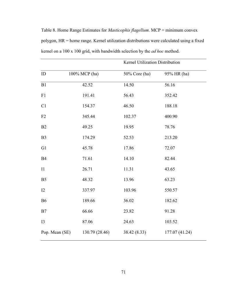
71

Table 8. Home Range Estimates for Masticophis flagellum. MCP = minimum convex

polygon, HR = home range. Kernel utilization distributions were calculated using a fixed

kernel on a 100 x 100 grid, with bandwidth selection by the ad hoc method.

Kernel Utilization Distribution

ID 100% MCP (ha) 50% Core (ha) 95% HR (ha)

B1 42.52 14.50 56.16

F1 191.41 56.43 352.42

C1 154.37 46.50 188.18

F2 345.44 102.37 400.90

B2 49.25 19.95 78.76

B3 174.29 52.53 213.20

G1 45.78 17.86 72.07

B4 71.61 14.10 82.44

I1 26.71 11.31 43.65

B5 48.32 13.96 63.23

I2 337.97 103.96 550.57

B6 189.66 36.02 182.62

B7 66.66 23.82 91.28

I3 87.06 24.63 103.52

Pop. Mean (SE) 130.79 (28.46) 38.42 (8.33) 177.07 (41.24)

72

Table 9. Masticophis flagellum Mean Daily Displacement. Raw = daily displacement calculated from all consecutive locations,

Independent = daily displacement calculated from all sequential displacements greater than three meters and excluding snakes in

ecdysis, digesting large meals, or otherwise inactive, Scrub = daily displacement calculated for biologically independent

consecutive locations within a patch of Florida scrub, and Other = daily displacement calculated for biologically independent

consecutive locations within all habitats except Florida scrub. The active season was considered all locations from March through

October, but movement of each individual occurred in every month.

ID Raw Independent Scrub Other Active Season

B1 119 (15) 136 (16) 103 (13) 113 (26) 150 (18)

F1 122 (25) 142 (28) 9 (3) 172 (54) 142 (28)

C1 149 (28) 175 (14) 127 (19) 197 (26) 194 (15)

F2 207 (21) 241 (24) 106 (53) 251 (33) 272 (27)

B2 88 (12) 97 (12) 84 (13) 91 (32) 105 (14)

B3 143 (11) 168 (13) 135 (14) 126 (44) 191 (15)

G1 93 (15) 109 (18) 94 (16) 57 (NA) 135 (22)

B4 134 (19) 169 (19) 56 (16) 225 (70) 188 (26)

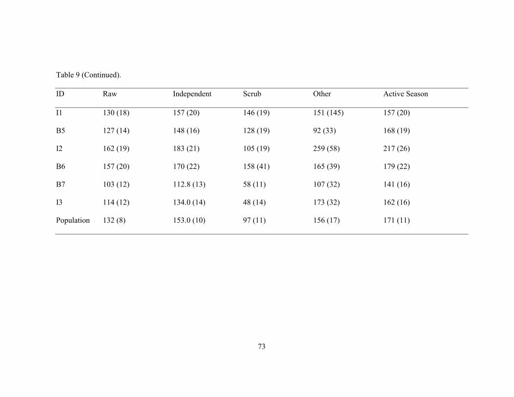
73


ID Raw Independent Scrub Other Active Season

I1 130 (18) 157 (20) 146 (19) 151 (145) 157 (20)

B5 127 (14) 148 (16) 128 (19) 92 (33) 168 (19)

I2 162 (19) 183 (21) 105 (19) 259 (58) 217 (26)

B6 157 (20) 170 (22) 158 (41) 165 (39) 179 (22)

B7 103 (12) 112.8 (13) 58 (11) 107 (32) 141 (16)

I3 114 (12) 134.0 (14) 48 (14) 173 (32) 162 (16)

Population 132 (8) 153.0 (10) 97 (11) 156 (17) 171 (11)

74

Table 10. Habitat Use and Availability for Masticophis flagellum. Availability (Avail) is the expressed as the percentage of each individual’s home range made up of each habitat. Use is the number

of locations (percentage of locations) in each habitat. Blanks indicate a habitat that was not available to the individual. For the study site, habitat availability is expressed as hectares (percentage of

total).

Marsh Swamp Cutthroat Flatwoods Sandhill Florida Scrub Pasture

ID Avail Use Avail Use Avail Use Avail Use Avail Use Avail Use Avail Use

B1 2.9 0 (0) 2.1 0 (0) 26.4 6 (7.0) 13.0 13 (15.1) 9.4 6 (7.0) 46.2 61 (70.9)

F1 4.9 0 (0) 0.4 0 (0) 24.0 1 (3.8) 36.5 9 (34.6) 6.9 12 (46.2) 27.3 4 (15.4)

C1 0.8 0 (0) 0.9 2 (1.1) 10.2 3 (1.6) 19.3 76 (41.1) 8.1 26 (14.1) 60.1 78 (42.2)

F2 7.1 0 (0) 2.8 0 (0) 19.7 13 (7.4) 42.0 78 (44.6) 0.7 1 (0.6) 26.2 83 (47.4)

B2 0.1 0 (0) 3.6 0 (0) 19.3 4 (5.6) 15.8 2 (2.8) 11.5 22 (30.6) 49.7 44 (61.1)

B3 1.9 0 (0) 10.1 0 (0) 10.8 0 (0) 33.0 40 (21.1) 5.6 7 (3.7) 38.6 143 (75.3)

G1 6.3 0 (0) 4.4 0 (0) 0.6 1 (1.8) 20.8 3 (5.4) 21.0 9 (16.1) 46.8 43 (76.8)

B4 8.0 0 (0) 11.1 0 (0) 55.0 19 (27.1) 26.0 51 (72.9)

I1 4.2 0 (0) 22.0 7 (11.7) 73.6 53 (88.3)

B5 2.2 0 (0) 10.4 1 (1.0) 18.9 16 (15.4) 10.5 12 (11.5) 58.1 75 (72.1

I2 41.5 0 (0) 18.3 0 (0) 9.8 32 (30.5) 1.3 3 (2.9) 29.2 70 (66.7)

B6 17.5 0 (0) 24.3 5 (7.0) 17.3 28 (39.4) 3.2 1 (1.4) 37.5 37 (52.1)

B7 10.0 0 (0) 8.6 3 (3.1) 52.4 27 (28.1) 29.0 66 (68.8)

I3 0.3 0 (0) 0.5 0 (0) 5.4 4 (4.3) 69.7 39 (41.9) 9.6 50 (53.8) 14.6 0 (0)

Study Site 30.6 (2.3) 230.3 (17.5) 289.1 (21.9) 368.0 (27.9) 25.5 (1.9) 274.2 (20.8) 101.9 (7.7

75

Table 11. Manly’s Standardized Selection Ratios (B) for Habitats Selected by

Masticophis flagellum. Habitats are listed in decreasing order of habitat selection.

Superscripts indicate statistically significant differences in selection between habitats.

Home Range Selection Habitat Selection

Habitat B P B P

Florida Scrub 0.23a 0.0038 0.59a <0.001

Flatwoods 0.13bc 0.59 0.29b 0.022

Sandhill 0.32ab 0.083 0.12bc 0.677

Cutthroat 0.077cde 0.0028 0.035c <0.001

Pasture 0.047cde 0.046 0.022cd 0.157

Swamp 0.042de 0.0023 0.003d <0.001

Marsh 0.15abcd 0.50 0.00d <0.00

76

Table 12. Summary of Models Evaluated for Habitat Selection by Masticophis flagellum. K = number of parameters in the model.

Models are listed in order of decreasing support.

Model Deviance K AICc ΔAICc AICc Wt.

Selection varies among individuals 0 98 428 0 1.00

Constant selection of habitat 329 20 586 159 <<0.001

Selection varies with sex 476 14 722 294 <<0.001

Selection varies with size 486 14 731 303 <<0.001

No selection of habitat 2552 14 2797 2369 0.00

77

Table 13. Florida Scrub Patch Use and Availability for M. flagellum. Availability (Avail) is the expressed as the percentage of each

individual’s home range made up of each Florida scrub patch. Use is the number of locations (percentage of locations) in each

patch. Blanks indicate patches that were not available to the individual.

A B C D E

ID Avail Use Avail Use Avail Use Avail Use Avail Use

B1 52.2 65 (98.5)

C1 2.6 3 (2.9) 64.9 101 (97.1) 0.8 0 (0)

F2 3.6 8 (14.8) 10.5 16 (29.6) 0.3 0 (0) 0.3 1 (1.9) 0.6 7 (13.0)

B2 59.8 63 (98.4)

B3 7.1 14 (9.5) 34.3 127 (86.4)

B4 5.6 11 (21.6)

B5 2.4 2 (2.3) 65.8 82 (94.3) 0.3 3 (3.4)

I2 19.9 23 (69.7)

B7 12.8 22 (33.3) 10.8 25 (37.9) 0.9 1 (1.5)

78


F G H I

ID Avail Use Avail Use Avail Use Avail Use

B1 3.4 1 (1.5)

C1

F2 0.8 10 (18.5) 0.7 4 (7.4) 3.8 8 (14.8)

B2 1.3 1 (1.6)

B3 2.8 6 (4.1)

B4 3.1 7 (13.7) 16.6 33 (64.7)

B5

I2 6.0 10 (30.3)

B7 3.5 17 (25.8) 1.0 1 (1.5)

79

Table 14. POPAN Jolly-Seber Abundance Estimates for Lizard and Mammalian Prey in Each Sampled Patch of Florida Scrub.

Abundance estimates are per trap array over the entire study period (March 2004 – June 2006). Estimates were derived from the

best-fit model indicated in the table. Abundance estimates are presented as mean (standard error). Estimates used in the

examination of the effect of prey abundance on patch selection by M. flagellum were mean monthly abundance for the tracking

period of each snake, and were lower than the study period estimates presented here. AICc wt. = relative support of model

compared with other models evaluated for each species, p = capture probability, Φ = survival probability, pent = probability of

entry (birth and immigration). • = constant parameter value, t = time-varying parameter, g+t = parameter varied over time in a

parallel manner for each group.

Patch Abundance Estimate

Prey Species Model AICc wt. A B C D

Anolis carolinensis p•Φ•pent• >0.99 21.0 (8.5) 31.7 (10.9) 42.5 (13.3) 17.4 (7.6)

Aspidoscelis sexlineata ptΦ•pentg+t 0.98 67.7 (9.8) 85.7 (11.5) 92.0 (12.8) 90.4 (12.3)

Sceloporus woodi ptΦ•pent• 0.90 172.8 (18.9) 168.7 (18.6) 83.4 (12.2) 4.8 (2.9)

Peromyscus polionotus p•Φ•pentt >0.99 27.3 (3.9) 32.7 (4.9) 7.8 (1.1) 19.5 (2.8)

Podomys floridanus p•Φ•pentt >0.99 84.2 (12.2) 67.5 (10.4) 93.3 (13.1) 62.9 (10.0)

80


Patch Abundance Estimate

Prey Species E F G H I

Anolis carolinensis 49.7 (14.8) 46.1 (14.0) 60.4 (17.0) 49.7 (14.8) 22.8 (8.9)

Aspidoscelis sexlineata 135.9 (16.0) 110.2 (14.2) 236.9 (22.6) 179.3 (18.2) 57.9 (9.5)

Sceloporus woodi 2.0 (2.0) 156.5 (17.7) 0 (0) 75.2 (11.5) 122.7 (15.3)

Peromyscus polionotus 0 (0) 3.9 (0.6) 27.3 (3.9) 43.8 (7.3) 60.4 (9.8)

Podomys floridanus 132.9 (17.0) 117.7 (15.5) 93.3 (13.1) 59.9 (9.7) 70.5 (10.8)

81

Table 15. Summary of Models Evaluated for Florida Scrub Patch Selection by Masticophis flagellum. K = number of parameters in

model, Swoo Abund =Sceloporus woodi abundance, Liz Abund = lizard (Anolis carolinensis + Aspidoscelis sexlineata + S. woodi)

abundance, Mam Abund = mammal (Peromyscus polionotus + Podomys floridanus) abundance. Models with interactions allow

selection to vary by individual or characteristic; additive models demonstrate constant selection by individual or characteristic.

Models are listed in order of decreasing support.


Snake x Scrub 0 81 291 0 1.00

Snake + Scrub 462 17 615 324 <<0.001

Sex x Scrub 496 18 652 361 <<0.001

Size x Scrub 523 18 678 387 <<0.001

Snake x Swoo Abund 1072 18 1227 937 <<0.001

Snake + Swoo Abund 1222 10 1361 1070 <<0.001

Snake x (Liz Abund + Mam Abund) 1486 18 1659 1368 <<0.001

Snake x Mam Abund 1599 18 1754 1463 0.00

Snake + Liz Abund + Mam Abund 1689 27 1831 1540 0.00

82



Snake + Mam Abund 1702 10 1842 1551 0.00

Snake x Liz Abund 1755 18 1910 1619 0.00

No Selection 1813 9 1950 1659 0.00

Snake + Liz Abund 1811 11 1950 1659 0.00

Size x Mam Abund 1856 4 1984 1692 0.00

83

Table 16. Manly’s Standardized Selection Ratios (B) for Florida Scrub Patches Selected

by Masticophis flagellum. Patches are listed in decreasing order of selection. Superscripts

indicate statistically significant differences in selection between patches. * - Patch was

only available to one snake, so statistical significance of selection of this patch could not

be determined.

Patch B P

B 0.43a 0.0083

F 0.16b 0.33

H 0.13b 0.63

A 0.11b 0.66

G 0.064b 0.38

E 0.047b 0.45

I 0.045b 0.32

C 0.012b 0.023

D* 0.012 NA

84

Table 17. Home Range Sizes and Movement Distances of Masticophis flagellum at Different Locations. Numbers in the table

indicate mean (se). Mean Daily Displacement is the mean straight-line daily movement, which was determined by different field

and/or analytical techniques in each study. * - Home range size and mean daily displacement were calculated excluding the

individual tracked only through winter.

Study Location 100% MCP (ha) Mean Daily Displacement (m)

This study Central Florida 130.8 (28.5) 153 (10)

Secor, 1995 Mojave Desert 57.9 (13.2) 146 (13)

Dodd and Barichivich, 2007* North-central Florida 113.6 (38.5) 229 (47)

Johnson et al., 2007 Eastern Texas 70.4 (83.8) 93 (NA)

85

Figure 5. Map of the Study Site within the Lake Arbuckle Tract of Lake Wales Ridge

State Forest in Central Florida, USA. The 100% minimum convex polygon containing all

snake locations is outlined by the dashed black line, and focal patches of scrub are

outlined and labeled in solid black.

Figure 6. Masticophis flagellum Net Squared Displacement Versus Random Walk

Expectations. Observed squared displacement is represented by the dashed line, expected

squared displacement is represented by the solid black line, and the 95% confidence

interval is represented by dotted lines. The observed squared displacement generally lies

along the x-axis. Scales on the x-axis are constant in columns; scales on the y-axis are

constant in rows.

86

Figure 7. Masticophis flagellum 100% Minimum Convex Polygon Home Ranges.

Females are indicated by solid lines, males are indicated by dotted lines.

87

Figure 8. Mosaicplot of the Frequency of Behaviors within Habitats. Habitats with fewer

than 20 observations were not included in the plot. The width of bars indicates the

proportion of observations within each habitat, the height of each subdivision indicates

the proportion of each behavior within each habitat.

88

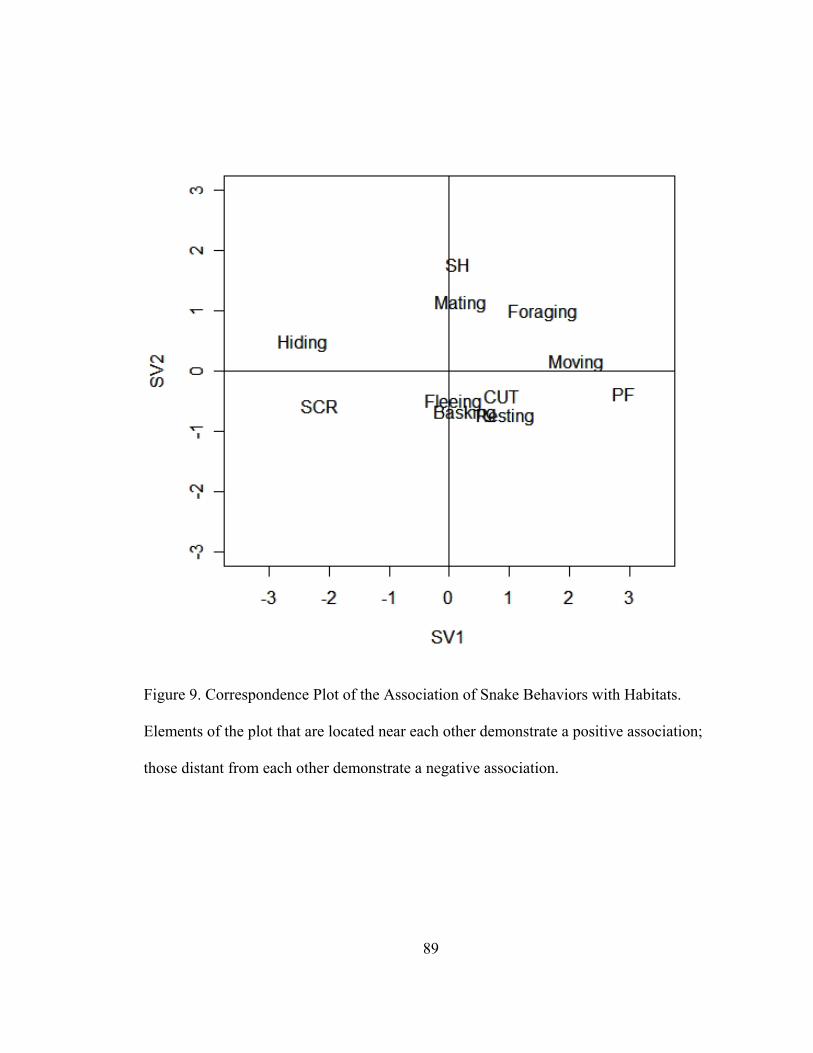
Figure 9. Correspondence Plot of the Association of Snake Behaviors with Habitats.

Elements of the plot that are located near each other demonstrate a positive association;

those distant from each other demonstrate a negative association.

89

90

A Greater Abundance of Snakes Results in Lower Survival Rates of Florida Scrub

Lizard (Sceloporus woodi) Populations

Although broad variation in the demography of lizards in the genus Sceloporus

occurs, the mechanisms leading to this variability are unresolved (Tinkle and Dunham

1986). For instance, phylogenetic, geographic, and habitat differences in demographic

parameters exist among populations of Sceloporus undulatus (Ferguson et al. 1980), but

the source of these differences is unclear. Density-dependent predation and density-

independent stochastic environmental factors affect temporal differences in survivorship

and fecundity in a Kansas population of S. undulatus (Ferguson et al. 1980). Predation

has been repeatedly suggested as a determinant of the local life histories of populations of

S. undulatus (Crenshaw 1955, Tinkle and Dunham 1986), but much of the evidence is

anecdotal.

The demography of Sceloporus woodi is a particularly interesting case study.

Sceloporus woodi has a very short lifespan, with a maximum recorded age of 27 months

(McCoy et al. 2004). Although it can be locally abundant, S. woodi is considered rare

because it occurs only in Florida, USA, and there it is precinctive to the rare and

fragmented Florida scrub habitat (Jackson 1973, McCoy and Mushinsky 1992).

Individuals of S. woodi disperse a maximum distance of 750 m, but dispersal movements

greater than 200 m are rare. Dispersal of S. woodi is restricted to an even greater extent

by the densely vegetated habitats that typically occur between patches of Florida scrub

91

(Hokit et al. 1999). These habitat and dispersal characteristics of S. woodi, together with

the natural and anthropogenic fragmentation of Florida scrub (McCoy and Mushinsky

1994), contribute to the existence of this species as metapopulations (Hokit et al. 2001).

The mechanisms regulating S. woodi metapopulations and local populations

remain unclear. Reduced survival of S. woodi in smaller patches of scrub occurs, but the

mechanism for this effect is uncertain (Hokit and Branch 2003b), although predation has

been suggested (McCoy et al. 2004). To examine the roles of patch size and predation

pressure on the abundance and survival rates of S. woodi, I studied temporal and spatial

variation in these parameters within a single metapopulation of S. woodi while

quantifying the relative abundance of co-occurring saurophagous snakes. I predicted that

abundance and survival rates of S. woodi would vary temporally with its life cycle, and

spatially as a function of patch size and snake abundance. I found that the abundance of

S. woodi exhibited both temporal and spatial variation, and survival rates of this lizard

were most strongly affected by the relative abundance of snakes.


Study Site

Research was conducted at the Lake Arbuckle tract of the Lake Wales Ridge


Longitude). The site consists of a series of patches of xeric Florida scrub habitat and

wetlands in a matrix of more densely vegetated pine flatwoods habitat. All sampling

occurred in nine neighboring patches of Florida scrub habitat ranging in size from 1.5-

92

170 ha (Fig. 10). Sampled patches were similar in vegetation composition and structure,

and each was dominated by a low (0.5-1.5 m) midstory of shrub oak (Quercus spp.),

scrub palm (Sabal etonia), and saw palmetto (Serenoa repens). Canopy cover in the

sampled locations was typically less than 10%, and primarily consisted of slash pine

(Pinus elliottii). Groundcover in sampled locations was primarily bare sand with less than

50 percent leaf litter and little herbaceous vegetation.

Field Methods

Sceloporus woodi was sampled using 13 trap arrays (see below) installed in the

patches of Florida scrub habitat. One trap array was installed in each scrub, with the

exception that two trap arrays were installed in scrub I, and four trap arrays were installed

in scrub B to account for potentially greater heterogeneity in density and survival rate in

larger patches (Fig. 10). Trap arrays consisted of a central box trap with a funnel on each

face and four 7.6 m drift fences constructed of 50.8 cm aluminum flashing projecting

from each face of the box trap (Burgdorf et al. 2005). A single-ended funnel trap

constructed of 6.35 mm hardware cloth was placed on each side of the distal end of each

drift fence, and a 7.6-L bucket was placed at the center of both sides of each drift fence

for a total of 17 traps per array (Fig. 11). All traps were shaded with Masonite and

provided with a moist sponge to prevent desiccation and overheating of trapped

individuals. Trap arrays were opened and checked daily for seven consecutive days

(secondary period), then closed for 21 consecutive days (primary period) as part of a

robust capture-recapture design (Pollock 1982). Sampling occurred from March 2004 –

June 2006 for a total of 20 primary periods. Traps were closed from December 2004 –

93

February 2005 and again from November 2005 – March 2006 to avoid small mammal

mortality caused by cold overnight temperatures. Each day traps were checked, the

maximum, minimum, and current temperature (°C) were measured with a max/min

thermometer, and amount of precipitation (mm) was measured with a rain gauge at trap

array A1 (Fig. 1). All captured S. woodi were sexed, measured for snout-vent length

(SVL) and total length (TL) to the nearest mm, weighed to the nearest 0.1 g, given a

unique identifying mark by toe clipping (Waichman 1992), and released a few meters

outside the trap array.

Analytical Methods

Capture-recapture data for S. woodi were analyzed using the ad hoc robust design

(Pollock, 1982) with Program MARK 4.3 (White, 2006). Abundance estimates were

calculated for each secondary period at each trap array using Huggins’ closed population

models (Chao and Huggins 2005). Daily capture probabilities were assumed to be the

same at all trap arrays, which were identical, were placed in scrub habitat with very

similar structural attributes, and were close enough to one another that each array

experienced similar environmental conditions. Capture and recapture probabilities also

were considered equal for two a priori reasons. First, the traps were not baited, so lizards

were unlikely to exhibit a “trap-happy” response. Second, lizards that were trapped did

not appear stressed relative to lizards found outside the traps, and it is unlikely that they

learned to intentionally avoid traps. Huggins’ closed population models that I evaluated

were constant (re)capture probabilities (p.), individual heterogeneity in (re)capture

probabilities (two mixture model; phet), time-specific (re)capture probabilities (pt), and

94

combined time and heterogeneity effects (phet*t). In addition to these basic models, daily

mean temperature (ptemp) and rainfall (prain) were used as environmental covariates; the

effect of these environmental variables on individual heterogeneity (phet*temp and phet*rain)

also was evaluated. Sex (psex) and SVL (pSVL) were individual characteristics used in an

attempt to explain sources of heterogeneity in (re)capture probabilities and improve the

estimation efficiency of lizard abundance (Chao and Huggins 2005). Two-way interactive

and additive models between individual covariates and time (psex*t, psex+t, pSVL*t, and

pSVL+t) or temperature (psex*temp, psex+temp, pSVL*temp, and pSVL+temp) also were evaluated.

Thus, up to 18 models were considered for each secondary period. All models with

covariates were analyzed using the logit link function, which maps the probability of a

binary response variable (in this case, captured or not captured) from [0,1] to [-∞,+∞]

(Cooch and White 2007). If no rain fell during a secondary period, all models that

included rainfall were eliminated from the analysis. Additionally, models that contained

more parameters than the number of individual lizards captured during that week also

were not considered for analysis because data for these weeks were too sparse to estimate

all parameters of these models. Thus, as few as 12 models were evaluated for some

secondary periods.

Survival rates were determined using Cormack-Jolly-Seber (CJS) models

(Nichols 2005) in Program MARK 4.3 (White, 2006). Secondary period capture histories

were combined to construct primary period capture histories. My model set was

constructed using a two step procedure. Recapture probabilities in the first step were

modeled as constant (p.), time-varying (pt), or as a linear function of mean secondary

period temperature (ptemp), rainfall (prain), or breeding season (March, April, and May) vs.

95

non-breeding season (all other secondary periods; pbreeding). Recapture probabilities were

assumed to be the same in all patches of scrub habitat. Survival rates in the first step were

modeled as constant (Φ.), time-varying (Φt), and as a function of the patch in which the

individual was captured (Φscrub). Interactive and additive models (Φscrub*t and Φscrub+t,

respectively) also were evaluated. Survival rate and recapture probability were included

in all possible combinations, resulting in an initial set of 25 models. I used the bootstrap

procedure to evaluate overdispersion (the presence of excess variation in the data not

explained by the binomial model) for my global model (Φscrub*tpt), and based my

adjustment of the variance inflation factor (ĉ = 1.125) upon the ratio of the observed

deviance to the mean of the bootstrapped deviances (Cooch and White 2006). Because

only models Φ.pt, Φtpbreeding, and Φ.pbreeding received support from my data, I only used pt

and pbreeding in step two of my model development procedure.

The second step in defining my CJS model set was to build models that examined

the importance of snake abundance and patch area in affecting the survival rates of S.

woodi. The relative abundance of snakes was determined as the number of saurophagous

snakes trapped in each patch, divided by the number of trap arrays in that patch.

Saurophagous snake species at my site included Coluber constrictor, Elaphe guttata,

Lampropeltis triangulum, Masticophis flagellum, and Micrurus fulvius. Scrub area was

determined by walking the boundary of each patch with a GPS receiver, and using the

area calculated from the differentially-corrected rover file (Trimble® GPS Pathfinder

Office 2.90). Snake abundance and patch area were then used as spatial covariates in CJS

models to constrain the effect of scrub on survival rate to be a linear function of snake

relative abundance (Φsnake) or scrub area (Φarea). Interactive and additive models of snake

96

abundance and patch area with time (Φsnake*t, Φsnake+t, Φarea*t, and Φarea+t) and each other

(Φsnake*area, Φsnake+area) also were evaluated, resulting in a final set of 41 models. All

models with covariates were analyzed using the logit link function (Cooch and White

2007).

Models for all analyses were evaluated for parsimony using Akaike’s Information

Criterion adjusted for small sample sizes and overdispersion (QAICc). If more than one

model had a ΔQAICc value less than six (relative likelihood > 5%), parameters were

estimated using model averaging to account for uncertainty in model selection (Burnham

and Anderson 2002). The relative importance of variables (w+) was determined by

calculating the sum of the Akaike weights for all models containing each variable of

interest. The relative importance of variables is dependent upon the set of models

evaluated, but does not necessarily depend upon which particular model is most

parsimonious (Burnham and Anderson 2002).

RESULTS

I captured a total of 503 S. woodi individuals 878 times, and 417 individual

saurophagous snakes also were captured. Uncertainty in abundance estimates was usually

greater than the variation of these estimates in space and time (Fig. 12). No single model

was identified in the analysis as the most parsimonious explanation for any secondary

period. Indeed, the important variable(s) for determining (re)capture probabilities (an

index of lizard activity) was different from month to month (Table 18). Patch area did not

affect the density of S. woodi per trap array nor the variation in monthly abundance

estimates (Fig. 12).

97

The CJS confidence set included 12 models (Table 19; arranged from greatest to

least support). Models with time-varying recapture probabilities received the greatest

support from the data (w+ = 0.684); models including the effects of breeding activity on

recapture probability also were supported, but less strongly so (w+ = 0.316). Recapture

probability was greatest in the spring of each year and declined through the summer (Fig.

13). Survival rate was relatively constant over time, and estimates of the probability of an

individual surviving a four-week primary period ranged from 0.7 – 0.8 (Fig. 14). The

most important characteristics for determining survival rates were snake relative

abundance and patch area (Table 20).

DISCUSSION

The abundance of S. woodi varied over space and time, but scrub area did not

appear to affect density estimates. The factors affecting the daily (re)capture probability

of S. woodi individuals varied substantially among secondary periods. Usually, the sex of

an individual did not matter for determining (re)capture probability. The importance of a

particular factor likely depends upon the context of the sampling period with regard to the

environment, lizard phenology, or size and/or sex structure of the population. For

example, temperature may have a greater effect on lizard activity when temperatures are

more extreme or variable, and rainfall may more influential in very dry periods. Snout-

vent length might change in importance as the size structure of the population changes,

particularly if different size classes differ in activity level or susceptibility to trapping.

Sex might be more important during breeding or oviposition than at other periods. The

large proportion (65%) of secondary periods for which environmental or individual

98

covariates were of great importance indicates that the use of Huggins’ closed models is

an appropriate and desirable method of accounting for temporal and individual behavioral

heterogeneity when estimating the abundance of lizards, particularly because these

models can incorporate individual covariates.

My results indicated that S. woodi survival rates exhibited greater variation

between patches of scrub than they did over time. In particular, the relative abundance of

snakes had a larger effect on survival rate than any other measured characteristic. The

most obvious explanation for this negative effect is snake predation. Indeed, the two

snakes most frequently encountered on this site were Coluber constrictor and

Masticophis flagellum, which both consume S. woodi in proportion to its abundance

(Halstead et al. In review). In addition to predation, high numbers of snakes could alter

the behavior of S. woodi, resulting in greater risk of mortality from other causes,

including alteration of competitive interactions and decreased energy intake (Werner

1991, Lima 1998). Predation, particularly by snakes, is an important mortality factor for

Sceloporus spp. (Crenshaw 1955, Ferguson et al. 1980, McCoy et al. 2004), but has not

previously been quantified.

In contrast to the effects of snake abundance, patch area had a positive effect on

the survival rate of S. woodi. The positive effects of area were independent of the effect

of snake abundance. Models including interactive effects of snakes and area had less

support than additive models or models with each factor considered in isolation.

Therefore, the increase in survival rate with increasing patch area is not solely caused by

greater predation rates by snakes in smaller patches. Possibly, predation rates by avian or

mammalian predators are greater in smaller patches of scrub (Hokit and Branch 2003b).

99

The positive effect of patch area on the survival rate of S. woodi also could be caused by

many other factors, including lower abundance and changes in demographic rates

associated with small populations (see Hokit and Branch, 2003a).

The best-fit model in my model set indicated constant survival rates for S. woodi.

The fit of this model to the data is almost certainly a consequence of low statistical

power. Recapture probabilities of S. woodi were low, and my sample size was limited to

nine patches of Florida scrub, of which only six contained viable S. woodi populations.

Constant survival rates across patches and over time are unlikely to be a realistic

description of S. woodi survival, but rather a reflection of the limitations of my sample

size and sampling methods. In exploratory ecological studies such as this one, the cost of

a type II error is as great as (or greater than) the cost of a type I error (Shrader-Frechette

and McCoy 1993). Thus, my conclusion that the abundance of saurophagous snakes

affects survival rates of S. woodi warrants additional study of the role of snakes in the

local and metapopulation dynamics of S. woodi.

In conclusion, my results provide quantitative evidence that the local abundance

of saurophagous snakes is inversely related to survival rates of local populations of S.

woodi. The demography of S. woodi could be particularly affected by abundant, actively

foraging predators such as C. constrictor and M. flagellum. Optimal patch use by these

wide-ranging predators may result in stabilizing density-dependent mortality of local

populations of S. woodi. Whether such an adaptive response by these snake species to

prey densities occurs is currently under investigation.

Table 18. Relative Importance (w+) of Environmental and Individual Characteristics for Determining the Daily (Re)capture Rate of

Sceloporus woodi. Numbers in Bold indicate the variable(s) with the greatest support from the data for each secondary period. * -

models for which (re)capture probability did not vary. † - w+ (number of models). ‡ - Secondary period for which mixture models

for unexplained individual heterogeneity in (re)capture probability were most parsimonious.

Variable

Secondary Period Constant* Time Temp. Rain SVL Sex

March 04 0.003 (1)† 0.992 (5) 0.002 (5) NA 0.189 (5) 0.280 (5)

April 04 0.041 (1) 0.016 (5) 0.841 (5) 0.050 (1) 0.222 (5) 0.379 (5)

May 04 0.068 (1) 0.011 (5) 0.326 (5) 0.036 (1) 0.608 (5) 0.261 (5)

June 04 0.050 (1) 0.472 (5) 0.340 (4) 0.052 (1) 0.310 (4) 0.485 (5)

July 04 0.153 (1) 0.648 (3) 0.086 (3) 0.057 (1) 0.709 (5) NA

August 04 0.070 (1) 0.194 (3) 0.511 (3) 0.028 (1) 0.750 (5) NA

September 04 0.149 (1) 0.411 (5) 0.184 (5) 0.076 (1) 0.153 (5) 0.363 (5)

October 04 0.055 (1) 0.002 (3) 0.893 (5) 0.029 (1) 0.039 (5) 0.841 (2)

November 04 0.330 (1) 0.011 (2) 0.334 (3) 0.199 (1) 0.277 (4) NA

100

101


Variable

Secondary Period Constant* Time Temp. Rain SVL Sex

March 05‡ 0.057 (1) 0.007 (1) 0.006 (1) 0.897 (1) NA NA

April 06 0.014 (1) 0.809 (5) 0.064 (5) 0.006 (1) 0.747 (5) 0.144 (5)

April 05 0.098 (1) 0.014 (5) 0.260 (5) 0.554 (1) 0.102 (5) 0.107 (5)

May 05 0.098 (1) 0.076 (5) 0.495 (5) 0.250 (1) 0.306 (5) 0.155 (5)

May 06 0.110 (1) 0.186 (5) 0.618 (5) NA 0.237 (5) 0.258 (5)

August 05 0.184 (1) 0.041 (5) 0.552 (5) 0.067 (1) 0.166 (5) 0.387 (5)

June 05 <0.001 (1) 0.796 (5) 0.036 (5) 0.168 (1) 0.232 (5) 0.197 (5)

October 05 0.088 (1) 0.694 (5) 0.111 (5) 0.033 (1) 0.493 (5) 0.132 (5)

July 05 0.331 (1) 0.029 (5) 0.260 (5) 0.128 (1) 0.193 (5) 0.203 (5)

September 05 0.220 (1) 0.023 (5) 0.471 (5) 0.127 (1) 0.279 (5) 0.179 (5)

June 06 0.336 (1) 0.004 (5) 0.280 (5) 0.129 (1) 0.193 (5) 0.218 (5)

102

Table 19. Support of Cormack-Jolly-Seber Models for Sceloporus woodi Populations.

Models are listed in decreasing order of support, and only those models with a relative

likelihood greater than 0.05 are included in the table. Rel. Likelihood = likelihood of the

model relative to the most parsimonious model. K = number of parameters in model.

ĉ = 1.125.

Model Rel. Likelihood K QAICc Δ QAICc QAICc Wt.

Φ.pt 1.000 20 1072.494 0.000 0.222

Φsnakept 0.697 21 1073.216 0.722 0.155

Φarea+snakept 0.679 22 1073.269 0.775 0.151

Φareapt 0.435 21 1074.161 1.667 0.097

Φtpbreeding 0.419 21 1074.235 1.741 0.093

Φsnake+tpbreeding 0.310 22 1074.837 2.343 0.069

Φarea*snakept 0.251 23 1075.258 2.764 0.056

Φ.pbreeding 0.164 3 1076.109 3.615 0.036

Φarea+tpbreeding 0.158 22 1076.190 3.696 0.035

Φarea+snakepbreeding 0.127 5 1076.618 4.124 0.028

Φsnakepbreeding 0.117 4 1076.792 4.298 0.026

Φareapbreeding 0.074 4 1077.713 5.219 0.016

103

Table 20. Relative Importance (w+) of Variables for Determining the Survival Rate of

Sceloporus woodi Populations. * - + indicates a variable that increases survival rate,

- indicates a variable that decreases survival rate.

Variable No. Models w+ Direction of Influence*

Snake Relative Abundance 10 0.496 -

Scrub Area 10 0.394 +

Constant Survival Rate 2 0.259 NA

Time 14 0.198 NA

Patch of Scrub 6 0.004 NA

Figure 10. Map of the Study Site within the Lake Arbuckle Tract of Lake Wales Ridge

State Forest in Central Florida. Individual patches of scrub are outlined in solid black,

and the location and identity of trap arrays within each scrub is indicated.

104

Figure 11. Schematic Diagram Depicting the Layout of Each Trap Array. The central

square is a box trap. The horizontal and vertical solid lines represent four drift fences

ending at funnel traps represented by rectangles. The circles along the drift fences

represent pitfall traps. The triangles in the box and funnel traps indicate the location of

funnels allowing entrance of animals into the traps.

105

Figure 12. Model-averaged Estimates of Abundance for Sceloporus woodi Populations at

Each Trap Array Grouped by Patch Size. (A) Trap arrays in scrub B (170 ha). (B) Trap

arrays in scrub I (40 ha). (C) Trap arrays in scrub A and scrub H (13 and 9 ha,

respectively). (D) Trap arrays in scrub C and scrub F (1.5 and 3.0 ha, respectively). Error

bars overlap for most trap arrays for most months, and have been omitted for clarity of

presentation.

106

Figure 13. Model-averaged Estimates of Recapture Probability for Each Secondary

Period for Sceloporus woodi Populations. Recapture rate was assumed equivalent for

each local population. Error bars indicate 95% confidence intervals.

107

Figure 14. Model-averaged Estimates of Survival Rate for Each Primary Period for

Sceloporus woodi Populations. Error bars indicate 95% confidence intervals.

108

109

Conclusion: The Predicted Effects of Snake Predation upon Sceloporus woodi

Populations

Perhaps the most fundamental question one must ask when examining the

population ecology of rare species is: What mechanisms drive the dynamics of this

population? The answer to this question is essential for informing conservation and

management practices. Superficially attempting to increase fecundity or survival rates

without addressing the root causes of decline will not aid in the recovery of populations.

Undoubtedly, the occurrence of Florida scrub-precinctive Sceloporus woodi (Florida

Scrub Lizard) has been reduced by the loss of scrub habitat (Jackson 1973, Myers 1990,

McCoy and Mushinsky 1992). The focus of my study was not on broad-scale questions

of occurrence, but rather was the importance of factors influencing the demography of S.

woodi in the remaining patches of Florida scrub habitat where this species persists.

Chapters 2-4 of this dissertation have endeavored to examine one specific hypothesis:

Snakes, particularly wide-ranging Masticophis flagellum (Coachwhip), have the potential

to regulate local populations of S. woodi.

A very important consideration when examining the consequences of predation

for prey populations is the dietary breadth of the predator (Ryall and Fahrig 2006). I

found that both M. flagellum and the closely related, but more abundant, Coluber

constrictor (Racer) prey upon S. woodi. Masticophis flagellum specializes upon lizards

and mammals, but consumes prey opportunistically within these categories. Coluber

110

constrictor is a generalist predator of anurans, lizards, and mammals, but within the

amphibian category selects certain species upon which to forage. Both predators consume

S. woodi in proportion to its availability at fine temporal and spatial scales. Because

neither predator is dependent solely upon S. woodi for growth and reproduction, the

impact of these snake species upon S. woodi should be consistent with models that

consider a generalist predator.

One of the most basic and well-supported observations of predator-prey

interactions is that generalist predators, unlike specialists, do not depend upon a single

prey species to persist or increase in abundance. Thus, the numerical response of M.

flagellum is independent of the abundance of S. woodi. The impacts of M. flagellum upon

S. woodi populations will depend, however, upon the functional response that best

describes this interaction. Generalist predators can exhibit one of several functional

responses. One of the most widely recognized functional responses of generalist

predators is the Holling type III functional response (Murdoch 1969). The type III

functional response is sigmoid in shape, and suggests that consumption of prey

exaggerates differences in the availability of different prey species (Murdoch 1969).

Consumption of prey in proportion to their availability does not imply switching behavior

and is not consistent with a type III functional response. Rather, in a type III functional

response, a species at low relative densities is not consumed, but at high relative

densities, it is nearly always consumed (Murdoch 1969). The type III functional response

can result from a number of mechanisms, including prey residing in different habitats, the

formation of a search image, preference for recently consumed prey, and training that

increases prey capture probability (but not solely prey handling time (Murdoch 1969,

111

Oaten and Murdoch 1975, Murdoch 1977, McNair 1980)). Any or all of these

mechanisms may occur in the M. flagellum:S. woodi system, but the first is likely only

for a few alternative prey species, such as Sigmodon hispidus (Cotton Rat). Regardless of

the mechanism underlying the type III functional response, it tends to be stabilizing (by

reducing the amplitude of limit cycles and therefore increasing the persistence of the

predator-prey interaction) because prey species occurring at low abundances are excluded

from the predator’s diet. Therefore, rare prey experience little predation and their

population sizes are allowed to recover.

Another major class of generalist predation models does not make explicit

reference to the functional response, except that it is not type III. These models involve

incidental predation, which is defined as consumption of prey discovered while searching

for other prey, but which do not affect predator behavior (Vickery et al. 1992). Incidental

predation has little to no impact on the predator population, but it can have a large impact

upon rare prey populations. In these models, predators do not switch to alternative prey,

but rather consume incidental prey whenever it is encountered. In contrast to the

stabilizing effects of switching predators, incidental predation results in apparent

competition (Holt and Lawton 1994), which can lead to the extirpation or extinction of

rare prey. Apparent competition can result from a predator’s numerical response

(predator abundance is a function of total prey density), functional response (predators

concentrate foraging effort at areas of highest total prey density), or aggregative

movement, but in all cases the predator’s primary prey and incidental prey must occur

together (Schmidt and Whelan 1998). Because the capture rate of incidental prey is a

function of the search time for the predator’s primary prey, greater abundance of total

112

prey will lead to greater predation pressure on the incidental prey (Schmidt and Whelan

1998). This density independence (with respect to the incidentally-consumed prey) tends

to destabilize the interaction, and in particular can decrease the expected time to

extinction for rare prey (Schmidt and Whelan 1998). Although M. flagellum almost

certainly actively searches for S. woodi, incidental predation upon S. woodi by M.

flagellum is likely under certain conditions in this system (see below). Incidental

predation models have been successfully applied to Procyon lotor (Raccoon) predation

upon bird nests (Schmidt and Whelan 1998, Schmidt et al. 2001) and Peromyscus

leucopus (White-footed Mouse) predation upon Lymantria dispar (Gypsy Moth) pupae

(Goodwin et al. 2005).

Incidental predation does not necessarily require the response of a predator to the

density of alternative prey. If predators select certain habitats or habitat features for

resting, hiding, basking, or reproducing, prey residing in these areas may be consumed

incidentally. For example, nest predation rates are higher near forest edges (Andren and

Angelstam 1988), but the use of forest edges by an ophidian nest predator, Elaphe

obsoleta (Black Rat Snake), is related to thermoregulation rather than prey abundance

(Blouin-Demers and Weatherhead 2001b, a, Carfagno et al. 2006, Carfagno and

Weatherhead 2006). Thus, incidental predation can have large impacts on prey

populations wherever predators congregate, regardless of the mechanism responsible for

increased predator abundance.

In addition to type III functional responses and incidental predation models,

several other models may have important implications for the consumption of S. woodi

by M. flagellum. In some cases, prey vulnerability may be more important than prey

113

abundance (Quinn and Cresswell 2004). For example, if it is difficult for M. flagellum to

catch Aspidoscelis sexlineata (Six-lined Racerunner) or subdue Podomys floridanus

(Florida Mouse), it may consume S. woodi because it is more vulnerable, rather than

more abundant, prey. Although prey vulnerability is not likely to be a factor if the

availability and predator success rate when hunting alternative prey is high (Quinn and

Cresswell 2004), decreased coupling of predator consumption with prey abundance is

likely to reduce abundances of vulnerable prey. A relatively recent functional response

model, the steady state satiation model, distinguishes prey handling from prey digestion

(Jeschke et al. 2002). This model may be particularly appropriate for snakes, because

handling prey necessarily prevents further prey capture, but the process of digestion

likely affects the probability that the predator searches for additional prey (Jeschke et al.

2002). Because M. flagellum is digestion-limited, rather than handling-limited, foraging

time is predicted to decrease with an increase in prey abundance (Jeschke et al. 2002).

Therefore, this model presents a potential mechanism for the observed prevalence of

resting behaviors by M. flagellum in scrub. In addition to its behavioral predictions, a

functional response based upon digestion limitation would likely reduce predation rates

when mammals (which are larger and have a lower surface area: volume ratio) are

consumed, which in turn would decrease predation rates upon S. woodi. Optimal diet

selection by M. flagellum based on energetic considerations is can increase the

persistence time of the predator-prey system, but suggests that the profitability of

alternative prey will have a strong influence on the persistence of the M. flagellum:S.

woodi interaction (Fryxell and Lundberg 1994). The more profitable the alternative prey,

the less stable the system and the shorter the persistence time (Fryxell and Lundberg

114

1994, van Baalen et al. 2001); this effect is similar to going from a type III functional

response at low alternative prey profitability to incidental predation at high alternative

prey profitability (van Baalen et al. 2001). Suboptimal switching and variation between

individuals in switching rules increase stability by decreasing the amplitude of

fluctuations in predator and prey abundances (Fryxell and Lundberg 1994, van Baalen et

al. 2001). Regardless of the conditions for stability, the presence of alternative prey

nearly always increases the persistence of the system, as long as they are included in the

diet (Fryxell and Lundberg 1994, van Baalen et al. 2001).

The consequence of generalist predation upon S. woodi by M. flagellum and C.

constrictor depends upon which of the above models most accurately describes the

predation process. The active foraging mode of these predators increases the likelihood

that they will regulate populations of their prey, particularly if prey are consumed

opportunistically (Rosenheim and Corbett 2003). My observation that neither predator

forages selectively upon lizard or mammal species (as opposed to these prey categories)

are counter-indicative of a type III functional response (Murdoch 1969); however, weak

preferences actually promote switching more readily than strong preferences (Murdoch

1969, Oaten and Murdoch 1975, McNair 1980). Therefore, it is nearly impossible to

evaluate the likelihood of a type III functional response based purely on field studies of

diet selection. Incidental predation likely describes the consumption of S. woodi by M.

flagellum in situations where local population densities of S. woodi are low, but the

prevalence of S. woodi in the diet of M. flagellum suggests that these predators likely

search for S. woodi or, at the very least, lizards. The functional response of M. flagellum

preying upon S. woodi is probably situation-specific, with stabilizing switching occurring

115

in cases where alternative prey occur in different habitats (Murdoch 1977) or when a

specific prey species is abundant enough to effectively “train” M. flagellum to search for

or capture it (Murdoch 1969, Oaten and Murdoch 1975, McNair 1980), and small so that

M. flagellum must forage frequently enough for positive reinforcement of the search

image or capture efficiency. In contrast, incidental predation could deplete S. woodi

populations in patches where S. woodi is rare, but several alternative prey species are

equitably distributed and prevent training (Vickery et al. 1992, Schmidt and Whelan

1998). Additional research is required to determine the appropriate functional

response(s), and the conditions under which it (they) occur in this system.

A particularly salient feature of the M. flagellum:S. woodi system is the patchy

distribution of scrub habitat on my site. This is an important characteristic because S.

woodi is restricted to Florida scrub (Jackson 1973, McCoy and Mushinsky 1992) and

disperses poorly through other habitats (Hokit et al. 1999). Masticophis flagellum also

positively selects Florida scrub habitat, but easily disperses through the habitat matrix.

Taken together, these features of my study system indicate that predator-prey

metapopulation models and models of patch choice by predators are appropriate for

examining the potential dynamics of this system. Although both species are scrub

specialists, I primarily consider models of patch choice by predators because of the very

different dispersal abilities of M. flagellum and S. woodi.

The ideal free distribution (IFD) describes the optimal distribution of predators

such that each predator maximizes its encounter rate with prey (Bernstein et al. 1988).

Thus, the IFD serves as a useful null model when examining the consequences of

predator behavioral decisions (Kacelnik et al. 1992). In addition to serving as a null

116

model, if a constant number of predators distribute themselves according to the IFD, prey

mortality is likely to be density-dependent and, therefore, the interaction will be stable,

with predation rates greater in patches with greater prey densities, causing asynchronous

prey cycles among the patches (Bernstein et al. 1988). Predators are likely to achieve the

IFD if they have a good estimate of global prey density, they are able to sample the

environment, they learn faster than they deplete prey, and the environmental grain is fine

relative to predator movements (Bernstein et al. 1988, 1991). In contrast, if the cost of

travel between patches is high (because of distance or mortality rates), if the predators

underestimate average global prey density, if prey depletion occurs faster than predator

learning, or if the environment is coarse-grained relative to predator movements, the

distribution of predators diverges from the IFD (Bernstein et al. 1988, 1991). The greater

the divergence from the IFD, the less stable the system with a constant number of

predators, because predation rates are not linked to prey density and can be high in

patches with low prey abundance (Bernstein et al. 1988, 1991). Over multiple predator

generations under the IFD, predator migration does not affect the stability properties (i.e.,

amplitude of population fluctuations) of the system (Bernstein et al. 1999). In contrast to

constant predator numbers, predator limitations that prevent the predators from achieving

the IFD promote system stability in the population dynamic model (Bernstein et al.

1999). In particular, lower migration rates increase the amount of asynchrony in the

system and promote persistence (Bernstein et al. 1999). The positive selection of scrub

patches with greater lizard abundance suggests that M. flagellum may be distributed

according to the IFD in relation to prey density, which is stabilizing over the short term

but destabilizing over the long term. The interplay between within-patch prey population

117

growth rates, predator movement rates, and the number of patches in the system makes

predicting long-term outcomes based on IFD models very uncertain (Bernstein et al.

1999).

Additional simulation models have examined the consequences of optimal patch

selection under different migration scenarios. Adaptive local dispersal, in which predators

leave a patch according to the marginal value theorem (Charnov 1976) and are distributed

only among neighboring patches, reduces the amplitude of prey population fluctuations

more than adaptive global or fixed dispersal rules (Fryxell and Lundberg 1993).

Imperfect leaving rules further reduce the amplitude of these fluctuations (Fryxell and

Lundberg 1993). Both adaptive local dispersal and imperfect leaving rules are likely

migration scenarios for real predators, and should lend stability to the M. flagellum:S.

woodi system. In addition to the effects of dispersal rules, the migration rate of predators

can be critical. Asynchrony (and therefore, stability) is enhanced when predator

migration rates are neither too great nor too small, and the greater the number of patches,

the more likely the occurrence of asynchronous dynamics (Jansen 2001). Yet another

model considers the effect of a predator’s time budget on movement, which results in

prey density-dependent migration of the predator (Huang and Diekmann 2001). In this

case, predators are reluctant to leave areas of high prey density, which reduces the

stabilizing effect of spatial heterogeneity (Huang and Diekmann 2001). Prey-density

dependent migration is arguably a more realistic description of predator movements than

diffusion, and demonstrates that caution may be warranted in examining the stabilizing

effects of spatial heterogeneity (Huang and Diekmann 2001).

118

The above models considered one type of prey, and may not be directly

applicable to the M. flagellum:S. woodi system. Despite this limitation, these models are

likely a useful description of the movement rules of M. flagellum in response to total prey

densities. Because the most common prey in the diet of M. flagellum occur in scrub, it

may be appropriate to model the dynamics of this system by substituting total prey

density for individual prey species’ density in the above models to model the movement

decisions and distribution of M. flagellum between patches, and model within-patch

dynamics using an appropriate model of generalist predation. Laboratory microcosm

studies involving apparent competition, a likely scenario in my system, have

demonstrated that the presence of an apparent competitor can reduce the persistence time

of the system (Bull et al. 2006). In particular, the importance of habitat (or landscape)

configuration for pairwise species interactions is greatly reduced in complex multispecies

interactions (Bull et al. 2006). Thus, the expected spatial stabilization of the M.

flagellum:S. woodi system may not occur in the presence of alternative prey.

Regardless of the functional response and movement rules employed by M.

flagellum, saurophagous snakes have a negative impact on within-patch survival rates of

S. woodi. Although my most parsimonious model included constant survival rates, rather

than any spatial or temporal variation in this parameter, the selection of this model is

most likely a reflection of insufficient data to detect the true spatial differences in

survival rates. Regardless of which model was selected as most parsimonious, however, I

found that snake abundance was more important for determining survival rate than patch

area, despite the latter variable being reported as the most influential variable for

differences in S. woodi survival rates in previous studies (Hokit and Branch 2003b).

119

Snakes can have strong negative impacts on prey populations (Savidge 1987, Rodda and

Fritts 1992, Calsbeek and Sinervo 2002), and my observation of reduced survival rates of

S. woodi in patches with abundant snake predators, taken with the documented

occurrence of S. woodi in snake diets, indicates that predation by snakes is sufficient to

reduce survival rates of S. woodi at the spatial scale of the patch.

The foraging and spatial ecology of M. flagellum, taken together with the role of

snake abundance in depressing survival rates of S. woodi local populations, leads to the

following predictions for this patchy predator-prey system. Despite the likely occurrence

of some incidental predation on S. woodi by M. flagellum, it is unlikely that S. woodi,

which is abundant both in many patches of scrub and in the diet of M. flagellum, is

generally an incidental prey item. Instead, M. flagellum likely switches among prey

categories, if not prey species, in some circumstances. For example, M. flagellum is

diurnal (Ernst and Barbour 1989) and likely preys upon rodents while they are

underground in burrows. Relatively few diurnally-active lizards (which constitute all

lizards found in the diet of M. flagellum at my site) would be expected to be found in

rodent burrows during the day, which would result in “training,” or switching behavior,

that stabilizes the system. Switching may be less common among the smaller size classes

of M. flagellum that are restricted to consuming lizards because of gape limitations, and

accounting for size structure in the M. flagellum population could result in a more

complex interaction. Another stabilizing mechanism that is likely to lead to persistence of

this system is suboptimal diet or patch choice (Fryxell and Lundberg 1993, 1994, van

Baalen et al. 2001). Masticophis flagellum is unlikely to perfectly estimate prey capture

rate or global prey availability, either in total or for any individual prey species. An

120

additional mechanism leading to increased persistence may be the influence of additional

trophic levels on the interaction of M. flagellum with its prey. In particular, if predators

control the population of M. flagellum, it may never reach great enough abundance to

threaten S. woodi populations with extirpation. The opportunity for diffuse interactions in

this food web containing dietary generalists would also increase the likelihood of

persistence (McCann et al. 1998). In summary, I expect that the dietary generalist and

habitat specialist M. flagellum is unlikely to extirpate S. woodi at more than a small local

patch scale.

The above predictions must be tempered with caution, however, because they

assume a static landscape of available Florida scrub. Habitat loss and fragmentation can

have drastic effects on the outcome of interspecific interactions (Ryall and Fahrig 2006).

In particular, this system is characterized by a precinctive prey organism preyed upon by

a dietary generalist, but habitat specialist, predator. Models of the effects of habitat loss

on metacommunity structure indicate several different potential effects of habitat loss in

this system. First, because it is a dietary generalist, M. flagellum likely causes some

degree of apparent competition among its shared prey. Generalist predators are favored

over specialist predators when habitat is destroyed (Swihart et al. 2001, Melian and

Bascompte 2002, Ryall and Fahrig 2006), but because it is a habitat specialist and most

of its prey are more abundant in scrub than in other habitats, dietary generality may not

be an advantage for M. flagellum. In particular, because it is a habitat specialist, loss of S.

woodi habitat is also loss of M. flagellum habitat. If M. flagellum depends upon scrub

habitat for persistence, as my habitat selection and home range analyses suggest, it is

likely to go extinct at a lower level of habitat loss than S. woodi (Swihart et al. 2001,

121

Melian and Bascompte 2002, Ryall and Fahrig 2006). Following the extinction of M.

flagellum, the dynamics of S. woodi are uncertain. If predation by M. flagellum is more

strongly limiting to S. woodi than resource abundance, S. woodi could increase in

abundance following the extinction of M. flagellum. (Bascompte and Sole 1998, Prakash

and de Roos 2002, Ryall and Fahrig 2006). The effects of habitat fragmentation per se is

expected to decrease the persistence of the system because M. flagellum has much greater

dispersal abilities than S. woodi, and can lower survivorship (and increase rates of

extinction) of S. woodi in patches of scrub (Ryall and Fahrig 2006). In summary, the

effects of habitat loss are likely to have a more adverse effect on populations of M.

flagellum than populations of S. woodi, but the opposite may be true for habitat

fragmentation per se.

Interestingly, in the face of habitat loss, C. constrictor is a more likely candidate

than M. flagellum to cause the extirpation and extinction of S. woodi. Three primary

mechanisms underlie this hypothesis. First, like M. flagellum, C. constrictor is a dietary

generalist. Unlike M. flagellum, however, C. constrictor consumes prey, particularly

amphibians, found in abundance in pine flatwoods and wetland habitats. The prey base of

C. constrictor is therefore independent of scrub habitat (Schmidt et al. 2001, Swihart et

al. 2001, Ryall and Fahrig 2006). Second, because it is found in a greater variety of

habitats (particularly pine flatwoods and disturbed areas), C. constrictor can persist at

high abundances despite the loss and fragmentation of scrub habitat (Schmidt and

Whelan 1998, Ryall and Fahrig 2006). A particular problem associated with this trait is

that incursions by C. constrictor into scrub from other habitats can cause an increase in

the critical patch size required for the establishment and persistence of S. woodi

122

populations, provided C. constrictor does not exhibit a type III functional response

(Cantrell et al. 2001). Finally, because C. constrictor is smaller and moves less than M.

flagellum, it may experience lower predation rates by visually-oriented predators (such as

raptors) and become locally abundant, resulting in strong top-down effects on S. woodi

populations (Rosenheim and Corbett 2003). Adaptable generalist species such as C.

constrictor are thus selected under conditions of anthropogenic habitat fragmentation and

disturbance, and can have strong negative effects on rare prey populations (Schmidt and

Whelan 1998, Ryall and Fahrig 2006).

In conclusion, the interaction of M. flagellum with S. woodi may be locally

unstable, but is likely to be persistent. The functional response of M. flagellum toward S.

woodi is likely to differ depending upon the relative abundances of prey in a patch, with

stabilizing type III functional responses common in large snakes that consume mammals

and when relatively few alternative prey species are numerically dominant. In contrast,

when S. woodi is rare and alternative prey more equitably distributed, training is less

likely to occur and destabilizing incidental predation more likely. The patchy distribution

of scrub is also likely to enhance persistence, particularly when a large number of patches

are distributed at varying distances from each other. Although M. flagellum is likely to be

extirpated at lower levels of habitat loss than S. woodi, the effects of anthropogenic

changes could have grave effects for S. woodi by increasing predation rates by dietary

and habitat generalist predators such as C. constrictor.

123

Literature Cited

Andheria, A. P., K. U. Karanth, and N. S. Kumar. 2007. Diet and prey profiles of three sympatric large carnivores in Bandipur Tiger Reserve, India. Journal of Zoology 273:169-175.

Andren, H., and P. Angelstam. 1988. Elevated predation rates as an edge effect in habitat islands: Experimental evidence. Ecology 69:544-547.

Andrews, K. M., and J. W. Gibbons. 2005. How do highways influence snake movement? Behavioral responses to roads and vehicles. Copeia 2005:772-782.

Arnold, S. J. 1993. Foraging theory and prey-size-predator-size relations in snakes. Pages 87-115 in R. A. Seigel and J. T. Collins, editors. Snakes: Ecology and Behavior. Blackburn Press, Caldwell, New Jersey, USA.

Ashton, R. E., Jr., and P. S. Ashton. 1981. Handbook of Reptiles and Amphibians of Florida. Part One: The Snakes. Windward Publishing, Inc., Miami, Florida.

Bascompte, J., and R. V. Sole. 1998. Effects of habitat destruction in a prey-predator metapopulation model. Journal of Theoretical Biology 195:383-393.

Bernstein, C., P. Auger, and J. C. Poggiale. 1999. Predator migration decisions, the ideal free distribution, and predator-prey dynamics. American Naturalist 153:267-281.

Bernstein, C., A. Kacelnik, and J. R. Krebs. 1988. Individual decisions and the distribution of predators in a patchy environment. Journal of Animal Ecology 57:1007-1026.

Bernstein, C., A. Kacelnik, and J. R. Krebs. 1991. Individual decisions and the distribution of predators in a patchy environment .2. The influence of travel costs and structure of the environment. Journal of Animal Ecology 60:205-225.

Blouin-Demers, G., and P. J. Weatherhead. 2001a. An experimental test of the link between foraging, habitat selection and thermoregulation in black rat snakes Elaphe obsoleta obsoleta. Journal of Animal Ecology 70:1006-1013.

Blouin-Demers, G., and P. J. Weatherhead. 2001b. Habitat use by black rat snakes (Elaphe obsoleta obsoleta) in fragmented forests. Ecology 82:2882-2896.

124

Bonnet, X., G. Naulleau, and R. Shine. 1999. The dangers of leaving home: dispersal and mortality in snakes. Biological Conservation 89:39-50.

Brodie, E. D., Jr., B. J. Ridenhour, and E. D. Brodie, III. 2002. The evolutionary response of predators to dangerous prey: Hotspots and coldspots in the geographic mosaic of coevolution between garter snakes and newts. Evolution 56:2067-2082.

Bull, J. C., N. J. Pickup, M. P. Hassell, and M. B. Bonsall. 2006. Habitat shape, metapopulation processes and the dynamics of multispecies predator-prey interactions. Journal of Animal Ecology 75:899-907.

Burgdorf, S. J., D. C. Rudolph, R. N. Connor, D. Saenz, and R. R. Schaefer. 2005. A successful trap design for capturing large terrestrial snakes. Herpetological Review 36:421-424.

Burnham, K. P., and D. R. Anderson. 2002. Model Selection and Multimodel Inference: A Practical Information-Theoretic Approach, 2nd edition. Springer, New York, New York.

Calenge, C. 2006. The package "adehabitat" for the R software: a tool for the analysis of space and habitat use by animals. Ecological Modelling 197:516-519.

Calsbeek, R., and B. Sinervo. 2002. An experimental test of the ideal despotic distribution. Journal of Animal Ecology 71:513-523.

Cantrell, R. S., C. Cosner, and W. F. Fagan. 2001. How predator incursions affect critical patch size: The role of the functional response. American Naturalist 158:368-375.

Carfagno, G. L. F., E. J. Heske, and P. J. Weatherhead. 2006. Does mammalian prey abundance explain forest-edge use by snakes? Ecoscience 13:293-297.

Carfagno, G. L. F., and P. J. Weatherhead. 2006. Intraspecific and interspecific variation in use of forest-edge habitat by snakes. Canadian Journal of Zoology-Revue Canadienne De Zoologie 84:1440-1452.

Carr, A. F. 1940. A contribution to the herpetology of Florida. University of Florida Publication, Biological Science Series 3:1-118.

Chao, A., and R. M. Huggins. 2005. Modern closed-population capture-recapture models. Pages 68-87 in S. C. Amstrup, T. L. McDonald, and B. F. J. Manly, editors. Handbook of Capture-Recapture Analysis. Princeton University Press, Princeton, New Jersey.

Charnov, E. L. 1976. Optimal foraging, the marginal value theorem. Theoretical Population Biology 9:129-136.

125

Conant, R., and J. T. Collins. 1998. A Field Guide to Reptiles and Amphibians: Eastern and Central North America, Third edition. Houghton Mifflin Company, Boston, Massachusetts.

Cooch, E., and G. C. White. 2006. Program Mark: A Gentle Introduction, 5th edition.

Cooch, E., and G. C. White. 2007. Program Mark: A Gentle Introduction, 6th edition.

Crenshaw, J. W., Jr. 1955. The life history of the southern spiny lizard, Sceloporus undulatus undulatus Latrielle. American Midland Naturalist 54:257-298.

Cundall, D. 1987. Functional morphology. Pages 106-140 in R. A. Seigel, J. T. Collins, and S. S. Novak, editors. Snakes: Ecology and Evolutionary Biology. Macmillan Publishing Co., New York, New York, USA.

Cundall, D., and H. W. Greene. 2000. Feeding in snakes. Pages 293-333 in K. Schwenk, editor. Feeding: Form, Function, and Evolution in Tetrapod Vertebrates. Academic Press, San Diego, California, USA.

Daly, J. W., C. W. Myers, and N. Whittaker. 1987. Further classification of skin alkaloids from neotropical poison frogs (Dendrobatidae), with a general survey of toxic/noxious substances in the Amphibia. Toxicon 25:1023-1095.

Desfilis, E., E. Font, and F. Guillen-Salazar. 2003. Stimulus control of predatory behavior by the Iberian wall lizard (Podarcis hispanica, Sauria, Lacertidae): Effects of familiarity with prey. Journal of Comparative Psychology 117:309-316.

Dodd, C. K., Jr., and W. J. Barichivich. 2007. Movements of large snakes (Drymarchon, Masticophis) in north-central Florida. Florida Scientist 70:83-94.

Downes, S. J. 2002. Size-dependent predation by snakes: selective foraging or differential prey vulnerability? Behavioral Ecology 13:551-560.

Ernst, C. H., and R. W. Barbour. 1989. Snakes of Eastern North America. George Mason University Press, Fairfax, Virginia.

Fahrig, L., and G. Merriam. 1994. Conservation of fragmented populations. Conservation Biology 8:50-59.

Ferguson, G. W., C. H. Bohlen, and H. P. Woolley. 1980. Sceloporus undulatus: Comparative life history and regulation of a Kansas population. Ecology 61:313-322.

Fitch, H. S. 1963. Natural history of the Racer Coluber constrictor. University of Kansas Publications Museum of Natural History 15:351-468.

126

Fitch, H. S., and H. W. Shirer. 1971. A radiotelemetric study of spatial relationships in some common snakes. Copeia 1971:118-128.

Ford, N. M., and G. M. Burghardt. 1993. Perceptual mechanisms and the behavioral ecology of snakes. Pages 117-164 in R. A. Seigel and J. T. Collins, editors. Snakes: Ecology and Behavior. Blackburn Press, Caldwell, New Jersey, USA.

Fryxell, J. M., and P. Lundberg. 1993. Optimal patch use and metapopulation dynamics. Evolutionary Ecology 7:379-393.

Fryxell, J. M., and P. Lundberg. 1994. Diet choice and predator-prey dynamics. Evolutionary Ecology 8:407-421.

Garton, J. D., and H. R. Mushinsky. 1978. Evidence for skin toxicity and unpalatability in Gastrophryne carolinensis Anura Microhylidae. American Zoologist 18:583.

Gillingham, J. C. 1987. Social behavior. Pages 184-209 in R. A. Seigel, J. T. Collins, and S. S. Novak, editors. Snakes: Ecology and Evolutionary Biology. Blackburn Press, Caldwell, New Jersey.

Goodwin, B. J., C. G. Jones, E. M. Schauber, and R. S. Ostfeld. 2005. Limited dispersal and heterogeneous predation risk synergistically enhance persistence of rare prey. Ecology 86:3139-3148.

Greenbaum, E. 2004. The influence of prey-scent stimuli on predatory behavior of the North American copperhead Agkistrodon contortrix (Serpentes : Viperidae). Behavioral Ecology 15:345-350.

Greenberg, C. H., D. G. Neary, and L. D. Harris. 1994. Effect of high-intensity wildfire and silvicultural treatments on reptile communities in sand-pine scrub. Conservation Biology 8:1047-1057.

Greene, H. W. 1983. Dietary correlates of the origin and radiation of snakes. American Zoologist 23:431-441.

Greene, H. W., and J. A. Rodriguez-Robles. 2003. Feeding ecology of the California Mountain Kingsnake, Lampropeltis zonata (Colubridae). Copeia 2003:308-314.

Gregory, P. T., and L. A. Isaac. 2004. Food habits of the Grass Snake in southeastern England: Is Natrix natrix a generalist predator? Journal of Herpetology 38:88-95.

Gregory, P. T., J. M. Macartney, and K. W. Larsen. 1987. Spatial patterns and movements. Pages 366-395 in R. A. Seigel, J. T. Collins, and S. S. Novak, editors. Snakes: Ecology and Evolutionary Biology. Macmillan Publishing Co., New York, New York, USA.

127

Halstead, B. J., H. R. Mushinsky, and E. D. McCoy. In review. Sympatric Masticophis flagellum and Coluber constrictor select vertebrate prey at different levels of taxonomy.

Hamilton, W. J., and J. A. Pollack. 1956. The food of some colubrid snakes from Fort-Benning, Georgia. Ecology 37:519-526.

Hartmann, P. P. 1993. Demography of a population of the Florida scrub lizard (Sceloporus woodi) in a sand pine scrub on the Lake Wales Ridge of central Florida. University of South Florida, Tampa, Florida.

Heard, G. W., D. Black, and P. Robertson. 2004. Habitat use by the inland carpet python (Morelia spilota metcalfei : Pythonidae): Seasonal relationships with habitat structure and prey distribution in a rural landscape. Austral Ecology 29:446-460.

Hokit, D. G., and L. C. Branch. 2003a. Associations between patch area and vital rates: Consequences for local and regional populations. Ecological Applications 13:1060-1068.

Hokit, D. G., and L. C. Branch. 2003b. Habitat patch size affects demographics of the Florida scrub lizard (Sceloporus woodi). Journal of Herpetology 37:257-265.

Hokit, D. G., B. M. Stith, and L. C. Branch. 1999. Effects of landscape structure in Florida scrub: A population perspective. Ecological Applications 9:124-134.

Hokit, D. G., B. M. Stith, and L. C. Branch. 2001. Comparison of two types of metapopulation models in real and artificial landscapes. Conservation Biology 15:1102-1113.

Holt, R. D., and J. H. Lawton. 1994. The ecological consequences of shared natural enemies. Annual Review of Ecology and Systematics 25:495-520.

Horn, H. S. 1966. Measurement of "overlap" in comparative ecological studies. American Naturalist 100:419-424.

Huang, Y. X., and O. Diekmann. 2001. Predator migration in response to prey density: What are the consequences? Journal of Mathematical Biology 43:561-581.

Hurlbert, S. H. 1978. The measurement of niche overlap and some relatives. Ecology 59:67-77.

Jackson, J. F. 1973. Distribution and population phenetics of the Florida scrub lizard, Sceloporus woodi. Copeia 1973:746-761.

Jackson, J. F., and S. R. Telford, Jr. 1974. Reproductive ecology of the Florida scrub lizard, Sceloporus woodi. Copeia 1974:689-694.

128

Jansen, V. A. A. 2001. The dynamics of two diffusively coupled predator-prey populations. Theoretical Population Biology 59:119-131.

Jeschke, J. M., M. Kopp, and R. Tollrian. 2002. Predator functional responses: Discriminating between handling and digesting prey. Ecological Monographs 72:95-112.

Johnson, D. H. 1980. The comparison of usage and availability measurements for evaluating resource preference. Ecology 61:65-71.

Johnson, R. W., R. R. Fleet, M. B. Keck, and D. C. Rudolph. 2007. Spatial ecology of the Coachwhip, Masticophis flagellum (Squamata : Colubridae), in eastern Texas. Southeastern Naturalist 6:111-124.

Joly, D. O., and B. R. Patterson. 2003. Use of selection indices to model the functional response of predators. Ecology 84:1635-1639.

Jones, K. B., and W. G. Whitford. 1989. Feeding-behavior of free-roaming Masticophis flagellum - an efficient ambush predator. Southwestern Naturalist 34:460-467.

Kacelnik, A., J. R. Krebs, and C. Bernstein. 1992. The ideal free distribution and predator-prey populations. Trends in Ecology & Evolution 7:50-55.

Kareiva, P. 1990. Population dynamics in spatially complex environments: Theory and data. Philosophical Transactions of the Royal Society of London B 330:175-190.

Kelley, K. C., S. J. Arnold, and J. Glatstone. 1997. The effects of substrate and vertebral number on locomotion in the garter snake Thamnophis elegans. Functional Ecology 11:189-198.

Kernohan, B. J., R. A. Gitzen, and J. J. Millspaugh. 2001. Analysis of animal space use and movements. Pages 125-166 in J. J. Millspaugh and J. M. Marzluff, editors. Radio Tracking and Animal Populations. Academic Press, San Diego, California, USA.

King, R. B. 2002. Predicted and observed maximum prey size - snake size allometry. Functional Ecology 16:766-772.

Klimstra, W. D. 1959. Foods of the Racer, Coluber constrictor, in southern Illinois. Copeia 1959:210-214.

Lima, S. L. 1998. Nonlethal effects in the ecology of predator-prey interactions. BioScience 48:25-34.

Macartney, J. M., P. T. Gregory, and K. W. Larsen. 1988. A tabular survey of data on movements and home ranges of snakes. Journal of Herpetology 22:61-73.

129

Madsen, T., and R. Shine. 1996. Seasonal migration of predators and prey - A study of pythons and rats in tropical Australia. Ecology 77:149-156.

Manly, B. F. J., L. L. McDonald, D. L. Thomas, T. L. McDonald, and W. P. Erickson. 2002. Resource Selection by Animals, Second edition. Kluwer Academic Publishers, Dordrecht, The Netherlands.

McCann, K., A. Hastings, and G. R. Huxel. 1998. Weak trophic interactions and the balance of nature. Nature 395:794-798.

McCoy, E. D., P. P. Hartmann, and H. R. Mushinsky. 2004. Population biology of the rare Florida scrub lizard in fragmented habitat. Herpetologica 60:54-61.

McCoy, E. D., and H. R. Mushinsky. 1992. Rarity of organisms in the sand pine scrub habitat of Florida. Conservation Biology 6:537-548.

McCoy, E. D., and H. R. Mushinsky. 1994. Effects of fragmentation on the richness of vertebrates in the Florida scrub habitat. Ecology 75:446-457.

McNair, J. N. 1980. A stochastic foraging model with predator training effects .1. Functional-response, switching, and run lengths. Theoretical Population Biology 17:141-166.

Melian, C. J., and J. Bascompte. 2002. Food web structure and habitat loss. Ecology Letters 5:37-46.

Miller, D. E., and H. R. Mushinsky. 1990. Foraging ecology and prey size in the mangrove water snake, Nerodia fasciata compressicauda. Copeia 1990:1099-1106.

Moorcroft, P. R., and M. A. Lewis. 2006. Mechanistic Home Range Analysis. Princeton University Press, Princeton, New Jersey.

Mullin, S. J., R. J. Cooper, and W. H. N. Gutzke. 1998. The foraging ecology of the gray rat snake (Elaphe obsoleta spiloides). III. Searching for different prey types in structurally varied habitats. Canadian Journal of Zoology-Revue Canadienne De Zoologie 76:548-555.

Murdoch, W. W. 1969. Switching in general predators: Experiments on predator specificity and stability of prey populations. Ecological Monographs 39:335-354.

Murdoch, W. W. 1977. Stabilizing effects of spatial heterogeneity in predator-prey systems. Theoretical Population Biology 11:252-273.

Mushinsky, H. R. 1987. Foraging ecology. Pages 320-334 in R. A. Seigel, J. T. Collins, and S. S. Novak, editors. Snakes: Ecology and Evolutionary Biology. Blackburn Press, Caldwell, New Jersey, USA.

130

Mushinsky, H. R., J. J. Hebrard, and D. S. Vodopich. 1982. Ontogeny of water snake foraging ecology. Ecology 63:1624-1629.

Myers, R. L. 1990. Scrub and High Pine. Pages 150-193 in R. L. Myers and J. J. Ewel, editors. Ecosystems of Florida. University of Central Florida Press, Orlando.

Nichols, J. D. 2005. Modern open-population capture-recapture models. Pages 88-123 in S. C. Amstrup, T. L. McDonald, and B. F. J. Manly, editors. Handbook of Capture-Recapture Analysis. Princeton University Press, Princeton, New Jersey, USA.

Oaten, A., and W. W. Murdoch. 1975. Switching, functional response, and stability in predator-prey systems. American Naturalist 109:299-318.

Pimm, S. L., and P. Raven. 2000. Extinction by numbers. Nature 403:843-845.

Plummer, M. V., and J. D. Congdon. 1994. Radiotelemetric study of activity and movements of racers (Coluber constrictor) associated with a Carolina bay in South Carolina. Copeia 1994:20-26.

Pollock, K. H. 1982. A capture-recapture design robust to unequal probability of capture. Journal of Wildlife Management 46:752-757.

Pough, F. H., and J. D. Groves. 1983. Specialization of the body form and food habits of snakes. American Zoologist 23:443-454.

Prakash, S., and A. M. de Roos. 2002. Habitat destruction in a simple predator-prey patch model: How predators enhance prey persistence and abundance. Theoretical Population Biology 62:231-249.

Pringle, R. M., J. K. Webb, and R. Shine. 2003. Canopy structure, microclimate, and habitat selection by a nocturnal snake, Hoplocephalus bungaroides. Ecology 84:2668-2679.

Quinn, G. P., and M. J. Keough. 2002. Experimental Design and Data Analysis for Biologists. Cambridge University Press, Cambridge.

Quinn, J. L., and W. Cresswell. 2004. Predator hunting behaviour and prey vulnerability. Journal of Animal Ecology 73:143-154.

R Core Development Team. 2006. R: A language and environment for statistical computing. in. R Foundation for Statistical Computing, Vienna, Austria.

Reinert, H. K., and D. Cundall. 1982. An improved surgical implantation method for radio-tracking snakes. Copeia 1982:702-705.

131

Rodda, G. H., and T. H. Fritts. 1992. The impact of the introduction of the colubrid snake Boiga irregularis on Guam lizards. Journal of Herpetology 26:166-174.

Rodriguez-Robles, J. A. 2002. Feeding ecology of North American Gopher Snakes (Pituophis catenifer, Colubridae). Biological Journal of the Linnean Society 77:165-183.

Rodriguez-Robles, J. A., C. J. Bell, and H. W. Greene. 1999. Gape size and evolution of diet in snakes: feeding ecology of erycine boas. Journal of Zoology 248:49-58.

Rosenheim, J. A., and A. Corbett. 2003. Omnivory and the indeterminacy of predator function: Can a knowledge of foraging behavior help? Ecology 84:2538-2548.

Row, J. R., and G. Blouin-Demers. 2006. Thermal quality influences habitat selection at multiple spatial scales in milksnakes. Ecoscience 13:443-450.

Row, J. R., G. Blouin-Demers, and P. J. Weatherhead. 2007. Demographic effects of road mortality in black ratsnakes (Elaphe obsoleta). Biological Conservation 137:117-124.

Ruben, J. A. 1977. Morphological correlates of predatory modes in the Coachwhip (Masticophis flagellum) and Rosy Boa (Lichanura roseofusca). Herpetologica 33:1-6.

Ryall, K. L., and L. Fahrig. 2006. Response of predators to loss and fragmentation of prey habitat: A review of theory. Ecology 87:1086-1093.

Savidge, J. A. 1987. Extinction of an island forest avifauna by an introduced snake. Ecology 68:660-668.

Schmidt, K. A., J. R. Goheen, and R. Naumann. 2001. Incidental nest predation in songbirds: Behavioral indicators detect ecological scales and processes. Ecology 82:2937-2947.

Schmidt, K. A., and C. J. Whelan. 1998. Predator-mediated interactions between and within guilds of nesting songbirds: Experimental and observational evidence. American Naturalist 152:393-402.

Secor, S. M. 1995. Ecological aspects of foraging mode for the snakes Crotalus cerastes and Masticophis flagellum. Herpetological Monographs 9:169-186.

Secor, S. M., and K. A. Nagy. 1994. Bioenergetic correlates of foraging mode for the snakes Crotalus cerastes and Masticophis flagellum. Ecology 75:1600-1614.

Sherrat, T. N., and A. D. Macdougall. 1995. Some population consequences of variation in preference among individual predators. Biological Journal of the Linnean Society 55:93-107.

132

Shewchuk, C. H., and J. D. Austin. 2001. Food habits of the Racer (Coluber constrictor mormon) in the northern part of its range. Herpetological Journal 11:151-155.

Shine, R. 1991. Why do larger snakes eat larger prey items? Functional Ecology 5:493-502.

Shine, R., G. P. Brown, and M. J. Elphick. 2004. Field experiments on foraging in free-ranging water snakes Enhydris polylepis (Homalopsinae). Animal Behaviour 68:1313-1324.

Shrader-Frechette, K. S., and E. D. McCoy. 1993. Method in Ecology: Strategies for Conservation. Cambridge University Press, Cambridge, UK.

Swihart, R. K., Z. L. Feng, N. A. Slade, D. M. Mason, and T. M. Gehring. 2001. Effects of habitat destruction and resource supplementation in a predator-prey metapopulation model. Journal of Theoretical Biology 210:287-303.

Tennant, A. 1997. A Field Guide to the Snakes of Florida. Gulf Publishing Company, Houston, Texas.

Tiebout, H. M., and R. A. Anderson. 1997. A comparison of corridors and intrinsic connectivity to promote dispersal in transient successional landscapes. Conservation Biology 11:620-627.

Tiebout, H. M., and R. A. Anderson. 2001. Mesocosm experiments on habitat choice by an endemic lizard: Implications for timber management. Journal of Herpetology 35:173-185.

Tinkle, D. W., and A. E. Dunham. 1986. Comparative life histories of two syntopic sceloporine lizards. Copeia 1986:1-18.

Turchin, P. 1998. Quantitative Analysis of Movement. Sinauer Associates, Inc., Sunderland, Massachusetts.

Turchin, P. 2003. Complex Population Dynamics: A Theoretical/Empirical Synthesis. Princeton University Press, Princeton, New Jersey.

van Baalen, M., V. Krivan, P. C. J. van Rijn, and M. W. Sabelis. 2001. Alternative food, switching predators, and the persistence of predator-prey systems. American Naturalist 157:512-524.

Vickery, P. D., M. L. Hunter, and J. V. Wells. 1992. Evidence of incidental nest predation and its effects on nests of threatened grassland birds. Oikos 63:281-288.

Vincent, S. E., B. R. Moon, R. Shine, and A. Herrel. 2006a. The functional meaning of "prey size" in water snakes (Nerodia fasciata, Colubridae). Oecologia 147:204-211.

133

Vincent, S. E., P. D. Vincent, D. J. Irschick, and J. M. Rossell. 2006b. Do juvenile gape-limited predators compensate for their small size when feeding? Journal of Zoology 268:279-284.

Waichman, A. V. 1992. An alphanumeric code for toe clipping amphibians and reptiles. Herpetological Review 23:19-21.

Waldron, J. L., S. H. Bennett, S. M. Welch, M. E. Dorcas, J. D. Lanham, and W. Kalinowsky. 2006. Habitat specificity and home-range size as attributes of species vulnerability to extinction: a case study using sympatric rattlesnakes. Animal Conservation 9:414-420.

Werner, E. E. 1991. Nonlethal effects of a predator on competitive interactions between two anuran larvae. Ecology 72:1709-1720.

White, G. C. 2006. Program MARK. in. Colorado State University, Fort Collins, Colorado, USA.

Williams, B. L., E. D. Brodie, Jr., and E. D. Brodie, III. 2003. Coevolution of deadly toxins and predator resistance: Self-assessment of resistance by garter snakes leads to behavioral rejection of toxic newt prey. Herpetologica 59:155-163.

Wilson, L. D. 1970. The coachwhip snake, Masticophis flagellum (Shaw): taxonomy and distribution. Tulane Studies in Zoology and Botany 16:31-99.

Witz, B. W. 1990. Antipredator mechanisms in arthropods: A twenty year literature survey. Florida Entomologist 73:71-99.

Witz, B. W., and H. R. Mushinsky. 1989. Pygidial secretions of Pasimachus subsulcatus (Coleoptera: Carabidae) deter predation by Eumeces inexpectatus (Squamata: Scincidae). Journal of Chemical Ecology 15:1033-1044.

Witz, B. W., D. S. Wilson, and M. D. Palmer. 1991. Distribution of Gopherus polyphemus and Its Vertebrate Symbionts in 3 Burrow Categories. American Midland Naturalist 126:152-158.

Woodroffe, R., and J. R. Ginsberg. 1998. Edge effects and the extinction of populations inside protected areas. Science 280:2126-2128.

Worton, B. J. 1989. Kernel methods for estimating the utilization distribution in home-range studies. Ecology 70:164-168.

Wright, A. H., and A. A. Wright. 1957. Handbook of Snakes of the United States and Canada. Comstock Publishing Associates, Ithaca, New York.

About the Author

Brian James Halstead was raised on a small dairy farm in rural Door County,

Wisconsin. He attended Carroll College (Waukesha, Wisconsin), where he majored in

Biology and graduated Summa Cum Laude in 1999. He received a Presidential

Fellowship in 2001 to pursue his doctorate in Biology at the University of South Florida.

He served as President of the Biology Graduate Student Organization from 2002 to 2003.

He currently resides in Land O’ Lakes, Florida with his wife, Kelly, and their three dogs

and cat.

predator behavior and prey demography in patchy habitats

Documents