Preconditioning in Expectation

Richard Peng

Joint with Michael Cohen (MIT), Rasmus Kyng (Yale), Jakub Pachocki (CMU), and Anup Rao (Yale)

MIT

CMU theory seminar, April 5, 2014

RANDOM SAMPLING

• Collection of many objects• Pick a small subset of them

GOALS OF SAMPLING

• Estimate quantities• Approximate higher dimensional objects•Use in algorithms

SAMPLE TO APPROXIMATE

• ε- nets / cuttings• Sketches•Graphs•Gradients

This talk: matrices

NUMERICAL LINEAR ALGEBRA

• Linear system in n x n matrix• Inverse is dense• [Concus-Golub-O'Leary `76]: incomplete Cholesky, drop entries

HOW TO ANALYZE?

• Show sample is good• Concentration bounds• Scalar: [Bernstein `24]

[Chernoff`52]• Matrices: [AW`02][RV`07][Tropp

`12]

THIS TALK

•Directly show algorithm using samples runs well• Better bounds• Simpler analysis

OUTLINE

•Random matrices• Iterative methods• Randomized preconditioning• Expected inverse moments

HOW TO DROP ENTRIES?

• Entry based representation hard• Group entries together• Symmetric with positive entries

adjacency matrix of a graph

SAMPLE WITH GUARANTEES

• Sample edges in graphs•Goal: preserve size of all cuts • [BK`96] graph sparsification• Generalization of expanders

DROPPING ENTRIES/EDGES

• L: graph Laplacian• 0-1 x : |x|L

2 = size of cut between 0s-and-1s

Unit weight case:|x|L

2 = Σuv (xu – xv)2Matrix norm: |x|P

2 = xTPx

DECOMPOSING A MATRIX

• Sample based on positive representations•P = Σi Pi, with each Pi

P.S.D•Graphs: one Pi per edge

Σuv (xu – xv)2 1 -1

-1 1

u

u v

v

P.S.D. multi-variate version of positive

L = Σuv

MATRIX CHERNOFF BOUNDS

Can sample Q with O(nlognε-2) rescaled Pis s.t. P ≼ Q ≼ (1 +ε) P

≼ : Loewner’s partial ordering,A ≼ B B – A positive semi definite

P = Σi Pi, with each Pi P.S.D

CAN WE DO BETTER?

• Yes, [BSS `12]: O(nε-2) is possible• Iterative, cubic time construction• [BDM `11]: extends to general matrices

DIRECT APPLICATION

For ε accuracy, need P ≼ Q ≼(1 +ε) PSize of Q depends inversely on ε

ε-1 is best that we can hope for

Find Q very close to PSolve problem on QReturn answer

USE INSIDE ITERATIVE METHODS

• [AB `11]: crude samples give good answers• [LMP `12]: extensions to row sampling

Find Q somewhat similar to PSolve problem on P

using Q as a guide

ALGORITHMIC VIEW

• Crude approximations are ok• But need to be efficient• Can we use [BSS `12]?

SPEED UP [BSS `12]

• Expander graphs, and more• ‘i.i.d. sampling’ variant related to the Kadison-Singer problem

MOTIVATION

•One dimensional sampling:• moment estimation,• pseudorandom generators

• Rarely need w.h.p.•Dimensions should be disjoint

MOTIVATION

• Randomized coordinate descent for electrical flows [KOSZ`13,LS`13]• ACDM from [LS `13] improves various numerical routines

RANDOMIZED COORDINATE DESCENT

• Related to stochastic optimization• Known analyses when Q = Pj

• [KOSZ`13][LS`13] can be viewed as ways of changing bases

OUR RESULT

For numerical routines, random Q gives same performances as [BSS`12], in expectation

IMPLICATIONS

• Similar bounds to ACDM from [LS `13]• Recursive Chebyshev iteration ([KMP`11]) runs faster• Laplacian solvers in ~ mlog1/2n time

OUTLINE

• Random matrices• Iterative methods• Randomized preconditioning• Expected inverse moments

ITERATIVE METHODS

• [Gauss, 1823] Gauss-Siedel iteration• [Jacobi, 1845] Jacobi Iteration• [Hestnes-Stiefel `52] conjugate gradient

Find Q s.t. P ≼ Q ≼10 PUse Q as guide to solve problem on P

[RICHARDSON `1910]

x(t + 1) = x(t) + (b – Px(t))

• Fixed point: b – Px(t) = 0• Each step: one matrix-vector multiplication

ITERATIVE METHODS

•Multiplication is easier than division, especially for matrices•Use verifier to solve problem

1D CASE

Know: 1/2 ≤ p ≤ 1 1 ≤ 1/p ≤ 2

• 1 is a ‘good’ estimate• Bad when p is far from 1• Estimate of error: 1 - p

ITERATIVE METHODS

• 1 + (1 – p) = 2 – p is more accurate• Two terms of Taylor expansion• Can take more terms

ITERATIVE METHODS

Generalizes to matrix settings:

1/p = 1 + (1 – p) + (1 – p)2 + (1 – p)3…

P-1 = I + (I – P) + (I – P)2

+ …

[RICHARDSON `1910]

x(0) = IbX(1) = (I + (I – P))bx(2) = (I + (I – P) (I + (I – P)))b

…x(t + 1) = b + (I – P) x(t)

• Error of x(t) = (I – P)t b•Geometric decrease if P is close to I

OPTIMIZATION VIEW

•Quadratic potential function•Goal: walk down to the bottom•Direction given by gradient

Residue: r(t) = x(t ) – P-

1bError: |r(t)|2

2

• Step may overshoot•Need smooth function

x(t) x(t+1

)

x(t) x(t+1

)

DESCENT STEPS

MEASURE OF SMOOTHNESS

x(t + 1) = b + (I – P) x(t)

Note: b = PP-1br(t + 1) = (I – P) r(t)

|r(t + 1)|2 ≤|I – P|2 |x(t)|2

MEASURE OF SMOOTHNESS

1 / 2 I ≼ P ≼ I |I – P|2 ≤ 1/2

• |I – P|2 : smoothness of |r(t)|22

•Distance between P and I• Related to eigenvalues of P

MORE GENERAL

• Convex functions• Smoothness / strong convexity

This talk: only quadratics

OUTLINE

• Random matrices• Iterative methods•Randomized preconditioning• Expected inverse moments

ILL POSED PROBLEMS

• Smoothness of directions differ• Progress limited by steeper parts

.8 0

0 .1

PRECONDITIONING

• Solve similar problem Q• Transfer steps across

QP P

PRECONDITIONED RICHARDSON

•Optimal step down energy function of Q given by Q-1

• Equivalent to solvingQ-1Px = Q-1b

QP

PRECONDITIONED RICHARDSON

x(t + 1) = b + (I – Q-1P) x(t)

Residue:r(t + 1) = (I – Q-1P)

r(t)

|r(t + 1)|P = |(I – Q-1P )r(t)|P

CONVERGENCE

• If P ≼ Q ≼10 P, error halves in O(1) iterations•How to find a good Q?

QP

Improvements depend on |I – P1/2Q-1P1/2|2

MATRIX CHERNOFF

• Take O(nlogn) (rescaled) Pis with probability ~ trace(PiP-1)

•Matrix Chernoff ([AW`02],[RV`07]): w.h.p. P ≼ Q ≼ 2P

P = ΣiPi Q = ΣisiPi

s has small support

Note: Σitrace(PiP-1) = n

WHY THESE PROBABILITIES?

• trace(PiP-1):• Matrix ‘dot product’

• If P is diagonal• 1 for all i• Need all entries

.8 0

0 .1

Overhead of concentration: union bound on dimensions

IS CHERNOFF NECESSARY?

•P: diagonal matrix•Missing one entry: unbounded approximation factor

1 0

0 1

1 0

0 0

BETTER CONVERGENCE?

• [Kaczmarz `37]: random projections onto small subspaces can work• Better (expected) behavior than what matrix concentration gives!

HOW?

•Will still progress in good directions• Can have (finite) badness if they are orthogonal to goal

Q1P ≠

QUANTIFY DEGENERACIES

• Have some D ≼ P ‘for free’• D = λmin (P)I (min

eigenvalue)• D = tree when P is a graph• D = crude approximation /

rank certificate

.8 0

0 .2

.2 0

0 .1P D

REMOVING DEGENERACIES

• ‘Padding’ to remove degeneracy• If D ≼ P and 0.5 P ≼ Q ≼ P,

0.5P ≼ D + Q ≼ 2P

P D

ROLE OF D

• Implicit in proofs of matrix Chernoff, as well as [BSS`12]• Splitting of P in numerical analysis•D and P can be very different

P D

MATRIX CHERNOFF

• Let D ≤ 0.1P, t = trace(PD-1)• Take O(tlogn) samples with probability ~ trace(PiD-1)

•Q D + (rescaled) samples•W.h.p. P ≼ Q ≼ 2 P

P Q

WEAKER REQUIREMENT

Q only needs to do well in some directions, on average

Q1

P

Q2

≈1/2

1/2

EXPECTED CONVERGENCE

Exist constant c s.t. for any r,E[|(I – c Q-1P )r|P ≤ 0.99|r|P

• Let t = trace(PD-1)• Take rand[t, 2t] samples, w.p. trace(PiD-1)

• Add (rescaled) results to D to form Q

OUTLINE

• Random matrices• Iterative methods• Randomized preconditioning• Expected inverse moments

ASIDE

Goal: combine these analyses

Matrix Chernoff• f(Q)=exp(P-1/2(P-Q)P-

1/2)• Show decrease in

relative eigenvalues

Iterative methods:• f(x) = |x – P-1b|P

• Show decrease in distance to solution

SIMPLIFYING ASSUMPTIONS

• P = I (by normalization)• tr(Pi D-1) = 0.1, ‘unit

weight’• Expected value of

picking a Pi at random: 1/t I

P0

D0

P

D

DECREASE

Step: r’ = (I – Q-1P)r= (I – Q-1)r

New error: |r’|P = |(I – Q-1 )r|2

Expand:

DECREASE:

• I ≼ Q ≼ 1.1 I would imply:• 0.9 I ≼ Q-1

• Q-2 ≼ I

• But also Q-3 ≼ I and etc.•Don’t need 3rd moment

RELAXATIONS

•Only need Q-1 and Q-2

• By linearity, suffices to:• Lower bound EQ[Q-1]

• Upper bound EQ[Q-2]

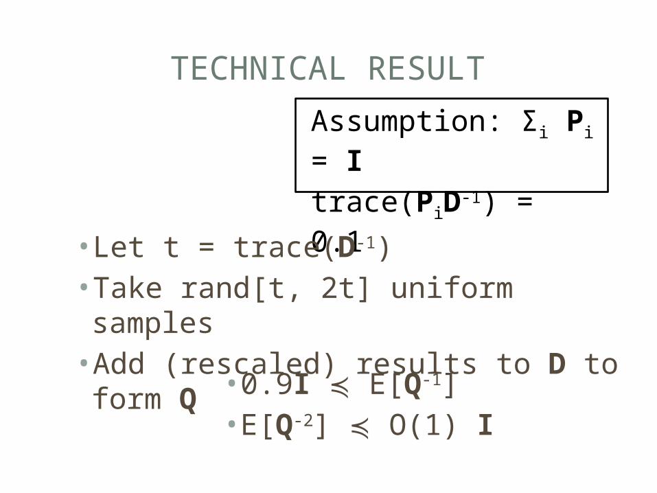
TECHNICAL RESULT

Assumption: Σi Pi = Itrace(PiD-1) = 0.1

• Let t = trace(D-1)• Take rand[t, 2t] uniform samples• Add (rescaled) results to D to form Q

• 0.9I ≼ E[Q-1]• E[Q-2] ≼ O(1) I

Q-1

• 0.5I ≼ E[Q-1] follows from matrix arithmetic-harmonic mean inequality ([ST`94])•Need: upper bound on E[Q-2]

1/2 1/2-1( )

E[Q-2] ≼ O(1) ?

•Q-2 is gradient of Q-1

•More careful tracking of Q-1 gives info on Q-2 as well!

Q-1

Q-2

j=t

j=2t

j=0

TRACKING Q-1

•Q: start from D, add [t,2t] random (rescaled) Pis.

• Track inverse of Q under rank-1 perturbations

Sherman Morrison formula:

BOUNDING Q-1: DENOMINATOR

Current matrix: Qj, sample: R

• D ≼ Qj Qj-1 ≼ D-1

• tr(Qj-1R) ≤ tr(D-1R) ≤ 0.1 for any

R,

ER[Qj+1-1] ≼ Qj

-1 – 0.9 Qj-1E[R]Qj

-

1E

BOUNDING Q-1: NUMERATOR

• R: random rescaled Pi sampled

• Assumption: E[R] = P = I

ER[Qj+1-1] ≼ Qj

-1 – 0.9/t Qj

-2

ER[Qj+1-1] ≼ Qj

-1 – 0.9 Qj-1E[R]Qj

-1

AGGREGATION

•Qj is also random

•Need to aggregate choices of R into bound on E[Qj

-1]

ER[Qj+1-1] ≼ Qj

-1 – 0.9/t Qj

-2

D = Q0

Q1

Q2

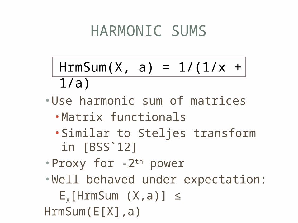
HARMONIC SUMS

• Use harmonic sum of matrices• Matrix functionals• Similar to Steljes transform in

[BSS`12]• Proxy for -2th power• Well behaved under expectation:

EX[HrmSum (X,a)] ≤ HrmSum(E[X],a)

HrmSum(X, a) = 1/(1/x + 1/a)

HARMONIC SUM

Initial condition + telescoping sum gives E[Qt

-1] ≼ O(1)I

ER[Qj+1-1] ≼ Qj

-1 – 0.9/t Qj

-2

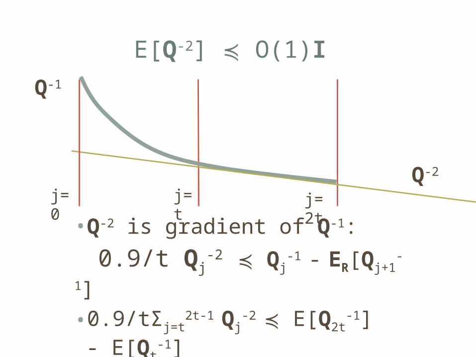
E[Q-2] ≼ O(1)I

•Q-2 is gradient of Q-1:

0.9/t Qj-2 ≼ Qj

-1 - ER[Qj+1-1]

• 0.9/tΣj=t2t-1 Qj

-2 ≼ E[Q2t-1] - E[Qt

-

1]• Random j from [t,2t] is good!

Q-1

j=t

j=2t

j=0

Q-2

SUMMARY

Un-normalize:• 0.5 P ≼ E[PQ-1P]• E[PQ-1PQ-1P] ≼ 5P

One step of preconditioned Richardson:

MORE GENERAL

•Works for some convex functions• Sherman-Morrison replaced by inequality, primal/dual

FUTURE WORK

• Expected convergence of• Chebyshev iteration?• Conjugate gradient?

• Same bound without D (using pseudo-inverse)?• Small error settings• Stochastic optimization?• More moments?

THANK YOU!

Questions?