precision cosmology with gaussian processes -...

Salman Habib, Benasque workshop, August 2010

Precision cosmology requires dealing with (i) expensive state of the art simulations, (ii) large number of dimensions, (iii) regression (input-output relationships), (iv) estimation and control of errors, (v) regularizing and solving ill-posed inverse problems (given data, estimate model parameters)

In solving regression and inverse problems (both of which may be considered as problems in Bayesian inference) one has to make choices about characteristic functions by either (i) restricting attention to a single type (linear) or class of functions (polynomials), or (ii) assign prior probabilities to classes of functions, with some considered more likely (due to smoothness, say)

Gaussian Processes (GPs) provide a surprisingly computationally effective method with which to apply the latter approach; now becoming increasingly popular (in latest edition of Numerical Recipes)

We have applied the GP in several places: (i) the COSMIC CALIBRATION framework (talk by Katrin), (ii) photo-z estimation, (iii) w(z) reconstruction from Sn data, ---

Precision Cosmology with Gaussian ProcessesU. Alam, D. Bingham, SH, K. Heitmann, D. Higdon, T. Holsclaw,

L. Knox, E. Lawrence, H. Lee, C. Nakhleh, B. Sanso, M. Schneider, M. White, B. Williams, ---

LA-UR 08-07921, 09-05888

Monday, August 9, 2010

Bayesian Approach: Basics

Prior distribution over random functions: global mean zero (although individual choices clearly are not mean-zero), variance assumed to be independent of x, 2-SD band in gray

Posterior distribution conditioned on exact information at two x points, consider only those functions from the prior distribution that pass through these points

Acceptable functions

Mean value function (not mean zero!)

Rasmussen & Williams 2006

Reduction in posterior uncertainty

GPs are nonparametric, so there is no need to worry if the functions can fit the data (e.g., linear functions against nonlinear data), even with many observations still have plenty of candidate functions

With GP models, the choice of prior distribution over random functions is essentially a statement of the properties of the initial covariance function, these properties can be specified in terms of a set of hyperparameters, using data to determine these defines the learning problem for the GP approach

Avoid overfitting by using priors on hyperparameters and by controlling the learning process (later)


GP Modeling: Basics I

GPs are straightforward generalizations of Gaussian distributions over vectors to function spaces, and are specified by a mean function and a covariance function

f = (f1, . . . , fn)T ∼ N (µ,Σ)

They have several convenient properties, of which the two most significant are

Marginalization yields a Gaussian distribution

p(ya) =�

p(ya,yb)dyb

p(ya,yb) = N��

ab

�,

�A BBT C

��=⇒ p(ya) = N (a,A)

cov(f(x), f(x�)) = k(x,x�)

f(x) ∼ GP(µ(x), k(x,x�))


GP Modeling: Basics II Conditioning yields a new Gaussian distribution

p(ya|yb) =p(ya,yb)

p(yb)

p(ya,yb) = N��

ab

�,

�A BBT C

��

=⇒ p(ya|yb) = N (a + BC−1(yb − b),A−BC−1BT )

The result also holds for conditioning with Gaussian errors. This property is important because it means that conditioning can be carried out “analytically”, without a brute force rejection algorithm being employed.

Note, however, that a matrix inversion is required for this step. This is one aspect of the “curse of dimensionality” in regression/inverse problems. Ideas on how to deal with this issue are at the cutting edge of current research.


GP Modeling: Basics IIISimple illustration of the conditioning formula in 2 dimensions for a mean-zero Gaussian process:

p(yb|ya,Σ) =p(ya, yb|Σ)

p(ya|Σ)∝ exp−1

2

�(ya yb)

�a bb c

� �ya

yb

��consts. absorbed in normalization, since is known ya

= exp−12

�ay2

a + 2byayb + cy2b

�∝ exp−1

2�2byayb + cy2

b

�

∝ exp−12

��y2

b + 2b

cyayb +

b2

c2y2

a

�c

�

= exp−12

��yb −

�− b

cya

��2

c−1

�

y₁

y₂Diagonal

Covariancewith a=c

Non-trivial Covariance

Even though the joint distributionof y1 and y2 is mean-zero, the conditioned distribution of y2 is not mean-zero, if the covariance matrix is not diagonal


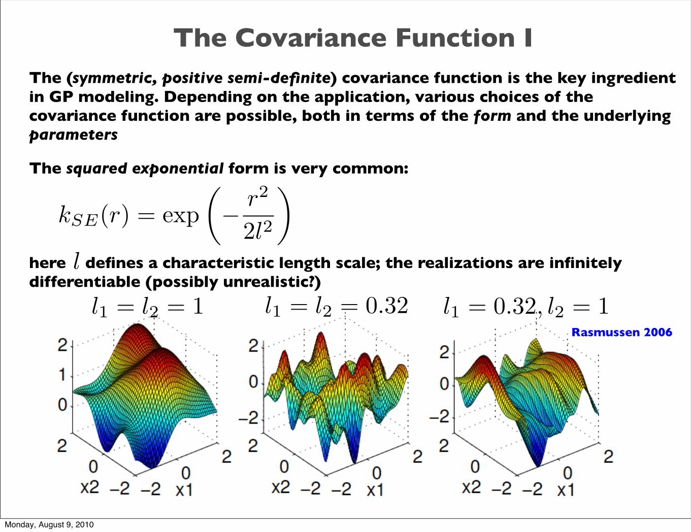
The Covariance Function IThe (symmetric, positive semi-definite) covariance function is the key ingredient in GP modeling. Depending on the application, various choices of the covariance function are possible, both in terms of the form and the underlying parameters

The squared exponential form is very common:

here defines a characteristic length scale; the realizations are infinitely differentiable (possibly unrealistic?)

kSE(r) = exp�− r2

2l2

�

l

l1 = l2 = 1 l1 = l2 = 0.32 l1 = 0.32, l2 = 1Rasmussen 2006


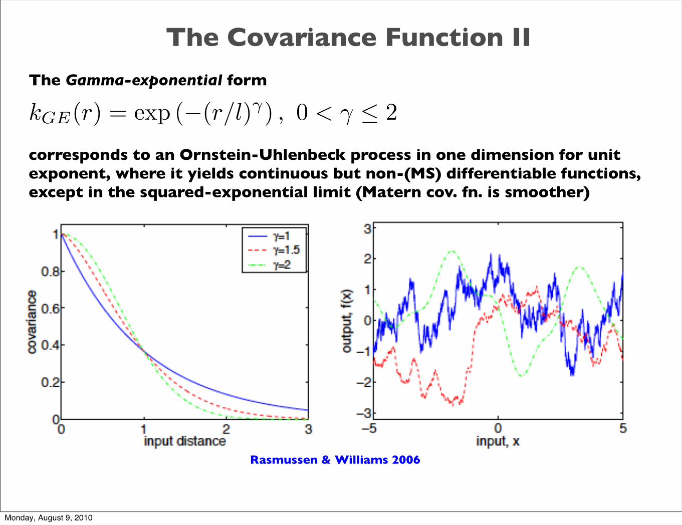
The Covariance Function II

The Gamma-exponential form

corresponds to an Ornstein-Uhlenbeck process in one dimension for unit exponent, where it yields continuous but non-(MS) differentiable functions, except in the squared-exponential limit (Matern cov. fn. is smoother)

kGE(r) = exp (−(r/l)γ) , 0 < γ ≤ 2

Rasmussen & Williams 2006


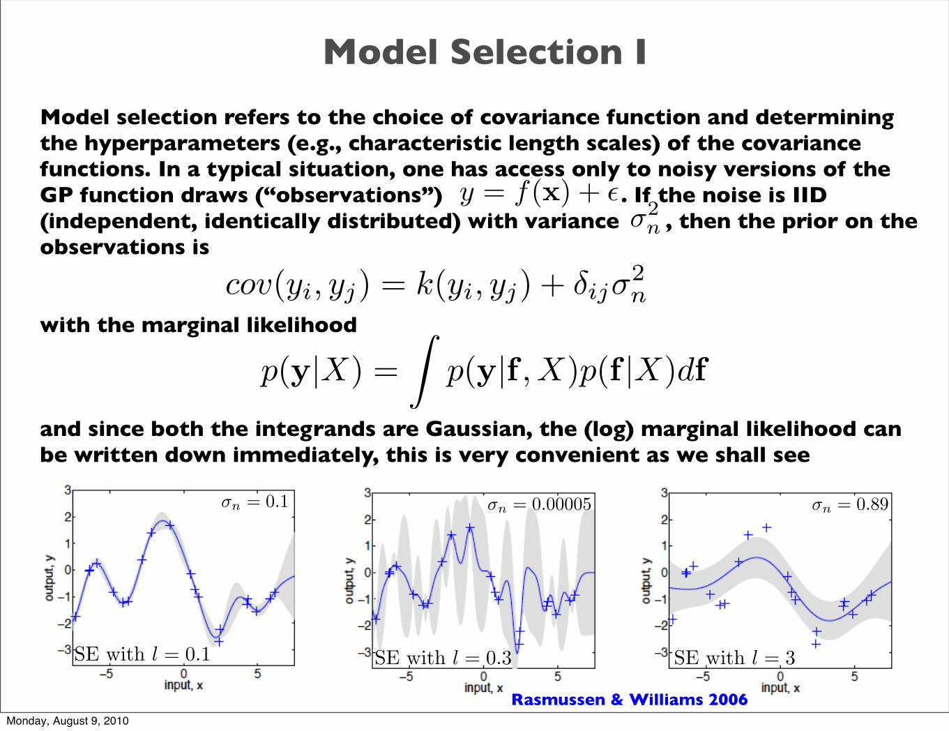
Model Selection I

Model selection refers to the choice of covariance function and determining the hyperparameters (e.g., characteristic length scales) of the covariance functions. In a typical situation, one has access only to noisy versions of the GP function draws (“observations”) . If the noise is IID (independent, identically distributed) with variance , then the prior on the observations is

with the marginal likelihood

and since both the integrands are Gaussian, the (log) marginal likelihood can be written down immediately, this is very convenient as we shall see

y = f(x) + �σ2

n

cov(yi, yj) = k(yi, yj) + δijσ2n

p(y|X) =�

p(y|f , X)p(f |X)df

SE with l = 0.1 SE with l = 0.3 SE with l = 3

σn = 0.1 σn = 0.00005 σn = 0.89

Rasmussen & Williams 2006Monday, August 9, 2010

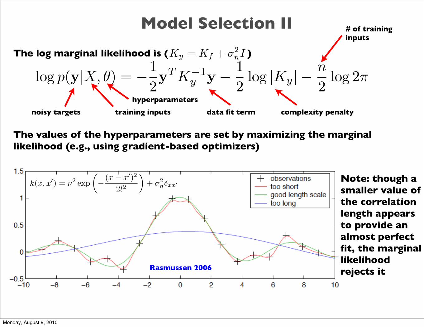
Model Selection II

The log marginal likelihood is ( )

The values of the hyperparameters are set by maximizing the marginal likelihood (e.g., using gradient-based optimizers)

log p(y|X, θ) = −12yT K−1

y y − 12

log |Ky|− n

2log 2π

hyperparameters

training inputsnoisy targets

# of training inputs

Ky = Kf + σ2nI

data fit term complexity penalty

k(x, x�) = ν2 exp�− (x− x�)2

2l2

�+ σ2

nδxx�

Rasmussen 2006

Note: though a smaller value of the correlation length appears to provide an almost perfect fit, the marginal likelihood rejects it


Wrap-Up/Issues

Many additional issues show up in actual practice:

GPs can be applied directly to data or to weights of basis functions used to represent the data (e.g., to a Principal Components basis, more later)

Robustness of results -- would prefer if answers were not too touchy as a function of choice of covariance function (usually the case)

How good is the naive GP error theory in actual practice? How can one validate the procedure (more on hold-out tests and sub-sampling)? Important in cosmology applications with stringent error control requirements

Use of weighted sampling and iterative procedures allowed within the GP approach, can be extended to covariances (Schneider et al 2008)

Using fast surrogate models is a good way to build confidence in the GP approach and to optimize it

Approximate methods to reduce the scaling due to the matrix inverse computation (e.g., compact support covariance functions)

Prediction outside the fitted range of a GP is a bad idea

N3


Application I: w(z) Reconstruction How to approach the dark energy characterization problem?

(i) Show convincingly it’s not a cosmological constant

(ii) Given (i), try parameterized models or physically well-motivated ideas (ha!), worries about possible biases due to incompatibility with the data

(iii) Hypothesis testing to attempt to rule out classes of DE models (sort of the next step after (i))

(iv) Reconstruct w(z) directly from data, very hard because of the double integral smoothing operator that must be inverted (smoothing data and then differentiating is a bad idea)

Simple case: Distance modulus for a spatially flat FRW cosmology

Example reconstruction problem for ‘JDEM’ + 300 low-z supernovae

Holsclaw et al 2010


GP for w(z) I

Assume a GP for the DE EOS parameter

Need to integrate over this in the expression for the distance modulus, where

The integral of a GP is another GP, and assuming a gamma-exponential form of the covariance

A joint GP for the two variables can be constructed:

w(u) ∼ GP(−1, K(u, u�))

y(s) =� s

o

w(u)1 + u

du

y(s) ∼ GP�− ln(1 + s), κ2

� s

0

� s�

0

ρ|u−u�|αdudu�

(1 + u)(1 + u�)

�

�y(s)w(u)

�∼ GP

��− ln(1 + s)

−1

�,

�Σ11 Σ12

Σ21 Σ22

��


GP for w(z) IIwhere

The mean for given is

so the expensive double integral does not have to be computed. Now that the GP model has been constructed one follows the procedure outlined earlier, ‘fits’ to the data, and extracts (the details of the procedure are actually rather complicated and are given in a forthcoming paper, Holsclaw et al. 2010)

Depending on the assumptions made about the data, we find that smooth infinitely differentiable functions fit the current observations well, but that for simulated data we have to take a much smaller value for the power exponent in the covariance function

y(s) w(u)

Σ11

w(z)


GP Reconstruction on ‘Future’ Data

Using ‘JDEM’ simulateddata mocking up smooth, but devious DE EOS histories, we can check if the GP model can correctly reconstruct them

Results are encouragingas can be seen here with an ‘extreme’ quintessence model

Smoother DE EOS histories are recovered well

GP model readjusts mean starting from -1 to -0.7

95%

68%

Predicted mean

Exponential covariance function Holsclaw et al 2010


GP Reconstruction on Current Data

Using results from the ‘Constitution’ dataset Hicken et al (2009) and WMAP7 priors, the GP-based reconstruction finds no evidence of a deviation from the cosmological constant

The GP methodology allows the integration of multiple datasets and sources of information within an overall Bayesian framework, work on adding CMB and BAO data is almost complete

The GP, as used here, has many useful features: (i) the data is not massaged in any way, (ii) robustness of results to variations of GP hyperparameters can be easily tested, (iii) degeneracies are automatically found during the fitting process

68%

95%

95%

68%

Predicted mean

Squared exponential covariance function

Exponential covariance function

Holsclaw et al 2010


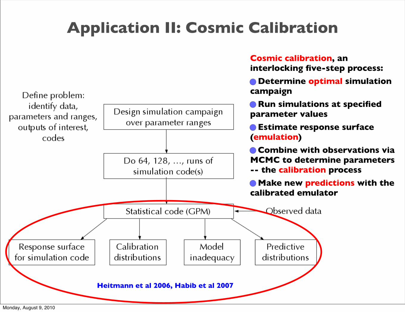
Application II: Cosmic Calibration

Cosmic calibration, an interlocking five-step process:

Determine optimal simulation campaign

Run simulations at specified parameter values

Estimate response surface (emulation)

Combine with observations via MCMC to determine parameters -- the calibration process

Make new predictions with the calibrated emulator

Heitmann et al 2006, Habib et al 2007


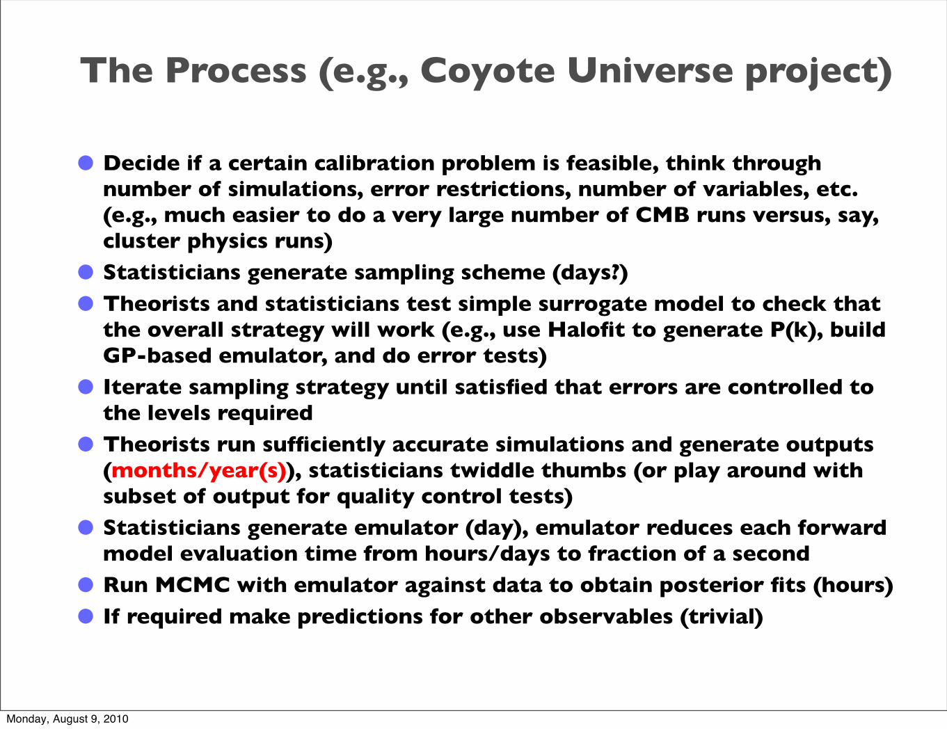
• Decide if a certain calibration problem is feasible, think through number of simulations, error restrictions, number of variables, etc. (e.g., much easier to do a very large number of CMB runs versus, say, cluster physics runs)

• Statisticians generate sampling scheme (days?)

• Theorists and statisticians test simple surrogate model to check that the overall strategy will work (e.g., use Halofit to generate P(k), build GP-based emulator, and do error tests)

• Iterate sampling strategy until satisfied that errors are controlled to the levels required

• Theorists run sufficiently accurate simulations and generate outputs (months/year(s)), statisticians twiddle thumbs (or play around with subset of output for quality control tests)

• Statisticians generate emulator (day), emulator reduces each forward model evaluation time from hours/days to fraction of a second

• Run MCMC with emulator against data to obtain posterior fits (hours)

• If required make predictions for other observables (trivial)

The Process (e.g., Coyote Universe project)


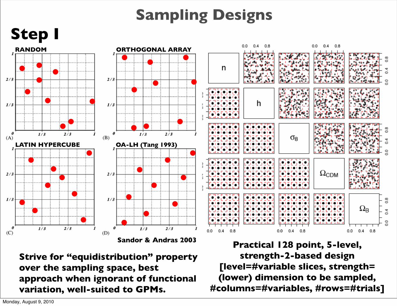
Sampling Designs

Practical 128 point, 5-level, strength-2-based design

[level=#variable slices, strength=(lower) dimension to be sampled,

#columns=#variables, #rows=#trials]

Sandor & Andras 2003

RANDOM ORTHOGONAL ARRAY

LATIN HYPERCUBE OA-LH (Tang 1993)

Strive for “equidistribution” propertyover the sampling space, best approach when ignorant of functional variation, well-suited to GPMs.

Step I


Basis Representation of Simulated SpectraP(k) example

SIMULATIONS MEAN FIRST 5 PCs

Mean-adjusted Principal Component Representation

COSMOLOGICAL/MODELING PARAMETERS

PC BASIS FUNCTIONS

GP WEIGHTSSTANDARDIZED

PARAMETER DOMAIN

Step II

Heitmann et al 2006


Gaussian Process ModelingStep III

HOLDOUT TEST


Test of the Emulator -II


128 RUN DESIGN 32 RUN DESIGN

ERRORS vs. 64 RUN REFERENCE DESIGN

90%

50%

90%

50%

k

90%90%

50%50%

128 RUNS, ORDER OF MAGNITUDE IMPROVEMENTWITH CONSTRAINED PRIORS (WMAP-3SIGMA)

worst-case outliers

P(k)

C_l

+/-5% +/-0.5%

More on Convergence: Post Hold-Out

Habib et al 2007


Results: CMB + P(k)(simulated data plus 128/128 runs, 6 parameters)

Estimate parameters: explore posterior distribution via MCMC taking emulation errors into account.

Framework simultaneously handles C_l and P(k) emulation; other inputs can be easily added. Here P(k) simulated data was “SDSS main sample”.

Very good results from a small number of base simulations.

Target points correspond to the values at which the simulated data were generated.

Step IV


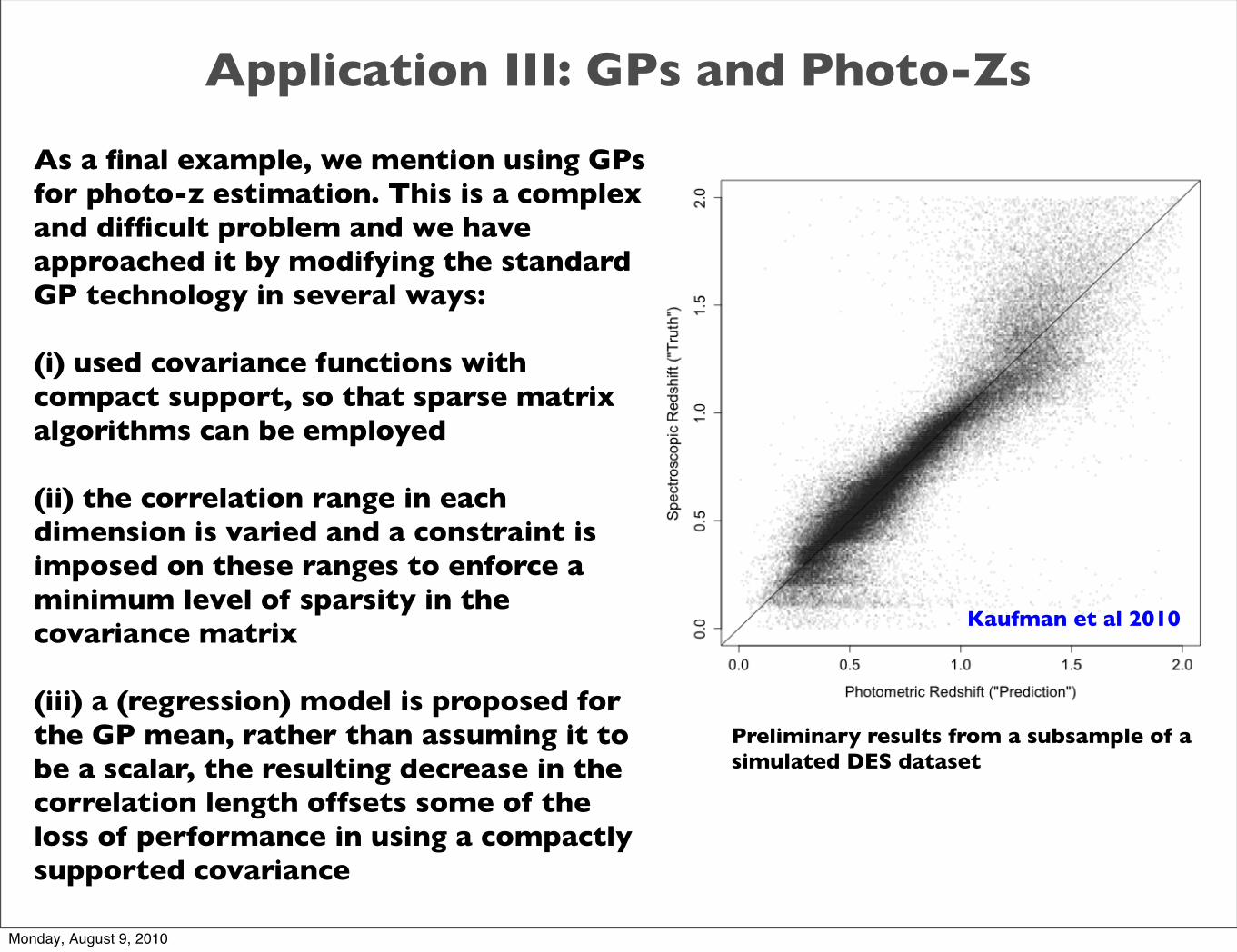
Application III: GPs and Photo-Zs

As a final example, we mention using GPs for photo-z estimation. This is a complex and difficult problem and we have approached it by modifying the standard GP technology in several ways:

(i) used covariance functions with compact support, so that sparse matrix algorithms can be employed

(ii) the correlation range in each dimension is varied and a constraint is imposed on these ranges to enforce a minimum level of sparsity in the covariance matrix

(iii) a (regression) model is proposed for the GP mean, rather than assuming it to be a scalar, the resulting decrease in the correlation length offsets some of the loss of performance in using a compactly supported covariance

Preliminary results from a subsample of a simulated DES dataset

Kaufman et al 2010


• www.GaussianProcess.org

• C.E. Rasmussen & C.K.I. Williams, Gaussian Processes for Machine Learning, MIT Press, 2006, available at www.GaussianProcess.org/gpml

• D.J.C. MacKay, Information Theory, Inference, and Learning Algorithms, Cambridge University Press, 2003

• D. Higdon et al in the Oxford Handbook of Applied Bayesian Analysis, edited by A. O’Hagan & M. West, Oxford University Press, 2010

• M. Kennedy & A. O’Hagan, Bayesian Calibration of Computer Models (with discussion), J. Roy. Stat. Soc. 68, 425 (2001)

GP Resources

Proof that progress occurs in interpolation methods (Bleau, Thevenaz, & Unser 2004)


http://www.GaussianProcess.org/gpml

http://www.GaussianProcess.org/gpml

precision cosmology with gaussian processes -...

Documents