Precipitation

• Type of Precipitation

• Measurement of rainfall

• Location of rain gauges

• Categorisation Climate

• Estimation of basin rainfall

• Finding Average rainfall, Standard deviation, and Coefficient of variation(%) in a basin

• Rainfall analysis

– Recurrence interval or return period

– Depth Area and duration curves

– Mass curve and Hyetograph

– Maximum Depth-Duration & intensity curves

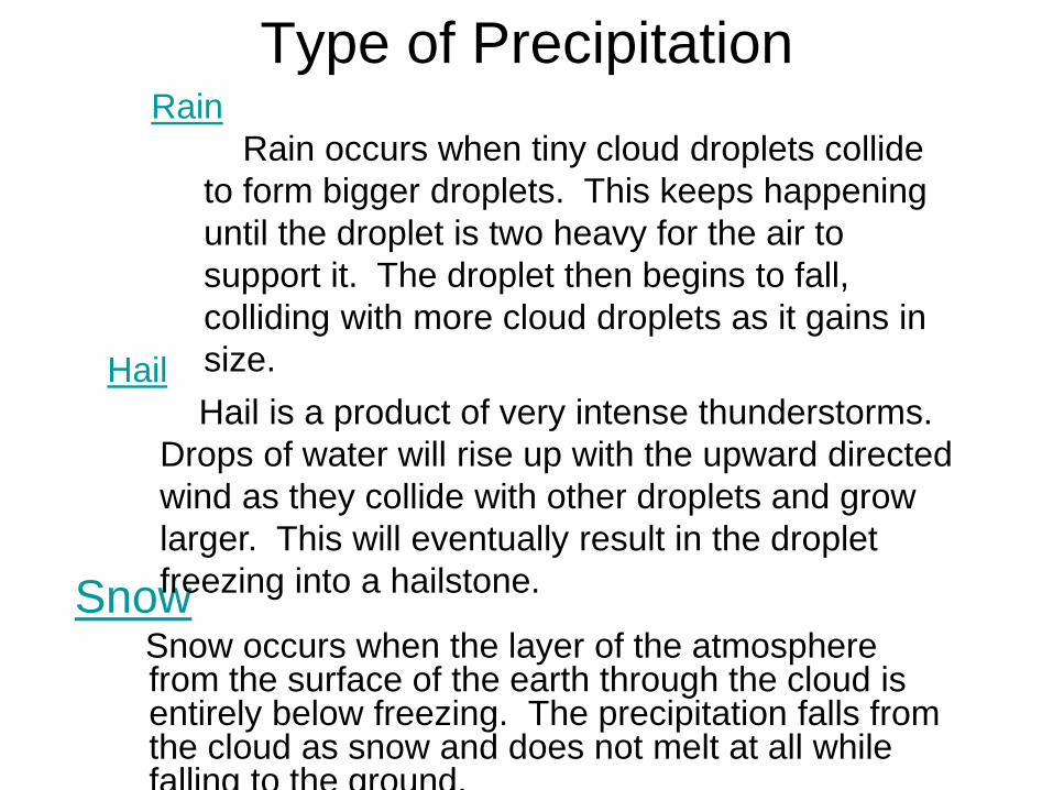
Type of Precipitation

Snow Snow occurs when the layer of the atmosphere

from the surface of the earth through the cloud is entirely below freezing. The precipitation falls from the cloud as snow and does not melt at all while falling to the ground.

Rain

Rain occurs when tiny cloud droplets collide

to form bigger droplets. This keeps happening

until the droplet is two heavy for the air to

support it. The droplet then begins to fall,

colliding with more cloud droplets as it gains in

size. Hail

Hail is a product of very intense thunderstorms.

Drops of water will rise up with the upward directed

wind as they collide with other droplets and grow

larger. This will eventually result in the droplet

freezing into a hailstone.

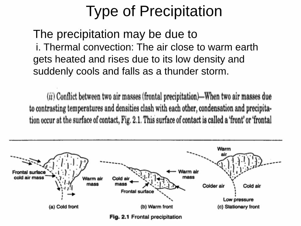
Type of Precipitation

The precipitation may be due to

i. Thermal convection: The air close to warm earth

gets heated and rises due to its low density and

suddenly cools and falls as a thunder storm.

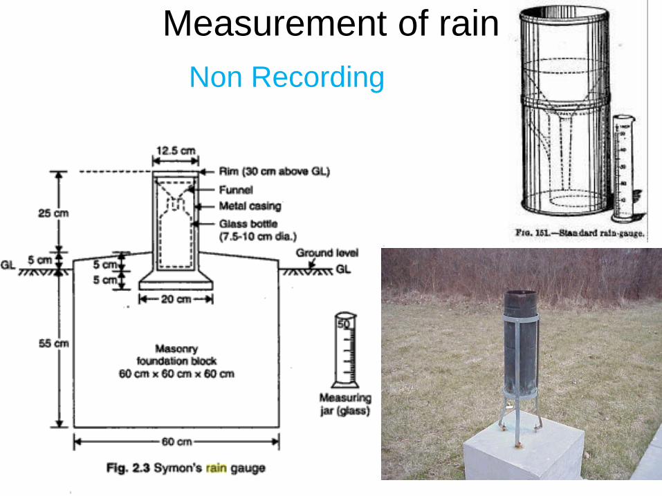
Measurement of rain

Non Recording

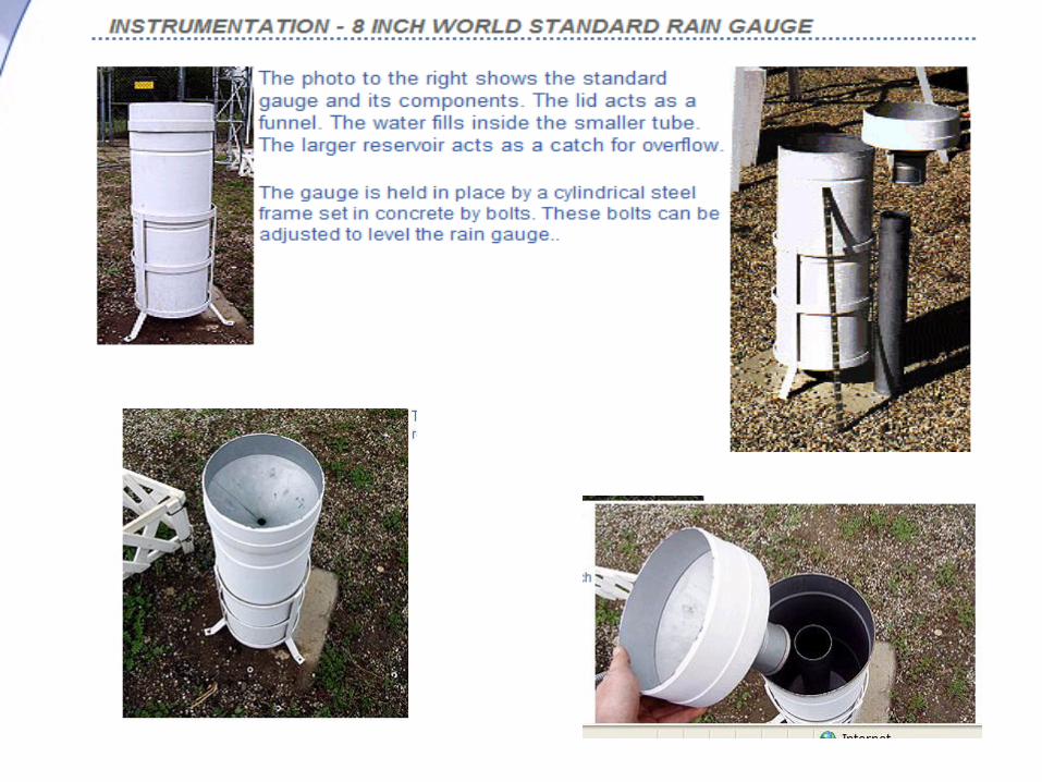
Recording/ Automatic rain gauges

Radio reporting rain gauges

Radars

Location of rain gauges

• Rain gauges must be located to avoid

exposure to wind effect or interception by

trees or buildings. The best location is an

oen plan ground like air ports

Density of rain gauges Plains one in 520 km^2

Elevated regions one in 520 km^2

Hilly and very heavy rainfall areas one in 130 km^2 and 10%

should be automatic raingauges

In India on an average 1 on 500 km^2

In developed countries 1 in 100 km^2

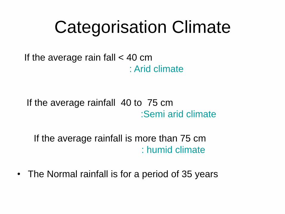
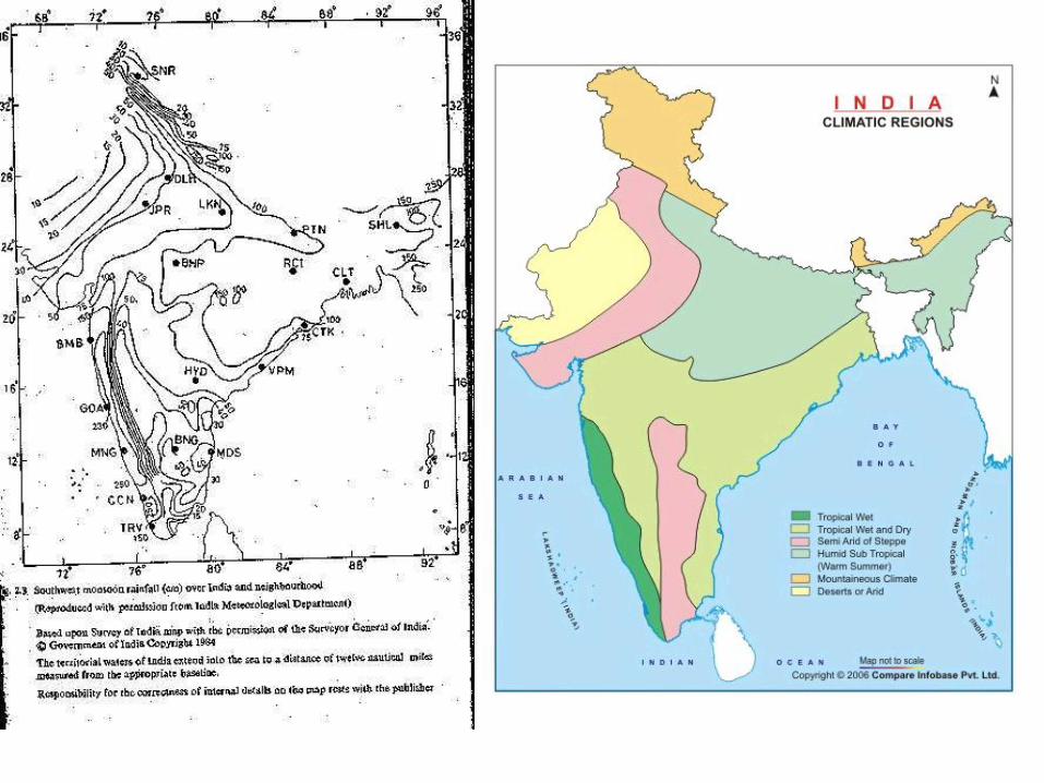
Categorisation Climate

• The Normal rainfall is for a period of 35 years

If the average rain fall < 40 cm

: Arid climate

If the average rainfall 40 to 75 cm

:Semi arid climate

If the average rainfall is more than 75 cm

: humid climate

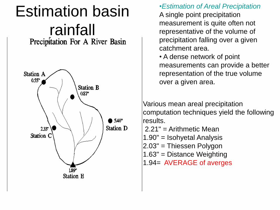
•Estimation of Areal Precipitation

A single point precipitation

measurement is quite often not

representative of the volume of

precipitation falling over a given

catchment area.

• A dense network of point

measurements can provide a better

representation of the true volume

over a given area.

Estimation basin

rainfall

Various mean areal precipitation

computation techniques yield the following

results.

2.21" = Arithmetic Mean

1.90" = Isohyetal Analysis

2.03" = Thiessen Polygon

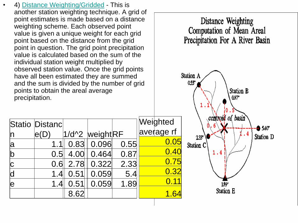
1.63" = Distance Weighting

1.94= AVERAGE of averges

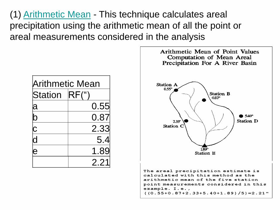
(1) Arithmetic Mean - This technique calculates areal

precipitation using the arithmetic mean of all the point or

areal measurements considered in the analysis

Arithmetic Mean

Station RF(“)

a 0.55

b 0.87

c 2.33

d 5.4

e 1.89

2.21

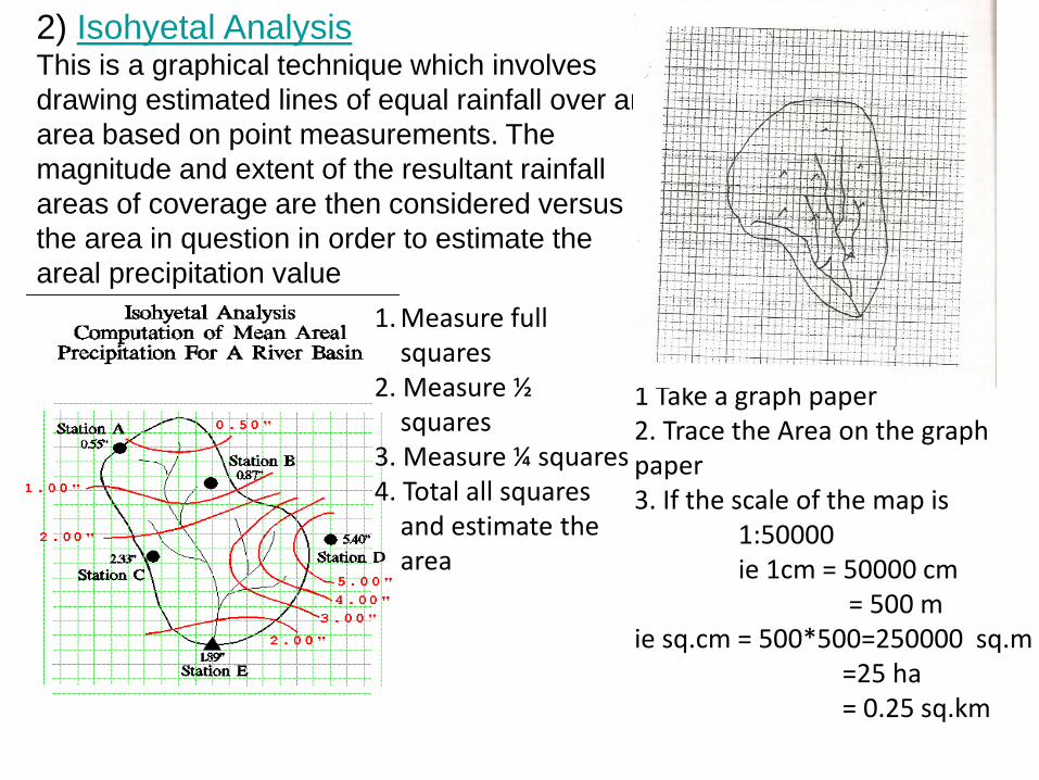
2) Isohyetal Analysis This is a graphical technique which involves

drawing estimated lines of equal rainfall over an

area based on point measurements. The

magnitude and extent of the resultant rainfall

areas of coverage are then considered versus

the area in question in order to estimate the

areal precipitation value

1 Take a graph paper 2. Trace the Area on the graph paper 3. If the scale of the map is 1:50000 ie 1cm = 50000 cm = 500 m ie sq.cm = 500*500=250000 sq.m =25 ha = 0.25 sq.km

1. Measure full squares

2. Measure ½ squares

3. Measure ¼ squares 4. Total all squares

and estimate the area

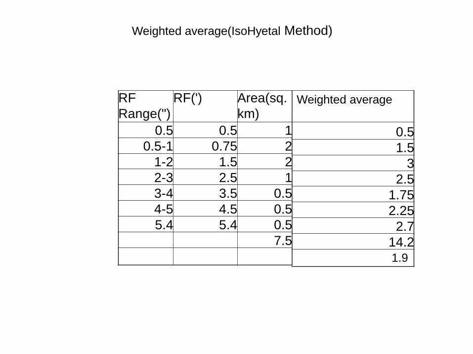
RF

Range(")

RF(') Area(sq.

km)

0.5 0.5 1

0.5-1 0.75 2

1-2 1.5 2

2-3 2.5 1

3-4 3.5 0.5

4-5 4.5 0.5

5.4 5.4 0.5

7.5

0.5

1.5

3

2.5

1.75

2.25

2.7

14.2

Weighted average(IsoHyetal Method)

Weighted average

1.9

Weighted

8.25

28.71

67.104

88.56

45.927

238.551

2.03

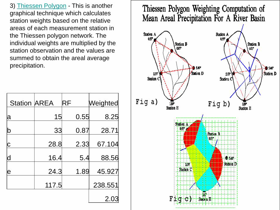
3) Thiessen Polygon - This is another

graphical technique which calculates

station weights based on the relative

areas of each measurement station in

the Thiessen polygon network. The

individual weights are multiplied by the

station observation and the values are

summed to obtain the areal average

precipitation.

Station AREA RF

a 15 0.55

b 33 0.87

c 28.8 2.33

d 16.4 5.4

e 24.3 1.89

117.5

Weighted

average rf

0.05

0.40

0.75

0.32

0.11

1.64

• 4) Distance Weighting/Gridded - This is another station weighting technique. A grid of point estimates is made based on a distance weighting scheme. Each observed point value is given a unique weight for each grid point based on the distance from the grid point in question. The grid point precipitation value is calculated based on the sum of the individual station weight multiplied by observed station value. Once the grid points have all been estimated they are summed and the sum is divided by the number of grid points to obtain the areal average precipitation. Statio

n

Distanc

e(D) 1/d^2 weight RF

a 1.1 0.55

b 0.5 0.87

c 0.6 2.33

d 1.4 5.4

e 1.4 1.89

0.83

4.00

2.78

0.51

0.51

8.62

0.096

0.464

0.322

0.059

0.059

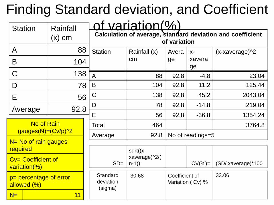
Finding Standard deviation, and Coefficient

of variation(%)

B 104 92.8 11.2 125.44

C 138 92.8 45.2 2043.04

D 78 92.8 -14.8 219.04

E 56 92.8 -36.8 1354.24

Total 464 3764.8

Average 92.8 No of readings=5

No of Rain

gauges(N)=(Cv/p)^2

N= No of rain gauges

required

Cv= Coefficient of

variation(%)

p= percentage of error

allowed (%)

N= 11

Station Rainfall

(x) cm

A 88

B 104

C 138

D 78

E 56

Average 92.8

Calculation of average, standard deviation and coefficient

of variation

Station Rainfall (x)

cm

Avera

ge

x-

xavera

ge

(x-xaverage)^2

Standard

deviation

(sigma)

30.68

Coefficient of

Variation ( Cv) %

33.06

A 88 92.8 -4.8 23.04

SD=

sqrt((x-

xaverage)^2/(

n-1)) CV(%)= (SD/ xaverage)*100

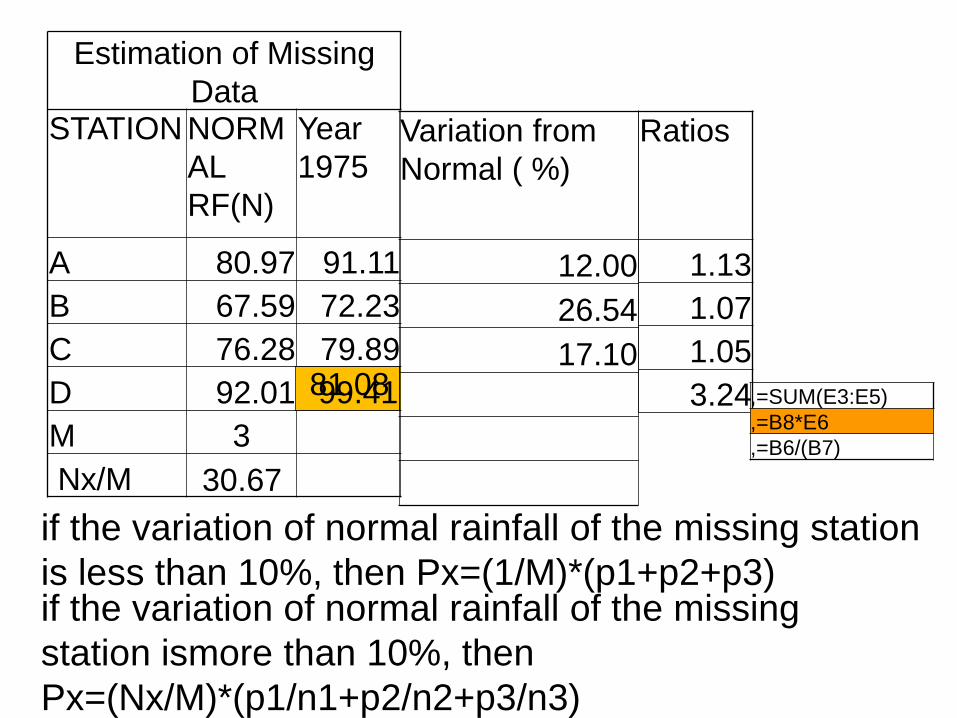
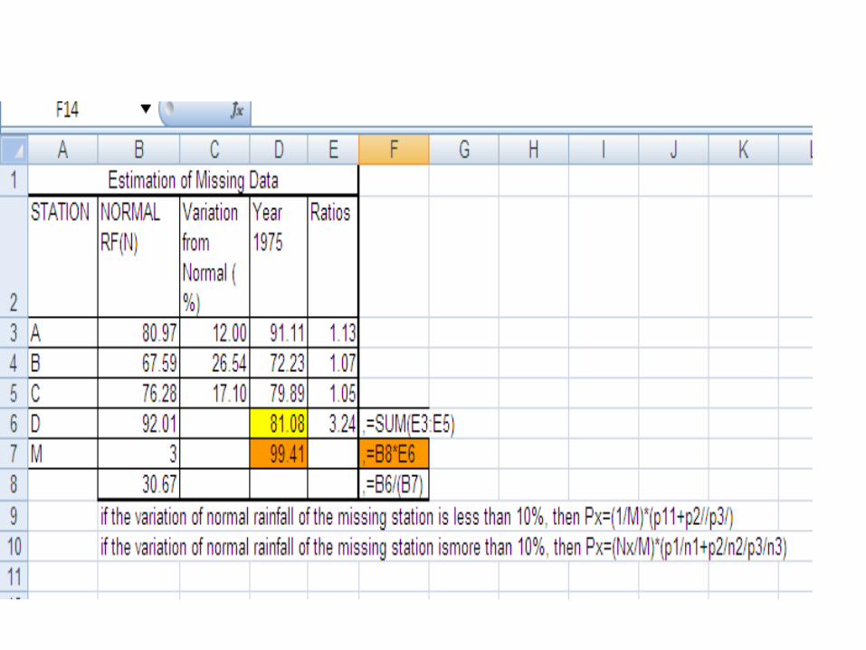
Estimation of Missing

Data STATION NORM

AL

RF(N)

Year

1975

A 80.97 91.11

B 67.59 72.23

C 76.28 79.89

D 92.01

M 3

Nx/M

if the variation of normal rainfall of the missing station

is less than 10%, then Px=(1/M)*(p1+p2+p3) if the variation of normal rainfall of the missing

station ismore than 10%, then

Px=(Nx/M)*(p1/n1+p2/n2+p3/n3)

Variation from

Normal ( %)

12.00

26.54

17.10

99.41 81.08

Ratios

1.13

1.07

1.05

3.24

30.67

,=SUM(E3:E5)

,=B8*E6

,=B6/(B7)

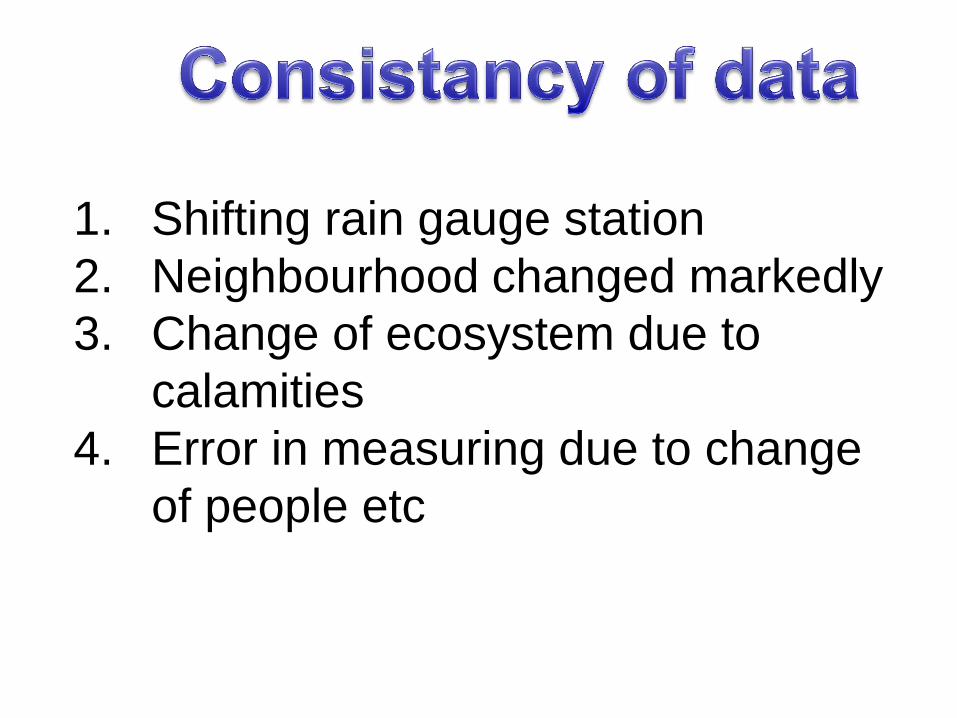
1. Shifting rain gauge station

2. Neighbourhood changed markedly

3. Change of ecosystem due to

calamities

4. Error in measuring due to change

of people etc

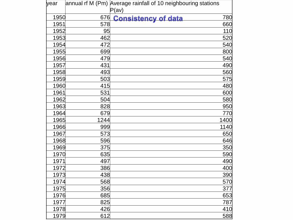
year annual rf M (Pm) Average rainfall of 10 neighbouring stations

P(av)

1950 676 780

1951 578 660

1952 95 110

1953 462 520

1954 472 540

1955 699 800

1956 479 540

1957 431 490

1958 493 560

1959 503 575

1960 415 480

1961 531 600

1962 504 580

1963 828 950

1964 679 770

1965 1244 1400

1966 999 1140

1967 573 650

1968 596 646

1969 375 350

1970 635 590

1971 497 490

1972 386 400

1973 438 390

1974 568 570

1975 356 377

1976 685 653

1977 825 787

1978 426 410

1979 612 588

year annual rf M(Pm)

(mm)

Cummulaative RF Average rainfall of 10

neighbouring stations (Pav) (mm)

Cummulaative

RF (avg)

1979 612 612 588 588

1978 426 1038 410 998

1977 825 1863 787 1785

1976 685 2548 653 2438

1975 356 2904 377 2815

1974 568 3472 570 3385

1973 438 3910 390 3775

1972 386 4296 400 4175

1971 497 4793 490 4665

1970 635 5428 590 5255

1969 375 5803 350 5605

1968 596 6399 646 6251

1967 573 6972 650 6901

1966 999 7971 1140 8041

1965 1244 9215 1400 9441

1964 679 9894 770 10211

1963 828 10722 950 11161

1962 504 11226 580 11741

1961 531 11757 600 12341

1960 415 12172 480 12821

1959 503 12675 575 13396

1958 493 13168 560 13956

1957 431 13599 490 14446

1956 479 14078 540 14986

1955 699 14777 800 15786

1954 472 15249 540 16326

1953 462 15711 520 16846

1952 95 15806 110 16956

1951 578 16384 660 17616

1950 676 17060 780 18396

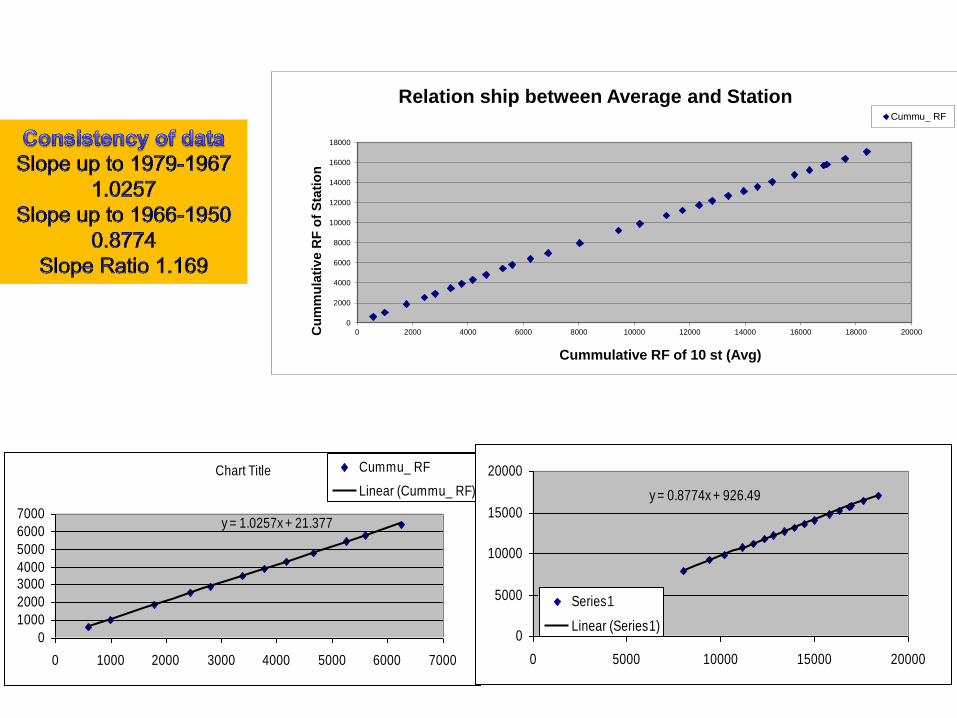
Chart Title

y = 1.0257x + 21.377

0

1000

2000

30004000

5000

6000

7000

0 1000 2000 3000 4000 5000 6000 7000

Cummu_ RF

Linear (Cummu_ RF) y = 0.8774x + 926.49

0

5000

10000

15000

20000

0 5000 10000 15000 20000

Series1

Linear (Series1)

0

2000

4000

6000

8000

10000

12000

14000

16000

18000

0 2000 4000 6000 8000 10000 12000 14000 16000 18000 20000Cu

mm

ula

tiv

e R

F o

f S

tati

on

Cummulative RF of 10 st (Avg)

Relation ship between Average and Station Cummu_ RF

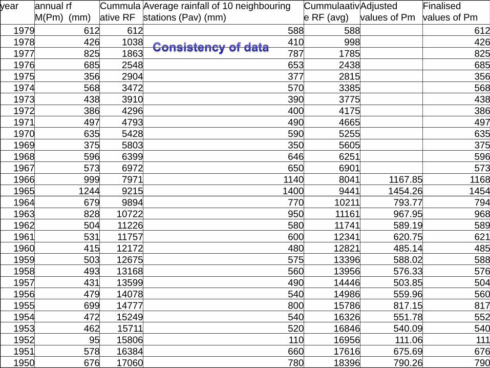
year annual rf

M(Pm) (mm)

Cummula

ative RF

Average rainfall of 10 neighbouring

stations (Pav) (mm)

Cummulaativ

e RF (avg)

Adjusted

values of Pm

Finalised

values of Pm

1979 612 612 588 588 612

1978 426 1038 410 998 426

1977 825 1863 787 1785 825

1976 685 2548 653 2438 685

1975 356 2904 377 2815 356

1974 568 3472 570 3385 568

1973 438 3910 390 3775 438

1972 386 4296 400 4175 386

1971 497 4793 490 4665 497

1970 635 5428 590 5255 635

1969 375 5803 350 5605 375

1968 596 6399 646 6251 596

1967 573 6972 650 6901 573

1966 999 7971 1140 8041 1167.85 1168

1965 1244 9215 1400 9441 1454.26 1454

1964 679 9894 770 10211 793.77 794

1963 828 10722 950 11161 967.95 968

1962 504 11226 580 11741 589.19 589

1961 531 11757 600 12341 620.75 621

1960 415 12172 480 12821 485.14 485

1959 503 12675 575 13396 588.02 588

1958 493 13168 560 13956 576.33 576

1957 431 13599 490 14446 503.85 504

1956 479 14078 540 14986 559.96 560

1955 699 14777 800 15786 817.15 817

1954 472 15249 540 16326 551.78 552

1953 462 15711 520 16846 540.09 540

1952 95 15806 110 16956 111.06 111

1951 578 16384 660 17616 675.69 676

1950 676 17060 780 18396 790.26 790

Rainfall analysis and graphical

presentation Sr.No Year Rainfall

(c

m)

1 1950 50

2 1951 60

3 1952 40

4 1953 27

5 1954 30

6 1955 38

7 1956 70

8 1957 60

9 1958 35

10 1959 55

11 1960 40

12 1961 56

13 1962 52

14 1963 42

15 1964 38

16 1965 27

17 1966 40

18 1967 100

19 1968 90

20 1969 43

21 1970 33

Let us calculate

•Mean •Median

•Moving Average

•Return period /Frequency

/Probability of certain

rainfall

Year Rainfall (cm)

1967 100

1968 90

1956 70

1951 60

1957 60

1961 56

1959 55

1962 52

1950 50

1969 43

1963 42

1952 40

1960 40

1966 40

1955 38

1964 38

1958 35

1970 33

1954 30

1953 27

1965 27

•Mean- 48.9

•Median-42

0

20

40

60

80

100

120

1950

1951

1952

1953

1954

1955

1956

1957

1958

1959

1960

1961

1962

1963

1964

1965

1966

1967

1968

1969

1970

Rain

fall

(cm

)

Year

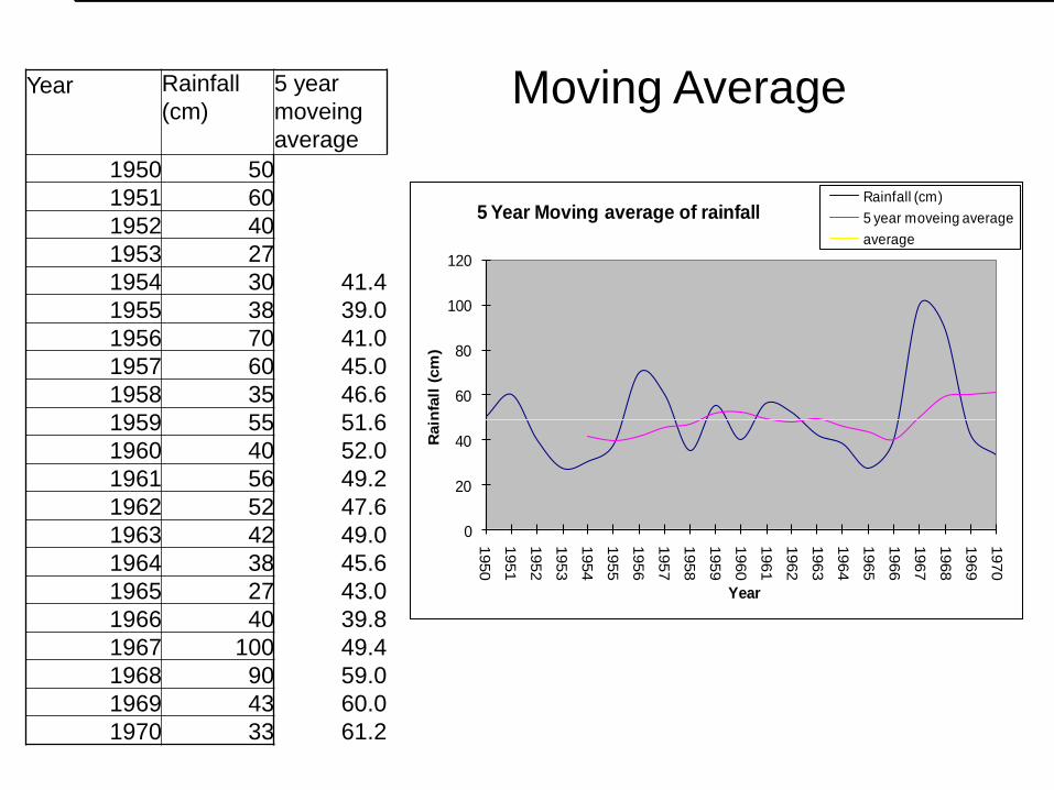
5 Year Moving average of rainfallRainfall (cm)

5 year moveing average

average

Year Rainfall

(cm)

5 year

moveing

average

1950 50

1951 60

1952 40

1953 27

1954 30 41.4

1955 38 39.0

1956 70 41.0

1957 60 45.0

1958 35 46.6

1959 55 51.6

1960 40 52.0

1961 56 49.2

1962 52 47.6

1963 42 49.0

1964 38 45.6

1965 27 43.0

1966 40 39.8

1967 100 49.4

1968 90 59.0

1969 43 60.0

1970 33 61.2

Moving Average

Year 1969 1970 1971 1972 1973 197

4

1975 197

6

1977 1978

Rainfall 215.9

0

722.

38

671.

58

119.

89

512.

06

510.

03

202.1

8

511.

05

533.40 215.39

Year 1979 1980 1981 1982 1983 198

4

1985 198

6

1987 1988

Rainfall 795.7

8

534.

42

911.

86

565.

91

1061

.97

604.

52

194.3

1

214.

88

139.95 240.03

Year 1989 1990 1991 1992 1993 199

4

1995 199

6

1997 1998

Rainfall 679.2

0

533.

40

264.

16

560.

07

325.

12

675.

64

351.0

3

303.

02

668.78 545.85

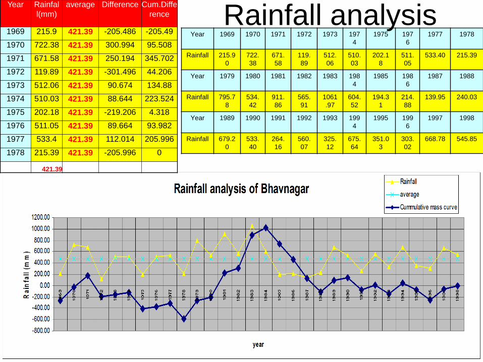
Rainfall analysis Year Rainfal

l(mm)

average Difference Cum.Diffe

rence

1969 215.9 421.39 -205.486 -205.49

1970 722.38 421.39 300.994 95.508

1971 671.58 421.39 250.194 345.702

1972 119.89 421.39 -301.496 44.206

1973 512.06 421.39 90.674 134.88

1974 510.03 421.39 88.644 223.524

1975 202.18 421.39 -219.206 4.318

1976 511.05 421.39 89.664 93.982

1977 533.4 421.39 112.014 205.996

1978 215.39 421.39 -205.996 0

421.39

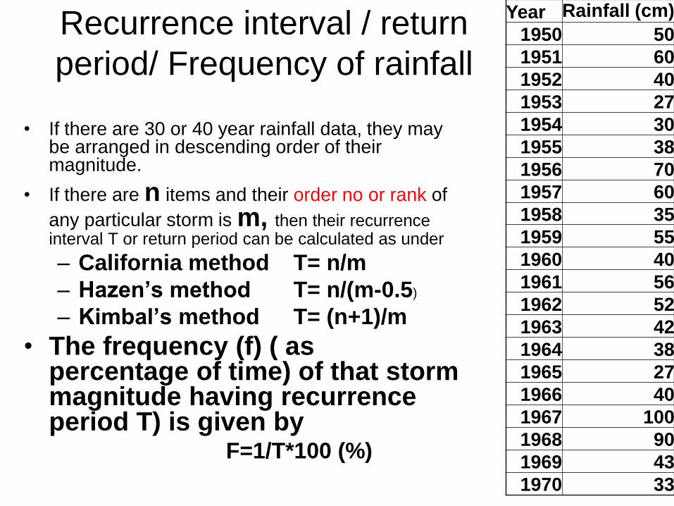
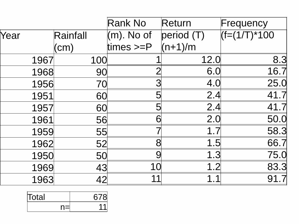
Recurrence interval / return

period/ Frequency of rainfall

• If there are 30 or 40 year rainfall data, they may be arranged in descending order of their magnitude.

• If there are n items and their order no or rank of

any particular storm is m, then their recurrence interval T or return period can be calculated as under

– California method T= n/m

– Hazen’s method T= n/(m-0.5)

– Kimbal’s method T= (n+1)/m

• The frequency (f) ( as percentage of time) of that storm magnitude having recurrence period T) is given by F=1/T*100 (%)

Year Rainfall (cm)

1950 50

1951 60

1952 40

1953 27

1954 30

1955 38

1956 70

1957 60

1958 35

1959 55

1960 40

1961 56

1962 52

1963 42

1964 38

1965 27

1966 40

1967 100

1968 90

1969 43

1970 33

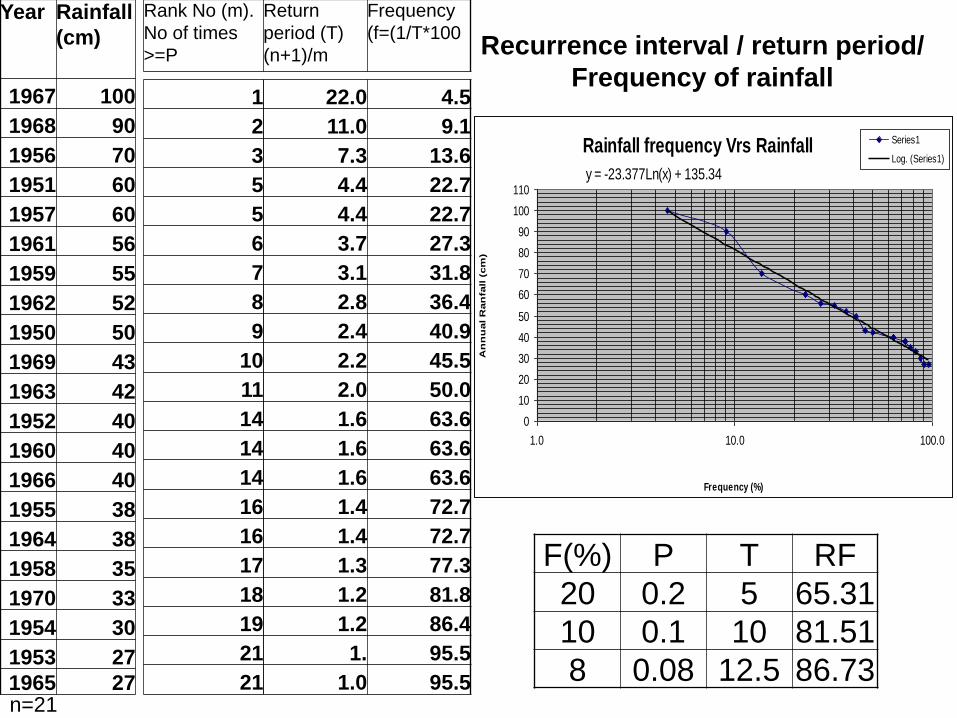
22.0 4.5

11.0 9.1

7.3 13.6

4.4 22.7

4.4 22.7

3.7 27.3

3.1 31.8

2.8 36.4

2.4 40.9

2.2 45.5

2.0 50.0

1.6 63.6

1.6 63.6

1.6 63.6

1.4 72.7

1.4 72.7

1.3 77.3

1.2 81.8

1.2 86.4

1. 95.5

1.0 95.5

Rainfall frequency Vrs Rainfall

y = -23.377Ln(x) + 135.34

0

10

20

30

40

50

60

70

80

90

100

110

1.0 10.0 100.0

Frequency (%)A

nn

ual R

an

fall (

cm

)

Series1

Log. (Series1)

Recurrence interval / return period/

Frequency of rainfall

n=21

F(%) P T RF

20 0.2 5 65.31

10 0.1 10 81.51

8 0.08 12.5 86.73

1

2

3

5

5

6

7

8

9

10

11

14

14

14

16

16

17

18

19

21

21

Year Rainfall

(cm)

1967 100

1968 90

1956 70

1951 60

1957 60

1961 56

1959 55

1962 52

1950 50

1969 43

1963 42

1952 40

1960 40

1966 40

1955 38

1964 38

1958 35

1970 33

1954 30

1953 27

1965 27

Rank No (m).

No of times

>=P

Return

period (T)

(n+1)/m

Frequency

(f=(1/T*100

Total 678

n= 11

Year Rainfall

(cm)

1967 100

1968 90

1956 70

1951 60

1957 60

1961 56

1959 55

1962 52

1950 50

1969 43

1963 42

Rank No

(m). No of

times >=P

Return

period (T)

(n+1)/m

Frequency

(f=(1/T)*100

1 12.0 8.3 2 6.0 16.7

3 4.0 25.0

5 2.4 41.7

5 2.4 41.7

6 2.0 50.0

7 1.7 58.3

8 1.5 66.7

9 1.3 75.0

10 1.2 83.3

11 1.1 91.7

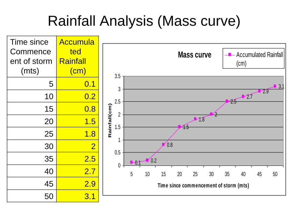
Time since

Commence

ent of storm

(mts)

Accumula

ted

Rainfall

(cm)

5 0.1

10 0.2

15 0.8

20 1.5

25 1.8

30 2

35 2.5

40 2.7

45 2.9

50 3.1

Rainfall Analysis (Mass curve)

Mass curve

0.1 0.2

0.8

1.5

1.82

2.52.7

2.93.1

0

0.5

1

1.5

2

2.5

3

3.5

5 10 15 20 25 30 35 40 45 50

Time since commencement of storm (mts)

Rain

fall(cm

)

Accumulated Rainfall

(cm)

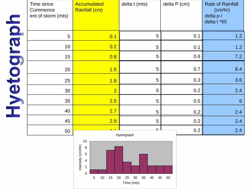
Time since

Commence

ent of storm (mts)

Accumulated

Rainfall (cm)

delta t (mts) delta P (cm) Rate of Rainfall

(cm/hr)

delta p /

delta t *60

5 0.1

10 0.2

15 0.8

20 1.5

25 1.8

30 2

35 2.5

40 2.7

45 2.9

50 3.1

5 0.1 1.2

5 0.7 8.4

5 0.3 3.6

5 0.2 2.4

5 0.5 6

5 0.2 2.4

5 0.2 2.4

5 0.2 2.4

0

2

4

6

8

10

5 10 15 20 25 30 35 40 45 50

Inte

nsity

(cm

/Hr)

Time (mts)

Hyetograph

5 0.1 1.2

5 0.6 7.2

Maximum depth –duration- Intensity curve Rainfall analysis

Time

Since

Comm

ncemet

of

stotm

(mts)

Accumul

ated

Rainfall

(cm)

Delta

T(mt)

Delta

P(cm)

Rate of

Rain

Fall

(cm/hr)

delta p/

delta t

*60

5 0.1 5 0.1 1.2

10 0.2 5 0.1 1.2

15 0.8 5 0.6 7.2

20 1.5 5 0.7 8.4

25 1.8 5 0.3 3.6

30 2 5 0.2 2.4

35 2.5 5 0.5 6

40 2.7 5 0.2 2.4

45 2.9 5 0.2 2.4

50 3.1 5 0.2 2.4

Min

Depth

cm) Max

Delta p/Delta t *60 (cm/hr)-Intensity

Maximum depth-duration precipitation(cm) of rainfall in

minutes

5 10 15 20 25 30 35 40 45 50

0.1

0.1 0.2

0.6 0.7 0.8

0.7 1.3 1.4 1.5

8.4 7.8 6.4 5.4 5.52 5 4.63 4.35 4 3.72

0.3 1 1.6 1.7 1.8

0.2 0.5 1.2 1.8 1.9 2

0.5 0.7 1 1.7 2.3 2.4 2.5

0.2 0.7 0.9 1.2 1.9 2.5 2.6 2.7

0.2 0.4 0.9 1.1 1.4 2.1 2.7 2.8 2.9

0.2 0.4 0.6 1.1 1.3 1.6 2.3 2.9 3 3.1

0.1 0.2 0.6 1.1 1.3 1.6 2.3 2.7 2.9 3.1

0.7 1.3 1.6 1.8 2.3 2.5 2.7 2.9 3 3.1

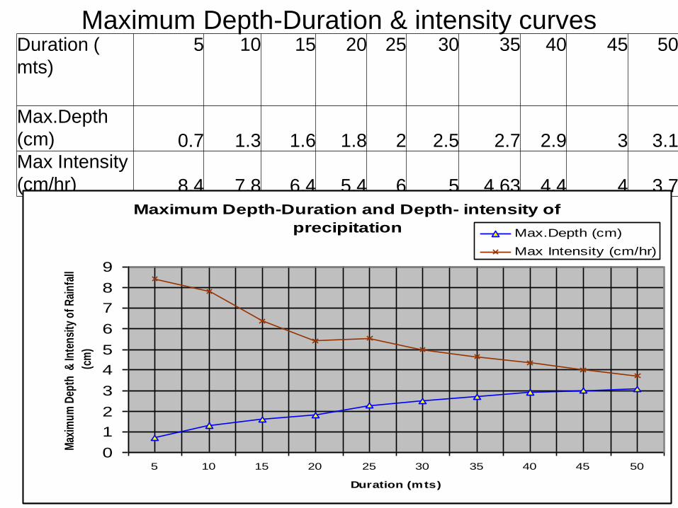
Duration (

mts)

5 10 15 20 25 30 35 40 45 50

Max.Depth

(cm) 0.7 1.3 1.6 1.8 2 2.5 2.7 2.9 3 3.1 Max Intensity

(cm/hr) 8.4 7.8 6.4 5.4 6 5 4.63 4.4 4 3.7 Maximum Depth-Duration and Depth- intensity of

precipitation

0

1

2

3

4

5

6

7

8

9

5 10 15 20 25 30 35 40 45 50

Duration (mts)

Max

imu

m D

epth

& In

ten

sity

of

Rai

nfa

ll

(cm

)

Max.Depth (cm)

Max Intensity (cm/hr)

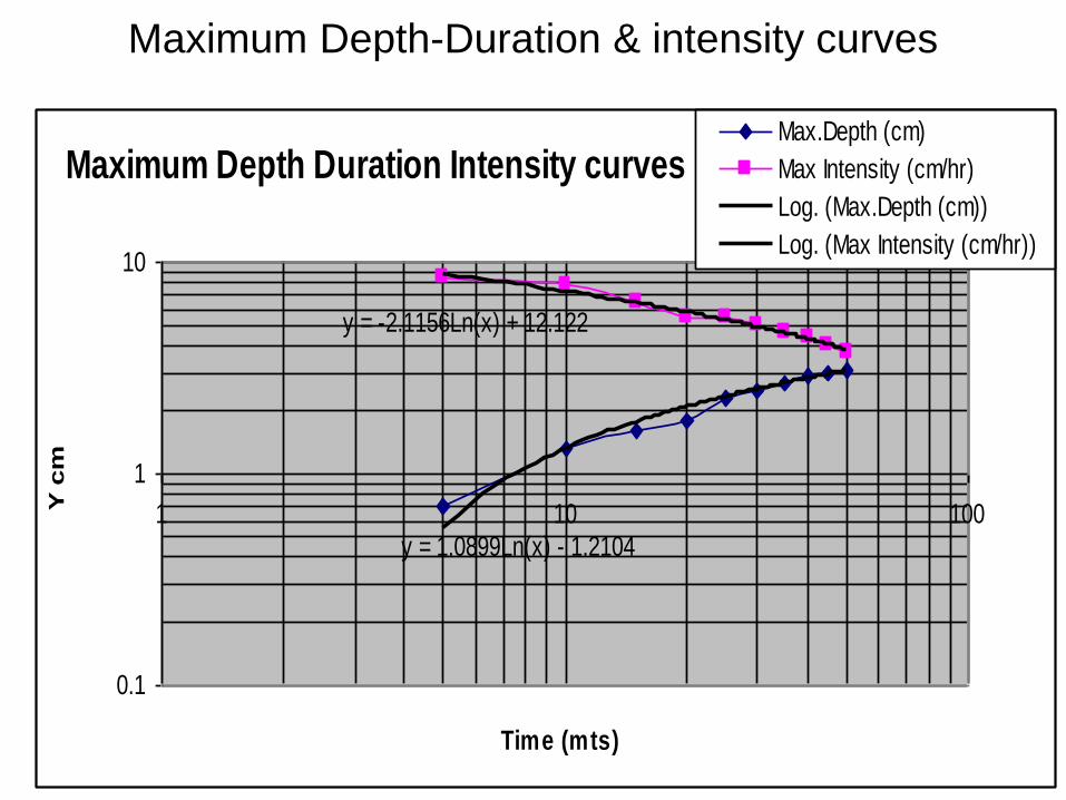
Maximum Depth-Duration & intensity curves

Maximum Depth-Duration & intensity curves

Maximum Depth Duration Intensity curves

y = 1.0899Ln(x) - 1.2104

y = -2.1156Ln(x) + 12.122

0.1

1

10

1 10 100

Time (mts)

Y c

m

Max.Depth (cm)

Max Intensity (cm/hr)

Log. (Max.Depth (cm))

Log. (Max Intensity (cm/hr))

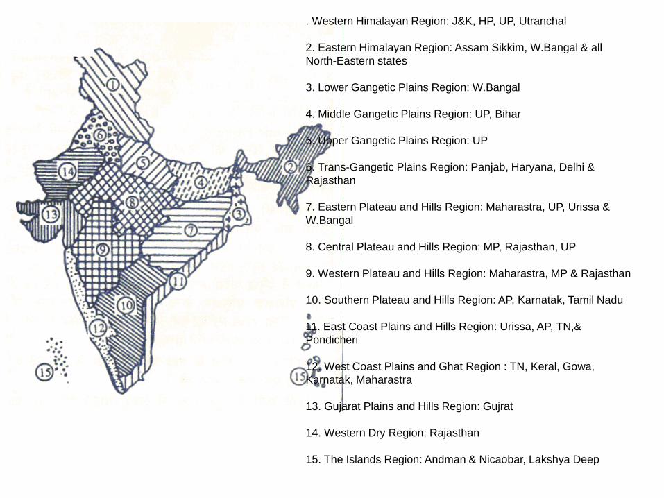
. Western Himalayan Region: J&K, HP, UP, Utranchal

2. Eastern Himalayan Region: Assam Sikkim, W.Bangal & all

North-Eastern states

3. Lower Gangetic Plains Region: W.Bangal

4. Middle Gangetic Plains Region: UP, Bihar

5. Upper Gangetic Plains Region: UP

6. Trans-Gangetic Plains Region: Panjab, Haryana, Delhi &

Rajasthan

7. Eastern Plateau and Hills Region: Maharastra, UP, Urissa &

W.Bangal

8. Central Plateau and Hills Region: MP, Rajasthan, UP

9. Western Plateau and Hills Region: Maharastra, MP & Rajasthan

10. Southern Plateau and Hills Region: AP, Karnatak, Tamil Nadu

11. East Coast Plains and Hills Region: Urissa, AP, TN,&

Pondicheri

12. West Coast Plains and Ghat Region : TN, Keral, Gowa,

Karnatak, Maharastra

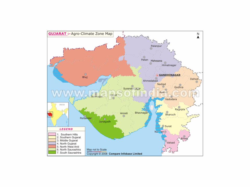
13. Gujarat Plains and Hills Region: Gujrat

14. Western Dry Region: Rajasthan

15. The Islands Region: Andman & Nicaobar, Lakshya Deep

END