pre-processing is often necessary when analyzing natural
TRANSCRIPT

AN ABSTRACT OF THE THESIS OF
Johannes B. Forrer for the degree of Master of Science in
Forest Products presented on April 14, 1987.
Title: Image Pre-processing Algorithms for Isolation
of Defects in Douglas-fir Veneer.
Abstract approved:David A. Butler
The goal of this research is to develop automatic techniques for
identifying defects in Douglas-fir veneer. To achieve this goal,
computer vision techniques, in particular image-processing, will be
applied. Several pre-processing steps may be required to enhance
images in making further analysis easier, faster, and more reliable.
Pre-processing is often necessary when analyzing natural
materials due to the amount of canplex variation present. However, if
such analysis is associated with several compute-intensive passes over
a large data set, the possibilities of what can be achieved, is very
limited.
It is advantageous to reduce the data in a way that little or no
information is lost that may affect the image analysis. This reduced
image is then used in subsequent analysis to determine the actual type
of defect, its extent and exact location. Whether such a reduction
is possible usually depends on the intended application. For Douglas-
Signature redacted for privacy.

fir veneer sheets at the plugging stage, the material is relatively
clear, with defects occupying only a minor portion of the surface. It
will be sham that reduction by pre-processing is indeed feasible.
This study investigates three potential image sweep and mark
(ISM) pre-processirg algorithms that perform this kind of reduction.
These algorithms are very diverse in their methods of operation and
include methodologies based on first-order statistics, mathematical
morphology, and color cluster analysis. It is shown in the
conclusions of this thesis that one of these algorithms is capable of
reducing the data of a typical Douglas-fir veneer image by 80% with
an error rate of only 0.3%. It is also shown that color is a
significant factor to be considered for the detection of defects.

Image Pre-processing Algorithms
for Isolation of Defects in Douglas-fir Veneer.
by
Johannes B. Forrer
A THESIS
submitted to
Oregon State University
in partial fulfillment ofthe requirements for the
degree of
Master of Science
Completed April 14, 1987
Ccarrencenent June 1987

Associate professor in Statistics/Forest Products in charge of major
limmi,W11miimilmargAAIria=..71=4 70Head of department of Forest Products
Dean of Gradua Sphool
Date thesis is presented April 14, 1987
Thesis typed by Johannes B. FOrrer
Signature redacted for privacy.
Signature redacted for privacy.
Signature redacted for privacy.

ACMIOWIEDGEMENTS
During my 18-year career, I have had the opportunity of working
with several talented colleagues, mentors, and friends who have
inspired and influenced me. My greatest rewards as a researcher has
stemmed from doing the research itself, and from the friendships I
have formed along the way. I consider it a privilege to have worked
with my committee; David 13utler, who served as major professor, James
Funck, Charles Brunner, and Thomas Dietterich, who served as minor
professor. My appreciation to Eldon Olsen for serving as graduate
council representative.
I am deeply indebted to Helmuth Resch who extended the
opportunity to work on this project, for his support, wisdom, and
friendship along the way.
Special appreciation is due to my wife Annette who provided
generous moral support and encouragement throughout the study.
(i)

TABLE OF CONTENTS
Page
Introduction 1
Literature survey 4
2.1 Introduction to the literature survey 4
2.2 Human vision, color perception andmachine perception 5
2.3 Color theory and measurement 9
2.4 The color of wood 19
2.5 Optical analysis of wood surfaces 23
2.6 Image-processing concepts 29
2.7 Summary of the literature survey 33
Veneer, its features and a proposed automatic plugger 35
The interrelationships of size-related parameters 42
Rationale and background for methodologyapplied in this study 44
5.1 Digital measures of first-orderprobabilistic differences 44
5.2 Mathematical morphology measures 45
5.3 Color clustering technique 48
5.4 Considerations for the decision rulein the mark phase 50
Algorithm evaluation 54
Dcperimental procedures 59
7.1 Experimental setup 59
7.1.1 Lighting and optics 59

7.1.2 The camera 60
7.1.3 The image digitizer 60
7.1.4 Calibration and equalization 61
7.1.5 Microcomputer 62
7.2 EXperimental results 62
7.3 A, note on the interpretation ofthe graphical material 65
7.4 Detailed analysis of SISM on three typical images 68
7.5 Detailed analysis of MISM on three typical images 70
7.6 Detailed analysis of CISM on three typical images 73
7.7 Analysis of the ISM algorithms on alarger test set 78
Considerations for tuning the algorithms 81
8.1 TUning SISM 81
8.2 Tuning MISM 85
8.3 TUning CISM 86
Summary and discussion 90
Figures 94
10.1 Preface to the figures 94
Plates 127
Bibliography 133
Appendix 139

LIST OF FIGURES
Page
Tr-stimulus values of C.I.E. spectral primariesrequired to match unit energy throughout thevisible spectrum
C.I.E. standard observers' chromaticity chart. 95
A method for evaluating minimmt image resolution. 96
Mean values for (a) intensity and(b) color for OPENEN1. 97
Variance values for (a) intensity and(b) color for OPENKN1. 98
Skewness values for (a) intensity and(b) color for OPENKN1. 99
Kurtosis values for (a) intensity and(b) color for OPENEN1. 100
Mean values for (a) intensity and(b) color for CLEAR7. 101
Variance values for (a) intensity and(b) color for CLEAR7. 102
Skewness values for (a) intensity and(b) color for CLEAR7. 103
Kurtosis values for (a) intensity and(b) color for CLEAR7. 104
Man values for (a) intensity and(b) color for PTTPOC1. 105
Variance values for (a) intensity and(b) color for PTTPOC1. 106
Skewness values for (a) intensity and(b) color for PTTPOC1. 107
Kurtosis values for (a) intensity and(b) color for PTTPOC1. 108
Results of SISM applied to (a) PTTPOC1,(b) CLEAR7, and (c) OPENKN1. 109
95
(iv)

( v )
A progression of morphological operationsusing a line segment of varying length andorientation on OPENKN1. 110
A progression of morphological operationsusing a line segment of varying length andorientation on OPENKN1. 111
A progression of morphological operationsusing a line segment of varying length andorientation on CLE7R7. 112
A, progression of morphological operationsusing a line segment of varying length andorientation on CLEAR7. 113
18(a) . A, progression of morphological operationsusing a line segment of varying length andorientation on PTTPOC1. 114
18(b). AL progression of morphological operationsusing a line segment of varying length andorientation on PTTPOC1. 115
Results of MISM applied to OPENKN1, CLE1R7and PITPOC1. 116
Dispersion values of three test images OPENKN1,CLEAR7, and PriloCl. 117
Clustering within (a) OPENKN1, (b) CLEAR7,and (c) PITPOC1. 118
Results of CISM applied to (a) PITPOC1,(b) CLEAR7, and PITPOC1. 119
A, well-behaved case. (a) and (c) good intensity(b) and (d) poor color discrimination of anopen knot. 120
An ill-behaved case. (a) and (c) good intensity(b) and (d) poor color discrimination of apitch pocket. 122

(vi)
An ill-behaved case. (a), (c) and (d) poorintensity and color, (b) marginal color responsefor a pitch streak. 124
Joint probability threshold selection for(a) a well-behaved case, (b) an ill-behaved case 126

(vii)
LIST OF TABLES
A summary of possible gross defectsPage
on a veneer surface. 36
Defects and their relationship to plywoodproduction. 37
A proposed plugging operation. 38
4(a). Relating size to image resolution.512 pixels per row resolution. 42
4(b) . 256 pixels per raw resolution. 42
Set of binary structuring elements for MISM. 47
Definition of the confusion matrix. 56
Example of an 8 x 8 binary image output by an ISM. 57
Example confusion matrix. 58
Eigenvalues and Eigenvectors for the test images. 65
Summary of clear and defect detectingaccuracies for the test images using SISM. 69
Summary of clear and defect detectingaccuracies for the test images using MISM. 72
Core vector values for the three test images. 76
Summary of clear and defect detectingaccuracies for the test images using CISM. 77
Summary of results of SISM, MISM andCIS)! on OPENEN1, CLEAR7 and P1TPOC1. 77
Comparative results of SISM, MISM, andCISM applied to three common defectsof Douglas-fir veneer. (a) Open knots,(b) Closed knots, (c) Pitch pockets. 79
Results of tuned SISM on OPENKtil, CLEAR7,and PITPOC1. 83
Results of tuned SISM applied to three commondefects of Douglas-fir veneer surfaces. 84

Results of tuned CISM applied to three commondefects of Douglas-fir veneer surfaces. 88
Summarized results of the (a) untuned and(b) tuned versions of the ISM algorithms onthe three common defects of Douglas-fir veneer. 89

LIST OF PLATES
Page
OPENKN1 127
CLEAR7 127
PITPOC1 127
SISM on OPENKN1 128
SISM on CLEAR7 128
SISM on PITPOC1 128
MISM on OPENKN1 129
MISM on CLEAR7 129
MISM on PITMC1 129
CISM on OPENEN1 130
U. asm on CLEAR7 130
CISIvI on PITPOC1 130
Tuned SISM on OPENKN1 131
Tuned SISM on CLEAR7 131
Tuned SISM on PITPOC1 131
Tuned CISM on OPENKN1 132
Tuned CISM on CLEAR7 132
Tuned CISM on PITPOC1 132

PREFACE
Machine vision, or optical-scanning technology, as it is
popularly called in forest products, has become one of the fastest-
growing high technology applications in this industry. It allows non-
contact optical measurement to be integrated into product
manufacturing. This technology makes use of visible light, very
similarly to human vision. However, machine vision cannot be equated
to human vision, even in its most sophisticated form Humans consider
vision as being "easy". As Cherniak and McDermott Gm! explain it:
"...sight is our most impressive sense. It gives us, withoutconscious effort, detailed information about the shape of theworld around us. It is also the most intensely studied sense inAl, and a natural place to begin our study of the transduction ofphysical phencanena into internal representation."
This thesis research is part of a research effort to develop
automatic techniques, using machine vision, to identify defects in
Douglas-fir veneer. It will be sham that this field is highly inter-
disciplinary, relying on the physics of lighting and optics,
mathematical statistics, computer science, artificial intelligence
(Al), and special computer architectures.
Machine vision is a relatively new field. Work that started in
the early 1960's at M.I.T and Stanford Research Institute (now SRI
International) has gained 'tremendous popularity. As is typical of a
new field, the literature is very diverse and is distributed over many
(x)

Many applications for machine vision exist in the manufacture of
veneer, plywood and lumber. Also, there are unexplored possibilities
in the development of new materials, for example, reconstituted
materials where esthetic and other visual features are important.
Numerous applications are possible in quality control, especially
veneer and particle board manufacturing.
However, several obstacles need to be overcome. First, there is
a limited source of useful literature on the optical properties of
wood. Only preliminary results of research on machine vision in wood
products exist. Thus, of the wealth of applicable ideas for image
processing, very little has been tried aix1 tested.
Second, the state of the art of image processing and analysis is
closely linked to the state of the art of the computer industry.
Applications may have to deal with grading veneer at 120 feet/minute,
or patching panels in 30 seconds. The development of parallel
architectures and associated languages and operating systems may well
be necessary before production systems for such applications are
possible.
Third is the question of perception, which deals with what is
understood after the basic image processing is completed. This
concept has been studied intensely by psychologists and researchers in
artificial intelligence. Only very simple scenes can be successfully
perceived with the present Al methods. This is indeed a very complex
and difficult subject, as it often deals with psychophysical phenomena
such as transparency, optical flow, depth and stereo vision. Barrow

(1978) concludes that
II... despite considerable progress in recent years, ourunderstanding of the principles underlying visual perceptionremains primitive. Attempts to construct computer models forthe interpretation of arbitrary scenes have resulted in suchpoor performance, limited range of abilities, and inflexibilitythat, were it not for the human existence proof, we might havebeen tempted long ago to conclude that high-performance,general-purpose vision is impossible."
This thesis shows sane important pre-processing concepts. These
reduce redundant image data without loss of information. It is
evident that several such processes in conjunction with higher-order
analysis will be required to make a useful system for automatic
inspection of Douglas-fir veneer surfaces.

Image Pre-processing Algorithms
for Isolation of Defects in Douglas-fir Veneer.
1. INTROEUCTION
Image processing deals with processes that either enhance desired
features of images or reduce extraneous information in them. It is an
important precursor to image analysis, where inferences about an image
are made. Due to the amount of natural variation associated with
images of biological materials, as well as their complexity, it is
likely that several image-processing steps will precede image
analysis. One may view this as a series of steps, each reducing
detail at its level and building towards a more complete
understanding of the canplex taAk. This observation is particularly
true for wood surfaces, where anatomical differences between species,
within species, and within samples introduce considerable variability.
Wood machining processes further introduce surface optical properties
which may affect the outcome of image processing and analysis.
Machine vision is based on the acquisition of digital images and
the manipulation of the resultant digital image data. For this study,
an image is typically made up of a 512 x 512 square array of pixels,
each consisting of three five-bit components corresponding to the
primary colors red, green and blue. Such an arrangement allows an
image to span 262,144 pixels, each capable of displaying 32,768 unique
colors. This allows the processing and analysis of high quality color

2
images.
Unfortunately, image processing is inherently compute intensive,
as it has to deal with a large amount of data. The size of the datadomain has a direct relation to the computational demands. If thesize of the data domain can be reduced in a manner that conserves
essential information, this may lead to significant savings inccartputation time. Whether such a reduction is possible depends on the
material and the intended application.
This study concentrates on Douglas-fir veneer sheets at theplugging stage, hawever the principles that are developed here may be
applied in other forest products applications. Veneer at the plugging
stage is relatively clear, with defects occupying only a minor portion
of the surface. Any image processing will thus expend a great dealof time on defect-free material. If the defect-free material can beexcluded at an early stage in the analysis, the computational demands
will be reduced significantly.
This study will follow a formal procedure. This will be toidentify, from the basic image data, the essential information-carrying channels. Then, using an empirical approach, apply a prioriinformatics.' to study the behavior of the information-carrying channels
within different contextual models. These contextual models are
derived by applying image sweep and mark (ISM) algorithms. These
algorithms are very diverse in their methods of operation, and include
methodologies based on first-order statistics, mathematical
morphology, and color cluster analysis. These three types of ISM

3
algorithms will be referred to as statistical image sweep and mark
(SISM), morpholcgical image sweep and mark (MISM), and color (cluster)
image sweep and mark (CISM).
A step common to all these algorithms is to divide the image
into a number of disjoint rectangles and then, after analysis, to mark
those which possibly contain defects. This is a two-stage process,
the first being a sweep of each rectangle in the image to analyze it,
and the second the marking. The ISM algorithms produce "low
resolution" images where each "pixel" corresponds to a rectangle
spanning several pixels of the original image. The lag-resolution
image pixels may be considered "macro pixels" and may be used in
addition to the original image for subsequent analysis.

2 . LITERAIURE SURVEY
The purpose of this literature survey was to obtain relevant
information on machine vision methodology useful for developing the
ISM algorithms. It was necessary to consider literature from several
related disciplines due to the diverse nature of the information
required.
2.1 INTROCUCTION '10 THE LITERATI.IRE SURVEY
As machine vision attempts to imitate human vision in tasks
traditionally performed by humans, some important aspects of human
vision were first investigated. This included color vision which is
believed to be important for the successful analysis of images of
Douglas-fir veneer.
Color theory presents several competing models. It was
therefore worth canparing these different models in an attempt to find
a model that offers the best possibilities for locating defects.
The forest products literature was next surveyed for insight on
how the color of wood is described and further to determine the state
of the art of "scanning for defects" of wood. This was a very limited
source in contrast with the wealth of ideas dealing with all aspects
of image processing which were found in the literature of Al, pattern
recognition, and several other disciplines.
4

2.2 HUMAN VISION, COLOR PERCEPTION, AND MACHINE PERCEPTION
Machine vision attempts to imitate human vision, however only to
a very limited extent. It is useful to briefly look at some of the
main aspects of human vision to gain soma insight of its capabilities.
Judd and Wysecki (1963) give an excellent introduction to human
vision. They state that
II... for there is a chemical as well as a physical basis forcolor. 13ut color, itself, is not purely physical or purely psy-chological. It is the evaluation of the radiant energy(physics) in terms that correlate with visual perception(psychology). This evaluation rests squarely on the propertiesof the human eye".
The human eye contains roughly 100 million receptor elements
consisting of so-called "cones" and "rods". The cones (roughly 7
million) can detect chromatic color. The cones are the receptors for
what is referred to as "photopic" vision and their profusion is
greatest where the bulk of images are formed, i.e., in the area near
the center of the retina, known as the fovea. The outer edges of the
retina are sparsely populated with cones. Rods, the other type of
receptors, complenent the cones, and function mainly in law lighting
levels for night vision. This kind of vision is referred to as
"scotopic" vision. Its sensitivity is maximal at 510 nm (green) and
yields only achromatic vision.
The human vision apparatus differs drastically from equipment
presently employed in machine vision. A major aspect is that each
5

6
cone has a direct nerve connection to the cortex, while TV cameras as
used for machine vision applications use a technique where the image
is scanned and serialized for transmission over a carrier to its
remote receiving apparatus. Even when compared with "high
resolution" TV images, the superior resolution of the human eye cannot
be matched. The apparent ease with which humans deal with very
complex vision tasks can be contrasted with the difficulty that is
experienced when attempting to use machine vision on relatively simple
tasks. This difficulty may be attributed in part to the limited
resolution of the present sensor technology.
Besides perceiving detail about the shapes of objects, human
color recognition is a fundamental faculty. This is made possible by
the presence of three different color-sensitive receptors. Baldwin
(1984) describes this color recognition process as not being the
mixture of intensities taken by the different color receptors, but
rather, a comparison of intensities. He further postulates that this
comparison is made via field arithmetic performed by the retina and
the cortex.
Presently, all grading decisions in the wood processing industry
rely on human vision. The eye provides a human operator the ability
to recognize and classify an infinite set of objects of varying color,
shape and texture. Machine vision has to compete with this
performance, which is a formidable task.
Closely associated with the vision process is perception, which
deals with image interpretation. Perception has been studied

7
extensively by psychologists and recently by researchers in
artificial intelligence (Al). Marr (1982) makes use of the concept of
the primal sketch in an attempt to describe image perception. The
primal sketch is in essence a collection of primitive symbols which,
when used within context, describes the meaning of an image. The re-
nowned artist Picasso used the primal sketch, which supposedly conveys
abstract expression.
Marr postulates that the imaging process is actually a
transformation of a three-dimensional scene to a two-dimensional
representation. Image perception has to reverse this transformation,
starting out from the two-dimensional representation and eventually
deriving an independent understanding of the meaning of the objects of
the three-dimensional world. This is no easy process as very
important information is lost in the three-dimensional to two-
dimensional transformation.
Marr subsequently suggests that in order to understand an image,
the image needs to be described as object-centered rather than viewer-
centered. This means that the viewer's perspective of an image needs
to be translated to descriptions of the actual objects. This work of
Marr was mainly developed for the perception of a three-dimensional
world. Wood surfaces haaever, are two-dimensional. Marr's ideas are
still very applicable here as they provide a foundation for early
vision processes.
Veneer and lumber are manufactured from logs which are three-
dimensional in their natural state. In the case of lumber, we may

8
consider a board as a two-dimensional image of a piece of the log. It
becanes rather important to realize that a lot of the interpretation
of defects or other features present on a board are manifestations of
three-dimensional effects and as such must be interpreted within that
context.
According to Marr's theory, the logical steps for deriving an
object centered perspective from a viewer-centered perspective,
include the acquisition of an intensity map and the derivation of
edge segments (called "edgelets") by application of edge-extraction
techniques. Marr further describes the construction of the primal
sketch using this collection of edges. Perception by means of the
primal sketch relies heavily on contextual relationships. Context in
this sense relates to how objects within an image interrelate to other
features. The optical properties of wood surfaces are rich in
contextual content such as wood grain. A knothole for instance may be
identified by recognizing its difference in texture from the
surroundirxi clear wood grain.
Although this thesis does not attempt to construct the primal
sketch, it is important to realize that the ISM operations are
considered part of the operators to derive the primal sketch.
In summary, the literature indicated the dramatic difference
between human and machine vision. With this understanding, the type
of application suitable for machine vision can be brought into
perspective. We further realize that image perception consists of
several processing steps. The primitive steps are known as "early

He further states
9
vision" or first-order processing and are of particular interest for
application in the ISM algorithms. Finally, image perception is
heavily dependent on context-related operations rather than just a few
brute-force operations.
2.3 COLOR THEORY AND MEASUREMENT
The ISM algorithms analyze features which typically describe
images. In this thesis, it is realized that the use of color
information is important. The literature offers a diverse set of
color models arrl it is essential to use a model that makes best use
of the information provided by color.
The different color models are often related by simple
relationships which are used very loosely in the different disciplines
considered in this literature survey. Let us briefly review some
aspects of the classical color models to gain some insight in what
they rnean and hcw to translate between them.
Baldwin (1984) describes some of the fundamental problems
associated with color models:
"...Color is not well understood. Whether from the standpoint ofpsychological effect, electrochemical reaction of the visualsystem, the eye's ability to match color, or the mapping ofcolor agents to color effects, there is currently nocomprehensive color theory".

10
"...a desirable theory is one that would at least permit anexplanation of the color phenomena in perceptual terms,distinctions between perceptual and descriptive models, and thematching of colors between media" .
Such methodology requires the ccfnparison of an unknown color to
a set of standards in a controlled environment (e.g. using aphotospectrcaneter) or the detection of the three basic components red,
green, and blue (R-G-B). In an attempt to create a pigment-matching
methodology so that the color range perceived by humans might be
depicted and understood, the Conanission Internationale de l'Eclairage(C.I.E.) began work in the 1920's. In 1931 the C.I.E. defined thefamous tri-stimulus standard consisting of three monochromatic
primaries red (R), green (G), and blue (B) for a "standard observer".
Figure 1(1) presents the relationship between these. The units of the
tri -stimulus values are defined such that R, G, and B are equal when
matching an equal-energy white (i.e., a light having equal energy atevery color in the visible spectrum). It is also common tonormalize the R-G-B coordinates to produce the r-g-b space
r = 12/(R + G + B),
g = G/(R + G + B),
b = B/(R + G + B) .
The definition of a color is thus defined by reference to the
illuminant and for this purpose, the C.I.E defined three standard
light sources, A, B, C. These light sources simulate cannon lighting

11
situations, such as indoor light, noon sun, and normal daylight. One
difficulty with the C.I.E. standard is that some colorimetric
calculations may yield negative tri-stimulus values, which limits
practical application. For this reason, the C.I.E defined a new
coordinate system which tploys three purely imaginary primaries X, Y,
Z such that the chromaticity coordinates X, Y, and Z are nonnegative
for any real stimulus. Z (e.g., measured in candellas/sq.cm)
represents only luminous units. A normalization procedure is done to
produce the common x-y-z coordinates
x = X/(X + Y + Z),
y = Y/(X + Y + Z),
z = Z/(X + Y + Z),
or z = 1 - x - y.
Note that the color black (X=Y=--Z) is not defined in this system.
The (x,y) chromaticity diagram results from projecting onto the
z=0 plane. A color is a point in this (x,y) space. Figure 1(b)
presents the C.I.E. standard observer's chromaticity values on the x-
y-z coordinate system. This coordinate system defines dominant
wavelength as the point on the chromaticity chart where a line
connecting the x-y coordinates of the reflected light (C), and the
illuminant's coordinates (M), intercepts the standard observer's range
(D) . The purity of the color is computed by the ratio of lengths of

12
the Um segnents MC/MD.
Pratt (1978) sununarizes several transformations between colormodels. He also provides some further definition of C.I.E.-derived
color mcdels such as the uniform chromaticity scale coordinate system
(U-C-S) which is particularly suited for the detection of subtle coloredges. For such subtleties it is desirable to use a color space that
would emphasize a color shift The X-Y-Z system is not suitable for
optimal detection of such changes because the human viewer is most
sensitive to color shifts in the blue, moderately sensitive to shifts
in red, and least sensitive to shifts in green. In 1960 the C.I.E.
adopted the U-C-S system in which equal changes in the chromaticity
coordinates result in just noticeable changes in hue and saturation.
This transformation is as follows:
u = 4x/(-2x + 12y + 3)
v = 6y/(-2x + 12y + 3)
An extension to this system is the U*-V*-W* system in which unit
shifts in both luminance and chrominance are uniformly perceptible.
This brings into account the u and v values of a reference illuminant(u0 and v0).
U* = 13 W* (u - u0)
V* = 13 W* (v - v0)

W* = 25 (100*Y)1/3 - 17.
The C.I.E. color system and its derivatives are particularlyimportant for 'TV and canputer-hardware applications.
Another coordinate system that is particularly useful for coloredge detection is the L-a-b system. This system has been used by some
researchers to report the color of wood, hag/ever it does not offer any
advantages or accuracy over the C.I.E. system. The relations forderiving the Ir-a-b units are:
L = 25 * (100 * Y/Y0)V3 - 16
a = 500 * [ (X/X0)1/3 - (y/Y0)1/3 ]
b = 200 * [ (X/Y0)1/3 - (Z/Z0)1/3 ]
where X0, YO and ZO are the tri-stimulus values for a white reference.
Colorimeters are often calibrated in L-a-b units and arecommonly used in the food processing industry. Brauner and Loos
(1968) and Moslemi (1969) reported the Tra-b values of wood when they
described the color of wood.
One practical reality of working with color-processing hardware
is that it is often easier to work with internal representations which
may appear non-intuitive to humans. Baldwin (1984) describes some of
these alternatives in color terminology used primarily in computer
graphics and printing work. The R-G-B additive primaries define a
13

14
color mixing procedure where mixing of equal amounts of red, green,
and blue produces white. Computer applications use this system
internally due to its simplicity of implementation. However, such an
additive primary system is non-intuitive to humans.
Due to the non-intuitive nature of the R-G-B color space,
especially for printing, film, and paint, a set of secondary-
subtractive primaries are derived frau the R-G-B space. By adding red
and green in the R-G-B space, yellow is produced. Similarly, adding
blue and green produces cyan, and adding red and blue produces
magenta. Cyan, magenta and yellow are the secondary-subtractive
primaries.
The use of hue, value, and saturation (H-V-S) is often used to
describe relative color measures. In defining H-V-S, the R-G-B space
may be viewed as a color cube with corners red (1,0,0), green (0,1,0),
blue (0,0,1), cyan (0,1,1), magenta (1,0,1), yellow (1,1,0), black
(0,0,0) and white (1,1,1). If the cube is viewed through an axis
between white and black, the projected shape will appear as a hexagon
with the primaries and secondaries at its vertices. The secondary-
subtractive primaries can be mixed, e.g. by overlaying colored gels:
magenta mixed with yellow produces orange and a mix of all three gives
black. This system is used extensively in the color printing industry.
Hue (H) is defined arbitrarily starting fran red at zero degrees and
progressing counterclockwise toward yellow (60 degrees), green (120
degrees) etc. This roughly corresponds to dominant wavelength. The
value (V) of a color is the distance along the black-white axis, black

15
being = 0 and white = 1. This parameter is similar to contrast in that
it limits the magnitude of the primaries. Saturation (S) is the purity
of the color as compared to the maximum purity, this is the distance
from the value axis (black-white line) towards the edge of the
hexcone. Along the black-white axis only achromatic colors (shades of
gray) exist, while pure hues exist along those edges of the hexcone
where S=1. Some of these relations are also defined by Ito and
Fukushima (1976) in their color segmentation research. These
relations are as follcws:
Intensity = R + G + B
Hue = arccos ((2r - g -b)/
(6*((r - 1/3)2 + (g 1/3) 2 + v3)2)))1/2
Saturation = 1 - 3 min {r,g,b)
where r,g b are the normalized R-C-B values.
Baldwin (1984) describes the use of intensity, hue, and
saturation (I-H-S) which follows a similar definition than H-V-S.
The following useful procedure may be used to derive I-H-S fram R-G-B
values.
Max = max( R, G, B)
Min = min( R, G, B)
d = Max - Min
V = Max

S = d/Max
r = (Max - R)/d
g = (Max - G)/d
b = (Max - B)/d
if R = Max, set h = b-g
if G = Max, set h = r-b + 2
if B = Max, set h = g-r + 4
if 11<0, set H = 60*h + 360
if h>0, set H = 60*h
Commercial television transnission needs an intensity or "black
and white" component for black-and-white television sets while still
spanning the color space. The national television systems committee
(N.T.S.C.) defined the I-Y-Q model for the transmission of television.
In this model, Y conveys the same information as Y in the C.I.E., i.e.
There also exists an N.T.S.0 model for color reception that
16
luminosity. These relations are as follc:ms:
0.60R -0.28G -0.32B
Q = 0.21R -0.52G +0.31B
Y 0.30R +0.59G +0.11B
or the inverse
R = 1.00Y +0.9561 +0.621Q
G = 1.00Y -0.2721 -0.647Q
B = 1.00Y -1.1061 +1.703Q

17
accounts for the characteristics of the phosphorous materials used in
displays.
17p to this stage of this literature survey, it was realized that
any of the color models defined thus far could have potential use.
However, Ohta et al. (1980) provide some useful information that
enables a qualitative comparison of color models to be made. Ohta et
al. used the Karhunen-Loeve (K-L) transform on the R-G-B color space
to construct an optimum set of color measures and then tested these
against r-g-b, I-Q-Y and I-H-S. The testing method was based on how
well an image could be divided into a number of distinct regions using
a particular color measure. This segrnentation procedure is described
by Ohlander (1975). Ohta et al. found two interesting results.
First, the K-L transform indicated that a nearly optimal set is
roughly:
most important measure (R+G+B)/3
second-most important measure (R-B)/2
third-most important measure (2G-R-B)/4
Second the ratios of R,G and B for the nest important Treasure are
very common for natural scenes. (1/3 1/3 1/3). The first term
(R+G-I-B)/3 , which will be referred to as the "intensity channel",
provides mostly contrast information and is what a gray-scale system
would produce. The second term, (R-B)/2, which will be referred to as
the "color channel", carries sane useful color information while the

18
last term (2G-R-B)/4 appears not to contribute much, if any, useful
information. We may consider this two-dirnen.sional nature of the color
of wood surfaces as characteristic. This analysis thus gives an
indication of the additional value of color information over a gray-
scale system. These measures are used extensively in this study.
Conners et al. (1985) researching the use of color filters for ana-
lyzing wood surfaces, favored the combination of grayscale and three
primary filters (red, green, and blue) as measures.
Spatial clustering is another important feature. We know, for
example, that knots are made up of brown colored clusters, while pitch
is yellow-brown clusters. Modelling the clustering of color enabled
Ito and Rikushima (1976) and Rikada (1978) to describe a technique for
color segmentation based on the determination of "core vectors"
(clustered feature vectors). This technique may have possibilities
and will be tested in this study.
This literature survey gives an impression that the choice of a
color model may be confusing. It is also clear that each model has
some application area where it works well. When describing natural
color scenes, the C.I.E. system works well. Using the C.I.E. system
to describe wood on the other hand, produces poor results. This is
due to the limited resolution offered to describe such monotone
subjects as wood. The paper of Ohta provides a foundation for
deriving near-optimal information channels. Extensive use of his
methodology will be made in the development of the algorithms.

2.4 THE COLOR OF WOOD
It was essential to study the forest products literature to gain
some insight on how the color of wood has been measured and used.
This part of the literature is not extensive, as the fundamental
spectral properties of wood have yet to be explored. However, some
very useful literature was found which is worth discussing.
Moon and Spencer (1948) used the (C.I.E) measures to quantify
natural wood color, which had previously only been described in
qualitative terns, such as "light reddish brawn" or "yellowish gray".
They also developed general equations using the intensity of reflected
light at three spectral frequencies which they postulated to
adequately describe the spectral reflectance curve for each wood.
Gray (1961) determined the same measures for sixteen species using
each of three C.I.E. standard light sources (A, B, and C). This
approximation of the optical spectral reflectance is rather crude, but
shows sane practical use for the C.I.E. measures. It is not clear how
useful such an approximation with only three points may be.
Sane further use of the C.I.E. measures was presented by Sullivan
(1967, 1967b). He found that for yellow poplar (Liriodendron
tulipifera) and black cherry (Prunus serotina Ehrh.), regardless of
orientation, as moisture content decreased, brightness also increased,
color purity decreased bit dominant wavelength remained the same. An
ultraviolet filter was found to increase purity but to decrease
brightness.
19

20
This similarity of dominant wavelength of wood surfaces is one
of the problems that needs to be overcame when scanning wood surfaces.
It is not uncommon for wood surfaces to appear very monochromatic
(i.e., to have the energy distribution of the reflected light be very
biased at a particular wavelength).
The way the color of wood is perceived appears to depend on three
main characteristics: dominant wavelength, brightness, and purity.
These three characteristics, in turn, are affected by the properties
of the surface i.e., color, grain, roughness, moisture content, and
orientation. The type and angle of the illumination used, the type and
angle of the detection system used, and whether any filtering or
distortion of the reflected energy occurs further affects the observed
image.
Lakatosh (1966) measured some important characteristics of wood
color: dominant wavelength, purity, luminance, and chromaticity. He
reported some typical values for clearwood, knots, decay and other
defects for a number of species. The published work of Lakatosh
showed that differences in optical properties are not in dominant
wavelength, but in intensity and purity. This work of Lakatosh is
cited extensively, hcwever it is out-dated material which used very
crude instrumentation and should be interpreted with care.
Conners et al. (1985) found that for maple, the variation in
color from one defect to another, the variation in the color between
defects and clear wood, and the variation in the color between
heartwood and sapwood occurs predominantly in only two color

21
coordinates i.e., purity and luminance, with differences in dominant
wavelength being minimal. They concluded that luminance and tonal
data can be used to separate clear wood from potential defects, but
that tonal data alone will probably not be able to differentiate among
the different types of defects.
McGinnes (1975) conducted further investigations into the effects
of filters and the type of light source on the light reflectance
properties of eastern red cedar (Juniperus Virginiana L.) and black
walnut heartwood (Juglans nigra). He concluded that fluorescent
light is less useful as an illuminant than incandescent light.
Ultraviolet and infrared absorbing filters were also shown to
significantly affect the light reflectance characteristics.
Other researchers have reported C.I.E. values for additional
species as part of investigations of wood subject to various
treatments. Most of these studies used the standard C.I.E light
source C to determine the color values. Shibamoto, et al. (1961a &
1961b) investigated the color changes due to weathering of
preservative-treated Japanese cedar (Cryptommeria japonica D.DON.) and
bamboo (Phyllostachys edulis Riv.). Brawler and Loos (1968)
investigated the color changes in black walnut sapwood exposed to heat
and/or moisture, and compared it to black walnut heartwood. They
reported small differences in dominant wavelength (575 - 580 nm).
However, significant differences in lightness (measured in L-a-b
units) and purity (measured in C.I.E units expressed as percentages)
were observed.

22
Research shading the color differences between different surface
features of the same species is of great value when doing image
processing. A limited amount of work has been done in this area,
mostly with earlywood and latewood comparisons. Moslemi (1969)
reported on the color of loblolly pine (Pinus taeda L.) before and
after exposure to sunlight using C.I.E. standard light sources A and
C. He reported C.I.E x-y-z and Lie-b color values. Exposure changed
earlywood color, however no significant change was found in latewood.
The change in earlywood color is frau yellow (approximately a = 0, b =
25) to purplish-blue (approximately a = 10, b = -5). Resch et al.
(1968) reported that the color difference between incense cedar
(Libocedrus decurrens Torrey) sapwocd and heartwocd was not sufficient
to be used for segregation purposes in a drying study of pencil stock.
Nelson et al. (1969) investigated the relationship of black walnut
heartwood color to site, soil properties, and geographic location,
using C.I.E light source A. Webb and Sullivan (1964) investigated
the color changes due to the exposure of wood surfaces to carbon-arc
light and water on redwood (Sequoia sempervirens) and Engelman spruce
(Picea engelmannii). They found no change of color between spruce
earlywood and latewood due to the treatment. Redwood also showed no
difference in dominant wavelength, but the latewood portion of the
annual ring was found to be brighter and to have a lower color purity.
In summary, the literature contains several papers confirming the
monotone color of wood. Its dominant wavelength is roughly 580 nm.
Its color variability is in brightness and purity. The C.I.E. tri-

23
chromatic system is widely applied, though considering the limited
range of variation in the color of wood, this system may be inadequate
for detecting defects using machine vision.
2.5 OPTICAL ANALYSIS OF WOOD SURFACES
The ultimate objective of this research is to develop the
necessary fundamental theory and algorithms to enable automated
machines to produce wood products. This is not a new idea: in fact it
is presently one of the fastest growing areas in machinery
development. This is evident when attending trade shows and when
visiting some of the modern high-efficiency wood-processing plants
around the U.S.A.
There are some useful references in the literature that cover
the early development of this technology, and others that indicate the
current state of the art.
The application of optical imaging systems for the interpretation
of surface characteristics of wood is an ambitious undertaking.
Szymani and McDonald (1981) and Szymani (1984, 1985) reviewed methods
that show potential for interpreting the surface characteristics of
lumber. These include scanning with ultrasound, x-ray radiation,
infrared light, and visible light. They concluded that no one method
distinguised itself as being capable of yielding reliable results.
However, they felt that systems emplcying visible light had certain
advantages that yield higher reliability.

24
Conners et al. (1983) described a conceptual automated lumber
processing system (ALPS) for the production of southern red oak
furniture parts. This system was designed around a gray-scale machine
vision system capable of detecting 8 common types of board defects.
The reported accuracy varied from 57.35% to 98%. The methodology
employed for this work is based on texture analysis using spatial
gray-level dependence (SGLD). It was also shown that first-order
statistical analysis had the potential for classifying clearwood with
91.67% accuracy. This then presented the idea for designing a two
stage analysis where the first-order statistical analysis would
precede a second-order statistical analysis. Using such a
hierarchical approach, a defect could be labeled with 88.33% accuracy.
This paper also alluded to the possibilities of color.
Conners et al. (1984a) and (1984b) is basically a repetition of
the 1983 paper. However, Conners et al. (1985) presented the first
attempt to utilize the color of wood. In this paper a gray-scale
system was used in conjunction with color filters. This analysis was
performed on surfaced maple samples. No comparison was made to their
earlier work on red oak. Eight different types of defects were
located, using only the first-order statistical technique. It was
shown that the red-blue combination showed better results than the
green-blue combination, except for the detection of decay. Cambining
gray-scale and values obtained through the filters (red, green and
blue) produced the best defect detection accuracy. Of further
interest in this paper was a study to analyze the performance of human

25
graders. It was fourrl that the machine vision system accuracy was as
good as those obtainable by human workers.
Soest (1984, 1985) described a system using laser scanners to
detect defects on ltnnber. This system makes use of
* anisotropic scattering and transmission of light insoftwood cells
* provides fundamental discrimination between defectiveand clear wood ".
The principle of operation is that a laser beam is focused on the
surface of the wood. Due to the anisotropic scattering of light in
sound wood, an elongated reflection pattern is observed. Defective
wood does not show this elongated pattern and is thus detectable.
Defective wood such as compression wood is nearly impossible to
detect by the naked eye. A human observer would describe such wood as
"lacking in luster", however it is very difficult to be reliably
detected. It is important to be able to detect compression wood as
such wood has inferior strength properties. The method suggested by
Soest has the ability to detect such compression wood.
Soest (1984, 1985) reports that the location accuracy for this
method is within 1 mm for face knots and within 2 mm for spike knots.
Although defects such as blue stain are sham in his examples, it is
not clear by what methodology this defect is sensed. The idea of
testirg for sound wood ultrastructure is very interesting and may gain
importance in future.

26
Mathews and Beech (1976) hold a U.S. patent on another laser
scanning technique. This technique is based on simple light
reflection properties and has not been proven successful. An
operational system was described in Wood & Wood Products (1980).
However, Conners (1983) has pointed out some deficiencies of this
system due to its reliance on only first-order differences. It is
also evident that special human intervention is required at times to
make the system work.
At the 1986 Forest Industries show in Portland, OR., Machine
Vision International (MVI) demonstrated their "image-flow" hardware,
which is based on a pipelined hardware implementation of morphology
operations, to grade veneer sheets (4 feet wide by 8 feet long) at
production speed (120 feet per minute. Although this hardware is very
advanced for the forest products industry, several important
properties of wood are overlooked. These machines have their origin
in the autarritive industry and attempts to do a simple transplant have
sham that wood surfaces are very complex to analyze. It is also not
certain whether the methodology that the machines are based upon will
work on wood.
Sate European researchers have employed machine vision in forest
products applications. Mehlhorn and Plinke (1985) described
possibilities for the use of a gray-scale system for quality control
in machinirxj solid-wood products. Arnold (1986) described a system to
measure the morphology of chips for particleboard manufacturing. Such
analysis may aid in the optimization of adhesive usage and also

27
ensure a product with tightly controlled properties. Fischer et al.
(1985), an East German research group, described optical, X-ray and
infrared imaging techniques for the detection of defects in solid
lumber. Their technology appears to lack sophistication.
Scandinavian researchers have devoted a considerable amount of
effort to scanning boards for automated board edging. Maleta Gmidescribes the Saab "Q-option" for the detection of knots, splits,
cracks, grain, pitch, stain, etc. Although the system is designed for
edging, grade plays part of the edging decision and thus their
interest in defect detection. An increase of 3.8% in grade recovery
was reported.
Karonen (1985) describes an edger developed by the company
Ahlstranlitich
" has developed a grade scanner from camera and visible lightbase. Knots and defects with color disparity from sound woodare detected by optical contrast This detection is supportedby micro-wave scanning, which separates knots from knotresembling stains. The final grade of a board depends on knottype, e.g. whether red och (?) black. This can be determined byinfra red light. When illuminating the board from one side byIR-light, red knots let the light pass easily through and thisis detected by another camera on the other side. "
The combination of several scanning techniques in this paper
indicates the inability of optical methods to sense internal defects.
However, without the application of color vision technology, the use
of infrared scanning and gray-scale vision seems promising.
The literature survey on optical scanning methods showed that the

28
technology for analysis of the optical properties of wood has
tremendous potential however, except for the work of Conners et al.
(1983, 1984a, 1984b, 1985), very little progress has been made towards
automatic detection of defects. One intuitive reason for this is the
complexity and diversity of the problem, as well as that a special
kind of cart:titer hardware is required. This kind of computer hardware
is presently being developed and is slowly becaming available.
Color machine vision is in its infancy. Color will be sham to be
one of the requirements for the successful detection of defects.
There further appears to be a lack of generalized methodology for
detecting defects using machine vision. The only methodology
described is by Conners et al. (1983,1984a,1984b,1985), i.e.,
statistical classification. Their use of color is not as elegant as
the work done by Ohta (1985), however it must be considered as a
"first attempt". The hierarchical processing approach described by
Conners et al. (1983) has potential and will be pursued in this
thesis.
The praaising results obtained in Scandinavia would be hard to
duplicate with species other than their light-colored spruce. Such a
light-colored species allows relatively simple technology, i.e.,
simple thresholding and ronochrome imaging, to be employed.
It thus appears that a great deal of development, both in the
development of defect detection methodology, as well as in color sci-
ence remains to be done before automatic defect detection will be
generally applied in the forest products industry.

2.6 IMAGE-PROCESSING CONCEPTS
The forest products literature covered only a very limitednumber of image-processing techniques. The literature survey was thus
expanded to include literature from other disciplines, particularly
image processing, signal processing, electrical and computerengineering, and Al and psychology. Several promising techniques were
found. Not all the cited material which follows has directapplication in this thesis research, but is included for completeness.
Historically, image processing has developed along empirical, as
well as formal lines. Darling and Joseph (1968) described the use of
threshold logic as a means of pattern recognition for applications on-
board satellites. This logic reduced an image to a set of feature
values and greatly reduced data transmission times. This idea has
future potential once the so called "artificial neural network"computer architectures becorre freely available.
A syntactic approach to image processing has been described by Lu
and Fu (1978) and Fu (1974). This is based on a picture-grammar
description of texture. Using this grammar, a binary image is parsed
for possible recognition of phrases, sentences, and other constructs
of the language described by the grammar. To compensate for
discontinuities or to recognize fuzzy pictures, a special structure-
preserving error-correcting tree automaton (ECTA) was employed. In one
of the examples in this paper, the analysis of wood grain was shown.
Kelly (1971) introduced the idea of hierarchically organized
29

30
images with different levels of resolution. Analysis in low-resolution mode provided important information which aided searching
in high-resolution mode. He achieved successful edge detection, even
with images having high noise content This concept may prove useful
during post-ISM processing, especially for the detection of defect
boundaries.
The treatment of images as stochastic processes occurs more
frequently in the literature. Several probabilistic techniques were
introduced by Haralick (1973a, 1973b). These dealt mainly withsecond-order statistics to describe texture and are Imam as spatial
gray-level dependence matrix analysis (SGLD). Conners and Harlow
(1980) and 'Weszca et al. (1976) fourd that SGID analysis were superior
to other texture-analysis methods such as power spectral methods
(using the Fourier transform), gray-level difference methods orgray-level run-length methods.
SGLD analysis is usually preceded by image enhancement in an
attempt to maximize contrast Haralick (1973) and Conners and Harlati
(1978) presented and evaluated equal-probability quantizing to perform
this contrast adjustment. This procedure =dines the image data so
that a nearly flat histogram of the gray-scale values is obtained.
However, only structural features and texture will appear enhanced,
indicating that such a procedure should be used with care for any
analysis except texture analysis. Conners et al. (1983) used this
technique prior to SGLD analysis to compensate for contrastdeficiencies. No results are shown to indicate whether or not it

31
actually produces better results, however in the earlier papers it was
shown that better results can be obtained when analyzing simulated
textures.
The objective of these statistical techniques is to extract
features which may be useful during image classification. Several
techniques for selecting an optimal set of features from a
comprehensive set are available, including Fischer discriminant
analysis, maxinann likelihood analysis, and Bayes' rule. Duda and Hart
(1973) is an excellent source of information on statistical
classifiers. Kruger et al. (1974) also describe a useful selection
methodology for obtaining an optimal feature set by eliminating
redundant features, as well as determining the features' relative
importances.
Connectivity analysis is useful when describing the hierarchical
relationships between connected parts (blobs) within images, their
sizes, orientations and shapes. Connectivity analysis has been
attributed to efforts at Stanford Research Institute (now SRI
International) and is thus also Imam as the SRI algorithm. Rosenfeld
(1970) provided rigorous mathematical proof for many of the concepts
in connectivity. An interesting paper by Ho (1983) evaluates the
accuracy of this technique. For a practical treatment of connectivity
algorithms, see Cunningham (1981). A more general approach to image
analysis, in terms of the theory of nranents, is presented by Teague
(1980) as an extension of binary connectivity to gray-scale.
Mathematical morphology, or the treatment of images as

32
topological sets, was developed in the mid 1960's by the Centre de
Morphologie Matematique of the Fontainebleau School in Paris.
Mathematical morphology, or simply "morphology", as it is popularly
known, includes a number of operators: dilate, erode, open, and
close. These operations use a structuring element that operates on
the images. The structuring elements can take on any arbitrary size
or form, and their use implies that an image may be manipulated
selectively by the shape of its objects. For a comprehensive
treatment of mathematical morphology and image analysis, see Serra
(1982). Morphology algorithms have some special properties that
make them attractive for implementation in a specialized pipelined
hardware architecture. Sternberg (1979, 1981, 1985) originally
developed this pipelined hardware for image analysis in a cytology
application.
Another application of morphology to extract textural features of
images is described by Werman and Peleg (1985). Their technique has
the ability to measure isotropy and coarseness of texture. It
applies fuzzy logic theory to Serra's morphological operators, thus
extending morphology on binary images to gray-scale. This technique
offers interesting possibilities, i.e., implementation on pipelined
processors, and is one of the techniques that will be evaluated in
this study.
It is worthwhile noting that a real application may require a
combination of several techniques, including image enhancement, edge
detection, filtering by mean or median operators, template matching,

33
table lookup methods, thresholding and segmentation, and others.
Weszca (1978) is a widely cited source on the topic of thresholding.
This paper discusses various practical threshold selection techniques.
2.7 SUMMARY OF THE LTIERATURE SURVEY
To summarize this literature survey, we need to reconsider the
objective of this thesis: to investigate potential methodology and to
develop algorithms, which, when applied to images of Douglas-fir
veneer, will reduce image canplexity. This is considered an essential
step towards the achievement of an automated veneer plugging system.
As such, these algorithms should be computationally efficient, and
should be highly reliable in focusing on potential defects.
The literature survey for this thesis was extensive. This is
indicative of the nultidisciplinary nature of the field.
Several papers confirmed the monotone color of wood. Its
dominant wavelength is roughly 580 nut; its color variability is in
brightness and purity. The C.I.E. tri-chromatic system forms a common
basis of measurement, although when considering the limited range of
variation in the color of wood, this system is inadequate. Using
Ohta's work on the derivation of an alternative color model, some
experiments done in conjunction with this thesis showed that the color
of Douglas-fir veneer surfaces is consistently two-dimensional (see
also section 7.2). This fundamental concept is applied in all three
algorithms to extract features.

34
The papers by Conners et al., suggested a first-order statistical
analysis in a hierarchically organized system. This idea provided the
basis for the SISM algorithm. It also served as a rough benchmark as
to what could be achieved. However no valid canparison between the
results of this thesis and those from Conners et al. can be made
unless SISM can be tested on the same sample set that they used.
Werman and Peleg's paper suggested a novel texture analysis
technique based on mathematical morphology. This idea provides the
basis for the MISM algorithm. Not only is texture an important
feature of wood, but morphology offers some possibilities for
implementation on specialized hardware that is presently making its
way into equipment for application in the forest products industry.
Same very useful, although originally obscure, methodology was
obtained from Fukada's paper on spatial clustering. This paper
provides the basis for the CISM algorithm.
Although the ISM algorithms are intended to perform a specific
function, in a more encompassing image analysis scheme the ideas of
Marr and his contemporaries, Barrow, Tenenbaum et al. provided
confidence that, in principle, ISM is a valid and important step. As
such, ISM may be considered a step tcmard the derivation of the primal
sketch and perhaps in a broader sense, a first-order analyzer.

3. VENEER, ITS FEATURES AND A PROPOSED AUMMATIC PLUGGER
Before going into a more rigorous description of the ISM
methodology, let us briefly consider some aspects of the veneer
production process. It is easier to understand what issues are at
stake by knowing the material and its properties better. This will
place sane of the ideas developed in the ISM in perspective and add to
the base of ideas acquired during the literature survey.
Douglas-fir veneer is created by a peeling process wherein a log
is rotated against a knife in a veneer lathe. This process creates
approximately a tangential section of wood. Its anatomy, as well as
the machining method, greatly influences the characteristics of the
surface. Table 1 gives a general summary of these properties.
Considering this table, one might assume that if tone, wood
grain, earlywood/latewood patterns, and defects could adequately be
described by mathematical models, then any arbitrary inference about
the image could be derived. However, no present methodology has yet
dealt successfully with natural scenes, even with very simple ones.
In this study, some aspects of tone and texture (as they relate to
wood grain are earlywocxl/latewood patterns), are studied. Statistical
image sweep and mark (SISM) is used to study the tonal properties
while morphological image sweep and mark (MISM) is used to study
textural properties. Color cluster image sweep and mark (CISM) is a
further study of tonal properties, however in a different context than
SISM.
35

Table 1. A summary of gross features of a veneer surface.
36
This research deals with Douglas-fir veneer at the plugging
stage. The plugging is a required step to upgrade veneer sheets for
use in the face or back for plywood construction. For example, for a
panel to be graded "A", not more than 18 neatly node repairs, of
boat, sled or router type, parallel to grain, are permitted. Defects
may occur at several of the production stages. Table 2 presents the
veneer production process and indicates the type of defect that may be
present at the different stages.
Property CommentsF
Tone Describes global properties, i.e.,mean color etc.
Wood grain Grain is due mostly to its alignedfibers. (85% axial, 15% transverse)
Earlywood/latewood Alternate bands of material densitypatterns corresponding to seasonal growth.
Due to the tangential surface,these regions form very character-istic patterns along the grain, thelatewood being of darker color.
Defects Defects are of two general types:those introduced while the tree wasstill growing, and those introducedafter logging. Defects eitheraffect the strength or appearanceor determine its value.
MOM OM

Table 2. Defects and their relationship to plywood production
1 PROCESS PROCESS TYPE OF DEFECT DEFECT TO1 DESCRIPTION DEFICIENCY INTRODUCED DETECT
CRYINGimpropersegregation(heart/sap)
shrinkagechecksdiscoloration
IMON41.4/110.110=.1111.1IMP............NII4
wet veneersurface in-activation
37
The lathe and clipper are considered the "green end" of veneer
manufacturing. Drying and plugging are considered the "dry end".
Panel lay-up and finishing forms the remainder of plywood
manufacturing. It is estimated that, under typical conditions, about
open holesloose knotstight knotspitch pockets
poor mach- Torn fibers pitch streaksPUJGGING inery bark inclusion
small burlswanesplitsstaininsect damage
-+LAY-UPSPREADPRESS
core gaps blows blowsgapsroughness
roundupCLIPPER clipping wane wane
strategy splits open knotsclosed knotsholes
roundup waneLATHE equipmnt
pre-condi-tioning
lathe checkschecks, splitsroughnessthick/thin
No defectdetection

machine vision system
A veneer unstacker loads veneer sheets onto a X-Y table. Such
table is equipped with electric motors arbd transport mechanics which
enable one to position the veneer precisely at any given coordinate
within its field of travel. Typically this positioning is controlled
by a computer for easy integration into automatic systems. The sheets
38
50% of the wood from each log ends up in plywood.
From the above table it is evident that the plugging operation
is preceded by cleanup operations, so that only cosmetic defects
remain to be removed frail face and back panels to upgrade the value of
the product. Of the 11 listed defects, knots (both open and closed)
and pitch pockets are the most frequent. Presently, this upgrading
operation is performed manually. A proposed automated plugging
operation is presented in Table 3.
Table 3. A proposed automated plugging operation.
cartputer driven punch/plugger+7.77+
I I\/veneer veneer
unstackerI 0
I stacker
> x y table
0+77777.77/ \77...omOo+

39
are then firmly clamped down and then transported under the vision
system's camera. Due to the limited field of view of the vision
system, the total sheet area will typically be divided into smaller
areas which will be analyzed in turn. For each of the areas, the
vision system inspects the area, then locates the defects and builds a
defect list. This defect list contains the type of defect and its X-Y
co-ordinates for later reference by the plugger.
After completion of inspection of the total sheet area, the
plugging operation ccurmences. The defect list is first analyzed to
consolidate smaller defects into areas which may be patched by the
same plug. Sate further decisions might include the elimination of
insignificant defects from the defect list. Using the consolidated
defect list, the sheet is graded first, because plugging has to
consider grade. Then the X-Y table is positioned under the
punch/plugging head to perform the actual plugging. Finally the sheet
is released and fed to an unstacker.
This study will only deal with sate aspects of the machine vision
process, nct the overall system. Fbrther, only the analysis of one
of the subirnages is considered as it would be simple to extend the
principles to include a succession of subimages that make up a full
sheet.
In a real production system where real-tine requirements have to
be met much more may be involved. It may need to employ multiple
cameras to be able to process larger areas of the veneer sheet in
parallel. In such applications it be necessary to implement parallel

40
processing, however this is beyond the scope of this thesis.
The image sweep and mark principle (ISM) will next be briefly
described in order to place sane of the hardware and systems software
in perspective. However for a full description of ISM please see the
sections "digital measures of first-order probabilistic differences",
"mathematical morphology measures", "color clustering techniques", and
especially "considerations for the decision rule in the mark phase".
The vision system acquires a digital representation of the
subimage through use of a "frame grabber". This electronic device
serves as the interface between the optical sensor ard the computer.
It contains high-speed analog-to-digital convertors that convert the
analog video signals frail the TV camera into digital values and store
these values into a special buffer called a "frame buffer". This
frame buffer is accessible by the system software for further
manipulation. When we refer to an "image" within the system software,
we actually refer to the representation of the image within this frame
buffer.
A two-step software analysis then follows: first, the image is
subdivided into a number of disjoint rectangles which are analyzed in
turn as the image is swept. Curing the sweep of the image rectangles,
use is made of an unsupervised learning technique which constructs
distributions of image features. The second phase then uses these
distributions to mark rectangles that differ significantly from what
is expected from the distributions.
This method is by definition global, as each marking decision is

41
made without reference to local context. However it does include
important contextual information as each mark decision considers the
contribution of each rectangle to the overall distribution.
In summary, this section expanded the scope of the literature
survey by considerirg veneer and its characteristics as it relates to
this thesis. A proposed system implementing ISM in an automated
veneer plugger was also presented.

4. THE INTERRELATIONSHIPS OF SIZE-RELATED PARAMETERS
Several factors relating to size play an important part in the
overall system performance. These are the interrelationships between
the image size, the spatial resolution and rectangle size. These
relationships are presented in Tables 4(a) and (b) for three image
sizes: 5"x3.75", 10"x7.5" and 20"x15".
Table 4(a). Relating size to resolution. 512 pixels per row
resolution.
1 image size 1 pixels/inch I rectangle sizes1 1 I 16x16 32x32 128x128
1 5"x3.75" 1 102.4 I .156"
1 10"x7.5" 1 51.2I .3125"
1 20"x15"1
25.6 1 .625"
Table 4(b). 256 pixels per raw resolution.
1 image size 1 pixels/inch 1 rectangle sizes1 1 1 8x8 16x16 64x64
1 5"x3.75" 1 51.2 1 .156" .313" 1.25"
1 10"x7.5" 1 25.6 1 .3125" .625" 2.5"
1 20"x15"1
12.8 1 .625" 1.25" 5.0"
42
VINO
.313" 1.25"
.625" 2.5"
1.25" 5.0"

43
These relationships determine the size of the smallest defect
that will be detectable. Small defects will require higher
resolution, while for larger defects lcwer resolution will be ade-
quate.
The follcming sinple parameter-evaluation procedure was performed
to tune the algorithms for veneer plugging. Other applications may
require different parameters. The purpose of such a procedure is to
optimize the resolution for a given defect size without increasing
computational complexity, i.e., to use the lowest feasible spatial
resolution and the largest feasible rectangles. This procedure is
outlined in Figure 2.
This procedure starts with an arbitrary physical image size.
Men depending on the pixel resolution required, a rectangle size is
chosen. The ISM algorithms are then used iteratively to determine
whether the rectangle size is adequate. Adjustments are carried out
until a suitable rectangle size is found. If it proves that no
suitable rectangle size works, then the image size is adjusted and the
process for evaluating rectangle size repeated.
Using this methodology, it was found that an image size of 10" x
7.5" using 256 mode and a rectangle size of 8 x 8 pixels
(0.3125"x0.3125" actual ciinension) produced acceptable results for the
type and size of the defects encountered in this study.

5. RATIONALE AND BACKGROUND FOR METHODOLOGY APPLIED IN MS STUDY
The purpose of this section is to formally present the definition
of terminology and methodology for the image sweep and mark principle.
This is divided into four sections: statistical image sweep and mark
(SISM), morphological image sweep and mark (MISM), color cluster image
sweep and mark (CISM), and considerations for the decision rule in the
mark phase.
5.1 DIGELAL MEASURES OF FTRST-ORDER PROBABILLSTIC DIFFERENCES
SISM divides the image space into n disjoint rectangles as
described by Conners (1983). For each of the n rectangles, statistics
are computed for intensity ((R+G+B)/3) and color ((R-B)/2). These
include first, second, third, and fourth order probabilistic
differences of individual pixels to describe the siniplest textural
features of images.
Let P(i) be the proportion of occurrences for level i of the
measure. Further, rescale all measures to the range (0 - 31). This
makes it possible to generate computer graphics for some of the
intermediate results as an additional diagnostic tool. This scaling
is in order as the follcwing fonnulae are adjusted for the mean. The
above statistics are then defined as:
44

MGM, M = Sumi (i*P(i) )
variance, v2 =Sum ({ i-m)2*P(i))1
skewness, s = Sunii { (i-m) 3*P(i)/v3/2)
kurtosis, k ='Sum ({ i-m) 4*P ( i) /v2 )1
The mean describes the first-order raw moment about the origin.
Variance is a measure of dispersion about the Mean. It is also a
useful measure of contrast. Skewness is a measure of asymmetry about
the mean. Kurtosis is a measure of the pointedness of the
distribution or haw heavy the tails are.
5.2 MATHEMATICAL MORPHOLOGY MEASURES
Since wood is anisotropic, it is useful to quantitatively express
directional properties of wood surfaces. As for the statistical
method, the image is divided into n disjoint rectangles. Textural
features for a given sub-image can be generated by operating on it
with different structuring elements. The function of the structuring
element in morphology is to perform shape and orientation sensitive
operations on the image data. The operations used in this thesis are
gray-level generalizations of "dilation" and "erosion" for binary
pictures using Serra's (1980) morphological methods as described by
Werman and Peleg (1985).
Let A(a) be the pixel value of the gray-scale image A at location a.
45

46
Let B(a) be the pixel value of the gray structuring element B at
location a.
Then the dilation of A, the gray-scale image A, by the gray-scale
structuring element B, is the set defined by:
DAB(a) = supb {min (A(b) ,B(b-a)) }
where b is an element of B.
When B is a binary structurirg element then
DAB(a) = sup{A(a+b))
where b is an element of B.
(sup (suprercum) means the least upper bound)
The erosion of A, the gray-scale image A, by the gray structuring
element B, is the set defined by:
E(a) = infb {max (A(b), 1-B(b-a)))
where b is an element of B.
When B is a binary structuring element then
E (a) = inf(A(a+b))AB
where b is an element of B.
(inf (infimum) means the greatest lower bound)
Utilizing color information, any appropriate color measure
(intensity, hue etc.) may be used to represent the image content.

47
Since the morphological operations are defined for single measures
only, intensity (0Z+13-1-W3) is the obvious choice as it represents
structural variation. It would be possible to include other
information channels as well, however not much is known about the
interpretation of such multidimensional morphological operations.
This was not considered viable for this thesis as the only alternative
channel, i.e., 02q/2 provides no additional structural information.
The binary structuring elements used in this thesis were chosen
in order to be able to measure texture in four directions. They
consisted of line segments of eight different lengths in four
directions. The geometry of the structuring elements are presented in
Table 5.
Table 5. Set of binary structuring elements for MISM
(135) (90) (45)
* * ** * *x* * * * * * * * (0)
(lengths 0 1 2 3 4 5 6 7 8)
To summarize the results of these morphological operations on the
image, matrices are generated, each consisting of nine rows,
corresponding to lengths (0,1,2,3,4,5,6,7,8), and four columns,

48
corresponding to directions (0,45,90,135 degrees). Each matrix
element represents the computed sum of the gray-scale values over all
pixels of the rectangle. Morphological operations that have strong
effects on the image turn the gray-scale values darker (using
dilation), thus resulting in lower summed values for the rectangle.
Morphological operations that have little effect on the image data
leave the surraned gray-scale values over the rectangle unchanged. The
way this experiment has been designed allows inferences to be made
regarding the orientation of features as well as their size.
5. 3 COLOR CUJSTERING TECHNIQUE
There have been two types of approaches to image segmentation:
differentiation, which deals with the definition of edges that
separate regions, and clustering, which locates regions directly
through similarity grouping. The latter is ccamnonly referred to as
either region splitting when iterative division of an image is
performed, or region growing when regions are built from merging
"atomic" elements. The technique used in this study is based on
clustering principles, where the euclidean distance between the color
coordinates of two pixels is the measure of similarity.
Let each pixel be denoted by a 2-dimensional vector with
elements:

xl = the value of the intensity channel (RFB+G)/3
x2 = the value of the color channel (R-B)/2
A region is then defined as a partial image of spatiallyconnected pixels whose vectors are similar. The cluster analysis
technique requires that the image be subdivided into a number of
disjoint subirnages. For each subirnage the dispersion and mean vectors
are computed as follows:
dispersion = The trace of the covariance matrix of
a rectangle.
mean vector mean of (xl,x2) over a rectangle.
Next, a set of rectangles having dispersions below a given"dispersion threshold" (i.e., a set of rectangles of relativelyuniform intensity and color) are selected. The selected rectangles
are called "core-candidates", and their mean vectors are called "core-
candidate vectors". This models prevalent color by including only
uniform regions. Next, clusters within the selected set are found.
The euclidean distance between the two core vectors that arefarthest apart indicates haw "spread-out" the distribution is, whilethe shortest distance between any two core vectors is an indication of
hag "canpact" the distribution is.
The selection of the maximum allowable number of core vectors is
important as this will influence had well odd-shaped distributions may
49

50
be modeled. The selection of the dispersion threshold will determine
haw homogeneous the set of rectangles is on which the cluster analysis
will be done. These selections are heuristic ones and" ... is based
on human intuition and experience ... " (Tou and Gonzalez (1974)).
Segmentation is then possible by classifying each rectangle into
a certain region depending on its distance from the core vectors. The
region it belongs to is that of the core vector closest to it.
However, if this distance to the closest core vector exceeds the
bounds of the model, then the rectangle is classified as "unknown".
Cluster analysis is performed by application of the ISODATA
algorithm, which is a cluster-seeking algorithm. (Duda and Hart
(1973), Tou and Gonzalez (1974)).
5.4 CONSIDERATIONS FOR THE DECISION RULE IN THE MARK PHASE
To perform the mark phase using any of the described
techniques, a test is necessary to discriminate between rectangles
containing defects and those of perfectly sourbd wood. The ALPS system
(Conners, et al. (1983)) uses a chi-square test as a goodness of fit.
This requires the use of a training set frau which a set of norms for
the features are extracted. This is applicable when the feature set
is Imam to be well-behaved. However for this study, this was not the
case, and an alternative needed to be considered.
Scene useful concepts have been derived from Bayes decision theory
for application in the testing procedure developed for this study.

51
Consider Xi (for i = 1...m), to be a member of the feature set, and
let Ck (for k = 1...L) denote a class of wood. Then
P(CkIX) (1:(X1C/c)P(C/c)/(Surni (13(XIC1)P(Ci)))
( for i = 1, ...,L )
where
P(Ckl = probability of class k given pattern X
(the a posteriori probability)
p(XICk) = probability of pattern X given class k
p(Ck) = a priori class probabilities
Bayes' rule minimizes the probability of misclassification by
choosing the the class C having maximum a posteriori probability,
P(Ckl , among all the classes considered. However, it assumes that
the a priori probabilities, p(Ck), as well as the class-conditional
probabilities, P (X 1 Ck) are known. This is seldom the case.
However, it is possible to estimate these probabilities, provided the
number of classes is known. Frequently even the number of classes is
unknown, and one has to resort to unsupervised methods i.e., those
that do dynamic estimation.
The observed variation of Douglas-fir veneer clearwood indicates
that several classes of clearwood might exist, necessitating sane form
of unsupervised methodology to determine the number of classes. Since

52
the level at which the ISM routines work should be optimized for
efficiency, Bayes' rule might not warrant the additional amount of
processing required.
It is for this reason that a simplified test procedure was
devised, based on an unsupervised estimation principle. This
procedure constructs histogram for the features using data extracted
frau the rectangles during the sweep phase. This allaqs estimation of
the probability density of each feature. During the mark phase, a
test is performed against a threshold:
Let p(Xi) be the probability density function for feature Xi.
then
Estimated joint probability = prodi (p(Xi)) <T (i = 1, ...,m)
The value of the joint probability is very sensitive to outliers.
It appears that the features of defects on an image are manifested as
outliers and this forms the basic assumption for this technique. That
is, veneer surfaces are mostly clearwood with defects occupying a
minor proportion of the surface area. As such, a defect can be
considered an outlier. The threshold value, T, is selected so that
subtle defects are reliably sensed.
Both SISM aryl MISM can errploy the joint probability as a rule in
decision-making logic. This particular rule depends on the deviation
of defects from the measures of "central tendency".

N> (S + L)/2
53
CISM relies on clustering properties with eariphasis on measures of
"hortrgeneity". The decision-making logic of CISM thus has to rely on
the deviation of defects fran these measures of harcgeneity. Rikada
suggested the use of the shortest distance between any two clusters as
the rule to classify outlier pixels. However, this rule classifies an
unacceptably large proportion of pixels as "unknown" due to the
natural variation associated with wood surfaces.
The rule was subsequently relaxed to include both the "extent"
and "compactness" of the clustering. The effect of this kind of
heuristic "tuning" will be further discussed in a subsequent section.
The rule for deciding whether a rectangle is not within the main
clustering is as follows:
Let /4 = (euclidean) distance to the nearest core vector
S = Shortest distance between any two core vectors
L = longest distance between any two core vectors
then a rectangle is not within the main clustering when

6. ALGORITHM EVALUATION
Several factors need to be considered to be able to design an
algorithm evaluation procedure. The application plays a decisive role
and thus defines the type of tests and range of test samples to be
used.
It is, however, no simple matter to collect a sample of defect
materials that would meet all the requirements for statistical
validity. This is due to the variability in the raw material. For
example, old-growth Douglas-fir is very different from second-grcwth
material. The site where the trees graq also has a marked influence
on the wood and even in the same stand there are often great
differences among trees.
Between mills there are often differences on the production
floor, such as differences in the processing equirznent and the kind of
conditioning treatment applied, thus adding to the variation of
defects encountered.
In this evaluating algorithms it is important to have sane idea
of the probability of occurrence of each defect in real production so
as to limit how much effort is expended to locate low-probability
defects. However, such data was not available at the time of this
study.
To carry out the algorithm evaluation, typical samples of the
more common defects were collected from a local mill. A manual
inspection and classification of the surfaces for defects was made.
54

55
The procedure follows that used by Conners et al. (1983). The image
is divided into n disjointed rectangles. After analysis of the image,
each rectangles is classified defective when it contains any amount of
a defect, regardless hag small the defect may be.
Such a dichotomous classification is often not effective.
Frequently the proportion of a defect that a rectangle contains might
be very small, thus giving higher defect statistics. There is also
the concern that edges, critical for the definition of the boundaries
of defects, are given the same importance as less critical defect
interiors.
The criteria for evaluating algorithms reflects the ability to
identify and isolate defects to their full extent, and the ability to
identify as much as possible of the clearwood. The following
definitions have been formulated for this study:
TYPE I error = (# rectangles reported defective but
actually clear)/(# actual clear rectangles)
= rate of false positives
TYPE II error = (# rectangles reported clear but
actually defective)/ (# actual defect rectangles)
= rate of false negatives
Mate that when there are no clear rectangles or no defective
rectangles, the corresponding measure is undefined.)

Alternatively these quantities may be expressed as
CLEARMOD ACCURACY = % of clear areas classified correctly
= (1 - TYPE I error) * 100
DEFECTIVE WOOD ACCURACY = % of defective wood classified correctly
= (1 - TYPE II error) * 100
These results are simmnrized in a so-called confusion matrix.
Table 6. Definition of the confusion matrix.
TRUE\ clear defect
clear 1 TRUE NEGI
1(no error) I
REPORTEDdefect 1 FALSE POS I
I tYPe I I
FALSE NEG Itype II I
TRUE POS 1
(no error)I
56
From the above, it is clear that the TYPE II error is of critical
importance, since this kind of defect will not be detected and
consequently will not be analyzed further. It will thus be the
principal objective in this research to minimize this kind of error.
The type I error is only critical from the standpoint that it
determines the amount of subsequent processing to be done. It is also
important to reduce this type of error, but not at the cost of the

ISM as clear.
Where the ISM outputs 0 = clearwood
* = potential defect
Suppose that the following elements are the actual defects, while
the remainder are actually clear.
(1,2) (1,3)(2,1) (2,2) (2,3)(3,1) (3,2) (3,3)
(4,2) (4,3)
57
type II error.
Let us illustrate the preceding concepts in a simple example. let
the following 8 x 8 binary image represent the output of a ISM as
presented in Table 7:
Then the following elements are incorrectly classified by the
Table 7. Example of an 8 by 8 binary image
0 1 2 3 4 5 6 7
output by an ISM.
0 0 0 0 0 0 0 0 01 0 0 0 0 0 0 0 02 00**00*03 00**00004 0 0 0 0 0 0 0 05 0 0 0 0 0 0 0 06 00000*007 0 0 0 0 0 0 0 0

(1,2) (1,3)(2,1)
(3,1)
(4,2) (4,3)
The following elements are incorrectly classified by the ISM as
defective.
(2,6) (6,5)
The corresponding confusion matrix is presented in Table 8:
Table 8. Example confusion matrix.
TRUEclear defect
clear 1 96.3% 1 60.0% I
REEORTEDdefect I 3.7% I 40.0% I
I i
This section defined the measures for determining how well a
particular algorithm performed. These measures are only for crude
benchmarks. The reported results should be considered in conjunction
with a visual result as statistics interpreted out of context may be
misleading.
58

59
7. EXPERIMENTAL PROCEDURES
This section discusses the physical experimental setup used in
this research, and the results that the experiments produced.
7.1 EXPERIMENTAL SEIUP
The experimental setup consisted of four parts: lighting and
optics, a camera, an image digitizer, and a microcomputer. A brief
description of each follcws.
7.1.1 LIGHTING AND oprIcs
The small sample area used in this thesis research resulted in
only modest lighting requirements. No special filters were used,
either at the lights or the camera. The lightirxj was provided by two
overhead quartz-halogen (tungsten) 300-watt lights.
The veneer sample was placed on a horizontal surface within the
field of view of the camera and oriented so that the wood grain was
roughly horizontal with respect to the scan lines of the camera. The
lights were placed on opposite sides of the sample, i.e. on the
lefthand and righthand side of the sample's horizontal plane. Spacing
between the lights was approximately ten feet. The height of the
lights above the sample was approximately four feet. The camera was
placed directly overhead of the sample at a sample-to-lens distance of

60
approximately four feet. This setup provided near-even lighting over
the surface of the sample.
7.1.2 THE CAMERA
Light reflected from the veneer surface is collected by the lens
of a TV camera and converted to electrical signals. This research
used a three-tube JVC model BY-110 color TV camera. This camera is
equipped with a prism in the optical path which separates the optical
image into the three primary color ccuponents, red, green, and blue.
Each of the three images forrned by the prism is sampled by a separate
saticon TV tube to produce an analog signal. Thus three signals
result, one for red, one for green, and one for blue. This type of
camera provides superior images, compared to those produced by
single-tube camera designs or systems that combine the R-G-B
information into a single ccznposite signal.
The lens used in the experiments was a JVC ITZ-110 zoom lens with
a focal distance of 7rnm to 70ran. The lens was set to an f-stop of
f4.0.
7.1.3 THE IMAGE DIGITIZER
The analog R-G-B TV signals are fed to an AT&T Truevision
Advanced Raster Graphics Adapter (TARGA:-.10 image-capture board
plugged into one of the bus-expansion slots in an IBM-PC AT

61
microcomputer. This board digitizes R-G-B TV frames, each consisting
of 525 scan lines. During the capture process, which takes 1/30
second, each of the R-G-B analog channels is digitized by a five-bit
analog-to-digital converter at 512 positions along each 'IV scan line.
The converted R-G-B readings are then packed into a 16-bit value and
stored into the proper row/column positions in a frame buffer. This
frame buffer is arranged as a 512 by 512 (262144) square array of
pixels corresponding to the rectangular image space being sampled. A
pixel is thus capable of displaying one of 32767 (32 x 32 x 32)
different colors.
The image-capture board also contains digital-to-analog
convertors which generate the necessary signals to display the
contents of the frame buffer on a Sony PVM-1910 R-G-B color display
monitor. The image-capture board uses dual-ported random-access
memory that allows the host computer and converter electronics to
gain simultaneous access to the frame buffer. This arrangement allows
simultaneous read/write operations to be performed within the frame
buffer without noticeable side-effects.
7.1.4 CALIBRATION AND BWAIZZATION
After a warmup period, the lighting uniformity was checked by
placing a 20%-gray chart in the camera's field of view. Lighting
intensity over the gray chart's image was checked by observation of
the histograms of the R-G-B values of all pixels in the image. A

62
balanced lighting setup produces very narrow distributions in each of
the red, green, and blue channels. Adjustments to the lights and
their placement was carried out until such a balance was obtained.
Regular attention to the camera's white/black reference and
registration settings was necessary to produce sharply-focused, color-
balanced images with good repeatablity.
7.1.5 MICROCOMPUTER
An IBM-AT microcomputer equipped with an 80 megabyte hard disk
served as host to the AT&T TA-l6 image-capture board. This system
runs the DOS 3.10 operatiryg system The ISM algorithms were coded in
the "C" programing language, using the large memory model of the
Microsoft "C" caviler, version 4.0.
7.2 EXPERIMENTAL RESULTS
I will conduct this exploration by Empirical methods, particularly
by observing in detail how the fundamental components of the
algorithms respond in the vicinity of defects, or alternatively
measure their response with clear wood. Three test images will serve
this purpose. These are
OPENKN1 - open knot-hole (see plate 1) ,
CLEAR7 - light colored sapwood with strongly evident

earlywood/latewood patterns (see plate 2),
prrPoci pitch pocket (see plate 3) .
These examples have been selected to illustrate some
characteristics of simple defects, as well as some of the more complex
issues associated with optical images of wood surfaces.
The characteristics of the ISM algorithms will be further
analyzed under two topics. First, how the ISM algorithms work on
average, by analyzing a larger set of the more common type of
defects. Second, considerations for improving the overall results by
careful tuning of the algorithms. All improvements are measured
against the results obtained from the untuned versions of the
algorithms on the more comprehensive sample set
Before I proceed to describe the performance of the algorithms,
let's review how color information is used in the algorithms. The
literature survey of this thesis indicated that several worthy
attempts have been made to define universal color models. However,
generalizations require that some compromises have to be made.
Consequently some models will work better than others when applied in
particular situations. It is important, particularly for image
processing, to use a model that allows the best discrimination paver
for the intended application. As pointed out in the literature
survey, Ohta (1980) provided important guidelines in the choice fran
this multitude of models. Although Ohta's work was concerned with the
analysis of natural outdoor color scenes, there are some useful
63

64
parallels when analyzing optical images of wood surfaces.
The two-dimensional usage of color is of further importance.
Such a derivation of color usage is obtained from a discrete K-Ltransform of the color space. This transform is also known as
principal component analysis, or the Hotel ling transform. Essentially
this transform is a multidimensional rotation of the R--G-B space to a
new axis system, such that the maximum variation is along the new set
of axes. The new axis set also has other desirable features, i.e.,orthogonality and independence. Procedurally this requires thedetermination of the eigenvalues and eigenvectors of the variance/co-
variance matrix of the R-G-B field. The magnitudes of the eigenvalues
give us an indication of the relative importance of the eigenvectors
(i.e., shows the importance of the new axis or indicates in whichplane most variation can be expected).
Table 9 reports such transforms on three typical test images.
Note that in all three cases the dominant axis is roughly given by
(R+G+B)/3. We referred to this axis as the "intensity channel" in the
literature survey. The remaining two eigenvectors of Table 9 are oflesser importance, however could be regarded as carrying "colorinformation". The channel corresponding roughly to (R-B)/2 has been
found to present sane useful information for analyzing wood surfaces,
while the channel corresponding raghly to (2G-B-R)/4 is especially
weak, mostly representing only noise. We referred to the (R-B)/2
channel in the literature survey as the "color channel".
These two channels i.e., intensity and color, form the funlamental

units of measurement upon which the ISM algorithms are based.
Table 9. Eigenvalues and Eigenvectors for the test images.
Sq. root of EigenvectorSample Eigenvalue
2.820 1 0.329OPENEN1 0.580 1-0.519
0.417 1 0.192
3.18310.294
CIEAR7 0.641 1-0.556
0.435 1 0.130
3.4451 0.290
PITPOC1I
0.663 1-0.5580.452 1 0.143
7.3 A NOTE ON THE INTERPRETATION OF THE GRAPHICAL MATERIAL
Several ways of representing the results of the ISM algorithms
were considered for this thesis. Although the analyzed material
corresponds to three-dimensional representation, i.e., a two
dimensional image plus the response of the measured parameter, it was
decided to use two-dimensional representation instead, which also
gave added analytical benefits. In this two-dimensional
representation, the units on the horizontal axis represents a row of
adjacent rectangles. These rows are then pieced together to form a
one-dimensional representation of the two dimensional surface. This
covers the area from the rectangle at the lower lefthand rectangle
65
0.3110.043
-0.527
0.3600.4380.280
0.326 0.3800.094 0.350
-0.523 0.347
0.334 0.3750.085 0.357
-0.512 0.345

66
which corresponds to the origin, up to the rectangle at the upper
righthand corner.
The main reason for this representation was that I was mostly
interested in the global behavior of the computed measure at the
defect location. The chosen representation adequately serves this
purpose. It further makes the interpretation of variation easier than
for a three-dimensional representation.
Interpreting apparent repetitive waveforms on these graphs should
be done with care. It should be kept in mind that each unit on the
horizontal axis represents only one scanned row of rectangles. If
such a repetitive waveform does become apparent, it indicates that
mots have similar characteristics, not that there was a repetition of
features present over the image. Often when such repetitive waveforms
occur, this is an indication that some lighting deficiency exists from
edge to edge across the image. When there is an increasing or
decreasing trend in the graph, this often indicates a lighting
gradation from top to bottom of the image. In the case where lighting
gradation is both edge to edge, and top to bottom, the graph will shcw
a sine-like appearance, with ever increasing amplitude for each
scanned rad.
It is evident that the chosen representation has diagnostic
value, such that before any image is analyzed, one must be certain
that the best lighting is applied. Each of the test images has been
carefully balanced to minimize such lighting effects.
To make this study easier, I have further indicated the extent of

67
the defects with arrows on the graphs. In addition to graphically
presenting the behavior of a parameter, a histogram is included with
each graph to show the parameter distribution. In this case, the
horizontal axis is divided into units corresponding to units actually
used in the algorithms for estimation of the appropriate probability
density function. Such histograms serve the dual purpose of
determining how well the probability density function has been
estimated and further show the extent that the defects deviate fran
the measures of central tendency. Again, the intervals which contain
defects are marked out by arrows.
This short discussion concerning the interpretation of the graills
also serves to emphasize the importance of adequate lighting.

7 . 4 DETAILED ANALYSIS OF SISM ON THREE TYPICAL IMAGES
Figure 3 illustrates the ability to use the distribution of
means of (a), the intensity channel ((R+G+B)/3) and (b), the color
channel ((R-B)/2) to detect an open knot. This is due to the open
knot having a strong intensity effect, as well as a color effect.
Note that the values associated with the open knot manifest as
outliers in the histograms. In the case of this open knot, observe
the decrease in intensity. However, if backlighting had been used, one
would have observed an increase in intensity at the knot.
Figures 4 ard 6 show that variance and kurtosis provide similar
indications as to the actual location of the open knot.
The histogram of Figure 4 (b) shows that the estimation of the
probability density function for this case was inadequate. The
improvement of such estimation is discussed in the section
"considerations for tuning the algorithms".
Figure 5 suggests that skewness has little value in locating
defects and that the inclusion of skewness of the color channel may
not be feasible due to its random behavior. Same further discussion
of which measures to include follows in the section "considerations
for tuning the algorithms".
Figure 7 shows the degree of variation introduced by a dominant
earlywood/latewood pattern such as in CLEAR7. This variation is
apparent in the mean, variance, and kurtosis of the measures as
presented in Figures 8 through 10. Note the absence of large
68
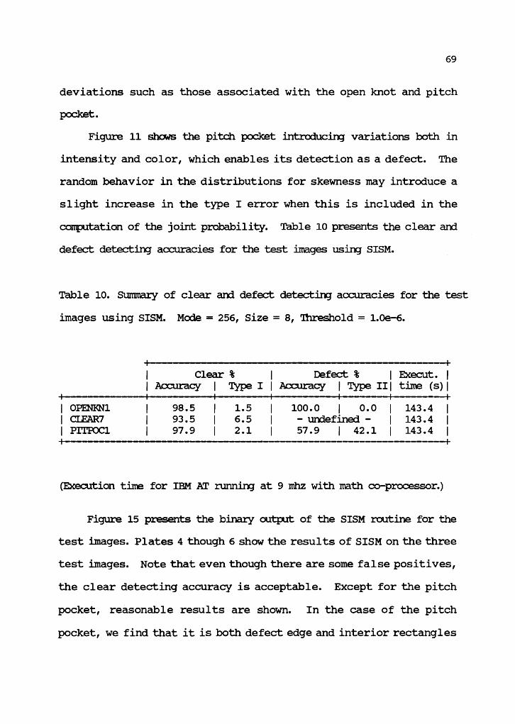
Clear %I
Defect %IExecut. I
Accuracy I 'type I I Accuracy I Type III tine (s) I
---+I 1.5 I 100.0 I 0.0 I 143.4 I
I 6.5I
- undefined - I 143.4 I
I 2.1I
57.9 I 42.1 I 143.4 I
(Execution time for IBM AT running at 9 nbz with math co-processor.)
Figure 15 presents the binary output of the SISM routine for the
test images. Plates 4 though 6 show the results of SISM on the three
test images. Note that even though there are some false positives,
the clear detecting accuracy is acceptable. Except for the pitch
pocket, reasonable results are shown. In the case of the pitch
pocket, we find that it is both defect edge and interior rectangles
69
deviations such as those associated with the open knot and pitch
pocket.
Figure 11 shags the pitch pocket introducing variations both in
intensity and color, which enables its detection as a defect. The
random behavior in the distributions for skewness may introduce a
slight increase in the type I error when this is included in the
computation of the joint probability. Table 10 presents the clear and
defect detecting accuracies for the test images using SISM.
Table 10. Summary of clear and defect detecting accuracies for the test
images using SISM. Mode = 256, Size = 8, Threshold = 1.0e-6.
OPENKN1 98.5CLEAR7 93.5PITPOC1 97.9

70
which contribute to the high type II error. Such location errors
could be recovered by a post-processing step.
7.5 =MED ANALYSIS OF MISM ON THREE TYPIML IMAGES
Where SISM relies on Treasures of central tendency, MISM extracts
texture Treasures. Texture analysis applied to images of wood surfaces
could be very effective as these surfaces are rich in texture. The
anisotropic nature of wood is well-known. The proposed methodology
as defined under "methodology for application in this thesis" uses
morphological operations which are sensitive to both feature size and
alignment. Such an arrangement should theoretically be able to
capture the kind of texture which is apparent in wood surfaces.
The results of MISM on the test images are presented by showing
the response at 0, 45, 90 and 135 degrees orientation, relative to the
horizontal. By presenting only advanced (eighth iteration) states of
the process, it is easier to explain the behavior of the largerdefects, such as those present on the test images. However, responses
to features such as wood grain are included in the full analysis.
Figure 16 presents the results of a progression of morphological
operations using a structuring element which consists of a line
segment of varying length and orientation on OPENI<N1. The test images
were all oriented such that grain direction was horizontal (0degrees). Consequently, along-the-grain operators show the smallest
effect.

71
The early iterations (i.e., using smaller line segments) in a
MISM process produce similar results to computing the mean value over
a rectangle. This is comparable to how SISM computes its mean
measure. Higher iterations (i.e., longer line segments) have the
ability to reject background features and enhance the features of
defects. It is this feature which may contribute important
structural or texture information.
Figure 17 presents the results of MISM applied to a clear sample
with heavy earlywood/latewood pattern. This also shows minimum
response with along-the-grain orientation. The other orientations
show similar responses.
Figure 18 presents the results of MISM applied to a sample
containing a pitch pocket. Note that several of the rectangles
spanning the pitch pocket are lost. This is often the case where a
rectangle boundary and an artifact boundary align. When the following
rectangle falls completely within the defect, with very uniform
characteristics, neither defect boundary nor interior will be sensed.
Table 11 presents the clear and defect detecting accuracies forMISM on the test images. Figure 19 presents the binary output images
of MISM applied to the test images. Note that MISM uses a lower
resolution rectangle (16x16 pixels) and thus the results in smaller
binary images canparea to SISM or CISM. This larger rectangle size is
necessary because MISM requires the presence of structure to work
efficiently. Wood contains several types of structural properties,
however it is mainly the earlywood/latewood structure that is

OPENKN1I CLEAR7I PITPOC1
89.9 1 10.1 1
53.6 1 46.4 1
80.8 1 19.2 1
66.7 1 33.3 1
- undefined - 1
66.7 1 33.3 1
418.5 1
418.5 1
418.5 1
(Execution time for IBM AT running at 9 rnhz with math co-processor.)
Plates 7 through 9 shag the results of MISM on three test images.
These unexpected disappointing results of MISM include a relativelyhigh type II error as well as marginal clear detecting accuracy.Several factors may contribute to these results. One of the reasons
is that only intensity information was considered in this thesis. The
high type II error for the pitch pocket may well be attributed tothis. Another serious problem, which I mentioned before, is theeffect of artifact boundaries. Re-analysis of an image with small
translation of bcurrlaries may produce significantly different results.It might be possible to include sane form of edge dithering. However,
with our present hardware, the computational demand makes that
impractical. With special pipelined architecture where processing
could be performed in a frame time (1/30 sec), this may indeed be
72
important to MUM On the smaller rectangle sizes, i.e. 8 x 8, therejust is not sufficient evidence of this type of structure.
Table 11. Summary of clear and defect detection accuracies for thetest images using MISM. Mode = 256, Size = 16, Threshold = 1.0e-12.
Clear %I Defect %
I Doacut. I
I Accuracy I Type I I Accuracy I Type tilne (s) I

possible.
7.6 DETAILED ANALYSIS OF CISM ON THREE TYPICAL IMAGES
Where SISM computed a series of measures of central tendency,
CISM computes k means in defining its clusters. As described in
"methodology for application in this thesis", the first step is to
determine a set of rectangles which conforms to certain criteria of
homogeneity. The value used as a criterion for homogeneity in this
case is the sum of variances of the measures which is called the
measure of dispersion. The computed values of dispersion over the
three test images are presented in Figure 20. From this graph a value
of 2.0 for a dispersion threshold has been selected and used in
subsequent analysis. Note that the three images have similar
dispersion graphs and further that a definite step exists. This
indicates that the measure of homogeneity does not relate to a
quantity that changes gradually, hit rather abruptly.
The next step then involves the application of the isodata
algorithm. This is an iterative procedure for determining the k,
means. Once known, these k mean values are used to flag rectangles
that are "too far" away from them. A distance measure, or so called
heuristic function, uses both color and intensity channels as well as
the extracted measures of how compact or spread out the cluster
appears to be in order to compute a rectangle's distance from the
cluster. A series of figures presenting the clustering in the test
73

74
images are presented in Figure 21.
Figure 21 presents the clustering of OPENKN1, CLEAR7, and
PITPOC1. Note that for these images there generally exists only a
main cluster. It is expected that when other types of defects, for
example stains and fungal discoloration, are analyzed, more clusters
would be apparent. It may then be necessary to revise the heuristic
function to include the notion of multiple clusters. The form of the
heuristic function as used in this thesis uses the idea of simple
single clustering. Note that for OPENKN1, values associated with the
open knot are clearly outside the main clustering. Further, the
effect is both in intensity and color channels. This is also noticed
in PITPOC1, where the values associated with the pitch pocket are
clearly distinct from the main cluster. Such a distinct separation
distance is a desirable feature for detecting defects.
An interesting observation is the orthogonality of intensity and
color (clusters near circular, shcwing little, or no interdependence
of the two channels). This shows how successful the transformation
suggested by Ohta (1980) could be carried through.
Table 12 presents the output of the isodata algorithm on the test
images. This table shows that for the chosen dispersion value,
roughly 50% of the rectangles were considered hanogeneous (this set is
called the core candidate vectors). This observation may be
surprising to a human observer who would consider some of the samples
as "normal". This confirms the complex nature of wood with which
autanatic machinery has to deal with. This observation is especially

75
applicable to CLEAR7 which had the least number of homogeneous
rectangles. This variation is introduced by the dominant
earlywood/latewood patterns. Note further that a unique set of k
means (core vectors) have been derived for each sample. This
indicates sane between-santple variation. A further point of interest
is the occurrence of mans with law counts associated with them. It
is questionable whether these minor core-vectors should be considered
part of the main clusters or not. This is one topic which will be
explored under "Considerations for tuning the algorithms".
Table 13 presents the results of CISM using the simple heuristic
as described above. Figure 22 presents the binary output images of
CISM on the test images. Plates 10 through 12 show the results of
CISM on the three test images. These images show that CISM has
worthwhile properties.
Note the law type II error produced by CTSM on these particular
samples. It is sham in section 7.7 "analysis of the ISM algorithms
on a larger test set", that CISM produces nuch higher type II errors,
particularly with pitch pockets.
The results of the three pre-processing algorithms are presented
in Table 14 to sumarize this detailed analysis of three test images.
Note that for sake of brevity, only the percentage clear and defect
accuracy are presented. It is trivial to derive the type I and type
II error percentage from these. These results should not be used for
comparative purposes, but rather should serve as a crude guide as to
what such algorithms are capable of.

Table 12. Core vectors for the three test images.
Mode = 256, Size = 8
Dispersion threshold = 2.0
Number of clusters = 5
Total number of rectangles = 800
I number core I Core vectors
I Sample 1 candidates 1
OPENEN1I
415I
76
Intensity Color count I
15.8956 19.3182 2219.2969 19.2253 3618.2654 19.1844 8716.7347 19.2023 13617.3701 19.1447 134
14.9308 19.4621 2119.1374 18.9241 8616.1462 19.4274 6517.2371 19.1273 6918.3301 18.9216 97
14.5521 19.7188 6
19.8416 18.4234 5116.7535 18.8429 7117.9859 18.5093 14918.8553 18.4411 104
CLEAR7 338
PITFOC1 381

Clear %I
Defect %1 Execut. 1
Accuracy 1 Type II
Accuracy 1 Type III time (s)1+-1 OPENKM1 I 97.6 1 2.4 I 60.0 1 4.0 I 140.6 I
1 CLEAR7 I 91.9 1 8.1I - undefined - 1 119.5 1
I PrmociI 99.2 1 0.8
I94.7 1 5.0 1 145.9 I
mean I 135.3 I
(Execution time for IBM AT runnirxj a 9 mhz with math co-processor).
Table 14. Summary of results of SISM, MISM, and CISM on OPENKN1,
CLEAR7, and PTTPOC1.
77
Table 13. Summary of clear and defect detection accuracies for the
test images using CISM. Mode = 256, Size = 8.
% Clear Accuracy 11 % Defect AccuracYSISMI MISMI CISM II SISM 1 MISM 1 CISM
If97.6 11 100 166.7 160.01
91.9 11 - undefined -99.2 11 57.9 1 66.7 1 94.7
135.31
OPENKN1 98.5 89.9CLEAR7 93.5 53.6PITPOC1 97.9 80.8
Exec. tiiiI 143.41 418.51

7.7 ANALYSIS OF THE ISM AILORITHMS ON A LARGER TEST SRI'
The previous section gave an in-depth look at how the different
ISM algorithms functioned. A preliminary comparison of their merits
was presented in Table 14. However, there is a need for morestatistical significance. For this purpose, a more comprehensive test
was devised including a larger sample set.
The algorithms were subsequently applied to a set of samples
representing the three common defect types, i.e., open knots, closed
knots, and pitch pockets. Five replications of each type of defect
are included. This set of results also serves as the basis forcomparing the improvements gained by tuning the algorithm. Table 15
presents the results of the algorithm applied to this sample set
When interpreting these results, the reader is reminded that it
is of primary importance to consider the defect detecting accuracy.
However, when this corresponds to an exceptionally laa clear detecting
accuracy, the algorithm is most probably not working too well.
(Consider a case where all rectangles are marked as defective, then
the defect detecting accuracy will be 100% and the clear detecting
accuracy will be 0% - clearly a poorly performing algorithm).
Using this crude rating criterion, MISM (91.56% +/- 3.41) is
rated marginally highest followed by SISM (87.8% +/- 3.69) and CISM
(78.3% +/- 4.58). Considering the three types of defect, MISM
produced consistent defect detecting accuracy, but had the lowest
clear detecting accuracy (79.99% vs. 93.11 and 95.47%).
78

SampleI
SISKI
MISK1
CISMdesig.
I%clear %defect
I%clear %defect I %clear %defect
OPENEN1 I 98.5 100.0I
OPENEN2 I 92.0 100.0I
OPENEN3 92.6 90.5 I
OPENKN4 91.8 100.0I
OPENKN5 89.5 100.0I
mean I 92.88 98.10I
+- ______+Istd.dev.
I1.83 2.06 1
i
(b) CLOSED IZICTS
SampleI SISK
I I CISKdesig. I
CLEN1 I
CLEN2 I
CLEMICLKN4 I
CIENS I
mean I
I std.dev.1
79
Table 15. Comparative results of SISM, MISM, and CISM applied to
three common defects of Douglas-fir veneer surfaces. (a) Open knots,
(b) Closed knots, (c) Pitch pockets. (d) overall (all samples
pooled).
For all these: Mode = 256, Size = 8 (16 for MISM), Threshold = 1.0e-6
(Threshold = 1.0e-12 for MISM).
(a) OPEN KNOTS
%clear %defect I %clear %defect 1 %clear %defect
88.5 100.0 46.8 75.0 91.4 100.094.6 78.9 70.4 100.0 93.3 84.294.3 75.0 66.1 100.0 96.1 91.794.9 100.0 89.2 83.3 93.8 100.097.2 100.0 89.4 100.0 92.9 85.7
93.9 90.78 72.38 91.66 93.5 92.32-+
1.80 3.56 4.22 3.43 1.31 2.75-+
89.9 66.7 97.6 60.081.0 100.0 98.6 95.889.2 100.0 98.6 95.292.6 100.0 90.9 57.169.7 100.0 79.7 100.0
-+84.48 93.34 93.08 81.62
---+ -+3.05 3.86 2.85 4.60
--+- --+

Table 15. (contd)
(c) PITCH poczErs
desig. I %clear %defectI%clear %defect
I
Sample I SISKI MISK I CISM
PPOCI 97.9 57.9PPOC2 82.8 78.7PPOC3 95.7 75.0PPOC4 93.0 86.0PP005 93.3 75.0
mean 92.54 74.52I
std.dev.I 2.0 3.69I
+11MAINOMIMIMIMNINIIMMNNMINIMOMPINMMNIMIIONIMAIMININ.14.1401 1=IMMMINIMM+
(d) OVERALL.
man 1 93.11 87.8 1 79.99 91.56 1 95.47 78.31 I
IINFINOMI.11M+
In the next section I will shaw that these results of MISM cannot
be improved by simple tuning. Both SISM and CISM can be tuned to
produce superior results to Nam'. Thus, unless the clear detection
accuracy of PDLSM cculd be improved significantly (by at least 10%),
the other algorithms are favoced.
80
%clear %defect
99.2 94.7100.0 62.3100.0 54.2100.0 48.8100.0 45.0
99.84 61.0
2.34 4.58
92.7 73.376.3 94.790.8 87.570.8 92.984.9 100.0
83.1 89.68
3.62 3.41
I std. dev. 1 2.0 3.69 1 3.62 3.41 1 2.34 4.58 1
I
I

8. CONSIDERATIONS FOR TUNING THE ALGORITHMS
The purpose of this section was to improve the performance of
the ISM algorithms, if possible. The results of the three algorithms
were analyzed for reasons why it failed under certain conditions.
Some useful clues were found which made it possible to make some
improvement.
8.1 TUNING SISM
Several factors may influence the outcome of SISM. However, it is
especially sensitive to the make-up of the decision-making rule.
Let's review sane of the feature selection methodology as described in
the literature review. The first step towards producing a set of near-
optimal parameters is to pick out those which best reflect the
physical constraints associated with images of wood surfaces. It is
useful as a further step to remove redundant ones. When these
distinctions are not clear, or when there are too many, such a
selection process may be carried out using discriminant analysis.
Kruger et al. (1974) describes such a methodology where a pair of
features are tested for "divergence". By ranking pairs by their
divergence measures, an optimal set can be selected.
Such a detailed analysis was not attempted in the case of SISM.
The exploratory statistical analysis presented in the section
"detailed analysis of SISM on three typical images", provided some
81

82
clear guidelines. Inspection of the graphs of the statistical
measures (intensity/color means, variance, skewness and kurtosis)
showed that for the veneer surfaces, only mean, variance, and kurtosis
contain useful information. Of these, variance and kurtosis show
similar responses, thus one may be regarded as being redundant. This
reduces the feature set to four, i.e., means of intensity and color,
and variance of intensity and color.
Of further importance is the goodness of estimation of the
probability density functions. The graphs of the variance values used
in the first approach showed that sane improvements were possible. As
an exarnple, improved estimation of these variances are presented in
Figures 23 through 25. These figures present a "well-behaved" image
and two "ill-behaved" ones. Compare the extent of variation
corresponding to the defect in each case. Further note that for the
well-behaved case, the signal of the defect is obvious (note the
arrows) while in the ill-behaved case, several of the measures
contribute little or no information about the presence of the defect.
Figure 24 presents an image where information is present only in
the intensity channel (mean and variance). Figure 25 presents an
image where only the mean of the color channel carries useful
information. This is an important discovery: that information may be
present only in the intensity, or only in the color channel, or
simultaneously in both intensity and color channels. Knowledge of
this fact is essential when designing a reasonable decision rule.
However, for this study, the four parameters are weighted equally in

results.
I Sample I Clear % I Defect % I
NO. 1 Before After I Before AfterI
I 100.0 100.0 I
I undefinedI
I 57.9 93.0 I
83
the rule. This is achieved by a normalization procedure which assures
that the most frequently occurring combination of features' joint
probability canes out as unity.
Plates 14 through 16 present the operation of the tuned SISM
algorithm on the test images OPENKN1, CLEAR7, and PITPOC1. Note that
except for CLEAR7, both defect and clear detection accuracies have
improved. Table 16 presents the results of the tuned SISM algorithm
on the test images.
Table 16. Results of tuned SISM on OPENKN1, CLEAR7, and PITPOC1.
Mode = 256, Size = 8, Threshold = 10.0e-3.
To ensure reliable reduction of the type II errors, a higher
threshold was selected for the more carprehensive test set. Table 17
presents the results of the tuned algorithm on this sample set Note
that the defect detection accuracy has been improved by 11.94% at a
cost of a clear detection accuracy of 3.84%. Another significant
improvement is shown in the reduced amount of variation in the test
OPENKN1 I 98.5 97.3
I CLEAR7 I 93.5 96.3
I PITFOC1 I 97.9 97.8

CLKN1CLKN2CLKN3CLKN4CLKN5
PPOC1I
97.9 89.7PPO22 82.8 84.3PPOC3 I 95.7 93.8PPOC4
I93.0 85.5
PP005I 93.3 89.2
88.5 86.994.6 88.594.3 89.194.9 90.197.2 89.4
I std.dev. 1 2.0 1.53 I
100.0 100.078.9 100.075.0 100.0
100.0 100.0100.0 100.0
-+57.9 97.778.7 98.475.0 100.086.0 100.075.0 100.0
means I 93.11 89.27 I 87.8 99.74
3.69 0.84-+
84
Table 17. Results of tuned SISM applied to three common defects of
Douglas-fir veneer surfaces. Mode = 256, Size = 8,
Threshold = 50.0e-3.
+ -+I Sample Clear% Defect%
Ino. Before After Before After
+ -+ -+ -±OPENEN1 98.5 91.7 100.0 100.0OPENKN2 92.0 89.7 100.0 100.0CTENKN3 92.6 90.2 90.5 100.0CTENKN4 91.8 91.0 100.0 100.0CTENKM5 89.5 90.0 100.0 100.0
A very worthwhile improvement would be to include dynamic
threshold estimation. Figure 26(a) shads the joint probability for a
well-behaved image. Well-behaved in this sense means that both the
intensity and color channels provide supportive information of the
defect. Note that the curve appears near-horizontal with several
plateaus. These plateaus are possible thresholding points. Contrast

85
this image's behavior with Figure 26(b). In this ill-behaved image,
there is no useful information in the color channel. Further, the
size of the defect is large (approximately 20% of the total image).
These two confounding factors produce a resulting joint probability
function with a steep slope. The plateaus on this curve are also
less-pronounced; however, by choosing the most-pronounced one (i.e.,
at 65.0e-3), 100% defect detection is attainable.
Whether such a scheme belongs at the low level pre-processing
stage or at the main processing stage, depends on representation and
searc4 considerations. For this study, fixed threshold (global)
values are used.
8.2 TUNING MISM
Attempts to improve the results of MISM were not successful. As
a first step, the number of intervals for the estimation of the
probability density function was increased. This made no significant
improvement, indicating that the original estimation was adequate. As
was stated in the section on "analysis of the ISM algorithms on a
larger test set", MISM would became an attractive alternative if the
clear detecting accuracy could be improved by at least 10%. Such a
dramatic increase is not possible without the investigation of the
importance of an extended color feature set. This was not pursued
further as it was unlikely that a better solution than that offered by
SISM would be forthcoming.

8.3 TUNING CISM
In the section "detailed analysis of CISM on three typical
images", the components of the decision heuristic were reviewed. It
was also indicated that CISM shows very promising results and has the
potential of relating well to some physical constraints (unknown at
the moment) associated with perception of defects on veneer surfaces.
Cluster analysis deals with how parameters are grouped.
Psychologists, especially those of the "Gestalt school", have paid
considerable attention to the psychology of visual association and the
grouping preferences that humans have. Cluster analysis depends
largely on how well the cluster model is interpreted, i.e., whether
the main parameters have been identified or hay well the cluster shape
is understood, or whether single or multiple clusters should be
expected, etc.
The success of locating defects with CISM depends largely on the
heuristic used in the decision rule and had well this relates to the
interpretation of the cluster model. As a first approach, the
heuristic was chosen such that the distance of any rectangle to its
nearest core vector, did not exceed half the farthest distance
between any two core vectors. This heuristic is inherently dependent
on how well the core vectors represent clustering.
The isodata algorithm which determines these core vectors is
basically a k-mean estimator. For this study, k equals five (an
arbitrary choice). Table 12 showed that in some cases the number of
86

87
points associated with certain core vectors are minimal. This
indicates that perhaps those might be of lesser significance, or more
likely to be associated with sane minor flaw.
As a first step towards tuning CISM, these core vectors were not
considered during the mark phase. Table 18 shows the results of the
tuned CISM algorithm using this method.
Note that roughly half the samples did not contain any minor core
vectors. For these cases, results are unchanged. Overall, a 9.11%
increase in defect detecting accuracy was realized at a cost of a
7.74% reduction of clear detecting accuracy. Further note that the
variation in defect detecting accuracy has also been reduced. However,
the variation of clear detecting has increased.
Some further improvement to the decision heuristic might result
by including sane measures of spatial relationships. Note that the
decision rule only uses the relationship between the intensity and
color channels. Frequently, in the case of isolated pixels that are
incorrectly marked, a simple neighborhood test would have resulted in
the correct action taken. This was not attempted in this thesis
because such connectivity may be more involved than is indicated is
better left to the later processing algorithms.
Execution time for CISM is dependent on the image being analyzed.
The suggested tuning procedure for CISM will have little or no effect
on the execution time as generally only one or at most two core
vectors would be excluded.

OPENKN1OPENKN2°MEMOOPENKN4OPENKN5
CLKN1CLIZT2CIAKN3
CLKN4CLKN5
PPOC1PPOC2PPOC3PPOC4PP005
means
97.6 97.698.6 84.198.6 84.590.9 90.979.7 79.7
91.4 91.493.3 93.396.1 85.493.8 84.692.9 92.9
99.2 89.3100.0 100.0100.0 96.4100.0 49.9100.0 96.0
1 95.47 87.73
60.0 60.0 *95.8 100.095.2 95.257.1 57.1 *100.0 100.0 *
100.0 100.0 *84.2 84.2 *91.7 100.0100.0 100.085.7 85.7 *
94.7 97.762.3 62.3 *54.2 100.048.8 79.145.0 90.0
___+
1 78.31 87.42
I std. dev. 1 2.34
( * - no minor core vectors present, results unchanged )
To conclude this section on tuning the algorithms, a summary of
the best results using the tuned versions of the algorithms are
presented in Table 19.
0//011.
3.46 1 4.58 3.98
88
Table 18. Results of tuned CISM applied to three common defects of
Douglas-fir veneer surfaces. Mode = 256, Size = 8.
Sample Clear % Defect %No. Before After Before After

Table 19. Surnmarized results
versions of the ISM algorithms on
fir veneer. Mode = 256, size = 8
1.0e-6, Tuned threshold = 50.0e-3,
I SampleI No.
I Open knotI
'Closed knotI
IPitch pocket I
means
I std.dev.
I Sample I
I No.A
I CPen knot I
IClosed knot I
I Pitch pocket I
(a) Uhtuned results of the ISM algorithms.
SLSM
90.54 100.088.8 100.088.5 99.22
of the (a) untuned and (b) tuned
the three cara-non defects of Douglas-
(16 for MISM), Untuned threshold =
Threshold for MISM = 1.0e-12.
MISM
84.4872.3883.1
(b) Tuned results of ISM algorithms.
93.3491.6689.68
89
-+CISM
%defect I
81.62I
92.32 I
61.00 I
-1-78.31 I
4.58 I
SISMI MISM
ICISM
%clear %defectI%clear %defect
I%clear %defect
I
--+87.36 82.46 I
89.52 93.98 I
86.32 85.82 I
%clear %defect %clear %defect %clear
92.88 98.10 84.48 93.34 93.0893.90 90.78 72.38 91.66 93.5092.54 74.52 83.1 89.68 99.84
93.11 87.80 79.99 91.56 95.47
2.0 3.69 3.62 3.41 2.34
meansI 89.28 99.74 I 79.99 91.56
I87.73 87.42 I
I std.dev. I 1.53 0.84 I 3.62 3.41 3.46 3.98 I

9. SUMMARY AND DISCUSSION
In this summary I will emphasize those topics in this thesis
which influenced the direction taken and subsequent outcome. Several
important conclusions will also be presented.
The purpose of this thesis, in general terms, was to investigate
potential methodology and develop algorithms, which, when applied to
images of Douglas-fir veneer, would reduce image complexity. This is
considered an essential step towards the achievement of an automated
veneer plugging system. As such, these algorithms should be
computationally efficient, and yet be highly reliable in focusing on
potential defects.
The literature survey for this thesis was extensive. This is an
indication of the diversity of the thesis topic, and is also in part
due to the multidisciplinary nature of the field.
Several papers confirmed the monotone color of wood. Its
dominant wavelength is rcughly 580 ran, and its color variability is in
brightness and purity. The C.I.E. tri-chromatic system forms the
basis of measureraent, but when considering the limited range of
variation in the color of wood, this system is inadequate. Using
Ohta's (1983) work on the derivation of an alternative color model,
this thesis showed that the color of Douglas-fir veneer surfaces is
consistently two-dimensional. This fundamental concept is applied in
all three algorithms to extract features.
The papers by Conners et al. (1983, 1984a,1984b,1985) suggested a
90

91
first-order statistical analysis in a hierarchically organized system.
This idea provided the basis for the SISM algorithm. It furtherpresented useful ideas, as well as served as a rough benchmark as to
what could be achieved. However, no valid comparison between the
results of this thesis and those from Conners et al.(1983,1984a,1984b,1985) can be made unless SISM can be tested on the
same sample set that they used. The difference in species as well as
the type of surfaces analyzed in this thesis are significantlydifferent.
Werrnan and Peleg (1985) suggested a novel texture analysis
technique based on mathematical morphology. This idea formed thebasis for the MUM algorithm. Not only is texture an importantfeature of wood, but morphology offers some possibilities forimplementation on specialized hardware. It is also worthwhile to note
the relative merits of this method as this hardware is presentlymaking its way into equipment for application in the forest productsindustry.
Some very useful, though originally obscure, methodologies were
obtained fram Fukada (um) on spatial clustering. This paper formed
the basis for the CISM algorithm
Marr (1980) provided confidence that, in principle, ISM is a
valid and important step. As such, ISM may be considered a step
toward the derivation of the primal sketch and perhaps in a broader
sense, a first-order analyzer.
The formal definition of SISM, MISM, and CISM provided three ways

92
of locating defects by observing deviations fram: measures of central
tendency of first-order probabilistic differences, measures of central
tendency of morphological texture measures, and clustering tendency.
Even with this limited theoretical definition, a nearly unlimited
number of controlled experiments are possible. This thesis provides a
first attempt at what ISM may offer. As indicated, there are other
possibilities to explore.
The three ISM algorithms have some common principles. Of
fundamental importance is the derivation of a set of working measures,
then the determination of their behavior over an image, followed by a
postiori determination of those elements which deviate from "normal".
This approach deviates frau a conventional Bayesian classifier in that
no training set is involved. During the course of the experiments,
such an approach using a railti-class classifier and a training set was
implemented and tested. It was found that there was so much
variability present in the images of the veneer surfaces that
estimation of the number of classes and their features was beyond the
scope of this thesis. A crude estimation produced unacceptable
results. As a result of this complexity, a simpler approach was
followed using the joint probability function.
A follow-up on the results of those experiments that showed poor
performance of the ISM algorithms, in particular during the testing of
SISM, indicated that the type of defect present on Douglas-fir veneer
surfaces manifests in three possible ways: as an intensity effect, as
a color effect, or as both intensity and color. This result is of
93
principal importance, as knowledge of this fact needs to be included
in the decision-making rule of any successful defect-detecting
algorithm. It further stresses the importance of color in addition to
black-and-white imagery. This is important as presently only black-
and-white image processing systems are employed in forest products
applications. Very little is actually known about the importance of
color for these applications.
The conclusive result of the experiments indicated that SISM
consistently produced the best defect detection accuracy (99.74%) as
well as the best clear detection accuracy (89.28%). This result
translates to a significant achievement. For example, if defects
occupy 10% or less of the total area analyzed (a conservative
estimate), then this means that the image data can reliably be reduced
by 80.4% (89.28% x (100-10%)) while ensuring a type II error of 0.26%
(100-99.74%). The importance of this result is twofold: The reduced
image data contains only essential information on which to perform
defect detection, thus redwing the carplexity of the post-processing
algorithms. This factor may make the difference between whether or
not real-time operation is possible.
This thesis did not consider ISM as a means to an end, but rather
a step in a complex chain of processes. Besides its intended function
of focusing attention on potential defects, its intermediate results,
when incorporated in a proper representation may provide useful clues
to higher-order processing algorithms.

10. FIGURES
10.1 PREFACE TO THE FIGURES
Sane of the figures need further clarification. Figures 3 through
14, 16 through 18, and 23 through 25 have similar layout. These
graphs are essentially two-dimensional representations of three-
dimensimal quantities.
On the horizontal axis, each unit represent a single row of
adjacent rectangles fram the original image, several pieced together
in linear fashion. The horizontal axis thus represent the image as
scanned from the bottom left corner to the top righthand corner, mfr./
after row. Thus even when the trends show regular repetitive
waveforms, each wave is actually only representing one scanned row of
the image.
Where possible, the position within a raw where a defect occurs is
sham with arrows. The corresponding categories for these defects are
then sham with arrows in the smaller win -like histograms.
For a comprehensive discussion of the graphs please see section 7.2
"a note on the interpretation of the graphical material".
94

0.4
>0.3
3 0.2
2R 0.1
Ec- 0 400
-0.1
Figure la: Tristimulus values of C.I.E. spectralprimaries required to match unit energythroughout the visible spectrum.(From Pratt (1978))
1 I
0
(X)&.G (X)
R (X. )
600 700WAVELENGTH, n m
95
S.
520
S31
i
SN
4
W
610
1411
/03
410
40
02 03 04 as 05 01 05X
Figure lb: C.I.E. Standard Observers'Chromaticity Chart. (From Beck'sbook Color Perception.)

1 20' x IS" 1
+ +1 10" x 7.5" 1
1 image size1 5" x 3.75"
1 512 x 512 256 x 256 1
1 128 x 128 11 64 x 64 1
+ +-+ + + +1 32 x 32 .
4 16 x 16 1
1 + +-+ + + +/->-1 rect. size 1 :rect. size 1-<-\
4 .4. , 16 x 16 1
4 .. 8 x 8 .
. .
+ + + +
+ +. .. . testing procedure\ < 1 using 1 > /
(adjust rec- 1 worst case samples (adjust rectanoletangle size or + + size)
image size )
Figure 2: A method for evaluating minimum image resolution.
96

a)
2625 -2 4. -23 -22 -21 -20 -1 9 -1 8 -1 7 -
22
21
20-
19 _04144SA"WM")0410441114A14444"
1 8 -
1 7 -
1 6 -
1 5 -
b) 14- 01 2 3 4 5 6 7 8 9 1011121314ROW SCANNED
150
co
so
"Ilett*AA11(400.10.4/4'MEAN
A OPINKMINCO
WO-
4c°
E
2C0
MD-
=OR
Figure 3: Mean values for (a) intensity and(b) color for OPENKN1.
t.2 Ila 184 17a t* 202 22.4 210 10
.avarrr
97
A22.5
g
0 1 2 3 5 6 7 8 9 1011121314L1ROW SCANNED

a
1 0
9 -
7 -
1 - NII°4444#8$1141111
3 -
2
MM1)10\4041A110\iiii0\iti
0 1 ' 3 4- 5 6 7 8 9 1011121314-15161718192021222324-2!ROW SCANNED
VARIANCE
VARIANCE
Figure 4: Variance for (a) intensity and(b) color for OPENKN1.
0 1 2 3 4 5 6 7 8 9 10111213141516171819202122232425ROW SCANNED
98

b)
1 0
9
8 -7
42
-0 -lowistvvvonoiHri
1 -
10
9
7
65
*
2
1 -
3 4 5 6 7 8 9 1011121314151617181920212223242!ROW SCANNED
4
a
0 '-`5"."`-0 0 0 A
SKEWNESS0.001.10.
1102141TI
Figure 5: Skewness for (a) intensity andm color for OPENKN1.
SK EWN ES S
0 1 2 3 4 5 6 7 8 9 10111213141516171819202122232425ROW SCANNED
99
a) 4 -r01

30282624
201816
141210
8
a) 0
30282624222
1
1
1
1
1
86
42
0
8
6
-1--
-1
i10,01`( g)
8 9 1011 1 2 131 415 16 7 1819 20 21 22 23 24 25ROW SCANNED
ki0p,
KURTOSIS
WIEPOrtY
KURTOSIS
CO..
F0 _--S4.4.4.4.44,-(r"wom.c...f40.-ArvvvVIA,"VvioVrivA>k4eAm0440 LAAAL44.044,4:11114m14.4""krivr9.1..'sm,-,,v-ri.
0 1 2 3 4 5 6 7 8 9101112131415161718192021222324-25ROW SCANNED
Figure 6: Kurtosis for (a) intensity andm color for OPENKN1.
100
601 2 3 4- 5

22
21
20
19
18
17
16
15
b) 14
0 1 2 3 4 5 6 7 3 9 1011121314ROW SCANNED
0 1 2 3 4 5 6 7 8 9 1011121314
Figure 7: Mean values for (a) intensity and(b) color for CLEAR7.
MEANCLE.7
174 170 102 .0.4 If if 202 200 21
ROW SCANNED COLOR
101
142 1 4 'fa 17. t'S 21;2 2;
41/T,Gt7f
26
2423
21
20191817161514131211
a) 10

a
10
9 -
7 -
6 -
5 -
-
3 -
2 -
o -0 1 2 3 4 5 6 7 8 9101112131415161718192021222324-25
ROW SCANNED
Figure 8: Variance for (a) intensity and(b) color for CLEAR7.
VARIANCE
7/z
02,11/
2 23 3
COLOR
0 1 2 3 4 5 6 7 8 9 101112131415161713192021222324-25ROW SCANNED
VARIANCE
102

M
1
a) 4.0 1 .., 3 4 5 6 7 8 9 10111213141516171819202122232425
ROW SCANNED
0 1 2 3 4 5 6 7 8 9 10111213141516171819202122232425ROW SCANNED
Figure 9: Skewness for (a) intensity and(b) color for CLEAR?.
103
1 0SKEWNESS
9
8
7
6-5-43
0 I " I 1 ,.5,1 rr
2m.
nA vu
-0 5 0 0 I
5011M5trY

3028262422201816141210
8
6
2
0
3028262422201816141210a6
42
NiA/MtvvVr4r0,1
0 1 2 3 4 5
ROW SCANNED
KURTOSISCl2.4147
400
3c°a
203
KURTOSIS
141516171819202122232425
C01241
Figure 10: Kurtosis for (a) intensity and(b) color for CLEAR7.
1"0"A"AVV"011itAr4PISIAvti46NAVNP11444.41,.4911067 8 9 10111213141516171819202122232425
ROW SCANNED
104
1 4 3

a
2625 -
-232221 -20 -19 -18 -17 -1,11
16 -
20 -
19 -
18 -
MEANmoot
410/21111rf
MEAN
V
V1171 .
.24 104 302 2041
V
1011 1213141516171819 20 2122 23 2425ROW SCANNED
VV
1011 12131415161718 19 20 2122 23 2425ROW SCANNED
Figure 11: Mean values for (a) intensity and(b) color for PITPOC1.
105
14.2 1144 1114 171 202 21 221I Urn
22
21

VARIANCE111/PCC 1
0 1 2 3 4 5 6 7 8 9 10111213141516171819202122232425ROW SCANNED
Figure 12: Variance for (a) intensity and(b) color for PITPOC1.
106
1
<
8
0VARIANCE
01.CC
9 -
-7 -
6-5-
-
3 -
2 -
1 -
100
VOA
fr
vv
1 Lb
OUP3.0
in111117 8 9 10111213141516171819202122232425ROW SCANNED
0 1 2 3 4 5 6

b)
1 0
9
8
7
6
5
-3
2
kwArotrsvoteiroitruire.tiNvsoivfwivriywwft.001,fro_
3
a) 40 1 2 3 4 5 6 7 8 910111213141516171819209122232425
ROW SCANNED
SKEWNESSomm
0 1 2 3 4 5 6 7 8 9 10111213141516171819202122232425ROW SCANNED
Figure 13: Skewness for (a) intensity andcolor for PITPOC1.
107
-0 01 I
11110111

a)
130
241
2ia311
21 ce.18 1°'
16.0.14-r:12- 0
108
00 1 2 3 4 5 6 7 8 9 10111213 41516171819202122232425
ROW SCANNED
302826 .
=24 m
20 ode
18 1016 -
1210
86
-2
KURTOSISPM= t
. 1 AI IA a a. aa 401
MM
108
0 1 2 3 .4 5 6 7 8 9 10111213141516171819202122232425ROW SCANNED
Figure 14: Kurtosis for (a) intensity and(b) color for PITPOC1.
30 2.3
28 MI32I
26
KURTOSIS11111M1

MMMMM a
MMMMMMMMMM
IMMO MIME MMMMMMMMMMMMMM
MUMMOMMEMONOMOMMOMMOMMOMMMIMUMMIOMEMMUSOIRMIOMMUMOMOIMIll
SO. MOM M MMMMM MO MMMMMM Mann
II II II II MI IN II II IS MI ill II II IN MI MI MI in ID el II El MI II
menunwnwinnnwin. MMMMM nomS
II II II II 61 II II II II II II IR II II II II 111 II MI II IIIN II II II II II II IN II IS II 61 II II 61 II II II II II II II II OS II
maul MMMMM
ME MMMMMMMMMMMMMMM MUMOMIIMMIN
inninnonnonnwommonnnannsninnnom MMMMM nomninnnnunninsinnmin
MMMMM MMOMMOMm
UMW. MMMMM WMUMMOVINIMMIMMOIMOMUMMIMIOMM
MIIIMMEMMUMMOMEMMOOMMUMMOOMMUMMOOMMOMOMMOMMMOMMOOMMIN
MOMMIMMEMMINOMMOMOMMOUMMO
Figure 15: Results of SISM on (a) PITPOC1, (b) CLEAR7,and (c) OPENKN1. Left is SISM output,right is the idealized image.
109
Sm.
IMMIVOIM UMW MMMMM WM MMMMMMmilliiMIOMMORUSO MMMMMMMMMMM
aMa MMMMMMMMMMMMMM IIIMMINUMMMO
MMMMMMMMMMMMM
MMMMMMMMMM MUOMMU MMMMM Mu

ROW SCANNED0 CEG ORIENTATION
11.
ROW SCANNED45 DEG ORIENTATION
Figure 16a: A progression of morphological operationsusing a line segment of varying length andorientation on OPENKN1. Eight iterationsshown.
.%111111(11/1111)
6a
ao
ao .
33
30
0 ,
73 711 70 03 00 1311 91 94 97 100'
1401040.17313 PIK& SUM0 CEG 00.04140311
111111111M/M1111111111111181111MIIIIMMIRIIIIMMIMMIRRORMIROMMIIRIRIMRIPMNI1110 1 2 .3 4 5 8 7 8 9 1011 12
0910001
OPINKN1
73 iS 11ai a: as s,amps= ciaowleausaur
110
S 10 11 12

70
ROW WANNED- 90 DEG ORIENTATION
ROW SCANNED- 1.35 CEO ORIENTATICiN
Figure 16b: A progression of morphological operationsusing a line segment of varying length andorientation on OPENKN1. Eight iterationsshown.
6
10-
0,641041
111
-.P 7
V
12
73VI,
71 79 46 as 91
/C411641363 MEL 9131QM 90 OM 0191241231014
0/914041
10-
91
0 "urn73 7!
4 5 a 7 8 9 10 11 12 PC/94411.096 MIL UNa 121 awl anowsnom
1111
0
97 100
4 5 a 10 11

70
70
4 5 a
ROW SCANNED- 0 CEG ORIENTATION
4 5 a 7 59ROW SCANNED
-- 45 DEG ORIENTATION
Figure 17a: A progression of morphological operationsusing a line segment of varying length andorientation on CLEAR7. Eight iterationsshown.
so
40 .
CLL1R7
33 .
23 .
10
T F,
73 711 79 as' is al 91
10 II 12 1413111441.1Z13 POOL 9121ZZ 0 OM ommerwom
731 711 79 112 Is M-I 9110 II 12 /40116144=0 4011L
CC/010onemoope
94 97 t 03
112

ROW SCANNED- 90 DEC ORIENTATION
RCN? SCANNED- 135 MG ORIENTATION
Figure 17b: A progression of morphological operationsusing a line segment of varying length andorientation on CLEAR7. Eight iterationsshown.
73 74 OS 91
NORMAL0E5 man. UM4 5 7 10 11 12 a 135 ma amsoranom
113

1 03
98 -
98
94 -
92 -
90 -
88
88 -
sit -
ea -
83 -
75 -
78 -
74 -
72 -
70
'3UIN
0z
irv0At'Nwmq
iNAA
ROW SCANNED- 0 DEG ORIENTATION
ROW SCANNED- 45 DEG ORIENTATION
Figure 18a: A progression of morphological operationsusing a line segment of varying length andorientation on PITPOC1. Eight iterationsshown.
ala)
-20 a
10 a
6111V441(141
1141,13C1
114
,1
Oa as lot 97 100
p40m4L12XX3 41141. Obiez 0 0E0 Offiefrancee
low= I
14
82 -
-
7e1 -
76-74 -
72 -
70
65
a
-
40 -
X1 -
io
o ,
73 71 71
4 5 6 10 Ii 12
;11
5 8 10 11 12

RCN? SCANNED- 90 DEG ORIENTATION
ROW TANNED- 135 CEG ORIENTATION
Figure 18b: A progression of morphological operationsusing a line segment of varying length andorientation on PITPOC1. Eight iterationsshown.
115

c)
MI
ninninamin n min
MOO=MO W WOW.won wnow on umnnomnionnonin
Una. O MMMMMMMMOWN! MMMMMMM
WOO n
MOM WOO MO
mann nnminnin=======nano am mamainnEnnnnainnOnnn nennninnin===== mai
mannawnneinnonnom. MMMMMMMnano MMMMMMEnna manna
Figure 19: Results of MISM on (a) PITPOC1,m CLEAR7 and (c) OPENKN1. Leftis MISM output, right is theidealized image.
116

I I I I 1 I I I I 1 I I 1 I Ii 1 1 I
pgg284gg28ggg28M2°Number of Rectangles
Figure 20: Dispersion values of threetest images; OPEN1N1, CLEAR7and PITPOC1.
cr)
8
0 4
p
N
a
117

2524 -23 .2221 -20 -19 -18 -1718 -15 -
13 -12 .11 -10
17
2524 -23 --22 -2.1 -20 -1918 -17
1815 -14 -13 -12 .11
2524 -2322212019 -la -17 -ill15141312 .
OPEN KN1
CLEAR7
PITPOC1
118
COLOR CHANNEL
Figure 21: Clustering within (a) OPENKN1,(b) CLEAR7 and (e) PITPOC1.
118
18 151
COLOR CHANNEL20 21
2101.8 2119COLOR CHANNEL

namamammenaem MMMMMMM miammamaammamemmamwmaamsammomammwm
011101111111110011111110111011011100111000000000011111111100011111011101000110111011100
ammaasmagemaa MMMMM um um mawman
MO 000001111111111111100011100 MeeOW 01110000001110011100111000
MMMMMMM 0000000000 MMMMM 000MMMMM 00000411111000001110M0MMME
MUME11111005001110001111111110111110111111001111101110000011100111111011111100011111150
MR00000 MMMMM 000000000011110000000011100000000000011100000
maamasaammasaassommimmisaamawalmamamamanammmammommasmum
Figure 22: Results of CISM on (a) PITPOC1, (b) CLEAR7and (c) OPENKN1. Left is CISM output,right is the idealized image.
119
001.10
1110M0III le
III
00000 MMMMMMMMMMM
00000000 MMMMM
0 0000000000MI
MI el le le 0 IR le IN Ill MB
MMMMMMMMM00 MMMMMM
lea elle III 111 MI el
0
NO
MMMMMM00001110000000000111000
MMMMM
011111100000000000
Urn=MMMMM00000
0111010 MMMMMMM
le 1M le OM 0 le Ill IN ale ON S lea= VI 11 ID le le MI 111
Ill MS IP 0 U 1110000000000000000000000011110 00000000 000000 000010000000000000000000000111M
0 MMMMMMM 000 MMMMMMMM 000000MMMMMMMMMMMMMM 0 000000 MMMMMMMMMMM 111100000 MMMMM 000
0000000111001OM MMMMMMMM 00000 MMMMM 0M000 MMMMMMMMMM OM.MMMMMMM 0 MMMMMMMMM0000000
111111 MMMMM 000000000 MMMMMM 00000
U
000000001110MM0000000 MMMMMMMMMM 00 MMMMM
15010000111000MMMMMMMM000000000001111000000000111000000000000000010000000000011111100011100001110000000000
MMMMMM
MMMMMMMMMMMMM111000
000
000
MMMMMM
00000000MMMMM 0 MMMMM
0 MMMMMM
.0.0000.004110.000 MMMMMMM
MMMMM 000000
C)
01111
SW
MMMMMMMMMMMMMMMMM
MMMMMMMMMM
000 00001110011110000011100000
0011100000000MM
MMMMMM
0111111 MMMMM
0000000
0000011101110000
mamomma
ammaammammmammamiamaammalam
MMMMM
MMMMMMMMMMMMMMM
MMMMM
00000000
momass
M. MMMMMMM 000.01110111000100000
MMMMMMMMMMMMMMM000000000010000000000111000000000000111111
0000111110000001111111501111101501110011111100000111000000111111000011110000 001111110000111001110111151100001110000
00111000100111011111100111111000001111110111
le
0410000010M0000000
IS OM NI le 111 Ill le le III III
00000000011110
0 MMMMM
el le le
MMMMM
1SM
MMMMM
111004110000
MI
0000
III IM
WM
111 El MMMMM
00001110111100
000.000.00000000000111
ammaaaamswammameammossmammimaaa
M0000011111100MMMIO
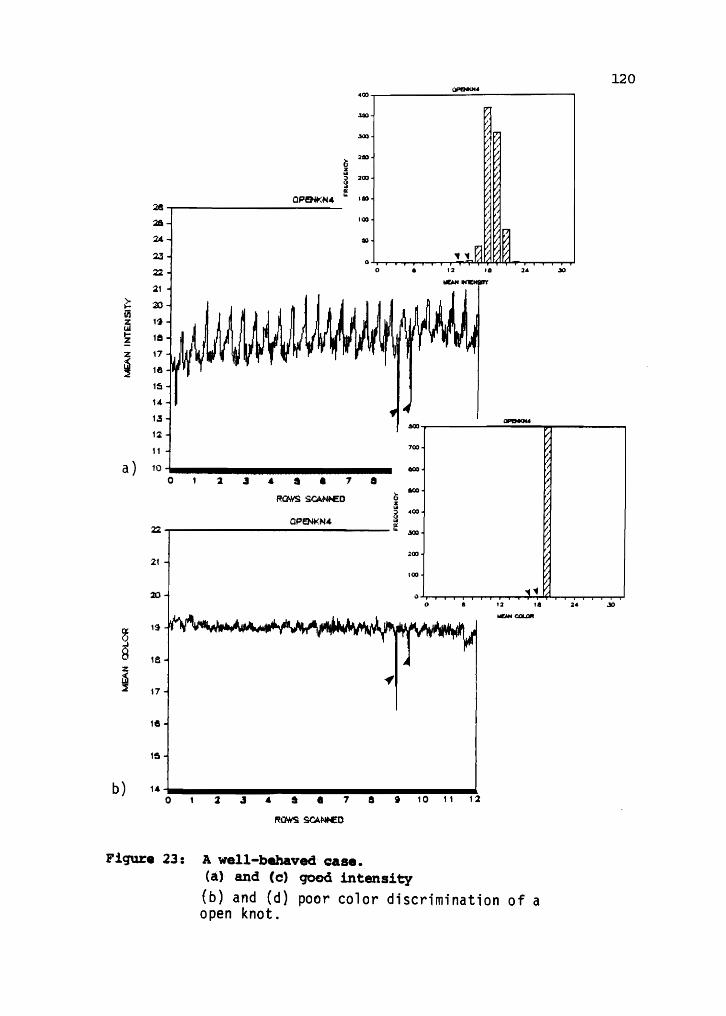
24
213
24
2.3
22
21
21 -
140 1 2 3 e 7
OPEWN4
Rain SCANOED
OPINKM4
OPB4014
12
Figure 23: A well-behaved case.and (c) good intensityand (d) poor color discrimination of a
open knot.
120
IS AtVIVA0444044~114441644fOrMr4010fMEM COLON
0 a 12 24 .30
24 JO

d)
100
OPENKNA
I 1 12 11 /13 21 24 27 30
441114111TY SM.=
4
,A40 1 2 3 4 3 8 7 8 9 10 11 12
ROMS SCANWO
OPENKN4
f y
0 .3 1 12 II II 21 24 27
COLOR Warn=
ROWS SCANOE0
Figure 23: A well-behaved case.(contd.) (a) and (c) good intensity
(b) and (d) poor color discrimination of anopen knot.
121

0
8
6
PFEIC2
PP3C2
3230
21:0
(4.04S SCAN1E0
1CO
603
433 -
130
63.
MAY Y7o , ,
12 13 24l I
10-iJ4INIENSRY
1 I r'
P1.3:2
POOC2
0 1 2 .3 4s e 78 *loll 12
Figure 24: An ill-behaved case.and (c) good intensityand (d) poor color discrimination of a
pitch pocket.
1
lllllllll lllllllla 12 13 24
me:« COLOR
122
0 1 23434zoo
ROWS SCA!.

Figure 24:
7-20C2
ROW SCANNED
4 3 a 7 8 9 tø 11 12
An ill-behaved case.
123
PRIX 2
01 .3 5 7 9 12 is taCALOR VARIANCE
(contd.) (a) and (c) good intensity(b) and (d) poor color discrimination of apitch pocket.
1 2 .3 4 a a 7 a 9 10 11 12
Row sCANNED
PPOC2
25 25 .30

6z
a) 10
21 -
18-
IT-
10
15
24 -
23 -
22 -
r'frtIM 1
1 2 3 4 5 I 7
ROMS SCANWO
14
ROWS SCAI
230
290 -
2E0
233 -
200 -
1 ao
-
io
a.
co
03 -
AO -
33
(
9.3 1
P1TC14 1
MCA IN/E31911Y
WEAN COLOR
Figure 25: An ill-behaved case.(a), (c) and (d) poor intensity and color,(b) marginal color response for a pitch streak.
21
21
124
22Patti 1

c) 00
a -
a-
5 -
3 -
2-
POWS SCANhE0
230
240
220 -
203
.
ff 1 00 .
"03
403
303
203
1 co
t
2 .3 4 5 5 7 a 9 10 11 12
PITCH t
COL3R YaRleSal
d) 0,0 1 2 3 4 5 5 7 a 9 10 11 12
RaWS Sr...4040E0
Figure 25: An ill-behaved case.(contd.) (a), (c) and (d) poor intensity and color,
(b) marginal color response for a pitch streak.
125
PITCH110
(3
3
4
1 30
1 40
1 40
I 20
9 12 13 13 21
eirsiserr vAwarca
24 27 JO
PITH/10
12 I 3 3 21 27
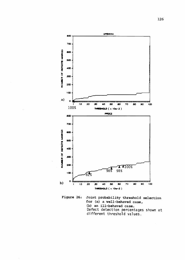
100 -
1 10 20 30 40 SO 60 70 SO 90 KO
100% THREDIOLD ( x 104r3 )
PIP00.6
b)
OPENK144,
702-
111111TIM1111111711 rn1 10 20 30 40 50 60 70
1HRESI40LO x 10,-3 )
Figure 26: Joint probability threshold selectionfor (a) a well-behaved case,(b) an ill-behaved case.Defect detection percentages shown atdifferent threshold values.
126
700-
a
200 -00%
1008
98. 98%

11. PLATES

PO' -
,
127
Plate 1.
Plate 2.
Plate 3.
- ,
::i ?Ft

LiE
EIDIE-LnD
cid 0 1='I
0
I71-orPPI1tIrViC1ED L
I. _
Plate 6.Li
"-__1=1
-
-1
,
128
Plate 4. L
.-
J
r-
Plate 5. -
c :
r- -1 -,
0
Do-
0
Lk --IL )70_EPr--
I"IVC
E

Li
1
.thr.10 - /LC - 400-. - trA16,116
Plate 7.
Plate 8.
Plate 9.
±1
_
-
-
1
LI
1
-
it ,_._, -L-1-, -
f uni :1 in 1TI
i
1
1
-
-
-- -
H
HL 129
-1
I--
Ii
_
i
__1 I _if_ L 1 _I
-
i
L.
7 -
I
AgtAN.0,-k,
tOE4.-16.5-7-
-4;
11/11/-1-1
apri-OPENKN1LI
I I tr.
1
[
k Li]
4
C:1:9
numir
LIIAm
idFT
7,61-41-1

Tm-on-PITPOC1
130i
Plate 10.
ail
Plate 11.
Plate 12.
_ -- -
,
WWI
HElL
CI91I-on-OFENKN1
"
LI
2"I
-
,
1.1.S1'1-on-CLEPRT
EllMMI111111111111111111
-
1111Ellil

Joro
EP
_L
t TI INFF1- cF11-nr_TPC1r1
_1
li0
Plate 13. L
11,
Plate 14.
Plate 15.
CI-I
1
131
rjj
I I I
TUNED-5 SiiisePENKN1 111'Er m
-1011160000.-

n_J Cl
-C
Plate 16.
Plate 18.
1
1
-
Plate 17.1
-
ni-
-
-
.Il
9r
LE I
-
e-.
-
cia_t
132
-- _
-
D-FISII-OPENKNI1uMIR
41.
I -
16,;
0giawo-w.
-wvw6"-
0 LO
Ppm Ei
n
THNIED-CISM-CLEPR7

12. BIBLIOGRAPHY
Anon. 1980. Lasers: Finding flaws, cutting waste. Wood & WoodProducts. 85(4) April.
Arnold, A. 1986. Vorteile digitaler Bildverarbeitung fur dieSpananalyse. Holz als Roh und. Werkstoff. 44:249 - 252.
Baldwin, L. 1984. Color considerations. Byte 9(10):227-246.
Ballard, D.H., C.M. Brown and J.A. Feldman. 1977. An Approach toKnowledge-directed image analysis. In: Computer Vision Systems. Eds.Allen R Hanson and Edward M. Riseman. p.271 - 281.
Ballard, D.H. and C.M. Brown. 1982. Canputer Vision. Prentice-Hall.
Brauner, A.B., and W.E. Loos. 1968. Color changes in black walnut asa function of temperature, time and two moisture conditions. For.
Prod. J. 18(5):29-34.
Brown, C.M. 1982. Color vision and Computer vision. Tech. report108. Canputer Science Department, University of Rochester, N.Y.
Cherniak, E. and D. McDermott. 1985. Introduction to ArtificialIntelligence. Addison-Wesley.
Conners, R.W., and C.A. Harlow. 1978. Equal probability quantisizingand texture analysis of radiographic images. Carputer graphics and
Image processing. Aug.
Conners, R.W., and C.A. Harlow. 1980. A theoretical comparison oftexture algorithms. IEEE Trans. on pattern analysis and machineintelligence. PAMI-2 (3) .
Conners, R.W., C.W. McMillin, K. Lin, and R.E. Vasques-Espinosa. 1983.Identifying and locating surface defects in wood: part of anautomated lumber processing system. IEEE Trans. on Pat. Anal. andMach. Intelligence. PAMI-5 (6) :573-583.
Conners, R.W., C.W. McMillin, and R.E. Vasques-Espinosa. 1984. Aprototype software system for locating and identifying surface defectsin wood. Proceedings of the 7th Int. Conf. on Pat. Recognition.Montreal, Canada. 7(1):416-419.
Conners, R.W., C.W. McMillin, and R.E. Vasques-Espinosa. 1984. Aprototype software system for locating and identifying surface defectsin wood. Pages 107-114 in Scanning Technology for the Eighties.Special Publication No. SP-21. Forintek Canada Corp., Vancouver,B.C., Canada.
133

134
Conners, R.W., C.W. McMillin, and C.N. Ng. 1985. The utility of colorinformation in the location and identification of defects in surfacedhardwood lumber. Pages XATELI-1 to wrII-33 in Proceedings of theFirst International Conference on Scanning Technology in Sawmilling.Miller Freeman Pubs., San Francisco, Ca.
Cunningham, R. 1981. Segmenting Binary Images. Robotics Age.July/Aug 4-19.
Darling, E.M, and R.D. Joseph.Satellite Altitudes. IEEE Trans.Vol SSC-4(1):38-47.
Duda, R.O., and P.E. Hart. 1973.Analysis. Wiley.
Dunbar, P. 1986. Machine Vision. Byte Jan. 161-173.
Fischer, R., W. Harbich, and K. Schick. 1985. Einsatz derMikroelektronik bei der Verarbeitung von Vollholz. Holztechnologie.26:193-196.
Fu, K-S. 1974. Syntactic methods in Pattern Recognition. AcademicPress. N.Y.
Fukada, Y. 1978. Spatial clustering procedure for region analysis.Fourth International joint conf. on Pattern Recognition.
Gray, V.R. 1961. The colour of wood and it's changes. Timberdevelopment Association Ltd. Research Report C/RR/10.
Hall, E.L. (1979). Canputer Images Processing and Recognition.Academic Press. p368-515.
Hanson, A.R. and E.M. Riseman. 1977. Segmentation of Natural Scenes.In: Computer Vision Systems. Eds. Allen R. Hanson and Edward M.Riseman. p.271 - 281.
Haralick, R.M., K. Shanmugam, and I. Dinstein. 1973. Texturalfeatures for image classification. IEEE Trans. on Systems, Man andCybernetics. SMC-3(6).
Haralick, R.M., and K. Shanmugarn. 1973. Computer classification ofreservoir sandstones. IEEE Trans. on Geosci. Electron. GE-11.
1968. Pattern recognition fromon Systems Science and Cl/ban-let:Lc&
Pattern Classification and Scene
Ho, C-S. 1983. Precision of Digital Vision Sytems. IEEE Trans. onPattern Analysis and Machine Intelligence. PAMI-5(6). November.

135
Hunter, G.M. and K. Steiglitz. 1985. Operations on Images Using QuadTrees. In: Digital Image Processing and Analysis. Vol 2. p390 - 398.Eds. Rama Chellapa and Alexander A. Sawchuck.
Ito, T., and M. Fukushima. 1976. Computer analysis of colorinformation with applications to picture processing. ThirdInternational joint conf. on Pattern Recognition.
Judd, D.B., and G. Wysecki. 1963. Color in business, Science andIndustry. Wiley N.Y.
Karonen, A. 1985. Scanning systems for automated lumber edging andtrimming. In: Proceedings of the First International Conference onScanning Technology in Swamilling. Miller Freeman Publication.
Kelly, M.D. 1971. Edge detection in pictures by computer usingplanning. Machine Intelligence 6. Elsevier, N.Y.
Kruger, R.P., W.B. Thompson, and A.F. Turner. 1974. Computerdiagnosis of pneumoconiosis. IEEE Trans. on Systems, Man andCybernetics. SMC-4(1).
Lakatosh, B.K. 1966. Defectoscopy of Wood. Translated 1970, IndianNational Scientific Documentation Center. New Delhi.
Lu, S.Y., and K-S. Fu. 1978. A syntactic approach to textureanalysis. Computer graphics and Image processing. July.
Maleta, M.V. 1984. Optimizing lumber recovery using board profile anddefect detection scanning techniques. In: Scanning Technology for theEighties. Special publication No. SP-21. Forintek Canada Corp.,Vancouver, B.C., Canada.
Marr, D. 1977. Representing Visual Information. In: Ccmputer VisionSystems. Eds. Allen R. Hanson and Edward M. Risernan. p.271 - 281.
Marr, D. 1980. Vision. Freeman Pubs.
Mathews, P.C., and B.H. Beech. 1976. Method and apparatus fordetecting Timber Defects. U.S. Patent 3976384.
Mehl horn, L., and B. P1 inke. 1985. Qua 1 itatskontro 1 1 e in derHolzwerkstoffindustrie mit hilfe digitaler Bildverarbeitung. Holz alzRd). und Werstoff. 43:403-407.
MtGinnes, E.A. 1975. Influence of incandescent and fluorescent lighton the color of unfinished heartwood of black walnut and eastern redcedar. Wood Sci. 7(4):210-279.

136
McMillin, C.W., R.W. Conners, and H.A. Huber. 1984. ALPS - Apotential new automated lumber processing system. For. Prod. J.34 (1) .
McMillin, C.W. 1982. Application of image analysis to wood science.For. Prod. J. 14(3).
Moon, P., and D.E. Spencer. 1948. The color of unstained wood.Journal of the Optical Society of America. 38(4):405-408.
Moslemi, A.A. 1969. Quantitative color characterization of loblollypine veneer. Wood Sci. 2(1):61-64.
Nelson, N.D., R.R. Maeglin, and H.E. Wahlgren. 1969. Relationship ofblack walnut color to soil properties and site. Wood and Fiber.1(1) : 29-37 .
Ohlarder, R. 1975. Analysis of natural scenes. Fh.D thesis. Dept. ofConwter Science, Carnegie-Mellon.
Ohta, Y., T. Kanade, and T. Sakai. 1980. Color information for regionsegmentation. Cc:imputer Graphics and Image Processing. 13:222-241.
Ohta, Y. (1985). Knowledge-based Interpretation of Outdoor NaturalColor Scenes. Pitman Publishing Inc.
Pratt, W.K. 1978. Digital Image Processing. Wiley.
Resch, H., E.T. Choong, and H.H. Smith. 1968. Sorting incense cedartypes for drying. For. Prod. J.:40-44.
Rosenfeld, A. 1970. Connectivity in digital pictures. Journal of theACT4 17(1): 146-160.
Rosenfeld, A. and A.C. Kak. 1982. Digital Picture Processing. 2ndEdition Vol. 1 & 2. Academic Press.
Serra, J. 1980. Image Analysis and Mathematical Morphology. AcademicPress.
Sternberg, S.R. 1979. Parallel architectures for image processing.3rd International IEEE COMPSAC. Chicago.
Sternberg, S.R. 1981. Architectures for neighborhood processing. IEEETrans. on Computer Architecture.
Sternberg, S.R. 1985. Three-dimensional machine vision. VISION 85proceedings.

137
Shibamoto, T., Y. Inoue, and Y. Kenjo. 1961. Studies on water-bornewood preservatives XVII: Color change of wood treated with colorantscaused by weathering. Journal of the Japan Wood Research Society6:122-128.
Shibamoto, T., Y. Inoue, and Y. Kenjo. 1961. Studies on water-bornewood preservatives XVIII: Color change of wood treated with colorantscaused by weathering. Journal of the Japan Wood Research Society6:147-151.
Soest, J. 1984. Optical scanning technique for defect detection.Pages 120 - 123 in Scanning Technology for the Eighties. Specialpublication No. SP-21. Forintek Canada Corp., Vancouver, B.C.,canada.
Soest, J., and P.C. Matthews. 1985. Laser scanning technique fordefect detection. Pages XVII-1 to XVII-4 in Proceedings of the FirstInternational Conference on Scanning Technology in Sawmilling. MillerFreeman Publication.
Sullivan, J.D. 1967. Color characterization of wood: spectophotometryand wood color. For. Prod. J. 17(7) :43-48.
Sullivan, J.D. 1967. Color characterization of wood: color parametersof individual species. For. Prod. J. 17(8):25-29.
Szymani, R., and K.A. McDonald. 1981. Defect detection in lumber:state of the art. For. Prod. J. 31(11):34-44.
Szymani, R. (1984). Automation in lumber defect detection. In:Scanning Technology for the Eighties. Special publication No. SP-21.Forintek Canada Corp., Vancouver, B.C., Canada.
Szymani, R. (1985). An overview of scanning technology in sawmilling.In: Proceedings of the First International Conference on ScanningTechnology in Sawmilling. Miller Freeman Publication
Teague, M.R. 1980. Image analysis via the general theory of moments.Journal of the Critical Society of America. 70(8) 920-930.
Tou, J.T., and R.C. Gonzalez. 1974. Pattern Recognition Principles.Addison-Wesley.
Webb, D.A., and J.D. Sullivan. 1964. Surface effect of light andwater on wood. For. Prod. J. 14(11):531-534.
Werman, M. and S. Peleg. 1985. Min-max operators in texture analysis.IEEE Trans. on Pat. anal. and Mach. Intelligence. PAMI-7(6).November.

138
Weszka, J.S., C.R. Dyer, and A. Rosenfeld. 1976. A comparative studyof texture measures for terrain classification. IEEE Trans. onSystems, Man, and Cybernetics. SMC-6(4).
Weszka, J.S. 1978. Survey: A survey of threshold selectiontechniques. Cmputer Graphics and Image Processing. Aug.

13 . APPENDIX

13. PERSONAL CCIMMENTS AND RECCRMENDA.TIONS
The definition and development of the image sweep and mark
algorithms extended over a period of approximately two years. Several
major conclusions and results have been formally reported in this
thesis. However, other concepts and further ideas have matured due to
personal communications, experiments, and numerous informal
discussions with colleagues. These comments are by no means
exhaustive or complete since the subject is extensive. These ideas
are reported informally for future consideration. It was necessary to
make additional references to suitable literature in this section.
These represent sane possibilities, however a more irdepth study of
the literature would be necessary when considering an extension to
this thesis.
Of the algorithms analyzed, SISM has been shown to produce the
most promising results. In fact, it may be tempting to use SISM as
the main processing routine. However, this would not be advisable.
SISM further has the possibility for being implemented on parallel
processor hardware which offers attractive prospects to machine
manufacturers.
CISM has sane potential for improvement through more extensive
cluster analysis. This possibility becomes evident when studying the
graphs of the clusters where defects are shown to appear distinctly
outside the main clustering scheme. Several good ideas to improve
CISM are discussed in Hall (1979, p375-378).
139

140
MISM did not produce the same quality of results as SISM or cISM.
Perhaps the texture measures that MISM used may not have been ideal
for wood. Conners et al. (1983) have reported a similar effect when
applying second-order statistical operators during pre-processing of
red oak lumber. Hag/ever, texture analysis may well belong to higher-
order processing. The usefulness of mathematical morphology should
also not be urderestimated, even in the light of the results of this
thesis.
The ISM algorithms developed in this thesis have only been tested
on images of wood surfaces. Such images have a very distinct
appearance. In general, the appearance is that of a homogeneous
material with defects appearing as small discontinuities. The ratio
between the discontinuities and the hanogeneous part is usually a very
small fraction (typically less than 10%).
The working premise of the algorithms is that they characterize
the homogeneous part and then use the derived characteristic to detect
small discontinuities. This premise may thus be summarized as (a)
the existence of largely homogeneous substance (b) the existence of a
unique characteristic for this homogeneous substance. If any of
these premises are invalid, the ISM algorithms are sure to fail
dramatically.
When considering ISM for any application other than veneer
plugging, it is necessary to determine whether the working premises
are still valid. If not, alternative schemes must be devised. Veneer
sorting and grading are good examples to consider. In these
141
applications, the raw wood material may be extremely variable, e.g.
may contain roundup, serious splits, lathe checks etc. Some of this
variability is caused by machining and others by log quality. For
such an application, a screening step needs to precede ISM. This
screening will serve as a crude classifier of potentially good
material from obvious trash. Once such a distinction has been made,
ISM may further be employed to determine the sort class or veneer
grade.
The veneer sorting/grading example also identifies another
important issue; resolution. The screening process described above
is concerned with gross global features arrl thus requires only very
coarse resolution. However, ISM needs a finer resolution to be able to
reliably isolate defects. A system employing a combination of high
and lad resolution offers some attractive possibilities.
It may be useful to expand on ideas of what could be done after
the ISM step. Before proceeding, let's put some aspects of machine
vision in perspective. Two broad categories of applications
associated with machine vision can be identified i.e., those in which
objects can be readily distinguished from a background, and those
where objects are fuzzy and the object/background distinction is
vague.
The first type of machine vision application is not necessarily
easy to solve, but has the potential of being solved more readily,
using well-defined methodology, i.e., image transformations,
thresholding, connectivity, mathematical morphology, statistical

142
classifiers, etc. A typical example is the "bin picking" problem.
This is where a camera peeks into a bin of parts and has to
distinguish between several objects. One problem that needs to be
solved here is that of merging edges, occluded edges, and touching
parts.
The second type of machine vision application usually concerns
more complex scenes. Hall (1979) describes scenes and images as
follaas:
"...Since most objects encountered in the physical world arethree-dimensional, a collection of these objects may be called ascene and a two-dimensional picture may be generated by viewingan image of the scene."
A scene typically contains a multitude of objects which, more often
than not, are not not clearly distinguishable from the background. In
addition the backgraind is often not clearly defined. For these type
of images, edges are generally poorly defined, may merge with other
edges, may disappear only to reappear again at a later spot, or may be
occluded. Other edges may not be formed by horrogeneous boundaries. A
typical case is where texture difference, or a psychophysical effect,
indicates an edge.
The remainder of this discussion will be centered around the
latter type of machine vision application. This type of application
has no generalized methodology, although it has been investigated
extensively both from a psychology and an Al perspective.
Applications include the analysis of natural scenes, depth perception
from stereo vision, shape frau texture, optical flow analysis to study

143
notion, image deblurring, etc.
Analysis of wood surfaces for locating defects is not as complex
as, for example, analyzing an arbitrary natural scene. This is
because images of wood surfaces deal with a limited range of species
and products (e.g. veneer, plywood, dimension lumber, etc.). The
domain thus tends to be sanewhat limited. Even further reduction of
the domain is possible when scanning for the detection of defects only
by including more rigid physical constraints about wood. The results
shown in this thesis show that the image data can be reduced by as
much as 80%.
It is no coincidence that a great deal of vision methodology is
found in Al literature. The problem of combinatorial explosion
associated with the search of a vast data domain is all the more
reason to apply sca-ne of the problem-solvirg methodology frau Al, i.e.,
the definition and implementation of concepts such as representation,
search, and control.
Representation concerns what data and associated data-structures
are necessary to solve a particular problem. It is to be expected
that the kind of information that needs to be represented depends on
what must be achieved by a specific operation. Curing the ISM process,
some very fundamental parameters are extracted from the image. The
ISM algorithms present their output as black-white "sub-images".
Haaever, it is likely that alternative representations may prove to be
wore useful in higher order processing algorithms.
One popular image-representation format in the literature is the

144
tree structure. Several forms have been implemented for image
processing applications i.e., binary, quad, or pyramid. These are all
worth ezqploring.
It was indicated earlier that the analysis of images of wood
surfaces may be classified as of the type which has poor definition of
object-to-background characteristics. This type of analysis has sane
classical examples in the literature. Several good papers are
available on the analysis of x-ray images of the human ribcage, as
well as the identification of blood and other cell types. All these
papers describe how search combined with the application of several
rhysical constraints can be carried out. These constraints could be
built into a heuristic search mechanism or alternatively be conducted
by implementing a production system where the production rules state
the different physical constraints.
Ballard and Brown (1982 p.132) describe an approach using the
so-called A-heuristic. If this search is preceded by ISM, followed
by the production of an edge map, the boundaries of defects may be
determined. Once the bounlaries are knavin it would then be a simple
matter to sample within the defect and use a Bayes classifier to
determine the actual type of defect. In this brief description, the
issues involved with edge extraction were not mentioned, and they are
not trivial. Hall (1979, p393-409) gives an example of sane of these
techniques. It is also worth looking into the method used by Kelly
(1977) for some useful ideas on the use of planning. This involves
solving a simplified version of the problem and then using the

145
solution as a guide in solving the problem in detail.
Knowledge-based scene interpretation has some definite
possibilities. Ohta (1985) presented an extensive treatise of color
and knowledge-base analysis of natural color images. The principles
he presented could, with some adaptation, be implemented to detect
defects of wood surfaces. In his book, he describes a "patchery data
structure" suitable for representing different image subregions.
Bottom-up control is used during construction of the plan, and top-
dawn control used in the production system. Ballard and Brown (1982
p.317) should also be consulted for further ideas on the
implementation of a }ram/ledge-based system.
One final concexn relates to the acquisition of optimal images of
wood surfaces. This thesis indicated the importance of the
application of color technology. Presently, color sensor technology
is dictated mainly by the requirements of the TV industry.
However, the requirements of the TV industry do not always correspond
to those for machine vision applications in forest products. For
imaging wood, the region of the visible spectrum around 580nra is of
particular importance. This makes some tube-type cameras poor
alternatives due to their biased frequency response towards the
infrared region. Certain solid-state cameras have nnre suitable
frequency responses in the blue and ultraviolet region. Clearing up
some of these unknowns would enable the acquisition of better images
and this in turn would enable more reliable analysis to be performed.
This summary may paint a formidable picture of what lies ahead

146
before a final application for the detection of defects on wood
surfaces may be possible. However, automatic defect detection using
machine vision techniques is plausible within the realm of currently
available methodology, should advances be made in the understanding of
fundamental physical phenomena and in the developxnent of innovative
hardware and software.