practiceoriented estimation of the seismic demand hazard

Practice-oriented estimation of the seismic demand hazard usingground motions at few intensity levels

Brendon A. Bradley*,†

Department of Civil and Natural Resources Engineering, University of Canterbury, Private Bag 4800, Christchurch,New Zealand

ABSTRACT

This paper examines the calculation of the seismic demand hazard in a practice-oriented manner via theuse of seismic response analyses at few intensity levels. The seismic demand hazard is a more robustmeasure for quantifying seismic performance, when seismic hazard is represented in a probabilistic for-mat, than intensity-based assessments, which remain prevalent in seismic design codes. It is illustratedthat, for a relatively complex bridge–foundation–soil system case study, the seismic demand hazard canbe estimated with sufficient accuracy using as little as three intensity measure levels that have exceedanceprobabilities of 50%, 10% and 2% in 50 years which are already of interest in multi-objectiveperformance-based design. Compared with the conventional use of the mean demand from anintensity-based assessment(s), it is illustrated that, for the same number of seismic response analyses, apractice-oriented ‘approximate’ seismic demand hazard is a more accurate and precise estimate of the‘exact’ seismic demand hazard. Direct estimation of the seismic demand hazard also provides informationof seismic performance at multiple exceedance rates. Thus, it is advocated that if seismic hazard isconsidered in a probabilistic format, then seismic performance assessment, and acceptance criteria, shouldbe in terms of the seismic demand hazard and not intensity-based assessments. Copyright © 2013 JohnWiley & Sons, Ltd.

Received 21 November 2012; Revised 28 April 2013; Accepted 3 May 2013

KEY WORDS: seismic demand hazard; multi-objective seismic performance assessment; intensity-basedassessment

1. INTRODUCTION

Earthquake-induced ground motion hazard can be prescribed in a scenario-based or probability-basedmanner [1–3]. A probabilistic representation of ground motion hazard, as conventionally computedfrom probabilistic seismic hazard analysis, comprises all potential earthquake ruptures, which pose aground motion hazard to the site considered, the likelihood of rupture occurrence and theuncertainty in the consequent ground motion at a site. The so-called seismic hazard curve, one resultof probabilistic seismic hazard analysis, provides the rate [2] (or probability [4]) of exceedance ofthe ground motion intensity measure (IM) considered. Thus, the (continuous) seismic hazard curveillustrates that all ground motion IM values in its domain can occur, although obviously some with agreater likelihood than others.

Despite the fact that a seismic hazard curve provides information for a continuum of IM values, itis common to assess seismic performance on the basis of the seismic response of the systemconsidered to ground motions conditioned on a single IM value. Such a seismic performance

*Correspondence to: Brendon A. Bradley, Department of Civil and Natural Resources Engineering, University ofCanterbury, Private Bag 4800, Christchurch, New Zealand.†E-mail: [email protected]

Copyright © 2013 John Wiley & Sons, Ltd.

EARTHQUAKE ENGINEERING & STRUCTURAL DYNAMICSEarthquake Engng Struct. Dyn. (2013)Published online in Wiley Online Library (wileyonlinelibrary.com). DOI: 10.1002/eqe.2319

assessment at a single value of the conditioning IM is referred to as an intensity-based assessmentherein. For example, current seismic design guidelines (e.g. [5–8]) prescribe seismic performancecriteria on the basis of the mean seismic demand obtained from an ensemble of ground motionsscaled to a ‘target’ (often the inappropriate uniform hazard spectrum [9, 10]) for a givenexceedance rate. However, the results of an intensity-based assessment have several fundamentallimitations for use in seismic performance assessment [11]. Firstly, by definition, the distributionof seismic demand (or so-called engineering demand parameter (EDP)) from an intensity-basedassessment, fEDP|IM(edp|imy), is conditional on ground motions with IM values of IM = imy fromthe seismic hazard curve at a desired exceedance rate (lIM(imy) = y). Thus, although the seismichazard curve directly provides information on the likelihood of a certain level of ground motionbeing exceeded (i.e. lIM(imy) = y), no direct information on the unconditional exceedance of thedemand, EDP = edp, can be obtained from fEDP|IM(edp|imy), because a specific value of EDP = edpcan be exceeded by ground motions with intensity different than IM = imy. Secondly, thedistribution of seismic demand from an intensity-based assessment, fEDP|IM(edp|imy), for an IMvalue with a given exceedance rate, lIM(imy) = y, is not unique, but is in fact a function of theparticular conditioning IM considered [12, 13].

Similar to the ground motion IM hazard, lIM, the seismic demand hazard, lEDP, directlyprovides the exceedance rate of some seismic demand metric for a continuum of values. Theseismic demand hazard is computed by integrating the ground motion IM hazard and thedistribution of seismic demand versus ground motion IM obtained from multiple IM levels. Assuch, the seismic demand hazard considers the multiple potential causal earthquake ruptures;the likelihood of rupture occurrence; uncertainty in the consequent ground motion (as containedin the ground motion IM hazard); and the uncertainty in the consequent seismic response.Furthermore, unlike intensity-based assessments, the seismic demand is independent of thechoice of the conditioning IM [12].

Because of the aforementioned conceptual benefits of the seismic demand hazard as a demand-basedmetric for seismic performance assessment, it has become increasingly utilised in earthquakeengineering research (e.g. [12–22]). Such research endeavours, however, as exemplified by the citedreferences, typically use a large number of ground motion IM levels, and ground motions per IMlevel, resulting in the requirement of hundreds, sometimes thousands, of seismic response analyses.Because such a large number of analyses are not feasible in many practical situations, it maytherefore seem that the computation of the seismic demand hazard is something reserved for onlyhigh-importance engineered structures in practice.

Attempts to simplify PBEE methodologies have been previously considered [23–29]. Suchexamples, however, consider simplified solutions of the methodologies based on analyticalidealizations. In contrast, simplified implementation of PBEE methodologies can also beconsidered via an exact solution of the governing equations, but a simplification in therequired input data. For example, Eads et al. [30] illustrated how the collapse hazard can beefficiently computed by simply reducing the number of required analyses to define thecollapse fragility curve, whereas others (e.g. [31, 32]) have utilised simplified seismic responseanalysis methods.

The aim of this paper is to examine the accuracy with which the seismic demand hazard canbe estimated using significantly fewer IM levels than those that have been considered inprevious research. The next section outlines further theoretical and practical details forcomputing the seismic demand hazard. The case study of a bridge–foundation–soil system,used to provide empirical results, is then described. Following this, the error introduced as aresult of interpolation and extrapolation of the EDP|IM relationship based on seismicresponse analyses at few IM levels is illustrated. The effect of error in the EDP|IMrelationship on the computed seismic demand hazard is then examined for a multitude ofEDPs and conditioning IMs. Finally, the errors resulting from this ‘practice-oriented’approximate calculation of the seismic demand hazard are compared with ‘worst-case’intensity-based assessments [11], which involve performing intensity-based assessments with multipleconditioning IMs in an attempt to circumvent the non-uniqueness of an intensity-based assessment witha single conditioning IM.

B. A. BRADLEY

Copyright © 2013 John Wiley & Sons, Ltd. Earthquake Engng Struct. Dyn. (2013)DOI: 10.1002/eqe

2. SEISMIC DEMAND HAZARD COMPUTATION

2.1. Theory of the demand hazard

Formally, the seismic demand hazard, lEDP(edp), provides the rate of exceedance of a specific level ofseismic demand, EDP= edp, and can be computed following the intensity-based approach from (e.g. [12])

lEDP edpð Þ ¼Z1

0

PEDPjIM edpjimð Þ dlIM imð ÞdIM

��dIM (1)

where capitalised symbols represent variables, whereas lower case symbols represent realisations of theircapitalised counterpart; PEDP|IM(edp|im) is the probability that EDP> edp given IM= im, which can beobtained directly from the probability density function, fEDP|IM(edp|im); and lIM(im) is the seismichazard curve, which provides the rate of exceedance of IM> im.

The computation of the seismic demand hazard via Equation (1) is shown graphically in Figure 1.Figure 1(a) illustrates that for each value of IM considered in the integral, the derivate of the hazardcurve is computed. The absolute value of the derivative (which is negative) is required because thehazard curve is conventionally expressed as an ‘exceedance curve’ rather than a ‘non-exceedancecurve’. Figure 1(b) illustrates that the EDP|IM relationship is obtained on the basis of performingseismic response analysis for numerous values of IM and recording the value of the EDPconsidered. It is commonly justified that the EDP|IM distribution is lognormal, and hence, for eachIM level considered, the distribution parameters (mean, m, and standard deviation, s) are obtainedvia statistical inference. To compute the value of PEDP|IM(edp|im) at IM levels other than that forwhich seismic response analyses are computed as part of the integration, some form of interpolation/extrapolation is required, as elaborated upon subsequently. Hence, as depicted graphically inFigure 1(b), it can be seen that the seismic demand hazard requires the specification of the EDP|IMrelationship over a continuum of IM values, and thus, multiple IM levels at which seismic responseanalyses are required. Figure 1(b), for example, contains the results of seismic response analyses at 11

Ground motion intensity measure, IM

Ann

ual e

xcee

danc

e ra

te,

IM

Eng

inee

ring

dem

and

para

met

er,

ED

P

Ground motion intensity measure, IM

Engineering demand parameter, EDP

Ann

ual e

xcee

danc

e ra

te,

ED

P

(a) (b)

(c)

Figure 1. Schematic illustration of the calculation of the seismic demand hazard: (a) ground motion intensitymeasure (IM) hazard, lIM(im); (b) distribution of seismic demand conditional on various intensity measure

values, fEDP|IM(edp|im); and (c) the computed seismic demand hazard, lEDP(edp).

PRACTICE-ORIENTED ESTIMATION OF THE SEISMIC DEMAND HAZARD


different IM levels (with 25 ground motions per IM level). Thus, in comparison with considering theseismic response at only a single IM level via a single intensity-based assessment, the computation ofthe seismic demand hazard in this example involves 11 times the number of seismic response analysesto be conducted (and therefore also 11 times the number of ground motion to be selected for theseanalyses). As elaborated upon subsequently, the number of IM levels, which is required for an accuratecomputation of the demand hazard, is a critical consideration and is thus the focus of this paper.

2.2. Practical computation of the seismic demand hazard

To understand the requirements for the practical computation of the seismic demand hazard viaEquation (1), it is useful to consider the six sources of error, which can occur in this computation([12], p. 1430):

(1) interpolation of the seismic hazard curve, lIM(im);(2) selection of ground motions;(3) lognormal assumption of the distribution of EDP|IM;(4) interpolation/extrapolation of the mean and variance of EDP|IM;(5) uncertainty in the mean and variance of EDP|IM due to the finite number of seismic response

analyses performed;(6) numerical approximation of the continuous demand hazard integral.

As noted by Bradley [12], error source 6 is minimised via appropriate numerical integrationalgorithms and tolerances (e.g. [33]). It should be noted that the direct numerical solution ofEquation (1) is trivial, and that because approximate analytical solutions are both inaccurate andrequire additional effort to fit idealised relationships, they are therefore not recommended forquantitative use [26]. Error sources 2 and 3 can be considered as methodology-type uncertainties.Error source 2 will be statistically insignificant if ground motions are selected appropriately usingthe generalized conditional intensity measure (GCIM) approach [9, 34]. Error source 3 is usuallynegligible as the lognormal approximation is generally appropriate for the distribution of EDP|IM (e.g. [14, 35–37]). The remaining error sources 1, 4 and 5 are therefore those that relate directly to thecomputational costs of performing the seismic hazard and seismic response analyses.

Error source 1 can be minimised if the seismic hazard curve is provided at a sufficiently largenumber of IM levels, which is practical because the computational cost of doing so is typicallyseveral orders of magnitude less than that required for performing numerous seismic responseanalyses [12]. If the seismic hazard curve is provided by an external third party (e.g. http://geohazards.usgs.gov/hazardtool/), then the analyst may not have the option of obtaining lIM(im) atmany points. However, lIM(im) is typically a ‘very smooth’ function (i.e. the first derivative changesslowly with IM), because it is the result of a probabilistic calculation with large uncertainties, andtherefore, usually a sufficient number of points are given for error source 1 to be unimportant.

Error sources 4 and 5 are the principal hindrance in the computation of the seismic demand hazard,because seismic response analyses are significantly more computationally demanding than calculationof the seismic hazard curve. In this paper, particular attention is given to the effect of error source 4resulting from the interpolation (and extrapolation) of the mean and variance of EDP|IM based onperforming seismic response analyses at only a few IM levels. To examine this error source,‘approximate’ results, based on the use of seismic response analyses at only a few IM levels, will becompared with the ‘exact’ results, based on the use of a large number of IM levels. Obviously,attention to the number of ground motion records considered at each IM level is also of importance(i.e. error source 5), but is beyond the scope of the current paper.

3. CASE STUDY CONSIDERED

To adequately assess the accuracy of the demand hazard computed using seismic response analyses at asmall number of intensity levels, it is necessary to consider a seismic response problem which isnontrivial. As such, the seismic response of a bridge–foundation–soil system in which the

B. A. BRADLEY


http://geohazards.usgs.gov/hazardtool/

http://geohazards.usgs.gov/hazardtool/

foundation soils are susceptible to liquefaction is examined here. The specific bridge–foundation–soilseismic response model considered represents the transverse direction of the Fitzgerald Avenue bridgein Christchurch, New Zealand. Several previous seismic response analysis studies have beenperformed for this structure, in both the transverse [12, 38] and longitudinal [39] directions. In thefollowing comparisons of calculated demand hazard curves, the seismic response analysis resultspresented in the work of Bradley [12] are directly utilised, and therefore, the reader is directed to thework of Bradley [12], and references therein, to obtain further detail on the geometry of the systemand the modelling of its various components.

The seismic response of the case study structure was considered via a total of 1650 seismic responseanalyses, comprising [12]:

(1) six different conditioning IMs (peak ground acceleration, peak ground velocity, 0.5-s spectralacceleration (SA(0.5)), SA(1.0), spectrum intensity (SI) and cumulative absolute velocity (CAV));

(2) 11 different IM levels for each conditioning IM (corresponding to exceedance rates with Poissonexceedance probabilities of 99%, 80%, 50%, 20%, 10%, 5%, 2%, 1%, 0.5%, 0.2% and 0.1% in50 years);

(3) 25 ground motions considered for each IM level.

Six conditioning IMs were considered to illustrate the effect of this IM choice on the results; however,in practice, analysts would utilise only a single conditioning IM. For each of the analyses considered, theseismic response of the system was quantified using a variety of EDPs [12]. Here, the analysis results forfour different EDPs will be considered: (i) the peak displacement of the ground surface in the free field,UFF; (ii) the peak displacement of the foundation pile head, UPH; (iii) the peak curvature in the pilefoundations, fP; and (iv) the peak acceleration of the bridge deck, aD.

The distribution PEDP|IM(edp|im) in Equation (1) is obtained on the basis of statistical inference of theresults from seismic response analyses. Note that global collapse of the case study structure (identified bynumerical instability in the analysis) was not observed. If global collapse is significant in other cases,PEDP|IM(edp|im) should be obtained by considering collapse and non-collapse cases separately [40].

As previously noted, it was not the intention of this paper to examine the error in the seismic demandhazard resulting from the finite number of ground motion considered for each IM level. Therefore, itshould be noted that the use of 25 ground motions per IM level is such that the resulting error in thedemand hazard is relatively small, as illustrated in the work of Bradley [12], and hence, errorsresulting from the number of IM levels can be generally considered separate from those whichwould be incurred using a smaller number of ground motions per IM level.

The seismic response analyses for the 66 different IM levels were based on ground motions selectedusing the GCIM approach [9, 34], which is explicitly consistent with the seismic hazard considered.When making the subsequent comparisons between the seismic demand metrics from intensity-based assessments and the seismic demand hazard, it is critical that both have been obtained on thebasis of a consistent method of ground motion selection. As noted by Bradley [12], consistentground motion selection ensures that the demand hazard will be statistically independent of theconditioning IM selected.

Finally, it should be noted that in addition to the uncertainty in the seismic response resulting fromground motion uncertainty, there is also uncertainty due to the idealised modelling of the system viathe adopted seismic response analysis model. This uncertainty is not directly considered herein,although the errors in the demand hazard resulting from the error in the EDP|IM relationship due to (i)ground motion or (ii) ground motion and numerical model uncertainty are likely to be similar (becausethe latter will inevitably simply result in a larger uncertainty in fEDP|IM(edp|im)). Such an assertion canbe validated in future research.

4. PARAMETRISING EDP|IM FROM SEISMIC RESPONSE ANALYSES AT A LIMITEDNUMBER OF IM LEVELS

As previously noted, computation of the seismic demand hazard requires that the EDP|IM relationshipbe prescribed over a continuum of IM values. However, in a practical context, seismic response



analyses will be performed at only a limited number of IM levels (e.g. Figure 1(b)). Thus, computationof PEDP|IM requires interpolation (and extrapolation) at all other IM values required in the demandhazard calculation.

Interpolation and extrapolation of the EDP|IM relationship, for the purposes of computing thedemand hazard, can be performed in two general ways. Firstly, the value of PEDP|IM can beobtained directly on the basis of the interpolation/extrapolation of values computed at each ofthe IM levels considered. Secondly, the parameters of the distribution, fEDP|IM (i.e. mlnEDP|IMand slnEDP|IM for a lognormal distribution), can be interpolated/extrapolated on the basis of theparameter values at each of the IM levels considered, and the value of PEDP|IM is obtainedsubsequently from the lognormal assumption. The problem with the former approach is thatPEDP|IM is difficult to interpolate/extrapolate because of the following: (i) relatively large high-order derivatives; and (ii) although PEDP|IM = [1, 0] for the limiting cases of IM = [0, 1], thesebounds are not useful in practice because such limiting cases are not of concern. For thesereasons, the second and more common approach of interpolating mlnEDP|IM and slnEDP|IM willbe considered herein.

There are various interpolation and extrapolation methods that can be used to provide estimates of afunction based on observations at a discrete set of points, such as polynomial or spline interpolation.Because the number of different IM levels that will be considered here is small, such as two or threeIM levels (as desired from a practical viewpoint), and because there is no need for continuity of firstand higher derivatives of the EDP|IM relationship, attention is restricted to piecewise linearinterpolation. The results to follow were also considered using alternative interpolation functions,with minimal differences found. Thus, simple piecewise linear interpolation is consideredappropriate for practical computation.

4.1. Interpolation and extrapolation of m lnEDP IMj

Previous parametric functions for the central tendency of the EDP|IM relationship have often been of apower model form, such that the relationship between ln(EDP) and ln(IM) is linear (e.g. [21, 24, 41]).Although it is acknowledged that such a functional form has been principally utilised because it allowsa closed-form solution of the demand hazard (and that such analytical solutions can be significantlyerroneous, as previously noted), it will be used herein for piecewise interpolation. That is, theequation for interpolation of the lognormal mean is given by

m lnEDPjIM imð Þ ¼ ln aið Þ þ bi ln imð Þ imi ⩽ im < imiþ1

bi ¼ln

miþ1

mi

� �

lnimiþ1

imi

� � ; ai ¼ exp mi � bi ln imið Þ½ � (2)

where ln() is the natural logarithm of its argument and mi is shorthand for mlnEDP|IM(imi), where imi isthe IM level at which seismic response analyses have been performed and the lognormal meancomputed. Note that the notation of the constant coefficient in the piecewise interpolation has been

kept as ln(ai) so that the median of the distribution EDP50jIM ¼ exp m lnEDPjIM imð Þ� �

¼ aiimbi .

Some extrapolation of the EDP|IM relationship may also be required if the seismic demand hazardis required for exceedance rates which are similar to the rates of the maximum and minimum IMlevels considered. Needless to say, extrapolation errors are generally larger than interpolationerrors; therefore, care should be exercised in the maximum and minimum exceedance rates of thedemand hazard, which are considered reasonable. To allow for some level of extrapolation, theinterpolation function for the first and last piecewise segments is simply extended. Figure 2(a)provides a schematic illustration of the interpolation and extrapolation of the lognormal meanseismic demand.

B. A. BRADLEY


4.2. Interpolation and extrapolation of s lnEDP IMjThe lognormal standard deviation is assumed to follow a piecewise linear variation between IM levelsin logarithmic space, given by

s lnEDPjIM imð Þ ¼ ci þ di ln imð Þdi ¼ siþ1 � si

lnimiþ1

imi

� �

ci ¼ si � di ln imið Þ

(3)

where si is shorthand notation for slnEDP|IM(imi), where imi is the IM level at which seismic responseanalyses have been performed and the lognormal standard deviation computed. For the purposes ofextrapolation, the standard deviation was taken as a constant and equal to the calculated value at themaximum or minimum IM level considered. Figure 2(b) provides a schematic illustration of theinterpolation and extrapolation of the lognormal standard deviation.

4.3. Parametric EDP|IM errors using two IM levels from case study results

To illustrate the adequacy of the parametric form of the EDP|IM relationship, it is instructive toconsider the seismic response analysis data from the case study structure for several EDP and IMcombinations. Results are firstly considered for the situation in which seismic response analyses areperformed at only two different IM levels, taken here to be those corresponding to IM exceedancerates which have 10% and 2% in 50-year exceedance probabilities. Results will also besubsequently considered for three different IM levels, where the third IM level considered is thatwhich has a 50% in a 50-year exceedance probability. These IM levels were selected because theyare commonly adopted in multi-objective performance-based design and/or assessment, with the

Figure 2. Interpolation and extrapolation of the EDP|IM relationship between IM levels at which seismicresponse analyses are performed: (a) the lognormal mean and (b) the lognormal standard deviation.



ground motion levels corresponding to these exceedance probabilities denoted as ‘Frequent’, ‘Design’and ‘Maximum Considered’ in FEMA350 [42], for example, and similar naming elsewhere [43, 44].

Figure 3 illustrates the adequacy of the parametric approximation based on two IM levels forthe relationship between peak pile curvature, fp, and either SA(0.5) (i.e. Figure 3(a–c)) or SI(i.e. Figure 3(b–d)). In Figure 3(a, b), individual seismic response analysis results are shownwith individual data points at all 11 IM levels, as well as the exact piecewise function basedon all of these 11 IM levels. Also shown is the approximate results based on using only twoIM levels. As expected, it can be seen that the error resulting from extrapolation increases asthe IM value of interest deviates from the two IM levels upon which the parametric form is based. Thisis particularly the case in Figure 3(b) for the fp–SI relationship, which can be seen to be significantlyunderpredicted based on the linear (in log–log space) approximation. Although there are differences atthe single IM level at which interpolation is performed (corresponding to an exceedance probability of5% in 50 years), it can be seen that they are minor in relation to those resulting from extrapolation.

Figure 3(c, d) illustrates the lognormal standard deviation computed at the 11 IM levels for whichseismic response analyses were performed. Also shown is the parametric approximation of thestandard deviation, which is obtained on the basis of using only two IM levels. It can be seen thatwhile the standard deviations fluctuate with IM level, they fall within a relative narrow range, incomparison with the general increase in the lognormal mean demand with increasing IM level. As aresult, it can be clearly seen in Figure 3(c, d) that the use of a constant standard deviation forextrapolation is appropriate and that the use of linear extrapolation would result in large errors, andpossibly even negative values.

With regard to bias resulting from extrapolation, it can be seen that for the fp–SA(0.5) relationship inFigure 3(a), the linear approximation for the mean results in an overprediction at small IM values,although such an approximation results in an underprediction of the fp–SI relationship in Figure 3(b).This indicates that an overprediction or underprediction in extrapolation is not a function of the EDPconsidered (both of which are fp in Figure 3(a, b)). Similarly, Figure 4(a, b) illustrates the adequacy ofthe linear approximation for two cases with the same conditioning IM (i.e. CAV), but different EDPs,with overprediction for small CAV values in Figure 4(a), but little bias in Figure 4(b). Thus, it can alsobe seen that there is no systematic overprediction or underprediction dependent on the choice of the

Figure 3. Comparison between the case study seismic response analysis results, the exact piecewise variationin distribution parameters based on all 11 IM levels and the approximate variation in distribution parametersbased on two IM levels, for the same EDP but different conditioning IMs. (a, b) illustrate the median, 16th

and 84th percentiles; (c, d) illustrate the lognormal standard deviation.

B. A. BRADLEY


conditioning IM. Hence, when seismic response analyses are performed at a limited number of IM levels,it is not possible to estimate the sign of the extrapolation error, and one can only note that the magnitude ofthe error is likely to increase with increasing extrapolation.

4.4. Parametric EDP|IM errors using three IM levels from case study results

In the previous paragraphs, it was seen that the principal problem with the parametric form for theEDP|IM relationship was based on extrapolation. Because the two IM levels considered were thoserelated to the 10% and 2% in 50-year exceedance probabilities, the extrapolation error wasparticularly large for significantly greater exceedance probabilities, which are also of relevance inseismic performance assessment. Logically, it is therefore desirable to consider the use of three IMlevels, where the third IM level considered is that corresponding to an exceedance probability of50% in 50 years.

Figure 5 illustrates the same EDP|IM plots shown in Figures 3 and 4, but with the approximateEDP|IM distribution based on three IM levels. Because the interpolation/extrapolation is piecewise,the predictions for the exceedance probabilities less than 10% in 50 years (i.e. the ‘middle’ IMlevel) are unchanged. It can be seen that the addition of the third IM level improves the piecewiseprediction for the EDP|IM distribution in all cases, particularly those in Figure 5(b, c), where theslope of the piecewise interpolation segments vary noticeably. Although figures are not explicitlyprovided for the variation in the lognormal standard deviation based on three IM levels, it can berelatively easily seen from examining Figures 3(c, d) and 4(c, d) that the addition of third IM levelswould also notably improve the parametric approximation of the standard deviation over the full IMrange of interest.

4.5. Error in parametric EDP|IM relation for all case study results

Figures 3–5 illustrated the errors associated with the piecewise approximation of the EDP|IMrelationship using seismic response analyses based on only two or three IM levels for a subset of thetotal number of 24 EDP|IM combinations (i.e. four EDPs and six conditioning IMs) that exist in thecase study data. Here, the errors for all of these EDP|IM combinations are considered to enable a

Figure 4. Comparison between the case study seismic response analysis results, the exact piecewise variationin distribution parameters based on all 11 IM levels and the approximate variation in distribution parametersbased on two IM levels, for different EDPs but the same conditioning IM. (a, b) illustrate the median and

16th and 84th percentiles; (c, d) illustrate the lognormal standard deviation.



more direct examination of the error in the mean and standard deviation. To consider multiple EDPs ina single figure, it is necessary to present the errors between the exact results (i.e. those directly obtainedon the basis of 11 IM levels) and the approximate results (i.e. those based on two or three IM levels andthen interpolated/extrapolated to other IM values) in the form of error ratios. The error ratio in themedian of the EDP|IM distribution is obtained from the ratio between the exponentials of the

lognormal means, that is, exp mobservedlnEDPjIM� �

=exp mpredictedlnEDPjIM� �

. Similarly, the error ratio in the standard

deviation of the EDP|IM distribution is obtained from sobservedlnEDPjIM=spredictedlnEDPjIM . To plot these error ratios

for different conditioning IMs, the exceedance rate of the IM level is utilised.Figure 6 illustrates the error ratios in the median and standard deviation of the EDP|IM distribution

for the 24 different EDP|IM combinations of seismic response analysis results. It can be firstly notedthat, by definition, there is no error in the median and standard deviation at the IM levels consideredin developing the piecewise interpolation/extrapolation (i.e. an error ratio of 1.0). As was noted withrespect to the subset of results shown in Figures 3 and 4, Figure 6(a) illustrates that when two IMlevels are considered, the largest error in the prediction of the median corresponds to exceedancerates significantly greater than the lower error of the two IM levels (i.e. IM values for whichlIM ≫ 10% in 50 years). At the smallest IM level considered (corresponding to a 99% in a 50-yearexceedance probability), it can be seen that the average error ratio in the median EDP|IM value isapproximately 2.5, with the 84th percentile error ratio equal to approximately 5.0. In contrast, it canbe seen that there is no significant error in the median EDP|IM when extrapolating to exceedanceprobabilities rarer than the larger error of the two IM levels considered, with the average error ratioclose to 1.0 and of relatively small variation. Partially as a result of this difference in the medianerror ratios for extrapolation above and below the two IM levels shown in Figure 6(a), it will besubsequently seen that the seismic demand hazard is very poorly predicted at exceedance ratesgreater than those corresponding to these two IM levels.

Figure 5. (a–d) Comparison between the case study seismic response analysis results, the exact piecewisevariation in distribution parameters based on all 11 IM levels and the approximate variation in distributionparameters based on three IM levels. In each subpanel, the parametric distribution is illustrated via the

median and 16th and 84th percentiles.

B. A. BRADLEY


Figure 6(b) illustrates the error ratio in the median value of the EDP|IM relationship based onconsidering seismic response analyses at three IM levels. As previously noted, because theparametric EDP|IM relationship is considered in a piecewise manner, the results in Figure 6(a, b) areidentical for IM levels with exceedance rates less than the middle of the three IM levels considered.It can be seen that the addition of the third IM level, corresponding to an exceedance rate with 50%probability of exceedance in 50 years, leads to a significant reduction in the error ratios for morefrequent exceedance rates, as compared with those based on using only two IM levels. Although not asimmediately obvious, there is also an improvement in the error ratio at an exceedance rate of 0.0044,which is based on extrapolation when using only two IM levels (Figure 6(a)), but interpolation whenusing three IM levels (Figure 6(b)).

Figure 6(c, d) illustrates the error ratios in the standard deviation of the EDP|IM relationship basedon the use of two and three IM levels, respectively. It can be seen that the use of a third IM levelreduces the error ratio in the standard deviation at more frequent exceedance rates, but the reductionis not as noticeable as that for the median in Figure 6(a, b).

5. ESTIMATION OF THE DEMAND HAZARD USING FEW IM LEVELS

Having examined the errors in the EDP|IM relationship resulting from interpolation and extrapolationto IM values other than those at which seismic response analysis was performed, it is now appropriateto directly examine the consequent errors in the demand hazard. It should be reiterated that, in theory,the demand hazard is unique, irrespective of the choice of the conditioning IM [12]. Such a result wasshown to be achievable in a practical context using the same seismic response analyses considered inthis study based on 11 IM levels [12]. It will be seen that the use of seismic response analysis from alimited number of (two or three) IM levels leads to a larger variation in the demand hazard computedon the basis of different conditioning IMs. Thus, for reference, the range of exact seismic demandhazard values based on 11 IM levels from the work of Bradley [12] will be provided for comparisonwith the results presented here based on two of three IM levels. This is because the error resultingfrom the interpolation/extrapolation of the EDP|IM relationship (referred to as error source 4previously) is the only difference between the results to follow and those of Bradley [12].

Figure 6. Error ratios in the lognormal mean and standard deviation of the parametricEDP|IM distribution for all24 EDP|IM combinations in the case study results for (a, c) two IM levels and (b, d) three IM levels. The differentIM levels are denoted by their hazard exceedance rate to plot different conditioning IMs on the same axis.



5.1. Demand hazard estimation using two IM levels

Figure 7(a, c) illustrates the estimation of the seismic demand hazard for peak pile curvature, fp, and peakdeck acceleration, aD, respectively, based on using seismic response analyses at only two IM levels(corresponding to 10% and 2% exceedance in 50 years). For comparative purposes, the exceedancerates of the two IM levels in parametrising the EDP|IM relationship are shown, as well as the range ofthe exact seismic demand hazard computed on the basis of using 11 IM levels[12]. Figure 7(b, d)illustrates the error ratios in the computed demand hazard EDP values for a given exceedance rate, thatis, Error ratio in EDP= edpexact/edpapprox, where lexactEDP edpexactð Þ ¼ lapproxEDP edpapproxð Þ.

Figure 7 illustrates that, as expected, the error in the estimation of the demand hazard is smallest forexceedance rates in the vicinity of those IM levels which the EDP|IM relationship is developed from.The errors in the demand hazard for exceedance rates greater than l = 2.1 * 10� 3 (i.e. corresponding to10% in 50 years) can be seen to increase drastically with increasing exceedance rate, with error ratiosexceeding factors of 0.5 or 2.0 in several cases. With reference to the errors in the EDP|IM resultspreviously discussed, it can be seen that (i) the extrapolation of the EDP|IM relationship for fp|CAV(i.e. Figure 4(b)) was fortuitously very accurate, thus resulting in a computed demand hazard, whichis similar to the exact values and (ii) in contrast, the extrapolation of the EDP|IM relationship for fp|SI(i.e. Figure 3(b)) was very underconservative, resulting in a significant underprediction of the demandhazard for a given exceedance rate. At the exceedance rates equal to the two IM levels considered, itcan be seen that generally the error ratios are within the range of [0.7, 1.3]. It can also be seen that this

Figure 7. Illustration of the computed seismic demand hazard for two EDPs based on considering seismicresponse analyses at only two IM levels. The range in the exact results based on considering seismic

response analyses at 11 IM levels [12] is also shown for reference.

B. A. BRADLEY


range in error ratio at these two exceedance rates is notably greater than that which results from the use ofseismic response analyses at 11 IM levels, illustrating the importance of accuracy in the EDP|IMrelationship over a range of IM values, when performing integration, as required in Equation (1). Thegreater error ratios in the median EDP|IM relationship for frequent exceedance rates (i.e. Figure 6(a)),combined with the fact that the contribution toward the demand hazard integral comes principally fromvalues of IM values below the median ([26], Figure 4), is a reason the error ratios for the IM levelcorresponding the 10% in 50 years are generally greater than those at the IM level corresponding to 2%in 50 years.

5.2. Demand hazard estimation using three IM levels

Figure 8 illustrates the estimation of the seismic demand hazard, and associated error ratios, for peakpile curvature, fp, and peak deck acceleration, aD, based on using seismic response analyses at threeIM levels (corresponding to 50%, 10% and 2% exceedance in 50 years). By comparing Figures 7and 8, it is immediately apparent that the inclusion of the third IM level, corresponding to 50%exceedance in 50 years, results in a significant increase in the accuracy of the computed demandhazard at frequent exceedance rates. In addition, as a result of adding a third IM level, there is also areduction in the error ratios at exceedance rates corresponding to the remaining two IM levels,with error ratios at these levels now generally within [0.8, 1.2] (in contrast to an error ratio range of[0.7, 1.3] from using only two IM levels as given in Figure 7). It can be seen in Figure 8(b, d) that

Figure 8. Illustration of the computed seismic demand hazard for two EDPs based on considering seismicresponse analyses at only three IM levels. The range in the exact results based on considering seismic

response analyses at 11 IM levels [12] is also shown for reference.



for all exceedance rates within the range of the three IM levels considered (i.e. between ratescorresponding to 50% and 2% probabilities of exceedance in 50 years), the error ratios are in therange [0.8, 1.2]. Naturally, the error ratios increase for extrapolation of the demand hazard beyondthe range of the IM levels considered, although the error does not increase rapidly, indicating that alimited amount of extrapolation may be acceptable (particularly to lower exceedance rates).

5.3. Error in the demand hazard for all case study results

Figures 7 and 8 illustrate the error ratios in the computation of the demand hazard for two differentEDPs. Figure 9 illustrates the error ratios in the demand hazard as a function of exceedance rate, forall four EDPs considered in the case study structure. With a total of six conditioning IMs, theconsideration of four EDPs gives a total of 24 error ratios per exceedance rate. The mean values,16th and 84th percentiles of the error ratios, based on the use of two of three IM levels, are alsogiven in the respective figures. For comparative purposes, the exceedance rates of the IM levels in

Figure 9. Error ratios in the computed seismic demand hazard for all 24 EDP and conditioning IMcombinations of the case study results: (a) using two IM levels and (b) using three IM levels. Therange and 16th and 84th percentiles of the exact results based on considering seismic response analyses at

11 IM levels [12] are also shown for reference.

B. A. BRADLEY


parametrising the EDP|IM relationship are shown, as well as the error ratio range and 16th and 84thpercentiles of the error ratios from the exact seismic demand hazard computed on the basis of using11 IM levels [12]. As noted with respect to Figure 7, it can be seen in Figure 9(a) that there is asignificant error in the demand hazard for exceedance rates greater than the 10% in a 50-yearexceedance probability. Furthermore, even the error in the value of the demand hazard for the10% in a 50-year exceedance probability is relatively large, with error ratios in the range[0.7, 1.3], in comparison with a range of [0.9, 1.1] based on exact results. Figure 9(b) illustratesthat the addition of a third IM level at an exceedance rate corresponding to 50% probability ofexceedance in 50 years leads to a significant reduction in the demand hazard error ratio for thesefrequency exceedance rates and also provides a further reduction in the error ratios at smallerexceedance rates. Examination of the error ratio range, and the 16th and 84th percentile values ofthe error ratio, for exceedance rates between 50% and 2% probability of exceedance in 50 years,illustrates that there is in fact no overly significant difference between those based on three IMlevels and the exact results based on 11 IM levels for exceedance rates ‘within’ those of the IMlevels considered.

Because multi-objective performance-based seismic design/assessment is often concerned with theground motion levels corresponding to at least three different exceedance rates (e.g. denoted asFrequent, Design and Maximum Considered ground motion levels in FEMA350 [42]), and becauseof the notable reduction in the error in estimating the demand hazard values using three IM levelscompared with two IM levels, it is concluded that at least three IM levels should be considered fordemand hazard estimation in a practical setting.

6. COMPARISON OF APPROXIMATE DEMAND HAZARD WITH WORST-CASEINTENSITY-BASED ASSESSMENTS

Seismic performance criteria in contemporary seismic design guidelines (e.g. [5–8]) are currently basedon the mean seismic demand obtained from an intensity-based assessment (i.e. ground motionsconditioned on a single IM value). However, the distribution of seismic demand from an intensity-based assessment, for an IM value with a given exceedance rate, is not unique but is in fact a functionof the particular conditioning IM considered [12, 13]. It has therefore been suggested (e.g. [13], Section4.2.3) that one approach could be to ensure that the seismic performance is satisfactory for seismicresponse analyses utilising ground motion ensembles based on different conditioning IMs [11]. Thislogic is analogous to the consideration of different load combinations in conventional gravity designand essentially results in the seismic demand metric being the maximum of the mean seismic demandsfrom the various intensity-based assessments considered, which will be referred to herein as a worst-

case intensity-based assessment, and denoted as max mEDPjIM¼imy

h i[11]. Given the aforementioned

benefits of the seismic demand hazard metric over those based on an intensity-based assessment, it is ofinterest to compare the accuracy and precision of the seismic demand metric obtained from a worst-case intensity-based assessment and from direct estimation of the seismic demand hazard using few IMlevels, with the exact seismic demand hazard based on numerous IM levels.

Bradley [11] recently compared the seismic demands obtained from worst-case intensity-basedassessments with the exact seismic demand hazard for the same case study structure examined here.The worst-case intensity-based assessments were performed with ground motions having an IMvalue with a given exceedance rate, l(imy) = y, and compared with the value of the seismic demandhazard for the same exceedance rate, that is, lEDP (edpy) = y. Using the notation in the work ofBradley [11], the error ratio between the EDP value from the exact seismic demand hazard, edpexacty ,

and from the worse-case intensity-based assessment, max mEDPjIM¼imy

h i, is given by

R IM-basededp ¼ edp exact

y

max mEDPjIM¼imy

h i (4)



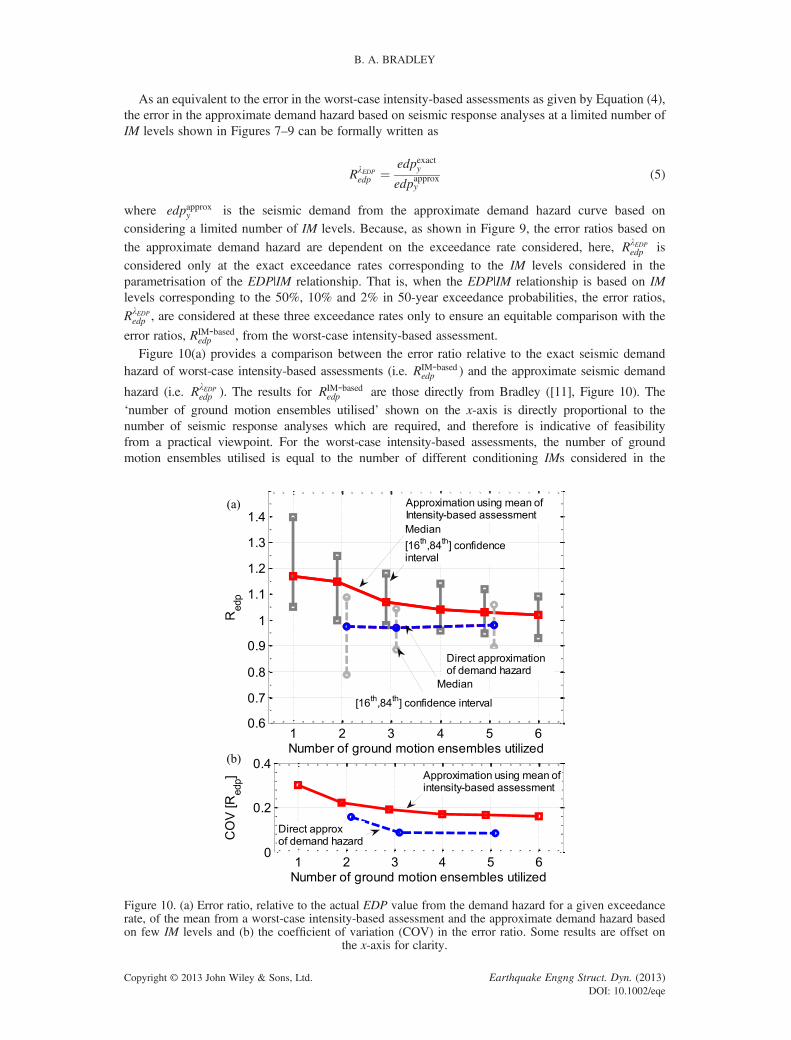
As an equivalent to the error in the worst-case intensity-based assessments as given by Equation (4),the error in the approximate demand hazard based on seismic response analyses at a limited number ofIM levels shown in Figures 7–9 can be formally written as

RlEDPedp ¼ edpexacty

edpapproxy(5)

where edpapproxy is the seismic demand from the approximate demand hazard curve based onconsidering a limited number of IM levels. Because, as shown in Figure 9, the error ratios based on

the approximate demand hazard are dependent on the exceedance rate considered, here, RlEDPedp is

considered only at the exact exceedance rates corresponding to the IM levels considered in theparametrisation of the EDP|IM relationship. That is, when the EDP|IM relationship is based on IMlevels corresponding to the 50%, 10% and 2% in 50-year exceedance probabilities, the error ratios,

RlEDPedp , are considered at these three exceedance rates only to ensure an equitable comparison with the

error ratios, RIM-basededp , from the worst-case intensity-based assessment.

Figure 10(a) provides a comparison between the error ratio relative to the exact seismic demandhazard of worst-case intensity-based assessments (i.e. RIM-based

edp ) and the approximate seismic demand

hazard (i.e. RlEDPedp ). The results for RIM-based

edp are those directly from Bradley ([11], Figure 10). The‘number of ground motion ensembles utilised’ shown on the x-axis is directly proportional to thenumber of seismic response analyses which are required, and therefore is indicative of feasibilityfrom a practical viewpoint. For the worst-case intensity-based assessments, the number of groundmotion ensembles utilised is equal to the number of different conditioning IMs considered in the

Figure 10. (a) Error ratio, relative to the actual EDP value from the demand hazard for a given exceedancerate, of the mean from a worst-case intensity-based assessment and the approximate demand hazard basedon few IM levels and (b) the coefficient of variation (COV) in the error ratio. Some results are offset on

the x-axis for clarity.

B. A. BRADLEY


intensity-based assessment. For the approximate demand hazard, the number of ground motion ensemblesutilised is equal to the number of different IM levels, which are considered in parametrising the EDP|IMrelationship. It can be seen that, for a given number of seismic response analyses required, the medianerror ratio is consistently closer to 1.0 based on the direct approximation of the demand hazard with alimited number of IMs, as compared with that based on a worst-case intensity-based assessment.Furthermore, the variability in the error ratio, as indicated by the 16th and 84th percentile confidenceinterval in Figure 10(a), or the coefficient of variation in Figure 10(b), is also smaller when directlyestimating the seismic demand hazard. The greater accuracy and precision of the direct approximationof the seismic demand hazard is apparent whether it be two, three or five ground motion ensembles,which are required for seismic response analyses. Although the precision of the direct approximation ofthe seismic demand hazard notably improves on the basis of using three IM levels in comparison withtwo (as elaborated upon previously), it can be seen that there is a diminishing return in the increasedprecision when using five IM levels (which were taken to be those with 50%, 20%, 10%, 5% and 2%probability of exceedance in 50 years). The principal reason for this is the finite sample uncertainty inthe distribution parameters of the EDP|IM relationship (i.e. mlnEDP|IM and slnEDP|IM), due to the use of25 ground motions for each IM level (e.g. [12], Figure 12).

The aforementioned results and discussion indicates that for a given number of seismic responseanalyses, it is better to directly approximate the seismic demand hazard and obtain the EDP valuefor a given exceedance rate than to utilise a worst-case intensity-based assessment. In addition tobeing more accurate and precise, it is also critical to understand that in estimating the seismicdemand hazard, more information is provided about the seismic performance. For example, if aworst-case intensity-based assessment is performed using three different ground motion ensembles(selected on the basis of three different conditioning IMs), then this assessment will provide aseismic performance metric at the single exceedance rate for which the ground motions areconsidered. In contrast, in the direct approximation of the seismic demand hazard, a singleconditioning IM is considered, seismic response analyses are performed on the basis of groundmotions selected at three different IM levels and the seismic demand hazard provides a seismicperformance metric for at least the three exceedance rates considered (which can be interpolated andeven slightly extrapolated as shown in Figure 9 and related text). Furthermore, if seismicperformance metrics based on a worst-case intensity-based assessment were required at threedifferent IM levels, then this would in fact require three times the number of seismic responseanalyses as direct approximation of the seismic demand hazard. Thus, for a given number of seismicresponse analyses, direct estimation of the seismic demand hazard for seismic performanceassessment should be preferred in comparison with the use of a worst-case intensity-based assessment.

7. CONCLUSIONS

This paper has examined the computation of the seismic demand hazard from a practical perspective,with particular focus on the error introduced via the use of seismic response analyses performed at onlya few IM levels. A case study of a bridge–foundation–soil system was used to provide empirical resultsto illustrate the salient features of the problem. The error in the relationship between the seismicdemand and ground motion intensity, as a result of interpolation and extrapolation from the IMlevels at which seismic response analyses are performed, was examined, from which it was seen thatextrapolation is the principal problem. It was seen that, for the case study considered, estimation ofthe seismic demand hazard based on two IM levels, with IM exceedance probabilities of 10% and2% in 50 years, can produce approximate results within 30% error for similar exceedance rates, buterrors in excess of a factor of 2 when extrapolated to more frequent exceedance rates that are often ofinterest. The computation of the demand hazard using seismic response analyses at three IM levels,with exceedance probabilities of 50%, 10% and 2% in 50 years, provided an estimate of the seismicdemand hazard with error ratios within 20% or less over a wide range of exceedance rates of interest.

Compared with the conventional use of the mean demand from an intensity-based assessment(s), itwas illustrated that for the same number of seismic response analyses, the seismic demand valueobtained from a practice-oriented approximate seismic demand hazard is a more accurate and



precise estimate of that from the exact seismic demand hazard. Direct estimation of the seismic demandhazard also provides information of seismic performance at multiple exceedance rates, in contrast to asingle intensity-based assessment. Thus, if seismic hazard is considered in a probabilistic format, thenseismic performance assessment, and acceptance criteria, should be in terms of the seismic demandhazard and not intensity-based assessments.

ACKNOWLEDGEMENT

Constructive comments from Dr Matjaz Dolsek (University of Ljubljana) are greatly appreciated.

REFERENCES

1. Kramer SL. Geotechnical Earthquake Engineering. Prentice-Hall: Upper Saddle River, NJ, 1996; 653.2. McGuire RK. Probabilistic seismic hazard analysis: early history. Earthquake Engineering and Structural Dynamics

2008; 37:329–338. DOI: 10.1002/eqe.765.3. Bommer JJ. Deterministic vs. probabilistic seismic hazard assessment: an exaggerated and obstructive dichotomy.

Journal of Earthquake Engineering 2002; 6(1 supp 1):43–73.4. Field EH, Gupta N, Gupta V, Blanpied M, Maechling P, Jordan TH. Hazard calculations for the WGCEP-2002

forecast using OpenSHA and distributed object technologies. Seismological Research Letters 2005; 76:161–167.5. ASCE/SEI 7-05. Minimum design loads for buildings and other structures. American Society of Civil Engineers,

ASCE Standard No. 007-05, 2006; 388pp.6. CEN. Eurocode 8: design of structures for earthquake resistance. Part 1: General rules, seismic actions and rules for

buildings, Final Draft prEN 1998, European Committee for Standardization, 2003; pp.7. FEMA-368. NEHRP recommended provisions for seismic regulations for new buildings and other structures, 2000

Edition. Part 1: Provisions, Building Seismic Safety Council for the Federal Emergency Management Agency, 2001; pp.8. NZS 1170.5. Structural design actions, Part 5: earthquake actions - New Zealand. Standards New Zealand: Wellington,

New Zealand, 2004; 82.9. Bradley BA. A generalized conditional intensity measure approach and holistic ground motion selection. Earthquake

Engineering and Structural Dynamics 2010; 39(12):1321–1342. DOI: 10.1002/eqe.995.10. Baker JW, Cornell CA. Spectral shape, record selection and epsilon. Earthquake Engineering and Structural Dynamics

2006; 35(9):1077–1095.11. Bradley BA. A comparison of intensity-based distributions and the seismic demand hazard for seismic performance

assessment. Earthquake Engineering and Structural Dynamics 2013 (submitted).12. Bradley BA. The seismic demand hazard and importance of the conditioning intensity measure. Earthquake

Engineering and Structural Dynamics 2012; 41(11):1417–1437. DOI: 10.1002/eqe.2221.13. NIST. Selecting and scaling earthquake ground motions for performing response-history analyses. NIST GCR

11-917-15, 2011; pp. 256.14. Shome N, Cornell CA. Probabilistic Seismic Demand Analysis of Nonlinear Structures, Stanford University, 1999;

pp. 357.15. Tothong P, Luco N. Probabilistic seismic demand analysis using advanced ground motion intensity measures.

Earthquake Engineering and Structural Dynamics 2007; 36(13):1837–1860.16. Jalayer F, Beck JL. Effects of two alternative representation of ground-motion uncertainty on probabilistic seismic

demand assessment of structures. Earthquake Engineering and Structural Dynamics 2007. DOI: 10.1002/eqe.745.17. Bazzurro P. Probabilistic seismic demand analysis, Stanford University, 1998; 329pp.18. Kramer SL, Mitchell RA. Ground motion intensity measures for liquefaction hazard evaluation. Earthquake Spectra

2006; 22(2):413–438.19. Bradley BA, Dhakal RP, Cubrinovski M, MacRae GA. Prediction of spatially distributed seismic demands in

structures: from structural response to loss estimation. Earthquake Engineering and Structural Dynamics 2009;39(6):591–613. DOI: 10.1002/eqe.955.

20. Rathje EM, Saygili G. Probabilistic seismic hazard analysis for the sliding displacement of slopes: scalar and vectorapproaches. Journal of Geotechnical and Geoenvironmental Engineering 2008; 134(6):804–814. DOI: 10.1061/(ASCE)1090-0241(2008)134:6(804).

21. Aslani H, Miranda E. Probability-based seismic response analysis. Engineering Structures 2005; 27(8):1151–1163.22. Krawinkler H, Miranda E. Performance-based Earthquake Engineering. Earthquake Engineering: From Engineering

Seismology to Performance-based Engineering, Bozorgnia Y, Bertero VV (eds). CRC Press: Boca Raton, FL, 2004.23. Zareian F, Krawinkler H. Assessment of probability of collapse and design for collapse safety. Earthquake Engineering

and Structural Dynamics 2007; 36(13):1901–1914.24. Mackie KR, Stojadinovic B. Performance-based seismic bridge design for damage and loss limit states. Earthquake

Engineering and Structural Dynamics 2007; 36(13):1953–1971. DOI: 10.1002/eqe.699.25. Baker JW, Cornell CA. Uncertainty Specification and Propagation for Loss Estimation Using FOSM Method,

2003; pp. 100.26. Bradley BA, Dhakal RP. Error estimation of closed-form solution for annual rate of structural collapse. Earthquake

Engineering and Structural Dynamics 2008; 37(15):1721–1737.

B. A. BRADLEY


27. Bradley BA, Lee DS. Accuracy of approximate methods of uncertainty propagation in loss estimation. StructuralSafety 2009; 32(1):13–24. DOI: 10.1016/j.strusafe.2009.04.001.

28. Dol�sek M, Fajfar P. Simplified probabilistic seismic performance assessment of plan-asymmetric buildings.Earthquake Engineering and Structural Dynamics 2007; 36(13):2021–2041. DOI: 10.1002/eqe.697.

29. Fajfar P, Dol�sek M. A practice-oriented estimation of the failure probability of building structures. EarthquakeEngineering and Structural Dynamics 2012; 41(3):531–547. DOI: 10.1002/eqe.1143.

30. Eads L, Miranda E, Krawinkler H, Lignos DG. An efficient method for estimating the collapse risk of structures inseismic regions. Earthquake Engineering and Structural Dynamics 2013; 42(1):25–41. DOI: 10.1002/eqe.2191.

31. Dol�sek M. Simplified method for seismic risk assessment of buildings with consideration of aleatory and epistemicuncertainty. Structure and Infrastructure Engineering 2012; 8(10):939–953. DOI: 10.1080/15732479.2011.574813.

32. Fragiadakis M, Vamvatsikos D. Fast performance uncertainty estimation via pushover and approximate IDA.Earthquake Engineering and Structural Dynamics 2010; 39(6):683–703. DOI: 10.1002/eqe.965.

33. Bradley BA, Lee DS, Broughton R, Price C. Efficient evaluation of performance-based earthquake engineeringequations. Structural Safety 2009; 31(1):65–74. DOI: 10.1016/j.strusafe.2008.03.003.

34. Bradley BA. A ground motion selection algorithm based on the generalized conditional intensity measure approach.Soil Dynamics and Earthquake Engineering 2012; 40(0):48–61. DOI: 10.1016/j.soildyn.2012.04.007.

35. Aslani H, Miranda E. Fragility assessment of slab-column connections in existing non-ductile reinforced concretebuildings. Journal of Earthquake Engineering 2005; 9(6):777–804.

36. Bradley BA, Dhakal RP, Cubrinovski M, MacRae GA. Prediction of spatially distributed seismic demands instructures: ground motion and structural response. Earthquake Engineering and Structural Dynamics 2009;39(5):501–520. DOI: 10.1002/eqe.954.

37. Ramirez CM, Miranda E. Building-specific loss estimation methods and tools for simplified performance-basedearthquake engineering, Stanford University, Blume Centre report number 171, 2009; pp. 370.

38. Bowen H, Cubrinovski M. Effective stress analysis of piles in liquefiable soil: a case study of a bridge foundation.Bulletin of the New Zealand Society for Earthquake Engineering 2008; 41(4):247–262.

39. Bradley BA, Cubrinovski M, Dhakal RP, MacRae GA. Probabilistic seismic performance and loss assessment of abridge–foundation–soil system. Soil Dynamics and Earthquake Engineering 2009; 30(5):395–411. DOI: 10.1016/j.soildyn.2009.12.012.

40. Shome N, Cornell CA, Bazzurro P, Carballo JE. Earthquakes, records, and nonlinear responses. Earthquake Spectra1998; 14(3):469–500.

41. Cornell CA, Jalayer F, Hamburger RO, Foutch DA. Probabilistic basis for 2000 SAC federal emergency manage-ment agency steel moment frame guidelines. Journal of Structural Engineering 2002; 128(4):526–533.

42. FEMA-350. Recommended seismic design criteria for new steel moment-frame buildings, SAC Joint Venture, 2000; pp.43. SEAOC. Vision 2000: a framework for performance-based design, Structural Engineers Association of

California, 1995; pp.44. ATC-40. Seismic evaluation and retrofit of concrete buildings, Volume 1, 1996; pp.



practiceoriented estimation of the seismic demand hazard

Documents