practical issues in implementing and understanding ...gelman/research/published/171.pdf ·...

Advance Access publication March 1, 2005 Political Analysis (2005) 13:171–187

doi:10.1093/pan/mpi010

Practical Issues in Implementing and UnderstandingBayesian Ideal Point Estimation

Joseph BafumiDepartment of Political Science, Columbia University, New York, NY

e-mail: [email protected]

Andrew GelmanDepartment of Statistics and Department of Political Science,

Columbia University, New York, NYe-mail: [email protected], www.stat.columbia.edu/;gelman/

David K. ParkDepartment of Political Science, Washington University, St. Louis, MO


Noah KaplanDepartment of Political Science, University of Houston, Houston, TX


Logistic regression models have been used in political science for estimating ideal points of

legislators and Supreme Court justices. These models present estimation and identifiability

challenges, such as improper variance estimates, scale and translation invariance, reflection

invariance, and issues with outliers. We address these issues using Bayesian hierarchical

modeling, linear transformations, informative regression predictors, and explicit modeling for

outliers. In addition, we explore new ways to usefully display inferences and check model fit.

1 Introduction

1.1 Background

Estimates of legislators’ and justices’ revealed voting preferences have become an

important resource for scholars of legislatures and courts. The most influential method

for ideal point estimation1 in political science was developed by Poole and Rosenthal

(1997). Their procedure for scoring American legislators, named NOMINATE (nominal

171

Political Analysis Vol. 13 No. 2, � The Author 2005. Published by Oxford University Press on behalf of the Society forPolitical Methodology. All rights reserved. For Permissions, please email: [email protected]

Authors’ note: The authors thank Ernesto Calvo, Simon Jackman, Eric Loken, and two anonymous reviewers fortheir useful comments. We thank the National Science Foundation for grant SES-0318115.1An individual’s ‘‘ideal point’’ refers to his or her preferences or capacities within a spatial framework. Thesimplest and most common spatial framework is characterized by a single dimension. Within a political context,this dimension is often conceived of as an ideological continuum, a line whose left end is understood to reflect anextremely liberal position and whose right end corresponds to extreme conservatism. In this one-dimensionalspatial model, any person’s ideological disposition/preference can be depicted by a point on this line—theperson’s ideal point.

http://www.stat.columbia.edu/~gelman/

three-step estimation), has revolutionized congressional research in the American

politics literature.2

In the past few years, political scientists have begun using an alternative approach for

ideal point estimation, borrowing from the extensive psychometrics literature on logistic

regression (Jackman 2000; Clinton et al. 2004). They perform these analyses using

Bayesian techniques to aid in identification and recast parameter estimation into straight-

forward missing data problems (as has been shown in the political science context by

Jackman (2000).3 Although this model offers a number of advantages relative to

NOMINATE, it also poses a number of substantive and statistical issues. In this paper we

seek to clarify these issues and suggest approaches to addressing the problems they pose.

1.2 The basic model with ability and difficulty parameters

We begin with the model as it has been understood and developed for education research

(Rasch 1980). A standard model for success or failure in testing situations is the logistic

item-response model, also called the Rasch model. Suppose J persons are given a test with

K items, with yjk ¼ 1 if the response is correct. Then the logistic model can be written as

Prðyjk ¼ 1Þ ¼ logit�1ðaj � bkÞ; ð1Þ

with parameters.4

� aj: the ability of person j

� bk: the difficulty of item k.

In general, not every person needs to receive every item, so it is convenient to index the

individual responses as i ¼ 1, . . . , n, with each response i associated with a person j(i) and

item k(i). Thus model (1) becomes

Prðyi ¼ 1Þ ¼ logit�1ðajðiÞ � bkðiÞÞ: ð2Þ

Figure 1 illustrates the model as it might be estimated for five persons with abilities aj

and ten items with difficulties bk. In this particular example, questions 5, 3, and 8 are easy

(relative to the abilities of the persons in the study), and all persons except person 2 are

expected to answer more than half the items correctly. More precise probabilities can be

calculated using the logistic distribution: for example, a2 is 2.4 higher than b5, so the

probability that person 2 correctly answers item 5 is logit�1(2.4) ¼ 0.92, or 92%.

1.3 Interpretation as an ideal point model

The Rasch model can be directly used for ideal point estimation in political science

research. Here subscript j denotes a legislator or justice and subscript k denotes a bill or

case. The ability parameter, aj, measures the liberalness or conservativeness of a legislator

2For a list of many of these works see Clinton et al. (2003).3The use of Bayesian logistic regression to estimate ideal points has become increasingly popular in the politicalscience literature. Martin and Quinn (2001, 2002b,a), Clinton et al. (2004), and Bafumi et al. (2002) have usedBayesian ideal point estimation to scale Supreme Court justices; Clinton et al. (2004) estimate ideal points in theU.S. House; and Jackman (2001), Clinton (2001), and Park (2001) employ estimated ideal points for senators.

4We use ‘‘logit�1’’ to indicate the inverse logistic function, logit�1(x) ¼ ex/(1 þ ex).

172 Joseph Bafumi et al.

and the difficulty parameter, bk, indicates the ideal point of a legislator who is indifferent

on that bill or case. Thus, in Figure 1, a4 and a5 could represent highly conservative

justices (e.g., Scalia and Thomas) and b2 would represent a case for which justice 4 would

be nearly indifferent. Justice 4 would be more likely to vote in the conservative direction

as a case’s difficulty parameter moves to the left.

From an ideal point perspective, Figure 1 illustrates a one-dimensional spatial voting

model, with the negative and positive ends of the spectrum corresponding to left-wing and

right-wing views. The logistic regression can be derived from a random utility model in

which positions are preferred if they are closer in this space; the model thus has

a theoretical as well as a statistical justification (Clinton et al. 2004). The model can be

generalized to multidimensional utility spaces by adding terms within the logistic model.

(For more on multidimensional item response models, see Rivers 2003.)

2 Identifiability problems

2.1 Additive aliasing

This model is not identified, whether written as (1) or as (2), because a constant can be

added to all the abilities aj and all the difficulties bk, and the predictions of the model will

not change. The probabilities depend only on the relative positions of the ability and

difficulty parameters. For example, in Figure 1, the scale could go from �104 to �96

rather than �4 to 4, and the model would be unchanged—a difference of 1 on the original

scale is still a difference of 1 on the shifted scale.

From the standpoint of classical logistic regression, this nonidentifiability is a simple

case of collinearity and can be resolved by constraining the estimated parameters in some

way: for example, setting a1 ¼ 0 (that is, using person 1 as a ‘‘baseline’’), setting b1 ¼ 0

(so that a particular item is the comparison point), constraining the aj’s to sum to 0, or

constraining the bj’s to sum to 0. A multilevel model allows for other means of solving the

additive aliasing problem, as we discuss next.

2.1.1 Multilevel model

Item-response and ideal point models are inherently applied to multilevel structures, with

data nested within persons and test items, or judge’s decisions, or legislator’s votes.

Fig. 1 Illustration of the logistic item-response (Rasch) model, Pr(yi ¼ 1) ¼ logit�1(aj(i) � bk(i)), for

an example with five persons j (with abilities aj) and ten items k (with difficulties bk). If your ability

a is greater than the difficulty b of an item, then you have a better-than-even chance of getting that

item correct. This graph also illustrates a nonidentifiability in the model: the probabilities depend

only on the relative positions of the ability and difficulty parameters; thus, a constant could be added

to all the aj’s and all the bk’s, and the model would be unchanged. One way to resolve this

nonidentifiability is to constrain the aj’s to have mean 0. Another solution is to give the aj’s

a distribution with mean fixed at 0. The model has other nonidentifiabilities, as discussed in the text.

173Implementing and Understanding Bayesian Ideal Point Estimation

A commonly used multilevel model for (2) assigns normal distributions to the ability and

difficulty parameters:5

aj ;Nðla;r2aÞ; for j ¼ 1; . . . ; J

bk ;Nðlb;r2bÞ; for k ¼ 1; . . . ;K:

The model is multilevel because the priors for these parameters are assigned

hyperpriors and estimated conditional on the data. This is also referred to as a partial

pooling or hierarchical approach (Gelman et al. 2003). The model is nonidentified for the

reasons discussed above: this time, it is la and lb that are not identified, because a constant

can be added to each without changing the predictions. The simplest way to identify the

multilevel model is to set la to 0 (or to set lb to 0, but not both due to collinearity).

2.1.2 Defining the model using redundant parameters

Another way to identify the model is by allowing the parameters a and b to float and then

defining new quantities that are well identified. The new quantities can be defined, for

example, by rescaling based on the mean of the aj’s:

aadjj ¼ aj � �a; for j ¼ 1; . . . ; J

badjk ¼ bk � �a; for k ¼ 1; . . . ;K:

The new ability parameters aadjj and difficulty parameters badj

k are well defined, and they

work in place of a and b in the original model:

Prðyi ¼ 1Þ ¼ logit�1ðaadjjðiÞ � badj

kðiÞÞ:

This holds because we subtracted the same constant from both the a’s and b’s. It would

not work to subtract �a from the aj’s and �b from the bk’s.

2.2 Multiplicative aliasing

2.2.1 The basic model with a discrimination parameter

The item-response model can be generalized by allowing the slope of the logistic

regression to vary by item:

Prðyi ¼ 1Þ ¼ logit�1ðckðiÞðajðiÞ � bkðiÞÞÞ: ð3Þ

In this new model, ck is called the discrimination of item k: if ck ¼ 0, then the item does

not ‘‘discriminate’’ at all [Pr(yi ¼ 1) ¼ 0.5 for any person], whereas high values of ck

correspond to a strong relation between ability and the probability of voting as expected or

getting a correct response, as the case may be. Figure 2 illustrates. Negative values of ck

correspond to items where low-ability persons do better. Such items typically represent

5This is a model in which there is no distinguishing information on the persons and items (beyond that in the datamatrix itself). If additional data are available on the persons and items, this information can be included aspredictors in group-level regressions. We present such a model in Section 2.2 and illustrate it in a study ofSupreme Court justices, using political party as a justice-level predictor.


Fig. 2 Curves and simulated data from the two-parameter logistic item-response model for items k with ‘‘difficulty’’ parameter bk ¼ 1 and high, low, zero, and

negative ‘‘discrimination’’ parameters ck.

175

mistakes in the construction of the test, since test designers generally try to create

questions with a high positive discrimination value. In ideal point research, the

discrimination parameter indicates how well a case or bill discriminates between

conservative and liberal justices/legislators. The addition of the discrimination parameter

brings about a new invariance problem—scaling invariance or multiplicative aliasing.

2.2.2 Resolving the new source of aliasing

Model (3) has a new source of indeterminacy: a multiplicative aliasing in all three

parameters that arises when multiplying the c’s by a constant and dividing the a’s and b’s

by that same constant. We can resolve this indeterminacy by constraining the aj’s to have

mean 0 and standard deviation 1 or, in a multilevel context, by giving the aj’s a fixed

population distribution [e.g., N(0, 1)].

As an alternative, we propose establishing hyperpriors for all parameters of interest and

transforming those parameters via normalization after estimation is complete. For

example, we can calculate the mean and standard deviation of a and generate the following

normalized parameter:

aadjjðiÞ ¼ ðajðiÞ � �aÞ=sa;

where the adj superscript denotes normalization and �a and sa represent the mean and

standard deviation of the aj’s.

We also wish to normalize the b’s and c’s while retaining a common scale for all

parameters. Thus, we transform these parameters using the mean and standard deviation of

a as well:

badjkðiÞ ¼ ðbkðiÞ � �aÞ=sa

cadjkðiÞ ¼ ckðiÞsa:

This rescaling resolves the multiplicative aliasing problem as well as the additive aliasing

problem discussed above. The likelihood is preserved [since cadjk (aadj

j � badjk ) ¼ ck(aj �

bk)] while allowing computation to proceed more efficiently (this follows the parameter-

expansion idea of Liu et al. 1998; also see Gelman et al. 2003).

Highly correlated parameters slow down MCMC sampling (Gilks et al. 1996), making

convergence elusive for very many iterations. The transformations above fix this problem by

reducing posterior correlation in posterior densities. For example, Figure 3 plots the

potential scale reduction factor^R (Gelman and Rubin 1992; Gelman et al. 2003) for

unadjusted and adjusted a’s representing justices in one natural court.6 A value of 1 indicates

approximate convergence of multiple chains. After 15,000 iterations, the normalized ideal

points show much better convergence than the nonnormalized scores.

2.2.3 Reflection invariance

Even after successfully dealing with additive and multiplicative aliasing, one indeter-

minacy issue remains in model (4): a reflection invariance associated with multiplying all

the ck’s, aj’s, and bk’s by �1. If no additional constraints are assigned to this model, this

6Results for the entire dataset of 29 justices are explored in Section 4.


aliasing will cause a bimodal likelihood and posterior distribution. It is desirable to select

just one of these modes for our inferences. (Among other problems, if we include both

modes, then each parameter will have two maximum likelihood estimates and a posterior

mean of 0.) In a political context, we must identify one direction as ‘‘liberal’’ and the other

as ‘‘conservative’’ (or however the principal ideological dimension is understood; see

Poole and Rosenthal 1997). (In psychometric applications of item-response models, there

is usually a clearly defined correct answer for each question, so this nonidentifiability,

caused by the need to correctly label the two directions of the scale, does not arise.)

Before presenting our method for resolving the reflection invariance problem, we

briefly discuss two simpler approaches. With appropriately structured data, one can

constrain the discrimination parameter (c’s) to all have positive signs. This makes sense

when the outcomes have been precoded so that, for example, positive yi’s correspond to

conservative votes. However, we do not use this approach because it relies too strongly on

the precoding, which, even if it is generally reasonable, is not perfect (as we shall see in

our Supreme Court example). We would prefer to estimate the ideological direction of

each vote from the data and then compare to the precoding to check that the model makes

sense (and to explore any differences found between the estimates and the precoding).

A second approach to resolving the aliasing is to choose one of the aj’s, bk’s, or ck’s and

restrict its sign (Jackman 2001). For example, we could constrain aj to be negative for the

extremely liberal William Douglas, or constrain aj to be positive for the extremely

conservative Antonin Scalia. Or we could constrain Douglas’s aj to be less than Scalia’s aj.

Only a single constraint is necessary to resolve the two-modes problem; however, it should

Fig. 3 Convergence of normalized versus nonnormalized ideal point estimates after 15,000

iterations. A diagnostic value of 1 indicates mixing of MCMC sequences and thus apparent

convergence. The normalized estimates show much better convergence properties.


be a clear-cut division. We have to be careful in choosing an appropriate aj to constrain; for

example, if we were to to pick a centrist such as Sandra Day O’Connor, this could split the

likelihood surface across both modes, rather than cleanly selecting a single mode.

The restriction approach is a special case of a more general strategy of constraining

using a coefficient in a multilevel regression. In the item-response context, the ‘‘groups’’

for multilevel modeling are the persons and items:

aj ;NððXadaÞj;r2aÞ; for j ¼ 1; . . . ; J

bk ;NððXbdbÞj;r2bÞ; for k ¼ 1; . . . ;K

ck ;NððXcdcÞj;r2cÞ; for k ¼ 1; . . . ;K:

In a model predicting Supreme Court justices’ ideal points, the person-level predictors Xa

could include age, sex, time in office, party of appointing president, and so forth, and the

item-level predictors Xb and Xd could include characteristics such as indicators for the type

of case (for example, civil liberties, federalism, and so forth).

We can use person-level predictors to solve the reflectional invariance problem. For

example, we can include the party of the nominating president for each justice as

a predictor in model (4). The predictor is included in the model at the justice level:

aj ;Norðd0 þ d1xjÞ;

where xj ¼ 1 if the justice was nominated by a Republican and �1 if by a Democrat.

Constraining the regression coefficient d1 to be positive identifies the model.

Any of these constraints forces ideal points for liberal and conservative justices to be on

opposite sides of a scale and in the preferred direction, breaking the reflection invariance

by using prior information, whether about parties or individual justices. In practice, it is

also important to pick initial values for the parameters to respect these constraints, to avoid

wasting computation time while the iterative algorithm ‘‘discovers’’ the appropriate mode.

2.2.4 Checking the constraint on reflection invariance

Using a constraint of any form to solve reflection invariance is appropriate only when it

clearly separates the two reflected halves of the posterior distribution (Loken 2004).

Otherwise we are dividing at an arbitrary point and inappropriately defining the meanings

of ‘‘right’’ and ‘‘left’’ in the political space. (This problem does not arise in item-response

models for ability testing because there it is clear that a positive response corresponds to

higher scores, and so it is reasonable to constrain the model by restricting the average of

the discrimination parameters cj to be positive.)

In the ideal point setting, we evaluate the success of a constraint by plotting a histogram

of the posterior draws of the parameter that has been restricted to be positive (e.g., Scalia’s

position, or the coefficient of the indicator for Republican president, or the coefficient for

the Scalia-Douglas group-level predictor). If this parameter is a good separator, its posterior

distribution will be well separated from zero. Conversely, a poor separator will be revealed

by a posterior distribution that bumps against zero, indicating that the positivity constraint is

arbitrary and not consistent with the data. We shall illustrate this test in Section 4.

3 Outliers: robust logistic regression

Pregibon (1982) and Liu (2004) have shown that the logit and probit models are not robust

to outliers. For binary data, ‘‘outliers’’ correspond not to extreme values of y but rather to


values of y that are highly unexpected given the linear predictor Xb (for example, if Xb ¼10 then logit�1(10) ¼ 0.99995, so the observation y ¼ 0 would be an ‘‘outlier’’ in this

sense). We propose a modified logit model, similar to that of Liu (2004), that allows for

outliers (see Figure 4).

We have observed data with n independent observations (xi,yi), i ¼ 1, . . . , n with

a multidimensional covariate vector xi and binary response yi. The logistic regression

model is specified by

Prðyi ¼ 1Þ ¼ logit�1ðckðiÞðajðiÞ � bkðiÞÞÞ:

To have a robust logit model, we simply allow the logit model to contain a level of error,

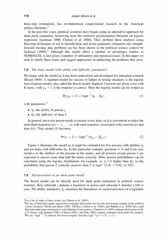
e0 and e1, as follows (see Figure 5):

Prðyi ¼ 1Þ ¼ e0 þ ð1 � e0 � e1Þlogit�1ðckðiÞðajðiÞ � bkðiÞÞÞ:

Within the Bayesian context, we allow the error rates, e0 and e1, to be estimated from data

by assigning them independent Uniform(0,0.1) prior distributions. (If the error rates were

much higher than 10%, we would not want to be fitting even an approximate logit model.)

4 Ideal point modeling for U.S. Supreme Court justices

We illustrate with an ideal point model fit to the voting records of U.S. Supreme Court

justices, using all the Court’s decisions from 1954 to 2000.7 Each vote i is associated with

a justice j(i) and a case k(i), with an outcome yi that equals 1 if a justice voted in the

conservative direction on a case and 0 if he or she voted in the liberal direction.8

Fig. 4 Plot of hypothetical probability distribution without and with outlier (in the upper left of the

right-hand plot). Realistically, outliers occur in political data, and we would not want our inferences

to be strongly affected by single outliers of the sort shown in the right-hand plot.

7The data were compiled by Harold J. Spaeth and can be downloaded from www.polisci.msu.edu/pljp.8The codings of ‘‘liberal’’ and ‘‘conservative’’ can sometimes be in error. As we shall discuss, the model with itsdiscrimination parameter allows us to handle and even identify possible miscodings of the directions of the votes(Jackman 2001).


http://www.polisci.msu.edu/pljp

As discussed in Section 2 of this paper, the data are modeled with a logistic regression,

with the probability of voting conservatively depending on the ‘‘ideal point’’ aj for each

justice, the ‘‘position’’ bk for each case, and a ‘‘discrimination parameter’’ ck for each case,

following the two-parameter logistic model (3):

Prðyi ¼ 1Þ ¼ logit�1ðckðiÞðajðiÞ � bkðiÞÞÞ: ð4Þ

The difference between aj and bk indicates the positions of the justices and the cases—

if a justice’s ideal point is near a case’s position, then the case could go either way, but if

the ideal point is far from the position, then the justice’s vote is highly predictable. The

discrimination parameter ck captures the importance of the positioning in determining the

justices’ votes: if ck ¼ 0, the votes on case k are purely random; if ck is very large (in

absolute value), then the relative positioning of justice and case wholly determine the

outcome. Changing the sign of gamma changes which justices are expected to vote yes and

which to vote no.

We fit the model using the Bayesian software WinBUGS (Spiegelhalter et al. 1999) as

called from R (Gelman 2003; R Development Core Team 2003). Two parallel chains

reached approximate convergence (using the adjusted parameterization described in

Section 2) after 15,000 iterations.

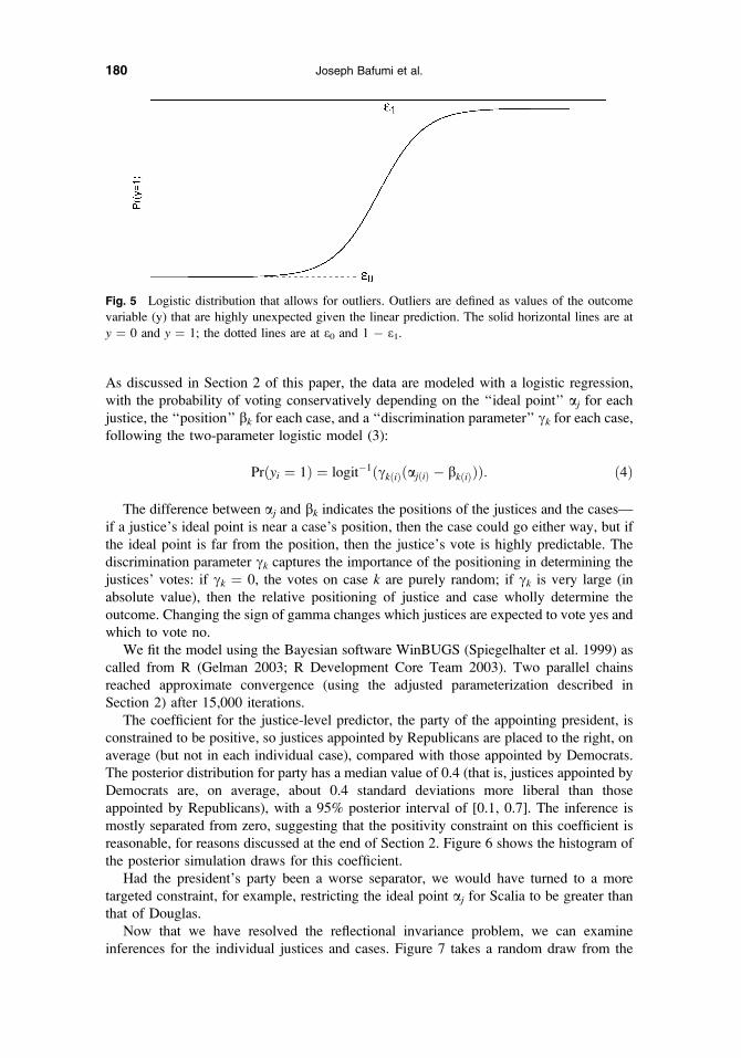
The coefficient for the justice-level predictor, the party of the appointing president, is

constrained to be positive, so justices appointed by Republicans are placed to the right, on

average (but not in each individual case), compared with those appointed by Democrats.

The posterior distribution for party has a median value of 0.4 (that is, justices appointed by

Democrats are, on average, about 0.4 standard deviations more liberal than those

appointed by Republicans), with a 95% posterior interval of [0.1, 0.7]. The inference is

mostly separated from zero, suggesting that the positivity constraint on this coefficient is

reasonable, for reasons discussed at the end of Section 2. Figure 6 shows the histogram of

the posterior simulation draws for this coefficient.

Had the president’s party been a worse separator, we would have turned to a more

targeted constraint, for example, restricting the ideal point aj for Scalia to be greater than

that of Douglas.

Now that we have resolved the reflectional invariance problem, we can examine

inferences for the individual justices and cases. Figure 7 takes a random draw from the

Fig. 5 Logistic distribution that allows for outliers. Outliers are defined as values of the outcome

variable (y) that are highly unexpected given the linear prediction. The solid horizontal lines are at

y ¼ 0 and y ¼ 1; the dotted lines are at e0 and 1 � e1.


posterior distribution and plots the positions bk of the cases, on top of the posterior median

estimates of the justices’ ideal points aj. Both cases and justices are plotted across court

terms. The positions of the cases appear stable over time, but there is a trend toward more

conservative justices.9 This is consistent with the widely accepted notion of a rightward-

shifting court.

In plotting the cases on the same scale as the justices, Figure 7 reveals, perhaps

surprisingly, that many of the cases are estimated to be outside the range of all nine justices

of the court. In fact, however, nearly 40% of the cases in our dataset were unanimous

decisions, and it makes sense that most of these would have extreme positions on one side

or another.

Figure 8 plots a random draw from the discrimination parameters’ posterior

distribution. Relatively few of the cases have negative discrimination parameters (less

than 5%). Since this is likely to be a sign of miscoding in the original data, it is a welcome

result. Negative discrimination parameters may also result from switching coalitions in

which conservative justices vote in what would a priori seems to be the liberal direction

while liberal justices vote in the conservative direction. Of the cases with negative median

discrimination parameter posterior distributions, about 25% are judicial power cases, 18%

are economic activity cases, and 10% each are federalism and interstate relations cases.

Switching coalitions or miscodes prove to be most likely with judicial power cases. The

higher the value of the discrimination parameter, the more likely the outcome of the case

depends on a left-right ideological construct. Of the discrimination posterior distribution

medians that exceed a value of 5, the plurality, 44%, are criminal procedure cases. Not

surprisingly, they seem to discriminate best between liberal and conservative justices.

Another 20% of these cases involve civil rights.

Fig. 6 Histogram of the coefficient of the president’s party predictor in the group-level regression

for the justice location parameters aj. Inference for the coefficient, which is restricted to be positive to

identify the model, is mostly separated from zero, indicating that that this constraint is a reasonable

(if not perfect) way to break the reflection invariance.

9As can be seen from the horizontal lines in Figure 7, our model constrains each justice to have an unchangingideology over time.


Such plots serve as a rough verification of model fit. They show results that make sense

given what we would expect about the Supreme Court. However, models designed to

generate ideal points, and item-response models more generally, can and should undergo

more rigorous tests of model fit. To this we turn next.

5 Assessing model fit

Statistical modelers typically spend little time rigorously judging model fit, even when

such checks can result in discoveries that greatly improve one’s model. For ideal point

estimates, one can test one aspect of model fit by checking the prediction errors, which can

be classically defined as10

ei ¼ 1 if (E(yi) . 0.5 and yi ¼ 0), or (E(yi) , 0.5 and yi ¼ 1)

0 otherwise.

n

It is useful to consider the excess error rate: the proportion of error beyond what would be

expected, in absolute value, given the model’s predicted values. First we need to

understand how to calculate what we would expect the error rate to be. If the model were

true, the probability of error, and thus the expected error rate, is simply the minimum of the

model’s prediction and 1 minus this prediction:

EðeiÞ ¼ minðlogit�1ðckðiÞðajðiÞ � bkðiÞÞÞ; 1 � logit�1ðckðiÞðajðiÞ � bkðiÞÞÞÞ:

The excess error can then be formalized as follows:

Excess errori ¼ ei � EðeiÞ:

1960 1970 1980 1990 2000

−5

05

Supreme Court Term

Ideo

logi

cal P

ositi

on

Fig. 7 A random draw from the posterior distribution of the positions bk of the cases (the dots on the

graph), and the posterior median estimates of the ideal points aj of the 29 justices (the lines), as

estimated using the Supreme Court model. Points on the ideal point line reflect cases for which that

justice is indifferent.

10These ei’s are ‘‘errors’’ rather than ‘‘residuals’’ because they are defined based on the parameter values a, b, c,not on point estimates a, b, c. With Bayesian inference, we can work directly with draws from the posteriordistribution of the parameters—as we illustrate in Figure 9—and thus do not need to use point estimates. Ourapproach has the advantage that the errors are independent in their posterior distribution and are thus moreconvenient to work with (see Gelman et al. 2000).


Individual-level errors are difficult to interpret usefully. However, averages of errors,

which offer 0 as a baseline or expectation, convey more meaningful information. Here we

shall investigate the excess error rate for each justice in our data. We plot the excess error

rate per justice across the justices’ ideal points. We plot the values from five separate

draws to capture the uncertainty in the posterior distributions. These are the realized error

rates (Gelman 2004). To provide a reference distribution for the model check, we generate

replicated y’s from our model and also plot their excess error rate per justice across the

justices’ ideal points.11 The excess errors computed from the replicated y’s show the range

of values that could be expected if our model were true.

Figure 9 shows five random draws of the realized excess error rates on the top row, with

corresponding draws from the reference distribution on the bottom row. The excess error

rate’s in the reference plots are generally low, implying that, with our sample sizes, the

error rate for each justice should be close to its expected value. The realized residuals show

less precision. In general, the ideal points of conservative justices can be estimated more

predictably than liberal justices. Particularly, the ideal points for justices 2 and 3 (Black

and Douglas) have high excess error rates. Justice Black has an error rate that is over 50%

higher than we would expect if our model were true. Justice Douglas has an error rate that

is over one-third higher than expected. Douglas’s ideal point is probably hard to estimate

because there is no one to anchor him to his left (Poole n.d.). Meanwhile, Black has been

shown to undergo significant shifts over time in his ideological ideal point even after

controlling for docket effects (Bafumi et al. 2002). Where model fit shows room for

improvement, one can revisit the specification of the original model.

The most noticeable pattern in the bottom row of graphs in Figure 9 is that the excess

error rates for justices 17, 14, and 15 (Jackson, Fortas, and Goldberg) appear likely to have

high absolute values in the replicated datasets. These potentially high errors arise because

1960 1970 1980 1990 2000

−5

05

1015

Supreme Court Term

Dis

crim

inat

ion

Fig. 8 A random draw from the posterior distribution of the discrimination parameters ck of the

cases plotted across Supreme Court terms. Dots represent individual cases. Values higher in absolute

value point to cases that better discriminate between liberal and conservative justices. Negative

discrimination parameters correspond to cases whose precoding is inconsistent with the ideological

ordering of justices estimated from the entire dataset.

11For each random draw of the vector of parameters (a, b, c), we generate a vector of replicated y’s by randomlydrawing each yi from a binomial distribution with n ¼ 1 and p ¼ logit�1(ck(i)(aj(i) � bk(i))).


−2

01

−0.6−0.4−0.20.00.20.40.6Avg

. Res

idu

als

Idea

l Poi

nt

Excess1

2

34

5 6

7

8

910 1112131415

1617 18

19

2021

22

23

2425

262

7

2829

−2

01

−0.6−0.4−0.20.00.20.40.6

Rep

licat

ion

s

Idea

l Poi

nt

Excess

12

34

5 67

8910 1112 13

1415

1617 1819

20

2122

23

24

25

26

27

2829

−2

01

−0.6−0.4−0.20.00.20.40.6Avg

. Res

idu

als

Idea

l Poi

ntExcess

1

2

34

5 6

7

8

910 11 1213

1415

1617

18

19

2021

22

23

24

2526

27

2829

−2

01

−0.6−0.4−0.20.00.20.40.6

Rep

licat

ion

s

Idea

l Poi

nt

Excess

12

34

567

89 1011 1213

14151617

1819

2021

2223

24

25

26

27

28 29

−2

01

−0.6−0.4−0.20.00.20.40.6Avg

. Res

idu

als

Idea

l Poi

nt

Excess

1

2

3

4

5 6

7

8

910 11 1213

1415

1617

18

19

2021

22

2324

2526

27

2829

−2

01

−0.6−0.4−0.20.00.20.40.6

Rep

licat

ion

s

Idea

l Poi

nt

Excess

12

34

567

89

1011 121314 15

1617

18

19

2021

2223

2425

262

728 29

−2

01

−0.6−0.4−0.20.00.20.40.6Avg

. Res

idu

als

Idea

l Poi

nt

Excess

1

3

4

56

7

8

910 11 1213

1415

16 17 18

19

20

21

22

2324

2526

27

2829

−2

01

−0.6−0.4−0.20.00.20.40.6

Rep

licat

ion

s

Idea

l Poi

nt

Excess

12

34

567

8910 11 12 13

1415

16 171819

2021

2223

2425

26

27

2829

−2

01

−0.6−0.4−0.20.00.20.40.6Avg

. Res

idu

als

Idea

l Poi

nt

Excess

1

2

34

56

7

8

910 111213

1415

16 17

18

19

2021

22

23

2425

262

72829

−2

01

−0.6−0.4−0.20.00.20.40.6

Rep

licat

ion

s

Idea

l Poi

nt

Excess

12

34

567

8

9101112 13

14 1516 17

1819

2021

2223

24

25

262

72829

184

our data provide little information on these justices,12 hence their ideal points are estimated

with less accuracy and there is more room for error in the prediction. However, as the top

row of Figure 9 shows, the largest data errors are for Justices Black and Douglas, as

discussed above.

One can also judge the overall fit of a discrete-data regression using calibration from

pooled predictions. A calibration plot allows us to compare the fitted (predicted) versus the

actual average values of y within bins. For example, one would begin by selecting the

number of bins to analyze; more bins allow for more fine-grained analyses. Then one

would isolate the fitted values for y that fall in each bin. For example, we can examine the

number of fitted values for 10 bins: 0–0.1, 0.1–0.2, . . . . Then we calculate the mean for

the fitted y’s that fall into each bin. Next, we calculate the mean of the corresponding

actual y’s. Plotted together, the means of the fitted versus actual y’s should fall on the 458

line. This is shown in the first column of Figure 10. The actual and fitted y’s show about

the same vote probability in each of the ten bins. We can also inspect a binned residual plot

(Gelman et al. 2003) by substracting the mean of the fitted y’s from the mean of the actual

y’s across each bin and plotting this new result across the fitted y’s. We expect no dis-

cernible pattern and residuals close to 0. This is shown in the second column of Figure 10.

Fig. 10 Calibration and binned residual plots with 10 bins for checking model fit. In a well-fitting

model, the mean of the binned actual y’s and the mean of the binned fitted y’s fall on the 458 angle, as

seen above. The differences between the two measures are almost all less than 1.5%.

Fig. 9 Plots of excess error rate in real and replicated values of the justices’ votes. Numbers label

justices as follows: 1 Harlan, 2 Black, 3 Douglas, 4 Stewart, 5 Marshall, 6 Brennan, 7 White, 8

Warren, 9 Clark, 10 Frankfurther, 11 Whittaker, 12 Burton, 13 Reed, 14 Fortas, 15 Goldberg, 16

Minton, 17 Jackson, 18 Burger, 19 Blackmun, 20 Powell, 21 Rehnquist, 22 Stevens, 23 O’Connor,

24 Scalia, 25 Kennedy, 26 Souter, 27 Thomas, 28 Ginsburg, 29 Breyer. For all plots, the average

excess error rate per justice is plotted across the justices’ ideal points. The replications show what we

would expect if our model were true. The realized residuals show room for model improvement.

‹

12Fortas and Goldberg served for only a few years each, and Jackson’s Court service ended shortly after the startof our dataset.


There is much further room for studying model fit, in particular by plotting the estimated

parameters bk and ck for groups of cases and exploring potential flaws in the logistic

regression model, which would possibly correspond to additional dimensions in the data.

6 Conclusion

Ideal point estimation has become common in political science research today. With the

increased use of this method, political methodologists have spent more time working to

improve the quality of these scores. This article investigates a series of practical issues that

arise with the estimation of ideal points and offers solutions that have not been commonly

applied to date. Problems include proper variance estimates, scale and translation

invariance, reflection invariance, and outliers. Resolutions to these issues come in the

form of Bayesian hierarchical modeling, linear transformations, informative regression

predictors, and explicit modeling for outliers. In addition, we explored new ways to usefully

display inferences and check model fit.

The procedures investigated above apply to unidimensional models. They do not account

for additional dimensions that explain votes or decisions beyond the left-right ideologi-

cal construct. However, the innovations could be generalized to such multidimensional

models. In fact, many could be generalized to Bayesian models of all sorts (for example,

transformations that aid in interpretation or convergence and model checking). Similar

issues arise in latent-class models and factor analysis (Loken 2004). Also, the substantive

model explored in Section 4 (to estimate the ideal points of Supreme Court justices) can be

developed much further. For example, it can be expanded to test propositions such as

shifting ideal points among justices over time (Martin and Quinn 2001, 2002a, 2002b). This

we leave to future work.

As Congress and judiciary scholarship continue to grow, the demand for high-quality

ideal point estimates will also grow. These scores are one of several resources that scholars

can use to understand the workings of government. Others include in-depth studies (Fenno

1978), legislator interviews (Lahav 2004), and a variety of scores that capture legislators’

underlying ideological ideal points without the complexity associated with NOMINATE

or Bayesian estimates such as content coding, special-interest group scores, or simple

tabulations (Bafumi et al. 2002). Growing research in each of these areas will benefit the

scholarship as a whole.

References

Bafumi, Joseph, Noah Kaplan, Nolan McCarty, Keith Poole, Andrew Gelman, and Charles Cameron. 2002.

‘‘Scaling the Supreme Court: A Comparison of Alternative Measures of the Justices’ Idealogical Preferences,

1953–2001.’’ Presented at the 2002 Annual Meeting of the Midwest Political Science Association, Chicago, IL.

Clinton, Joshua. 2001. ‘‘Legislators and their Constituencies: Representation in the 106th Congress.’’ Presented at

the 2001 Annual Meeting of the American Political Science Association, San Francisco, CA.

Clinton, Joshua, Simon Jackman, and Douglas Rivers. 2003. ‘‘The Statistical Analysis of Roll Call Data.’’

Technical Report: Political Methodology Working Papers.

Clinton, Joshua, Simon Jackman, and Douglas Rivers. 2004. ‘‘The Statistical Analysis of Roll Call Data.’’

American Political Science Review 98:355–370.

Fenno, Richard F. 1978. Home Style: House Members in Their Districts. Boston: Little, Brown.

Gelman, Andrew. 2003. Bugs.R: Functions for Calling Bugs from R. Available at http://www.stat.columbia.edu/

;gelman/bugsR.

Gelman, Andrew. 2004. ‘‘Exploratory Data Analysis for Complex Models (with Discussion).’’ Journal of

Computational and Graphical Statistics 13:755–779.

Gelman, Andrew, John S. Carlin, Hal S. Stern, and Donald B. Rubin. 2003. Bayesian Data Analysis. 2nd ed.

Boca Raton: Chapman and Hall.


http://www.stat.columbia.edu/~gelman/bugsR

http://www.stat.columbia.edu/~gelman/bugsR

Gelman, Andrew, and Donald B. Rubin. 1992. ‘‘Inference from Iterative Simulation using Multiple Sequences

with Discussion.’’ Statistical Science 7:457–511.

Gilks, Wally, R., Sylvia Richardson, and David J. Spiegelhalter, eds. 1996. Markov Chain Monte Carlo in

Practice. London: Chapman & Hall.

Jackman, Simon. 2000. ‘‘Estimation and Inference are Missing Data Problems: Unifying Social Science Statistics

via Bayesian Simulation.’’ Political Analysis 8:307–332.

Jackman, Simon. 2001. ‘‘Multidimensional Analysis of Roll Call Data via Bayesian Simulation: Identification,

Estimation, and Model Checking.’’ Political Analysis 9:227–241.

Lahav, Gallya. 2004. Immigration and Politics in the New Europe. Reinventing Borders. London: Cambridge

University Press.

Liu, Chuanahai. 2004. Robit Regression: A Simple Robust Alternative to Logistic and Probit Regression. In

Applied Bayesian Modeling and Casual Inference from an Incomplete-Data Perspective, ed. Andrew Gelman

and X. L. Meng. London: Wiley chapter 21.

Liu, Chuanhai, Donald B. Rubin, and Yingnian Wu. 1998. ‘‘Parameter Expansion to Accelerate EM: The PX-EM

Algorithm.’’ Biometrika 85:755–770.

Loken, Eric. 2004. Multimodality in Mixture Models and Factor Models. In Applied Bayesian Modeling and

Causal Inference from an Incomplete-Data Perspective, ed. Andrew Gelman and X. L. Meng, London: Wiley,

chap. 19.

Martin, Anderew D., and Kevin M. Quinn. 2001. ‘‘The Dimensions of Supreme Court Decision Making: Again

Revisiting The Judicial Mind.’’ Presented at the 2001 meeting of the Midwest Political Science Association.

Martin, Andrew D., and Kevin M. Quinn. 2002a. ‘‘Assessing Preference Change on the U.S. Supreme Court.’’

Presented at the University of Houston, March 15, 2002.

Martin, Andrew D., and Kevin M. Quinn. 2002b. ‘‘Dynamic Ideal Point Estimation via Markov Chain Monte

Carlo for the U.S. Supreme Court, 1953–1999.’’ Political Analysis 10:134–153.

Park, David. 2001. ‘‘Representation in the American States: The 100th Senate and Their Electorate.’’

Unpublished working paper.

Poole, Keith T. n.d. ‘‘Spatial Models of Parliamentary Voting.’’ Unpublished manuscript.

Poole, Keith T., and Howard Rosenthal. 1997. Congress: A Political-Economic History of Roll Call Voting.

New York: Oxford University Press.

Pregibon, D. 1982. ‘‘Resistant Fits for Some Commonly Used Logistic Models with Medical Applications.’’

Biometrics 38:485–498.

R Development Core Team. 2003. R: A Language and Environment for Statistical Computing. Vienna, Austria:

R. Foundation for Statistical Computing. Available at http://www.R-Project.org.

Rasch, George. 1980. Probabilistic Models for Some Intelligence and Attainment Tests. Chicago: University of

Chicago Press.

Rivers, Douglas. 2003. ‘‘Identification of Multidimensional Spatial Voting Models.’’ Technical Report: Political

Methodology Working Papers.

Spiegelhalter, David J., Andrew Thomas, and Nickey G. Best. 1999. WinBugs Version 1.4. Cambridge: MRC

Biostatistics Unit.


http://www.R-Project.org

practical issues in implementing and understanding ...gelman/research/published/171.pdf ·...

Documents