Practical heteroskedastic Gaussian process modeling forlarge simulation experiments

Mickael Binois∗ Robert B. Gramacy† Mike Ludkovski‡

Abstract

We present a unified view of likelihood based Gaussian progress regression for sim-ulation experiments exhibiting input-dependent noise. Replication plays an importantrole in that context, however previous methods leveraging replicates have either ig-nored the computational savings that come from such design, or have short-cut fulllikelihood-based inference to remain tractable. Starting with homoskedastic processes,we show how multiple applications of a well-known Woodbury identity facilitate infer-ence for all parameters under the likelihood (without approximation), bypassing thetypical full-data sized calculations. We then borrow a latent-variable idea from ma-chine learning to address heteroskedasticity, adapting it to work within the same thriftyinferential framework, thereby simultaneously leveraging the computational and statis-tical efficiency of designs with replication. The result is an inferential scheme that canbe characterized as single objective function, complete with closed form derivatives,for rapid library-based optimization. Illustrations are provided, including real-worldsimulation experiments from manufacturing and the management of epidemics.

Key words: stochastic kriging, input-dependent noise, Woodbury formula, replication

1 Introduction

Simulation-based experimentation has been commonplace in the physical and engineering

sciences for decades, and has been advancing rapidly in the social and biological sciences. In

both settings, supercomputer resources have dramatically expanded the size of experiments.

In the physical/engineering setting, larger experiments are desired to enhance precision and

to explore larger parameter spaces. In the social and biological sciences there is a third reason:

∗Corresponding author: The University of Chicago Booth School of Business, 5807 S. Woodlawn Ave.,Chicago IL, 60637; mbinois@chicagobooth.edu†Department of Statistics, Virginia Tech, Hutcheson Hall, 250 Drillfield Drive, Blacksburg, VA 24061‡Department of Statistics and Applied Probability, University of California Santa Barbara, 5520 South

Hall Santa Barbara, CA 93106-3110

1

arX

iv:1

611.

0590

2v2

[st

at.M

E]

13

Nov

201

7

stochasticity. Whereas in the physical sciences solvers are often deterministic, or if they

involve Monte Carlo then the rate of convergence is often known (Picheny and Ginsbourger,

2013), in the social and biological sciences simulations tend to involve randomly interacting

agents. In that setting, signal-to-noise ratios can vary dramatically across experiments and

for configuration (or input) spaces within experiments. We are motivated by two examples,

from inventory control (Hong and Nelson, 2006; Xie et al., 2012) and online management of

emerging epidemics (Hu and Ludkovski, 2017), which exhibit both features.

Modeling methodology for large simulation efforts with intrinsic stochasticity is lagging.

One attractive design tool is replication, i.e., repeated observations at identical inputs. Repli-

cation offers a glimpse at pure simulation variance, which is valuable for detecting a weak

signal in high noise settings. Replication also holds the potential for computational savings

through pre-averaging of repeated observations. It becomes doubly essential when the noise

level varies in the input space. Although there are many ways to embellish the classical GP

setup for heteroskedastic modeling, e.g., through choices of the covariance kernel, few ac-

knowledge computational considerations. In fact, many exacerbate the problem. A notable

exception is stochastic kriging (SK, Ankenman et al., 2010) which leverages replication for

thriftier computation in low signal-to-noise regimes, where it is crucial to distinguish intrinsic

stochasticity from extrinsic model uncertainty. However, SK has several drawbacks. Infer-

ence for unknowns is not based completely on the likelihood. It has the crutch of requiring

(a minimal amount of) replication at each design site, which limits its application. Finally,

the modeling and extrapolation of input-dependent noise is a secondary consideration, as

opposed to one which is fully integrated into the joint inference of all unknowns.

Our contributions address these limitations from both computational and methodological

perspectives. On the computational side, we expand upon a so-called Woodbury identity

to reduce computational complexity of inference and prediction under replication: from

the (log) likelihood of all parameters and its derivatives, to the classical kriging equations.

2

We are not the first to utilize the Woodbury “trick“ with GPs (see, e.g., Opsomer et al.,

1999; Banerjee et al., 2008; Ng and Yin, 2012), but we believe we are the first to realize its

full potential under replication in both homoskedastic and heteroskedastic modeling setups.

We provide proofs of new results, and alternate derivations leading to simpler results for

quantities first developed in previous papers, including for SK. For example, we establish—

as identities—results for the efficiency of estimators leveraging replicate-averaged quantities,

which previously only held in expectation and under fixed parameterization.

On the methodological end, we further depart from SK and borrow a heteroskedastic

modeling idea from the machine learning literature (Goldberg et al., 1998) by constructing

an apparatus to jointly infer a spatial field of simulation variances (a noise-field) along with

the mean-field GP. The structure of our proposed method is most similar to the one described

in Kersting et al. (2007) who turn a “hard expectation maximization (EM)” problem, with

expectation replacing the expensive Markov Chain Monte Carlo (MCMC) averaging over

latent variables, into a pure maximization problem. Here, we show how the Woodbury trick

provides two-fold computational and inferential savings with replicated designs: once for

conventional GP calculations arising as a subroutine in the wider heteroskedastic model,

and twice by reducing the number of latent variables used to described the noise field. We

go on to illustrate how we may obtain inference and prediction in the spirit of SK, but via

full likelihood-based inference and without requiring minimal replication at each design site.

A limitation of the Kersting et al. pure maximization approach is a lack of smoothness

in the estimated latents. We therefore propose to interject an explicit smoothing back into

the objective function being optimized. This smoother derives from a GP prior on the

latent (log) variance process, and allows one to explicitly model and optimize the spatial

correlation of the intrinsic stochasticity. It serves to integrate noise-field and mean-field

in contrast to the SK approach of separate empirical variance calculations on replicates,

followed by independent auxiliary smoothing for out-of-sample prediction. We implement

3

the smoothing in such a way that full derivatives are still available, for the latents as well

as the coupled GP hyperparameters, so that the whole inferential problem can be solved

by deploying an off-the-shelf library routine. Crucially, our smoothing mechanism does not

bias the predictor at the stationary point solving the likelihood equations, compared to an

un-smoothed alternative. Rather, it has an annealing effect on the likelihood, and makes the

solver easier to initialize, both accelerating its convergence.

The remainder of the paper is organized as follows. In Section 2 we review relevant GP

details, SK, and latent noise variables. Section 3 outlines the Woodbury trick for decompos-

ing the covariance when replication is present, with application to inference and prediction

schemes under the GP. Practical heteroskedastic modeling is introduced in Section 4, with

the Woodbury decomposition offering the double benefit of fewer latent variables and faster

matrix decompositions. An empirical comparison on a cascade of alternatives, on toy and

real data, is entertained in Section 5. We conclude with a brief discussion in Section 6.

2 GPs under replication and heteroskedasticity

Standard kriging builds a surrogate model of an unknown function f : Rd → R given a set of

noisy output observations Y = (y1, . . . , yN)> at design locations X = (x1, . . . ,xN)>. This is

achieved by putting a so-called Gaussian process (GP) prior on f , characterized by a mean

function and covariance function k : Rd × Rd → R. We follow the simplifying assumption

in the computer experiments literature in using a mean zero GP, which shifts all of the

modeling effort to the covariance structure. The covariance or kernel k is positive definite,

with parameterized families such as the Gaussian or Matern being typical choices.

Observation model is y(xi) = f(xi) + εi, εi ∼ N (0, r(xi)). In the typical homoskedastic

case r(x) = τ 2 is constant, but we anticipate heteroskedastic models as well. In this setup,

the modeling framework just described is equivalent to writing Y ∼ NN(0,KN +ΣN), where

4

KN is the N ×N matrix with ij coordinates k(xi,xj), and ΣN = Diag(r(x1), . . . , r(xN)) is

the noise matrix. Notice that xi is a d× 1 vector and the εi’s are i.i.d..

Given a form for k(·, ·), multivariate normal (MVN) conditional identities provide a

predictive distribution at site x: Y (x)|Y, which is Gaussian with parameters

µ(x) = E(Y (x)|Y) = k(x)>(KN + ΣN)−1Y, where k(x) = (k(x,x1), . . . , k(x,xN))>;

σ2(x) = Var(Y (x)|Y) = k(x,x) + r(x)− k(x)>(KN + ΣN)−1k(x).

The kernel k has hyperparameters that must be estimated. Among a variety of methods,

many are based on the likelihood, which is simply a MVN density. Most applications involve

stationary kernels, k(x,x′) = νc(x−x′;θ), i.e., KN = νCN , with ν being the process variance

and θ being additional hyperparameters of the correlation function c. After relabeling KN +

ΣN = ν(CN + ΛN), first order optimality conditions provide a plug-in estimator for the

common factor ν: ν = N−1Y>(CN + ΛN)−1Y. The log-likelihood conditional on ν is then:

logL = −N2

log(2π)− N

2log ν − 1

2log |CN + ΛN | −

N

2. (1)

Observe that we must decompose (e.g., via Cholesky) CN +ΛN potentially multiple times in

a maximization scheme, for inversion and determinant computations, which requires O(N3)

operations for the typical choices of c. This cubic computation severely limits the experiment

size, N , that can be modeled with GPs. Some work-arounds for large data include approxi-

mate strategies (e.g., Banerjee et al., 2008; Haaland and Qian, 2011; Kaufman et al., 2012;

Eidsvik et al., 2014; Gramacy and Apley, 2015) or a degree of tailoring to the simulation

mechanism or the input design (Plumlee, 2014; Nychka et al., 2015).

Replicates: When replication is present, some of the design sites are repeated. This

offers a potential computational advantage via switching from the full-N size of the data to

5

the unique-n number of unique design locations. To make this precise, we introduce a special

notation; note that our setting is fully generic and nests the standard setting by allowing

the number of replicates to vary site-to-site, or be absent altogether.

Let xi, 1 = i, . . . , n represent the n � N unique input locations, and y(j)i be the jth

out of ai ≥ 1 replicates, i.e., j = 1, . . . , ai, observed at xi, wheren∑i=1

ai = N . Then

let Y = (y1, . . . , yn)> collect averages of replicates, yi = 1ai

ai∑j=1

y(j)i . We now develop a

map from full KN ,ΣN matrices to their unique-n counterparts. Without loss of general-

ity, assume that the data are ordered so that X = (x1, . . . , x1, . . . xn)> where each input

is repeated ai times, and where Y is stacked with observations on the ai replicates in

the same order. With X composed in this way, we have X = UX, with U the N × n

block matrix U = Diag(1a1,1, . . . ,1an,1), where 1k,l is k × l matrix filled with ones. Sim-

ilarly, KN = UKnU>, where Kn = (k(xi, xj))1≤i,j,≤n while U>ΣNU = AnΣn where

Σn = Diag(r(x1), . . . , r(xn)) and An = Diag(a1, . . . , an). This decomposition is the ba-

sis for the Woodbury identities exploited in Section 3. Henceforth, we utilize this notation

with n and N subscripts highlighting the size of matrices and vectors.

2.1 Stochastic kriging

A hint for the potential gains available with replication, while addressing heteroskedasticity,

appears in Ankenman et al. (2010) who show that the unique-n predictive equations

µn(x) = kn(x)>(Kn + A−1n Σn)−1Y where kn(x) = (k(x, x1), . . . , k(x, xn))>,

σ2n(x) = k(x,x) + r(x)− kn(x)>(Kn + A−1

n Σn)−1kn(x)

are unbiased and minimize mean-squared prediction error. This result implies that one can

handle N � n points in O(n3) time. A snag is that one can rarely presume to know the

6

variance function r(x). Ankenman et al., however show that with a sensible estimate

Σn = Diag(σ21, . . . , σ

2n), where σ2

i =1

ai − 1

ai∑j=1

(y(j)i − yi)2, (2)

in place of Σn the resulting µn(x) is still unbiased with ai � 1 (they recommend ai ≥ 10).

The predictive variance σ2n still requires an r(x), for which no observations are directly

available for estimation. One could specify r(x) = 0 and be satisfied with an estimate of

extrinsic variance, i.e., filtering heterogeneous noise (Roustant et al., 2012), however that

would preclude any applications requiring full uncertainty quantification. Alternatively,

Ankenman et al., proposed a second, separately estimated, (no-noise) GP prior for r trained

on the (xi, σ2i ) pairs to obtain a prediction for r(x) at new x locations.

Although this approach has much to recommend it, there are several notable shortcom-

ings. One is the difference of treatment between hyperparameters. The noise variances are

obtained from the empirical variance, while any other parameter, such as lengthscales θ for

k(·, ·), are inferred based on the pre-averaged log-likelihood (requiring O(n3) for evaluation):

log L := −n2

log(2π)− 1

2log |Kn + A−1

n Σn| −1

2Y>(Kn + A−1

n Σn)−1Y. (3)

While logical and thrifty, this choice of Σn leads to the requirement of a minimal number of

replicates, ai > 1 for all i, meaning that incorporating even a single observation without a

second replicate requires a new method (lest such valuable observation(s) be dropped from

the analysis). Finally, the separate modeling of the mean-field f(·) and its variance r(·) is

inefficient. Ideally, a likelihood would be developed for all unknowns jointly.

2.2 Latent variable process

Goldberg et al. (1998) were the first to propose a joint model for f and r, coupling a GP

7

on the mean with GP on latent log variance (to ensure positivity) variables. Although ideal

from a modeling perspective, and not requiring replicated data, inference for the unknowns

involved a cumbersome MCMC. Since each MCMC iteration involves iterating over each of

O(N) parameters, with acceptance criteria requiring O(N3) calculation, the method was

effectively O(TN4) to obtain T samples, a severely limiting cost.

Several groups of authors subsequently introduced thriftier alternatives in a similar spirit,

essentially replacing MCMC with maximization (Kersting et al., 2007; Quadrianto et al.,

2009; Lazaro-Gredilla and Titsias, 2011), but the overall computational complexity of each

iteration of search remained the same. An exception is the technique of Boukouvalas and

Cornford (2009) who expanded on the EM-inspired method of Kersting et al. (2007) to

exploit computational savings that comes from replication in the design. However that

framework has two drawbacks. One is that their mechanism for leveraging of replicates

unnecessarily, as we show, approximates predictive and inferential quantities compared to

full data analogues. Another is that, although the method is inspired by EM, the latent

log variances are maximized rather than averaged over, yielding a solution which is not a

smooth realization from a GP. Quadrianto et al. (2009) addressed that lack of smoothness

by introducing a penalization in the likelihood, but required a much harder optimization.

In what follows we ultimately borrow the modeling apparatus of Goldberg et al. and the

EM-inspired method of Kersting et al. and Quadrianto et al., but there are two important

and novel ingredients that are crucial to the adhesive binding them together. We show that

the Woodbury trick, when fully developed below, facilitates massive computational savings

when there is large-scale replication, achieving the same computational order as Boukouvalas

and Cornford and SK but without approximation. We then introduce a smoothing step that

achieves an EM-style averaging over latent variance, yet the overall method remains in a pure

maximizing framework requiring no simulation or otherwise numerical integration. Our goal

is to show that it is possible to get the best of all worlds: fully likelihood-based smoothed and

8

joint inference of the latent variances alongside the mean-field (mimicking Goldberg et al.

but with the O(n3) computational demands of SK). The only downside is that our point

estimates do not convey the same full posterior uncertainty as an MCMC would.

3 Fast GP inference and prediction under replication

We exploit the structure of replication in design for GPs with extensive use of two well-known

formulas, together comprising the Woodbury identity (e.g., Harville, 1997):

(D + UBV)−1 = D−1 −D−1U(B−1 + VD−1U)−1VD−1; (4)

|D + UBV| = |B−1 + VD−1U| × |B| × |D|, (5)

where D and B are invertible matrices of size N×N and n×n respectively, and U and V> are

of size N × n. In our context of GP prediction and inference, under the generic covariance

parameterization KN + ΣN = ν(CN + ΛN), we take the matrix D = ΣN = νΛN in (4)

as diagonal, e.g., νΛN = τ 2IN , and V = U>. Moreover, ΣN shares the low dimensional

structure, U>ΣNU = AnΣn = νAnΛn, and note that U>U = An. In combination, these

observations allow efficient computation of the inverse and determinant of (KN + ΣN). In

fact, there is no need to ever build the full-N matrices.

Lemma 3.1. We have the following full-N to unique-n identities for the GP prediction

equations, conditional on hyperparameters.

kN(x)>(KN + ΣN)−1Y = cn(x)>(Cn + ΛnA−1n )−1Y; (6)

kN(x)>(KN + ΣN)−1kN(x) = νcn(x)>(Cn + ΛnA−1n )−1cn(x). (7)

Eq. (6) establishes that the GP predictive mean, calculated on the average responses at

9

replicates and with covariances calculated only at the unique design sites, is indeed identical

to the original predictive equations built by overlooking the structure of replication. Eq. (7)

reveals the same result for the predictive variance. A proof of this lemma is in Appendix

A.1. These identities support common practice, especially in the case of the predictive

mean, of only utilizing the n observations in Y for prediction. Ankenman et al. (2010), for

example, show that this unique-n shortcut, applied via SK with Λn = ν−1Σn is the best

linear unbiased predictor (BLUP), after conditioning on the hyperparameters in the system.

This is simply a consequence of the unique-n predictive equations being identical to their

full-N counterpart, inheriting BLUP and any other properties.

Although aspects of the results above have been known for some time, if perhaps not

directly connected to the Woodbury formula, they were not (to our knowledge) known to

extend to the full likelihood. The lemma below establishes that indeed they do.

Lemma 3.2. Let Υn := Cn + A−1n Λn. Then we have the following unique-n identity for the

full-N expression for the conditional log likelihood, logL in Eq. (1).

logL = Const− N

2log νN −

1

2

n∑i=1

[(ai − 1) log λi + log ai]−1

2log |Υn|, (8)

where νN := N−1(Y>Λ−1

N Y − Y>AnΛ−1n Y + Y>Υ−1

n Y). (9)

The proof of the lemma is based on the following key computations:

Y>(CN + ΛN)−1Y = Y>Λ−1N Y − Y>AnΛ

−1n Y + Y>(Cn + A−1

n Λn)−1Y; (10)

log |CN + ΛN | = log |Cn + A−1n Λn|+

n∑i=1

[(ai − 1) log λi + log ai] . (11)

Assuming the n× n matrices have already been decomposed, at O(n3) cost, the extra com-

putational complexity is O(N + n) for the right-hand-side of (10) and O(n) for the right-

hand-side of (11), respectively. Both are negligible compared to O(n3).

10

It is instructive to compare (8–9) to the pre-averaged log likelihood (3) used by SK. In

particular, observe that the expression in (9) is different to the one that would be obtained by

estimating ν with unique-n calculations based on Y, which would give νn = n−1Y>Υ−1n Y,

an O(n2) calculation assuming pre-decomposed matrices. However, our full data calculation

via Y above gives νN = N−1(Y>Λ−1N Y − Y>AnΛ

−1n Y + nνn). The extra term in front of

νn is an important correction for the variance at replicates:

N−1(Y>Λ−1N Y − YAnΛ

−1n Y) = N−1

n∑i=1

aiλis2i , (12)

where s2i = 1

ai

∑aij=1(y

(j)i − yi)2, i.e., the bias un-adjusted estimate of Var(Y (xi)) based on

{y(j)i }

aij=1. Therefore, observe that as the ai get large, Eq. (12) converges toN−1

n∑i=1

aiλiVar(Y (xi)).

Note that computing (12) is in O(N + n2) with pre-decomposed matrices.

Finally, we provide the derivative of the unique-n log likelihood to aid in numerical

optimization, revealing a computational complexity in O(N + n3), or essentially O(n3):

∂ logL

∂·=N

2

∂(Y>Λ−1

N Y − YAnΛ−1n Y + nνn

)∂·

× (NνN)−1

− 1

2

n∑i=1

[(ai − 1)

∂ log λi∂·

]− 1

2tr

(Υ−1n

∂Υn

∂·

). (13)

The calculations above are presented generically so that they can be applied both in ho-

moskedastic and heteroskedastic settings. In a homoskedastic setting, recall that we may

take λi := λ = τ 2/ν, and no further modifications are necessary provided that we choose

a form for the covariance structure, generating Cn above, which can be differentiated in

closed form. In the heteroskedastic case, described in detail below, we propose a scheme for

estimating the latent λi value at the ith unique design location xi. Appendix A.2 provides an

empirical illustration of the computational savings that comes from utilizing these identities

in a homoskedastic context, and in the presence a modest degree of replication(3).

11

4 Practical heteroskedastic modeling

Heteroskedastic GP modeling involves learning the diagonal matrix ΛN (or its unique-n

counterpart Λn), allowing the λi values to exhibit heterogeneity, i.e., not all λi = τ 2/ν as in

the homoskedastic case. Care is required when performing inference for such a high dimen-

sional parameter. The strategy of Goldberg et al. (1998) involves applying regularization

in the form of a prior that enforces positivity and encourages a smooth evolution over the

input space. Inference is performed by integrating over the posterior of these latent values

with MCMC. This is a monumental task when N is large, primarily because mixing of the

latents is poor. We show that it is possible to have far fewer latent variables via Λn (recall

that U>ΛNU = AnΛn) when replication is present, via the Woodbury identities above, and

to achieve the effect of integration by maximizing a criterion involving smoothed quantities.

4.1 A new latent process formulation

A straightforward approach to learning Λn comes by maximizing the log likelihood (8).

As we show later in Figure 1 (top), this results in over-fit. As in many high-dimensional

settings, it helps to regularize. Toward that end Goldberg et al. suggest a GP prior for log λ.

This constrains the log Λn to follow a MVN law, but otherwise they are free to take on any

values. In particular, if the MVN acknowledges that our glimpse at the noise process, via the

observed (x, y)-values, is itself noisy, then the λis that come out, as may be obtained from a

local maximum of the resulting penalized likelihood (i.e., the joint posterior for mean-field

and noise processes), may not be smooth. Guaranteeing smoothed values via maximizing,

as an alternative to more expensive numerical integration, requires an explicit smoothing

maneuver in the “objective” used to solve for latents and hyperparameters.

Toward that end we re-cast the λ1, . . . , λn of Λn as derived quantities obtained via the

predictive mean of a regularizing GP on new latent variables δ1, . . . , δn, stored in diagonal

12

∆n for ease of manipulation. That is

log Λn = C(g)(C(g) + gA−1n )−1∆n =: C(g)Υ

−1(g)∆n, (14)

where C(g) generically denotes the correlation structure of this noise process, whose nugget

is g, and ∆n ∼ Nn(0, ν(g)(C(g) + gA−1n )). The appearance of the replication counts An

in Υ(g) = (C(g) + gA−1n ) is matching the structure of Υn in Section 3; see Lemma 3.2 or

Eq. (10). Thus the right-hand-side of (14) can be viewed as a smoother of the latent δi’s,

carried out in analogue to the GP equations for the mean-field. This setup guarantees that

every ∆n, e.g., as considered by a numerical solver maximizing a likelihood, leads to smooth

and positive variances Λn. Although any smoother could be used to convert latent ∆n into

Λn, a GP mimics the choice of post-hoc smoother in SK. The difference here is that the

inferential stage acknowledges a desire for smoothed predictions too.

Choosing a GP smoother has important implications for the stationary point of the com-

posite likelihood developed in Section 4.2 below, positioning smoothing as a computational

device that facilitates automatic initialization of the solver and an annealing of the objective

for improved numerical stability. The parameter g governs the degree of smoothing: when

g = 0 we have log Λn = ∆n, i.e., no smoothing; alternatively if C(g) = In and ∆n = In,

then log Λn = (g + 1)−1In and we recover the homoskedastic setup of Section 1 with noise

variance τ 2 = νN exp(1/(g + 1)).

To learn appropriate latent ∆n values (leaving details for other hyperparameters to Sec-

tion 4.2), we take advantage of a simple chain rule for the log-likelihood (13).

∂ logL

∂∆n

=∂Λn

∂∆n

∂ logL

∂Λn

= ΛnC(g)Υ−1(g)

∂ logL

∂Λn

, (15)

where∂ logL

∂λi=N

2×

ais2i

λ2i+

(Υ−1n Y)2iai

νN− ai − 1

2λi− 1

2ai(Υn)−1

i,i . (16)

13

With S = Diag(s21, . . . , s

2n), we may summarize (16) in a more convenient vectorized form as

∂ logL

∂Λn

=1

2

AnSΛ−2n + A−1

n Diag(Υ−1n Y)2

νN− An − In

2Λ−1n −

1

2A−1n Diag(Υ−1

n ). (17)

Recall that s2i = 1

ai

∑aij=1(y

(j)i − yj)2. Therefore, an interpretation of (16) is as extension

of the SK estimate σ2i at xi. In contrast with SK, observe that the GP smoothing is precisely

what facilitates implementation for small numbers of replicates, even ai = 1, in which case

even though s2i = 0, yi still contributes to the local variance estimates via the rest of Eq. (16).

Moreover, that smoothing comes nonparametrically via all latent δi variance variables. In

particular, note that (16) is not constant in δi; in fact it depends on all of ∆n via Eq. (14).

Remark 4.1. Smoothing may be entertained on other quantities, e.g., ΛnνN = C(g)Υ−1(g)Σ

2

n

(presuming ai > 1), resulting in smoothed moment-based variance estimates in the style of

SK, as advocated by in Kaminski (2015) and Wang and Chen (2016). There may similarly

be scope for bypassing a latent GP noise process with the so-called SiNK predictor (Lee and

Owen, 2015) by taking log Λn = ρ(X)−1C(g)Υ−1(g)∆n with ρ(x) =

√ν(g)c(g)(x)>Υ−1

(g)c(g)(x).

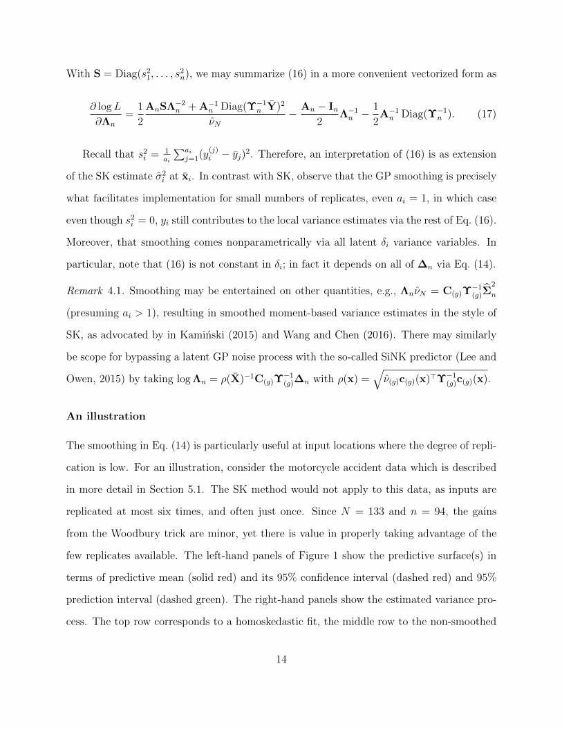
An illustration

The smoothing in Eq. (14) is particularly useful at input locations where the degree of repli-

cation is low. For an illustration, consider the motorcycle accident data which is described

in more detail in Section 5.1. The SK method would not apply to this data, as inputs are

replicated at most six times, and often just once. Since N = 133 and n = 94, the gains

from the Woodbury trick are minor, yet there is value in properly taking advantage of the

few replicates available. The left-hand panels of Figure 1 show the predictive surface(s) in

terms of predictive mean (solid red) and its 95% confidence interval (dashed red) and 95%

prediction interval (dashed green). The right-hand panels show the estimated variance pro-

cess. The top row corresponds to a homoskedastic fit, the middle row to the non-smoothed

14

heteroskedastic case, whereas the bottom row is based on (14). Aesthetically, the bottom

●●●●● ●●●●●●●●●●●●● ●●●

●●●●●●

●

●●

●●

●

●●

●●

●●

●

●

●

●

●

●

●

●

●

●

●

●●●●

●

●

●

●

●●●

●

●●

●●●

●

●

●

●

●●

●

●

●

●

●

●

●

●

●

●

●●●

●

●●

●

●

●

●

●●●

●

●

●

●

●

●

●

●●

●

●

●

●●●

●●

●

●

●

●

●

●

●●

● ●

●

●●

●

●

●

●

●

●

●

10 20 30 40 50

−15

0−

100

−50

050

100

time

acce

lera

tion ●●●●● ●●● ●●●●●●●●

● ●●●

●

●

●

●●●

●●

●

●●

●

●

●

●

●●●

●

●●

● ●●

●

●

●

●●

●

●

●●

●●

●

●●

●

●

●

●

●

●●

●

●

●

●

●

●

●

●

●

●●

●

●

●

●

●

●

●●

● ●

●

●

●

●

●

●●

●

Predictive surface (homoskedastic GP)

0 10 20 30 40 50 60

050

010

0015

0020

0025

00

time

σ2

Estimated constant variance

●●

●

●

●

●

●

●

●

●

●

●

● ●●

●

●

●

●

●

●

●

●

●

● ● ●

●●●●● ●●●●●●●●●●●●● ●●●

●●●●●●

●

●●

●●

●

●●

●●

●●

●

●

●

●

●

●

●

●

●

●

●

●●●●

●

●

●

●

●●●

●

●●

●●●

●

●

●

●

●●

●

●

●

●

●

●

●

●

●

●

●●●

●

●●

●

●

●

●

●●●

●

●

●

●

●

●

●

●●

●

●

●

●●●

●●

●

●

●

●

●

●

●●

● ●

●

●●

●

●

●

●

●

●

●

10 20 30 40 50

−15

0−

100

−50

050

100

time

acce

lera

tion ●●●●● ●●● ●●●●●●●●

● ●●●

●

●

●

●●●

●●

●

●●

●

●

●

●

●●●

●

●●

● ●●

●

●

●

●●

●

●

●●

●●

●

●●

●

●

●

●

●

●●

●

●

●

●

●

●

●

●

●

●●

●

●

●

●

●

●

●●

● ●

●

●

●

●

●

●●

●

Predictive surface (unsmoothed variance)

0 10 20 30 40 50 60

050

010

0015

0020

0025

00

time

σ2

Variance process (unsmoothed)

●●

●

●

●

●

●

●

●

●

●

●

● ●●

●

●

●

●

●

●

●

●

●

● ● ●

●●●●● ●●●●●●●●●●●●● ●●●

●●●●●●

●

●●

●●

●

●●

●●

●●

●

●

●

●

●

●

●

●

●

●

●

●●●●

●

●

●

●

●●●

●

●●

●●●

●

●

●

●

●●

●

●

●

●

●

●

●

●

●

●

●●●

●

●●

●

●

●

●

●●●

●

●

●

●

●

●

●

●●

●

●

●

●●●

●●

●

●

●

●

●

●

●●

● ●

●

●●

●

●

●

●

●

●

●

10 20 30 40 50

−15

0−

100

−50

050

100

time

acce

lera

tion ●●●●● ●●● ●●●●●●●●

● ●●●

●

●

●

●●●

●●

●

●●

●

●

●

●

●●●

●

●●

● ●●

●

●

●

●●

●

●

●●

●●

●

●●

●

●

●

●

●

●●

●

●

●

●

●

●

●

●

●

●●

●

●

●

●

●

●

●●

● ●

●

●

●

●

●

●●

●

Predictive surface (smoothed variance)

0 10 20 30 40 50 60

050

010

0015

0020

0025

00

time

σ2

Variance process (smoothed)

●●

●

●

●

●

●

●

●

●

●

●

● ●●

●

●

●

●

●

●

●

●

●

● ● ●

Figure 1: Motorcycle example for constant noise (top), with (bottom) and without (center)smoothing the λi values. Left: mean surface as a solid red line, with 95% confidence andprediction intervals in red dashed and green dotted lines, respectively. Open circles areactual data points; averaged observations yi (for inputs with ai > 1) are filled. Right: meansof the variance surface as red lines, empirical variance σ2

i at replicates as green points.

(smoothed variances) look better than the middle (un-smoothed) alternative. A more quan-

titative comparison, including alternatives from the literature, is provided in Section 5.1.

15

4.2 Simultaneous optimization of hyperparameters and latents

Smoothing (14) is key to sensible evolution of the noise process over the input space, but

perhaps the most important feature of our framework is how it lends itself to direct and

tractable inference via likelihood, without auxiliary calculation or simulation. Computational

complexity is linked to the degree of replication—O(n3) is much better than O(N3) if N �

n—however we remind the reader that no minimal degree of replication is required.

The full set of hyperparameters are determined by the correlation structure(s) of the

two GPs, as well as the latent ∆n. We denote by θ the lengthscales of the mean-field GP,

generating the n × n matrix Cn. Similarly, we use φ for the lengthscales in C(g), with the

degree of smoothing (14) determined by g. Inference requires choosing only values of these

parameters, {θ,φ,∆n, g}, because conditional on those, the scales ν and νg of both processes

have plug-in MLEs: νN in Eq. (9) and analogously ν(g) = n−1∆>nΥ−1(g)∆n. Therefore plugging

in νN and ν(g) yields the following concentrated joint log likelihood log L:

log L = − N

2log νN −

1

2

n∑i=1

[(ai − 1) log λi + log ai]−1

2log |Υn|

− n

2log ν(g) −

1

2log |Υ(g)|+ Const, (18)

where the top line above is the mean-field component, identical to (8), and the bottom one

is the analog for the latent variance process, all up to an additive constant.

Although seemingly close to the penalization used in Quadrianto et al. (2009), a key

difference here lies in the use of g, analogous to a homogeneous noise on the variance process.

Smoothing, via g, has an annealing effect on the optimization objective and, as Lemma 4.1

establishes, can have no adverse effect on the final solution. Our own preliminary empirical

work (not shown) echoes results of Lazaro-Gredilla and Titsias (2011) who demonstrate the

value of smoothing in this context as a guard against overfit.

16

Lemma 4.1. The objective log L in Eq. (18) is maximized when ∆n = log Λn and g = 0.

The proof is left in Appendix B.1, however some discussion may be beneficial. This result

says that smoothing (14) is redundant under the GP prior for ∆n: you’ll get a smooth answer

anyway, if you find the global maximum. If we initialize ∆n at a non-smooth setting, say via

an empirical estimate of variance derived from residual sums of squares from an initial GP

fit, an (initially) non-zero g-value will compensate and automatically generate a spatially

smooth Λn. As the solver progresses we can signal convergence—to a smoothed ∆n—if g

is (numerically) zero. Or, if on a tight computational budget, we can stop the solver early,

and rely on log Λn values being smooth, but close to their ∆n counterparts.

Inference for all unknowns may be carried out by a Newton-like scheme since the gradient

of (18) is available in closed form. Its components may be derived generically through

Eqs. (13–15), i.e., without separating out by hyperparameter, however we detail them below

for convenience. For each component θk of the mean-field lengthscale θ defining Cn, we have

∂ log L

∂θk=

1

2νNY>Υ−1

n

∂Cn

∂θkΥ−1n Y − 1

2tr

(Υ−1n

∂Cn

∂θk

). (19)

The rest of the components of the gradient depend on the derivative of the smoothed Λn,

i.e., ∂L∂Λn

in (17). For the latent variance parameters δi in ∆n, we have

∂ log L

∂∆n

= −Υ−1

(g)∆n

ν(g)

+ C(g)Υ−1(g)Λn ×

∂L

∂Λn

. (20)

For each component φk of the lengthscale of the noise process, φ, we have

∂ log L

∂φk=

[∂C(g)

∂φk−C(g)Υ

−1(g)

∂C(g)

∂φk

]Υ−1

(g)∆nΛn ×∂L

∂Λn

(21)

+1

2ν(g)

∆>nΥ−1(g)

∂C(g)

∂φkΥ−1

(g)∆n − tr

(Υ−1

(g)

∂C(g)

∂φk

).

17

And finally, for the noise-smoothing nugget parameter g we have

∂ log L

∂g= −C(g)Υ

−1(g)A

−1n Υ−1

(g)∆nΛn ×∂L

∂Λn

(22)

+1

2ν(g)

∆>nΥ−1(g)A

−1n Υ−1

(g)∆n − tr(A−1n Υ−1

(g)

).

4.3 Implementation details

Our implementation is in R (Core Team, 2014), available in the package hetGP Binois and

Gramacy (2017), essentially consists of feeding an objective, i.e., a coding of the joint log-

likelihood (18), and its gradient (19–22), into the optim library with method="lbfgsb". A

demonstration of the library, using the motorcycle data from Sections 4.1 & 5.1, is provided

in Appendix B.2. The implementation is lean on storage and avoids slow for loops in R. In

particular vectors, not matrices, are used to store diagonals like ∆n, An, Λn, etc. Traces of

non-diagonal matrices are calculated via compiled C++ loops, as are a few other calculations

that would otherwise have been cumbersome in R. We have found that a thoughtful initial-

ization of parameters, and in some cases a sensible restriction of their values (i.e., somewhat

limiting the parameter space), results in a faster and more reliable convergence on a tight

computing budget. E.g., no restarts are required.

Specifically, we find it useful to deploy a priming stage, wherein a single homoskedas-

tic GP (with the Woodbury trick) is fit to the data, in order to set initial values for

the latent variables and their GP hyperparameterization. Initial δi’s are derived from

the logarithm of residual sums of squares calculations on the fitted values obtained from

the homoskedastic GP, whose estimated lengthscales determine the initial θ and φ values,

δ0i = log

(1/ai

∑aij=1(µ(xi)− y(j)

i )2)

. An initial value for g is obtained via a separate, inde-

pendent homoskedastic GP fit to the resulting collection of ∆n, which may also be utilized

to refine the starting φ values. Our software includes the option of restricting the search

18

for lengthscales to values satisfying φ ≥ θ, taken component-wise. This has the effect of

forcing the noise process to evolve more slowly in space than the mean-field process does.

A thrifty approximate solution that avoids deploying a solver handling constraints involves

lower-bounding φ based on values of θ obtained from the initial homogeneous fit. We include

a further option restricting φ = kθ where the scalar k ≥ 1 is inferred in lieu of φ directly,

which is beneficial in higher dimensions.

Latent variable estimates returned by the optimizer can provide a good indication of the

nature of convergence. Any δj at the boundary of the lbfgsb search region either indicates

that the bounding box provided is too narrow, the initialization is poor, or that g needs to

be larger because the Λn values are being under-smoothed. Although we have iteratively

re-engineered our “automatic default” initializations and other settings of the software to

mitigate such issues, we find that in fact such adjustments usually have small impact on the

overall performance of the method. Numerical experiments backing the proposed initializa-

tion scheme are given in Appendix B.3.

After the solver has converged we conclude the procedure with comparison of the un-

penalized log-likelihood, i.e., the top part of Eq. (18), to one obtained from an optimized

homoskedastic fit. The latter may be higher if the optimization process was unsuccessful,

however typically the explanation is that there was not enough data to justify an input-

dependent noise structure. In that case we return the superior homoskedastic fit.

Remark 4.2. It is worth noting that working directly with latent variances Λn, rather than log

variances log Λn, might be appropriate if it is unreasonable to model the variance evolution

multiplicatively. The expressions provided above (19–22) simplify somewhat compared to

our favored logged version. However, a zero-mean GP prior on the (un-exponentiated) Λn

could yield negative predictions, necessitating thresholding. We suggest augmenting with a

non-zero constant mean term, i.e., µ(g) = 1>Υ−1(g)∆n

(1>Υ−1

(g)1)−1

as a potential means of

reducing the amount of thresholding required.

19

5 Empirical comparison

In what follows we consider three examples, starting with a simple expository one from

the literature, followed by two challenging “real data” computer model applications from

inventory optimization and epidemiology.

5.1 Benchmark data

One of the classical examples illustrating heteroskedasticity is the motorcycle accident data.

It consists of N = 133 accelerations with respect to time in simulated crashes, n = 94 of

which are measured at unique time inputs. Hence, this is a somewhat unfavorable example

as far as computational advantage goes (via Woodbury), however we note that a method like

SK would clearly not apply. Figure 1 provides a visualization of our performance on this data.

For the experimental work reported below we use the heteroskedastic fit from the bottom

row of that figure, corresponding to smoothed (log) latent variance parameters under full

MLE inference for all unknowns, denoted WHGP. See Appendix B.2 for an implementation

via mleHetGP in our hetGP library. We also include a homoskedastic GP comparator via our

Woodbury computational enhancements, using mleHomGP, abbreviated WGP.

Table 1 summarizes our results alongside ones of other methods in the literature, as ex-

tracted from Lazaro-Gredilla and Titsias (2011): another homoskedastic GP without Wood-

bury (labeled GP), a MAP alternative to the Goldberg et al. (1998) heteroskedastic GP

(labeled MAPHGP) from Kersting et al. (2007); Quadrianto et al. (2009) and a variational

alternative (VHGP) from Lazaro-Gredilla and Titsias (2011). The experiment involves 300

random (90%, 10%) partitions into training and testing data, with performance on the test-

ing data averaged over all partitions. Although we generally prefer a Matern correlation

structure, we used a Gaussian kernel for this comparison in order to remain consistent with

the other comparators. The metrics used, which are derived from the references above to

20

WGP WHGP GP (?) MAPHGP (?) VHGP (?)NMSE 0.28 ± 0.21 0.28 ± 0.21 0.26 ± 0.18 0.26 ± 0.17 0.26 ± 0.17NLPD 4.59 ± 0.25 4.26 ± 0.31 4.59 ± 0.22 4.32 ± 0.60 4.32 ± 0.30

Table 1: Average Normalized MSE and Negative Log-Probability Density (NLPD) ±1 sd onthe motorcycle data over 300 runs for our methods (WGP and WHGP) compared to those(?) reported in Lazaro-Gredilla and Titsias (2011). Lower numbers are better.

avoid duplicating the efforts in those studies, are Normalized Mean Squared Error (NMSE)

and Negative Log-Probability Density (NLPD), the latter being, up to a constant, the nega-

tive of the proper scoring rule we prefer in our next example. For details see Lazaro-Gredilla

and Titsias (2011). The take-away message from the table is that our proposed methods are

comparable, in terms of accuracy, to these comparators. We report that our WHGP method

took less than one second to perform 100 optim iterations.

5.2 Assemble to order

Here we consider the so-called “assemble-to-order” (ATO) problem first introduced by Hong

and Nelson (2006). At its heart it is an optimization (or reinforcement learning) problem,

however here we simply treat it as a response surface to be learned. Although the signal-

to-noise ratio is relatively high, ATO simulations are known to be heteroskedastic, e.g., as

illustrated by the documentation for the MATLAB library we utilized for the simulations

(Xie et al., 2012). The problem centers around inventory management for a company that

manufactures m products. Products are built from base parts, called items, some of which

are “key” in that the product cannot be built without them. If a request comes in for a

product which is missing one or more key items, a replenishment order is executed, and is

filled after a random period. Holding items in inventory is expensive, so there is a balance to

be struck between the cost of maintaining inventory, and revenue which can only be realized

if the inventory is sufficient to fulfill demand for products.

The inventory costs, product revenue, makeup of products (their items), product demand

21

stream and distribution of the random replenishment time of items, together comprise the

problem definition. Here we use the canonical specification of Hong and Nelson (2006)

involving five products built from eight items. The input space is a target stock vector

b ∈ {0, 1, . . . , 20}8 for the item inventories, and the ATO simulator provides a Monte Carlo

estimate of expected daily profit under that regime.

For the experiment reported on below we evaluated ATO on a Latin Hypercube sample

of size 2000 in the discrete 8-dimensional space, sampling ten replicates at each site. We

then embarked on fifty Monte Carlo repetitions of an out-of-sample predictive comparison

obtained by partitioning the data into training and testing sets in the following way. We

randomly chose half (n = 1000) of the sites as training sites, and at each site collected

ai ∼ Unif{1, . . . , 10} training responses among the ten replicates available. In this way, the

average size of the training data was N = 5000. The ten replicates at the remaining n = 1000

testing sites comprise our out-of-sample testing set (for 10000 total). We further retain the

random number of unchosen (i.e., also out-of-sample) training replicates (of which there are

5000 on average) as further testing locations.

The left panel of Figure 2 summarizes the distribution of scores combining predictions

of the mean and variance together via the proper scoring rule provided by Eq. (27) of

Gneiting and Raftery (2007). The plot is divided into four segments, and in the first three

the same six comparators are entertained. The first segment tallies scores on the testing

design locations, the third segment on the (out-of-sample) training locations, and the second

segment combines those two sets. The final segment shows the purely in-sample performance

of a (yi, s2i ) estimator (“avg”) for benchmarking purposes. The six comparators, from left to

right, are “Hom Y ” (a homoskedastic GP trained on n = 1000 pairs (Y , X), i.e., otherwise

discarding the replicates), “Hom Y (1)” (a homoskedastic GP trained on n = 1000 runs

comprised of only one (namely first) replicate in the training data at each site), “WHom

Y ” (a homoskedastic GP on the full training runs using the Woodbury trick), “Hom Y ”

22

●

●●●

●●●

●●●

●●●

●●●

●●●

●

●●●●●●●

●

●●

●●●

2

3

4

5

scor

e

Hom

YH

om Y

(1)

WH

om Y

Hom

YW

Het

Y tr

WH

et Y

Hom

YH

om Y

(1)

WH

om Y

Hom

YW

Het

Y tr

WH

et Y

Hom

YH

om Y

(1)

WH

om Y

Hom

YW

Het

Y tr

WH

et Y

avg

testing combined training

●●

●

●●●

●

●●

●●●●

●●●●

●●

4

5

6

7

8

9

10

log

seco

nds

Hom

YH

om Y

(1)

WH

om Y

Hom

YW

Het

Y tr

WH

et Y

Figure 2: The right panel shows scores (higher is better) on ATO data comparing ho-moskedastic partial and full-data comparators, and heteroskedastic comparators (in red).Sets are partitioned into pure out-of-sample “testing”, out-of sample “training” at the input-design locations, and “combined”. The green right-most boxplot corresponds to the empiri-cal mean and variance comparator at the “training” sites. The right panel shows computingtimes in log seconds.

(a homoskedastic GP on the full training runs without the Woodbury trick), “WHet Y tr”

(a truncated heteroskedastic GP on the full training runs, using the Woodbury trick but

stopping after 100 optim iterations), and finally “WHet Y ”, which is the same without

limiting optim. To ease viewing, the heteroskedastic comparators are colored in red.

Although there is some nuance in the relative comparison of the boxplots, the take-

home message is that the heteroskedastic comparators are the clear winners. The fact that

on the (out-of-sample) training runs the heteroskedastic comparator is better than “avg”

indicates that smoothed variances are as crucial for good performance at design sites as it is

elsewhere (where smoothing is essential). The wall-clock times of the relative comparators

are summarized in the right panel of the figure. Observe that “WHom Y ” is much faster

than “Hom Y ” with a speed-up of about 40×. This illustrates the value of the Woodbury

identities; recall that here n ≈ N/5. Also, comparing “WHet Y tr” and “WHet Y ”, we see

23

that there is little benefit from running optim to convergence, which often consumes the

vast bulk of the computing time (a difference of over 50× in the figure), yet yields minimal

improvement in the score for these comparators.

5.3 Epidemics management

Our last example concerns an optimization/learning problem that arises in the context of

designing epidemics countermeasures (Ludkovski and Niemi, 2010; Merl et al., 2009). Infec-

tious disease outbreaks, such as influenza, dengue fever and measles, spread stochastically

through contact between infected and susceptible individuals. A popular method to capture

outbreak uncertainty is based on constructing a stochastic compartmental model that parti-

tions the population into several epidemiological classes and prescribes the transition rates

among these compartments. One of the simplest versions is the stochastic SIR model that

is based on Susceptible, Infected and Recovered counts, with individuals undertaking S → I

and I → R moves. In a continuous-time formulation, the state x(t) := (St, It, Rt), t ∈ R+

is a Markov chain taking values on the simplex XM = {(s, i, r) ∈ Z3+, s+ i+ r ≤ M} where

M is the total population size, here fixed for convenience. The SIR system has two possible

transition channels, with corresponding rates (Hu and Ludkovski, 2017)

Infection: S + I → 2I with rate βStIt/M ;

Recovery: I → R with rate γIt.

(23)

Policy makers aim to dynamically enact countermeasures in order to mitigate epidemic

costs; a simple proxy for the latter is the total number of individuals who are newly infected

f(x) := E[S0 − limT→∞ ST |(S0, I0, R0) = x] = γE[∫∞

0It dt|x

]. Due to the nonlinear tran-

sition rates, there is no closed-form expression for the above expectation, however it can

be readily estimated via Monte Carlo by generating outbreak trajectories and averaging.

24

The final optimization step, which we do not consider here, performs a cost-benefit analy-

sis by comparing expected costs under different policy regimes (e.g., “do-nothing”, “public

information campaign”, “vaccination campaign”).

The form of (23) induces a strong heteroskedasticity in the simulations. For low infected

counts I ≤ 10, the outbreak is likely to die out quickly on its own, leading to low expected

infecteds and low simulation variance. For intermediate values of I0, there is a lot of vari-

ability across scenarios, yielding high conditional variance r(x). However, if one starts with

a lot of initial infecteds, the dynamics become essentially deterministic due to the underlying

law of large numbers, leading to large costs but low simulation noise. The demarcation of

these regions is driven by initial susceptible count and the transition rates β, γ in (23).

As proof of concept, we consider learning f and r for the case β = γ = 0.5, M = 2000.

The input space is restricted to {(S, I) : S ∈ {1200, . . . , 1800}, I ∈ {0, . . . , 200}}. Outside

those ranges the outbreak behavior is trivial. Inside the region, simulation noise ranges from

r(x) = 0 at I0 = 0 to as high as r(x) = 862. Figure 6 in Hu and Ludkovski (2017) shows a

variance surface generated via SK using ai ≡ 100 replicates at each input and an adaptive

design. Here we propose a more challenging setup where the number of replicates is not

fixed and includes small counts. To this end, we generate a large training set with slightly

more than two thousand locations on a regular grid, with a thousand replications. Then we

compare the results given by SK and our method based on a random subset of n = 1000

xi’s with a varying number of replicates. Specifically, 500 design sites have only 5 replicates

(250 with 10, 150 with 50 and 100 with 100, respectively). To account for variance known

to be zero at I = 0, all design points on this domain boundary are artificially replicated 100

times, so N =∑

i ai = 24205 on this specific instance.

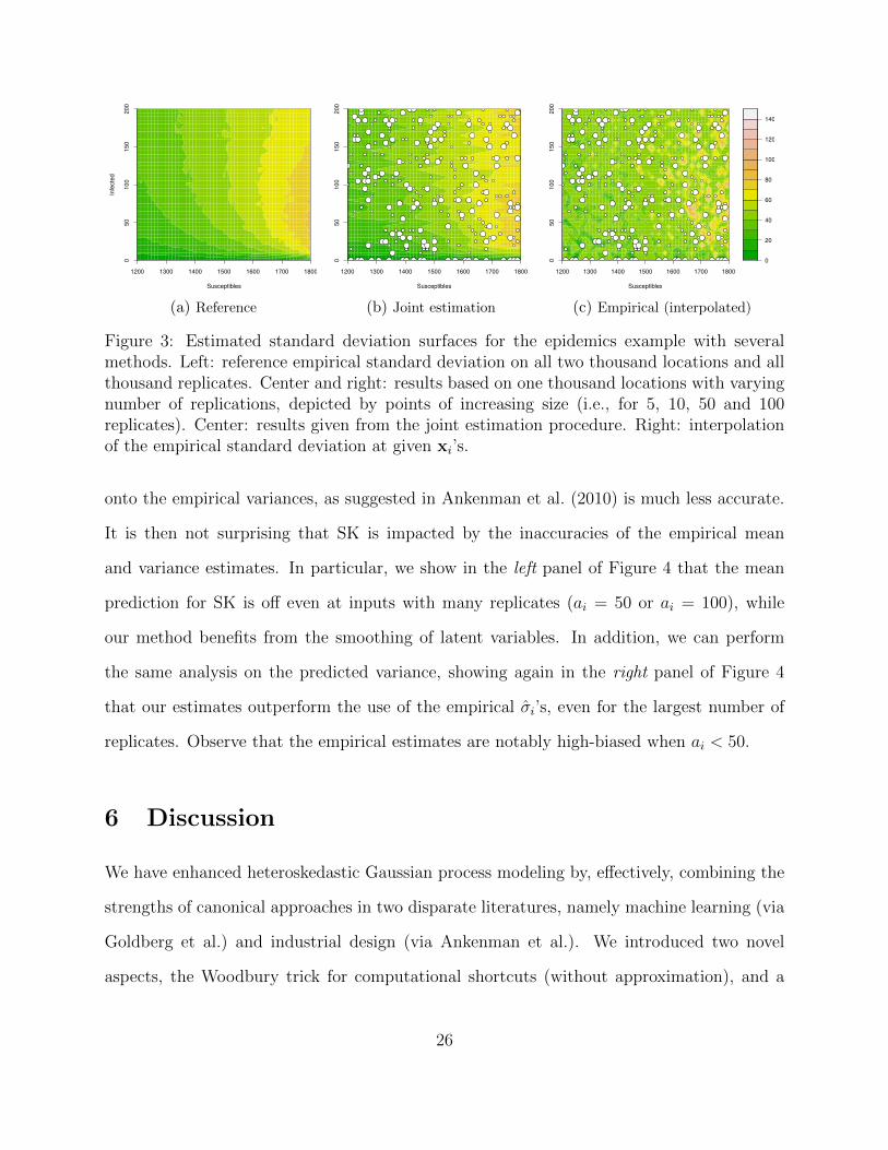
The counterpart of Figure 6 in Hu and Ludkovski (2017) is Figure 3 here. Our proposed

method recovers the key features of the variance surface, with a significantly lower number

of replicates. As a comparison (see rightmost panel), an interpolating model directly fit

25

1200 1300 1400 1500 1600 1700 1800

050

100

150

200

Susceptibles

Infe

cted

(a) Reference

1200 1300 1400 1500 1600 1700 1800

050

100

150

200

Susceptibles

(b) Joint estimation

0

20

40

60

80

100

120

140

1200 1300 1400 1500 1600 1700 1800

050

100

150

200

Susceptibles

(c) Empirical (interpolated)

Figure 3: Estimated standard deviation surfaces for the epidemics example with severalmethods. Left: reference empirical standard deviation on all two thousand locations and allthousand replicates. Center and right: results based on one thousand locations with varyingnumber of replications, depicted by points of increasing size (i.e., for 5, 10, 50 and 100replicates). Center: results given from the joint estimation procedure. Right: interpolationof the empirical standard deviation at given xi’s.

onto the empirical variances, as suggested in Ankenman et al. (2010) is much less accurate.

It is then not surprising that SK is impacted by the inaccuracies of the empirical mean

and variance estimates. In particular, we show in the left panel of Figure 4 that the mean

prediction for SK is off even at inputs with many replicates (ai = 50 or ai = 100), while

our method benefits from the smoothing of latent variables. In addition, we can perform

the same analysis on the predicted variance, showing again in the right panel of Figure 4

that our estimates outperform the use of the empirical σi’s, even for the largest number of

replicates. Observe that the empirical estimates are notably high-biased when ai < 50.

6 Discussion

We have enhanced heteroskedastic Gaussian process modeling by, effectively, combining the

strengths of canonical approaches in two disparate literatures, namely machine learning (via

Goldberg et al.) and industrial design (via Ankenman et al.). We introduced two novel

aspects, the Woodbury trick for computational shortcuts (without approximation), and a

26

−40

−20

0

20

40

60

Y, d

epar

ture

from

refe

renc

e

−40

−20

0

20

40

60

−40

−20

0

20

40

60

−40

−20

0

20

40

60

training testing

Emp w/ 5

WHet w/ 5

SK w/ 5

Emp w/ 1

0

WHet w/ 1

0

SK w/ 10

Emp w/ 5

0

WHet w/ 5

0

SK w/ 50

Emp w/ 1

00

WHet w/ 1

00

SK w/ 100

WHet SK

−40

−20

0

20

40

60

σ2, d

epar

ture

from

refe

renc

e

−40

−20

0

20

40

60

−40

−20

0

20

40

60

training testing

SK & Emp w/ 5

WHet w/ 5

SK & Emp w/ 1

0

WHet w/ 1

0

SK & Emp w/ 5

0

WHet w/ 5

0

SK & Emp w/ 1

00

WHet w/ 1

00WHet

Figure 4: Boxplot of difference between reference mean (left panel) and reference standarddeviation (right panel) obtained on all data with, on a subset of locations and replicates,the empirical mean (Emp, white), the results given by Stochastic Kriging (SK, blue) andthose of our method (WHet, red). Results are separated by the number of replicates in thetraining set (5 to 100), as well as comparison on the testing set (extreme right).

smoothed latent process in lieu of expensive EM and MCMC simulation-based alternatives

to inference. The result is an inferential framework that upgrades modeling fidelity—input-

dependent noise—while retaining a computational complexity on par with the best imple-

mentations of constant noise GP methods. Appendix C explores how our approach copes

well with other types of non-stationarity, despite the model mismatch.

In our survey of the literature we discovered a connection between the Woodbury trick

and an approximate method of circumventing big data (homoskedastic) GP calculations via

pseudo inputs (Snelson and Ghahramani, 2005) and the so-called predictive process Banerjee

et al. (2008). Those methods, rather than leveraging replicates, approximates a big data

spatial field with a smaller latent process: the inputs, outputs, and parameters for which

are jointly inferred in a unified optimization (pseudo-inputs) or Bayesian (predictive pro-

cess) framework. Indeed the spirit of pseudo-input version is similar to ours, being almost

identical when restricting the latent process to the coordinates of the unique-n inputs X in

27

the homoskedastic modeling setup. Snelson and Gharamani (2006) and later Kersting et al.

(2007) proposed heteroskedastic pseudo-inputs variants, with raw optimization of the latents

rather than via the smoothing process that we propose. An advantage of free estimation of

the pseudo inputs, i.e., rather than fixing them to X as we do, is that additional computa-

tional savings can be realized in situations where replication is infeasible or undesired, albeit

by approximation and assuming that the pseudo-inputs can be selected efficiently. We see

tremendous potential for further hybridization of our approach with the wider literature on

approximate (heteroskedastic) modeling of GP in big data contexts.

Acknowledgments

All three authors are grateful for support from National Science Foundation grants DMS-

1521702 and DMS-1521743. Many thanks to Peter Frazier for suggesting the ATO problem.

A Supporting replication

The subsections below provide some of the details that go into lemmas involving the Wood-

bury trick for efficient inference and prediction with designs under replication, followed by

an empirical illustration of the potential computational savings using our library routines.

A.1 Derivations supporting lemmas in Section 3

Due to the structure of replicates, it follows that U>U = An, Ankn(x) = U>k(x), Ukn(x) =

k(x). Moreover, AnY = U>Y, U>ΣN = ΣnU>, UΣn = ΣNU, AnΣn = U>ΣNU (formu-

28

las with ΣN work with Σ−1N as well). Woodbury’s identity gives (4):

kn(x)>(Kn + A−1n Σn)−1Y = kn(x)>Σ−1

n AnY − kn(x)>AnΣ−1n (K−1

n + AnΣ−1n )−1Σ−1

n AnY

= kn(x)>Σ−1n U>Y − k(x)>UΣ−1

n (K−1n + AnΣ

−1n )−1Σ−1

n U>Y

= kn(x)>U>Σ−1N Y − k(x)>Σ−1

N U(K−1n + AnΣ

−1n )−1U>Σ−1

N Y

= k(x)>Σ−1N Y − k(x)>Σ−1

N U(K−1n + U>Σ−1

N U)−1U>Σ−1N Y = k(x)>(K + ΣN)−1Y.

The calculations are the same when replacing Y by kn(x) on the right. On the other hand,

having Y on both sides yields:

Y>(KN + ΣN)−1Y = Y>Σ−1N Y −Y>Σ−1

N U(K−1n + U>Σ−1

N U)−1U>Σ−1N Y

= Y>Σ−1N Y −Y>UΣ−1

n (K−1n + AnΣ

−1n )−1Σ−1

n U>Y

= Y>Σ−1N Y − Y>AnΣ

−1n (K−1

n + AnΣ−1n )−1Σ−1

n AnY

= Y>Σ−1N Y − Y>AnΣ

−1n Y + Y>(Kn + A−1

n Σn)−1Y.

The determinant is similar:

log |K + ΣN | = log |K−1n + U>Σ−1

N U|+ log |Kn|+ log |ΣN |

= log |Kn|+ log |K−1n + AnΣ

−1n |+

n∑i=1

ai log Σi

= log |Kn + A−1n Σn|+

n∑i=1

[(ai − 1) log Σi + log ai]

= log |Kn + A−1n Σn|+ log |ΣN | − log |A−1

n Σn|.

29

A.2 Empirical demonstration of Woodbury speedups

The R code below sets up a design in 2-d and evaluates the response as y(x) = x1 exp{−x21−

x22) (Gramacy, 2007), observed with N (0, 0.012) noise. Our example in Appendix C provides

a visual [in Figure 7] of this response in a slightly different context. The design has n = 100

unique space-filling locations, where their degree of replication is determined uniformly at

random in {1, . . . , 50} so that, on average, there are N = 2500 total elements in the design.

R> library(lhs)

R> Xbar <- randomLHS(100, 2)

R> Xbar[,1] <- (Xbar[,1] - 0.5)*6 + 1

R> Xbar[,2] <- (Xbar[,2] - 0.5)*6 + 1

R> ytrue <- Xbar[,1] * exp(-Xbar[,1]^2 - Xbar[,2]^2)

R> a <- sample(1:50, 100, replace=TRUE)

R> N <- sum(a)

R> X <- matrix(NA, ncol=2, nrow=N)

R> y <- rep(NA, N)

R> ybar <- rep(NA, 100)

R> nfill <- 0

R> for(i in 1:100) {

+ X[(nfill+1):(nfill+a[i]),] <-

+ matrix(rep(Xbar[i,], a[i]), ncol=2, byrow=TRUE)

+ y[(nfill+1):(nfill+a[i])] <- ytrue[i] + rnorm(a[i], sd=0.01)

+ ybar[i] <- mean(y[(nfill+1):(nfill+a[i])])

+ nfill <- nfill + a[i]

+ }

Below, we use the homoskedastic modeling function mleHomGP from our hetGP package in

two ways. First, we use it as intended, with the Woodbury trick, saving the the wall time.

R> eps <- sqrt(.Machine$double.eps)

R> Lwr <- rep(eps,2)

R> Upr <- rep(10,2)

R> un.time <- system.time(un <- mleHomGP(list(X0=Xbar, Z0=ybar,

+ mult=a), y, Lwr, Upr))[3]

Then, we use exactly the same function, but with arguments that cause the Woodbury trick

to be bypassed—essentially telling the implementation that there are no replicates.

30

R> fN.time <- system.time(fN <- mleHomGP(list(X0=X, Z0=y,

+ mult=rep(1,N)), y, Lwr, Upr))[3]

First, lets compare times.

R> c(fN=fN.time, un=un.time)

## fN.elapsed un.elapsed

## 432.281 0.093

Observe that the Woodbury trick version is more than 4000 times faster. This experiment

was run an eight-core Intel i7 with 32 GB of RAM with R’s default linear algebra libraries

(i.e., not the threaded MKL library used for ATO experiment in Section 5.2).

Just to check that both methods are performing the same inference, the code chunk below

prints the pairs of estimated lengthscales θ to the screen.

R> rbind(fN=fN$theta, un=un$theta)

## [,1] [,2]

## fN 1.099367 1.789508

## un 1.099308 1.789700

Above we specified the the X input as a list with components X0, Z0 and mult to be explicit

about the mapping between unique-n and full-N representations. However, this is not the

default (or intended) mechanism for providing the design, which is to simply provide a matrix

X. In that case, the implementation first internally calls the find reps function in order to

locate replicates in the design, and build the appropriate list structure for further calculation.

B Supporting heteroskedastic elements

Here we provide derivations supporting our claim that smoothed and optimal solutions

(for latent variables) coincide at the maximum likelihood setting. We then provide a het-

31

eroskedastic example using the hetGP library. Finally, we provide an empirical demonstration

illustrating the consistency of hetGP optimization of the latent variance variables.

B.1 Proof of Lemma 4.1

Proof. Denote (θ∗,∆∗n,φ∗, g∗) as the maximizer of Eq. (18). For simplicity, we work here

with variances and not log variances. By definition, Λ∗n = C(g)Υ−1(g)∆

∗n if and only if

Υ(g)C−1(g)Λ

∗n = ∆∗n. Notice that the top part of (18) is invariant as long as Λn = Λ∗n.

We thus concentrate on the remaining terms: log(ν(g)) and log |Υ(g)|. First, the derivative

of log |Υ(g)| with respect to g is tr(A−1n Υ−1

(g)), which is positive (trace of a positive definite

matrix), hence log |Υ(g)| increases with g; it also does not depend on ∆n. As for log(ν(g)),

nν(g) = ∆∗>n Υ−1(g)∆

∗n ≥ Λ∗>n C−1

(g)Λ∗n since

∆∗>n Υ−1(g)∆

∗n = Λ∗>n C−1

(g)Υ(g)Υ−1(g)Υ(g)C

−1(g)Λ

∗n = Λ∗>n C−1

(g)Λ∗n + gΛ∗>n C−1

(g)A−1n C−1

(g)Λ∗n

and C−1(g)A

−1n C−1

(g) is positive definite. Hence g∗ = 0 and Λ∗n = ∆∗n.

B.2 Illustration in hetGP

The R code below reproduces the key aspects our application of hetGP on the motorcycle

data (available, e.g., in the package MASS Venables and Ripley (2002)), in particular the

bottom row of Figure 1.

R> library(MASS)

R> system.time(het2 <- mleHetGP(mcycle$times, mcycle$accel, lower=15,

+ upper=50, covtype="Matern5_2"))[3]

## elapsed

## 0.641

So it takes about one second to optimize over the unknown parameters, including the latent

32

variances, when linked to R’s default linear algebra libraries. Observe that raw inputs (times)

and responses (accel) are provided, trigging a call to the package’s internal find reps

function to navigate the small amount replication in the design via the Woodbury trick.

The plotting code below generates a pair of plots similar to those in the final row of Figure

1, which we do not duplicate here. Code for other examples, including the more expensive

Monte Carlo experiments for our ATO and SIR examples, is available upon request.

R> Xgrid <- matrix(seq(0, 60, length.out = 301), ncol = 1)

R> p2 <- predict(x=Xgrid, object=het2, noise.var=TRUE)

R> ql <- qnorm(0.05, p2$mean, sqrt(p2$sd2 + p2$nugs))

R> qu <- qnorm(0.95, p2$mean, sqrt(p2$sd2 + p2$nugs))

R> par(mfrow=c(1,2))

R> plot(mcycle$times, mcycle$accel, ylim=c(-160,90), ylab="acc",

+ xlab="time")

R> lines(Xgrid, p2$mean, col=2, lwd=2)

R> lines(Xgrid, ql, col=2, lty=2); lines(Xgrid, qu, col=2, lty=2)

R> plot(Xgrid, p2$nugs, type="l", lwd=2, ylab="s2", xlab="time",

+ ylim=c(0,2e3))

R> points(het2$X0, sapply(find_reps(mcycle[,1],mcycle[,2])$Zlist, var),

+ col=3, pch=20)

B.3 Robustness in numerical optimization

In Section 4.3 we advocate initializing gradient-based optimization of the latent noise vari-

ables using residuals obtained from homogeneous fit, and this is the default in hetGP. To

illustrate that this is a good starting point, difficulties in MLE estimation for GP hyperpa-

rameterization notwithstanding (Erickson et al., 2017), we provide here two demonstrations

that this procedure is efficient. The first example reuses the motorcycle data while the second

is the 2d Branin function (Dixon and Szego, 1978) redefined on [0, 1]2 with i.i.d Gaussian

additive noise with variance: 2 + 2 sin(πx1) cos(3πx2) + 5(x21 + x2

2))). Unique n = 100 de-

sign points have been sampled uniformly, along with uniformly allocated replicates until

N = 1000. The experiments compare the log-likelihood and other estimates obtained via

33

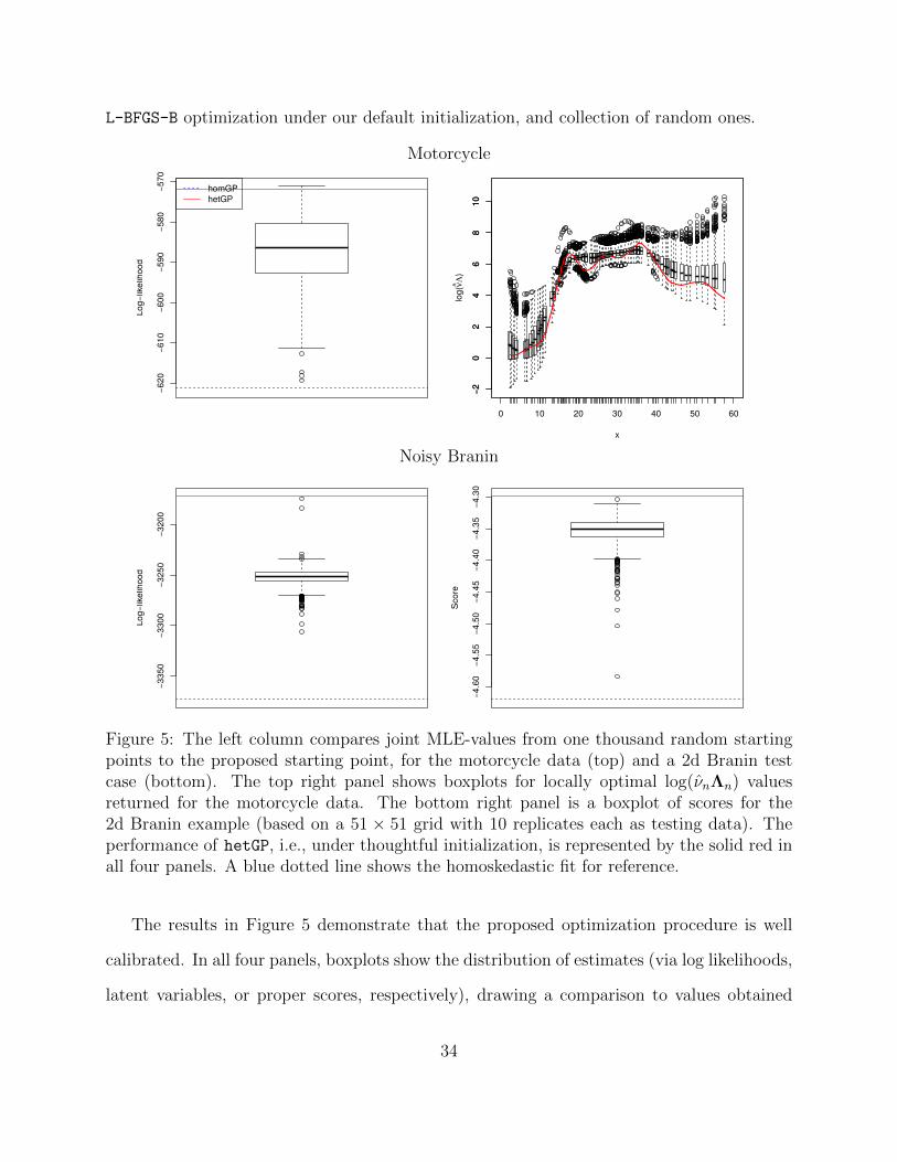
L-BFGS-B optimization under our default initialization, and collection of random ones.

Motorcycle−6

20−6

10−6

00−5

90−5

80−5

70

Log−

likel

ihoo

d

homGPhetGP

0 10 20 30 40 50 60

−20

24

68

10

x

log(νΛ

)

−20

24

68

10

Noisy Branin

−335

0−3

300

−325

0−3

200

Log−

likel

ihoo

d

−4.6

0−4

.55

−4.5

0−4

.45

−4.4

0−4

.35

−4.3

0

Scor

e

Figure 5: The left column compares joint MLE-values from one thousand random startingpoints to the proposed starting point, for the motorcycle data (top) and a 2d Branin testcase (bottom). The top right panel shows boxplots for locally optimal log(νnΛn) valuesreturned for the motorcycle data. The bottom right panel is a boxplot of scores for the2d Branin example (based on a 51 × 51 grid with 10 replicates each as testing data). Theperformance of hetGP, i.e., under thoughtful initialization, is represented by the solid red inall four panels. A blue dotted line shows the homoskedastic fit for reference.

The results in Figure 5 demonstrate that the proposed optimization procedure is well

calibrated. In all four panels, boxplots show the distribution of estimates (via log likelihoods,

latent variables, or proper scores, respectively), drawing a comparison to values obtained

34

under our thoughtful initialization (in solid red), relative to the baseline homoskedastic

fit (blue-dashed). More than 99% of the time our thoughtful initialization leads to better

estimates than under random initialization. The top-right panel, which is in log space, shows

that some latent variable estimates obtained under random initialization are quite egregiously

over-estimated. It is harder to perform such a visualization in 2d, so the bottom-right panel

shows the more aggregated score metric instead.

C Non-stationarity

Input-dependent noise is one form of non-stationarity amongst many. Perhaps the most com-

monly addressed form of non-stationary is in the mean, however the recent literature caters

to many disparate forms (e.g., Gramacy and Lee, 2008; Ba et al., 2012; Snoek et al., 2014;

Gramacy and Apley, 2015; Roininen et al., 2016; Marmin et al., 2017). When there is little

data available, distinguishing between non-stationarity in the mean and heteroskedasticity of

the noise is hard, but even a mis-specified heteroskedastic-only model may be sufficient (i.e.,

better than a purely stationary one) for many tasks. We illustrate this on two examples.

The first one is an univariate sinusoidal function with a jump and the second is the two-

dimensional function of Gramacy (2007), described above in Section A.2. The results are

shown in Figures 6 and 7, respectively. In both cases, the estimated noise increases in areas

where mean dynamics are most rapidly changing. This leads to improved accuracy, and can

facilitate active learning heuristics in sequential design (Gramacy and Lee, 2009). Focusing

design effort in regions of high noise can be useful even if the true explanation is rapidly

changing signal (not high noise). Nevertheless, when the design increases in the “interesting

region”, either through further exploration or a larger number of replicates, this behavior

disappears and a homogeneous model is returned. Investigations on hybrids of noise and

mean heterogeneity represents a promising avenue for future research.

35

● ●

●

●● ●

● ●

●

●

● ●●

●

●

●●

● ●●

●● ●

●

●

●

●

●

●

●

●

● ●

●

●

●●

●●

●

● ●

● ●

●●

●● ●

●●

●●

●

●●

●

●

● ●

●

●

●

●

● ●

●

●●

●

●

●

●● ●

●

●

●● ●

● ● ●

●

●●

●

● ●● ●

●●

0.0 0.2 0.4 0.6 0.8 1.0

−10

−5

05

10

x

f(x)

● ●

● ● ●

●●

●

●

●

●● ●

● ●

●●

●

●●

●

●●

●

●

●

●●

●

● ●

● ●

●

●● ●

● ●

●

●

● ●●

●

●

●●

● ●●

●● ●

●

●

●

●

●

●

●

●

● ●

●

●

●●

●●

●

● ●

● ●

●●

●● ●

●●

●●

●

●●

●

●

● ●

●

●

●

●

● ●

●

●●

●

●

●

●● ●

●

●

●● ●

● ● ●

●

●●

●

● ●● ●

●●

0.0 0.2 0.4 0.6 0.8 1.0

−10

−5

05

10

x

f(x)

● ●

● ● ●

●●

●

●

●

●● ●

● ●

●●

●

●●

●

●●

●

●

●

●●

●

● ●

0 20 40 60 80 100

05

1015

20

x

Noi

se v

aria

nce

Figure 6: Results from a homoskedastic stationary GP (left) and heteroskedastic stationaryGP (center), using the same color code as in Figure 1 based on 31 equidistant points with 3replicates each. Right: estimated variance with heteroskedastic model (red solid line), withhomoskedastic model (blue dashed line) and true unit-variance (black dotted line).

−0.4

−0.2

0.0

0.2

0.4

−2 0 2 4 6

−2

0

2

4

6

0.008

0.010

0.012

0.014

0.016

0.018

−2 0 2 4 6

−2

0

2

4

6

Figure 7: Estimated predictive mean (left) and standard deviation (right) surfaces on thetwo-bumps function Gramacy (2007), based on a 21 × 21 grid with 3 replicates each. Thetrue homogeneous standard deviation used is 10−2.

References

Ankenman, B. E., Nelson, B. L., and Staum, J. (2010). “Stochastic kriging for simulation

metamodeling.” Operations Research, 58, 371–382.

Ba, S., Joseph, V. R., et al. (2012). “Composite Gaussian process models for emulating

expensive functions.” The Annals of Applied Statistics , 6, 4, 1838–1860.

Banerjee, S., Gelfand, A. E., Finley, A. O., and Sang, H. (2008). “Gaussian predictive

36

process models for large spatial data sets.” Journal of the Royal Statistical Society: Series

B (Statistical Methodology), 70, 4, 825–848.

Binois, M. and Gramacy, R. B. (2017). hetGP: Heteroskedastic Gaussian Process Modeling

and Design under Replication. R package version 1.0.0.

Boukouvalas, A. and Cornford, D. (2009). “Learning heteroscedastic Gaussian processes for

complex datasets.” Tech. rep., Aston University, Neural Computing Research Group.

Core Team, R. (2014). R: A Language And Environment For Statistical Computing . R

Foundation for Statistical Computing, Vienna, Austria.

Dixon, L. and Szego, G. (1978). “The global optimization problem: an introduction.” To-

wards global optimization, 2, 1–15.

Eidsvik, J., Shaby, B. A., Reich, B. J., Wheeler, M., and Niemi, J. (2014). “Estimation and

prediction in spatial models with block composite likelihoods.” Journal of Computational

and Graphical Statistics , 23, 295–315.

Erickson, C. B., Ankenman, B. E., and Sanchez, S. M. (2017). “Comparison of Gaussian

process modeling software.” European Journal of Operational Research.

Gneiting, T. and Raftery, A. E. (2007). “Strictly proper scoring rules, prediction, and

estimation.” Journal of the American Statistical Association, 102, 477, 359–378.

Goldberg, P. W., Williams, C. K., and Bishop, C. M. (1998). “Regression with input-

dependent noise: A Gaussian process treatment.” In Advances in Neural Information

Processing Systems , vol. 10, 493–499. Cambridge, MA: MIT press.

Gramacy, R. and Lee, H. (2009). “Adaptive Design and Analysis of Supercomputer Experi-

ment.” Technometrics , 51, 2, 130–145.

37

Gramacy, R. B. (2007). “tgp: an R package for Bayesian nonstationary, semiparametric

nonlinear regression and design by treed Gaussian process models.” Journal of Statistical

Software, 19, 9, 6.

Gramacy, R. B. and Apley, D. W. (2015). “Local Gaussian process approximation for large

computer experiments.” Journal of Computational and Graphical Statistics , 24, 2, 561–

578.

Gramacy, R. B. and Lee, H. K. H. (2008). “Bayesian Treed Gaussian Process Models With

an Application to Computer Modeling.” Journal of the American Statistical Association,

103, 483, 1119–1130.

Haaland, B. and Qian, P. (2011). “Accurate emulators for large-scale computer experiments.”

Annals of Statistics , 39, 6, 2974–3002.

Harville, D. (1997). Matrix algebra from a statistician’s perspective. Springer-Verlag.

Hong, L. and Nelson, B. (2006). “Discrete optimization via simulation using COMPASS.”

Operations Research, 54, 1, 115–129.

Hu, R. and Ludkovski, M. (2017). “Sequential design for ranking response surfaces.”

SIAM/ASA Journal on Uncertainty Quantification, 5, 1, 212–239.

Kaminski, B. (2015). “A method for the updating of stochastic Kriging metamodels.” Eu-

ropean Journal of Operational Research, 247, 3, 859–866.

Kaufman, C., Bingham, D., Habib, S., Heitmann, K., and Frieman, J. (2012). “Efficient

emulators of computer experiments using compactly supported correlation functions, with

an application to cosmology.” Annals of Applied Statistics , 5, 4, 2470–2492.

38

Kersting, K., Plagemann, C., Pfaff, P., and Burgard, W. (2007). “Most likely heteroscedastic

Gaussian process regression.” In Proceedings of the International Conference on Machine

Learning , 393–400. New York, NY: ACM.

Lazaro-Gredilla, M. and Titsias, M. (2011). “Variational heteroscedastic Gaussian process

regression.” In Proceedings of the International Conference on Machine Learning , 841–848.

New York, NY: ACM.

Lee, M. R. and Owen, A. B. (2015). “Single Nugget Kriging.” Tech. rep., Stanford University.

ArXiv:1507.05128.

Ludkovski, M. and Niemi, J. (2010). “Optimal dynamic policies for influenza management.”

Statistical Communications in Infectious Diseases , 2, 1, article 5.

Marmin, S., Ginsbourger, D., Baccou, J., and Liandrat, J. (2017). “Warped Gaussian pro-

cesses and derivative-based sequential design for functions with heterogeneous variations.”

Merl, D., Johnson, L. R., Gramacy, R. B., and Mangel, M. (2009). “A statistical framework

for the adaptive management of epidemiological interventions.” PloS One, 4, 6, e5807.

Ng, S. H. and Yin, J. (2012). “Bayesian kriging analysis and design for stochastic systems.”

ACM Transations on Modeling and Computer Simulation (TOMACS), 22, 3, article no. 17.

Nychka, D., Bandyopadhyay, S., Hammerling, D., Lindgren, F., and Sain, S. (2015). “A

Multi-resolution Gaussian process model for the analysis of large spatial data sets.” Journal

of Computational and Graphical Statistics , 24, 2, 579–599.

Opsomer, J., Ruppert, D., Wand, W., Holst, U., and Hossler, O. (1999). “Kriging with

nonparameteric variance function estimation.” Biometrics , 55, 704–710.

39

Picheny, V. and Ginsbourger, D. (2013). “A nonstationary space-time Gaussian process

model for partially converged simulations.” SIAM/ASA Journal on Uncertainty Quantifi-

cation, 1, 57–78.

Plumlee, M. (2014). “Efficient inference for random fields using sparse grid designs.” Journal

of the American Statistical Association, 109, 508, 1581–1591.

Quadrianto, N., Kersting, K., Reid, M., Caetano, T., and Buntine, W. (2009). “Kernel

conditional quantile estimation via reduction revisited.” In Proceedings of the 9th IEEE

International Conference on Data Mining , 938–943.

Roininen, L., Girolami, M., Lasanen, S., and Markkanen, M. (2016). “Hyperpriors for Matern

fields with applications in Bayesian inversion.” arXiv preprint arXiv:1612.02989 .

Roustant, O., Ginsbourger, D., and Deville, Y. (2012). “DiceKriging, DiceOptim: Two R

Packages for the analysis of computer experiments by kriging-based metamodeling and

optimization.” Journal of Statistical Software, 51, 1, 1–55.

Snelson, E. and Ghahramani, Z. (2005). “Sparse Gaussian processes using pseudo-inputs.”

In Advances in Neural Information Processing Systems , 1257–1264.

Snelson, E. and Gharamani, Z. (2006). “Variable noise and dimensionality reduction in Gaus-

sian processes.” In Proceedings of the International Conference in Artificial Intelligence.

Also see arXiv:1506.04000.

Snoek, J., Swersky, K., Zemel, R. S., and Adams, R. P. (2014). “Input Warping for Bayesian

Optimization of Non-stationary Functions.” In International Conference on Machine

Learning , 1674–1682.

Venables, W. N. and Ripley, B. D. (2002). Modern Applied Statistics with S . 4th ed. New

York: Springer. ISBN 0-387-95457-0.

40

Wang, W. and Chen, X. (2016). “The effects of estimation of heteroscedasticity on stochastic

kriging.” In Proceedings of the 2016 Winter Simulation Conference, 326–337. IEEE Press.

Xie, J., Frazier, P., and Chick, S. (2012). “Assemble to Order Simulator.”

41