practical fiber weave effect modeling - smt & surface mount

Copyright © LAMSIM Enterprises Inc.

Practical Fiber Weave Effect Modeling

White Paper-Issue 2

Lambert Simonovich

1/10/2011

Fiber weave effect is becoming more of an issue as bit rates continue to sore upwards to 5GB/s and

beyond. Due to the non-homogenous nature of printed circuit board laminates, the fiberglass weave

pattern causes signals to propagate at different speeds within differential pair traces; causing timing skew

and mode conversion at the receiver; leading to reduced bit-error-rate (BER) performance; and increased

EMI radiation. The relative dielectric constant (Dk) surrounding a trace ultimately determines its

propagation delay. This paper delves into the issue and presents a novel approach to practically establish

worst case min/max values for Dk and use them to model this effect using Agilent EEofEDA circuit

modeling software. A PCIe CEM Rev2 case study is used to practically demonstrate the model and to

explore the design space.

©LAMSIM Enterprises Inc.

2

This page is intentionally left blank


3

PRACTICAL FIBER WEAVE EFFECT MODELING

Fiber weave effect is becoming more of an issue as bit rates continue to sore upwards. For signalling rates

of 5GB/s and beyond, it can actually ruin your day.

So what is fiber weave effect anyways? Well, it is the term commonly used when a fiberglass reinforced

dielectric substrate causes timing skew between two or more transmission lines of the same length. Since

the dielectric material used in the PCB fabrication process is made up of fiberglass yarns woven into cloth

and impregnated with epoxy resin, it becomes non-homogenous. When one trace happens to line up over

a bundle of glass yarns for a portion of its length as illustrated in Figure 2, it will have a different

propagation delay compared to another trace of the same length which lines up over mostly resin. This is

known as timing or phase skew.

Modern serial link interfaces use differential signalling on a pair of transmission lines of equal length for

interconnect between two points. Any timing skew between the positive (D+) and negative (D-) data will

convert some of the differential signal into a common signal component. Ultimately this results in eye

closure at the receiver and contributes to Electro-Magnetic Interference (EMI) radiation.

Figure 1 5GB/s received eye after 30 inches is entirely closed with 12.7 inches of fiber weave effect. Modeled and

simulated using Agilent ADS.


4

The speed at which a signal propagates along a transmission line depends on the material’s relative

permittivity (er) also known as dielectric constant (Dk). The higher the Dk, the slower the signal

propagates along the transmission line. Knowing the Dk, the propagation delay can be determined using

Equation 1. Since the fiberglass yarn has a higher Dk than resin, maximum intra-pair timing skew will

occur for the section shown in Figure 2.

Equation 1

Where:

tpd = propagation delay in seconds per inch.

er = relative permittivity or dielectric constant Dk. In micro-stripline this is the effective Dk due to the

combination of air and material dielectric.

c = speed of light = 2.998E+8 m/s (1.18E+10 in/s)

In 2005 Intel formed an internal Fiber weave Work Group. Its mandate was to “define Intel’s short and

long-term strategies for dealing with the negative signal integrity effects of fiber weave in the materials

which circuit boards are made of.” For the next couple of years, they compiled over 58,000 TDR and

TDT measurements from hundreds of test boards using different laminates and fabricators. In 2007, Jeff

Loyer et al [3] presented a DesignCon paper “Fiber Weave Effect: Practical Impact Analysis and

Fiber Weave Effect

Figure 2 Fiber weave effect example of differential pair routing showing one trace routed over a fiberglass bundle for a

portion of its length while the other trace is routed over mostly resin


5

Mitigation Strategies” where they published the data and proposed techniques to mitigate the effect of

fiber weave skew.

The statistical data revealed a mean differential timing skew of 3.85ps/in with a standard deviation

(sigma) of 4.15ps/in. About 99.7% of the data values were within 3sigma from the mean, or 16.3 ps/in.

This represents +/- 8.1 ps/in variation from the nominal propagation delay. Intel adopted a cut-off as 15

ps/in which translated into 0.8 delta Dk worst case variation between the D+ and D- of the differential

pair.

If we step back for a moment and think about this a little bit more, we can actually gain some intuition

and validate the 0.8 number derived from measurements by studying the material properties available

from PCB laminate suppliers. Consider two extreme styles of fiberglass cloths used in modern PCB

laminate construction as illustrated in Figure 3. The loose weave of 106 has the highest resin content of

all the most popular weaves, while the tight weave of 7628 has the lowest. Higher resin content translates

to a lower Dk. Therefore, using both values of Dk should give the maximum delta Dk variation to model

the fiber weave effect.

We can get these numbers from laminate supplier’s data sheets. Fortunately, Park-Nelco [1] provides a

useful dielectric calculator from their web site. By plugging in the fibreglass style and single sheet

thickness, you can get a summary of all the dielectric constants and loss tangents for every family of

dielectric they provide as summarized in Figure 4. For 106 materials, the mean Dk = 3.44 with a sigma of

0.28 for the shaded population. For 7628, the mean Dk = 4.16 with a sigma of 0.25. When you subtract

the two means and sigmas from one another, you get a delta Dk of 0.72 with a sigma of 0.03. At a worse

case 3 sigma, delta Dk can be specified as 0.72 +/- 0.09 so the max delta Dk would be 0.81 which agrees

very well with Intel’s results!

106 Weave 7628 Weave

Figure 3 Illustration of two different styles of fiberglass cloth. The 106 weave on the left shows high resin content

compared to 7628 weave on the right. A higher resin content means a lower average Dk. Weaves with high resin content

like 106 will ultimately be worse for fiber weave effect.


6

Determining Stack-up Specific Dkmin/max

There are two methods you can use to estimate the appropriate min/max values of Dk to use in a

simulation model. Method-1 is the simplest. It involves using the data sheets for 106 and 7628 styles in

the family of dielectric material used in the stack-up. For example, if the stack-up uses standard FR4

material, like N4000-6, you would take the average Dk of 106 and 7628 styles across the frequency from

each data sheet. Afterwards you can calculate Dkmin/max using the following equations:

Equation 2

Equation 3

Where:

Dkmin = average Dk of 106 style prepreg minus one half of the 3 sigma tolerance (0.09)

Dkmax = average Dk of 7628 style prepreg plus one half of the 3 sigma tolerance (0.09)

Method-2 uses the statistical data from Intel. By using Equation 1 to calculate the nominal propagation

delay, tpdnom, and applying +/-8.1ps worst case timing skew, Dkmin/max can be calculated by the following

equations:

Equation 4

Style 106 1MHz 1GHz 2.5GHz 10GHz

Material Dk Dk Dk Dk

N4000-2 3.83 3.61 3.62 3.59

N4000-6FC 3.83 3.61 3.62 3.59

N4000-7 4.12 3.67 3.55 3.51

N4000-11 3.77 3.53 3.50 3.51

N4000-12 3.40 3.28 3.17 3.16

N4000-12SI 3.41 3.17 3.26 3.22

N4000-13 3.53 3.29 3.29 3.25

N4000-13SI 3.25 3.14 3.12 3.11

N4000-29 4.09 3.88 3.72 3.71

N5000 3.69 3.12 3.31 3.26

N7000-1 3.74 3.46 3.50 3.48

N7000-2HT 3.16 3.12 2.86 2.83

N8000 3.65 3.35 3.30 3.34

Mean= 3.44

Standard Deviation= 0.28

Style 7628 1MHz 1GHz 2.5GHz 10GHz

Material Dk Dk Dk Dk

N4000-2 4.58 4.42 4.18 4.15

N4000-6FC 4.58 4.42 4.18 4.15

N4000-7 4.64 4.17 4.06 4.05

N4000-11 4.42 4.18 3.76 3.76

N4000-12 4.14 3.92 3.84 3.85

N4000-12SI n/a n/a n/a n/a

N4000-13 4.10 3.99 3.90 3.90

N4000-13SI n/a n/a n/a n/a

N4000-29 4.77 4.54 4.27 4.27

N5000 4.39 4.36 3.80 3.79

N7000-1 4.55 4.16 4.10 4.11

N7000-2HT 4.30 4.19 3.95 3.94

N8000 4.17 4.14 3.93 3.96

Mean= 4.16

Standard Deviation= 0.25

Figure 4 Summary of dielectric constants for 106 and 7628 weaves for each family of dielectric laminates from Park Nelco

dielectric calculator.


7

Equation 5

Where:

Dknom = average value of dielectric constant used in the PCB stack-up geometry

c = speed of light = 2.998E+8 m/s (1.18E+10 in/s)

Example:

An asymmetrical-stripline geometry using N4000-13EP 106 and 1080 style sheets have the properties as

shown in Figure 5.

Method-1:

Method-2:

1x106/1x1080

1x106/1x1080

1x106/1x1080

Core

Prepreg

Prepreg Material 1MHz 1GHz 2.5GHz 10GHz Avg

N4000-13EP Dk Dk Dk Dk Dk

106 3.53 3.29 3.29 3.25 3.34

7628 4.10 3.99 3.90 3.90 3.97

106/1080 3.74 3.55 3.52 3.49 3.58

Figure 5 Example differential pair asymmetrical-stripline geometry showing dielectric layers made up from 106/1080

style sheets relative to diff pair.


8

Both methods give a delta Dk of approximately 0.7, but there are slight differences between the min and

max Dk. Method-2 assumes an equal timing skew of +/-8.1 ps/in because it is half of the worst case

timing skew of 16.2ps/in reported from Intel’s results. In reality though, this is rarely the case. Therefore,

Method-1 is the preferred choice from a practical modeling perspective. Method-2 can be used to as a

double check to validate the results.

Intra-pair Skew Induced Differential Insertion Loss

Intra-pair timing skew in a differential path will cause an increase in the differential insertion loss profile

due to timing induced resonances [4] as shown in Figure 6. In this example, there is 65.2 ps of timing

skew over 4 inches of trace which causes the resonant frequency null at about 7.8 GHz. You can predict

the resonant frequency if you know the total intra-pair timing skew using the following equation:

Equation 6

Where:

= resonant frequency

= total intra-pair timing skew

An intra-pair timing skew of 65.2 ps substituted into Equation 6 results in a resonant frequency null at 7.7

GHz. Because other nulls occur at every odd harmonic of the resonant frequency, the next frequency null

occurs at the third harmonic or 23 GHz.

Increasing the fiber weave effect length, results in a proportional increase in timing skew leading to a

decrease in the resonant frequency by the same proportion. For example, if you double the intra-pair

timing skew, the resonant frequency will be halved. You will start to see increasing eye closure as the

resonant notch approaches half the bit rate (also known as Nyquist frequency). When this happens, the

eye will be entirely closed as shown in Figure 1.


9

Developing the Modeling Methodology:

Since the variation in timing skew determines the maximum bit rate obtainable on any system, it is

important to model and simulate this effect to establish link budgets and routing rules prior to starting the

PCB layout. This means that the dielectric constant surrounding each half of the differential pair will have

to be different in the model.

You can build a circuit model using Agilent EEsofEDA software [10] as shown in Figure 7 by using the

Multi-layer palette from the drop-down menu in the schematic window. The two balun transformers are

used for convenience to get the mixed mode insertion and return losses. The 25 ohm resistors are used to

terminate the common signal that is present through mode conversion when there is intra-pair timing

skew.

There are two identical multi-layer substrates representing the board stack-up geometry. One substrate

(subst9) uses the lower Dk associated with a high resin area of the material while subst10 uses the higher

Dk due to the fibreglass weave.

Two ML1CTL_C single transmission lines models are used for each trace of the differential pair instead

of a coupled transmission line because ADS requires a coupled transmission line model to share the same

substrate and have the same dielectric constant for both tracks. One transmission line is referenced to

subst9 and the other to subst10.

When a differential pair has no coupling, it behaves like two single-ended traces driven differentially. In

this scenario, Zodd = Zeven = Zo. Single lines can be used as long as you increase the line widths

accordingly so that the characteristic impedance (Zo) of each trace equals the odd mode impedance of a

coupled line. You may also need to adjust the loss tangent for each substrate to match the same insertion

and return losses as a coupled line.

2 4 6 8 10 12 14 16 180 20

-30

-20

-10

-40

0

freq, GHz

Inse

rtio

n L

oss, d

B

___ 65.2 ps skew

___ No skew

Figure 6 Simulated example of timing induced skew resonance in the differential insertion loss profile due to fiber weave

effect using Agilent ADS. The blue trace is with 65.2ps timing skew over 4 inches vs red trace with no timing skew.


10

Fortunately ADS has a tuning tool within the schematic editor allowing you to fine tune the respective

parameters and compare against a coupled line reference model. The reference model is exactly the same

except it uses a single coupled (ML2CTL_C) transmission line and it only has one multi-layer substrate

as shown in Figure 8. The track length, width and space are adjusted accordingly to give the target

differential impedance used in the design. During calibration, Dk and loss tangent (tanD) of all three

substrates are made equal to the nominal values from the dielectric material’s data sheet.

Figure 7 ADS single line circuit model used to model S-parameters of a differential pair of transmission lines.


11

After setting up the parameters, the tuning tool is used to adjust the line width and loss tangent of the

single line model to get a best fit insertion and return loss to the coupled line model. At this stage, the

single line model will be close but not exactly the same as the coupled line model as shown in the

example Figure 9. After calibration, Dk for each substrate is changed back to the min and max values

accordingly. Re-simulate and you should see the effect of the resonant frequency nulls in the insertion and

return loss plots. Figure 10 shows an example with 8.6 inches of fiber weave, a Dkmin/max of 3.30 and 4.02

respectively and Dknom= 3.58. The resonant frequency nulls occur at 3.6GHz, 10.8GHz and 18GHz.

Insertion Loss Return Loss TDR

Figure 9 ADS simulation example results of single line model to reference coupled line model fitting using the tuning tool

within the ADS schematic page.

Figure 8 ADS coupled line reference model (left) vs single line model (right).


12

Exploring Design Space:

You can use this simple method of modeling fiber weave timing skew to quickly explore design space.

For example, the PCI Express® External Cabling Specification, Revision 1.0 worst case skew budget is

21% of a unit interval (U.I.), where one U.I. is equal to the bit time. At 2.5GT/s this works out to 84ps.

On the other hand, the PCIe Card Electromechanical Specification (CEM) Rev. 2.0 does not have a

specification per se other than intra-pair track routing skew of 15 mils. Of this, 5 mils is reserved for the

add-in card; and 10 mils for the system card. If we assume the receiver can tolerate the same 0.21 U.I. of

intra-pair timing skew, this works out to be about 42 ps at 5GT/s.

Using the dielectric data shown in Figure 5 as an example, we can establish the fiber weave effect track

length needed to give 42 ps timing skew based on worst case delta Dk. After using Method-1 to calculate

Dkmin/max, delta tpd is calculated using the following equation:

Equation 7

As you can see, it is easily possible for the two lines making up a differential pair to violate the 42 ps

skew spec after only 2.6 inches.

We can use the single line model of Figure 7 to explore what 0.21 U.I. of intra-pair skew has on insertion

loss and compare it against the PCIe cable spec. The left plot of Figure 11 shows the results after

simulating 2.6 inches of fiber weave effect using the circuit model of Figure 7. This shows us there is

only about 0.5dB additional loss at the Nyquist frequency for 5GT/s. When 5.2 inches is used,

representing 0.21 U.I. at 2.5GT/s, the additional loss is essentially the same as shown in the right plot of

Figure 11.

This tells us two things. First, 0.21 U.I. is a reasonable intra-pair skew budget for PCIe CEM Rev2

applications. But, most importantly, it tells us that if you use 5.2 inches as your budget at 2.5GT/s and

Return Loss TDR Insertion Loss

Figure 10 ADS simulation example of maximum fiber weave effect over 8.6 inches using Dkmin/max of 3.30 and 4.02

respectively compared against reference model using Dk of 3.58. Resonant frequency null, fo= 3.6GHz and odd

harmonics at 10.8GHz and 18GHz respectively.


13

later want to reuse the same PCB for 5GT/s, you will have an additional insertion loss of about 2dB at

2.5GHz Nyquist frequency. Since fiber weave induced skew depends on the random alignment of the

fiber weaves to the tracks, it does not mean the design will not work if the length is 5.2 inches or more.

Because of the statistical nature of the problem, it means that if you build enough boards, you will

experience some sort of degradation. If your channel is close to the limit, it may fail the BER

performance.

PCIe CEM Rev2 Case Study:

We can explore this further by simulating some realistic channel models of practical designs and the

effect it has on Bit Error Rate (BER) performance. The PCIe CEM specification is a companion for the

PCIe Base Specification, Revision 2.0. Its primary focus is for desktop/server mechanical and electrical

specifications. It covers three possible electrical topologies:

PCIe devices on the same board.

PCIe devices on two boards with one connector, one system board and one add-in card.

PCIe devices on three boards with two connectors, one system board, one riser card and one add-

in card.

For this case study, the scenario of PCIe devices on two boards with one connector, one system board and

one add-in card is explored. The link definition is described by Figure 12. The differential trace

impedance for 5GT/s application is 85 ohms for both the system board and add-in card. AC coupling

capacitors are placed at the transmit side of the connector.

2 4 6 8 10 12 14 16 180 20

-30

-20

-10

-40

0

freq, GHz

dB

(S(2

,1))

Readout

m2

dB

(S(4

,3))

Readout

m1

m1ind Delta=dep Delta=-0.452Delta Mode ON

0.000

2 4 6 8 10 12 14 16 180 20

-30

-20

-10

-40

0

freq, GHzd

B(S

(2,1

))

1.200G-869.3m

m2

dB

(S(4

,3))

1200000000.000-1.255

m1

m1ind Delta=dep Delta=-0.471Delta Mode ON

0.000

Insertion Loss for 2.6 inches

intra-pair skew

Insertion Loss for 5.2 inches

intra-pair skew

___ 16 ps/in skew ___ No skew

Figure 11 ADS simulation results of timing induced intra-pair skew due to fiber weave effect. Left plot is the insertion loss

with 16 ps/in timing skew over 2.6 inches representing PCIe CEM Rev2 budget at 5GT/s. Right plot is with 16 ps/in

timing skew over 5.2 inches representing PCIe cable spec Rev1 budget at 2.5GT/s. Both results have about 0.5 dB

additional attenuation at the respective Nyquist frequency.


14

Transmit Compliance Test Setup and Eye Mask Definition:

The PCIe CEM Rev2 spec defines a transmit eye compliance test mask for the system board and add-in

card as illustrated in Figure 13. Compliance testing is done at the PCIe connector used as the demarcation

point. A special test card with 2 inches of trace length, having 85 ohms differential impedance and

terminated with 100 ohms (top figure) is used to test for system board compliance. Similarly, testing the

add-in card (bottom figure) is done on a system test board at the end of 3 inches of trace with the same

differential impedance and termination.

2”- 85 ohm Diff.

Isolated Tracks

System Board

Interconnect

PC

IeC

onn

ecto

r

System Board Under Test Add-in Compliance Test Card

Tx & PKG

2x50 ohms

Rx & PKG

AC Coupling

Capacitors

3”- 85 ohm Diff.

Isolated Tracks

2x50 ohms

PC

IeC

onn

ecto

r

Add-in Card

Interconnect

Max. Prop Delay =750 ps

System Compliance Test Board Add-in Card Under Test

Tx & PKG

Rx & PKG

AC Coupling

Capacitors

300mV

108 ps*

* -No Xtalk

System Board Tx

Eye Mask @5GT/s

380mV

126 ps*

* -No Xtalk

Plug-in Card Tx

Eye Mask @5GT/s

2”- 85 ohm Diff.

Isolated Tracks

System Board

Interconnect

PC

IeC

onn

ecto

r


Tx & PKG

2x50 ohms

Rx & PKG

AC Coupling

Capacitors

2”- 85 ohm Diff.

Isolated Tracks

System Board

Interconnect

PC

IeC

onn

ecto

r


Tx & PKG

2x50 ohms

Rx & PKG

AC Coupling

Capacitors

3”- 85 ohm Diff.

Isolated Tracks

2x50 ohms

PC

IeC

onn

ecto

r

Add-in Card

Interconnect



Tx & PKG

Rx & PKG

AC Coupling

Capacitors

3”- 85 ohm Diff.

Isolated Tracks

2x50 ohms

PC

IeC

onn

ecto

r

Add-in Card

Interconnect



Tx & PKG

Rx & PKG

AC Coupling

Capacitors

300mV

108 ps*

* -No Xtalk

System Board Tx

Eye Mask @5GT/s

300mV

108 ps*

* -No Xtalk

System Board Tx

Eye Mask @5GT/s

380mV

126 ps*

* -No Xtalk

Plug-in Card Tx

Eye Mask @5GT/s

380mV

126 ps*

* -No Xtalk

Plug-in Card Tx

Eye Mask @5GT/s

PC

IeC

onn

ecto

r

Add-in Card

Interconnect


System Board

Interconnect

System Board Add-in Card

Tx & PKG

Tx & PKG

Rx & PKG

Rx & PKG

AC Coupling

Capacitors

PC

IeC

onn

ecto

r

Add-in Card

Interconnect


Add-in Card

Interconnect


System Board

Interconnect

System Board

Interconnect

System Board Add-in Card

Tx & PKG

Tx & PKG

Rx & PKG

Rx & PKG

AC Coupling

Capacitors

Figure 12 PCIe CEM Rev2 link topology of system board and add-in card. Maximum add-in card differential data trace

propagation delay is 750 ps. For Dk = 3.58, maximum interconnect = 4.7 inches.

Figure 13 PCIe CEM Rev2 transmit eye compliance test setup and transmit masks for system board (top) and plug-in

card (bottom).


15

System Simulation Circuit Model:

Using ADS, we can easily model the PCIe CEM compliance channel calibration methodology by using

the circuit model shown in Figure 14. The circuit uses the “Simulation-ChannelSim” palette from the

drop-down menu in the schematic window for the Tx_Diff differential transmitters and EyeDiff_Probes.

The top left half of the schematic models the system board and uses the same single line models as

described in Figure 7. Line widths need to be adjusted for 85 ohms using nominal Dk = 3.58. Similarly,

the bottom right half of the schematic models the add-in card. The top right and bottom left halves model

the 2 inch and 3 inch single line 85 ohm differential traces respectively. Both are terminated in 100 ohms

differential. A 4-port S-parameter touchstone model of a PCIe_Connector (X14) is used between the two

and is pushed into a hierarchy block.

Both transmitter parameters are set to +/-800 mV, 5GB/s, 8B10 coding. The rise/fall times are set to 30

ps. The system board’s transmitter does not uses de-emphasis while the add-in card uses 3.5dB de-

emphasis as per specification. No jitter parameters are used for the test.

Each half is simulated separately by disabling the opposite transmitter and eye probe. The system board’s

interconnect length is tuned so that the eye opening meets the worst case transmit eye mask as defined in

Figure 13. For the PCB stack-up geometry and line width used in this model example, the system board’s

length is 25 inches. PCIe CEM Rev2 specifies a maximum propagation delay of the differential

interconnect on the add-in card to be 750 ps or less. For a nominal Dk of 3.58, the length is 4.7 inches.

After calibration, we can perform sensitivity analysis to further explore what fiber weave effect has on

system performance. To do this, the top right 2 inch and bottom left 3 inch transmission lines are replaced

with parameterized circuit models similar to the one shown in Figure 15. The fiber weave section uses

the same model as Figure 7 and its length is set by the variable “track_length”. The other section uses

other variables and equations to automatically adjust its length to equal the difference between the total

length and the fiber weave length.

The completed system circuit model schematic is shown in Figure 16. The maximum add-in card

interconnect under test (top right) is set to 4.7 inches as defined by the PCIe CEM rev2 spec. For this

example, the maximum system board interconnect under test (bottom right) is set to 25 inches which is

the same length as determined by the transmit calibration procedure.

To test the add-in card’s receive channel against the PCIe eye mask at 1x10-12

, the upper half of the circuit

model is simulated with the bottom half disabled. The fiber weave length is adjusted up to the maximum

length and the eye opening is compared against the PCIe CEM Rev2 receive mask. Similarly, the bottom

half tests for receive eye compliance on the system board when fiber weave length is increased.


16

Figure 14 ADS schematic of transmit eye compliance channel test setup showing worst case eye with respective masks for

system board (top) and plug-in card (bottom)


17

Total Track Length

Total Track Length - Fiberweave Length Fiberweave Length

Total Track Length

Total Track Length - Fiberweave Length Fiberweave Length

Figure 15 ADS example of parameterized fiber weave circuit model to facilitate easy adjustment of the appropriate single

line transmission lines for fiber weave effect.


18

Transmit Compliance Simulation Results:

Simulated compliant transmit eyes per Figure 14 for the system board and add-in card are shown in

Figure 17. The eye masks plotted are as defined in Figure 13. The left eye diagram is for the system board

while the right shows the results for the add-in card.

Figure 16 ADS PCIe CEM Rev2 system circuit model. Top half test add-in card’s receive channel while bottom half tests

system board’s receive channel.


19

Add-in Card Receive Compliance Simulation Results:

The upper half of the circuit model of Figure 16 was used to simulate the add-in card’s receive channel

interconnect. Three separate simulations were performed:

No skew

2.6 inches of fiber weave skew representing 0.21 U.I. intra-pair skew at 5GT/s

Maximum fiber weave skew

The results are summarized in Figure 18. They show the respective eye diagrams plotted against the PCIe

5GT/s mask for a BER of 1x10-12

. By observing the eye as the fiber weave length is increased, we see the

eye first becoming more rounded and symmetrical then attenuating. At 2.6 inches of fiber weave skew,

there does not appear to be significant degradation in eye opening other than slight rounding to the right

portion of the eye. Because the maximum skew for the add-in card is limited to 4.7 inches, it is not

enough to close the eye to violate the mask. There appears to be margin, but further processing would be

required to include jitter effects that were not simulated. This is beyond the scope of this paper, but you

would need to do this in a real design before sign-off.

When we observe the insertion loss plots, we can see the corresponding resonant frequency null decrease

as the fiber weave length increases. At 2.6 inches, there is approximately 0.5 dB of additional attenuation

at 2.5GHz while at 4.7 inches the additional loss is about 1.6 dB.

Figure 17 ADS simulated eye diagrams vs transmit compliant eye masks for system board (left) and add-in card (right).

System board has no de-emphasis while add-in card employs 3.5dB de-emphasis.


20

System Board Receive Compliance Simulation Results:

The upper half of the circuit model of Figure 16 was used to simulate the system board’s receive channel

interconnect. Four separate simulations were performed:

No skew

5.6 inches of fiber weave skew representing 0.21U.I. intra-skew at 2.5GT/s.**

7.8 inches of fiber weave skew

12.7 inches of fiber weave skew representing length where fo=2.5GHz

**A length of 5.6 inches was chosen for one of the cases to represent the maximum 0.21 U.I. intra-pair

skew at 2.5GT/s even though the simulation was run at 5GT/s. The intent here was to simulate the case of

a PCIe Gen1 legacy layout originally designed to operate at 2.5GT/s and later wanting to explore it’s

suitability for PCIe CEM Rev2.

The results are summarized in Figure 19. Here we see just how much cleaner and open the eyes are

compared to the add-in card’s simulations due to the 3db of de-emphasis on the transmitter. We also

observe how the eye starts to degrade and distort significantly due to mode conversion after only 5.6

inches of fiber weave skew. At 7.8 inches the eye becomes asymmetrical and is entirely closed at 12.7

inches. There appears to be margin at 7.8 inches, but further processing would be required to include jitter

2 4 6 8 10 12 14 16 180 20

-50

-40

-30

-20

-10

-60

0

freq, GHz

dB

(S(2

,1))

Readout

dB

(S(4

,3))

Readout

ind Delta=dep Delta=1.711E-9Delta Mode ON

0.000

2 4 6 8 10 12 14 16 180 20

-50

-40

-30

-20

-10

-60

0

freq, GHz

dB

(S(2

,1))

Readout

dB

(S(4

,3))

Readout

ind Delta=dep Delta=-0.491Delta Mode ON

0.000

2 4 6 8 10 12 14 16 180 20

-50

-40

-30

-20

-10

-60

0

freq, GHz

dB

(S(2

,1))

Readout

dB

(S(4

,3))

Readout


0.000

0.0 inches Fiber

weave Skew

2.6 inches Fiber

weave Skew

4.7 inches Fiber

weave Skew

Figure 18 ADS simulated results for 3 fiber weave lengths showing eye diagrams at the add-in card’s receiver vs PCIe

5GT/s receive eye mask at 1x10-12 BER. Also shown are respective insertion loss plots with insertion loss marked at

Nyquist frequency.


21

effects that were not simulated. This is beyond the scope of this paper, but you would need to do this in a

real design before sign-off.

2 4 6 8 10 12 14 16 180 20

-50

-40

-30

-20

-10

-60

0

freq, GHz

dB

(S(2

,1))

Readout

dB

(S(4

,3))

Readout

ind Delta=dep Delta=1.725E-9Delta Mode ON

0.000

2 4 6 8 10 12 14 16 180 20

-50

-40

-30

-20

-10

-60

0

freq, GHz

dB

(S(2

,1))

Readout

dB

(S(4

,3))

Readout


0.000

2 4 6 8 10 12 14 16 180 20

-50

-40

-30

-20

-10

-60

0

freq, GHz

dB

(S(2

,1))

Readout

dB

(S(4

,3))

Readout


0.000

2 4 6 8 10 12 14 16 180 20

-50

-40

-30

-20

-10

-60

0

freq, GHz

dB

(S(2

,1))

Readout

dB

(S(4

,3))

Readout


0.000

0.0 inches

Fiber weave

Skew

5.6 inches

Fiber weave

Skew

7.8 inches

Fiber weave

Skew

12.7 inches

Fiber weave

Skew

Figure 19 ADS simulated results for 4 fiber weave lengths showing eye diagrams at the system board’s receiver vs PCIe 5GT/s

receive eye mask at 1x10-12 BER. Also shown are respective insertion loss plots.


22

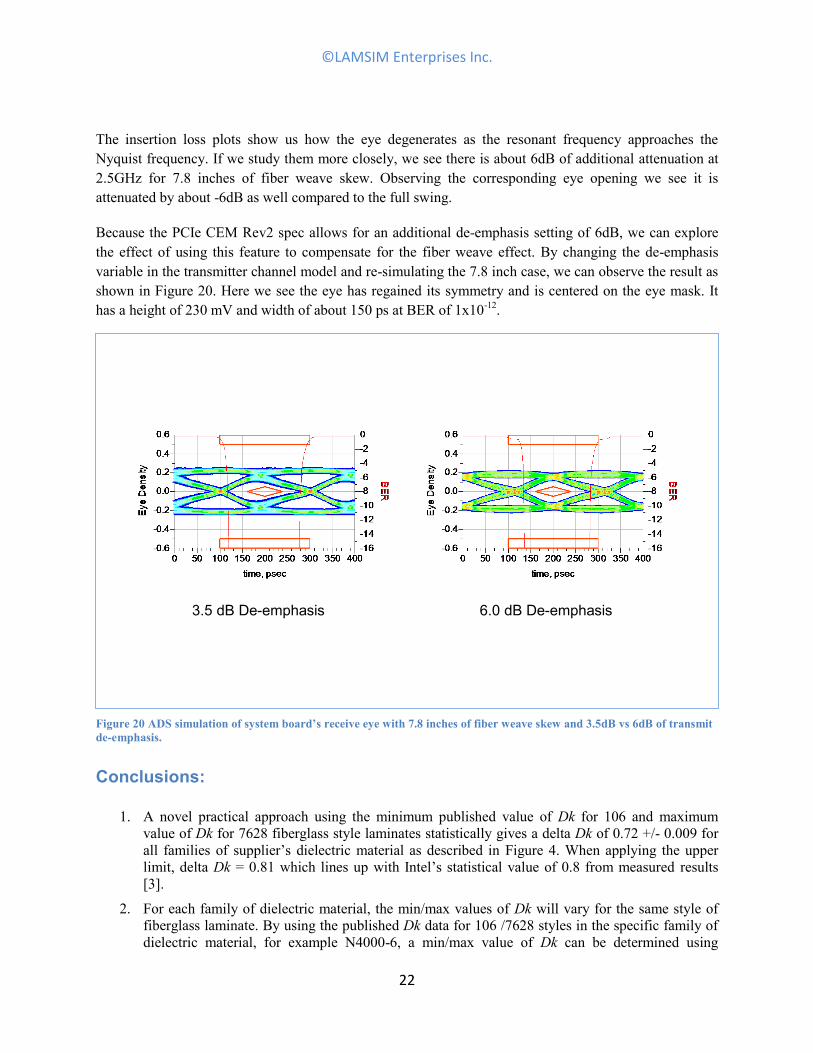
The insertion loss plots show us how the eye degenerates as the resonant frequency approaches the

Nyquist frequency. If we study them more closely, we see there is about 6dB of additional attenuation at

2.5GHz for 7.8 inches of fiber weave skew. Observing the corresponding eye opening we see it is

attenuated by about -6dB as well compared to the full swing.

Because the PCIe CEM Rev2 spec allows for an additional de-emphasis setting of 6dB, we can explore

the effect of using this feature to compensate for the fiber weave effect. By changing the de-emphasis

variable in the transmitter channel model and re-simulating the 7.8 inch case, we can observe the result as

shown in Figure 20. Here we see the eye has regained its symmetry and is centered on the eye mask. It

has a height of 230 mV and width of about 150 ps at BER of 1x10-12

.

Conclusions:

1. A novel practical approach using the minimum published value of Dk for 106 and maximum

value of Dk for 7628 fiberglass style laminates statistically gives a delta Dk of 0.72 +/- 0.009 for

all families of supplier’s dielectric material as described in Figure 4. When applying the upper

limit, delta Dk = 0.81 which lines up with Intel’s statistical value of 0.8 from measured results

[3].

2. For each family of dielectric material, the min/max values of Dk will vary for the same style of

fiberglass laminate. By using the published Dk data for 106 /7628 styles in the specific family of

dielectric material, for example N4000-6, a min/max value of Dk can be determined using

3.5 dB De-emphasis 6.0 dB De-emphasis

Figure 20 ADS simulation of system board’s receive eye with 7.8 inches of fiber weave skew and 3.5dB vs 6dB of transmit

de-emphasis.


23

Equation 2 and Equation 3 respectively. This methodology offers a more realistic approach than

just taking the nominal Dk and applying +/-0.4 for Dkmin/max respectively.

3. An innovative use of Agilent ADS circuit simulation software using the Multi-layer palette and

practical methodology to model fiber weave skew effect has shown it is an excellent tool to

explore design space.

4. The PCIe CEM Rev2 case study has shown that 0.21U.I. is a reasonable number to use for

maximum intra-pair skew budgeting.

5. By taking advantage of transmit de-emphasis in PCIe CEM Rev2 applications it may be possible

to tolerate more than 0.21U.I. intra-pair timing skew in legacy designs.

6. Since fiber weave skew is statistical in nature, it does not mean the system will not work if you

exceed the intra-pair skew budget. The case study example demonstrates that by modeling your

system and applying the min/max variations in Dk, you can sign off on your design with eyes

wide open so to speak. If after all that, your analysis still shows the design is marginal, you can

take it to the next level and apply a host of mitigation strategies listed in Intel’s paper [3].

References:

[1] Park Electrochemical Corp. , http://www.parkelectro.com

[2] Gary Brist et al, “Woven Glass Reinforcement Patterns”, Printed Circuit Design & Manufacture, Nov.

2004

[3] Jeff Loyer et al, “Fiber Weave Effect: Practical Impact Analysis and Mitigation Strategies”

[4] Gustavo Blando et al, “Losses Induced by Asymmetry in Differential Transmission Lines”

[5] Eric Bogatin, http://bethesignal.net/blog, Blog post: “4/9/09 A new glass weave skew solution”

[6] PCI Express®, Base Specification, Revision 2.1, March 4, 2009

[7] PCI Express®, Card Electromechanical, Specification, Revision 2.0, April 11, 2007

[8] PCI Express® External Cabling Specification, Revision 1.0, January 4, 2007

[9] Serial ATA Revision 2.5, 27-October-2005

[10] Agilent Technologies, EEsofEDA, Advanced Design System, 2009 Update1 software.

Biography:

Lambert (Bert) Simonovich Born in Hamilton, Ontario, Canada, graduated in 1976 from Mohawk

College of Applied Arts and Technology in Hamilton, Ontario, Canada as an Electronic Engineering

Technologist. Over a 32 year career at Bell Northern Research and Nortel, he helped pioneer several

advanced technology solutions into products and has held a variety of R&D positions, eventually

specializing in backplane design over the last 25 years. He is the founder of Lamsim Enterprises Inc.

www.lamsimenterprises.com providing innovative signal integrity and backplane solutions. He is

currently engaged in signal integrity, characterization and modeling of high speed serial links associated

with backplane interconnects. He holds two patents and (co)-author of several publications including an

award winning DesignCon2009 paper related to via modeling.

http://www.parkelectro.com/

http://www.lamsimenterprises.com/

practical fiber weave effect modeling - smt & surface mount

Documents