practical computation of axisymmetrical multifluid flows

HAL Id: hal-00139598https://hal.archives-ouvertes.fr/hal-00139598

Submitted on 3 Apr 2007

HAL is a multi-disciplinary open accessarchive for the deposit and dissemination of sci-entific research documents, whether they are pub-lished or not. The documents may come fromteaching and research institutions in France orabroad, or from public or private research centers.

L’archive ouverte pluridisciplinaire HAL, estdestinée au dépôt et à la diffusion de documentsscientifiques de niveau recherche, publiés ou non,émanant des établissements d’enseignement et derecherche français ou étrangers, des laboratoirespublics ou privés.

Practical computation of axisymmetrical multifluid flowsThomas Barberon, Philippe Helluy, Sandra Rouy

To cite this version:Thomas Barberon, Philippe Helluy, Sandra Rouy. Practical computation of axisymmetrical multifluidflows. International Journal on Finite Volumes, Institut de Mathématiques de Marseille, AMU, 2003,1, pp.1-34. hal-00139598

https://hal.archives-ouvertes.fr/hal-00139598

https://hal.archives-ouvertes.fr

ISITV, Laboratoire ANAM/MNC, BP56, 83162 La Valette CEDEX. [email protected]

PRACTICAL COMPUTATION OF AXISYMMETRICAL

MULTIFLUID FLOWS

THOMAS BARBERON, PHILIPPE HELLUY, SANDRA ROUY

Abstract. We adapt the Saurel-Abgrall front capturing finite volumes methodfor an industrial simulation of compressible multifluid flows. We then applythe method to the case of air-water flow in the cooling chamber of an axisym-metrical gas generator. We describe successively how to deal with exact andglobal Riemann solvers, pressure oscillations, unstructured meshes, axisymme-try, boundary conditions and overly restrictive CFL conditions. The resultingalgorithm is efficient and robust.

1. Introduction

This work is devoted to the application of recent finite volumes schemes, andparticularly the one proposed by Saurel and Abgrall in [24], to the simulation ofan axisymmetrical multiphase flow in a complex geometry. Because of the com-plexity of the application, we have to specify or adapt the original Saurel-Abgrallidea to: global Riemann solver, unstructured meshes, axisymmetry, boundary con-ditions, multi time steps...

We base our simulation on an effective mathematical model for compressiblemultifluid flows and especially air-water flows. For our application, the pressurelaw for the air is a classical perfect gas law. Because we have in mind flows withhigh and low pressures, we have also to take into account the compressibility ef-fects in water. In such applications, it is classical to observe cavitation zones inthe liquid phase. Cavitation is a phenomenon that appears in a region of the flowwhere the pressure drops below the saturation pressure of water. In a first and veryshort stage, the liquid stays in a metastable state. It can also happen in this stagethat the pressure becomes negative (it is then called a tension). In a second stage,a phase transition (vaporization) occurs. Thus the original two-phase flow, madeof air and water, becomes a three-phase flow made of air, liquid and vapor. Werestrict ourself to the two-phase case, where the phase transition has not started (oris not taken into account...). Then, as for the air, a pressure law which expressesthe pressure of the water as a function of density and internal energy has to besupplied. We use a very simple generalization of the perfect gas law, the stiffenedgas equation of state (see (2.1)), which allows negative values for the pressure.

Compressible single fluids have been extensively studied and the main difficultyhere is the representation of the interface between the fluids. There are two mainapproaches for treating interfaces:

• One can favor the Lagrangian interpretation of the fluid equations. Theinterface then receives a particular treatment in the numerical method.

Key words and phrases. compressible multifluid, front capturing, nonconservative scheme,axisymmetry.

This work has been supported by a joint research grant DCN/ING Toulon & Region PACA..

1

2 THOMAS BARBERON, PHILIPPE HELLUY, SANDRA ROUY

This approach leads to the family of the front-tracking methods. We willnot consider this kind of solution here.

• If the Eulerian point of view is preferred, the resulting scheme belongs tothe family of the front-capturing methods. No special treatment is appliedto the numerical cells that are crossed by the interface. We prefer the front-capturing methods because they are more general and easier to implementthan the front-tracking methods.

A now classical and simple approach, proposed for example in [22], [19], is to locatethe interface by means of the level-set of a function which is convected with theflow. In this approach only an advection equation has to be added to the classicalcompressible Euler model. One switches from one law (perfect gas) to the other(stiffened gas) according to the value of the level-set function. Because the stiffenedgas law is a generalization of the perfect gas law, the level-set model is also equiva-lent, in our case, to a model where the two coefficients of the stiffened gas law areconvected with the flow. The interface is then located by the discontinuities of thepressure law coefficients. Our model is finally made up of the Euler system (conser-vation of mass, momentum and energy, equations (2.3)), two additional transportequations (equations (2.5)) and the stiffened gas law (equation (2.1)). This mul-tifluid model presents a supplementary transport equation when compared to thelevel-set model but it is generally easier to discretize.

Despite its simplicity and its mathematical perfection, this model leads to nu-merous numerical difficulties as shown in many works among which we can cite[1], [18], [19], [24], [3], [10], [23]... These difficulties have to be overcome beforeenvisaging practical applications. Of greatest concern are the spurious pressure os-cillations that appear near the material interface when the model is approximatedby any conservative finite volumes scheme. The same kind of oscillations occursin the simulation of mixtures of perfect gases [1] or across numerically diffusedshear interfaces [5]. Actually, it appears that classical conservative schemes (suchas Godunov’s, Roe’s, HLL, Rusanov’s, etc.) suffer from a very slow convergenceand a very bad precision on standard meshes when applied to the previous multi-fluid model. Mulder, Osher and Sethian did not mention this fact in [22] althoughthey use in their work a classical conservative Roe scheme. Their trick to obtainacceptable numerical results is not detailed. Karni, in [18], points out this difficultyand proposes a simple hybrid scheme to remove the pressure oscillations. The ideais to solve the classical conservative equations far from the interface between thetwo fluids and a nonconservative pressure equation near the interface. The result-ing nonconservative scheme, which is built in order to preserve constant pressureand velocity states, gives good results. But it is not clear, in the paper of Karni,whether the conservation error tends to zero with the step of the mesh. Indeed, asit is proved in the work of Hou and LeFloch [17], nonconservative schemes generallyconverge to wrong solutions. Then Abgrall in [2], Saurel and Abgrall in [24] proposea simpler approach based on the nonconservative convection of well chosen pressurelaw parameters. As in the work of Karni, the main idea in order to choose the goodtransported quantities, is to construct a scheme which preserves the moving contactdiscontinuities. In a one dimensional framework this is expressed by the fact thatthe pressure and the velocity should not change if they are constant at the first timestep, but a numerical diffusion of the density is possible. The resulting scheme isquasi-conservative. More precisely, the numerical fluxes for mass, momentum andenergy are conservative whereas the numerical fluxes for the gas law coefficients arenot conservative. Hence, the resulting scheme allows slight mass transfers betweenthe gas and the liquid. According to numerical experiments, this scheme seems to

PRACTICAL COMPUTATION OF AXISYMMETRICAL MULTIFLUID FLOWS 3

be converging. This is not in contradiction with the previously cited result of Houand LeFloch. Indeed, according to the Rankine-Hugoniot jump relations, the ve-locity of the flow and the gas law parameters cannot present a simultaneous jump.Thus the nonconservative products in the nonconservative transport equations areperfectly defined. Another interesting fix to the spurious oscillations is proposed byFedkiw, Aslam, Merriman and Osher in [10], under the name of the Ghost FluidMethod. With the aid of a ghost fluid, these authors propose a nonconservativeGodunov scheme where only one-fluid Riemann problems have to be solved. Thismethod has been simplified by Abgrall and Karni in [3], under the name of the”Two-Flux Method”. The Ghost Fluid and the Two-Flux methods are completelynonconservative at the interface. Numerical experiments (see [4]) seem to indicatethat they converge, but there is still no complete theoretical justification of this”miracle”.

Once the pressure oscillations have been corrected by an adequate scheme, stillother difficulties remain. The remedies have more to do with numerical engineer-ing than with mathematics but must be carefully assembled. In this way, we haveto deal with axisymmetry, unstructured meshes, implementation of the Riemannsolver, CFL condition...

This paper is thus organized as follows.

Following this Introduction, the second part is devoted to a presentation of themathematical model. We describe its mathematical properties. The main featureis that the Riemann problem is globally well posed. This fact is important forthe numerical simulation when a Godunov scheme is used. On the other hand themodel allows negative values for the pressure. As we have already said, this can bejustified in some physical configurations.

The third part begins with an exposition of the pressure oscillations that appearat the material interface in two-fluid simulations. We illustrate the pressure oscil-lations thanks to a simple test case. We recall the bases of the construction of theSaurel-Abgrall scheme. In the original Saurel and Abgrall paper [24], the construc-tion is achieved with the help of the approximate Riemann solver of Rusanov. Asdetailed in [23], we use here instead an exact Riemann solver. In order to solve theconvection of the pressure law coefficients, we use a nonconservative numerical fluxbased on the velocity of the contact in the Riemann solution between two cells. TheAbgrall-Saurel reasoning is only valid for a multifluid flow where each fluid satisfiesthe stiffened gas law. For the sake of completeness, we also present another finitevolumes scheme which preserves constant pressure-velocity states, and this for anygas law. This scheme is a Lagrange plus projection scheme. In the Lagrangianstep, the contacts are perfectly resolved. The projection step is thus constructedin order to preserve this property. We propose to project the pressure back on theEulerian grid instead of other conservative variables. The resulting scheme is validfor any pressure law and can be generalized to higher dimensions. This scheme isnot conservative for the mass fraction it is thus precise only for moderate shocks.It is generally not convergent. For strong shocks a hybrid scheme should be usedas in the papers of Karni [18], [19]: the idea would be to project the conservativevariables near the shocks and the pressure near the contacts. Thus the Lagrange-projection scheme is not used in the sequel of the paper. It is slightly more diffusiveand complex in its hybrid version than the Saurel-Abgrall scheme. Furthermore in


our application, the validity of the stiffened gas law is sufficient. The Lagrange-projection approach would be necessary to take into account the vaporization ofthe liquid in cavitation zones (see [4]).

The fourth part is devoted to an exposition of several practical difficulties thathave to be solved before the application of the previous theory to an industrialproblem:

• The first adaptation concerns the construction of a 2D axisymmetricalscheme based on the 1D scheme of Saurel and Abgrall that preserves mov-ing contacts. It is not trivial to extend the idea of Saurel and Abgrall tohigher dimensions. This is due to the fact that in higher dimensions the ve-locity is generally not continuous through a contact discontinuity - only thenormal component is. Nkonga recently proposed a 2D scheme for resolvingshear interfaces in [5]. His scheme perfectly resolves contact discontinuitiesaligned with the mesh, but because it is not conservative for the momen-tum, it is probably not convergent. In this paper we restrict ourselves to ascheme that preserves constant pressure-velocity states. First, we write a3D Godunov scheme using the rotationnal invariance of the Euler equations,as usual. Some pressure law coefficients are convected in a nonconservativeway, as in the Saurel-Abgrall scheme. Then we restrict this scheme to anaxisymmetrical mesh. This leads to a 2D axisymmetrical scheme. The in-terest of this approach is to avoid complicated source terms that arise fromthe axisymmetrical Euler equations. It must be pointed out that in theliterature many authors (as [25], [20], etc.) do not follow this (in our sense)correct approach and have to deal with singular source terms on the axisof rotation.

• The second necessary adaptation deals with the boundary conditions. Weshall use in the application a classical treatment of the boundary conditionsby defining artificial cells on the boundary. In order to define the physicalvalues of the artificial cells, we follow the approach of partial Riemannproblems as in the works of Dubois and LeFloch [9], [8].

• In our application, the geometry of the mesh is quite complex. This imposesthe use of unstructured meshes. We thus have to develop a special techniqueof multiple time steps because the CFL condition given by the small cells istoo restrictive. On each edge we define a local time step which is a powerof two times the minimal time step. This local time step satisfies the CFLcondition of the two neighboring cells. Then more time steps are performedon the small cells than on the big cells, with possible ”rendez-vous” becausethe ratio of two different time steps is a power of two. The resulting schemeis stable, and the computation time is reduced by a significant factor.

In the fifth part we present numerical results obtained in the case of an axisym-metrical gas generator. As we have said before, the gas generator geometry is quitecomplex. Several kinds of boundary conditions have to be considered. Because ofthe presence of very small holes, the ratio between the biggest cell and the smallestcell in the mesh is of the order of 10. All these facts justify our previous approach.We are then able to present a complete simulation of this industrial system. Ac-cording to preliminary measurements, our simulation gives, at least qualitatively,good results. More details are given in [23].

The sixth part is the conclusion of the paper.


We then end the paper with an appendix (seventh part) where some computa-tions are detailed:

• First we perform classical computations concerning hyperbolicity and en-tropy. We also recall the mathematical equivalence of the conservativeequations with the nonconservative form of Saurel-Abgrall. This fact wouldpermit to prove a Lax-Wendroff convergence result for the Saurel-Abgrallscheme and thus presents some interest.

• Second, we prove that the Riemann problem for a two-fluid flow governedby a stiffened gas law is globally well posed. In the case of strong rarefac-tion waves, it is necessary to introduce negative pressures and/or vacuumregions. The proof uses standard arguments but we have not found it in theliterature. The notations that we have to set are also useful for a rigorousdefinition of the boundary conditions that are described in part 4.

2. A two-fluids model for air-water flows

2.1. Basic equations. We are interested in the flow of a compressible continuousmedium characterized by its density ρ(t, x), its velocity u(t, x), and its internalmassic energy ε(t, x). The time variable is denoted by t, the space variable is x,and for simplicity we present the model in one space dimension. The pressure p(t, x)of the medium is expressed by a stiffened gas Equation Of State (EOS)

(2.1) p = (γ − 1)ρε − γπ.

Because we are studying a flow of several fluids, the two parameters γ and π of thepressure law also depend on time and space

(2.2) γ = γ(t, x) and π = π(t, x).

Conservation of mass, momentum and energy lead to the three Euler equations

ρt + (ρu)x = 0,

(ρu)t + (ρu2 + p)x = 0,(2.3)

(ρE)t + ((ρE + p)u)x = 0,

where E, the total massic energy, is defined by

(2.4) E = ε +u2

2.

On the other hand, the pressure law parameters are convected with the flow

(2.5)γt + uγx = 0,

πt + uπx = 0.

If the gas is supposed to be perfect and polytropic (this will always be the case inthe sequel), we set γ = γgas and π = 0. For the liquid, the stiffened gas EOS is stillvalid. It reads

p = (γ liq − 1)ρε − γ liqπliq.

The constants γ liq and πliq are chosen in order to match physical measurements.Cocchi and Saurel in [7] have proposed the following values for γ liq and πliq

(2.6)γ liq = 5.5,

πliq = 4900 bar.

These values are based on sound speed and shock speed measurements.In this model, the interface between air and water can be located by the disconti-

nuity of γ(t, x) or π(t, x). It must be pointed out that mathematically, the model is


perfectly equivalent to a level-set model (as the one of [22]). In the level-set model,equations (2.5) are replaced by the convection of a level-set function

(2.7) ϕt + uϕx = 0,

and the pressure law (2.1) by

(2.8) p = (γ(ϕ) − 1)ρε − γ(ϕ)π(ϕ).

But it appears that numerically, it is not equivalent to discretize (2.3), (2.1), (2.5)or (2.3), (2.8), (2.7).

2.2. Properties of the model. Our system (2.3), (2.1), (2.5) can be expressedin the classical form of a system of conservation laws (the equivalence between thenon-conservative form and the conservative form is rigorously proved in section 7:see remark 7.3)

(2.9) Wt + F (W )x = 0,

with

W =

ρρuρEργρπ

, F (W ) =

ρuρu2 + p

(ρE + p)uργuρπu

,

and the pressure law (2.1).If c is the sound speed associated with the pressure law (2.1), it verifies

(2.10) c2 = γp + π

ρ.

The hyperbolicity of the system (2.9) then implies that

(2.11) p + π ≥ 0.

Thus, the model admits negative pressure in the water. Is this physically correct?Indeed, negative pressures can locally and briefly appear in a liquid, they shouldthen be called tensions. But in the zone of negative pressures the liquid is in ametastable state and is subject to vaporization. This phenomenon is called cavi-tation. For a physical description of the cavitation, we refer to the book of Franc& al [11]. We have proposed recently a simple adaptation of the stiffened gasmodel to take into account cavitation (see [16]) but before the phase transition, orif the appearance of the tensions is very short, the stiffened gas law is still a goodphysical model. It must be pointed out that in our numerical simulations we willnot use any special treatment when negative pressures occur. Some authors (as[10]) have proposed to correct the pressure by limiting it to zero when it is nega-tive. This amounts to forgoing energy conservation and we think that it is worsefrom a physical point of view than negative pressures. It also causes additionalnumerical complications due to the kink in the limited gas law. For example, itis necessary to envisage a centered scheme on the cells where the pressure is limited.

There is another (mathematical) reason to keep this model. If one considers theRiemann problem associated to the system (2.9) and (2.1)

Wt + F (W )x = 0,(2.12)

W (0, x) =

Wl if x < 0,Wr if x > 0.

(2.13)

The self-similar solution is noted

W (t, x) = R(x

t,Wl,Wr

).


Then it can be shown that the solution is unique for any left and right states Wl

and Wr satisfying the positivity of density and the hyperbolicity condition (2.11).The fact that the global Riemann problem can be uniquely solved is well known inthe case of a monofluid flow. For example, it is solved in the book of Godunov [14]for the case of a one-fluid flow satisfying the stiffened gas law. In the case of strongrarefaction waves, the solution can present a region of vacuum in which

(2.14)p = −πliq,

ρ = 0.

The solvability result can be extended to our model. For the sake of completeness,we prove it in the section 7. The global solvability of the Riemann problem isfundamental when one intends to use a Godunov type scheme, because it ensuresthe robustness of the resulting scheme. Another important property of the modelis that it permits many equivalent formulations. Indeed, any function f(γ, π) ofγ and π is also convected with the flow. For example, the system (2.9), (2.1) isequivalent to

(2.15)

ρt + (ρu)x = 0,

(ρu)t + (ρu2 + p)x = 0,

(ρE)t + ((ρE + p)u)x = 0,

(ρ/(γ − 1))t + (ρu/(γ − 1))x = 0,

(ργπ/(γ − 1))t + (ρuγπ/(γ − 1))x = 0,

with the stiffened gas law (2.1).It is also equivalent to the following nonconservative form

(2.16)

ρt + (ρu)x = 0,

(ρu)t + (ρu2 + p)x = 0,

(ρE)t + ((ρE + p)u)x = 0,

(1/(γ − 1))t + u(1/(γ − 1))x = 0,

(γπ/(γ − 1))t + u(γπ/(γ − 1))x = 0,

with the stiffened gas law (2.1).The nonconservative form (2.16) plays a particular role among the other forms

on the numerical point of view as we will see in the next section.

3. Nonconservative finite volumes approximation

This section is devoted to a short and simple presentation of the pressure oscil-lations phenomenon in the conservative Godunov schemes. It appears that for verysimple one-dimensional test cases, the classical first order conservative Godunovscheme gives very bad results on every conservative form of the equations as (2.9)or (2.15). We first exhibit one of these test cases which is a simple Riemann prob-lem.Then, we present two fixes which permit to avoid the pressure oscillations at theinterface:

• The first scheme is the Saurel-Abgrall scheme. The construction principle ofthis scheme is to require that it preserves the moving contact discontinuities.This condition leads to a nonconservative discretization of the transportof some pressure law coefficients. Let us recall that the conservative 1DGodunov scheme also preserves moving contact discontinuities in the case ofa one-fluid flow. The nonconservative correction is only useful for multifluid


flows. The Saurel-Abgrall correction cannot be applied to other pressurelaws than the stiffened gas law.

• The second scheme is a Lagrange plus remap scheme. This scheme worksfor any pressure laws but only for moderate shocks because it is not conser-vative for the mass fraction. It is based on the simple remark that duringthe Lagrangian step, the contact discontinuities are perfectly solved. Inthe remap step we thus project mass, momentum and energy as usual. Weforget the mass fraction conservation and instead project the pressure. Inthis way, the pressure equilibrium of the two components is recovered.

These two schemes remove the pressure oscillation phenomenon and can be ex-tended without difficulty to higher dimensions. The Saurel-Abgrall scheme is lessdiffusive than the Lagrange-plus-remap scheme. The Lagrange-plus-remap schemeis not convergent in its present form. It is possible to improve its precision for strongshocks by employing a hybrid version of the scheme: with the help of a level-setfunction, a conservative scheme is used far from the interface and the Lagrange-plus-remap approach near the contact. Hybrid schemes are described for examplein [19] and [12]. Because we concentrate on the stiffened gas law, only the Saurel-Abgrall scheme is used in the sequel of the paper for the numerical experiments intwo dimensions.In this section, we restrict ourself to a Riemann problem initial condition. For thenumerical experiments, we choose the following values

(3.1)ρl = 10 kg/m3 ul = 50 m/s pl = 1.1 × 105 Pa γl = 1.4 πl = 0,

ρr = 1 kg/m3 ur = 50 m/s pr = 1 × 105 Pa γr = 1.1 πr = 0.

3.1. Failure of the Godunov scheme. In this section, we present numericalresults obtained by a classical Godunov scheme. The approximated system is (2.15),but we would obtain very similar results for any other conservative formulation.

Consider a space step h and a time step τ . The discretization points are xi =ih, i ∈ Z. The cells Ci are centered on xi, Ci =]xi−1/2, xi+1/2[. We look for anapproximation of W in the cell Ci at time tn = nτ

Wni ≃ W (tn, x), x ∈ Ci.

A general conservative finite volumes scheme reads

Wn+1i = Wn

i −τ

h(Fn

i+1/2 − Fni−1/2).

In the case of the Godunov scheme, the numerical flux is given by the resolution ofa Riemann problem at each cell interface xi+1/2 and takes the form

Fni+1/2 = F (R(0+ or −,Wn

i ,Wni+1)).

The initial conditions are (3.1). We plot only the pressure at time t = 1 ms. Thestudy interval is ]0, L[ with L = 1 m. The number of cells is fixed at N = 400 and theCFL number is 0.7. We observe pressure oscillations at the contact discontinuity(which is also the material interface between the two fluids). The results are inFigure 3.1.

3.2. Nonconservative transport of the pressure law coefficients. The con-servative scheme gives very bad results and cannot be used for higher dimensionalsimulations. On the other hand, numerical experiments indicate that the situationis not better with another (approximate) Riemann solver. A second order MUSCLextension would slightly improve the results but it is not sufficient.

In order to improve the precision of the Godunov scheme, it is possible as pro-posed by Saurel and Abgrall in [24] to give up the last two conservation laws of thesystem (2.15) and replace them by a nonconservative transport equation to obtain


Figure 3.1. Godunov scheme, pressure (line: exact; dots: numeric)

(2.16). We show now why the special nonconservative form (2.16) plays a particularrole for a finite volumes approximation. For this, let us consider a general conserva-tive (for the mass, momentum and energy) upwind scheme. Suppose that we wantto approximate a general moving contact discontinuity of constant velocity v andpressure p. We suppose that v ≫ 1 and that the constant flow is supersonic. Then,because the speed v > 0, the upwind scheme reads

ρn+1i = ρn

i −τ

h

((ρu)n

i − (ρu)ni−1

),(3.2)

(ρu)n+1i = (ρu)n

i −τ

h

((ρu2 + p)n

i − (ρu2 + p)ni−1

),(3.3)

(ρε + ρu2

2)n+1i = (ρε + ρ

u2

2)ni −(3.4)

τ

h

((ρεu + ρu

u2

2+ pu)n

i − (ρεu + ρuu2

2+ pu)n

i−1

).

We now impose that the scheme preserves the moving contact discontinuities, i.e.that un+1

i = uni = v and pn+1

i = pni = p. We obtain

ρn+1i = ρn

i −τ

h

((ρv)n

i − (ρv)ni−1

),(3.5)

(ρv)n+1i = (ρv)n

i −τ

h

((ρv2 + p)n

i − (ρv2 + p)ni−1

),(3.6)

(ρε + ρv2

2)n+1i = (ρε + ρ

v2

2)ni(3.7)

−τ

h

((ρεv + ρv

v2

2+ pv)n

i − (ρεv + ρvv2

2+ pv)n

i−1

).

The two first equations reduce then to

(3.8) ρn+1i = ρn

i −τ

hv

(ρn

i − ρni−1

),

while the last equation becomes

(3.9) (ρε)n+1i = (ρε)n

i −τ

hv

((ρε)n

i − (ρε)ni−1

).


But because ρε = (p + γπ)/(γ − 1), the only compatible approximations for γ andπ are

(3.10)

(1

γ − 1

)n+1

i

=

(1

γ − 1

)n

i

−τ

hv

((1

γ − 1

)n

i

−

(1

γ − 1

)n

i−1

),

(γπ

γ − 1

)n+1

i

=

(γπ

γ − 1

)n

i

−τ

hv

((γπ

γ − 1

)n

i

−

(γπ

γ − 1

)n

i−1

).

This is an upwind approximation of the transport equations

(3.11)(1/(γ − 1))t + v(1/(γ − 1))x = 0,

(γπ/(γ − 1))t + v(γπ/(γ − 1))x = 0.

Any scheme that reduces to (3.10) for constant velocity and pressure will thenpreserve moving contact discontinuities.

We propose now such a scheme. First, we define the interface values by theresolution of Riemann problems at the points xi+1/2:

Wni+1/2 = R(0, Wn

i ,Wni+1).

For density, momentum and energy, the classical conservative approach is employed:

ρn+1i = ρn

i −τ

h((ρu)n

i+1/2 − (ρu)ni−1/2),

(ρu)n+1i = (ρu)n

i −τ

h((ρu2 + p)n

i+1/2 − (ρu2 + p)ni−1/2),(3.12)

(ρE)n+1i = (ρE)n

i −τ

h

(((ρE + p)u)n

i+1/2 − ((ρE + p)u)ni−1/2

).

On the other hand, an upwind nonconservative scheme is used for the last two equa-tions of (2.16). This nonconservative scheme is based on the contact discontinuityvelocity of the Riemann problems solved at the points (xi+1/2). It reads

(3.13) αn+1i = αn

i −τ

h(min(un

i+1/2, 0)(αni+1 − αn

i ) + max(uni−1/2, 0)(αn

i − αni−1)),

where the quantity α is 1/(γ−1) or γπ/(γ−1). This choice is slightly different fromthe one of Saurel and Abgrall in [24] which is based on the approximate Riemannsolver of Rusanov. It is easy to check that the scheme (3.13) reduces to (3.10) forconstant velocity and pressure states.

With the scheme (3.12), (3.13), the results on the same test case as above aregiven in Figure 3.2. There is an evident improvement.

Unfortunately, the previous reasoning cannot be extended to a pressure law whichis not linear with respect to ρε. To be more general we thus present in the nextparagraph a general approach to deal with non-linear pressure laws.

3.3. A Lagrange plus remap scheme for two-fluids flow. In this section wedescribe the results obtained with a Lagrange plus remap scheme. In order to havea clear description of the scheme, we will recall the bases of the Lagrange schemeconstruction (see [13]).

Notations. We wish to approximate the system of conservation laws.

(3.14) Wt + F (W )x = 0.

For this purpose, we consider an increasing sequence of instants (tn)n∈N and asequence of subdivisions of space defined by the points (xn

i )i∈Z,n∈N which satisfy

∀i ∈ Z, ∀n ∈ N, xni < xn

i+1.


Figure 3.2. Saurel-Abgrall scheme, pressure (line: exact; dots: numeric)

The point xni will be the center of the cell Cn

i . In order to define properly thesecells, we thus introduce the boundary points

xni+1/2 =

xni + xn

i+1

2.

The cell Cni is then

Cni =

]xn

i−1/2, xni+1/2

[.

The time steps areτn = tn+1 − tn.

The lengths of the cells are

hni = xn

i+1/2 − xni−1/2.

In a Lagrange scheme, the cell boundaries move between the time step tn and tn+1

with the velocity uni+1/2. Thus,

xn+1i+1/2 = xn

i+1/2 + τnuni+1/2.

A CFL condition has to be provided in order that the points xn+1i+1/2 stay ordered.

Scheme construction. We suppose that at time tn we know an approximation Wn

of the exact solution W . The approximation is supposed to be constant in each cell

W (tn, x) ≃ Wn(x) = Wni , x ∈ Cn

i .

We then compute exactly for a time τn, the entropic solution of

Vt + F (V )x = 0,V (0, x) = Wn(x), x ∈ R.

This exact resolution is possible under a CFL condition.The new approximation of W at time tn+1 is then defined as the mean value of

the exact solution in the new cells

Wn+1i =

1

hn+1i

∫

Cn+1

i

V (τn, x)dx.

The Riemann problem reads

Ut + F (U)x = 0,

U(0, x) =

Wl x < 0,Wr x > 0.


The solution is self-similar; as before it is noted

R(x/t,Wl,Wr) = U(t, x).

In order to have a simpler expression of the scheme, we express the conservationlaw in the space-time trapezoid Q whose parallel sides are Cn

i and Cn+1i .

0 =

∫

Q

(Wt + F (W )x)dx ∧ dt =

∫

∂Q

(F (W )dt − Wdx).

The contour integral in the right hand side is the sum of four contributions (bottom,top, right and left)

∫∂Q

(F (W )dt − Wdx) =∫

Cni

−Wni dx

+∫

Cn+1

i

Wn+1i dx

+∫ t=τn

t=0

(F (R(un

i+1/2,Wni , Wn

i+1)) − R(uni+1/2,W

ni ,Wn

i+1)uni+1/2

)dt

−∫ t=τn

t=0

(F (R(un

i−1/2,Wni−1,W

ni )) − R(un

i−1/2,Wni−1,W

ni )un

i−1/2

)dt.

This gives

(3.15)

0 = hn+1i Wn+1

i − hni Wn

i

+τn

(F (R(un

i+1/2,Wni , Wn

i+1)) − R(uni+1/2,W

ni ,Wn

i+1)uni+1/2

)

−τn

(F (R(un

i−1/2,Wni−1,W

ni )) − R(un

i−1/2, Wni−1,W

ni )un

i−1/2

).

When the velocities at the cell boundaries uni+1/2 are zero, the scheme reduces to

the classical Godunov scheme. Another important case is when the velocity uni+1/2

is equal to the contact discontinuity velocity of the Riemann problem between thecells Cn

i and Ci+1. With this choice, a moving contact is perfectly resolved. Theproblem is now to come back properly from the Lagrangian grid

(Cn+1

i

)to the

Eulerian grid (Cni ). This is the goal of the remap step.

Remap step. Let us first describe the remap step of the classical Lagrange and

projection scheme. Actually, the formula (3.15) defines a value Wn+1/2i of the

conservative variables in the new cells Cn+1i . This value has now to be averaged on

the old cells Cni . This is usually done with the formula

Wn+1i =

τ

hmax(un

i−1/2, 0)Wn+1/2i−1 −

τ

hmin(un

i+1/2, 0)Wn+1/2i+1 +

(1 −τ

hmax(un

i−1/2, 0) +τ

hmin(un

i+1/2, 0))Wn+1/2i .

Our scheme is then a very simple correction of the Lagrange-projection scheme. Theprojection is the same for density, momentum and energy. But instead of projectingthe last conservative variable ρ/(γ − 1), we project the pressure according to theformula

pn+1i =

τ

hmax(un

i−1/2, 0)pn+1/2i−1 −

τ

hmin(un

i+1/2, 0)pn+1/2i+1 +

(1 −τ

hmax(un

i−1/2, 0) +τ

hmin(un

i+1/2, 0))pn+1/2i .

It is then possible to compute γn+1i thanks to the pressure law (according to (3.1),

the value of π is indeed 0). In test cases where π 6= 0 another quantity has tobe projected in order to recover γn+1

i and πn+1i . It could be for example the

temperature.


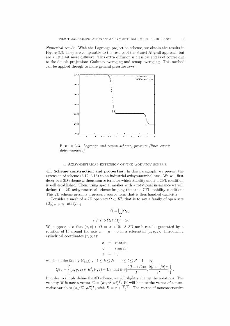
Numerical results. With the Lagrange-projection scheme, we obtain the results inFigure 3.3. They are comparable to the results of the Saurel-Abgrall approach butare a little bit more diffusive. This extra diffusion is classical and is of course dueto the double projection: Godunov averaging and remap averaging. This methodcan be applied though to more general pressure laws.

Figure 3.3. Lagrange and remap scheme, pressure (line: exact;dots: numeric)

4. Axisymmetrical extension of the Godunov scheme

4.1. Scheme construction and properties. In this paragraph, we present theextension of scheme (3.12, 3.13) to an industrial axisymmetrical case. We will firstdescribe a 3D scheme without source term for which stability under a CFL conditionis well established. Then, using special meshes with a rotational invariance we willdeduce the 2D axisymmetrical scheme keeping the same CFL stability condition.This 2D scheme presents a pressure source term that is thus handled explicitly.

Consider a mesh of a 2D open set Ω ⊂ R2, that is to say a family of open sets(Ωk)1≤k≤N satisfying

Ω =⋃

k

Ωk,

i 6= j ⇒ Ωi ∩ Ωj = ⊘.

We suppose also that (x, z) ∈ Ω ⇒ x > 0. A 3D mesh can be generated by arotation of Ω around the axis x = y = 0 in a referential (x, y, z). Introducingcylindrical coordinates (r, φ, z):

x = r cos φ,

y = r sin φ,

z = z,

we define the family (Qk,l) , 1 ≤ k ≤ N , 0 ≤ l ≤ P − 1 by

Qk,l =

(x, y, z) ∈ R3, (r, z) ∈ Ωk and φ ∈]

2(l − 1/2)π

P,2(l + 1/2)π

P[

.

In order to simply define the 3D scheme, we will slightly change the notations. Thevelocity −→u is now a vector −→u = (u1, u2, u3)T . W will be now the vector of conser-

vative variables (ρ, ρ−→u , ρE)T , with E = ε +−→u ·−→u

2 . The vector of nonconservative


variables is denoted by Y = (α, β)T with

(4.1) α =1

γ − 1, β =

γπ

γ − 1.

We define also a mixed vector as V = (W,Y )T .In 3D, the Euler equations read (Id is the identity matrix of size d × d)

ρt + ∇ · (ρ−→u ) = 0,

(ρ−→u )t + ∇ · (ρ−→u ⊗−→u + pI3) = 0,

(ρE)t + ∇ · ((ρE + p)−→u ) = 0.

Introducing the three fluxes:

G1(W ) = (ρu1, ρu1u1 + p, ρu1u2, ρu1u3, (ρE + p)u1),

G2(W ) = (ρu2, ρu2u1, ρu2u2 + p, ρu2u3, (ρE + p)u2),

G3(W ) = (ρu3, ρu3u1, ρu3u2, ρu3u3 + p, (ρE + p)u3),

and the vector flux G = (G1, G2, G3)T , the conservative equations can also bewritten

Wt + ∇ · G(W ) = 0.

Whereas for the nonconservative variables α and β, the equations are

Yt + −→u · ∇Y = 0,

and the pressure law is still the stiffened gas law which becomes

(4.2) p =1

αρε −

β

α.

Now, a 3D scheme reads∫

Qk,l

V n+1k,l − V n

k,l + τ

∫

∂Qk,l

F (V nk,l, V

nk′,l′ , ν) = 0,

where V nk,l is the approximation of V in Ωk,l at time tn, ν is the outward normal

vector to Qk,l on ∂Qk,l and Qk′,l′ denotes the neighbors of Qk,l along its boundary.The quantity F (·, ·, ν) is the numerical flux that we will now precisely define. Thedefinition of the numerical flux is based on the rotational invariance of the Eulerequations. This is very classical (see [13]). The only originality is the specialtreatment of the nonconservative variables.

First, a unit vector ν = (ν1, ν2, ν3)T is given. ν can also be written as ν =(cos φ sin θ, sin φ sin θ, cos θ). We define then the rotation matrix

M(ν) =

cos(φ) sin(θ) sin(φ) sin(θ) cos(θ)− sin(φ) cos(φ) 0

− cos(φ) cos(θ) − sin(φ) cos(θ) sin(θ)

,

which satisfies M(ν)ν = (1, 0, 0)T , and

N(ν) =

1 0M(ν)

0 I3

.

Consider now two states Va and Vb. In order to compute F (Va, Vb, ν), severalsteps are performed:

(1) Two rotated states are defined by Va = M(ν)Va and Vb = M(ν)Vb.


(2) The following augmented Riemann problem in the normal direction is thensolved

Wt + G1(W )x = 0,

Yt + u1Yx = 0,

V (0, x) =

Va if x < 0,

Vb if x > 0,

and the solution of this Riemann problem at x/t = 0 is denoted by V ∗.

(3) An interface state is recovered by the inverse rotation V ∗ = M(ν)−1V ∗.(4) The numerical flux is then set to

(4.3) F (Va, Vb, ν) = (G(W ∗) · ν, min(u∗ · ν, 0)(Y ∗b − Y ∗

a ))T .

It must be noted that this numerical flux is nonconservative on the Y vari-ables, as in the Saurel-Abgrall scheme that we presented in 1D cases. It canbe proved, as in the 1D case, that the resulting scheme preserves constantpressure and velocity states.

In our case the scheme will reduce to a 2D one thanks to several simplifications.First, thanks to the rotation matrix J (φ) = N(cos φ,− sinφ, 0) the axisymmetry

condition reads

V nk,l′ = J(

2(l′ − l)π

P)V n

k,l .

Thus, the velocity vector can be written −→u k,l = (uk cos( 2lπP ), uk sin( 2lπ

P ), vk)T andthe other variables do not depend on l. In this way, the scheme has only to bewritten on the cells Qk,0:

∫

Qk,0

(V n+1k,0 − V n

k,0) + τ

∫

∂Qk,0

F (V nk,0, J

(2l′π

P

)V n

k′,0, ν) = 0.

Denoting Vk,0 by Vk, this scheme then becomes∫

Ωk

(V n+1k − V n

k )rdr dz + τ

∫

∂Ωk

F (V nk , V n

k′ , ν)rdσ+

τP

2π

(∫

Ωk

F (V nk,0, J

(2π

P

)V n

k,0, ν)rdr dz +

∫

Ωk

F (V nk,0, J

(−2π

P

)V n

k,0, ν)rdr

)= 0.

It is then natural to let P tend to ∞. In the Riemann problems of the two lastintegrals only symmetric rarefaction waves occur. Thus those two terms reduce toa pressure term

(4.4)

∫

Ωk

(V n+1k −V n

k )rdr+τ

∫

∂Ωk

F (V nk , V n

k′ , ν)rdσ−τ

∫

Ωk

(0, pnk , 0 · · · 0)T rdr = 0.

We recover, of course, an approximation of the axisymmetrical equations, namely

(ρr)t + (ρur)x + (ρvr)z = 0,

(ρur)t + (ρu2r + pr)x + (ρuvr)z = pr,

(ρur)t + (ρvur)x + (ρv2r + pr)z = 0,

(ρEr)t + ((ρE + p)ur)x + ((ρE + p)vr)z = 0,

αt + uαx + vαz = 0,

βt + uβx + vβz = 0.

One advantage of this approach is that the pressure source term can be hand-led explicitly without modifying the 3D CFL condition. We have also avoidedaxisymmetrical source terms which are singular on the axis of rotation. Finally, theresulting scheme preserves constant pressure and velocity states. The construction


of a 2D scheme that preserves contact discontinuities with discontinuous tangentialvelocity is proposed in Nkonga [5].

4.2. Boundary conditions. For a boundary cell Ωk, an artificial value V nk′ has to

be defined for the part of ∂Ωk that meets the boundary. For simplicity, supposethat the normal vector is ν = (1, 0). We index by (i) (as“inside”) the components ofV n

k and by (o) (as “outside”) the (unknown) components of V nk′ . Several boundary

conditions can then be used:

• “Supersonic” inlet:

Vo = given state.

• “Supersonic” outlet:

Vo = Vi.

• Pressure imposed (“subsonic” outlet). The outside state with pressure po islinked to the inside state by a one-wave (shock or rarefaction). With thenotations of §7.2, we find

ρo = 1/Hi(po),

uo = ui − Xi(po),

vo = vi,

αo = αi,

βo = βi.

• Pressure and density imposed (“subsonic” inlet). Pressure po and density ρo

of the outside state are given. The nature of the outside state (αo, βo) andthe tangential velocity (vo) are also supposed to be known. Here, the outsidestate is linked to the inside state by a one-wave (shock or rarefaction) anda contact discontinuity. This permits to compute the unknown normalvelocity

uo = ui − Xi(po).

• Mirror state. This boundary condition is used at a solid boundary. Allthe components of the state Wo are the same as those of state Wi but thenormal velocity

uo = −ui.

It is important here to point out that the terminology“subsonic”or“supersonic”hasnothing to do with the true nature of the flow at the boundary. It is only linked towhat is expected when Wo ≃ Wi. Indeed, we can imagine imposing a “supersonic”inlet boundary condition and observing, at this boundary a supersonic outflow! Theresolution of a Riemann problem ensures that the redundant information will beforgotten, if necessary. For more details about this technique, we refer to Duboisand his theory of partial Riemann problems [8].

4.3. Optimisation of the CFL number. An important constraint in any finitevolumes scheme is the Courant-Friedrichs-Lewy condition. It expresses that, forany finite volume Ωk the time step τ must verify

(4.5) τ <surf(Ωk)

length(∂Ωk)V ∗,

where V ∗ is the maximal wave speed in the solution of all the Riemann problemsat the cell interfaces. For a classical Godunov scheme on an unstructured mesh, itis proved in [6], that the CFL condition (4.5) implies the positivity of the scheme(the density remains >0) and the fact that it is entropic for any Lax entropy. Weassume that this is still true for the Saurel-Abgrall scheme. In the case wherelarge and small cells are mixed, the CFL condition on the small cells imposes the


global CFL condition. The mixing of large and small cells can be imposed by thegeometry (an example is given below) and not necessarily by a required precisionof the computation. In order to reduce the computational cost it is possible touse several time steps, a small one for the small cells and a bigger one for the bigcells. Then, several time steps are performed on the small cells and less time stepsare performed on the big cells. The time reduction of the computation can besignificant.

The time marching algorithm can be formalized as follow.First, in a initialization procedure, an ideal time step is computed for each cell

Ωk. Let δ be the desired CFL number (for example δ = 0.7). The local time stepis defined by

(4.6) τk = δsurf(Ωk)

length(∂Ωk)V ∗.

The maximal time step in the mesh is noted τmax. In the same way, the minimaltime step is τmin. Let n0 be the smallest integer such that 2n0+1τmin > τmax Wewill then say that the cell Ωk has a CFL level of j if

(4.7) 2j−1τmin ≤ τk < 2jτmin.

Thus a CFL level of 1 corresponds to the smallest cells and a CFL level of n0

corresponds to the biggest cells. We define also a CFL level for the edges. An edgeEl has a CFL level which is the smallest CFL level of its two neighboring cells. Inorder to advance by a global time step 2n0τmin, the algorithm is:

• for all integer j = 1 . . . n0 do– for all edges of CFL level ≤ j do

∗ compute the flux∗ distribute it to the two neighboring cells

– enddo– update only the cells of level ≤ j

• enddo

In this way, the scheme remains conservative and stable. The gain in computationtime is of order 2n0 if the number of small cells is small.

5. An industrial application

5.1. Description. The industrial system that we wish to simulate is a gas gen-erator whose geometry and working order are indicated in Figure 5.1. The gasgenerator is made of a combustion chamber (top), a cooling chamber (middle part)and an evacuation pipe (bottom, not represented). Only the working order in thecooling chamber will be numerically simulated.

The cooling chamber and the evacuation pipe are separated by a metallic mem-brane. This membrane can withstand a pressure of 40 bar. The cooling chamberis around 1 m high, it is itself split into several chambers: a central one and a se-condary one which communicate through an intermediate chamber and two seriesof holes.

At time t = 0 ms, the cooling chamber is filled with motionless air and waterat a pressure of 5 bar. Gas at high pressure (∼ 100 bar) and high temperature(∼ 2500 K) are then produced in the combustion chamber. They rush into thecooling chamber and impact on the water surface causing a shock wave to propagatein the water. When it reaches the bottom membrane, it smashes it. A part of thewater is then drained in the evacuation pipe, the rest of the water is transferredinto the secondary chamber where it is finally re-injected through very small holesin the draining pipe and mixed with the gas still rushing from the combustionchamber. The entire process, from the beginning of combustion to the beginning


of the liquid re-injection has an approximate duration of 50 ms. This justifies thefact that we neglect vaporization. Of course, for longer simulations, vaporizationshould be taken into account.

As one can note in Figure 5.1, the real geometry of the cooling chamber is notaxisymmetrical due to the presence of re-injection holes near the draining pipe andconnection holes between the several chambers. For the simulation we thus replacethese holes by slits of equivalent area. The simplified axisymmetrical geometry isrepresented in Figure 5.2. Here we plot the density. Red corresponds to densityvalues of the liquid (∼ 1000 kg/m3) whereas black corresponds to density values ofthe gas (∼ 10 kg/m3).

5.2. Results. A part of the mesh is represented in Figure 5.3. It appears that verysmall cells are necessary in the injection slits. The CFL stability condition is thusvery restrictive on these cells. In order to avoid a overly long computation we usethe algorithm described in §4.3. With this technique it is possible to perform a 50ms simulation in 5 hours CPU on an 1.4 GHz computer. It should be noted thatthe exact Riemann solver requires at most 5 Newton iterations for convergence towithin 10−10p0 where p0 is the atmospheric pressure. Most of the zones in the fluidflow do not require as many iterations - 2 or 3 only. In conclusion, the classicalGodunov scheme is not as expensive as is so often proclaimed in the literature.

We then run the scheme presented in §4.1 and §4.2. Gravity is neglected. Theboundary conditions and initial conditions are depicted in Figure 5.2. The boundaryconditions are imposed according to the technique described in §4.2:

• At the top entrance of the cooling chamber, which corresponds to the exitof the combustion chamber, we impose pressure p(t) and density ρ(t). Thetime evolution of these quantities is determined by experimental measure-ments. The pressure increases from 10 to 120 bar in several milliseconds.We observe that the speed increases from 10 to 700 m/s. The flow thusremains subsonic.

• At the bottom exit, the boundary condition is, at first, a solid wall con-dition. When the pressure reaches 40 bar (this occurs around 6 ms), theboundary condition is changed into an outflow condition. We then imposean outside pressure of 5 bar. The pressure then drops progressively from40 to 5 bar, and the velocity increases from 0 to 1500 m/s. The flow is thussupersonic at the end of the computation.

Then, in Figures 5.4, 5.5 and 5.6 iso-densities for several instants are plotted. Wecan point out the following:

• At 10 ms, the gas begins to push the water. The free surface is slightlydeformed. We observe a smoothing of the density profiles due to the nu-merical diffusion of the interface. But despite the first order scheme (andthanks to a quite fine mesh..)., the interface is easily recognized.

• The instant 15 ms is after the bursting of the membrane. We can see thatthe central part of the water in the cooling chamber has been drained intothe evacuation pipe.

• At instants 20 ms and 25 ms, water has already entered the secondarychamber, forming a jet against its boundary. The jet is numerically diffusedbut still visible.

• At instant 50 ms, the jet has impacted on the free surface in the secondarychamber. We observe that the re-injection has started (small jet at thebottom).


Figure 5.1. Gas generator

(a) gas-generator (start) (b) gas-generator(middle)

(c) gas-generator (end)

• In Figure 5.4, we plot pressure in order to demonstrate the appearance ofnegative values of the pressure. These negative values appear in the bottomnozzle where a strong drop of pressure is probably triggering cavitation.

Measurements on a real gas generator were performed at the “Direction des Con-structions Navales” (DCN) in Toulon (France). Excellent agreement is observedin the central part of the cooling chamber. For example, the bursting time of theseparating membrane is predicted with an error of a few percent. More precise com-parisons with experiments have now to be performed in the secondary chambers.

6. Conclusion

In this paper we have first recalled basic facts on compressible multifluid flows.We have also carefully described the spurious pressure oscillations phenomenon thatarises in any conservative Godunov scheme applied to multifluid flows.

We focused on two remedies to suppress these oscillations. The first fix has beenproposed by Saurel and Abgrall in [24]. It is based on a nonconservative transportof the pressure law coefficients and works only for a stiffened gas pressure law. Thesecond fix is, to our knowledge, new and is based on a Lagrange plus projectionscheme. In the projection step we project the pressure instead of the pressure lawcoefficients. The resulting scheme is more diffusive than the Saurel-Abgrall schemebut also more general (it works for any pressure law).

Because in our application the stiffened gas law is sufficient we decided to exploitthe Saurel-Abgrall scheme in a 2D axisymmetrical and complex geometry. Wehad then to deal with some practical problems: negative pressures, axisymmetry,unstructured meshes, boundary conditions, multi time steps.


Figure 5.2. Boundaries

(a) axisymmetrical geometry and bound-aries

Figure 5.3. Mesh

(a) Mesh (partial view)

After having solved these problems, we were in a situation to present a usefulindustrial numerical simulation.

Future studies could now follow several directions:


Figure 5.4. Cavitation

(a) density (kg/m3) at 10 ms

(b) pressure (bar) at 10 ms


Figure 5.5. Density plots (kg/m3)

(a) density at 15 ms

(b) density at 20 ms


Figure 5.6. Density plots (kg/m3)

(a) density at 25 ms

(b) density at 50 ms


• The scheme should be extended to second order. We have not done itbecause in axisymmetrical cases, the classical second order extensions (asthe MUSCL method of Van Leer [26]) are surprisingly not straightforward.

• The second important aspect is to be able to deal with true cavitation, i.e.the vaporization of the liquid in a metastable state. Some progress has beenobtained in the case of a liquid-vapor flow in [16]. The case of the three-phase flow with air, liquid and vapor is being studied. Some preliminaryresults can be found in [4].

7. Appendix

7.1. Entropy and hyperbolicity. We study here the hyperbolicity of (2.9), (2.1).For this purpose, it is classical to introduce the specific entropy

s0 =p + π

ργ= s0(W ).

A simple computation shows that if W is a regular solution of (2.1), (2.9), then s0

satisfies the advection equation

s0t + us0

x = 0.

Thus, for any function g of s0, γ and π an additional conservation law is satisfiedby ρg(s0, γ, π)

(ρg(s0, γ, π))t + (ρug(s0, γ, π))x = 0.

If W → S(W ) = ρg(s0, γ, π) is convex, we get in this way all the Lax entropiesof system (2.9), (2.1). For a proof of this result, we refer to the review paperof [15]. According to Mock’s theorem [21] the convexity of S would then implyhyperbolicity. Here, we prefer to carry out a more direct calculation. Always forregular solutions, we set

Y =

ρus0

γπ

.

We then have

Yt + B(Y )Yx = 0,

with

B(Y ) =

u ρ 0 0 0

γ p+πρ2 u ργ−1 (p+π) ln(ρ)

ρ − 1ρ

0 0 u 0 00 0 0 u 00 0 0 0 u

.

The eigenvalues of B are (u − c, u, u, u, u + c) with c2 = γ p+πρ . Thus, if ρ > 0, the

system is hyperbolic if and only if

p + π ≥ 0.

Remark 7.1. When p tends to −π keeping the specific entropy constant, which isthe case in a rarefaction wave, we get:

ρ = C (p + π)1/γ

→ 0.

Thus, the limiting case p = −π corresponds to a zero density ρ = 0. This meansthat, in a liquid, vacuum corresponds to a negative value of the pressure.


7.2. Global resolution of the Riemann problem. As in the case of gas dy-namics for one fluid, the fields 1 and 3, which correspond to the eigenvalues u − cand u+c are genuinely non-linear whereas the field 2 corresponding to the multipleeigenvalue u is linearly degenerate (contact discontinuity).

At present, we have written several forms (conservative or not) for the convectionequations. All these forms are formally equivalent. It is important to verify thatthey are correct also for discontinuous solutions.

Let us consider a discontinuity propagating with velocity σ. Indexes (a) and (b)will be relative to the two sides of the discontinuity. Rankine-Hugoniot relationsread, in this case

σ(Wa − Wb) = F (Wa) − F (Wb).

Introducing the relative velocity to the discontinuity and the specific volume

v = u − σ, τ =1

ρ,

the jump relations become

M = ρava = ρbvb,

ρav2a + pa = ρbv

2b + pb,

(ρa(εa +v2

a

2+ pa)va = (ρb(εb +

v2b

2) + pb)vb,

Mγa = Mγb,

Mπa = Mπb.

The last two relations implie that γ and π can jump only at the contact discon-tinuity (when M = 0). On the other hand, a simple computation shows that γ andπ are Riemann invariants for the fields 1 and 3.

Remark 7.2. These two properties imply that in genuinely non-linear fields the co-efficients γ and π are constant. Outside the contact discontinuity, the computationsare thus identical to the case of a single fluid. These classical computations canbe found for example in the book of Godlewski and Raviart [13]. They are brieflysketched below.

Remark 7.3. We have also given a sense to the nonconservative products in thelast two transport equations in (2.16) because u and the pressure law coefficientscannot present a simultaneous jump.

Solving the Riemann problem means finding the weak entropy solution of

Wt + F (W )x = 0,

W (0, x) =

Wl if x < 0,Wr if x > 0.

This solution is supposed to be self-similar

W (t, x) = R(x

t,Wl,Wr

).

It is made up of constant states separated by shock waves, rarefaction waves or acontact discontinuity. It is thus of the form

R(ξ,Wl,Wr) =

Wl if ξ < λ−1 ,

WI if λ+1 < ξ < λ2,

WII if λ2 < ξ < λ−3 ,

Wr if λ+3 < ξ,

where the unknowns are WI , WII and the velocities λ2, λ±i , i = 1, 3 which satisfy

λ−1 ≤ λ+

1 < λ2 < λ−3 ≤ λ+

3 .


Furthermore, if λ−i < λ+

i (resp. if λ−i = λ+

i ) then the i-wave is a rarefactionwave (resp. a shock of velocity σ = λ−

i = λ+i ). When the i-wave is a rarefaction,

the computation of W = R(ξ, Wl, Wr) , for λ−i < ξ < λ+

i is classically carried outby expressing that the three Riemann invariants are constant in the i-rarefaction(see [13]).

On the other hand, we have pI = pII = p⋆. If no vacuum occurs, we can alsowrite uI = uII = u⋆. Moreover, from remark 7.2, we have that γI = γl, γII = γr,πI = πl, πII = πr. It is then classical to compute the 1- and 3-waves from thepressure p⋆ common to the two intermediate states WI et WII . For this purpose,we introduce the functions

ha(p⋆) = τa(γa + 1)(pa + πa) + (γa − 1)(p⋆ + πa)

(γa + 1)(p⋆ + πa) + (γa − 1)(pa + πa), a = l or r,

Φa(p⋆) =√

(p⋆ − pa)(τa − ha(p⋆)),

ga(p⋆) = τa

(pa + πa

p⋆ + πa

)1/γa

,

Ψa(p⋆) =2

γa − 1(τaγa(pa + πa))1/2

((p⋆ + πa

pa + πa)

γa−1

2γa − 1

),

Xa(p⋆) =

Φa(p⋆) if p⋆ > pa,Ψa(p⋆) if p⋆ < pa,

Ha(p⋆) =

ha(p⋆) if p⋆ > pa,ga(p⋆) if p⋆ < pa.

We thus get

uI = ul − Xl(p⋆),

uII = ur + Xr(p⋆),

τI = Hl(p⋆),

τII = Hr(p⋆),

and the Riemann problem is solved when p⋆ is known.If no vacuum region appears, the following theorem holds.

Theorem 7.4. Let p0 = min(πl, πr). If

(7.1) ur − ul ≤ − (Xl(−p0) + Xr(−p0)) ,

then the Riemann problem has a unique solution. The pressure p⋆ ≥ −p0 is theunique solution of

ul − Xl(p⋆) = ur + Xr(p

⋆).

This result is quite similar to the case of the Riemann problem for a single fluid.For the proof we refer (for example) to [14], [13].

When inequality (7.1) is not true, a vacuum has to be introduced. This vacuumregion appears in the fluid whose coefficient π is the smallest.

Theorem 7.5. If

ur − ul > − (Xl(−p0) + Xr(−p0)) ,

the Riemann problem has still an entropy solution. For example, if p0 = πl, thenwe have p⋆ = −p0, ρI = 0, u⋆ = uII = ur + Xr(p

⋆). uI = ul − Xl(p⋆), and, in

general uI 6= uII .


Proof. Suppose that p0 = min(πl, πr) = πl. In the two open sets x < u⋆t andx > u⋆t, the computation of the 1- and 3-wave curves is identical to the mono-fluid case. Thus, W (t, x) is indeed an entropy solution of the Riemann problem inthese two open sets. It is then sufficient to verify that, at the contact discontinuityx/t = u⋆, Rankine-Hugoniot jump relations are satisfied, together with the entropycondition. The discontinuity velocity is σ = u⋆. We thus have vII = u⋆ − σ = 0.Mass conservation ρIvI = 0 = ρIIvII is then satisfied. In the same way, ρIv

2I +p⋆ =

p⋆ = ρIIv2II + p⋆. The jump relation for the conservation of ρϕ is also satisfied:

ρIvIϕI = 0 = ρIIvIIϕII . For the energy jump relation, we use the fact that the 1-wave is necessarily a rarefaction because p⋆ = −p0 ≤ pl. However, in a rarefaction,

when p → −π, then ρε+π → 0 (see remark 7.1) and we have (ρIεI +p⋆)vI +ρIv3

I

2 =

0 = (ρIIεII + p⋆)vII + ρIIv3

II

2 . Finally, the entropy inequality (which degeneratesto an equality) is also satisfied: ρIvIsI = 0 = ρIIvIIsII . ¤

References

[1] R. Abgrall. Generalisation of the roe scheme for the computation of mixture of perfect gases.Recherche Aerospatiale, 6:31–43, 1988.

[2] R. Abgrall. How to prevent pressure oscillations in multicomponent flow calculations: a quasi-conservative approach. J. Comput. Phys., 125(1):150–160, 1996.

[3] R. Abgrall and S. Karni. Computations of compressible multifluids. Journal of ComputationalPhysics, 169(2):594–623, 2001.

[4] T. Barberon. Modelisation mathematique et numerique de la cavitation dans les ecoulementsmultiphasiques compressibles. PhD thesis, Universite de Toulon, 2002.

[5] C. Berthon and B. Nkonga. Behavior of the finite volumes schemes in material and numericalinterfaces. In Finite Volumes for Complex Applications III (Porquerolles, 2002), pages 139–146. Hermes Penton Ltd, London, 2002.

[6] A. Chalabi and J.-P. Vila. Operator splitting, fractional steps method and entropy condition.In Third International Conference on Hyperbolic Problems, Vol. I, II (Uppsala, 1990), pages226–240. Studentlitteratur, Lund, 1991.

[7] J. P. Cocchi and R. Saurel. A Riemann problem based method for the resolution of compress-ible multimaterial flows. Journal of Computational Physics, 137(2):265–298, 1997.

[8] F. Dubois. Partial riemann problem, boundary conditions and gas dynamics. In AbsorbingBoundaries and Layers, Domain Decomposition Methods. Applications to Large Scale Com-putations, Loıc Tourrette and Laurence Halpern, eds., pages 16–77. Nova Science Publishers,Inc., New York, 2001.

[9] F. Dubois and P. LeFloch. Boundary conditions for nonlinear hyperbolic systems of conser-vation laws. J. Differential Equations, 71(1):93–122, 1988.

[10] R. P. Fedkiw, T. Aslam, B. Merriman, and S. Osher. A non-oscillatory Eulerian approach tointerfaces in multimaterial flows (the ghost fluid method). J. Comput. Phys., 152(2):457–492,1999.

[11] J. P. Franc and al. La Cavitation: Mecanismes Physiques et Aspects Industriels. PressesUniversitaires de Grenoble, 1995.

[12] T. Gallouet, J. M. Herard, and Seguin N. A hybrid scheme to compute contact discontinuitiesin one-dimensional euler systems. M2AN, 36(6):1133–1159, 2003.

[13] E. Godlewski and P. A. Raviart. Numerical approximation of hyperbolic systems of conser-vation laws. Springer, 1996.

[14] S. Godounov, A. Zabrodine, M. Ivanov, A. Kraıko, and G. Prokopov. Resolution numeriquedes problemes multidimensionnels de la dynamique des gaz. “Mir”, Moscow, 1979. Translatedfrom the Russian by Valeri Platonov.

[15] A. Harten, P. D. Lax, C. D. Levermore, and W. J. Morokoff. Convex entropies and hyper-bolicity for general Euler equations. SIAM J. Numer. Anal., 35(6):2117–2127, 1998.

[16] P. Helluy and T. Barberon. Finite volume simulations of cavitating flows. In Finite Volumesfor Complex Applications III (Porquerolles, 2002), pages 455–462. Hermes Penton Ltd, Lon-don, 2002.

[17] T. Y. Hou and P. G. LeFloch. Why nonconservative schemes converge to wrong solutions:error analysis. Math. Comp., 62(206):497–530, 1994.

[18] S. Karni. Multicomponent flow calculations by a consistent primitive algorithm. Journal ofComputational Physics, n 47:1115–1145, 1994.

[19] S. Karni. Hybrid multifluid algorithms. SIAM J. Sci. Comput., 17(5):1019–1039, 1996.


[20] P. Kuszla and V. Daru. Numerical simulation of high-speed liquid jets. In Computationalmechanics (Buenos Aires, 1998). Centro Internac. Metodos Numer. Ing., Barcelona, 1998.

[21] M. S. Mock. Systems of conservation laws of mixed type. J. Differential Equations, 37(1):70–88, 1980.

[22] W. Mulder, S. Osher, and J. A. Sethian. Computing interface motion in compressible gasdynamics. J. Comput. Phys., 100(2):209–228, 1992.

[23] S. Rouy. Modelisation mathematique et numerique d’ecoulements diphasiques compressibles.PhD thesis, Universite de Toulon, December 2000.

[24] R. Saurel and R. Abgrall. A simple method for compressible multifluid flows. SIAM J. Sci.Comput., 21(3):1115–1145, 1999.

[25] R. Saurel, J.P. Cocchi, and P.B. Butler. A numerical study of cavitation in the wake of ahypervelocity underwater projectile. AIAA Journal of Propulsion and Power, 15(4):513–522,1999.

[26] B. Van Leer. Towards the ultimate conservative difference scheme. a second order sequel tothe godunov’s method. Journal of Computational Physics, 32:101–136, 1979.

practical computation of axisymmetrical multifluid flows

Documents