practical applications of laser absorption spectroscopy for aeroengine testing...
TRANSCRIPT

PRACTICAL APPLICATIONS OF LASER ABSORPTION
SPECTROSCOPY FOR AEROENGINE TESTING
A DISSERTATION
SUBMITTED TO THE DEPARTMENT OF MECHANICAL
ENGINEERING
AND THE COMMITTEE ON GRADUATE STUDIES
OF STANFORD UNIVERSITY
IN PARTIAL FULFILLMENT OF THE REQUIREMENTS
FOR THE DEGREE OF
DOCTOR OF PHILOSOPHY
Ian Schultz
June 2014

http://creativecommons.org/licenses/by-nc/3.0/us/
This dissertation is online at: http://purl.stanford.edu/rb827vr6771
© 2014 by Ian Alexander Schultz. All Rights Reserved.
Re-distributed by Stanford University under license with the author.
This work is licensed under a Creative Commons Attribution-Noncommercial 3.0 United States License.
ii

I certify that I have read this dissertation and that, in my opinion, it is fully adequatein scope and quality as a dissertation for the degree of Doctor of Philosophy.
Ronald Hanson, Primary Adviser
I certify that I have read this dissertation and that, in my opinion, it is fully adequatein scope and quality as a dissertation for the degree of Doctor of Philosophy.
David Davidson
I certify that I have read this dissertation and that, in my opinion, it is fully adequatein scope and quality as a dissertation for the degree of Doctor of Philosophy.
Reginald Mitchell
Approved for the Stanford University Committee on Graduate Studies.
Patricia J. Gumport, Vice Provost for Graduate Education
This signature page was generated electronically upon submission of this dissertation in electronic format. An original signed hard copy of the signature page is on file inUniversity Archives.
iii

iv

Abstract
Reliable air-breathing hypersonic propulsion systems offer the potential to revolu-
tionize aircraft performance in a variety of high-speed aerospace applications through
substantial efficiency gains and hardware cost savings. Supersonic combustion ram-
jet (scramjet) engines are one such device that promise propulsion capabilities up to
about Mach 10. At these speeds, a flight from San Francisco to Paris would take
around an hour. However, before these devices are ever practically realized, consid-
erable technical challenges must be overcome in combustor-inlet interaction, fuel-air
mixing, and coupled turbulent flow/combustion modeling. The growing power of com-
putational tools have accelerated the pace of solving these problems, but the accuracy
of computational approaches can only be validated by rigorous experimental testing.
Thus, there is a need for both facilities capable of creating conditions experienced
during hypersonic flight, as well as diagnostics that can characterize the operation
of those facilities and provide experimental data for the validation of computational
models.
Optical diagnostics such as laser absorption spectroscopy are capable of providing
non-intrusive, in situ measurements of important flow-field parameters such as tem-
perature, velocity, species concentrations, which makes them an invaluable resource
to hypersonic aeroengine researchers. Absorption spectroscopy, in particular, has
benefited from recent advances in laser and optics technology, allowing access to a va-
riety of wavelengths corresponding to absorption transitions of important combustion
species such as O2, H2O, and CO2. Moreover, these sensors only require compact,
low-power laser sources and light can be delivered via fiber-optics, which enables the
v

sensor to more easily integrate with test facility hardware. As a result, laser absorp-
tion spectroscopy has become a workhorse in experimental scramjet research, and has
been applied in test facilities around the world.
Building upon this prior work, here the design and results of several different spec-
troscopic sensors for facility characterization and distinct scramjet operation modes
are presented. Both hydrogen-fueled and hydrocarbon-fueled scramjets are investi-
gated in a variety of geometric configurations. These results comprise the largest
data set of laser absorption spectroscopy measurements within scramjet combustors
published to date, and are a valuable resource for computational researchers who wish
to compare their models with experimental data. A primary drawback of laser ab-
sorption spectroscopy is that some techniques are sensitive to nonuniformity along the
measurement line-of-sight. In highly three-dimensional flows such as within a scramjet
combustor, this can prove to be a considerable hindrance. However, in the work here
particular care has been taken to account for nonuniformity along the measurement
path, and new techniques, including a new approach to wavelength-modulation spec-
troscopy data reduction, have been developed and applied to provide quantitatively
accurate path-integrated measurements in the presence of nonuniformities. Addition-
ally, novel applications of laser absorption spectroscopy are presented, including the
use of absorption data to place an upper bound on the cavity residence time within
a scramjet combustor, and a new sensor design for measuring air temperature in
high-enthalpy facilities by tracking the formation of nitric oxide.
Results include two-dimension spatially-resolved measurements of temperature,
H2O concentration, and velocity downstream of fuel injection in a hydrogen-fueled
Mach 5 scramjet combustor, which reveal combustion progress through the develop-
ment of a high-temperature, water-rich product plume. Measurements are compared
to computational fluid dynamics (CFD) simulations, which reveal some inaccuracies
in the CFD, including a general over-prediction of combustion progress. Additional
tests in a Mach 10 scramjet combustor for measurements of temperature and H2O
concentration downstream of fuel injection identify the presence of driver-gas con-
tamination during the test time in a non-combusting case, and ignition onset during
hydrogen-air combustion experiments. CFD comparisons yield similar results to Mach
vi

5 testing: there is reasonable agreement between measurements and simulations, but
there is a general over-prediction of extent of combustion by the CFD. The application
of mid-infrared laser absorption sensors for detection of temperature, H2O, CO, and
CO2 concentration in an ethylene-fueled Mach 5 scramjet is also discussed. Results
from field measurements reveal combustion progress with axial progression, however
a large concentrations of the combustion intermediate species CO indicates incom-
plete combustion. Temporal variation in measurements are analyzed and attributed
to unsteady shear-layer interactions in the cavity-flameholder combustor geometry.
Finally, the design, development, and laboratory validation of a mid-infrared nitric
oxide sensor for measuring air temperature at high-temperatures and -pressures is
presented.
This work leverages recent advances in laser hardware and spectroscopic data
processing technology to present a suite of laser absorption diagnostic tools for char-
acterizing performance in aeroengine test environments. The results demonstrate the
usefulness of these sensors for investigating the many competing physical processes
in these complex devices. Moreover, these measurements provide a feedback mecha-
nism for CFD modelers who wish to validate simulation performance, and the sensors
described here can be integrated into other scramjet combustion facilities where the
simplicity and diagnostic power of laser absorption spectroscopy is desirable.
vii

Acknowledgments
Throughout my academic career, I have been exceptionally fortunate to enjoy sup-
port from a wide array of family, friends, mentors, and colleagues who have made my
graduate studies possible. Going all the way back to grade school, I remember all the
encouragement from my teachers to pursue math and science as career possibilities.
Without that early support, I am not sure I would be writing this today. In my un-
dergraduate days at UCLA, Professor Ann Karagozian was always available to discuss
research or life in general, and encouraged me to pursue a Ph.D. at Stanford. My first
taste of research was at UCLA as an undergraduate research assistant with Sophonias
Teshome, then a graduate student. His patience and effort was an important part of
motivating me to advance my career as a scientist. Finally, my roommate through
three years of undergraduate work was James Umali, whose mastery of engineering
coursework pushed me to excel, even if I had to settle for second-best.
Stanford is a particularly special place and I have been lucky to spend five years
of my life studying here. The combination of motivated colleagues, excellent mentors,
and stimulating classes cannot be beat. I owe a debt of gratitude to Professor Hanson,
who took a chance on me straight out of my undergraduate studies and hired me as
a research assistant. He didn’t just teach me how to make spectroscopic sensors, but
more importantly, he showed me how far exacting standards and attention to detail
can take you in research and in life. Professor Hanson’s high expectations certainly
made life challenging at times, but ultimately the skills I have developed as a result
will allow me to succeed in any future endeavor. He truly is a world-class researcher
and I have been lucky to study under his tutelage.
Professor Hanson’s research group has been a pleasure to work in throughout my
viii

time at Stanford, largely due to the wonderful people that it consists of. Not only is
the atmosphere friendly and collegial, but there were nearly constant opportunities to
learn when surrounded by so many intelligent people. In particular, Dr. Jay Jeffries
worked tirelessly to make sure measurement campaigns at remote facilities could
be completed successfully. He has always been available for research advice and a
friendly conversation, and his knowledge of lasers and optics is unparalleled. Dr. Dave
Davidson truly is a shock-tube guru and has been an invaluable resource whenever
issues arose with shock-tube experiments. Chris Goldenstein was an excellent research
partner and travel companion for nearly every field campaign contained in this thesis
(and a few trips that aren’t even here!). His passion for developing new sensors
and techniques is admirable, and his depth of knowledge in wavelength modulation
spectroscopy was crucial to many of our successes. Thanks also to Mitchell Spearrin,
Christopher Strand, Ritobrata Sur, Matthew Campbell, Tom Parise, Yangye Zhu,
Leyen Chang, Brian Lam, Ivo Stranic, Vic Miller, and the rest of the Hanson Group
– I have had the good fortune to work with many great colleagues over the years, and
I will miss afternoon coffee and discussions of our research.
Most of all, though, I would like to thank my family. My parents, Brad and
Debbie, have always been there to help me with studies and provided me with a great
childhood environment where I had the luxury of spending my time doing homework
and playing instead of worrying about the real world. My sister Alene and brother
in-law Tony have constantly inspired me with their creative spirit and easy-going
attitude. My uncles, aunts, cousins and all of the Schultz family has always been
supportive. On my mother’s side, the life my grandparents Suzie and Rene (or Meme
and Papa as I have always called them) have made here in America after emigrating
from Switzerland always been inspirational, and their support has been unconditional.
One last person deserves special mention. Had I never come to Stanford, I would
have never met my girlfriend, Jennifer. She has patiently supported me through late
nights sitting behind the glow of the computer, interrupted movies to respond to
emails, Saturdays at home processing data, and all of the other less-desirable aspects
of being a graduate student. She has never questioned my resolve to finish what I
had started, and her love and support has made my graduate studies infinitely more
ix

enjoyable. I am deeply grateful for her presence in my life, and would like to thank
her for all that she has done.
x

Contents
Abstract v
Acknowledgments viii
1 Introduction and Motivation 1
1.1 Scramjet Engine Development . . . . . . . . . . . . . . . . . . . . . . 1
1.2 The Role of Absorption Spectroscopy . . . . . . . . . . . . . . . . . . 4
1.3 Overview of Thesis . . . . . . . . . . . . . . . . . . . . . . . . . . . . 5
2 Spectroscopic Theory 8
2.1 Introduction to Spectroscopic Theory . . . . . . . . . . . . . . . . . . 8
2.2 Direct-Absorption Spectroscopy . . . . . . . . . . . . . . . . . . . . . 9
2.3 Wavelength-Modulation Spectroscopy . . . . . . . . . . . . . . . . . . 14
2.3.1 WMS Model . . . . . . . . . . . . . . . . . . . . . . . . . . . . 15
2.3.2 Scanned-Wavelength-WMS-2f /1f . . . . . . . . . . . . . . . . 21
2.4 Velocimetry . . . . . . . . . . . . . . . . . . . . . . . . . . . . . . . . 23
2.5 Spectroscopic Sensing in Nonuniform Flows . . . . . . . . . . . . . . 24
2.5.1 In Situ Measurement of Collision Linewidth . . . . . . . . . . 27
2.5.2 Column Density as a Concentration Measurement . . . . . . . 28
2.5.3 Line Selection Principles for Nonuniform Flows . . . . . . . . 29
3 Measurements in a Continuous Flow, H2-Fueled Model Scramjet
Combustor 33
3.1 Sensor Architecture . . . . . . . . . . . . . . . . . . . . . . . . . . . . 35
xi

3.1.1 Scramjet Facility Description . . . . . . . . . . . . . . . . . . 35
3.1.2 Wavelength Selection and Spectroscopic Model . . . . . . . . . 37
3.1.3 TDLAS Sensor Description . . . . . . . . . . . . . . . . . . . . 39
3.2 Uncertainty Analysis of WMS Measurements . . . . . . . . . . . . . . 42
3.3 TDLAS Measurements: “Configuration A” . . . . . . . . . . . . . . . 44
3.3.1 Φ = 0.17 Equivalence Ratio Combustion Results . . . . . . . . 44
3.3.2 Comparisons of TDLAS Data with CFD Simulations . . . . . 46
3.4 TDLAS Measurements: “Configuration C” . . . . . . . . . . . . . . . 49
3.4.1 Steam Addition Measurements . . . . . . . . . . . . . . . . . . 49
3.4.2 Combustion Measurements . . . . . . . . . . . . . . . . . . . . 51
4 Multispecies Measurements in a Hydrocarbon-Fueled Scramjet Com-
bustor 58
4.1 Mid-IR Absorption Transition Selection . . . . . . . . . . . . . . . . . 60
4.2 Facility Description . . . . . . . . . . . . . . . . . . . . . . . . . . . . 63
4.3 Absorption Spectroscopy Sensor Hardware . . . . . . . . . . . . . . . 64
4.4 Results . . . . . . . . . . . . . . . . . . . . . . . . . . . . . . . . . . . 66
4.4.1 Multispecies Combustion Product Measurements . . . . . . . 66
4.4.2 Combustion Unsteadiness . . . . . . . . . . . . . . . . . . . . 70
4.4.3 Transient Measurements Within the Cavity During Flame Ex-
tinction . . . . . . . . . . . . . . . . . . . . . . . . . . . . . . 72
5 Hypersonic Scramjet Combustor Measurements Within a Reflected
Shock Tunnel 77
5.1 Hardware Description . . . . . . . . . . . . . . . . . . . . . . . . . . . 79
5.1.1 ATK HyPulse Test Facility . . . . . . . . . . . . . . . . . . . . 79
5.1.2 TDLAS Sensor Layout . . . . . . . . . . . . . . . . . . . . . . 80
5.2 Results . . . . . . . . . . . . . . . . . . . . . . . . . . . . . . . . . . . 83
5.2.1 Normalized WMS-2f Signals . . . . . . . . . . . . . . . . . . . 85
5.2.2 Non-combusting Test . . . . . . . . . . . . . . . . . . . . . . . 89
5.2.3 Hydrogen-Air Combustion (θ = 1◦, Φ = 1.31) . . . . . . . . . 91
5.2.4 Hydrogen-Air Combustion (θ = 7.5◦, Φ = 1.03) . . . . . . . . 92
xii

6 Shock Tube Demonstration of a Temperature Sensor for High-T and
-P Air Using NO Absorption 94
6.1 Measurement Methods . . . . . . . . . . . . . . . . . . . . . . . . . . 95
6.1.1 Chemical Equilibrium . . . . . . . . . . . . . . . . . . . . . . 95
6.1.2 Nitric Oxide Absorption Spectrum . . . . . . . . . . . . . . . 97
6.2 Measurement Results . . . . . . . . . . . . . . . . . . . . . . . . . . . 100
6.2.1 Facility and Sensor Hardware . . . . . . . . . . . . . . . . . . 100
6.2.2 Spectral Characterization . . . . . . . . . . . . . . . . . . . . 102
6.2.3 Thermometer Demonstration . . . . . . . . . . . . . . . . . . 106
7 Summary and Future Work 109
7.1 TDLAS in an H2-Fueled Scramjet . . . . . . . . . . . . . . . . . . . . 109
7.2 Multispecies Measurements in a Scramjet . . . . . . . . . . . . . . . . 111
7.3 Hypersonic Scramjet Combustor Measurements . . . . . . . . . . . . 112
7.4 High-Enthalpy Air Temperature Sensing . . . . . . . . . . . . . . . . 113
7.5 Future Work . . . . . . . . . . . . . . . . . . . . . . . . . . . . . . . . 114
7.5.1 High-Bandwidth Measurements in a Hypersonic Test Facility . 114
7.5.2 Facility Characterization via Nitric Oxide Absorption Sensor . 116
7.5.3 TDLAS for Flight Testing . . . . . . . . . . . . . . . . . . . . 116
A A Numerical Solution for Peak-WMS Measurements 118
A.1 The Newton-Raphson Method . . . . . . . . . . . . . . . . . . . . . . 119
A.2 Newton’s Method Applied to WMS . . . . . . . . . . . . . . . . . . . 120
xiii

List of Tables
3.1 Spectroscopic parameters of dominant H2O transitions used in H2-air
combustion UVaSCF experiments . . . . . . . . . . . . . . . . . . . . 37
4.1 Spectroscopic parameters of H2O, CO, and CO2 transitions used in
ethylene-air combustion UVaSCF experiments. . . . . . . . . . . . . . 61
5.1 Experimental flow conditions within the model scramjet combustor for
each of three tests conducted at ATK HyPulse. . . . . . . . . . . . . 85
xiv

List of Figures
1.1 Cartoon diagram of a typical scramjet geometry. . . . . . . . . . . . . 2
2.1 Simulated laser scans to measure direct-absorption lineshapes based
on H2O absorption near 1392 nm over a 10 cm path length at 1000
K, 1 atm, with 10% H2O in air balance. a) Baseline and transmitted
intensity signals. b) Absorbance determined from Beer’s Law using the
ratio of transmitted to baseline intensity. . . . . . . . . . . . . . . . . 10
2.2 Integrated absorbance from two neighboring H2O transitions near 1392
nm, and the total absorbance from the superposition of both. Two
Voigt profiles were simultaneously least-squares fit to the measured
absorbance to obtain the individual integrated absorbances. . . . . . 12
2.3 A simulation of typical incident and transmitted detector signals as
measured by a photodetector in a WMS experiment. The laser output
is slowly scanned in wavelength at 250 Hz over the entire absorption
feature, and simultaneously modulated at 50 kHz with a smaller am-
plitude. The inset image shows a detailed view of the modulation
superposition. . . . . . . . . . . . . . . . . . . . . . . . . . . . . . . . 16
2.4 WMS lineshape measured using scanned-WMS on an H2O absorption
feature near 2551 nm. Data captured within the University of Vir-
ginia scramjet combustor 4.62 cm downstream of fuel injection in an
ethylene-fueled cavity flameholder configuration. . . . . . . . . . . . . 20
xv

2.5 Experimental measurements and least-squares-fit simulation of the scanned-
WMS-2f /1f lineshape for the H2O absorption transition near 2551 nm.
Data captured within UVaSCF combustor at a point 4.62 cm down-
stream of fuel injection and 9.75 mm from the flame holder cavity wall. 22
2.6 Schematic diagram of a TDLAS sensor for velocity which measured a
Doppler-shifted spectra on an angled beam path, and the un-shifted
spectra on a beam path horizontal to the flow. . . . . . . . . . . . . . 23
2.7 Simulated spectra of absorbance near 1391.7 nm at 1000 K, over a 10
cm path length. The flow speed is 1000 m/s. The solid line corre-
sponds to a path length perpendicular to the flow and the dashed line
corresponds to a Doppler-shifted spectra due to a path length tilted
40◦ from the perpendicular path. . . . . . . . . . . . . . . . . . . . . 24
2.8 Line-of-sight distributions of H2O mole fraction and temperature from
CFD calculations 11.25 mm from the injector side-wall and 7.62 cm
downstream of H2 fuel injection in a scramjet combustor. . . . . . . . 25
2.9 Comparison between the path-integrated absorbance and absorbance
from a uniform distribution of the arithmetic average conditions. Val-
ues are based on CFD calculations 11.25 mm from the injector side-wall
and 7.62 cm downstream of H2 fuel injection in a scramjet combustor.
The arithmetic average pressure over the path length is 0.74 atm. . . 26
2.10 Maximum error in assuming a linear linestrength as a function of tran-
sition lower-state energy for H2O transitions and a temperature range
of 1200 to 1700 K over the LOS. Two distinct cusps are observed where
error in the assumption is minimized. These points represent the opti-
mal low- and high-E” to use in a two-transition sensor over the specified
temperature range. . . . . . . . . . . . . . . . . . . . . . . . . . . . . 30
2.11 Linestrength plotted against temperature for linear-linestrength lower-
state energies highlighted by red dots in Fig. 2.10. Also shown is the
best-fit linear function to the linestrength over the range of 1200-1700K
considered. . . . . . . . . . . . . . . . . . . . . . . . . . . . . . . . . . 31
xvi
3.1 Cartoon diagram of UVaSCF Configurations “A” and “C” with dimen-
sions. Not to scale. . . . . . . . . . . . . . . . . . . . . . . . . . . . . 35
3.2 Rendered diagram of the UVaSCF Configuration C with select TDLAS
measurement planes noted. Note fuel injection occurred at x = 0 and
distances are shown normalized to the injector ramp height, H = 6.4
mm. . . . . . . . . . . . . . . . . . . . . . . . . . . . . . . . . . . . . 36
3.3 Error in a linear linestrength approximation as a function of mean
temperature across the LOS for the spectroscopic transitions with E ′′ =
1045.1 cm−1 and E ′′ = 3291.2 cm−1 used in the UVaSCF Configuration
A and C experiments. . . . . . . . . . . . . . . . . . . . . . . . . . . 38
3.4 Diagram of TDLAS system in relation to UVaSCF facility. . . . . . . 40
3.5 Rendered images of TDLAS optical setup for Configuration A and C
experiments, respectively. . . . . . . . . . . . . . . . . . . . . . . . . . 41
3.6 Single-scan absorbance profile for absorption feature near 1391.7 nm,
measured within the University of Virginia scramjet combustor (Con-
figuration C) using scanned-direct-absorption at a location approxi-
mately 7.62 cm downstream of fuel injection and 4.5 mm from the
injector-side wall. Data was collected during H2-air combustion exper-
iments at equivalence ratio Φ = 0.17. A best-fit Voigt function, used
to measure the empirical collision linewidth, is shown overlaid on top
of measured absorbance. . . . . . . . . . . . . . . . . . . . . . . . . . 42
3.7 WMS 2f, 1f, and 2f /1f signals for the H2O transition near 1391.7 nm
measured in the University of Virginia supersonic combustor (Config-
uration C) at a location approximately 7.62 cm downstream of fuel
injection and 4.5 mm from the injector-side wall. Data was collected
during H2-air combustion experiments at equivalence ratio Φ =0.17. . 43
3.8 TDLAS Measurement results for φ = 0.17 combustion in UVa Com-
bustor Configuration A. a) Water column density, b) Path-averaged
temperature . . . . . . . . . . . . . . . . . . . . . . . . . . . . . . . . 46
xvii
3.9 Comparisons of TDLAS measurements with CFD simulations using
Jachimowski kinetics model in UVa Combustor Configuration A. a)
Water column density, b) Path-averaged temperature . . . . . . . . . 47
3.10 Comparisons of TDLAS measurements with CFD simulations using
Burke kinetics model in UVa Combustor Configuration A. a) Water
column density, b) Path-averaged temperature . . . . . . . . . . . . . 48
3.11 TDLAS measurement results for the UVa Combustor Configuration C
inlet at x = -10H. a) Water column density b) Path-average temperature 50
3.12 TDLAS measurement results of axial velocity in UVa Combustor Con-
figuration C for a non-combusting case with free-stream steam addition. 51
3.13 TDLAS measurement results compared to CFD simulation for H2-air
combustion at equivalence ratio of Φ = 0.17, facility Configuration C.
a) Water column density b) Path-average temperature . . . . . . . . 53
3.14 TDLAS measurement of axial velocity compared to CFD simulation
for equivalence ratio of Φ = 0.17, facility Configuration C. . . . . . . 54
3.15 TDLAS measurements of H2O column density compared to CARS-
inferred column density for H2-air combustion at equivalence ratio of
Φ = 0.17, facility Configuration C. H2O column density is inferred
from CARS by assuming complete combustion of consumed H2 fuel.
a) Axial position x = 6H b) Axial position x = 18H . . . . . . . . . . 56
3.16 TDLAS measurement results compared to CFD simulation for H2-air
combustion at equivalence ratio of Φ = 0.46, facility Configuration C.
a) Water column density b) Path-average temperature . . . . . . . . 57
4.1 CO, H2O, and CO2 spectra over a large range of infrared wavelengths
at 1500 K. The sensor presented targeted absorption transitions at
wavelengths noted on the figure. . . . . . . . . . . . . . . . . . . . . . 61
4.2 Error in a linear linestrength approximation for selected H2O, CO, and
CO2 transitions as a function of mean temperature across the LOS. . 62
xviii

4.3 Photo of the UVaSCF direct-connect scramjet combustor (left) and car-
toon diagram of the combustor and flame holder cavity configuration
(right, not to scale) with three absorption spectroscopy measurement
planes noted. . . . . . . . . . . . . . . . . . . . . . . . . . . . . . . . 64
4.4 CO and CO2 sensor hardware layout for hydrocarbon-fueled scramjet
testing. The CO and CO2 lasers were both coupled through a single
fiber and were de-multiplexed with a beam splitter after transmission
through the combustor. . . . . . . . . . . . . . . . . . . . . . . . . . . 65
4.5 H2O sensor hardware layout for hydrocarbon-fueled scramjet testing.
Two distributed feed-back tunable diode lasers were multiplexed onto a
single fiber-optic line for simultaneous temperature and column density
measurements. . . . . . . . . . . . . . . . . . . . . . . . . . . . . . . . 66
4.6 Axial pressure traces measured without fuel injection and with ethylene
fuel injection at equivalence ratio of Φ = 0.15 for CO/CO2 testing and
H2O testing. Also shown is a scale drawing of the axial geometry of
the combustor. . . . . . . . . . . . . . . . . . . . . . . . . . . . . . . 67
4.7 Measurements of CO and H2O temperature at two planes downstream
of fuel injection: a) Plane 2 and b) Plane 1. . . . . . . . . . . . . . . 68
4.8 Measurements of CO, CO2 and H2O column density at two planes
downstream of fuel injection: a) Plane 2 and b) Plane 1. . . . . . . . 70
4.9 Measurements of H2O temperature and column density at three planes
downstream of fuel injection: a) H2O number-density-weighted average
temperature and b) H2O column density. . . . . . . . . . . . . . . . . 71
4.10 Time-history of H2O temperature and column density measurements
from plane 1 at a location 9 mm from the injector-side wall: a) Tem-
perature and b) Temperature-normalized column density, NH2O×T nH2O. 72
4.11 Histogram of column density data from Fig. 4.10, best-fit normal dis-
tribution, and expected normal distribution based on error in best-fit
area. . . . . . . . . . . . . . . . . . . . . . . . . . . . . . . . . . . . . 73
xix

4.12 Time history of fixed-WMS measurements during flame extinction: a)
Temperature and b) H2O column density. Both plots show a logis-
tic curve fit to the experimental data and list the best-fit parameters
obtained. . . . . . . . . . . . . . . . . . . . . . . . . . . . . . . . . . . 74
5.1 Rendered view of inlet and combustor model used for Mach 10 scram-
jet testing at ATK HyPulse. Note the fuel injector ramp seen through
large diagnostic windows and TDLAS hardware 27.6 cm aft of the in-
jector ramp. Forebody not shown. Wedged cover plate shown removed
for visibility of TDLAS system. . . . . . . . . . . . . . . . . . . . . . 79
5.2 Drawing of model scramjet flow path, with three TDLAS measurement
locations noted. . . . . . . . . . . . . . . . . . . . . . . . . . . . . . . 80
5.3 Diagram of TDLAS hardware layout for ATK HyPulse measurements. 82
5.4 Detailed view of TDLAS hardware attached to HyPulse model com-
bustor. a) Rendered view b) Photograph . . . . . . . . . . . . . . . . 83
5.5 Cross section view of TDLAS hardware with LOS labeling. . . . . . . 84
5.6 Detailed view of dovetail bracket and 90◦ turning mirror holder (holder
translucent for visualization). A single set screw in the center acts
as a fulcrum against the three bolts threaded into the mirror holder,
allowing for two rotational degrees of freedom. . . . . . . . . . . . . . 84
5.7 Measured 1f -normalized WMS-2f signals before, during and after test
time on absorption feature at 1391.7 nm over LOS 3: a) Non-combusting
mixing case, b) Combustion with angle of attack θ = 1◦, equivalence
ratio Φ = 1.31, c) Combustion with angle of attack θ = 7.5◦, equiv-
alence ratio Φ = 1.03. In each case, fuel flow was initiated at the
beginning of TDLAS data acquisition, 1.5 ms before the arrival of the
test gas. . . . . . . . . . . . . . . . . . . . . . . . . . . . . . . . . . . 87
xx

5.8 Axial pressure distribution snapshots throughout the measurement test
time. Fuel injection occurs at approximately 107 cm, and the TDLAS
measurements were located at 134.6 cm. Also shown is the pressure
time-history for each test at the TDLAS measurement location. a)
Non-combusting mixing case, b) Combustion with angle of attack θ =
1◦, equivalence ratio Φ = 1.31, c) Combustion with angle of attack
θ = 7.5◦, equivalence ratio Φ = 1.03, d) Pressure time-histories at the
TDLAS measurement location. . . . . . . . . . . . . . . . . . . . . . 88
5.9 TDLAS column density measurements from Mach 10 non-combusting
tare test case. . . . . . . . . . . . . . . . . . . . . . . . . . . . . . . . 90
5.10 TDLAS results for Mach 10 combustion case θ = 1◦, Φ = 1.31 com-
pared with steady-state CFD solutions. a) H2O column density b)
H2O-averaged temperature . . . . . . . . . . . . . . . . . . . . . . . . 92
5.11 TDLAS results for Mach 10 combustion case θ = 7.5◦, Φ = 1.03 com-
pared with steady-state CFD solutions. a) H2O column density b)
H2O-averaged temperature . . . . . . . . . . . . . . . . . . . . . . . . 93
6.1 Air in chemical equilibrium at 50 atm, T = 900 - 3000 K. . . . . . . . 96
6.2 Nitric oxide mole fraction in equilibrium air from 1200 to 3000 K at 15
atm (black) and 150 atm (red). . . . . . . . . . . . . . . . . . . . . . 97
6.3 Characteristic time required for NO to reach equilibrium when forming
from neat air (79% N2, 21% O2). . . . . . . . . . . . . . . . . . . . . 98
6.4 Infrared absorption linestrengths of nitric oxide at 2000 K from 1.5 -
7.5 µm . . . . . . . . . . . . . . . . . . . . . . . . . . . . . . . . . . . 99
6.5 Simulated absorbance spectra of equilibrium nitric oxide near 5.2 µm
at 2000 K and 3000 K; water vapor also simulated at 2000 K, 1000
ppm; L = 10 cm . . . . . . . . . . . . . . . . . . . . . . . . . . . . . . 100
6.6 Simulated absorbance and temperature sensitivity at 1927.3 cm−1 from
1400 - 3000 K; P = 50 atm (black) and P = 100 atm (red). . . . . . . 101
6.7 Diagram of sensor hardware for NO measurements through a high-
pressure cell and the Stanford High-Pressure Shock Tube. . . . . . . . 102
xxi

6.8 Room temperature measurements of 1% NO in N2 balance, measured
at various pressures to assess accuracy of Hitemp line parameters and
Voigt lineshape model at elevated gas density. . . . . . . . . . . . . . 104
6.9 Measured and best-fit collision linewidth for NO R(15.5) transition
near 1927.3 cm−1. . . . . . . . . . . . . . . . . . . . . . . . . . . . . . 105
6.10 Measured absorption and pressure traces in non-reacting, 2% NO in
N2 balance mixture. . . . . . . . . . . . . . . . . . . . . . . . . . . . . 107
6.11 Measured temperature versus known temperature across a broad range
of temperatures and pressures. Data points with x-axis error bars were
measured by observing equilibrium formation of NO from mixtures of
N2O, N2, and O2. Remaining data points were measured in fixed-
chemistry mixtures of 2% NO in N2 balance. . . . . . . . . . . . . . . 108
A.1 Graphical representation of Newton’s method for a one-dimensional
function. . . . . . . . . . . . . . . . . . . . . . . . . . . . . . . . . . . 120
xxii

Chapter 1
Introduction and Motivation
1.1 Hypersonic Propulsion and Scramjet Engine
Development
Supersonic combustion ramjet (scramjet) engines offer a promising avenue to hyper-
sonic aircraft propulsion. A practical scramjet engine may be employed in a variety
of civilian and defense applications, including single-stage-to-orbit space access or ad-
vanced missile and missile intercept technology [1]. Moreover, these devices have no
moving parts and are conceptually simple. From a thermodynamic standpoint, they
are considerably more efficient and have higher specific impulse than rockets, which
are the prevailing hypersonic propulsion system [2].
A cartoon of a typical scramjet geometry is shown in Fig. 1.1. The engine opera-
tion begins by capturing and compressing air through the forebody and inlet. Oblique
shocks through the inlet and isolator sections slow the flow, though it remains super-
sonic, and raise the temperature and pressure. Because supersonic flow is required
after the isolator shock train has slowed the flow, there is a minimum operational
speed for scramjets, generally around Mach 3 or 4. Fuel is injected into the flow at
the combustor, and combustion will occur as the fuel mixes with the shock-heated
supersonic air. The highly energetic flow is then expanded through an exit nozzle to
the atmosphere, providing thrust to the vehicle.
1

2 CHAPTER 1. INTRODUCTION AND MOTIVATION
Forebody Inlet Isolator Combustor Nozzle
Bow Shock
Shock TrainFuel Injection
Mixing and
Combustion
Figure 1.1: Cartoon diagram of a typical scramjet geometry.
Supersonic air-breathing combustion as a means of aeroengine propulsion dates
back to the mid-1940s, when Roy suggested that fuel could be burned in a super-
sonic flow to produce thrust [3]. Since that time, there has been substantial interest
in variants of scramjet engines as propulsion devices for high Mach number flight.
Besides the obvious advantage of such an engine drawing its supply of oxygen from
air, the main benefit of scramjet engines is efficient high-speed combustion [4]. Initial
scramjet research focused on using a standing detonation wave to combust fuel and
oxidizer premixed upstream (e.g. see [3, 5, 6]), however, this approach poses some
significant practical challenges in detonation stability and fuel-air mixing, and there-
fore has somewhat fallen out of favor [7]. In the late 1950s, experiments by Ferri
et al. showed that a steady diffusion flame without standing shocks could be main-
tained in a supersonic flow [8]. Since then, a great deal of research has been focused
on these “mixing-controlled” supersonic combustors, which have become synonymous
with scramjets [9].
Despite over 50 years of scramjet research, practical devices remain elusive, and
flight tests have been limited to a handful of experiments [10]. In particular, combustor-
inlet interactions and challenges in fuel-air mixing have frustrated progress. The

1.1. SCRAMJET ENGINE DEVELOPMENT 3
pressure rise due to combustion can push the shock train upstream and out of the
combustor inlet, causing a potentially catastrophic failure known as unstart [11, 12].
Additionally, because combustion chemistry occurs over the same time scales as mass
transport and mixing in a supersonic flow, sufficient mixing is difficult to achieve
in these combustors [13]. Both of these problems can be mitigated by adding extra
length to the combustor, in the form of an isolator section placed between the nozzle
and combustor inlet, and by making the combustor section itself longer [14, 15]. How-
ever, the drag on the system is a function of the internal surface area, and therefore
in order for the engine to generate the maximum amount of thrust, the needs for
combustor isolation and sufficient mixing must be balanced with demand for overall
engine performance [16]. Optimizing the system for these competing effects is an
ongoing process, and the substantial advantages associated with scramjet propulsion
continue to compel researchers to search for solutions to these problems.
As computational power has grown and and new algorithms for numerical solutions
to the Navier-Stokes equations have been developed, computational fluid dynamics
(CFD) approaches to scramjet analysis have become popular. From its early days
when only inlet models were considered accurate, this field has matured to enable
complete simulation of an entire engine flowpath [17–19]. With these capabilities,
CFD has emerged as a robust design and analysis tool for scramjet engine develop-
ment, and can be used for low-cost parameter optimization and engine performance
estimates. However, several technical challenges make CFD modeling difficult. Thor-
ough and computationally-efficient modeling of the interaction between turbulence
and combustion chemistry, in particular, remains an active area of research [19, 20].
This can lead to considerable divergences between predictions from the computational
model and experimental measurements [20, 21]. Although there is substantial power
in CFD modeling, the accuracy of these models must be tested and quantified through
comparison with experiments [22]. Thus, primary challenges in scramjet technology
include development of more accurate computational tools and sophisticated non-
intrusive diagnostics to better understand complex flow physics [10].

4 CHAPTER 1. INTRODUCTION AND MOTIVATION
1.2 The Role of Absorption Spectroscopy
There are many different diagnostic choices for investigating hypersonic flow and
combustion physics, each with its own advantages and drawbacks. Invasive probes
such as thermocouples are simple to operate, but they may perturb the flow through
either flow disturbance, catalysis, or altering thermal behavior [23]. Probes are also
difficult to engineer for survival in the harsh conditions encountered within a scram-
jet. For these reasons, optical diagnostics have become a popular alternative, since
they are generally non-invasive and thus there almost no risk of the sensor altering
the thermochemical behavior of the probed system. Optical sensors are capable of
providing measurements of a variety of relevant thermodynamic properties and of-
fer good spatial and temporal resolution that allow investigation of phenomena such
as boundary-layer development [24], recirculation zones [25], and combustor unstart
[26]. A detailed review of many optical diagnostics is given in Ref. [27], but popular
choices for scramjet research have included planar laser-induced fluorescence (PLIF)
[28–30], coherent anti-Stokes Raman spectroscopy (CARS) [31–33], particle image
velocimetry (PIV) [34, 35], and laser absorption spectroscopy (LAS) [36], which is
the focus of this dissertation.
As with PLIF, CARS, and PIV, absorption spectroscopy provides non-intrusive,
in situ measurements of important flowfield properties such as temperature, density,
composition, and velocity. However, these other diagnostics require extensive optical
hardware, large, high-power lasers, and complicated data processing schemes. Con-
versely, an entire LAS sensor can be placed on a small table top area and the basic
theory of LAS measurements is relatively intuitive. Room-temperature diode lasers
in particular have been used extensively for measurements of combustion product
species [37–43]. Combustion sensing has profited greatly from technological develop-
ment in the telecommunications industry of tunable diode lasers and optics in the
region of 1.3 µm to 2.5 µm. These lasers have enabled low-cost access to absorp-
tion transitions of a variety of species important to combustion problems, and given
rise to the field of tunable diode laser absorption spectroscopy (TDLAS) [39, 44, 45].
TDLAS sensors utilizing this technology are portable, rugged, and highly versatile,

1.3. OVERVIEW OF THESIS 5
which makes them ideal for transporting to remote facilities for field testing. As such,
TDLAS sensors have been used extensively in aeroengine and scramjet research.
Diode laser sensors were first proposed and developed for aeroengine applications
in the early 1990s [46–49] and applied in practical test facilities later that decade
[50, 51]. Since then, laser absorption sensors have been used extensively as a char-
acterization tool for both scramjet combustion and facility operation. Sensors have
been developed for O2, H2O, CH4, CO, and CO2 concentration [25, 52–56], as well as
pressure [57, 58], velocity [37, 59], temperature [60–62], and mass flux [37, 63]. These
measurements have provided a variety of important insights into scramjet operation,
and are a valuable resource for CFD researchers who need this data to validate their
computational models.
1.3 Overview of Thesis
The work presented in this thesis aims to build upon the existing body of work in
laser absorption sensing for scramjet testing by presenting development and results
of several new sensors, each utilizing state-of-the-art technologies to improve mea-
surement capabilities in practical conditions. The result is an extensive database of
measurements that provides a new resource for hypersonic combustion researchers.
The dissertation is organized as follows:
1. Chapter 1 motivates the use of laser absorption spectroscopy for hy-
personic scramjet research by presenting a review of the engine de-
velopment process. A description of scramjet operation and a brief review
of historical scramjet development is provided. The role of laser absorption
spectroscopy and other optical diagnostics as a feedback mechanism for com-
putational modeling is discussed. Finally, the advantages of absorption sensing
for practical combustion systems are presented, and the prior work is reviewed.

6 CHAPTER 1. INTRODUCTION AND MOTIVATION
2. Chapter 2 presents fundamental theory used in laser absorption spec-
troscopy sensors. Equations for modeling direct-absorption and wavelength-
modulation-spectroscopy are presented, and the process of converting absorp-
tion to measurements of temperature, concentration, and velocity is discussed.
Considerations for measurements though nonuniform flows are reviewed.
3. Chapter 3 contains measurements using a spatially-resolved TDLAS
sensor for temperature, velocity, and water vapor in a hydrogen-
fueled scramjet combustor. Two unique combustor geometries are studied.
In each, the TDLAS line-of-sight is sequentially scanned across and along the
combustor to provide two-dimensional spatial resolution, which illuminates the
development of the combustion product plume with downstream progression.
Measurements are compared to CFD calculations as part of a collaborative effort
between numerical modelers and experimental diagnosticians.
4. Chapter 4 describes absorption measurements of temperature, H2O,
CO, and CO2 in an hydrocarbon-fueled scramjet combustor. The sen-
sor utilizes recently-available diode and quantum-cascade laser sources to af-
ford access to fundamental band transitions of the targeted species in the mid-
infrared. This new technology, coupled with the application of newly-proposed
scanned-wavelength-modulation spectroscopy data processing techniques, yields
exceptional measurement fidelity.
5. Chapter 5 reports the implementation of a TDLAS sensor for tem-
perature and H2O concentration in a hypervelocity model scramjet
combustor. Spatially resolved measurements across three lines-of-sight down-
stream of hydrogen fuel injection are presented. This sensor provides the first
TDLAS measurements in a hypervelocity scramjet combustor that thoroughly
accounts for nonuniformity in temperature and composition along the measure-
ment line-of-sight.
6. Chapter 6 summarizes the development of a new temperature sen-
sor for high-temperature and -pressure air facility characterization

1.3. OVERVIEW OF THESIS 7
using nitric oxide absorption. The proposed sensor relies upon equilibrium
formation of NO at high temperatures to provide temperature-sensitive absorp-
tion measurements. Measurements of NO spectral parameters provide a needed
characterization for accurate quantitative temperature measurements. A shock-
tube demonstration of the temperature sensing capabilities is presented.
7. Chapter 7 summarizes the results of this thesis and presents possible
avenues for future work.

Chapter 2
Spectroscopic Theory
2.1 Introduction to Spectroscopic Theory
Diagnostic methods used in this thesis rely on absorption spectroscopy, which is the
process of inferring physical properties from the attenuation of light due to atomic
or molecular absorption. At the heart of this process lies the model used to connect
measured signals to gas properties. Thus, this chapter will outline models of spec-
troscopic absorption, lineshapes, and signal processing techniques with the aim of
providing a foundation for practical measurements in harsh combustion conditions.
First, a discussion is presented of the fundamentals of absorption as well direct-
absorption spectroscopy, which is a simple and intuitive measurement technique.
Next, the direct-absorption technique is extended to show how wavelength-modulation
spectroscopy can be used to increase signal-to-noise ratio of measurements. A descrip-
tion of how spectroscopic techniques can be used to make measurements of axial flow
velocity is given. Finally, because effects of nonuniformity can drastically alter the
proper interpretation of absorption signals, the transition selection and data process-
ing approaches adopted for sensing through nonuniform conditions are discussed.
8

2.2. DIRECT-ABSORPTION SPECTROSCOPY 9
2.2 Direct-Absorption Spectroscopy
Direct-absorption spectroscopy is a simple and intuitive technique that offers fewer op-
portunities for mistakes than more complicated strategies. Therefore, direct-absorption
is very attractive when absorption signals are large and the signal-to-noise ratio is
high. In direct-absorption, the laser wavelength is tuned over a large wavelength range
in order to capture the entire absorption feature. The transmitted light is then atten-
uated as the wavelength is scanned across an absorption feature of the test gas. The
relationship between the ratio of transmitted to incident light and the thermophysical
properties of the absorbing gas is given by Beer’s Law, shown in Eq. (2.1).(ItI0
)ν
= exp (−αν) (2.1)
The left-hand side of Eq. (2.1) is the ratio of transmitted (It) to incident (I0) light
intensity at optical frequency ν, and inside the exponential on the right-hand side
is the absorbance at frequency ν, αν . Simulations of incident and transmitted laser
intensities are shown in Fig. 2.1a. In practice, the transmitted intensity is usu-
ally measured, and the incident intensity is then inferred by fitting a baseline curve
through the non-absorbing region of the laser scan (e.g., the incident intensity in Fig.
2.1a is accurately recovered by fitting a sinusoid to the non-absorbing regions of the
transmitted intensity curve).
The absorbance term in the right-hand side of Eq. (2.1) is described by a path-
integral of the product of several terms over the optical line-of-sight (LOS), L, shown
in Eq. (2.2)
αν =
∫ L
0
S (T )niφ (ν, T, P, χ) dl (2.2)
The terms under the integral are the linestrength S at temperature T of the probed
absorption transition, the number density n of absorbing species i, and a lineshape
function which depends on the temperature, pressure P , gas composition χ, and
optical frequency ν.
In modeling the lineshape function, there are two types of line-broadening that
are often primary contributors in combustion applications: Doppler and collisional

10 CHAPTER 2. SPECTROSCOPIC THEORY
0 2 4 6 8 100
1
2
3
4
Time, ms
De
tecto
r S
ign
al, V
olts
Incident Laser Intensity, I0
Transmitted Laser Intensity, It
0 2 4 6 8 100
0.1
0.2
0.3
0.4
Time, ms
Ab
so
rba
nce
a)
b)
Figure 2.1: Simulated laser scans to measure direct-absorption lineshapes based onH2O absorption near 1392 nm over a 10 cm path length at 1000 K, 1 atm, with 10%H2O in air balance. a) Baseline and transmitted intensity signals. b) Absorbancedetermined from Beer’s Law using the ratio of transmitted to baseline intensity.
broadening. Doppler broadening occurs when the absorbing molecule has a velocity
component in the direction of the propagating light, which alters the frequency of
the absorption feature. This effect is inhomogeneous in frequency, and the Doppler
lineshape function is modeled as a Gaussian profile. Collisional broadening occurs
when molecules in the absorbing gas transfer energy during collisions. Heuristically,
the collisional broadening of the lineshape is due to greater uncertainty in the energy
of the transition. Because collisions occur uniformly to all molecules, this type of
broadening is termed homogeneous and is modeled by a Lorentzian lineshape. Often,
both the Doppler lineshape φD and the collision lineshape φC broaden an absorption
feature substantially. In this case, the combined lineshape function, termed the Voigt
profile, is given by the convolution of the Doppler and collisional lineshape, as shown

2.2. DIRECT-ABSORPTION SPECTROSCOPY 11
in Eq. (2.3). Additionally, accurate numerical approximations of the Voigt profile
speed up computations when Voigt profiles are used in practice [64].
φV (ν) =
∫ ∞−∞
φD (u)φC (ν − u) du (2.3)
However, at times modeling the broadening accurately can prove particularly chal-
lenging. For this reason it is desirable to eliminate the lineshape function from calcu-
lations when possible. This is possible by integrating the absorption over all optical
frequencies, since the lineshape function is defined to have an area of unity. The
resulting value is termed the integrated absorbance, A, shown in Eq. (2.4).
A =
∫ +∞
−∞ανdν =
∫ L
0
S (T )nidl (2.4)
Figure 2.2 shows the absorbance in a case where the spectra of two features are
blended together. The individual integrated absorbances for each feature, also shown
in Fig. 2.2 as the shaded regions, were obtained by simultaneously fitting two Voigt
profiles to the measured absorption. In this way direct-absorption spectroscopy can
be applied to substantially blended absorption features.
The integrated absorbance cannot be simplified any further than as shown in
Eq. (2.4) without assumptions regarding conditions along the measurement LOS. If
temperature and species number density are constant along the LOS, the integrated
absorbance is simply the product of the linestrength, the absorbing species num-
ber density, and the path length. More realistically – particularly in the scramjet
combustor studies in this work – if absorption transitions are selected such that the
linestrength scales linearly with temperature over the range of temperatures across
the LOS, then the linestrength can be removed from the integral in Eq. (2.4) which
is then evaluated at the number-density-weighted average temperature, T ni, defined
in Eq. (2.5) [65]. This assumption is examined in greater detail in Section 2.5.
T ni=
∫ L0niTdl∫ L
0nidl
(2.5)

12 CHAPTER 2. SPECTROSCOPIC THEORY
7185 7185.2 7185.4 7185.6 7185.8 71860
0.05
0.1
0.15
0.2
0.25
0.3
0.35
Frequency, cm−1
Ab
so
rba
nce
Integrated Absorbance, Feature 1
Integrated Absorbance, Feature 2
Total Measured Absorbance
Figure 2.2: Integrated absorbance from two neighboring H2O transitions near 1392nm, and the total absorbance from the superposition of both. Two Voigt profiles weresimultaneously least-squares fit to the measured absorbance to obtain the individualintegrated absorbances.
Column density, Ni, is then defined as the path-integral of number-density along the
LOS in Eq. (2.6), and corresponds to the remaining portion of Eq. (2.4) under the
path-integral.
Ni =
∫ L
0
nidl (2.6)
Similarly, column density can be defined on a mass basis according to Eq. (2.7),
where ρi is the mass-density of species i.
σi =
∫ L
0
ρidl (2.7)
Thus, the integrated absorbance reduces to the product of the linestrength and the

2.2. DIRECT-ABSORPTION SPECTROSCOPY 13
column density, as shown in Eq. (2.8).
A = S(T ni
)Ni (2.8)
Integrated absorbance can be used for thermometry if two different absorption
features are measured. As shown in Eq. (2.9), the column density terms cancel out
of the ratio of integrated absorbance of the two absorption features.
A1
A2
=S1
(T ni
)S2
(T ni
) (2.9)
Equation (2.10) shows that the linestrength function only depends on the gas tem-
perature, T ; the partition function, Q; transition properties including the linecenter
frequency, ν0, and lower-state energy, E ′′; and Boltzmann (k), Planck (h), and speed
of light (c) constant terms.
S (T ) = S (T0)Q (T0)T0Q (T )T
·[1 − exp
(hcν0kT
)]·[
1 − exp
(hcν0kT0
)]−1· exp
[−hcE ′′
k
(1
T− 1
T0
)](2.10)
Based on Eqs. (2.9) and (2.10) there is an explicit solution for the gas temperature,
given by Eq. (2.11).
T =hck
(E ′′2 − E ′′1 )
ln(A1
A2
)+ ln
(S2(T0)S1(T0)
)+ hc
k
(E′′2−E′′
1 )T0
(2.11)
Once the temperature is known, either absorption feature can be used to solve for
the column density from Eq. (2.8). In practice, it is best to solve for the column den-
sity from the integrated area of the absorption absorption feature whose linestrength
varies the least with temperature over the expected operating conditions for a par-
ticular application. For a sensor employing H2O absorption transitions near 1.4 µm
to measure temperature and column density in a scramjet combustor, of the selected
line pair, the absorption feature with the lower E ′′ should be used to solve for column

14 CHAPTER 2. SPECTROSCOPIC THEORY
density once temperature is known.
2.3 Wavelength-Modulation Spectroscopy
In practical combustion applications such as ground-based aeroengine test facilities,
interfering emission and non-absorption losses from mechanical vibration, beam steer-
ing, window fouling, and drifting detector gain can seriously hinder the performance of
direct-absorption spectroscopy sensors. To overcome these challenges, several differ-
ent techniques have been developed to increase the signal-to-noise ratio of of TDLAS
sensors [36, 66, 67]. Wavelength modulation spectroscopy (WMS) is one such tech-
nique that offers a variety of noise-rejection benefits. As presented here, in WMS, a
laser with synchronous intensity and wavelength tuning is modulated over a portion
of an absorption transition, typically at rates of over 100 kHz. Modulation allows for
two advantages of WMS over direct-absorption: it shifts absorption information to
harmonics of the modulation frequency which are well separated from low-frequency
noise sources, drifts and emissions [68], and since all harmonic signals are proportional
to laser intensity, it allows for normalization of one harmonic signal by another, which
accounts for non-absorption losses in transmitted intensity without requiring mea-
surement over the non-absorbing wings of the transition [69]. These advantages make
WMS particularly useful in noisy conditions such as those encountered in a scramjet
combustor, and thus, the work presented here leans heavily on this technique.
However, in practice WMS measurements can be challenging to implement because
WMS signals depend on the transition lineshape, just as absorption at a specific
wavelength will depend on the transition lineshape. In situ signal calibration can be
performed with a known gas mixture at known conditions, however this is cumbersome
and often impractical in many applications. In response to these issues, researchers
have developed “calibration-free” WMS methods to enable absolute measurements of
temperature, concentration, and/or velocity without the need of an on-site reference
at known mixture conditions [70]. Li, et al. [71] originally proposed the model for the
WMS signals based on the laser dynamics during modulation and presented a method
for comparing measured signals to a simulated spectral model. Note, however, even

2.3. WAVELENGTH-MODULATION SPECTROSCOPY 15
these methods require laboratory work to characterize the laser dynamics and spectral
parameters such as linestrength and collision broadening of the probed absorption
transition [72]. Nevertheless, these calibration-free methods have proven quite useful,
and have been implemented successfully in facilities as wide-ranging as ground-based
power plants [73] and gasifiers [74] to advanced aeroengine devices ranging from gas
turbine combustors [75] to pulse-detonation engines [76] and scramjets [26].
The equations used to model the WMS signals are fundamentally similar to those
of the the direct-absorption model discussed previously, however the additional com-
plexity in signal processing tends to obscure some of the fundamentals concepts.
Therefore, for practitioners attempting to harness the improved signal-to-noise char-
acteristics that WMS offers, it is worthwhile to take a slow, methodical approach and
to understand the complete WMS model before attempting to implement a WMS
sensor. While WMS is thoroughly covered elsewhere in the literature [57, 66, 68–
70, 77–79], it is also presented here to preserve the completeness of the measurement
theory in this thesis. First, the model for the laser output intensity and wavelength
is discussed. Next, the Fourier series form of the transmitted laser intensity is pre-
sented. Together, these models allow application of Beer’s Law in a method that is
analogous to direct-absorption spectroscopy.
2.3.1 WMS Model
In WMS measurements, the laser injection current is slowly (compared to the mod-
ulation frequency) scanned over a large amplitude, while an additional sinusoidal
modulation at a higher frequency and smaller amplitude is superimposed on the laser
injection current scan. For a distributed-feedback laser such as those used in the work
here, injection current tuning causes a simultaneous change in both the output laser
frequency and light intensity. Therefore, a detector signal such as the simulated WMS
detector signal in Fig. 2.3, will show both the low- and high-frequency modulation.
Common with all continuous-width laser absorption spectroscopy techniques, WMS

16 CHAPTER 2. SPECTROSCOPIC THEORY
0 1 2 3 4 5 6 7 8 9 100
0.5
1
1.5
2
2.5
3
3.5
4
Time, ms
Dete
cto
r S
ignal, V
olts
Incident Laser Intensity, I0
Transmitted Laser Intensity, It4.5 5 5.5 6
2
2.5
3
3.5
Figure 2.3: A simulation of typical incident and transmitted detector signals as mea-sured by a photodetector in a WMS experiment. The laser output is slowly scannedin wavelength at 250 Hz over the entire absorption feature, and simultaneously mod-ulated at 50 kHz with a smaller amplitude. The inset image shows a detailed view ofthe modulation superposition.
relies upon Beer’s Law, Eq. (2.1). Therefore, to make quantitative WMS measure-
ments, the baseline laser intensity, I0 (t), must either be measured or accurately mod-
eled. Ideally a measurement is used since it will accurately account for any residual
background absorbance or distortions such as etalon reflections in optical compo-
nents. However, here we briefly present an analytical model for the laser frequency
and baseline intensity output, both because it helps illuminate the WMS data reduc-
tion process and because it is useful in cases where the background intensity is not
measured. For distributed-feedback lasers, Eq. (2.12) shows the model of the tun-
ing of the laser frequency via the superposition of scanning and modulation terms,
denoted by the subscripts s and m, respectively, over the laser center-frequency, ν
[80].
ν (t) = ν + νs (t) + νm(t) (2.12)

2.3. WAVELENGTH-MODULATION SPECTROSCOPY 17
The scanning and modulation terms are decomposed into superposition of first- and
second-order cosinusoids at frequencies fs and fm, respectively, shown in Eqs. (2.13)
and (2.14).
νs(t) = a1,s cos (2πfst+ Ψ1,s) + a2,s cos (2 · 2πfst+ Ψ2,s) (2.13)
νm (t) = a1,m cos (2πfmt+ Ψ1,m) + a2,m cos (2 · 2πfmt+ Ψ2,m) (2.14)
The a1 and a2 terms are first- and second-order amplitudes (modulation depths) of
frequency cosinusoids, and Ψ1 and Ψ2 are their respective absolute phase-shifts. Note
that higher-order terms are neglected from Eqs. (2.13) and (2.14). Laser baseline
intensity is modeled in a form analogous to the laser frequency; the total intensity is
composed of the superposition of scan and modulation components, as shown in Eq.
(2.15).
I0 (t) = I0,s (t) + I0,m (t) (2.15)
As before, the scan and modulation components are each broken into first- and second-
order cosinusoid terms, with higher-order terms neglected. Their constituent pieces
are written in Eqs. (2.16) and (2.17).
I0,s (t) = I0
(1
2+ i1,s cos (2πfst+ ψ1,s) + i2,s cos (2 · 2πfst+ ψ2,s)
)(2.16)
I0,m (t) = I0
(1
2+ i1,m cos (2πfmt+ ψ1,m) + i2,m cos (2 · 2πfmt+ ψ2,m)
)(2.17)
Here I0 is the average laser intensity over the scan and i1 and i2 are the amplitudes
of the first- and second-order laser intensity terms normalized by I0. Terms ψ1 and
ψ2 are the absolute phase-shifts of the first- and second-order-intensity cosine waves.
Thus the WMS optical frequency and baseline intensity are adequately defined, and
Beer’s law (Eq. (2.1)) can be applied to obtain the expected transmitted intensity,
It(t).
The harmonic terms used in WMS measurements (signals around the 2fm and 1fm

18 CHAPTER 2. SPECTROSCOPIC THEORY
harmonics of the modulation frequency) are modeled using a Fourier series represen-
tation of Eq. (2.1), given in Eq. (2.18). However, it should be noted this model is
a simplified expression that only considers modulation and has no scan component.
Because of this, the model is only valid at one particular point in the scan where
I0, i1,m, ψ1,m, i2,m, and ψ2,m are measured. Usually this point is chosen at the 2fm
peak in order to maximize the absorption signal. Furthermore, the laser wavelength
is assumed to follow a sinusoidal modulation of the form ν (t) = ν + a1,m cos (2πfmt).
It (ν(t))
I0 (ν(t))=∞∑k=0
Hk (ν(t)) cos (k · 2πfmt) (2.18)
Here, the H terms represent the Fourier coefficients used in the expansion. Note, too,
that because only modulation is considered in this expression, the baseline intensity is
written as I0 (t) = I0 (1 + i1,m cos (2πfmt+ ψ1,m) + i2,m cos (2 · 2πfmt+ ψ2,m)). The
Fourier coefficients are determined from Beer’s Law and given in Eqs. (2.19) and
(2.20).
H0(T, P, χ, ν) =1
2π
∫ π
−πexp (−α(T, P, χ, ν + a1,m cos θ)) dθ (2.19)
Hk(T, P, χ, ν) =1
π
∫ π
−πexp (−α(T, P, χ, ν + a1,m cos θ)) cos (kθ) dθ (2.20)
The summation term in Eq. (2.18) can then be written out over the first five
harmonic terms (k = 0 − 4) and combined using trigonometric identities. Each term
in the resulting expression is in the form of a coefficient multiplied by a cosine or sine

2.3. WAVELENGTH-MODULATION SPECTROSCOPY 19
wave at harmonics of the modulation frequencies, as shown in Eq. (2.21).
It (ν(t))
I0 (ν(t))= H0 +
H1
2cosψ1 +H2i2 cosψ2
+ cos(2πft)
[H1 +H0i1 cosψ1 +
H1i22
cosψ2 +H2i1
2cosψ1 +
H3i22
cosψ2
]+ sin(2πft)
[H0i1 sinψ1 +
H1i22
sinψ2 −H2i1
2sinψ1 −
H3i22
sinψ2
]+ cos(2 · 2πft)
[H2 +H0i2 cosψ2 +
H1i12
cosψ1 +H3i1
2cosψ1 +
H4i22
cosψ2
]+ sin(2 · 2πft)
[H0i2 sinψ2 +
H1i12
sinψ1 −H3i1
2sinψ1 −
H4i22
sinψ2
]+ Higher-order harmonic terms (2.21)
All terms above neglect the subscript m indicating a modulation parameter, because
there are no scan terms considered. By lock-in filtering the ratio of transmitted to
baseline signal at the first and second harmonics of the modulation frequency, the
individual frequency components of Eq. (2.21) can be isolated. The phase of this
signal is given by the sine and cosine terms in Eq. (2.21), which are defined as the X
and Y components of the WMS signal, given in Eqs. (2.22) to (2.25).
X1f =1
2
[H1 + i1
(H0 +
H2
2
)cosψ1 +
i22
(H1 +H3) cosψ2
](2.22)
Y1f = −1
2
[i1
(H0 −
H2
2
)sinψ1 +
i22
(H1 −H3) sinψ2
](2.23)
X2f =1
2
[H2 +
i12
(H1 +H3) cosψ1 + i2
(H0 +
H4
2
)cosψ2
](2.24)
Y2f = −1
2
[i12
(H1 −H3) sinψ1 + i2
(H0 −
H4
2
)sinψ2
](2.25)
The magnitude of the WMS harmonic signal is then given by the Euclidean norm of
the X and Y phase components, as shown in Eq. (2.26).
Snf =√X2nf + Y 2
nf (2.26)

20 CHAPTER 2. SPECTROSCOPIC THEORY
It was first shown in [81] that for modulation frequency fm, the ratio of the 2fm
to the 1fm WMS signals provides absorption information normalized to account for
non-absorption losses such as beam steering, scattering, and drifting detector gain.
Therefore the final step in the calibration-free WMS model is to divide the 2f har-
monic signal by the 1f , as shown in Eq. (2.27).
S2f/1f =S2f
S1f
(2.27)
The resulting WMS lineshape has a characteristic three-lobe pattern, as shown in Fig.
2.4. The exact shape WMS-2f/1f signal depends on the lineshape of the interrogated
absorption transition, the laser dynamic characteristics, and user choices including
the modulation amplitude, termed the modulation depth, a. Particular care is given
in Refs. [70] and [82] to the selection of the modulation depth that maximizes signal
strength for a particular set of conditions, and readers are referenced to those works
for a thorough discussion of these issues. In practical measurements, some background
3919.9 3919.95 3920 3920.05 3920.1 3920.15 3920.2 3920.250
0.2
0.4
0.6
0.8
1
1.2
1.4
1.6
1.8
Frequency, cm−1
WM
S−
2f/
1f
Sig
na
l
Figure 2.4: WMS lineshape measured using scanned-WMS on an H2O absorptionfeature near 2551 nm. Data captured within the University of Virginia scramjet com-bustor 4.62 cm downstream of fuel injection in an ethylene-fueled cavity flameholderconfiguration.

2.3. WAVELENGTH-MODULATION SPECTROSCOPY 21
signal is commonly observed due to the presence of an absorbing species along the
ambient portions of the optical path length or non-linearity in the laser intensity
modulation not accounted for in Eq. (2.17). The background signal can be subtracted
from the measured signals and the resulting WMS-2f/1f lineshape is given by Eq.
(2.28).
S2f/1f =
√√√√[(X2f
S1f
)meas
−(X2f
S1f
)bg
]2+
[(Y2fS1f
)meas
−(Y2fS1f
)bg
]2(2.28)
2.3.2 Scanned-Wavelength-WMS-2f /1f
While the WMS model described by Eqs. 2.12 to 2.20 is accurate over the entire
absorption lineshape, in the past WMS practitioners have often performed measure-
ments using only the peak-WMS value (the 2f /1f signal at the 2f peak) [74, 83].
This is because the calibration-free models originally proposed in Refs. [70] and [71]
use laser characterization parameters that only apply at a single point along the ab-
sorption feature (usually chosen to be the absorption peak for maximum SNR). More
recently, an extension of this original calibration-free WMS work has been proposed
by Sun, et al. [84] and Goldenstein, et al. [82]. The work in Chapters 4 and 5 here
represent the first applications of this new technique, termed scanned-wavelength-
WMS-2f /1f, within a model scramjet combustor.
The scanned-wavelength-WMS-2f /1f strategy seeks to least-squares fit a sim-
ulated scanned-WMS-2f /1f spectra to the measured scanned-WMS-2f /1f spectra
with the line-center, integrated absorbance, and collision linewidth as free parame-
ters. Signals are transformed into quantitative measurements by first isolating the
WMS-2f and 1f harmonic signals via digital lock-in filtering. The 1f -normalized
2f signal gives the scanned-WMS-2f /1f lineshape, shown in Fig. 2.5. Similarly,
simulated lineshapes are obtained by applying Eq. (2.1) to a measured baseline in-
tensity, and then by applying the lock-in filter to the simulated signal to produce a
simulated scanned-WMS-2f /1f lineshape. (Note a modeled laser intensity such as
that presented in Section. 2.3.1 may be used in this step instead of the measured

22 CHAPTER 2. SPECTROSCOPIC THEORY
baseline intensity.) The simulated 2f /1f lineshape is then least-squares fit to the ex-
perimental 2f /1f lineshape. Figure 2.5 shows the best-fit lineshape for example H2O
absorption data measured within a scramjet combustor, and exemplifies the precision
with which this method replicates measured signals, particularly over the central lobe
of the WMS-2f /1f lineshape containing most of the absorption information. Because
this strategy returns the integrated absorbance from the best-fit lineshape, the species
temperature, concentration, and velocity can be extracted from the measured signals
using the same techniques as presented in Section 2.2 for direct-absorption spec-
troscopy. This technique is important step forward because the collision linewidth
is left as a fitting parameter, and therefore one does not need to impose a collision
broadening model on the simulated spectra, which may be sensitive to nonuniformity
in thermodynamic properties along the LOS. Therefore this technique is an excellent
choice when there may be temperature, pressure, and/or composition nonuniformity
along the LOS and the noise-rejection capabilities of WMS are desirable.
3919.9 3919.95 3920 3920.05 3920.1 3920.15 3920.2 3920.25−0.05
0
0.05
Frequency, cm−1
Resid
ual
0
0.5
1
1.5
2
WM
S−
2f/1f S
ignal
Measured Lineshape
Best−Fit Lineshape
Figure 2.5: Experimental measurements and least-squares-fit simulation of thescanned-WMS-2f /1f lineshape for the H2O absorption transition near 2551 nm. Datacaptured within UVaSCF combustor at a point 4.62 cm downstream of fuel injectionand 9.75 mm from the flame holder cavity wall.

2.4. VELOCIMETRY 23
2.4 Velocimetry
Absorption measurements can also yield velocity through measurement of Doppler
shifted frequency in the line center of the absorption transition. This measurement
is achieved through horizontal reference beam, and a second beam path angled with
a component along the flow direction, as shown in Fig. 2.6. As the angled beam
propagates through the test gas, the bulk flow causes molecular velocities to be dis-
tributed in a non-Maxwellian manner. In high-speed aeroengine applications, the
relatively large magnitude of the flow velocity causes a significant Doppler shift in
the line center frequency of the absorption transition transition lineshape according
to Eq. (2.29).∆ν
ν0=U sin θ
c(2.29)
Here ∆ν is the measured shift in the line center, ν0 is the original line-center position
as measured by the horizontal beam path, U is the flow velocity perpendicular to the
horizontal beam path, θ is the crossing angle of the reference and angled beam, and
c is the speed of light.
Fiber Optics/
Splitter/
Collimating Lens
Laser
Horizontal Beam
Detector Measures 0
Angled Beam Detector
Measures 0-
Test Gas
Flow Direction
Figure 2.6: Schematic diagram of a TDLAS sensor for velocity which measured aDoppler-shifted spectra on an angled beam path, and the un-shifted spectra on abeam path horizontal to the flow.
∆ν may be calculated by either direct-absorption or WMS measurements, from a
comparison of the shift in line-center values corresponding to the peak signals (either

24 CHAPTER 2. SPECTROSCOPIC THEORY
absorption or WMS-2f /1f ) from the reference and angled beams. If the reference
beam is horizontal, there is no Doppler shift to its line-center position because there
is no net velocity component along the beam propagation direction. This is shown
in the simulated horizontal and angled beam absorbances in Fig. 2.7. In WMS
velocimetry, the SNR of measurements is maximized by using a WMS modulation
index of m = 0.9 (defined as the ratio of modulation depth to half-width at half-
maximum of the transition lineshape), which maximizes the magnitude of the WMS-
2f /1f signal [63, 85].
7185.4 7185.5 7185.6 7185.7 7185.80
0.05
0.1
0.15
0.2
0.25
0.3
0.35
Frequency, cm−1
Absorb
ance
Horizontal LOS
LOS Angle θ=40°
Figure 2.7: Simulated spectra of absorbance near 1391.7 nm at 1000 K, over a 10cm path length. The flow speed is 1000 m/s. The solid line corresponds to a pathlength perpendicular to the flow and the dashed line corresponds to a Doppler-shiftedspectra due to a path length tilted 40◦ from the perpendicular path.
2.5 Spectroscopic Sensing in Nonuniform Flows
Undoubtedly, one of the greatest challenges to making accurate laser absorption mea-
surements in many combustion environments is nonuniformity in temperature, pres-
sure, and composition along the laser LOS. This problem is particularly acute in
high-velocity aeroengine applications such as scramjets, where bulk mass transport

2.5. SPECTROSCOPIC SENSING IN NONUNIFORM FLOWS 25
occurs on the same time scales as mixing and chemical reaction. The result is a flow
field with stratified temperature, pressure, and composition. Because absorption is
a nonlinear function of these quantities, care must be taken when interpreting mea-
surements through nonuniform conditions. This section begins by highlighting the
problems this can cause for spectroscopic measurements by using an example. Then
there is a discussion of techniques that have been developed to account for nonuniform
conditions along the flow path.
Figure 2.8, shows CFD simulations of temperature and H2O mole fraction over a
3.6 cm path length, 7.62 cm downstream of fuel injection in an H2-fueled scramjet
combustor [86]. The bimodal plateau over the central 3 cm of the path length corre-
sponds to a “plume” of localized combustion products in the wake of the fuel injector.
Also shown in Fig. 2.8 are the arithmetic averages values over the path length for
temperature and mole fraction. As evident in the figure, significant portions of the
flow vary by more than ±20% of the average value, indicating extreme nonuniformity.
0 0.5 1 1.5 2 2.5 3 3.50
0.02
0.04
0.06
0.08
0.1
0.12
0.14
0.16
0.18
0.2
H2O
Mole
Fra
ction
Path Distribution
Arithmetic Average
0 0.5 1 1.5 2 2.5 3 3.5600
700
800
900
1000
1100
1200
1300
1400
1500
1600
LOS−direction, cm
Tem
pera
ture
, K
Figure 2.8: Line-of-sight distributions of H2O mole fraction and temperature fromCFD calculations 11.25 mm from the injector side-wall and 7.62 cm downstream ofH2 fuel injection in a scramjet combustor.
To highlight how nonuniform temperature and mole fraction can alter the absorp-
tion spectra from what one would expect based on average conditions across the path,
the distributions from Fig. 2.8 were used to simulate H2O absorbance near 1392 nm

26 CHAPTER 2. SPECTROSCOPIC THEORY
and are shown in Fig. 2.9. Also shown in Fig. 2.9 is the absorbance computed from
the arithmetic averages of temperature, H2O mole fraction, and pressure along the
path length (the average pressure is 0.74 atm). There is a large disparity between
the path-integrated and path-averaged absorbance; at the line center location this
difference is more than 30%. This figure shows that in the presence of nonuniformity,
significant errors will be introduced if the path-integrated data are measured and
subsequently reduced using techniques that assume uniform temperature and mole-
fraction across the path length. To remedy this issue, three important techniques to
account for these nonuniformities in path-integrated spectroscopic measurements are
presented: 1) In situ measurement of the collision linewidth, 2) The adoption of col-
umn density to measure the total amount of absorbing species along the LOS, and 3)
Line selection principles so that a measured temperature is the species number-density
weighted average temperature.
7185 7185.2 7185.4 7185.6 7185.8 71860
0.01
0.02
0.03
0.04
0.05
0.06
0.07
Frequency, cm−1
Ab
so
rba
nce
Path−Integrated
Arithmetic−Averaged
Figure 2.9: Comparison between the path-integrated absorbance and absorbance froma uniform distribution of the arithmetic average conditions. Values are based on CFDcalculations 11.25 mm from the injector side-wall and 7.62 cm downstream of H2 fuelinjection in a scramjet combustor. The arithmetic average pressure over the pathlength is 0.74 atm.

2.5. SPECTROSCOPIC SENSING IN NONUNIFORM FLOWS 27
2.5.1 In Situ Measurement of Collision Linewidth
Nonuniformity in composition alters absorption spectra primarily through differing
collisional broadening of transition lineshapes along each differential element of the
laser path length. To properly explain this effect, the Voigt lineshape model must
be developed further. Recall from Eq. (2.3) that the Voigt lineshape function is
modeled as the convolution of Doppler and collision lineshapes. In the Voigt model,
the collision lineshape, φC , is determined by the collision full-width, half-maximum
(FWHM) of the absorption feature, denoted ∆νC . Equation 2.30 shows that the
collision FWHM of an absorption feature of species B can be modeled as a sum of
collision-broadening contributions for each species (the set of species A) in the test
gas.
∆νC = P∑A
χA · 2γB−A (2.30)
Here, γB−A is the collisional broadening coefficient for species B-A collisions where
species B is the absorber. In practice, even a simple hydrogen-air flame contains
enough species that Eq. (2.30) can rapidly become unwieldy. However, one can often
simplify this expression by making a two key assumptions: 1) All minor species can
be neglected if their mole fractions are small, and 2) Sometimes, the collision broad-
ening coefficient γB−A is similar for different collision partners, and when this occurs
collisions with all species that have similar broadening coefficients can be lumped
together. For example, in the combustion products of a H2-air flame, H2O, H2, O2,
N2, and many minor species may all be present. Neglecting minor species, we observe
that, for the near-infrared H2O transitions around 1.4 µm that are studied in this
work, the broadening coefficients between H2O-O2, H2O-H2, and H2O-N2 collisions
are all similar. Therefore, for this example, it is sufficient to model the collision
FWHM as ∆νC = P (χH2O · 2γH2O−H2O + (1 − χH2O) · 2γH2O−N2).
Effects of nonuniformity are introduced to the collision broadening in cases where
γB−A1 is very different than γB−A2 and species A1 and A2 are distributed unevenly
along the LOS. When this occurs, the collision FWHM may vary significantly com-
pared to when the species are assumed to be distributed evenly along the LOS. The
magnitude of this error depends on how different the collision broadening coefficients

28 CHAPTER 2. SPECTROSCOPIC THEORY
are for each nonuniformly distributed species. In many cases, such as within a scram-
jet combustor, there is no way to know the distributions of species along the path
length a priori, and use such distributions to model the expected collision width,
∆νC , contributing to a transition lineshape. Therefore, here we adopt a strategy of
taking direct, in situ in situ measurements of ∆νC . It is shown in Ref. [65] that
this method accurately accounts for the effective lineshape due to nonuniform species
distributions along the LOS.
In the measurements through nonuniform conditions presented in this thesis, the
collisional width was measured in two analogous ways: by scanned direct-absorption
measurements of the transition lineshape and by the lineshape inferred from wavelength-
scanned WMS measurements. The measurements described in Chapter 3 used the
former technique, while the measurements in Chapters 4 and 5 used the latter. In both
cases, the integrated absorbance, A, defined by Eq. (2.4), and the collision FWHM,
∆νC , were free parameters to a Voigt lineshape function that were least-squares fit to
the experimentally-obtained absorption lineshape (either the direct-absorption line-
shape or the wavelength-scanned-WMS-2f /1f lineshape). In this way the collision
linewidth was empirically determined in situ and could be fixed at this measured
value in any subsequent lineshape-sensitive data reduction, such as in converting
peak-WMS-2f /1f signals to temperature and concentration (see Appendix A).
2.5.2 Column Density as a Concentration Measurement
Column density was previously introduced in Section 2.2, Eq. (2.6) as the path-
integrated total number or mass density along a LOS. Although column density is
a well-known form of molecular concentration that is often used in astrophysics [87]
and atmospheric sciences [88], it has not been widely used for aeroengine testing.
However, column density is a natural choice for line-of-sight measurements through
a nonuniform path length, particularly because, like absorption measurement tech-
niques, it effectively “counts” the total number of absorbers along the path length.
When a measurement interrogates an unknown, nonuniform distribution along the
path length, column density is the best representation of molecular concentration as

2.5. SPECTROSCOPIC SENSING IN NONUNIFORM FLOWS 29
it makes no assumptions of uniformity or the distribution shape. Additionally, column
density measurements provide an intuitive path to comparison with CFD simulations
that is not sensitive to small variations in boundary conditions.
2.5.3 Line Selection Principles for Nonuniform Flows
Selection of appropriate spectral transitions is critical to the success of any laser ab-
sorption sensor design. As noted previously, temperature is often determined from the
ratio of absorption signals from two separate transitions. The temperature sensitivity
for a ratio of integrated absorbances (see Eq. (2.9)) is given by Eq. (2.31).
d (S1/S2)
dT=
(hc
k
)· (E ′′1 − E ′′2 ) (S1/S2)
T 2(2.31)
Based on Eq. (2.31), it is clear that the maximum temperature sensitivity is obtained
when two transitions are selected with a large difference in lower-state energy, E”.
However, several other practical considerations must be accounted for when selecting
spectral transitions for use in a sensor. Laser, fiber-optic, and detection hardware may
only be available at select wavelengths and may limit access some spectral transitions.
Additionally, according to the line selection rules set forth by Zhou, et al. [89], one
must ensure that both lines provide sufficient absorption over the temperature range
that the sensor is expected to operate, and they should be relatively free of interference
from both neighboring transitions of the same species and also overlapping transitions
of other species in the measurement path length (including both the gas sample and
absorption over any ambient path length the beam traverses).
When there is a nonuniform temperature across the absorption path length, addi-
tional constraints must be added because the linestrength is desired to scale linearly
with temperature over the temperature range across the LOS [65]. However, the
linestrength is never truly a linear function of temperature over any practical temper-
ature range, and therefore care must be taken to select transitions such that the errors
introduced by this assumption are minimized. Figure 2.10 shows simulated maximum
error in the linear-linestrength assumption compared to the actual linestrength of an
H2O transition as a function of the transition lower-state energy over a temperature

30 CHAPTER 2. SPECTROSCOPIC THEORY
range of 1200 K to 1700 K across the path length. There are two cusp points in
the figure where the error in the linear-linestrength assumption is minimized to less
than 1% of the linestrength at the mean temperature over the path length (1450
K in this case). These minimizing points occur at E ′′ =1095 and 5260 cm−1. Be-
cause there is a very large separation in lower-state energy between these two points,
they represent an ideal compromise between maximizing temperature sensitivity and
minimizing error due to the linear-linestrength approximation. However, note that
this pair is only ideal for the specific temperature range and species simulated, in
this case H2O from 1200 K to 1700 K. To further clarify the linear-linestrength as-
1000 2000 3000 4000 50000
2
4
6
8
Lower−State Energy (E"), cm−1
Ma
x %
Err
or
in L
ine
ar−
Lin
estr
en
gth
Ap
po
xim
atio
n
Temperature Range= 1200−1700 K
Low and High E" for BestLinear−Linestrength ApproximationOver Simulated Temperature Range
Figure 2.10: Maximum error in assuming a linear linestrength as a function of transi-tion lower-state energy for H2O transitions and a temperature range of 1200 to 1700 Kover the LOS. Two distinct cusps are observed where error in the assumption is mini-mized. These points represent the optimal low- and high-E” to use in a two-transitionsensor over the specified temperature range.
sumption, the simulated linestrength at these two minimizing points is plotted as
a function of temperature from 800 K to 2100 K in Fig. 2.11. From this figure it
is clear that the cusp in points in Fig. 2.10 correspond to inflection points in the
lineshape as a function of temperature, S(T ). Different lower-state energies shift the
linestrength curve left and right along Fig. 2.11, and therefore the optimal E ′′ for
the linear-linestrength assumption will occur for a transition whenever an inflection
point in S(T ) corresponds to the mean temperature across the nonuniformity path

2.5. SPECTROSCOPIC SENSING IN NONUNIFORM FLOWS 31
considered. The magnitude of the maximum error will depend on the extent of the
temperature range across the LOS. Recall from Eq. (2.4) that the linear linestrength
1000 1500 20000
0.2
0.4
0.6
0.8
1
Temperature, K
No
rma
lize
d L
ine
str
en
gth
E"=1095 cm−1
E"=5160 cm−1
Linear Best−Fit
TRange
= 1200−1700K
Figure 2.11: Linestrength plotted against temperature for linear-linestrength lower-state energies highlighted by red dots in Fig. 2.10. Also shown is the best-fit linearfunction to the linestrength over the range of 1200-1700K considered.
assumption allows integrated absorbance to be written as A = S(T ni)Ni, given by
Eq. (2.8). When the linear-linestrength assumption is applied, the linestrength is
modeled by Eq. (2.32).
S(T ) = a · T + b (2.32)
Here, a and b are constants that are fit to the linestrength function given by Eq.
(2.10) over the range of temperatures along the LOS. This expression can be used to
replace S(T ) in Eq. (2.4), as given by Eq. (2.33):
A =
∫ L
0
(a · T + b)nidl = a
∫ L
0
Tnidl + b
∫ L
0
nidl (2.33)
The right-hand integral in Eq. (2.33) is simply the column density as defined by Eq.
(2.6). Diving both sides by Ni, the expression becomes:
A
Ni
= a
∫ L0Tnidl
Ni
+ b = a
∫ L0Tnidl∫ L
0nidl
+ b (2.34)

32 CHAPTER 2. SPECTROSCOPIC THEORY
The path-integral of the product of temperature and number density, divided by the
column density, is exactly the number-density weighted path-average temperature,
T ni, defined in Eq. (2.5). Therefore, the right hand side Eq. (2.34) becomes the
linestrength evaluated at T ni, S(T ni
), and Eq. (2.8) for the integrated absorbance
is recovered.

Chapter 3
Measurements in a Continuous
Flow, H2-Fueled Model Scramjet
Combustor
In the last fifty years of scramjet engine development, focus has narrowed to liquid-
hydrogen fueled scramjet engines for high-performance applications such as airbreath-
ing propulsion for reusable spacecraft [90]. Hydrogen is an attractive fuel for these
applications because of its short ignition delay relative to hydrocarbon fuels, which
makes hydrogen-fueled scramjets capable of flight speeds above Mach 10 [16]. Hydrogen-
fueled scramjets also enjoy significantly reduced chemical mechanisms compared to
hydrocarbon counterparts, which substantially reduces the complexity of simulating
coupled fluid dynamics and thermodynamics within a scramjet combustor.
To that end, researchers in the field of computational fluid dynamics (CFD) have
directed a great deal of effort towards towards simulation of hydrogen-air combustion
within scramjet engines, and there is a need for high-fidelity diagnostics to validate
the results of those models against experimental data [21, 86, 91]. TDLAS is an
excellent option for providing these needed scramjet diagnostics: the method is non-
intrusive, in situ, and, when using WMS, extremely resilient to common noise sources
such as window-fouling and mechanical vibration. Because water is the major com-
bustion product of an H2-air flame, a TDLAS diagnostic for temperature and H2O
33

34 CHAPTER 3. MEASUREMENTS IN AN H2-FUELED SCRAMJET
concentration is a natural choice that can provide a measure of both thermal and
combustion efficiency. Mature telecommunications-industry diode laser technology
makes many near-infrared H2O transitions near 1.4 µm readily accessible. Moreover,
the laser sources are compact, fiber-coupled, and are easy to transport and setup at
a remote scramjet facility. Thus, TDLAS sensors for H2O are a popular choice of
optical diagnostic for scramjet combustors [26, 92–94].
Here, we extend the body of work on TDLAS H2O diagnostics in scramjets by
providing measurements of temperature, H2O column density, and velocity with axial
and transverse spatial resolution within a continuous-flow H2-fueled model scramjet
combustor [95, 96]. Measurement results are presented for two different combustor
geometries. For both data sets, wavelength-modulation spectroscopy with second-
harmonic detection (WMS-2f /1f ) was used. Measurements were conducted as part
of a collaborative program including CFD at North Carolina State University [86],
coherent anti-Stokes Raman scattering (CARS) by The George Washington Univer-
sity [33], and planar laser induced fluorescence (PLIF) imaging by NASA Langley
Research Center [97]. These diagnostics reveal significant nonuniformities along the
TDL LOS throughout the combustor. Therefore, direct-absorption spectroscopy was
used to obtain empirical measurements of the transition collision linewidth in order
to make quantitatively accurate measurements in the presence of these nonuniformi-
ties. Comparisons with CFD simulations are included and illustrate the use of LOS
TDLAS measurements to validate computational efforts. A significant contribution
of this work is that it provides the most complete database of scramjet TDLAS mea-
surements obtained to date. Additionally, this work is the first of its kind to use
a simple two-color path-integrated measurement to produce quantitatively accurate
WMS measurements over a highly nonuniform LOS path.
This chapter begins with a description of the sensor architecture, including the
model scramjet facility used in these tests, the TDLAS sensor design, and the TDLAS
hardware layout. This is followed by an assessment of error in TDLAS measurements,
and an explanation of how TDLAS measurements are compared to CFD in this
work. Finally, measurement results from each of the two combustor geometries are
presented.

3.1. SENSOR ARCHITECTURE 35
3.1 Sensor Architecture
3.1.1 Scramjet Facility Description
Measurements were conducted in a direct-connect model scramjet combustor at the
University of Virginia Supersonic Combustion Facility (UVaSCF). This is a continuous-
flow facility that produces conditions equivalent to Mach 5 flight speed. Electrical
heating, rather than vitiation, was used to heat the air prior to expansion to increase
the enthalpy, and the Mach 2 flow had a total temperature of 1200 K and a total
pressure of 330 kPa [98]. Steam could be added to the heated air prior to expansion
to use H2O absorption to monitor the core flow without combustion. Combustion
tests were conducted with H2 fuel at global fuel-air equivalence ratios of Φ = 0.17
and Φ = 0.46. Hydrogen was injected through a Mach 1.7 conical nozzle at the base
of a 10 degree ramp with ramp height of H = 6.4 mm [99].
Configuration A:
Configuration C:
y-axis
x-axis z-axis
(Out of page)
Combustor Extender
Isolator Combustor Extender Constant
Area Section
Ramp Fuel Injector
Ramp Fuel Injector
Flow
Flow 2.54 cm
28.92 cm 18.01 cm
2.54 cm
28.92 cm 18.01 cm 14.90 cm 26.60 cm
Figure 3.1: Cartoon diagram of UVaSCF Configurations “A” and “C” with dimen-sions. Not to scale.
Results are presented here for two different combustor configurations: 1) with

36 CHAPTER 3. MEASUREMENTS IN AN H2-FUELED SCRAMJET
the combustor directly connected to the facility nozzle exit, and 2) with the isola-
tor upstream of the combustor and an additional constant area section immediately
downstream of the combustor. These configurations will be referred to as “Configu-
ration A” and “Configuration C” in the remainder of the text, as this nomenclature is
consistent with other literature covering these combustor geometries [97, 100]. Car-
toons of the cross-sectional geometries are shown in Fig. 3.1. In both geometries,
beginning at the leading edge of the ramp, the flow path diverged along the injector
wall at an angle of of 2.9 degrees. In Configuration A, this divergence continued all
the way to the combustor exit. However, in Configuration C an additional constant
area section was installed between the combustor and the extender to facilitate other
diagnostic methods [101]. The combustor side walls consisted of 20 cm by 6 cm fused-
silica windows for access of optical diagnostics. For these tests the window outer faces
were wedged at 2 degrees to avoid internal reflections in the window (etalons) when
the laser wavelength was scanned. TDLAS combustion measurements presented here
focused on a total of five separate axial planes within the combustor, at distances of
x/H = 6, x/H =12, x/H =15, and x/H =18 downstream of fuel injection (where H
= 6.4 mm ramp fuel injector height), as shown in Fig. 3.2.
Figure 3.2: Rendered diagram of the UVaSCF Configuration C with select TDLASmeasurement planes noted. Note fuel injection occurred at x = 0 and distances areshown normalized to the injector ramp height, H = 6.4 mm.
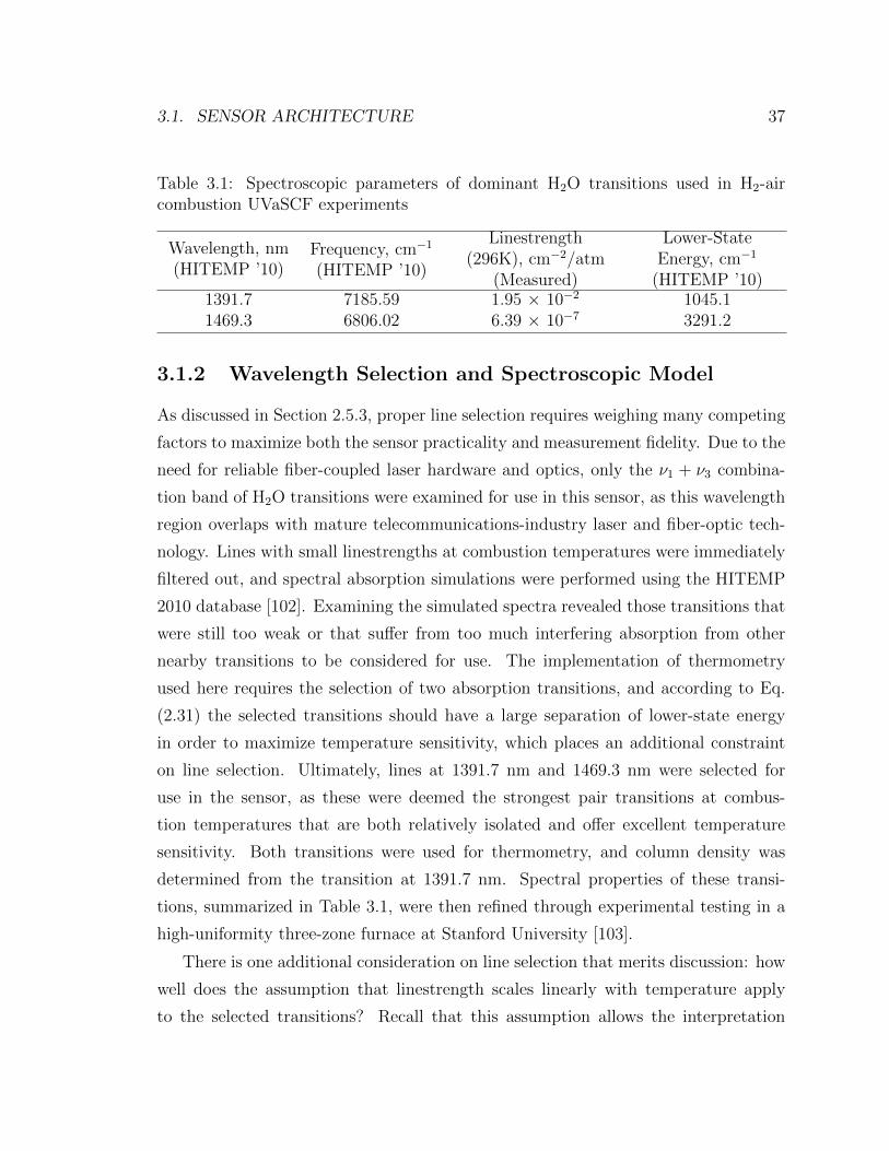
3.1. SENSOR ARCHITECTURE 37
Table 3.1: Spectroscopic parameters of dominant H2O transitions used in H2-aircombustion UVaSCF experiments
Wavelength, nm(HITEMP ’10)
Frequency, cm−1
(HITEMP ’10)
Linestrength(296K), cm−2/atm
(Measured)
Lower-StateEnergy, cm−1
(HITEMP ’10)1391.7 7185.59 1.95 × 10⁻² 1045.11469.3 6806.02 6.39 × 10⁻⁷ 3291.2
3.1.2 Wavelength Selection and Spectroscopic Model
As discussed in Section 2.5.3, proper line selection requires weighing many competing
factors to maximize both the sensor practicality and measurement fidelity. Due to the
need for reliable fiber-coupled laser hardware and optics, only the ν1 + ν3 combina-
tion band of H2O transitions were examined for use in this sensor, as this wavelength
region overlaps with mature telecommunications-industry laser and fiber-optic tech-
nology. Lines with small linestrengths at combustion temperatures were immediately
filtered out, and spectral absorption simulations were performed using the HITEMP
2010 database [102]. Examining the simulated spectra revealed those transitions that
were still too weak or that suffer from too much interfering absorption from other
nearby transitions to be considered for use. The implementation of thermometry
used here requires the selection of two absorption transitions, and according to Eq.
(2.31) the selected transitions should have a large separation of lower-state energy
in order to maximize temperature sensitivity, which places an additional constraint
on line selection. Ultimately, lines at 1391.7 nm and 1469.3 nm were selected for
use in the sensor, as these were deemed the strongest pair transitions at combus-
tion temperatures that are both relatively isolated and offer excellent temperature
sensitivity. Both transitions were used for thermometry, and column density was
determined from the transition at 1391.7 nm. Spectral properties of these transi-
tions, summarized in Table 3.1, were then refined through experimental testing in a
high-uniformity three-zone furnace at Stanford University [103].
There is one additional consideration on line selection that merits discussion: how
well does the assumption that linestrength scales linearly with temperature apply
to the selected transitions? Recall that this assumption allows the interpretation

38 CHAPTER 3. MEASUREMENTS IN AN H2-FUELED SCRAMJET
that measured signals from both direct-absorption and WMS measurements through
nonuniform flows will yield the species number-density-weighted path-average tem-
perature. However, in reality the linestrength is never perfectly linear across any
meaningful temperature range, and therefore it is helpful to quantify how linear the
behavior of S(T ) is over the expected nonuniformity across the path length. This
is plotted in Fig. 3.3, which shows the maximum percent error between the actual
linestrength function S(T ) and its linear approximation, aT + b, for a 500 K temper-
ature variation along the LOS and as a function of the mean temperature along the
LOS. Both of the selected transitions have errors of less than 4% for average temper-
atures above 1400 K, which is within the range of the vast majority of measurements
presented here. This implies that only small errors are introduced to the data analysis
when assuming that linestrengths scale linearly with temperature.
1400 1600 1800 2000 22000
1
2
3
4
5
Mean Temperature, K
Err
or
in L
inear
S(T
) A
ppro
x., (
% o
f S
(Tm
ean))
ν0 = 7185.59 cm
−1, E’’ = 1045.1 cm
−1
ν0 = 6806.02 cm
−1, E’’ = 3291.2 cm
−1
Results shown forT = T
mean ± 250 K
Figure 3.3: Error in a linear linestrength approximation as a function of mean tem-perature across the LOS for the spectroscopic transitions with E ′′ = 1045.1 cm−1 andE ′′ = 3291.2 cm−1 used in the UVaSCF Configuration A and C experiments.

3.1. SENSOR ARCHITECTURE 39
3.1.3 TDLAS Sensor Description
Figure 3.4 shows the layout of the TDLAS hardware used in the measurements.
Both lasers and data acquisition hardware were placed in a control room adjacent to
the tunnel room. Two separate lasers provided fiber-coupled light near 1391.7 nm
and 1469.3 nm, which were combined onto a single-mode polarization-maintaining
fiber optic and routed to the tunnel room. A ThorLabs F240APC-C lens was used
to collimate the output light into a free-space beam with an approximate diameter
of 1.5 mm, which was then directed across the combustor duct. The transmitted
light was collected through a 1 cm (maximum) aperture, followed by a 25 mm focal-
length mirror turning light 90 degrees (Configuration A measurements) or a 12 mm
f2 lens (Configuration C measurements). In both measurements, the focused light
was directed onto a 3 mm ScienceTech InGaAs photodetector (3 MHz bandwidth
subsequently anti-aliasing filtered to 1 MHz). For direct absorption measurements the
signal at the two wavelengths was demultiplexed in time. For WMS measurements
the two colors were demultiplexed by modulation frequency. The laser at 1391.7 nm
was modulated at 160 kHz and the laser at 1469.3 nm was modulated at 200 kHz,
with modulation depths selected to achieve approximately m = 2.2 over the range
of conditions in the combustor. In both measurement techniques the laser slow-scan
was at 250 Hz over a large enough amplitude to capture the entire lineshape.
As shown in Fig. 3.5, the entire optical assembly was attached to a set of computer-
controlled translation stages (Zaber, Inc.) that were controlled remotely, and allowed
the TDLAS LOS to span 15 cm of travel in the axial direction along the duct and 5
cm in the transverse direction across the duct. In Configuration A measurements, the
transverse translation stages sat on platforms and used a focusing mirror to turn light
90 degree into the detector, whereas for Configuration C measurements a linear setup
using a focusing lens was adopted. The primary advantage of the Configuration C
optical setup was to allow room for an additional beam path to enable Doppler-shift
velocity measurements (discussed in Section 2.4). Measurements focused on axial
locations of x/H = -10 (combustor inlet) and x = 0 for steam-added tests and x/H
= 6, x/H =12, x/H =15, and x/H =18 for various combustion tests, where H = 6.4
mm is the injector ramp height. In each axial measurement plane, measurement LOS

40 CHAPTER 3. MEASUREMENTS IN AN H2-FUELED SCRAMJET
Figure 3.4: Diagram of TDLAS system in relation to UVaSCF facility.
were spaced evenly by 1.5 mm, corresponding to the laser beam diameter, totaling
up to 24 separate LOS per plane (recall the duct expands at 2.9◦ downstream of fuel
injection). The optics were located several cm off of the outer face of the window, and
the ambient path was purged with N2 to limit absorption from H2O present in the
lab air. A small amount of remaining background absorbance was subtracted from
the measured signals.
Measurements reported here were obtained using an iterative combination of
direct-absorption and peak-WMS-2f /1f. This approach was taken because the peak-
WMS signal is sensitive to the lineshape just as the peak-direct-absorption signal is
(see Eq. (2.2)) and significant nonuniformity in temperature and composition were
expected along the LOS. Nonuniformity manifests itself as a nonuniform linewidth in
the measured spectra. Therefore, a separate in situ measurement of the empirical col-
lision linewidth was obtained from a Voigt lineshape fit to scanned-direct-absorption

3.1. SENSOR ARCHITECTURE 41
15 cm Translation Stages
5 cm Translation Stage
Transmission Optics
(fiber optics +
collimating lens)
Detector
Large Quartz
Viewing Windows
Nozzle
Flow Direction
Configuration A
=40°
Configuration C
Figure 3.5: Rendered images of TDLAS optical setup for Configuration A and Cexperiments, respectively.
measurements (see Fig. 3.6), as described in Section 2.5.3. The measured effective
linewidth was then fixed within WMS data processing of the WMS-2f /1f signal at
the location of the WMS-2f peak (see Fig. 3.7). See Appendix A for a detailed
exposition on how peak-WMS measurements with a fixed linewidth are converted
to quantitative temperature and column density measurements. Although methods

42 CHAPTER 3. MEASUREMENTS IN AN H2-FUELED SCRAMJET
have been proposed to recover the direct-absorption lineshape from WMS signals
directly (for example, see Ref. [104]), this iterative approach was chosen because
direct-absorption spectroscopy offers a simple interpretation that helps ensure that
the more complicated WMS signals are understood correctly.
7185.4 7185.5 7185.6 7185.7 7185.8−0.01
0
0.01
0.02
0.03
0.04
0.05
Absorb
ance
Relative Frequency (cm−1
)
Measured AbsorbanceAbsorbance Voigt Fit
Figure 3.6: Single-scan absorbance profile for absorption feature near 1391.7 nm,measured within the University of Virginia scramjet combustor (Configuration C)using scanned-direct-absorption at a location approximately 7.62 cm downstream offuel injection and 4.5 mm from the injector-side wall. Data was collected during H2-aircombustion experiments at equivalence ratio Φ = 0.17. A best-fit Voigt function, usedto measure the empirical collision linewidth, is shown overlaid on top of measuredabsorbance.
3.2 Uncertainty Analysis of WMS Measurements
Through Nonuniform Scramjet Flow
Two primary effects complicate the absorption of light propagating in a nonuniform
environment: 1) variation in gas temperature and absorbing species number den-
sity cause the integrated absorbance to vary in each volumetric element along the
LOS, and 2) variation in temperature, pressure and composition all cause the tran-
sition lineshape to change along the LOS. As a result, precise interpretation of the
measured path-integrated absorbance spectra requires knowledge of the distribution

3.2. UNCERTAINTY ANALYSIS OF WMS MEASUREMENTS 43
39.5 40 40.5 410.02
0.03
0.04
Time, msW
MS
−1f S
ignal
39.5 40 40.5 410
2
4x 10
−3
Time, ms
WM
S−
2f S
ignal
39.5 40 40.5 410
0.05
0.1
0.15
0.2
0.25
Time, ms
WM
S−
2f/1f S
ignal
a)
b)c)
Figure 3.7: WMS 2f, 1f, and 2f /1f signals for the H2O transition near 1391.7 nmmeasured in the University of Virginia supersonic combustor (Configuration C) ata location approximately 7.62 cm downstream of fuel injection and 4.5 mm fromthe injector-side wall. Data was collected during H2-air combustion experiments atequivalence ratio Φ =0.17.
functions describing the variations in gas state across the LOS. While this can be done
using CFD results, which provide spatially-resolved temperature, pressure, and gas
composition, the extraction of flow field parameters (temperature, column density,
etc.) from measured TDLAS data relies on strategies that either model the nonuni-
formities along the LOS with path-averaged thermodynamic quantities, assume the
nonuniform conditions are distributed according to user-selected functions with input
parameters that are inferred using absorption signals over multiple transitions [105],
or use a more complicated hardware and data reduction system for tomographic
imaging of nonuniform conditions [106]. The former strategy was used in the analysis
of the TDLAS data measured here, and CFD simulations are used to estimate the
error introduced by using path-averaged thermodynamic quantities coupled with an
empirical lineshape function.
Because of the difference in the collisional-broadening efficiency of H2O and N2,
the transition linewidth varies by a factor of 5 between a gas composed of pure N2
and pure H2O. For the H2-air combustion presented here at a global equivalence
ratio of Φ = 0.17, the average water vapor mole fraction is 6.9% in equilibrium

44 CHAPTER 3. MEASUREMENTS IN AN H2-FUELED SCRAMJET
combustion products. However, the combustion products are not uniformly mixed,
and the maximum water vapor mole fraction predicted in any CFD volume element is
31.2%. To examine the effects of the nonuniform flow field on the quantities inferred
from the TDLAS data, the CFD solution was used to simulate the H2O absorption in
each volume element along each measurement LOS. Then, the total absorption was
calculated by integrating along the LOS (evaluating Eq. (2.2)) and a best-fit Voigt
profile was fit to the absorption lineshape to find the effective lineshape. Peak-WMS
signals from the CFD-simulated-absorption were then least-squares fit to simulations
fixing the linewidth to the effective value and using uniform conditions to determine
temperature and column density. This process directly replicates the data reduction
method used for the scramjet combustor measurements. These simulated-TDLAS
signals from the CFD solution implied that temperatures inferred from the ratio of
path-integrated peak-WMS signals were within 5.5% of the water-weighted average
CFD temperature at all locations and that the column density determined from a
peak-WMS signal agreed with its absolute CFD value within 3% at x/H = 6 and x/H
= 12, and within 6% at x/H = 18. Thus, even though the flow field has nonuniform
temperature and water distributions, the flow parameters determined from TDLAS
measurements in this nonuniform flow have only modest errors and are sufficiently
accurate to allow useful comparisons with CFD simulations of this complex flow field.
It is worth noting that this level of accuracy is only possible because of the effective
lineshape measurements used here, as discussed in Section 2.5.1.
3.3 TDLAS Measurements: “Configuration A”
3.3.1 Φ = 0.17 Equivalence Ratio Combustion Results
Combustion runs with dry air were conducted during steady facility operation us-
ing the scanned-wavelength WMS-2f sensor at Φ = 0.17 equivalence ratio on the
Configuration A combustor geometry. Both temperature and column density were
determined across the width of the combustor with a resolution of approximately 1.5
mm at each of two measurement planes downstream of fuel injection (at distances

3.3. TDLAS MEASUREMENTS: “CONFIGURATION A” 45
x/H = 12 and x/H = 18, normalized by fuel-injector ramp height H = 6.4 mm).
Because the flow path diverged linearly along the fuel-injector wall, the measurement
plane at x/H = 18 was approximately 2 mm wider than x/H = 12. The width of
the duct (y-direction) was 2.58 cm at the injector and 3.34 cm at x/H = 18. At each
measurement point, 0.5 seconds of WMS-2f data was collected at a bandwidth of 250
Hz (WMS scan frequency) and with modulation frequencies of 160 kHz and 200 kHz
for lines at 1391.7 nm and 1469.3 nm respectively. Reported values are the average
over this sample time, with example uncertainty bars reported based on statistical
precision of one standard deviation in WMS signal measurements (Note these error
assessments are repeated in Fig. 3.8-3.10). Results are shown with the abscissa de-
noted as distance from the wall opposite the fuel-injector. This was done because the
fuel injector was along the angled wall and therefore the fuel injector wall is along the
right edge of each graph. For ease of comparison with other diagnostic measurements
(e.g. Refs. [97, 100]), the top of each graph shows the abscissa with non-dimensional
units of distance normalized by ramp-height, y/H.
Results for TDLAS column density and temperature measurements are shown in
Fig. 3.8 for measurement planes x/H = 12 and x/H = 18. Column density results
in Fig. 3.8a reveal a plume of products downstream of the fuel injector penetrating
successively greater distances into the flow to a maximum of about 2.5 cm at x/H
= 18. Throughout much of the product plume there is a significant increase in peak
column density between x/H = 12 and x/H = 18 corresponding to increased com-
bustion progress with axial distance. For both planes, peak column densities occur
near the center of the product plume before descending rapidly towards zero at the
plume edge farthest from the fuel injector ramp. Along the wall downstream of the
fuel injector ramp, only a small rise in H2O products is observed between x/H = 12
and x/H = 18. Note the measurement value for x/H = 12 closest to the injector
wall appears unusually large. Possibly this point was perturbed by interference of
transmission from reflections by the wall in the vibrating combustor. These qualita-
tive assessments of the TDLAS measurements are in good agreement with PLIF and
CARS data [33, 97].

46 CHAPTER 3. MEASUREMENTS IN AN H2-FUELED SCRAMJET
−2 −1 0 1 2 3
0
0.2
0.4
0.6
0 1 2 30
0.2
0.4
0.6
y/H
Distance from Wall Opposite Injector, cm
H2O
Co
lum
n D
en
sity,
g m
−2
x/H = 18 TDLASx/H = 12 TDLAS
a)
−2 −1 0 1 2 3
800
1200
1600
2000
2400
0 1 2 3800
1200
1600
2000
2400
y/H
Distance from Wall Opposite Injector, cm
H2O
−A
ve
rage
d T
em
pera
ture
, K
x/H = 18 TDLASx/H = 12 TDLAS
b)
Figure 3.8: TDLAS Measurement results for φ = 0.17 combustion in UVa CombustorConfiguration A. a) Water column density, b) Path-averaged temperature
Figure 3.8b shows the corresponding path-averaged H2O temperature measure-
ments for Φ = 0.17 combustion. Over most of the product plume successive planes
(i.e., at increasing axial distance from the injector) show significant increases in tem-
perature, up to a peak of nearly 1900 K at x/H = 18. Recall the TDLAS temperature
was determined from H2O absorption. Thus in regions where H2O column density
is small no temperature is reported. The free stream static temperature was 770 K,
thus the H2O absorption reveals elevated temperatures from combustion heat release
near the injector wall. At the edge of the combustion product plume farthest from
the fuel injector wall the temperature rolls off gradually, as expected.
3.3.2 Comparisons of TDLAS Data with CFD Simulations
Hybrid large eddy simulation/Reynolds-averaged Navier-Stokes CFD computations
were performed at North Carolina State University on the same scramjet combustor
geometry and reported in Ref. [86]. To compare these simulations with the TDLAS
measurements, column density was computed from the spatially-resolved simulation
by directly integrating H2O partial density results along the LOS corresponding to
the TDLAS measurement locations. The TDLAS determines temperature from water
vapor absorption; thus, a water-weighted temperature was computed from the CFD
using Eq. 2.5 to compare with the measured TDLAS temperature.
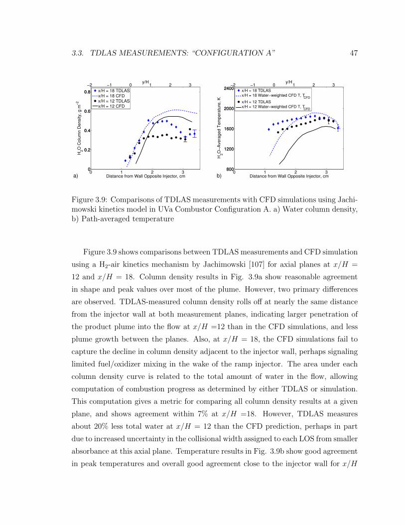
3.3. TDLAS MEASUREMENTS: “CONFIGURATION A” 47
−2 −1 0 1 2 3
0
0.2
0.4
0.6
0.8
0 1 2 30
0.2
0.4
0.6
0.8
y/H
Distance from Wall Opposite Injector, cm
H2O
Co
lum
n D
en
sity,
g m
−2
x/H = 18 TDLASx/H = 18 CFDx/H = 12 TDLASx/H = 12 CFD
a)
−2 −1 0 1 2 3
800
1200
1600
2000
2400
0 1 2 3800
1200
1600
2000
2400
y/H
Distance from Wall Opposite Injector, cm
H2O
−A
ve
rage
d T
em
pera
ture
, K
x/H = 18 TDLASx/H = 18 Water−weighted CFD T, T
CFD
x/H = 12 TDLASx/H = 12 Water−weighted CFD T, T
CFD
b)
Figure 3.9: Comparisons of TDLAS measurements with CFD simulations using Jachi-mowski kinetics model in UVa Combustor Configuration A. a) Water column density,b) Path-averaged temperature
Figure 3.9 shows comparisons between TDLAS measurements and CFD simulation
using a H2-air kinetics mechanism by Jachimowski [107] for axial planes at x/H =
12 and x/H = 18. Column density results in Fig. 3.9a show reasonable agreement
in shape and peak values over most of the plume. However, two primary differences
are observed. TDLAS-measured column density rolls off at nearly the same distance
from the injector wall at both measurement planes, indicating larger penetration of
the product plume into the flow at x/H =12 than in the CFD simulations, and less
plume growth between the planes. Also, at x/H = 18, the CFD simulations fail to
capture the decline in column density adjacent to the injector wall, perhaps signaling
limited fuel/oxidizer mixing in the wake of the ramp injector. The area under each
column density curve is related to the total amount of water in the flow, allowing
computation of combustion progress as determined by either TDLAS or simulation.
This computation gives a metric for comparing all column density results at a given
plane, and shows agreement within 7% at x/H =18. However, TDLAS measures
about 20% less total water at x/H = 12 than the CFD prediction, perhaps in part
due to increased uncertainty in the collisional width assigned to each LOS from smaller
absorbance at this axial plane. Temperature results in Fig. 3.9b show good agreement
in peak temperatures and overall good agreement close to the injector wall for x/H

48 CHAPTER 3. MEASUREMENTS IN AN H2-FUELED SCRAMJET
= 18, but for x/H = 12, the TDLAS value of water-weighted average temperature
is about 200 K higher at some points in the plume core. Coupled with the reduced
amount of H2O seen in the column density results at x/H = 12, this suggests there
was less heat transfer from the combustion products to unreacted gas than CFD
predicts.This idea is supported by the fact that TDLAS measurements show the
water remained much hotter than the CFD water-weighted mixture temperature far
from the injector wall as temperature rolls off at the plume edge.
−2 −1 0 1 2 3
0
0.2
0.4
0.6
0.8
0 1 2 30
0.2
0.4
0.6
0.8
y/H
Distance from Wall Opposite Injector, cm
H2O
Colu
mn D
ensity,
g m
−2
x/H = 18 TDLASx/H = 18 CFDx/H = 12 TDLASx/H = 12 CFD
a)
−2 −1 0 1 2 3
800
1200
1600
2000
2400
0 1 2 3800
1200
1600
2000
2400
y/H
Distance from Wall Opposite Injector, cm
H2O
−A
vera
ged
Tem
pera
ture
, K
x/H = 18 TDLASx/H = 18 Water−weighted CFD T, T
CFD
x/H = 12 TDLASx/H = 12 Water−weighted CFD T, T
CFD
b)
Figure 3.10: Comparisons of TDLAS measurements with CFD simulations usingBurke kinetics model in UVa Combustor Configuration A. a) Water column density,b) Path-averaged temperature
CFD simulations were also performed using a H2-air chemical mechanism by
Burke, et al. [108]. The same comparison methods used for the Jachimowski-kinetics
CFD were used for this simulation, and the resulting column density and tempera-
ture comparisons are shown in Fig. 3.10. The profile shapes for both column density
and temperature are largely unchanged and therefore many of the same conclusions
can be drawn in comparing TDLAS data to CFD prediction of plume shape. One
important distinction is that column density results in Fig. 3.10a show that the CFD
with Burke, et al. kinetics predicts higher peak values of the H2O column density
compared to measurements, particularly near the injector wall. The Burke-kinetics
CFD also predicts that the product plume penetrates slightly farther into the flow
at both planes. This produces better plume penetration agreement at x/H = 12,

3.4. TDLAS MEASUREMENTS: “CONFIGURATION C” 49
but at x/H = 18, the Burke-based CFD does not agree with measurement as well as
the Jachimowski mechanism. Taken together with the increased peak column densi-
ties, the conclusion is that the Burke chemical mechanism predicts more combustion
progress than the Jachimowski mechanism. Such increased combustion progress im-
plies greater heat release, which can be seen in a comparison of temperature results
in Fig. 3.10b. In this case, the CFD predicts slightly higher peak temperatures com-
pared to the Jachimowski results. Although this difference is small, it does in fact
reduce the disparity between TDLAS and CFD at x/H = 12.
3.4 TDLAS Measurements: “Configuration C”
As in results reported for the Configuration A combustor geometry, the following
figures show measurements with the abscissa representing distance across the trans-
verse direction (y-direction) along successive axial x-planes. Distances between the
TDLAS LOS on the abscissa have an origin at the wall opposite the injector because
the injector-side wall diverges at 2.9 degrees beginning at the base of the fuel injector
ramp. At each measurement point 0.5 seconds of data were collected resulting in 250
scans for the WMS technique and 125 scans for direct absorption. The facility oper-
ation was found to be quite steady, and hence only the average values are reported
here. Quoted uncertainty levels were calculated from the propagation of random er-
rors based on one standard deviation in measured signals. Error bars are shown for
only a single point but are representative of the entire plane.
3.4.1 Steam Addition Measurements
Steam was added to the flow for non-combustion tests to validate the facility hardware
and sensor performance for a uniform flow with known pressure, temperature, and
H2O concentration. Here, temperature and column density was measured upstream
of the fuel injector at x/H = -10. These data provide validated boundary conditions
for CFD models; in particular any irregularities found in experimental measurements
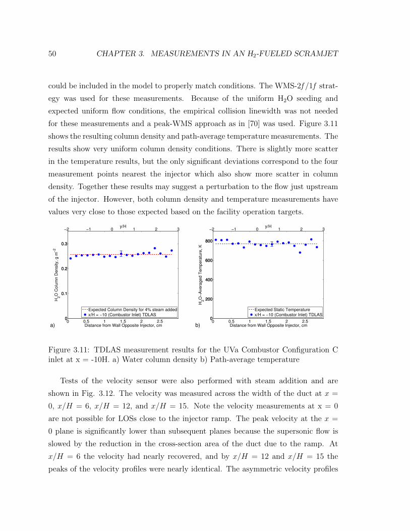
50 CHAPTER 3. MEASUREMENTS IN AN H2-FUELED SCRAMJET
could be included in the model to properly match conditions. The WMS-2f /1f strat-
egy was used for these measurements. Because of the uniform H2O seeding and
expected uniform flow conditions, the empirical collision linewidth was not needed
for these measurements and a peak-WMS approach as in [70] was used. Figure 3.11
shows the resulting column density and path-average temperature measurements. The
results show very uniform column density conditions. There is slightly more scatter
in the temperature results, but the only significant deviations correspond to the four
measurement points nearest the injector which also show more scatter in column
density. Together these results may suggest a perturbation to the flow just upstream
of the injector. However, both column density and temperature measurements have
values very close to those expected based on the facility operation targets.
−2 −1 0 1 2 3
0
0.1
0.2
0.3
0 0.5 1 1.5 2 2.50
0.1
0.2
0.3
y/H
Distance from Wall Opposite Injector, cm
H2O
Co
lum
n D
en
sity,
g m
−2
Expected Column Density for 4% steam addedx/H = −10 (Combustor Inlet) TDLAS
a)
−2 −1 0 1 2 3
0
200
400
600
800
0 0.5 1 1.5 2 2.50
200
400
600
800
y/H
Distance from Wall Opposite Injector, cm
H2O
−A
ve
rag
ed
Te
mp
era
ture
, K
Expected Static Temperaturex/H = −10 (Combustor Inlet) TDLAS
b)
Figure 3.11: TDLAS measurement results for the UVa Combustor Configuration Cinlet at x = -10H. a) Water column density b) Path-average temperature
Tests of the velocity sensor were also performed with steam addition and are
shown in Fig. 3.12. The velocity was measured across the width of the duct at x =
0, x/H = 6, x/H = 12, and x/H = 15. Note the velocity measurements at x = 0
are not possible for LOSs close to the injector ramp. The peak velocity at the x =
0 plane is significantly lower than subsequent planes because the supersonic flow is
slowed by the reduction in the cross-section area of the duct due to the ramp. At
x/H = 6 the velocity had nearly recovered, and by x/H = 12 and x/H = 15 the
peaks of the velocity profiles were nearly identical. The asymmetric velocity profiles
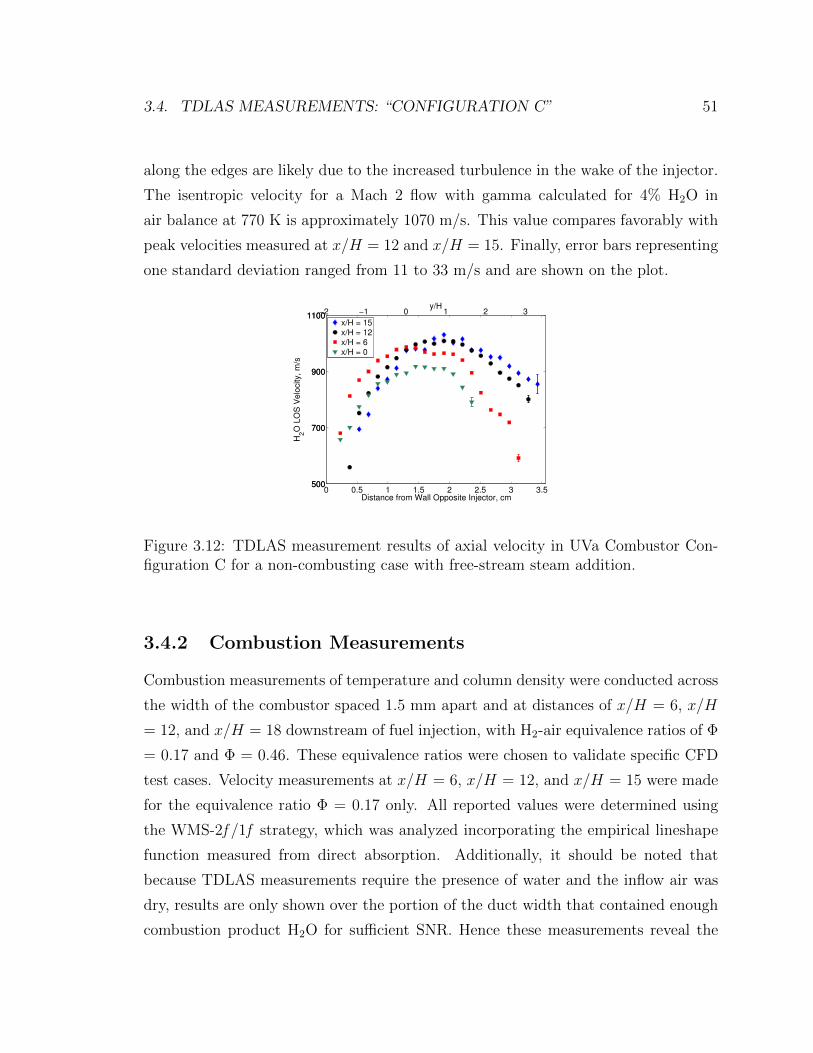
3.4. TDLAS MEASUREMENTS: “CONFIGURATION C” 51
along the edges are likely due to the increased turbulence in the wake of the injector.
The isentropic velocity for a Mach 2 flow with gamma calculated for 4% H2O in
air balance at 770 K is approximately 1070 m/s. This value compares favorably with
peak velocities measured at x/H = 12 and x/H = 15. Finally, error bars representing
one standard deviation ranged from 11 to 33 m/s and are shown on the plot.
−2 −1 0 1 2 3
500
700
900
1100
0 0.5 1 1.5 2 2.5 3 3.5500
700
900
1100y/H
Distance from Wall Opposite Injector, cm
H2O
LO
S V
elo
city, m
/s
x/H = 15x/H = 12x/H = 6x/H = 0
Figure 3.12: TDLAS measurement results of axial velocity in UVa Combustor Con-figuration C for a non-combusting case with free-stream steam addition.
3.4.2 Combustion Measurements
Combustion measurements of temperature and column density were conducted across
the width of the combustor spaced 1.5 mm apart and at distances of x/H = 6, x/H
= 12, and x/H = 18 downstream of fuel injection, with H2-air equivalence ratios of Φ
= 0.17 and Φ = 0.46. These equivalence ratios were chosen to validate specific CFD
test cases. Velocity measurements at x/H = 6, x/H = 12, and x/H = 15 were made
for the equivalence ratio Φ = 0.17 only. All reported values were determined using
the WMS-2f /1f strategy, which was analyzed incorporating the empirical lineshape
function measured from direct absorption. Additionally, it should be noted that
because TDLAS measurements require the presence of water and the inflow air was
dry, results are only shown over the portion of the duct width that contained enough
combustion product H2O for sufficient SNR. Hence these measurements reveal the

52 CHAPTER 3. MEASUREMENTS IN AN H2-FUELED SCRAMJET
development of the combustion product plume with increasing axial distance from
the fuel injector.
Φ = 0.17 Equivalence Ratio Combustion Results
TDLAS measurements of column density shown in Fig. 3.13a reveal the combustion
product plume grows significantly with each successive axial plane. Many simple
metrics show this behavior: the peak value of column density increases at each plane,
the transverse penetration of H2O increases, and finally the total area under the
column density curve - which is directly related to overall combustion progress -
increases significantly between each plane. The most significant rise in column density
is seen between x/H = 12 and x/H = 18, where the core of the product plume rises
from about 0.4 g/m2 to 0.7 g/m2. Close to the injector wall, there is very little rise
in column density at any location. This may indicate limited combustion progress
near the injector wall between the TDLAS measurement planes. Fig. 3.13b shows
corresponding TDLAS temperatures (H2O-weighted) for this combustion case. The
temperature results reinforce conclusions drawn from the column density results. Near
the injector wall, the temperature is more than 1400 K by x/H =6, but rises about
200 K between x/H = 6 and x/H = 18. Because heat transfer to the wall would
likely be a dominant effect only near boundary layers and not well into the combustion
product plume as observed in the results, this effect likely indicates little heat release
from combustion between x/H = 6 and x/H = 18. Farther from the injector wall
the temperature rise between each plane is significant, indicating more combustion
progress.
CFD calculations using a hybrid large-eddy simulation/Reynolds-averaged Navier-
Stokes approach on the Configuration C combustor geometry and conditions were
performed at North Caroline State University using a chemistry mechanism from
Burke, et al. [108]. CFD-calculated column density computed via Eq. (2.6) are
also shown in Fig. 3.13a as dashed and solid lines. Across all three planes, there
is modest agreement in the magnitude of column density. Agreement is best just
downstream of the injector at x/H = 6, but by x/H = 18 TDLAS measurements
show both a higher peak column density magnitude and a different peak location.

3.4. TDLAS MEASUREMENTS: “CONFIGURATION C” 53
TDLAS measurements also show that H2O products penetrate farther into the flow
than the CFD predicts. In the immediate wake of the injector ramp, CFD captures
some of the limited combustion progress observed by TDLAS, however it still tends
to over-predict H2O in this region. CFD-computed temperatures were determined
from the H2O-weighted average temperature over the LOS and are shown in Fig.
3.13b. There is good agreement between CFD and TDLAS measurements across
all three measurement planes close to the injector wall, however farther from the
injector wall TDLAS measurements show higher temperatures than CFD predicts.
This makes some sense because the TDLAS measurements show the product plume
extends farther into the flow, and we expect higher temperatures wherever there are
hot combustion products. Another possible explanation is that the CFD over-predicts
heat transfer from the combustion products to the free stream gas gas since the sensor
measured the static temperature of H2O. This plume-edge behavior is consistent with
the Configuration A measurements presented in section 3.3.1.
−2 −1 0 1 2 3
0
0.2
0.4
0.6
0.8
0 0.5 1 1.5 2 2.5 3 3.50
0.2
0.4
0.6
0.8
y/H
Distance from Wall Opposite Injector, cm
H2O
Co
lum
n D
en
sity,
g m
−2
x/H = 18 TDLASx/H = 18 CFDx/H = 12 TDLASx/H = 12 CFDx/H = 6 TDLASx/H = 6 CFD
a)
−2 −1 0 1 2 3
500
700
900
1100
1300
1500
1700
1900
2100
0 0.5 1 1.5 2 2.5 3 3.5500
700
900
1100
1300
1500
1700
1900
2100
y/H
Distance from Wall Opposite Injector, cm
H2O
−A
ve
rag
ed
Te
mp
era
ture
, K
x/H = 18 TDLASx/H = 18 H
2O−avg. CFD T
x/H = 12 TDLASx/H = 12 H
2O−avg. CFD T
x/H = 6 TDLASx/H = 6 H
2O−avg. CFD T
b)
Figure 3.13: TDLAS measurement results compared to CFD simulation for H2-aircombustion at equivalence ratio of Φ = 0.17, facility Configuration C. a) Water columndensity b) Path-average temperature
Measurements of axial velocity at x/H = 6, x/H = 12, and x/H = 15 for Φ = 0.17
global equivalence ratio combustion are shown in Fig. 3.14. Note that as with the
other combustion measurements, velocities are only shown over the product plume
where significant H2O concentrations provided sufficient signal for measurements.

54 CHAPTER 3. MEASUREMENTS IN AN H2-FUELED SCRAMJET
Near the injector wall the core flow velocity is significantly reduced compared to
the unmixed case (core velocity approximately 1070 m/s) shown in Fig. 3.12 due
to the addition and mixing of the fuel. Limited velocity recovery with downstream
progression was observed. Likewise, the edge of the plume far from the injector wall
showed significant velocity recovery towards the free stream values observed in the
unmixed case. CFD axial velocities are shown as the dashed and solid connected lines
in Fig. 3.14. The shape and magnitude of the velocity distribution shows excellent
agreement with CFD across the width of the duct, particularly at x/H = 6 and x/H
= 15. The plane at x/H = 12, however, shows some moderate discrepancy with
the TDLAS results suggesting CFD over-predicts velocity, however this difference is
contained by the experiment error bars. Far from the injector wall, near the edge of
the combustion product plume, the TDLAS measurement is much lower than CFD.
Measurements in this region of the flow suffer from increased uncertainty due to
small H2O concentrations at the combustion plume edge, which may explain this
discrepancy.
−2 −1 0 1 2 3
0
200
400
600
0 0.5 1 1.5 2 2.5 3 3.50
200
400
600
y/H
Distance from Wall Opposite Injector, cm
H2O
LO
S V
elo
city,
m/s
x/H = 15x/H = 15 H
2O−avg. CFD V
x/H = 12x/H = 12 H
2O−avg. CFD V
x/H = 6x/H = 6 H
2O−avg. CFD V
Figure 3.14: TDLAS measurement of axial velocity compared to CFD simulation forequivalence ratio of Φ = 0.17, facility Configuration C.
CARS measurements of H2, N2, and O2 mole fraction were made by Cutler, et al.
in the UVaSCF in the Configuration C geometry for the same H2-air equivalence ratio
Φ = 0.17 case at axial distances of x/H = 6 and x/H = 18 [33]. However, because

3.4. TDLAS MEASUREMENTS: “CONFIGURATION C” 55
CARS does not measure H2O directly, CARS-inferred H2O column density was calcu-
lated from χCARSH2O
= 1−χCARSH2
−χCARSN2
−χCARSO2
using the CARS measurements. This
equation is analogous to assuming complete combustion of consumed H2 and ignores
free atoms and radicals which are combustion intermediates. Therefore, the value
of χCARSH2O
is an upper bound on the amount of water. To compare with the TDLAS
data, χCARSH2O
was converted to column density by integration along the LOS. Note the
CFD predicts a mole fraction of combustion intermediates ranging from 0-8% along
the TDLAS measurement LOS. Because CARS measurements capture H2, N2, O2
concentrations and TDLAS measures H2O, the difference between the CARS-inferred
and TDLAS H2O column densities gives a measure of the local concentration of in-
termediate species in the product plume. Comparisons between the CARS-inferred
and TDLAS H2O column density are shown in Fig. 3.15a (x/H = 6) and 3.15b
(x/H = 18). These comparisons allow identification of two distinct regions of the
combustion product plume. For both planes, near the injector wall TDLAS column
density is significantly smaller than CARS-inferred column density, indicating that
this region of the flow contained large intermediate species concentrations and ongo-
ing chemistry in good agreement with CFD predictions. Near the edge of the product
plume, however, TDLAS measurements approach the CARS-inferred column density
values. This result suggests the complete combustion assumption of consumed H2
used for the CARS-inferred values is accurate at the plume edge and may perhaps
be interpreted that the combustion product H2O at these locations is the result of
transport as opposed to local reaction. Note that although CARS measurements also
report temperature, we do not include any comparisons with TDLAS measurements
because the H2O-weighted temperature using χCARSH2O
would contain significant errors
over large regions of the product plume where combustion is not complete and the
CARS-inferred H2O is inaccurate. Thus, meaningful comparisons between the two
temperature measurements are difficult to identify.
Φ = 0.46 Equivalence Ratio Combustion Results
Combustion tests at a fuel-air equivalence ratio of Φ = 0.46 were also performed and
TDLAS measurements of temperature and column density were obtained. Column

56 CHAPTER 3. MEASUREMENTS IN AN H2-FUELED SCRAMJET
−2 −1 0 1 2 3
0
0.2
0.4
0.6
0.8
0 0.5 1 1.5 2 2.5 3 3.50
0.2
0.4
0.6
0.8
y/H
Distance from Wall Opposite Injector, cm
H2O
Colu
mn D
ensity, g m
−2
CARS−inferredTDLASCFD
a)
−2 −1 0 1 2 3
0
0.2
0.4
0.6
0.8
0 0.5 1 1.5 2 2.5 3 3.50
0.2
0.4
0.6
0.8
y/H
Distance from Wall Opposite Injector, cm
H2O
Co
lum
n D
en
sity,
g m
−2
CARS−inferredTDLASCFD
b)
Figure 3.15: TDLAS measurements of H2O column density compared to CARS-inferred column density for H2-air combustion at equivalence ratio of Φ = 0.17, facilityConfiguration C. H2O column density is inferred from CARS by assuming completecombustion of consumed H2 fuel. a) Axial position x = 6H b) Axial position x = 18H
density results are shown in Fig. 3.16a and, as noted with Φ = 0.17 equivalence
ratio results, each successive measurement plane shows increasing column density
corresponding to combustion progress. Peak column densities are observed in the
center of the plume, although the rise in peak column density between successive
planes is limited. CFD predictions for this equivalence ratio are also shown in Fig.
3.16. There is reasonable agreement between TDLAS measurements and CFD at
the edges of the plume, indicating the CFD captures the plume penetration physics
well. However, peak values at the center of the combustion plume for the CFD
predictions are significantly larger than the TDLAS measurements. Temperatures
measured by TDLAS and corresponding H2O-averaged CFD temperatures are shown
in Fig. 3.16b. TH2O measurements show a large dip in temperature in the central
region of the product plume, possibility indicating limited combustion extent due to
the increased concentration of fuel in this richer stoichiometry, cooling of the flow
by the fuel injection, and the large momentum of the fuel jet. As with the lower
equivalence ratio case, the CFD temperature predictions show fairly good agreement
with TDLAS results. It does appear that the CFD solution tends to over-predict
the temperature slightly, which reinforces the conclusion from column density that
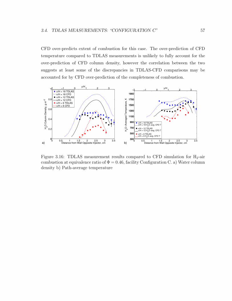
3.4. TDLAS MEASUREMENTS: “CONFIGURATION C” 57
CFD over-predicts extent of combustion for this case. The over-prediction of CFD
temperature compared to TDLAS measurements is unlikely to fully account for the
over-prediction of CFD column density, however the correlation between the two
suggests at least some of the discrepancies in TDLAS-CFD comparisons may be
accounted for by CFD over-prediction of the completeness of combustion.
−2 −1 0 1 2 3
00 0.5 1 1.5 2 2.5 3 3.5
0
0.2
0.4
0.6
0.8
1y/H
Distance from Wall Opposite Injector, cm
H2O
Colu
mn D
ensity, g m
−2
x/H = 18 TDLASx/H = 18 CFDx/H = 12 TDLASx/H = 12 CFDx/H = 6 TDLASx/H = 6 CFD
a)
−2 −1 0 1 2 3
300
500
700
900
1100
1300
1500
1700
1900
0 0.5 1 1.5 2 2.5 3 3.5300
500
700
900
1100
1300
1500
1700
1900
y/H
Distance from Wall Opposite Injector, cm
H2O
−A
vera
ged T
em
pera
ture
, K
x/H = 18 TDLASx/H = 18 H
2O−avg. CFD T
x/H = 12 TDLASx/H = 12 H
2O−avg. CFD T
x/H = 6 TDLASx/H = 6 H
2O−avg. CFD T
b)
Figure 3.16: TDLAS measurement results compared to CFD simulation for H2-aircombustion at equivalence ratio of Φ = 0.46, facility Configuration C. a) Water columndensity b) Path-average temperature

Chapter 4
Multispecies Measurements in a
Hydrocarbon-Fueled Scramjet
Combustor
While hydrogen fueled scramjets are primarily viewed as a potential source of low-
cost orbital vehicle propulsion, there is also substantial interest in hydrocarbon-fueled
scramjets, mostly for low-cost expendable vehicles to be used in defense applications
[10]. For these vehicles, hypersonic flight speeds greater than Mach 5 are of particular
interest [16, 109]. However, with hydrocarbon fuels, effects of the finite-rate chemistry
amplify already complicated considerations in scramjet combustor operation: hydro-
carbon fuels typically have ignition delay times that compete with fuel residence
times in the combustor and the greatly increased number of species make both mea-
surement strategies and computational models more complex. To that end, robust
diagnostic methods are needed to track combustion progress and aid understanding of
the gas dynamic behavior within hydrocarbon-fueled scramjet combustors. One use-
ful method is absorption spectroscopy, which has a long history of providing reliable
diagnostics that can withstand harsh scramjet conditions [26, 36, 61, 63, 93, 94, 110].
This chapter presents the results of multispecies spectroscopic diagnostic measure-
ments to detect the H2O and CO temperatures and H2O, CO, and CO2 column den-
sities in an ethylene-fueled direct-connect model scramjet combustor [25, 111, 112].
58
59
Tracking carbon species is vitally important within the scramjet combustor, and
strong CO and CO2 transitions with minimal interference from H2O are only avail-
able in the fundamental vibrational bands at wavelengths longer than 4 µm. For H2O
measurements near 2.5 µm, mid-infrared laser sources enable access to strong funda-
mental band absorption transitions that offer considerably larger signal-to-noise ratio
over sensors using telecommunications diode lasers probing overtone or combination
band (2ν1 and ν1 + ν3) transitions near 1.4 µm. Many earlier diode laser absorption
applications in scramjets have been restricted to measuring H2O using these robust
telecommunications devices [58, 59, 61]. Here we exploit new commercially-available
technology to access stronger fundamental band transitions to monitor CO and CO2
in addition to H2O. Fiber-coupling of the laser source to the aeroengine test article
provides needed robust hardware mounting and only recently have fiber solutions
become available for these mid-IR wavelengths for CO and CO2 [111, 113]. Measure-
ments presented in Chapter 3 from a similar hydrogen-fueled scramjet combustor ge-
ometry revealed the presence of nonuniformities in temperature and composition and
have shown they can introduce significant error in absorption measurements [95, 96].
However, use of mid-infrared absorption transitions allowed optimal line-selection to
account for nonuniform conditions [65]. Here, measurements of CO and H2O employed
the recently-described scanned-wavelength-modulation (scanned-WMS) spectroscopy
technique, which helps to account for nonuniform conditions along the LOS with in
situ measurements of the absorption lineshape obtained directly from the WMS line-
shape [84, 82]. Measurements of CO2 used an external cavity quantum cascade laser
source that was not capable of the rapid wavelength tuning needed for WMS mea-
surements, and thus CO2 column density was measured using scanned-wavelength
direct-absorption, which also provides an integrated in situ lineshape. Species were
measured sequentially; first simultaneous CO and CO2 data were acquired and then
runs were repeated three days later to acquire H2O data at the same facility condi-
tions. As in the H2-air scramjet combustor measurements presented in Chapter 3, the
measurement line-of-sight (LOS) was translated throughout the combustor to map
combustion progress across several planes downstream of fuel injection.
Results reveal peak temperatures of about 2200 K occur within the combustor

60 CHAPTER 4. MULTISPECIES MEASUREMENTS IN A SCRAMJET
flame-holding cavity. Downstream of the cavity no temperature rise occurs in ei-
ther CO or H2O, indicating competition between thermal dilution and combustion
progress. Column density measurements show increasing concentration of combustion
products downstream of the fuel injection, revealing the spatial evolution of combus-
tion progress. However, large concentrations of the intermediate CO species were
also observed, indicating incomplete combustion heat release. Error analysis indi-
cates only a small measurement uncertainty compared to the observed time-variation
of the data, and therefore these temporal fluctuations in combustion products likely
represent unsteady combustion. In addition, measurements of H2O were made in the
cavity during flame extinction that provide an upper bound on the cavity residence
time of about 3.4 ms. These measurements are the first demonstration of this tech-
nique, and the results offer a promising avenue to future direct measurements of the
cavity residence time in a supersonic flame holder, which is an important parameter
to aid understanding of competition between ignition delay and mass transport in
supersonic flows.
4.1 Mid-IR Absorption Transition Selection
Measurements in the UVaSCF presented several important challenges that were ad-
dressed in selecting the laser absorption transitions. Hydrocarbon fuel reduced the
expected H2O concentration compared to the previously-studied hydrogen-fueled case,
resulting in less absorption. Because there are multiple major product species in an
ethylene-air flame, multispecies measurements are a necessity if one hopes to generate
a complete view of combustion progress and efficiency. In addition, compared to the
chemistry that converts OH to H2O, the chemistry that converts CO to CO2 is no-
toriously slow, and measurements of both CO and CO2 are important to understand
incomplete combustion. Moreover, nonuniform conditions within the scramjet com-
bustor present a distinct challenge to any sensor design. Thus, here the species CO,
CO2, and H2O were selected for measurement, and Fig. 4.1 shows the linestrengths of
these species from 1-6 µm at 1500 K. Two transitions near 4.85 µm were selected for
CO measurements of temperature and column density, two transitions near 2.5 µm

4.1. MID-IR ABSORPTION TRANSITION SELECTION 61
Table 4.1: Spectroscopic parameters of H2O, CO, and CO2 transitions used inethylene-air combustion UVaSCF experiments.
SpeciesFrequency, cm−1
(HITEMP ’10)
Linestrength(296K), cm−2/atm
(Measured)
Lower-StateEnergy, cm−1
(HITEMP ’10)H2O 3920.09 63.5 × 10⁻² 704.214H2O 4030.73 26.8 × 10⁻¹⁰ 4889.488CO 2059.91 87.6 × 10⁻² 806.4CO 2060.33 26.4 × 10⁻⁵ 2543.1CO2 2394.42 73.9 × 10⁻⁶ 3329.0
for H2O measurements of temperature and column density, and a single transition
near 4.18 µm for CO2 measurements of column density (using the temperature pro-
vided by CO measurements and assuming the two species are in thermal equilibrium).
These transitions were selected based upon the sensor design studies by Goldenstein,
et al. [111] and Spearrin, et al. [113], and spectroscopic characteristics of the selected
transitions are summarized in Table 4.1.
4.85 m
4.18 m
2.48 m
Figure 4.1: CO, H2O, and CO2 spectra over a large range of infrared wavelengths at1500 K. The sensor presented targeted absorption transitions at wavelengths notedon the figure.
These mid-infrared transitions were selected not only to provide strong absorption

62 CHAPTER 4. MULTISPECIES MEASUREMENTS IN A SCRAMJET
signals and good temperature sensitivity, but also to minimize errors introduced by
assuming linestrength scales linearly with temperature, as discussed in Section 2.5.
Figure 4.2 shows the maximum percent deviation of the actual linestrength from a
linear approximation as a function of the mean temperature along the line of sight
for a temperature distribution spanning 500 K. These results are shown for all five
of the absorption transitions used in the results presented here, and confirm that
the errors introduced by this linear linestrength assumption are small, particularly
at high average temperatures such as those encountered in scramjet combustion.
Additionally, access to mid-infrared H2O absorption transitions allows for a more
than 50% reduced error in H2O linear linestrength approximation at temperatures
between 1300K and 1800 K compared to results presented in Section 3.1.2. This
translates directly to improved measurement fidelity in the results presented here.
1400 1600 1800 2000 22000
1
2
3
4
5
6
7
8
Mean Temperature, K
Err
or
in L
inear
S(T
) A
ppro
x., (
% o
f S
(Tm
ean))
H2O Transition, E’’ = 704.2 cm
−1
H2O Transition, E’’ = 4889.5 cm
−1
CO Transition, E’’ = 806.4 cm−1
CO Transition, E’’ = 2543.1 cm−1
CO2 Transition, E’’ = 3329.0 cm
−1
Results shown forT = T
mean ± 250 K
Figure 4.2: Error in a linear linestrength approximation for selected H2O, CO, andCO2 transitions as a function of mean temperature across the LOS.

4.2. FACILITY DESCRIPTION 63
4.2 Facility Description
Measurements were performed on the University of Virginia Supersonic Combustion
Facility (UVaSCF), in a slightly different combustor geometry configuration than the
measurements presented in Chapter 3. The UVaSCF is a direct-connect, continuous-
flow wind tunnel, as shown in Fig. 4.3. The facility was oriented vertically, with
the heater below ground, the test section above floor level, and with an atmospheric
exhaust through an open pipe to the roof of the building. Air was provided to the
facility by a compressor and desiccant dryer system [114]. Flow originated at the
top of a pressurized heater tank at 300 kPa and proceeded downward through an
outer annulus section before entering a 14-stage electrical-resistance heater core at
the bottom of the tank [115]. Air out of the heater had a total temperature of 1200 K,
making conditions equivalent to Mach 5 flight speeds. After leaving the heater, the
flow proceeded through a ceramic flow straightener and then a Mach 2 nozzle. The
nozzle was directly attached to a constant area isolator followed by the combustor.
Dimensions of the isolator section were 26.6 cm in length (x-axis), 2.54 cm in the
transverse direction (y-axis), and 3.81 cm along the LOS direction (z-axis). Within
the combustor and approximately 3.2 cm upstream of fuel injection, the flow path
diverged along the injector-side wall at an angle of 2.9 degrees. Heated ethylene was
injected through 5 ports spanning along the z-axis of the combustor 2.45 cm upstream
of the leading edge of a cavity flame holder [116]. The cavity had depth (y-direction)
of h = 0.9 cm and length 4.73 cm along the axial direction (x-axis) (L/D = 5.25), with
the rear edge of the cavity closed out with a ramp. There was optical access to the
combustor through large 20 cm by 6 cm fused-silica windows for H2O measurements
near 2.5 µm. Sidewalls with smaller slot-shaped sapphire windows at measurement
planes 1 and 2, noted in Fig. 4.3, allowed transmission of longer wavelengths (over 4
µm) for CO and CO2 measurements. All windows were wedged on the outer face to
avoid interference from internal etalon-type reflections as the laser wavelengths were
scanned. After the combustor, the flow continued through a 14.9 cm long constant
area section and an 18 cm long extender before exiting to the exhaust pipe.

64 CHAPTER 4. MULTISPECIES MEASUREMENTS IN A SCRAMJET
Y
X
Fuel Injection
Reaction Zone
Cavity
Plane 1
Plane 2
Plane 3
Free-Stream Recirculation
Zone
Flow Direction
Z
Combustor
Isolator Residence Time
Measurement
Figure 4.3: Photo of the UVaSCF direct-connect scramjet combustor (left) and car-toon diagram of the combustor and flame holder cavity configuration (right, not toscale) with three absorption spectroscopy measurement planes noted.
4.3 Absorption Spectroscopy Sensor Hardware
To simplify the hardware footprint and the combination of multiple wavelengths onto
one line-of-sight, simultaneous CO and CO2 measurements were first performed, then
H2O data was collected at the same facility conditions several days later. Figure
4.4 shows a diagram of the CO and CO2 measurement hardware. Two lasers were
used: a distributed-feedback quantum cascade laser (Alpes) near 4.87 µm for CO
measurements and an external cavity quantum cascade laser (Daylight Solutions)
near 4.2 µm for CO2 measurements. A mechanical beam chopper periodically blocked
the beam from the CO2 laser to measure the emission background signal needed
to correct the direct-absorption baseline. Light from each laser was independently
focused onto two hollow-core fibers (OKSI) via adjustable alignment stages, and the
two fibers combined into a common shield with the center of the two independent
fiber cores separated by 0.3 mm. Light out of the fiber pair was collimated by a 40
mm focal length silicon lens with the beam-centers separated by 1.5 mm and directed
through sapphire windows across UVaSCF combustor flow path. The beam was then
split onto two separate filtered mercury-cadmium-telluride (MCT) thermoelectrically
cooled detectors (Vigo) whose signals were digitized and saved.

4.3. ABSORPTION SPECTROSCOPY SENSOR HARDWARE 65
4.87 m
DFB QC Laser
(CO)
4.2 m
ECQC Laser
(CO2)
Multi-axis
Alignment
Stage
2-to-1 Fiber System
(Hollow-Core)
Beam Chopper (12.5 Hz)
CO/CO2 Sensor Hardware Layout
N2 purge of breadboard, hollow-core
fiber, and catch optics
100 Hz
Air
Flow
Combustor
Beam Splitter
Iris
Filter
MCT Detector
Lens40 mm f.l. Si Lens
200 Hz
50 kHz
+
Figure 4.4: CO and CO2 sensor hardware layout for hydrocarbon-fueled scramjettesting. The CO and CO2 lasers were both coupled through a single fiber and werede-multiplexed with a beam splitter after transmission through the combustor.
A sensor hardware diagram for H2O measurements is shown in Fig. 4.5. Light
originated in two distributed-feedback tunable diode lasers (nanoplus) emitting near
2551 nm and 2482 nm. Output light from each laser was collimated and passed onto
a beam splitter that combined both laser beams onto a single path. The multiplexed
light was focused onto a 400 µm-core multimode fiber (Fiberguide). At the combustor,
light was pitched across the test section by a 20 mm focal length zinc selenide lens.
Transmitted light was then filtered and focused onto a single MCT detector. The two
laser beams were demultiplexed in post-processing by isolating signals at modulation-
frequency harmonics harmonics (fm = 75 kHz for 2551 nm and 100 kHz for 2482 nm).
Lasers were scanned over absorption transitions with a 250 Hz sinusoid, resulting in
a repetition-rate of 500 Hz as each scan passed over the transition twice.
The position of the laser LOS in the combustor flow field for CO, CO2, and
H2O was mechanically translated using a set of computer-controlled high-precision
translation stages (Zaber). This stage system allowed the measurement LOS to span
up to 15 cm in the axial direction (x-axis) and 5 cm in the transverse direction (y-
axis). Measurements presented here focus on three axial planes 2.18 cm (Plane 1),
6.01 cm (Plane 2), and 9.83 cm (Plane 3) downstream of the cavity flame holder

66 CHAPTER 4. MULTISPECIES MEASUREMENTS IN A SCRAMJET
leading edge, as shown in Fig. 4.3.
2551 nm
DFB TDL laser
2482 nm
DFB TDL laser
H2O Sensor Hardware Layout
N2 purge of breadboard, fiber,
and catch optics
Air
Flow
Combustor
Filter
MCT Detector
Lens
20 mm f.l.
ZnSe Lens250 Hz
75 kHz
+
Beam Splitter
250 Hz
100 kHz
+
Collimating Lens
5-axis
Fiber-Mount
400 m
MM Fiber
Figure 4.5: H2O sensor hardware layout for hydrocarbon-fueled scramjet testing. Twodistributed feed-back tunable diode lasers were multiplexed onto a single fiber-opticline for simultaneous temperature and column density measurements.
4.4 Results
4.4.1 Multispecies Combustion Product Measurements
Combustion measurements were conducted at the UVaSCF for ethylene-air combus-
tion at a global equivalence ratio of Φ = 0.15. First, the CO and CO2 sensor was
used in a single run, then the H2O sensor was installed and measurements were made
in the following week at the same run conditions. As shown in Fig. 4.6, the axial
pressure trace from CO and CO2 testing overlaps strongly with the pressure trace
from H2O testing, indicating tunnel conditions are highly repeatable across different
runs and making comparisons between these sensor results from different times pos-
sible. Figure 4.6 also notes the three measurement planes, and shows all three planes
are downstream of the largest pressure rise due to the primary shocks. Measurement
results are shown for CO temperature and CO and CO2 column density in measure-
ment planes 1 and 2. Results for H2O temperature and column density are shown

4.4. RESULTS 67
for all three planes. In each plot, the abscissa is shown in units of distance from the
wall opposite the fuel injector. This convention was chosen because the wall opposite
the injector was straight; it did not diverge like the injector-side wall. The location
of the injector wall is noted on the plots for each plane. Each measurement point
represents the average over 1 s of integrated absorption data. H2O measurements
were acquired at a rate of 500 Hz, while CO and CO2 measurements were conducted
at 200 Hz and 100 Hz, respectively. Tunnel conditions are steady for time scales of
minutes or hours, with a 95% confidence interval of 1.5% in pressure [22], therefore
averaging absorption spectroscopy data tends to reduce random sensor noise. Error
bars shown are the standard deviation in measurements, but, as discussed below, they
are interpreted to represent the temporal fluctuations in combustion extent observed
over a particular LOS, rather than the measurement uncertainty.
−40 −30 −20 −10 0 10 20 30 40 50 600
0.1
0.2
0.3
0.4
0.5
0.6
0.7
0.8
0.9
1
Axial Distance (zero at cavity leading edge), cm
Pre
ssure
, atm
Fuel Off
φ=0.15, CO/CO2 Testing
φ=0.15, H2O Testing
Measurement Planes
Nozzle Exit
CombustorExit
Fuel Injection
Line Drawing of Axial Geometry
Figure 4.6: Axial pressure traces measured without fuel injection and with ethylenefuel injection at equivalence ratio of Φ = 0.15 for CO/CO2 testing and H2O testing.Also shown is a scale drawing of the axial geometry of the combustor.
CO and H2O temperature measurements are shown in Fig. 4.7, with subplot

68 CHAPTER 4. MULTISPECIES MEASUREMENTS IN A SCRAMJET
(a) showing data from Plane 2 and subplot (b) showing data from Plane 1. Note
that measurements from Plane 1 extend into the cavity flame holder. CO and H2O
temperature measurements agree within 17% at all locations, and with an average
difference of about 7%, suggesting that both species are distributed in regions of the
flame where temperatures are approximately equal. Peak temperatures from both
CO and H2O occur within the cavity where residence times are longest and there
is more time to oxidize complex molecules, resulting in temperatures in excess of
2150 K. Outside of the cavity in Fig. 4.7b, the temperature gradually descends to-
wards the free-stream static temperature of 770 K. However, note that measurements
only penetrate into the flow as far as there are substantial concentrations of com-
bustion products. Therefore, the measurements tend to track the development of a
combustion product plume with axial progression through the combustor. Results
for the downstream plane (Fig. 4.7a) reveal similar results compared with locations
outside of the cavity in Plane 1. This indicates that combustion progress and heat
release compete roughly equally with thermal dilution of combustion products by the
relatively cool free stream air.
0 0.5 1 1.5 2 2.5 3 3.5
1000
1500
2000
Te
mpe
ratu
re, K
H2O Temperature
CO Temperature
Injector Wall
0 0.5 1 1.5 2 2.5 3 3.5
1000
1500
2000
Distance from Wall Opposite Injector, cm
Tem
pera
ture
, K
H2O Temperature
CO Temperature
Cavity Floor
Injector Wall
a)
b)
Figure 4.7: Measurements of CO and H2O temperature at two planes downstream offuel injection: a) Plane 2 and b) Plane 1.
Column density results for CO, CO2, and H2O at Planes 1 and 2 are shown in Figs.

4.4. RESULTS 69
4.8b and 4.8a, respectively. All three species trend very similarly. Within the cavity
they peak near the injector wall, gradually plateau at a lower value, and then roll off
towards zero outside the cavity. At Plane 2, peak values are again observed at the
injector wall, but in at this plane there is virtually no plateau in the product plume.
An important observation is that in both planes there is a significant concentration of
CO (thermal equilibrium CO would be only 1.7% by mole at stoichiometric conditions,
or about 0.004 mole/m2 in terms of column density at 1500 K, 0.75 atm), indicating
that there is incomplete combustion throughout the product plume. The measured
CO concentration is not significantly affected by ambient CO in the tunnel air (about 2
ppm), which is (surprisingly) larger than than the equilibrium CO in the combustion
products. Nevertheless, ambient CO is expected to correspond to only 4 × 10⁻⁷
mole/m2 in terms of column density. Compared with the H2O measurements, this
implies that conversion of CO to CO2 is a relatively slow process within the combustor.
Figure 4.8 also shows the summation of CO and CO2 column densities, effectively
counting the total molar column density of carbon atoms in combustion products
at each location in the flow. This is an important parameter because the column
density of carbon-containing atoms (CO and CO2) should match the H2O column
density for ethylene-air combustion. As ethylene fuel (C2H4) is consumed in the flow,
it is expected that most hydrogen atoms will proceed to water (two H2O per ethylene
molecule) and carbon atoms will proceed to CO, CO2, and possibly other molecules.
The results from both planes show that there is good agreement between H2O and
CO+CO2 column densities, suggesting that measurement of CO and CO2 accounts
for nearly all the carbon atoms that have been consumed based on the production of
H2O. However, unburnt ethylene is not accounted in the measurement and may be
present in significant quantities throughout the flow.
Figures 4.9a and 4.9b show temperature and column density results, respectively,
from the H2O sensor for all three planes. Standard deviation error bars indicating
the fluctuation of the fraction of combustion product sampled are shown as error bars
for all three planes. H2O measurements show the seemingly conflicting observations
that temperature does not increase with downstream progression, while the column
density does increase. This result suggests that outside the cavity, thermal dilution

70 CHAPTER 4. MULTISPECIES MEASUREMENTS IN A SCRAMJET
0 0.5 1 1.5 2 2.5 3 3.50
0.01
0.02C
olu
mn D
ensity,
mole
/m2
H2O Column Density
CO Column DensityCO
2 Column Density
CO+CO2 Column Density
Injector Wall
0 0.5 1 1.5 2 2.5 3 3.50
0.01
0.02
Distance from Wall Opposite Injector, cm
Colu
mn D
ensity,
mole
/m2
H2O Column Density
CO Column DensityCO
2 Column Density
CO+CO2 Column Density
Cavity Floor
Injector Wall
a)
b)
Figure 4.8: Measurements of CO, CO2 and H2O column density at two planes down-stream of fuel injection: a) Plane 2 and b) Plane 1.
occurs as unburned pockets of fuel mix with the cold free-stream air, which dampens
the temperature rise expected from the heat release from combustion. However,
as unburned fuel oxidizes, the number of absorbers along the LOS increases, which
corresponds to increased column density. Thus there is strong competition between
this thermal dilution and combustion progress. Note that pressure is not expected
to significantly vary across each measurement plane as strong shocks and expansions
occur well upstream of the measurement planes, although some of these gas dynamic
effects could have a small influence on column density. Furthermore, the available
wall pressure data do not enable meaningful corrections for these effects.
4.4.2 Combustion Unsteadiness
The time-resolved temperatures TCO and TH2O and their respective column densities
have much larger temporal fluctuations than expected from the statistics of the fits
of the scanned-WMS measurements. The 95% confidence interval for the integrated
absorbance returned in the best-fit lineshape was about ±2%. Standard error propa-
gation techniques were used to determine the influence of integrated absorbance error

4.4. RESULTS 71
0 0.5 1 1.5 2 2.5 3 3.5800
1000
1200
1400
1600
1800
2000
2200
2400
Distance from Wall Opposite Injector, cm
H2O
−A
vera
ged T
em
pera
ture
, K
Plane 1
Plane 2
Plane 3
Injector Wall
a)0 0.5 1 1.5 2 2.5 3 3.5
0
0.005
0.01
0.015
0.02
0.025
0.03
0.035
0.04
Distance from Wall Opposite Injector, cm
H2O
Colu
mn D
en
sity, m
ole
/m2
Plane 1Plane 2Plane 3
b)
Figure 4.9: Measurements of H2O temperature and column density at three planesdownstream of fuel injection: a) H2O number-density-weighted average temperatureand b) H2O column density.
on the measured temperature and column density. These calculations yielded single
standard deviation uncertainties no larger than 12 K and 3.5×10⁻³ mole/m2 through-
out all measurement locations. Moreover, at no point in the flow does the statistical
error represent more than 1.5% of the measurement value in either column density or
temperature. However, time-resolved temperature and temperature-corrected H2O
column density shown in Fig. 4.10 reveal pronounced time-variations. Note that
because column density scales inversely with temperature, in the limit of uniform
temperature across the LOS, multiplying column density by temperature in Fig. 4.10
isolates the variations in species. That these time-variations exceed the measurement
uncertainty is illustrated by Fig. 4.11, which shows a histogram of the column den-
sity data from Fig. 4.10b, a normal distribution best-fit to the experimental data,
and the normal distribution that would be expected based on the WMS-fitting error
propagation. In this case the full-width at half-maximum of the expected error distri-
bution is less than 19% of the experimental best-fit distribution, which implies that
most of the observed variation in the experimental data can be attributed to sources
other than measurement error, including time-varying interaction of shear layers with
the recirculation zones in the cavity flame holder. Therefore we conclude that the

72 CHAPTER 4. MULTISPECIES MEASUREMENTS IN A SCRAMJET
majority of the observed standard deviation in measurements over a 1 s measure-
ment period is due to temporal variation of combustion products due to transport,
and thus, in the previous section the error bars shown on the data represent statistics
about the mean reflecting the unsteadiness of combustion and not the fitting errors of
the scanned-WMS measurements. This interpretation is supported by correlation of
the temperature and temperature-normalized column density measurements. Within
each plane, higher temperatures occur when more combustion products are measured.
0 0.1 0.2 0.3 0.4 0.5 0.6 0.7 0.8 0.9
1500
2000
2500
H2O
−A
ve
rag
ed
Tem
pera
ture
, K
Time, s
0 0.1 0.2 0.3 0.4 0.5 0.6 0.7 0.8 0.920
30
40
50
H2O
Colu
mn D
ensity*
Tem
pera
ture
, m
ole
−K
/m2
Time, s
a)
b)
Figure 4.10: Time-history of H2O temperature and column density measurementsfrom plane 1 at a location 9 mm from the injector-side wall: a) Temperature and b)Temperature-normalized column density, NH2O × T nH2O
.
4.4.3 Transient Measurements Within the Cavity During Flame
Extinction
Cavity flame holders promote combustion by reducing the effects of finite-rate chem-
istry in several ways, including creating recirculation zones to allow fuel/air mixing
at low velocities, providing a continuous source of free radicals for combustion, and
generation of coherent structures of fuel and air through shear layer interactions [117].

4.4. RESULTS 73
0.01 0.012 0.014 0.016 0.018 0.02 0.0220
50
100
150
200
H2O Column Density, mole/m
2
Num
ber
of
Occu
rren
ces in
Bin
Best−fit Distribution to Experimental Data
Expected Distribution Based on Systematic Error in Fitting
Figure 4.11: Histogram of column density data from Fig. 4.10, best-fit normal distri-bution, and expected normal distribution based on error in best-fit area.
The cavity residence time, τ , is directly proportional to mass transfer into and out of
the cavity, and therefore is an important characteristic of the effectiveness of flame
holder mixing. Here, H2O measurements were made for a LOS inside the cavity
during flame extinction to determine an upper bound on cavity residence time. The
measurement point was 2.5 mm upstream of Plane 1 and 4.5 mm from the injector
sidewall. Note that H2O is a better candidate than CO for these transport time mea-
surements due to its faster chemistry. To achieve the 31.25 µs time resolution, the
WMS-2f /1f H2O sensor was used without scanning (fixed-WMS), sacrificing mea-
surement error for increased bandwidth (16 kHz). The data set consists of 3 seconds
of fixed-WMS data just prior to flame extinction (observed by visible emission); these
data are then examined to identify the extinction event from change in temperature
and disappearance of combustion product H2O. The flame was extinguished by turn-
ing the fuel down slowly over the course of many seconds until the fuel equivalence
ratio reached a critical value of about Φ = 0.09, below which the flame suddenly ex-
tinguished. Measured absorption signals were converted to temperature and column
density measurements by assuming a constant pressure from data at an equivalence
ratio of Φ = 0.10. While this technique is not yet fully developed, these measurements
represent an exciting new application of laser absorption spectroscopy to obtain flow
field parameters needed by computational researchers.
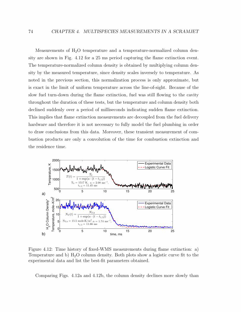
74 CHAPTER 4. MULTISPECIES MEASUREMENTS IN A SCRAMJET
Measurements of H2O temperature and a temperature-normalized column den-
sity are shown in Fig. 4.12 for a 25 ms period capturing the flame extinction event.
The temperature-normalized column density is obtained by multiplying column den-
sity by the measured temperature, since density scales inversely to temperature. As
noted in the previous section, this normalization process is only approximate, but
is exact in the limit of uniform temperature across the line-of-sight. Because of the
slow fuel turn-down during the flame extinction, fuel was still flowing to the cavity
throughout the duration of these tests, but the temperature and column density both
declined suddenly over a period of milliseconds indicating sudden flame extinction.
This implies that flame extinction measurements are decoupled from the fuel delivery
hardware and therefore it is not necessary to fully model the fuel plumbing in order
to draw conclusions from this data. Moreover, these transient measurement of com-
bustion products are only a convolution of the time for combustion extinction and
the residence time.
0 5 10 15 20 25500
1000
1500
2000
Tem
pera
ture
, K
Experimental Data
Logistic Curve Fit
0 5 10 15 20 250
5
10
15
20
time, ms
H2O
Colu
mn D
ensity*
Tem
pera
ture
, m
ole
−K
/m2
Experimental Data
Logistic Curve Fit
T (t) =T0
1 + exp(a · (t − t1/2))T0 = 1517 K, a = 2.08 ms−1,
t1/2 = 11.45 ms
NT (t) =NT,0
1 + exp(a · (t − t1/2))
NT,0 = 15.5 mole-K/m2, a = 1.74 ms−1,t1/2 = 11.66 ms
a)
b)
Figure 4.12: Time history of fixed-WMS measurements during flame extinction: a)Temperature and b) H2O column density. Both plots show a logistic curve fit to theexperimental data and list the best-fit parameters obtained.
Comparing Figs. 4.12a and 4.12b, the column density declines more slowly than

4.4. RESULTS 75
the temperature, identifying differences between thermal and mass transport in the
cavity. This result has never been observed before to our knowledge. A steady tem-
perature near 1500 K was observed near the 10 ms time in the plot, which then rapidly
declined to a steady value of about 650 K, indicating complete flame extinction as
this value is slightly lower than the static temperature of the inlet gas flow (perhaps
due to expansion effects in the cavity, however temperature measurements after flame
extinction suffer from a low signal-to-noise ratio due to the small amount of H2O in
the flow). A logistic function of the form 1/ (1 + e−x) was fit to the temperature
data (shown in Fig. 4.12a), and yields a time of 2.8 ms for the temperature to drop
from 5% to 95% of the total temperature range over the test. However, temperature
measurements may not be the best indicator of residence time because heat transfer
from products to the combustor walls and the bath gas will complicate the inter-
pretation of the temperature time-history. Measurements of temperature-normalized
column density offer fewer complications because once the flame is extinguished, the
production of new combustion product H2O rapidly ceases and the normalization
eliminates most of the influence of temperature on detecting transport of products
from the cavity. However, note that these measurements do not correct for variations
in pressure, which occur during flame extinction and will affect column density. H2O
column density measurements corrected for the changing temperature observed are
shown in Fig. 4.12b, and maintain a steady value of about 15.5 mole-K/m2 for a short
period after the temperature begins declining. However, after the 11 ms mark, the
column density begins to rapidly decline, ultimately to a steady value of about 0.98
mole-K/m2. Also shown in Fig. 4.12b is a logistic curve fit to the measurement data
with fitting parameters shown in the figure. The column density logistic fit yields a
time of 3.4 ms to drop from 5% to 95% of the total column density range over the test.
This value is 20% larger than the measured temperature time to decline, which rein-
forces the conclusion that there may be some significant differences between thermal
and mass transport in the cavity.
Because these measurements occurred during a flame extinction event, the mea-
sured times for combustion products in the cavity are limited by either the extinction
event time, the residence time in the cavity, or a convolution of both effects. If the

76 CHAPTER 4. MULTISPECIES MEASUREMENTS IN A SCRAMJET
flame extinction contributes to the measured time for combustion products to disap-
pear, then the cavity residence time must be shorter than the measurements presented
here. Thus, these measurements place an upper bound on the cavity residence time.
Future work may refine this technique to decouple flame extinction and residence time
effects and provide direct measurements of cavity residence time. However, note the
results presented here are consistent with CFD calculations of residence time based
on similar combustor geometries (around 2.3 ms for 5% to 95% of the total dynamic
range), and therefore this technique represents a valuable starting point in this new
application of laser absorption spectroscopy [118].

Chapter 5
Hypersonic Scramjet Combustor
Measurements Within a Reflected
Shock Tunnel
There is substantial interest in air-breathing hypersonic propulsion systems capable of
operating at flight speeds in the range of Mach 8-15 [16]. Vehicles operating at these
conditions would be fueled by liquid hydrogen and may be used for either manned
hypersonic cruising or for single-stage to orbit space vehicles [119]. At these flight
speeds, the flow within the combustor is hypersonic rather than just supersonic as it
was for the results presented in Chapters 3 and 4. This presents many challenges to
combustor design, chief among which is that fuel-air mixing is not well understood
at high Mach numbers where the bulk flow velocity is approximately equal to the
injector flow speed [120]. In order to better understand hypersonic combustion pro-
cesses, reflected shock tunnels have been commonly used to generate hypervelocity
conditions and test scramjet combustors at conditions equivalent to flight speeds of
Mach 10 or higher [121]. While model scramjet combustors used in these types of fa-
cilities commonly include instrumentation such as pressure transducers and heat flux
gauges, additional diagnostics are needed, particularly to determine temperature and
composition of species in the combustor [51, 122]. Optical sensors utilizing tunable
diode laser absorption spectroscopy (TDLAS) are an attractive source of temperature
77

78 CHAPTER 5. TDLAS IN A HYPERSONIC SCRAMJET COMBUSTOR
and H2O measurements in these facilities, as they offer both mechanical reliability as
well as fast time-resolution needed for measurements in a reflected shock tunnel.
Historically, tunable diode laser absorption spectroscopy (TDLAS) sensors have
played a pivotal role in characterizing hypersonic scramjet ground test facilities by
supplying in situ measurements of important thermophysical properties such as tem-
perature, species concentration, and velocity of the free-stream flow to better under-
stand test times and test gas contamination [51, 123–125]. More recently, researchers
have begun to apply TDLAS diagnostics to measure temperature and water vapor for
tracking combustion progress within model scramjet combustors during hypersonic
testing [80, 92]. However, these past studies have assumed that the conditions were
uniform along the line-of-sight (LOS) in their data reduction methods, and the flow
within hypersonic combustors is known to be highly three-dimensional [120]. Here we
acknowledge nonuniformity along the the LOS, but use a new scanned wavelength-
modulation spectroscopy (WMS) strategy to measure changes to the transition line-
shape due to nonuniformity and provide quantitative WMS absorption results [82, 84].
This work represents one of the first practical implementations of this new tech-
nique in a scramjet engine [126]. Scanned-WMS measurements are an important new
tool for characterizing scramjet combustion or any other flow where nonuniformi-
ties are present and the noise-rejection capabilities of WMS are desired. The sensor
probed two H2O absorption transitions near 1.4 µm to measure H2O column density
and water-weighted temperature downstream of fuel injection across three LOSs in
a model scramjet at the HyPulse reflected shock tunnel facility at ATK General Ap-
plied Science Laboratory (GASL) in Ronkonkoma, New York. Implementation of this
sensor presented several design challenges in delivery of light across multiple LOSs on
a model scramjet inside a pressure vessel. A detailed description of the facility and
TDLAS sensor hardware is included. Measurement results are presented from three
separate tests: one non-combusting mixing case and H2-air combustion at two unique
angles of attack and fuel-air equivalence ratio combinations.

5.1. HARDWARE DESCRIPTION 79
5.1 Hardware Description
5.1.1 ATK HyPulse Test Facility
Tests were performed on the NASA HyPulse facility, operated by ATK-GASL in
Ronkonkoma, New York at conditions equivalent to Mach 10 flight. HyPulse was
operated in reflected-shock-tunnel mode; a detonable H2/O2/Ar driver mixture ini-
tialized propagation of a shock through the test gas (N2 or air) over the length of
the 15.2 cm diameter tube, shock heating the test gas. The shock reflected off the
end-wall and propagated back upstream, stagnating and further shock-heating of the
test gas. This shock-heated air at the end-wall was the plenum for a hypersonic noz-
zle that accelerated flow into a large test cabin (diameter = 2.1 m). Here, the flow
was captured by a model scramjet forebody, inlet, and combustor, shown in Fig. 5.1.
The model inlet and combustor was machined from a solid block of aluminum and
the forebody from stainless steel. Because this is an impulse facility no cooling of the
model was necessary.
Fuel injector ramp
TDLAS hardware
with protective
cover plates
TDLAS @
x = 27.6 cm x = 0
Figure 5.1: Rendered view of inlet and combustor model used for Mach 10 scramjettesting at ATK HyPulse. Note the fuel injector ramp seen through large diagnosticwindows and TDLAS hardware 27.6 cm aft of the injector ramp. Forebody not shown.Wedged cover plate shown removed for visibility of TDLAS system.
Hydrogen fuel was injected into the captured flow at the base of a 10◦ unswept

80 CHAPTER 5. TDLAS IN A HYPERSONIC SCRAMJET COMBUSTOR
compression ramp (height H = 6.4 mm). As shown in the flow path diagram in Fig.
5.2, beginning 6.3 cm behind the injector ramp, the flow path diverged at an angle of
2.9◦ until exiting at the end of the rig (30.2 cm downstream of fuel injection). Three
separate sets of windows offered optical access to the flow path inside the scramjet.
Large viewing windows centered around the injector ramp were used for Schlieren
imaging. TDLAS measurements were made through windows 27.6 cm downstream
of fuel injection with clear aperture of 2.8 cm (height) by 0.64 cm (along flow path).
Here the duct height was 3.6 cm and the span between TDLAS LOS 1 (lower) and
LOS 3 (upper) was 2.3 cm. The LOS path length spanned 3.81 cm across the flow
path. Other instrumentation on the model included piezoelectric pressure transducers
and thin-film resistance and coaxial thermocouple heat flux gauges [127].
27.6 cm Flow
3 TDLAS LOS
2.3 cm
Figure 5.2: Drawing of model scramjet flow path, with three TDLAS measurementlocations noted.
5.1.2 TDLAS Sensor Layout
Figure 5.3 shows a diagram view of the the TDLAS hardware used in the sensor.
Signal generation, data acquisition, and laser hardware were all located outside of the
test cabin. Two lasers were used to probe H2O absorption transitions near 1391.7 nm
and 1469.3 nm. Note these were the same transitions as used in the Mach 5 H2-air
combustion tests presented in Chapter 3, and therefore for a discussion of line selection
the reader is referenced to Section 3.1.2. Sinusoid waveforms to scan and modulate
the laser injection current were generated digitally with a desktop computer; the scan
rate was 1 kHz and modulation was at 160 kHz and 200 kHz for the lasers near 1391.7
nm and 1469.3 nm, respectively. The fiber-coupled output light from the two lasers
was multiplexed onto one 9 µm core single-mode fiber and the combined signal was

5.1. HARDWARE DESCRIPTION 81
then split onto two separate single-mode fibers. A wall feed-through allowed both
fibers to be routed inside the test cabin where the fiber-coupled light was split again
to give a total of three fibers, each bringing light to a separate LOS. All three fibers
were routed to the scramjet model where they were attached to collimating optics
to transmit light on three measurement LOSs. On the opposite side of the model,
light was turned 90◦ by mirrors and collected by focusing lenses and routed onto 600
micron multi-mode fibers to an adjacent metal box containing detection hardware.
The output light from each fiber was focused onto a detector (Thorlabs PDA10CS)
by doublet lenses. Detectors had a bandwidth of 17 MHz, which was anti-aliasing
filtered to 1 MHz. The detector signal was routed out of the tunnel on BNC cables,
through BNC wall-feedthroughs, and back to a computer for data acquisition at a
rate of 10 MHz, with 12-bit resolution over a 2 V dynamic range. All cabling within
the test cabin was enclosed in 1.25 cm or 2.5 cm diameter steel-reinforced hosing
to protect it from the hypersonic flow from the expansion nozzle. The metal box
enclosing the detectors protected that hardware.
The optical system mounted on the model scramjet, shown in Fig. 5.4, had three
parallel LOSs spaced evenly by 1.15 cm, spanning 2.3 cm. Fig. 5.5 shows dashed
lines and labels depicting all three TDLAS measurement LOSs, numbered “LOS 1,”
“LOS 2,” and “LOS 3.” LOS 1 was 0.15 cm from the injector wall, LOS 2 was 1.30
cm from the injector wall, and LOS 3 was 2.45 cm from the injector wall (or 3.45
cm, 2.3 cm, and 1.15 cm from the top of the flow channel, respectively). All three
LOSs were 27.6 cm downstream of fuel injection. Adjacent optical LOSs alternated
between transmission and receiving on each side of the combustor in order to allow
this compact spacing arrangement. The optical mounting system consisted of a large
plate with a rectangular hole in the center used as an interface between the optics and
the model combustor. Optics were attached to a second, smaller, plate that sat away
from the large plate on 2.5 cm spacers. Each LOS was individually adjustable over one
translational and two rotational degrees of freedom. Vertical translation was allowed
by mounting each optical element on dovetail brackets that were clamped into their
final position by a bolt and washer. As shown in Fig. 5.6, the optics themselves were
attached to a second piece floating below the bracket on several bolts with a set screw

82 CHAPTER 5. TDLAS IN A HYPERSONIC SCRAMJET COMBUSTOR
+ +
+ +
Slow scan
1 kHz
+++
++++++ Fast scan
200 kHz
160 kHz
1392 nm 1469 nm
Fiber
Combiner/
Splitter
Single-Mode Fiber
Computer
Detectors
Air
Flow
Detector Signals
Test Cabin
Fiber-Wall
Feedthrough
sss
Protective Box
Multi-Mode
Fiber
Figure 5.3: Diagram of TDLAS hardware layout for ATK HyPulse measurements.
acting as a fulcrum. By tightening the bolts to varying degrees, adjustments could
be made in two axes of rotation about the fulcrum. Because each optical element
could be individually adjusted and locked in position, optimizing alignment of light
across the flow path in the model proved fairly simple, and this alignment was robust
through multiple facility operation cycles.
Light was transmitted across the combustor on each LOS using a 3.8 mm diameter
fiber-coupled GRIN (gradient-index) lens (OZ Optics). On the receiver side the light
was first turned parallel to the flow path with a 5 mm right-angle mirror, and then
was collected on a 10 mm diameter ThorLabs F240SMA-C aspheric lens to couple
the transmitted light onto the collection fiber. The large collection optic diameter
ensured complete light collection in the presence of beam steering due to density
gradients that can skew the LOS. The entire optical assembly was protected from the

5.2. RESULTS 83
Fore and aft TDLAS windows
(Only aft used in experiments)
LOS
“Pitch” Lens
“Catch” turning mirror
and collection lens
Set screws for
alignment
adjustment a) b)
Interface Bracket
Window Optics
Bracket
Rear Cover
Plate with
Fiber Routing
Figure 5.4: Detailed view of TDLAS hardware attached to HyPulse model combustor.a) Rendered view b) Photograph
hypersonic flow with a two-piece steel wedged cover plate. A rear cover plate was
threaded to accept the protective cabling (shown in Fig. 5.4b), allowing all fibers
to be routed to the optics and complete access to adjustment screws while mounted
to the model. A three-sided wedge-shaped cover plate was then bolted over the rest
of the optics to completely protect them from the oncoming flow. The edges of the
entire assembly were sealed with aluminum tape to minimize leaking of the test gas
into ambient optical path during the test.
5.2 Results
TDLAS results from three Mach 10 tests will be presented here. First, raw WMS-
2f /1f signals are presented and qualitative results are discussed. Next, quantitative
results are shown, beginning with column density measurements from a tare run with-
out combustion in the model. Then column densities and temperatures of two com-
bustion cases are presented, the first at an angle of attack of θ = 1◦ and hydrogen-air
equivalence ratio of Φ = 1.31 and the second at angle of attack of θ = 7.5◦ and equiv-
alence ratio Φ = 1.03. The flow conditions for all three runs are summarized in Table
5.1. Results are shown as time-histories with the abscissa in milliseconds and TDLAS

84 CHAPTER 5. TDLAS IN A HYPERSONIC SCRAMJET COMBUSTOR
Pressure transducer
LOS 1
LOS 2
LOS 3
Figure 5.5: Cross section view of TDLAS hardware with LOS labeling.
Dovetail
Bracket
5 mm 90° Turning Mirror
Fulcrum Bolts Adjust
Angle and Lock
in Place
Figure 5.6: Detailed view of dovetail bracket and 90◦ turning mirror holder (holdertranslucent for visualization). A single set screw in the center acts as a fulcrumagainst the three bolts threaded into the mirror holder, allowing for two rotationaldegrees of freedom.
measurements reported every 0.5 ms (2 measurements per 1 kHz scan). The time ori-
gin is defined by the arrival of the test gas at the measurement location and the 3 ms
test window was defined based upon the steady duration of pressure traces from the

5.2. RESULTS 85
Table 5.1: Experimental flow conditions within the model scramjet combustor foreach of three tests conducted at ATK HyPulse.
Angle ofattack,
deg.Test gas
EquivalenceRatio, Φ
Free-streamtemperature,
K
CombustorPressure, atm
MachNumber
1 N2 N/A 1180 0.302 4.141 air 1.31 1180 0.302 4.14
7.5 air 1.03 1477 0.475 3.5
model collected upstream of the TDLAS measurement. The beginning and end of the
test window is marked on each plot. Results were calculated using the scanned-WMS
methodology discussed in Section 2.3.2. Due to the unsteady conditions in these
measurements, the differences between measurement error and flow field fluctuation
are difficult to quantify. Estimated measurement uncertainty includes errors of about
1.5% in temperature and column density measurements, based on heated static-cell
experiments at known conditions conducted at Stanford University [82] and similar
measurements in a continuous-flow Mach 5 model scramjet combustor (See Chapter
3). The sensors used to estimate the uncertainty employed the same absorption tran-
sitions and similar measurement techniques. These other measurements had errors of
less than 1% when compared to facility conditions. However, this estimate does not
account for additional facility flow field noise and rapid transients, and hence to be
conservative the uncertainty estimated here is larger.
5.2.1 Normalized WMS-2f Signals
Because of the robust and high signal-to-noise ratio of the data acquired, a qualitative
understanding of the flow-physics is obtained by examining the raw WMS data. Fig-
ure 5.7 shows measured WMS-2f /1f signals for the absorption transition at 1391.7
nm over each of the three tests before, during, and after the steady test time. Note
that for each test, the laser wavelength scan is not synchronous with the facility test
trigger and hence the timing of absorption signals relative to the test time varies in
each experiment. Data was acquired for all tests for 1.5 ms before the arrival of the
test gas, however only about 0.75 ms of data is shown before the test gas arrival to

86 CHAPTER 5. TDLAS IN A HYPERSONIC SCRAMJET COMBUSTOR
account for data buffering in the digital low-pass filter. Figure 5.7a shows measured
signals for the non-combusting measurements. The first millisecond shows no strong
absorption signals despite test gas arrival at 0 ms. Although there is a spike in the
signal near 1.4 ms, the shape of this feature is not consistent with the characteristic
three-lobe WMS-2f /1f lineshape from absorption, and it is believed to be caused
by interference from debris in the flow blocking a portion of the beam. The first
WMS-2f /1f lineshape from absorption is observed at approximately 1.8 ms after test
gas arrival, when only driven N2 should be present in the measurement region. This
well-defined lineshape is interpreted as evidence of H2O present in the combustor.
Subsequently, the measured absorption signal increased in magnitude throughout the
remainder of the test. This behavior is consistent with increasing H2O concentration
in time at constant temperature. Because no absorption was observed in measure-
ments between -0.75 ms and 1.8 ms, the rise in H2O concentration versus time must
be from mixing of driver (H2 and O2 combustion products and Ar) and driven gas
(N2 for the non-combusting case and air for combustion cases) in the facility. The
penetration of driver gas into the test gas in shock-driven hypersonic test facilities
is well known [128–132], although the measurements reported here are perhaps the
most sensitive yet made (H2O mole fraction at 2 ms of about 1.5%).
The combustion cases shown in Figs. 5.7b and 5.7c tell two different stories:
the first indicates almost no combustion until the test time was nearly over and the
second shows strong evidence of combustion even before the steady test time began.
A low angle of attack, high equivalence ratio case shown in Fig. 5.7b shows no strong
absorption signals until 1.8 ms after the arrival of the test gas. Only weak absorption
is observed until about 4 ms, indicating very limited combustion up to this point.
After 4 ms, the absorption signal doubled, indicating sudden combustion initiation
near the end of the steady test time. The signal in Fig. 5.7c, however, shows fairly
strong H2O absorption signals beginning immediately after the test gas arrival. The
larger angle of attack produces higher enthalpy flow conditions in the combustor,
thereby promoting ignition. By the beginning of the test time, absorption signals
were significantly stronger than the corresponding absorption observed during the
mixing case, indicating a significant presence of H2O due to combustion.

5.2. RESULTS 87
0 1 2 3 4 5 60
0.05
0.1
0.15
0.22
f/1
f S
ign
al
0 1 2 3 4 5 60
0.1
0.2
Time, ms
2f/
1f
Sig
na
l
Test Gas
Arrival
2
Begin Test
Time End Test
Time
a)
b)
c)
Signal interference
due to beam blockage
0 5
0 1 2 3 4 5 60
0.05
0.1
0.15
0.2
2f/
1f
Sig
na
l Background Signal
Background-subtracted Measured Signal
Figure 5.7: Measured 1f -normalized WMS-2f signals before, during and after testtime on absorption feature at 1391.7 nm over LOS 3: a) Non-combusting mixingcase, b) Combustion with angle of attack θ = 1◦, equivalence ratio Φ = 1.31, c)Combustion with angle of attack θ = 7.5◦, equivalence ratio Φ = 1.03. In each case,fuel flow was initiated at the beginning of TDLAS data acquisition, 1.5 ms before thearrival of the test gas.
These conclusions based on raw WMS-2f signals are in good agreement with
axial pressure measurements to detect combustion onset, shown in Fig. 5.8. In the
mixing case, there is a moderate pressure rise over the test time consistent with
fuel injection, but not combustion. The low angle of attack, high equivalence ratio
case initially shows only a gradual pressure rise similar to the mixing case, followed
by a significant pressure rise around t = 4 ms due to combustion. At the higher
angle of attack there is an immediate pressure rise, indicating prompt combustion.
Also shown in Fig. 5.8d are the pressure time-histories at the TDLAS measurement
location (134.6 cm downstream of the forebody leading edge) over each of the three
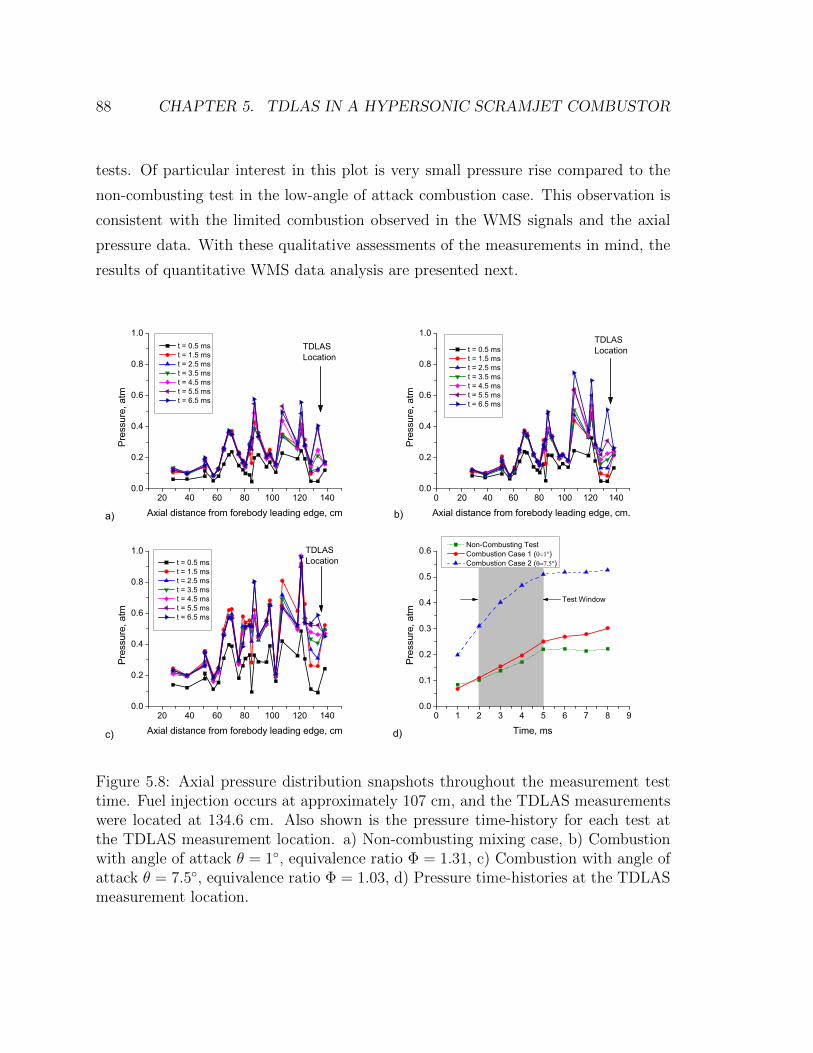
88 CHAPTER 5. TDLAS IN A HYPERSONIC SCRAMJET COMBUSTOR
tests. Of particular interest in this plot is very small pressure rise compared to the
non-combusting test in the low-angle of attack combustion case. This observation is
consistent with the limited combustion observed in the WMS signals and the axial
pressure data. With these qualitative assessments of the measurements in mind, the
results of quantitative WMS data analysis are presented next.
20 40 60 80 100 120 1400.0
0.2
0.4
0.6
0.8
1.0
Pres
sure
, atm
Axial distance from forebody leading edge, cm
t = 0.5 ms t = 1.5 ms t = 2.5 ms t = 3.5 ms t = 4.5 ms t = 5.5 ms t = 6.5 ms
a)
TDLASLocation
0 20 40 60 80 100 120 1400.0
0.2
0.4
0.6
0.8
1.0
Pres
sure
, atm
Axial distance from forebody leading edge, cm.
t = 0.5 ms t = 1.5 ms t = 2.5 ms t = 3.5 ms t = 4.5 ms t = 5.5 ms t = 6.5 ms
b)
TDLASLocation
20 40 60 80 100 120 1400.0
0.2
0.4
0.6
0.8
1.0
Pres
sure
, atm
Axial distance from forebody leading edge, cm
t = 0.5 ms t = 1.5 ms t = 2.5 ms t = 3.5 ms t = 4.5 ms t = 5.5 ms t = 6.5 ms
c)
TDLASLocation
0 1 2 3 4 5 6 7 8 90.0
0.1
0.2
0.3
0.4
0.5
0.6
Pres
sure
, atm
Time, ms
Non-Combusting Test Combustion Case 1 ( ) Combustion Case 2 ( )
d)
Test Window
Figure 5.8: Axial pressure distribution snapshots throughout the measurement testtime. Fuel injection occurs at approximately 107 cm, and the TDLAS measurementswere located at 134.6 cm. Also shown is the pressure time-history for each test atthe TDLAS measurement location. a) Non-combusting mixing case, b) Combustionwith angle of attack θ = 1◦, equivalence ratio Φ = 1.31, c) Combustion with angle ofattack θ = 7.5◦, equivalence ratio Φ = 1.03, d) Pressure time-histories at the TDLASmeasurement location.

5.2. RESULTS 89
5.2.2 Non-combusting Test
In the non-combusting test, nitrogen replaced air as the test gas of the shock tube so
that fuel could be injected into the scramjet without combustion and mixing of the
driver gas and test gas could be evaluated. The shock tube driver was a stoichiometric
mixture of H2 and O2 diluted in 30% Ar, and H2O combustion products were formed
by the driver detonation. If the test gas and driver had been un-mixed in the shock
tube, the TDLAS sensor would begin to detect H2O at the end of the test gas flow
and the beginning of the driver gas. However, early arrival of H2O could signal mixing
of the test and driver gases before the expansion nozzle. Therefore, TDLAS measure-
ments of H2O in this test case aimed to track the arrival of the driver gas. This test
also served as a validation of the TDLAS hardware to maintain optical alignment and
mechanically survive the harsh conditions experienced in this facility. The gas was
too cool and H2O concentration was too low to maintain strong absorption for the
feature at 1469.3 nm. However, the feature at 1391.7 nm maintained strong absorp-
tion in these conditions, as evidenced by the measured time-series of the WMS-2f /1f
signal shown in Fig. 5.7a, discussed previously. Because absorption on the 1469.3 nm
feature was so weak, the conventional two-line thermometry approach was discarded
to reduce the propagation of temperature uncertainty into column density measure-
ments. Instead, 1-D shock-jump and isentropic relations were used in conjunction
with the known total and static conditions out of the facility nozzle to calculate the
temperature downstream of the combustor to be 1158 K. This temperature was used
in conjunction with the absorption signal from the feature at 1391.7 nm to determine
column density. Additionally, it should be noted that this measured column density
solution is not strongly dependent on the temperature solution – the column density
sensitivity to temperature is 6% per 100 K at these conditions.
The resulting plot of column density, shown in Fig. 5.9, reveals early arrival of
H2O. This result is consistent on all three LOSs and H2O is seen throughout the test
window, increasing up to a maximum of 0.075 g/m2 at 5 ms. This value corresponds
to about 5.3% H2O by mole, which is 20 times larger than the sensor detection
limit based on minimum signal levels required at these conditions. The mixing of
driver gas into the test gas in reflected shock tunnels is a well-known phenomenon,

90 CHAPTER 5. TDLAS IN A HYPERSONIC SCRAMJET COMBUSTOR
-2 0 2 4 6 8 10 12 14 16 18 20
0.0
0.1
0.2
0.3
0.4
0.5
Col
umn
Den
sity
, g/m
2
Time, ms
LOS 1 LOS 2 LOS 3
Test Window
Figure 5.9: TDLAS column density measurements from Mach 10 non-combustingtare test case.
occurring due to boundary-layer “jetting” as the reflected shock propagates through
the shock tube [124, 133]. While the presence of driver gas has a minimal effect on
the gas-dynamic flow properties in this facility due to the similarity of the driver
γ with that of the test gas [132], it will alter combustion chemistry and thus this
TDLAS measurement of the driver gas concentration provides an important input for
modelers attempting to compare their results with facility measurements. Previous
measurements at these conditions have estimated that driver gas did not appear in
the test gas until approximately 3.5 ms after the arrival of the test gas [132]. Our
measurements confirm that finding at levels of approximately 2% H2O by mole at
t = 3.5 ms. In addition, because of better SNR of the scanned-WMS TDLAS sensor,
we also report smaller concentrations of driver gas in the test gas at even earlier times
in the test window.

5.2. RESULTS 91
5.2.3 Hydrogen-Air Combustion (θ = 1◦, Φ = 1.31)
The first of two combustion tests was conducted at an angle of attack of θ = 1◦
with H2-air equivalence ratio Φ = 1.31. Results for this test are shown in Fig. 5.10.
Steady-state CFD computation results along the three TDLAS LOSs are shown as
matching line-style arrows on the ordinate axis of each plot. The CFD is based upon
the work in [134], but with pure hydrogen fuel to match the test condition. CFD
column density was computed by direct evaluation of Eq. (2.7), and temperature
is the H2O-weighted average along the LOS, as given by (2.5). Column density
results are given in Fig. 5.10a. At the beginning of the test window there are many
similarities to results from the non-combusting case, with relatively small column
density observed. However, after t = 3 ms the column density jumps up drastically,
and by the end of the steady test time, measurements are equivalent to 15.0% H2O by
mole, providing clear evidence of ignition. However, complete, uniform combustion
would correspond to a column density of about 0.28 g/m2 and peak column densities
over the test window are only about two-thirds of this value, indicating combustion
is incomplete. CFD calculations agree almost exactly with peak measurement results
on LOS 2, however measurements on LOSs 1 and 3 are about 30% smaller than the
CFD values. This indicates that the measurements show less-complete combustion
than CFD predicts.
Temperature results in Fig. 5.10b do not show values before t = 3 ms, as the
absorption signal was too weak to confidently determine temperature. All tempera-
ture measurements over the test window show a significant temperature rise over the
static temperature based on 1-D calculations, confirming heat release from combus-
tion. The results are also in reasonable agreement with CFD, with peak temperature
values during the test time within 6%, 5%, and 16% for LOS 1, 2, and 3 respectively.
LOS 1 and LOS 2 are mostly lower than CFD predictions and LOS 3 is mostly higher
throughout the test time. These results indicate some combustion, but that CFD once
again tends to over-estimate the extent of combustion at the TDLAS measurement
location. At very late times after the test window (t = 8 − 18 ms) the temperature
drops uniformly on all three LOSs as the driver gas cools and expands through the
test cabin.

92 CHAPTER 5. TDLAS IN A HYPERSONIC SCRAMJET COMBUSTOR
-2 0 2 4 6 8 10 12 14 16 18 200.00
0.05
0.10
0.15
0.20
0.25
0.30
0.35
0.40
0.45
0.50
CFD
Test Window
Col
umn
Den
sity
, g/m
2
Time, ms
LOS 1 LOS 2 LOS 3
Approx. H2O forcomplete combustion
a)
Driver combustion products
-2 0 2 4 6 8 10 12 14 16 18 200
500
1000
1500
2000
Tem
pera
ture
, K
Time, ms
LOS 1 LOS 2 LOS 3
Test Window
b)
Static T
CFD
Figure 5.10: TDLAS results for Mach 10 combustion case θ = 1◦, Φ = 1.31 com-pared with steady-state CFD solutions. a) H2O column density b) H2O-averagedtemperature
5.2.4 Hydrogen-Air Combustion (θ = 7.5◦, Φ = 1.03)
Results for the second combustion test at angle of attack θ = 7.5◦ and equivalence
ratio Φ = 1.03 are shown in Fig. 5.11. This higher angle of attack was chosen for the
higher static temperature it would achieve in the combustor (1477 K) in an effort to
promote ignition. Once again, values from steady CFD calculations for each LOS are
shown as matching line-style arrows along the ordinate axis. Column density results
in Fig. 5.11a show significant concentration of combustion products even before the
test time begins, suggesting prompt ignition at this higher static temperature. Near
the end of the steady test time, these results are in fairly good agreement with the
steady-state CFD. Peak measurements at LOSs 1 and 2 are within 10% of the CFD
values, but LOS 3 measurements are more than 25% higher than the CFD prediction.
There are also significant point-to-point fluctuations in the data values. Some of this
variation, particularly at LOS 3 which is farthest from fuel injection in the flow, may
be because H2O does not penetrate as far into the flow as given by CFD simulation.
Peak column density measurements over the test time are also lower than the expected
uniform-flow column density of about 0.6 g/m2 for complete combustion, indicating
combustion has not proceeded to completion. Measurements of temperature in Fig.

5.2. RESULTS 93
5.11b show only a small rise over the static temperature, which gives credit to the
notion of limited combustion progress. Moreover, these results are in reasonable
agreement with the CFD values, although once again CFD appears to over-predict
the temperature slightly. However, peak temperature measurements are generally
about 15% higher than CFD predictions and occur sporadically, which may indicate
the presence of temporary “pockets” of hot combustion products passing along the
LOS. Temperature measurements do not have the monotonic decrease after the test
time, as observed in the first combustion test, however a general trend of declining
temperature can be seen. In both combustion tests, the temperature and column
density appear to be related inversely; the column density rises over the test time
while the temperature decreases. At first this result may seem counter intuitive,
but in addition to column density increasing due to combustion progress, column
density scales like all density measurements – proportional to pressure and inverse
to temperature. Therefore, one interpretation of these measurements (though not
the only one, given the complex flow physics) is that the density of the gas increases
during the test time since the pressure rises (see Fig. 5.8c) and temperature falls,
which in turn leads to larger values of column density.
-2 0 2 4 6 8 10 12 14 16 18 200.0
0.1
0.2
0.3
0.4
0.5
H2O ~0.6 g/m2 forcomplete combustion
Col
umn
Den
sity
, g/m
2
Time, ms
LOS 1 LOS 2 LOS 3
Test Window
a)
CFD
-2 0 2 4 6 8 10 12 14 16 18 200
200400600800
10001200140016001800200022002400
Tem
pera
ture
, K
Time, ms
LOS 1 LOS 2 LOS 3
Test Window
b)
CFD
Static T
Figure 5.11: TDLAS results for Mach 10 combustion case θ = 7.5◦, Φ = 1.03 com-pared with steady-state CFD solutions. a) H2O column density b) H2O-averagedtemperature

Chapter 6
Shock Tube Demonstration of a
Temperature Sensor for High-T
and -P Air Using NO Absorption
As evidenced by the preceding chapters, hypersonic aeropropulsion facilities rely on
high-enthalpy air as a critical input for operation. These facilities simulate supersonic
flight conditions by heating and pressurizing air for enthalpy matching prior to nozzle
expansion to high gas velocities. Enthalpy limitations in such facilities have been in
part attributed to difficulties in controlling or modeling the heating process such that
the enthalpy condition in the preheater is not well known at high temperatures (T >
2000 K) [135]. This challenge is exacerbated by a lack of options for directly measuring
gas temperature above the limits of conventional thermocouple materials, which melt
or oxidize at such extreme conditions. Alternative thermometry techniques are needed
for system evaluation and quantitative control feedback. Here we propose and validate
a spectroscopic strategy to measure temperature in high enthalpy air (T = 1200 - 3000
K) by probing the infrared absorption spectra of nitric oxide (NO).
Nitric oxide is selected amongst the species in high-temperature air due to the
sensitivity of its relative concentration to temperature at chemical equilibrium and
the strength of the vibrational absorption bands of NO in the infrared domain wherein
tunable, coherent light sources are readily available. For this work, the fundamental
94

6.1. MEASUREMENT METHODS 95
band near 5.2 µm is probed using a quantum cascade laser system. Key spectroscopic
parameters were measured in controlled thermodynamic environments to build a Voigt
lineshape spectral model, and the model was assessed at high gas densities (∼20
Amagat) in an optical cell. Fixed-wavelength direct absorption measurements were
conducted in non-reactive shock tube experiments to measure gas temperature over
a range of high enthalpy conditions (T = 1100 - 2950 K, P = 12 - 145 atm) with
known concentrations of NO in nitrogen. Lastly, the technique was demonstrated to
measure temperature in air at equilibrium behind reflected shock waves.
6.1 Measurement Methods
6.1.1 Chemical Equilibrium
Due to the temperature dependence of the composition of air in chemical equilibrium,
a measurement of nascent species concentration can be used to infer temperature. The
equilibrium composition of neat air (79% N2, 21% O2) is shown in Fig. 6.1 from 800 -
3000 K at 50 atm. Over this temperature range, diatomic nitrogen (N2) and diatomic
oxygen (O2) remain nearly constant, and the two most abundant minor species are
nitric oxide (NO) and atomic oxygen (O), which rise monotonically. The latter two
minor species present the greatest potential for equilibrium-based thermometry, and
serve as the primary candidates for spectroscopic sensing in the target temperature
domain. Other minor species such as nitrogen dioxide (NO2) and atomic nitrogen (N)
also have strong temperature sensitivity, but are present at much lower concentrations.
In higher temperature applications, such as arc heaters (T > 4000 K) laser absorption
sensing of nitrogen and oxygen atoms has been utilized to measure gas temperature
[136, 137]. Here nitric oxide is the target species for thermometry due to its relative
abundance from 1500 - 3000 K and convenient spectroscopic activity in the infrared.
The sensitivity of nitric oxide concentration to temperature and pressure in equi-
librium air is further illustrated in Fig. 6.2. As observed on this linear scale, the
mole fraction of NO changes by more than two orders of magnitude between 1200
K and 3000 K. Moreover, there is negligible pressure dependence between 15 atm

96 CHAPTER 6. HPST NITRIC OXIDE MEASUREMENTS
1000 1500 2000 2500 3000
0.001
0.01
0.1
1
Temperature [K]
Mole
Fra
ction
NO
O2
N2
O
P = 50 atm
Figure 6.1: Air in chemical equilibrium at 50 atm, T = 900 - 3000 K.
and 150 atm, which implies that over this domain mole fraction and temperature are
uniquely coupled. In the range of 2000 - 3000 K, a higher priority due to thermocou-
ple inadequacy, the equilibrium mole fraction ranges from 0.8% to 4.4%, which is an
appreciable quantity for sensing purposes. The strong dependence on temperature
leads to a sensitive thermometry technique, such that around 2300 K, a measurement
of mole fraction with 5% uncertainty would yield a measurement of temperature to
within 1% uncertainty.
An underlying assumption of the current approach to thermometry is that the gas
being probed is in chemical equilibrium, which requires time. Figure 6.3 provides a
kinetic analysis of the characteristic time required for NO to reach equilibrium when
forming from air at a given temperature. Similar characteristic times are observed
when air is being cooled after heating. These characteristic times can be compared
with residence times in the heater system to establish a lower bound to the tem-
perature at with the equilibrium-based strategy would be effective. For reference,
in stagnation conditions wherein the gas particle residence times are on the order of
seconds, the lower temperature bound would be 1700 - 2000 K, depending weakly

6.1. MEASUREMENT METHODS 97
1500 2000 2500 30000.00
0.01
0.02
0.03
0.04
0.05
1%NO
Mol
e Fr
actio
n
Temperature [K]
P = 15 bar P = 150 bar
5%
XNO(1200 K) = 200 ppm
Figure 6.2: Nitric oxide mole fraction in equilibrium air from 1200 to 3000 K at 15atm (black) and 150 atm (red).
on pressure and other processes like mixing. A more rigorous chemical kinetic anal-
ysis, unique to each gas system or heating process, is recommended to establish a
precise lower bound for a given application. Overall, the equilibrium-based assump-
tion is more reliable at higher temperatures, which is where the thermometry need is
greater.
6.1.2 Nitric Oxide Absorption Spectrum
Absorption spectroscopy is a well-established technique for non-intrusive gas sens-
ing. Numerous laser-based absorption diagnostics have been successfully utilized to
measure gas properties in harsh environments wherein conventional, more intrusive
sensors are less suitable [92, 111, 138, 139]. Moreover, absorption spectroscopy in the
infrared wavelength domain allows for the utilization of compact, room-temperature
semiconductor lasers, advantageous for applications outside of the laboratory. Figure
6.4 shows the infrared absorption spectra of nitric oxide at 2000 K over the wavelength
range of 1.5 - 7.5 µm. Previous work using tunable diode lasers for NO detection has

98 CHAPTER 6. HPST NITRIC OXIDE MEASUREMENTS
1500 2000 2500 3000
10-3
10-1
101
103 P = 50 atm P = 150 atm
[s]
Temperature [K]
Figure 6.3: Characteristic time required for NO to reach equilibrium when formingfrom neat air (79% N2, 21% O2).
been well-established in the overtone vibrational bands near 1.8 µm and 2.7 µm
[140, 141]. Falcone, et al. characterized many transitions in the fundamental band
spectrum of NO, however at the time these wavelengths were accessed by low-power
cryogenic tunable diode lasers, making field measurements impracticable [142]. The
more recent availability of quantum cascade lasers has further enabled practical field
sensing by probing the fundamental band of NO near 5.2 µm [143, 144]. Here the
fundamental absorption band was selected for its superior strength and potential for
sensitive detection of nitric oxide in high-enthalpy air.
Wavelength selection within the fundamental band relies on the relative strength
of the rotational transitions that comprise the band, as well as spectral isolation
from water vapor. Expected absorbance values are simulated using the Hitemp 2010
database [102], coupled with a Voigt lineshape model, to guide in wavelength selection.
The validity of this lineshape model is evaluated experimentally and discussed in a
later section. Figure 6.5 depicts the expected absorbance spectrum of the fundamental
band at 2000 K and 3000 K (P = 50 atm), highlighting the strength and temperature

6.1. MEASUREMENT METHODS 99
Figure 6.4: Infrared absorption linestrengths of nitric oxide at 2000 K from 1.5 - 7.5µm
sensitivity of NO absorbance in chemical equilibrium. It can be observed that the R-
branch (1890 - 2010 cm−1) is stronger and more isolated from water than the P-branch
(1700 - 1890 cm−1). A target wavelength was chosen near the peak of the R-branch
at 1927.3 cm−1, where water interference is minimal (<0.5%). To model water vapor
interference, it was assumed that the air is compressed near room temperature prior
to heating, and thus the majority of ambient moisture condenses out prior to the
temperature measurement. At a pressure of 25 atm, which is toward the lower end
of the target pressure range, moisture in humid ambient air would be reduced to
1000 ppm by such a process, which is the level simulated in Fig. 6.5. Further fixed-
wavelength simulations of absorbance as a function of temperature at 1927.3 cm−1
are shown in Fig. 6.6. The selected wavelength is near the peak of the R(15.5) line
of the Π3/2 electronic ground state, but at such pressures the absorbance at a fixed
wavelength includes contributions from several neighboring NO transitions.

100 CHAPTER 6. HPST NITRIC OXIDE MEASUREMENTS
1800 1900 20000.0
0.5
1.0
2000 K
P = 50 atmL = 10 cmXNO = XNO,eq
Absorba
nce
Wavenumber [cm-1]
3000 K
H2O
TargetWavelength
Figure 6.5: Simulated absorbance spectra of equilibrium nitric oxide near 5.2 µm at2000 K and 3000 K; water vapor also simulated at 2000 K, 1000 ppm; L = 10 cm
6.2 Measurement Results
6.2.1 Facility and Sensor Hardware
Measurements to characterize the NO spectrum in the region of the R(15.5) transition
near 1927.3 cm−1 and to demonstrate the sensor concept were performed in two
primary facilities: a high-pressure optical cell (see Ref. [145]) and the Stanford High
Pressure Shock Tube (HPST). The HPST facility consists of a 7.62 cm inner diameter,
3 m long driver section and a 5 cm inner diameter, 5 m driven section. Driver and
driven sections are separated by a diaphragm made either of aluminum or steel,
which is scribed to control the rupture [146]. Shocks are generated by filling the
driven section with a test gas (here, N2 and NO, or N2, O2, and N2O), then filling the
driver section with helium until the diaphragm bursts. There are five fast-response
piezo-electric pressure transducers (PCB Pl 13A) along the last 1.5 m of the driven
section of the shock tube, which trigger time-interval counters (Phillips PM6666)
as the incident shock passes over them. Using the known distances between the

6.2. MEASUREMENT RESULTS 101
1500 2000 2500 30000.0
0.5
1.0
1.5
2.0
(d / )/(dT/T)N
O A
bsor
banc
e
Temperature [K]
P = 50 atm P = 100 atm
1
L = 10 cmXNO = XNO,equilibrium
2
4
6
8
Temperature S
ensitivity
Figure 6.6: Simulated absorbance and temperature sensitivity at 1927.3 cm−1 from1400 - 3000 K; P = 50 atm (black) and P = 100 atm (red).
counters, the incident shock velocity was calculated and used to obtain the test gas
temperature behind the reflected shock using standard normal shock relations. This
method is generally accurate to within 0.7% [147].
A diagram of the NO sensor hardware is provided in Fig. 6.7. An external-
cavity quantum-cascade laser (ECQCL) from Daylight Solutions, emitting near 5.2
µm, provided light for the present experiments. The 50 mW beam was split using a 2-
degree wedged CaF2 window, directing a reference beam consisting of about 3% of the
total output light to a thermoelectrically-cooled Mercury-Cadmium-Telluride (MCT)
detector (Vigo). Recording this reference signal allowed normalization for common-
mode components of the laser signal, which significantly improved the sensor detection
limits [148]. After passing through the high-pressure cell or shock tube, the primary
beam was focused using a 10 cm focal-length CaF2 lens into a 2.54 cm diameter, gold
coated integrating sphere with 6.4 mm ports (Sphere Optics). The integrating sphere
provided decreased sensitivity to beam steering, which is particularly important due
to severe density gradients in the HPST [146]. Light diffusely reflects over the entire

102 CHAPTER 6. HPST NITRIC OXIDE MEASUREMENTS
Data Acquisition
Computer
EC QCL
5.2 µm
High-P Cell/Shock Tube
BeamsplitterCaF2 Lens
4.9 µm LP
Filter
Integrating
Sphere
Reference
Detector
Detector
Figure 6.7: Diagram of sensor hardware for NO measurements through a high-pressurecell and the Stanford High-Pressure Shock Tube.
surface of the integrating sphere, which provides a margin for error as the beam
can wander from its initial alignment without any significant change in the detector
signal [149]. However, when using an integrating sphere, the detector only samples a
fraction of the total light no larger than the ratio of the active area of the detector
to the total area of the sphere surface, which results in at least a 98% laser power
loss through the optical system. The output light from the integrating sphere was
filtered with a 4.9 µm long-pass spectral filter to mitigate any emission signal on the
detector. Additional spatial filtering was provided by irises at the shock tube exit
port and directly in front of the CaF2 focusing lens, but these components are not
shown in Fig. 6.7. Transmitted light was captured on a liquid-nitrogen cooled Indium
Antimonide detector with a 4 mm2 active area (InfraRed Associates). For shock tube
tests at fixed wavelength, the output wavelength was monitored using a standalone
high-accuracy wavelength meter (Bristol, not shown in Fig. 6.7).
6.2.2 Spectral Characterization
While databases of spectral parameters such as Hitemp [102, 150] provide a valuable
starting point for understanding spectral absorption of nitric oxide, these databases
are sometimes found to be inaccurate, particularly at very high temperatures where

6.2. MEASUREMENT RESULTS 103
they were not originally designed to be used. The quoted uncertainty in Hitemp for
the linestrength of the R(15.5) transition is 10% and the collision-width uncertainty at
1500 K is 15%. Therefore, in order for the proposed sensor to achieve quantitatively
accurate measurements at high-temperature and -pressure conditions, the NO absorp-
tion spectrum was characterized under controlled conditions. Two separate spectral
characterization and validation studies were conducted, both using controlled mix-
tures of NO in N2 balance. First, NO absorption was measured across a range of
pressures to assess whether the Hitran database using a Voigt lineshape model would
accurately represent the NO spectrum at high densities. Next shock tube measure-
ments characterize the temperature dependence of the collision-broadening coefficient
for the NO spectrum near 1927.3 cm−1 from 1300 to 3000 K and 10 to 70 atm.
Room temperature measurements at pressures ranging from 2-20 atm were con-
ducted to measure the NO spectrum across a range from 1920 cm−1 to 1937 cm−1 using
the grating-scan tuning of the ECQCL. These conditions correspond to gas densities
from 2 to 20 Amagat (12 Amagat is approximately equal to 100 atm, 2500 K), and
are therefore representative of the density conditions expected in high-temperature
and -pressure test applications. Burch, et al. showed that absorption spectra may
exhibit non-ideal behavior at only a few atmospheres [151]. More recent studies
have shown that finite-duration collisions at high gas densities can introduce a non-
Lorentzian lineshape component that causes measured spectra to deviate from the
Voigt lineshape model [152, 153]. Therefore, the goal of these tests was to assess
the accuracy of the measured spectrum versus simulation using a Voigt lineshape
model with spectral parameters from the Hitran 2012 database. Figure 6.8 shows the
results from these experiments, obtained in a 1% NO in N2 balance mixture in the
high-pressure cell. The target wavelength near 1927.3 cm−1 is noted near the center
of the scan. There is good agreement between the measured spectrum and the Hitran
2012 model for all five of the different pressures shown, with residuals of less than 4%
in the vicinity of the target wavelength. This residual is due to simulation systemat-
ically over-predicting absorption, which is consistent with non-Lorentzian lineshape
behavior due finite-duration collision effects [76]. Because these errors are small, only
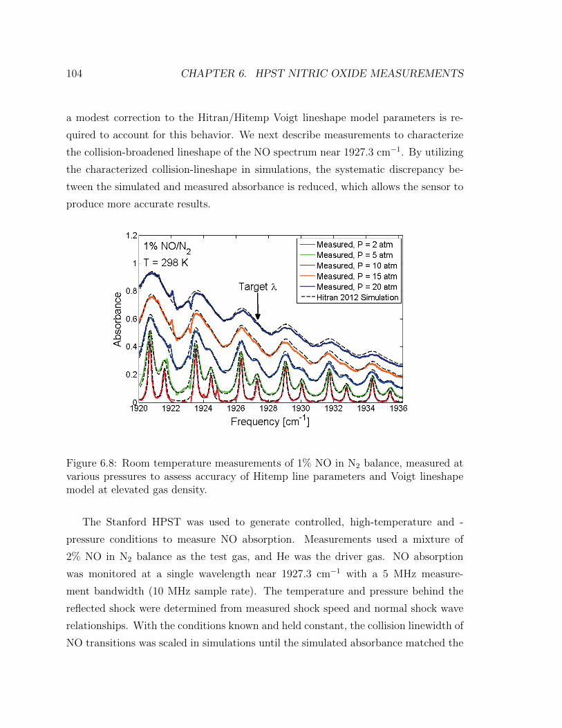
104 CHAPTER 6. HPST NITRIC OXIDE MEASUREMENTS
a modest correction to the Hitran/Hitemp Voigt lineshape model parameters is re-
quired to account for this behavior. We next describe measurements to characterize
the collision-broadened lineshape of the NO spectrum near 1927.3 cm−1. By utilizing
the characterized collision-lineshape in simulations, the systematic discrepancy be-
tween the simulated and measured absorbance is reduced, which allows the sensor to
produce more accurate results.
Figure 6.8: Room temperature measurements of 1% NO in N2 balance, measured atvarious pressures to assess accuracy of Hitemp line parameters and Voigt lineshapemodel at elevated gas density.
The Stanford HPST was used to generate controlled, high-temperature and -
pressure conditions to measure NO absorption. Measurements used a mixture of
2% NO in N2 balance as the test gas, and He was the driver gas. NO absorption
was monitored at a single wavelength near 1927.3 cm−1 with a 5 MHz measure-
ment bandwidth (10 MHz sample rate). The temperature and pressure behind the
reflected shock were determined from measured shock speed and normal shock wave
relationships. With the conditions known and held constant, the collision linewidth of
NO transitions was scaled in simulations until the simulated absorbance matched the

6.2. MEASUREMENT RESULTS 105
measured absorbance, giving a measured collision linewidth of NO with N2 as the col-
lision partner. This process was repeated in several experiments to yield the collision
linewidth, γNO−N2 , as a function of temperature. Figure 6.9 shows the results of these
measurements on a log-log scale. Also shown is the Hitemp 2012 collision linewidth
as a function of temperature and the measured parameters γ(T0) and n best-fit to the
collision linewidth coefficient function γ(T ) = γ(T0) · (T0/T )n. The best-fit linewidth
matches the Hitemp linewidth quite well, particularly at temperatures below about
1700 K where Hitemp is designed to be accurate. At higher temperatures, measure-
ments diverge from Hitemp slightly. This is entirely due to the smaller measured
temperature exponent, n, (0.655 measured versus 0.67 in Hitemp). Both measure-
ment and Hitemp agree within 0.5% that γ(T0 = 1000K) = 0.0238 cm−1. As shown
in Fig. 6.9, measurements were repeated across a broad pressure range, up to 70
atm, in order to validate that the measured lineshape had no pressure dependence, as
assumed in the model. The measured collision linewidth was then used in subsequent
experiments in order to determine the gas temperature, as discussed next.
1500 2000 2500 30000.005
0.01
0.02
Temperature [K]
me
asu
red
γN
O−
N2
(T)
[cm
−1]
P = 10−15 atmP = 20−25 atmP = 30−40 atm
P = 60−70 atmBest−FitHITEMP
n=0.655γ (T
0 = 1000 K) = 0.0238
Figure 6.9: Measured and best-fit collision linewidth for NO R(15.5) transition near1927.3 cm−1.

106 CHAPTER 6. HPST NITRIC OXIDE MEASUREMENTS
6.2.3 Thermometer Demonstration
To validate the sensor concept and demonstrate its performance, several shock tube
experiments were conducted wherein absorbance was measured near 1927.3 cm−1
across a wide range of temperatures and pressures relevant to practical facility opera-
tion. Figure 6.10 shows representative absorbance and pressure data collected in these
shock tube experiments. Here, the test gas was a non-reacting mixture of 2% NO in an
N2 balance. The first step in pressure and absorbance in Fig. 6.10, occurring near the
400 µs mark, indicates the incident shock passing over the measurement path length.
This corresponds to a nearly instantaneous rise in temperature and pressure, which
causes the absorbance to rise as well. Shortly thereafter, the reflected shock passes
back over the measurement path length, causing a further rise in temperature and
pressure and stagnating the test gas. For this particular case, the final temperature
and pressure were 1700 K and 112 atm, respectively. Note, however, that the pressure
rise between the incident shock and the reflected shock is not a step, but rather it
occurs over a finite period of time and the pressure rolls off to its steady value. This is
due to shock-bifurcation, a well-documented phenomenon in shock tubes with N2 or
air test gas (although it is not limited to only these test gases) [133, 154, 155]. Shock
bifurcation makes it difficult to resolve measurements during the first 10-50 µs after
the reflected shock passes the measurement plane. However, here we are interested
in the steady absorption signal later in the test time, and therefore these effects can
be neglected. The steady test time begins at about 550 µs on Fig. 6.10 and lasts a
total of about 350 µs.
Temperatures measured from NO absorption are shown in Fig. 6.11 against the
known temperature based on measured shock speed and normal shock relations. Mea-
sured temperature was obtained by fitting simulated absorbance with the specified
pressure and measured lineshape as fixed parameters to the measured average ab-
sorbance over the test time. The temperature corresponding to the best-fit simula-
tion is reported as the measured temperature. Two types of experiments are shown
in Fig. 6.11: 1) non-reacting mixtures of 2% NO in an N2 balance, and 2) reacting
mixtures of N2O, N2, and O2, where NO was formed in the hot, shock-heated gas.
For the reacting mixtures, temperature measurements were determined by assuming

6.2. MEASUREMENT RESULTS 107
300 400 500 600 700 800 900
0
25
50
75
100
125
Pre
ssur
e [a
tm]
Time [ s]
0.0
0.5
1.0
1.5
2.0
2.5
Steady Test Time
T = 1700 K2% NO/N2
Abs
orba
nce
Figure 6.10: Measured absorption and pressure traces in non-reacting, 2% NO in N2
balance mixture.
chemical equilibrium of the mixture, as evidenced by steady measured absorption
and pressure traces later in the test time. These two cases are distinguished in Fig.
6.11 by x-axis error bars, which are not shown for the non-reacting 2% NO mixtures
where the known temperature is based entirely on the shock counters and normal
shock relations, and is therefore accurate to within 1%. However, in the reacting
mixture, there are significant uncertainties associated with the kinetic modeling of
NO formation, and hence here the x-axis error bars shown are approximately ±3.5%.
Measured temperatures in Fig. 6.11 show good agreement with the known tem-
peratures over the range from 1150 to 2950 K and at pressures from 12 to 145 atm.
This demonstrates the accuracy of this sensor concept across a wide variety of high-
enthalpy conditions. For the non-reacting test gas mixtures, high-pressure tests below
about 2000 K display significantly smaller error bars than those at lower-pressures
and above 2000 K. This is because the uncertainty in these measurements is absorp-
tion limited, and at higher temperatures the decreased absorbance is not offset by

108 CHAPTER 6. HPST NITRIC OXIDE MEASUREMENTS
1000 1500 2000 2500 30001000
1500
2000
2500
3000
Known T [K]
Measu
red T
[K
]
P = 10−25 atmP = 30−60 atmP = 60−85 atm
P = 90−110 atmP = 120−150 atmSlope = 1
Tmeasured
=1.03 ⋅ Tknown
± 3%
Figure 6.11: Measured temperature versus known temperature across a broad rangeof temperatures and pressures. Data points with x-axis error bars were measured byobserving equilibrium formation of NO from mixtures of N2O, N2, and O2. Remainingdata points were measured in fixed-chemistry mixtures of 2% NO in N2 balance.
production of more NO, as it would be in the reacting, equilibrium NO formation
case. As temperature goes up in the fixed mixture, the NO absorption goes down,
and therefore uncertainty must grow larger. Note that for the reacting mixtures in the
region of T > 2000 K, the uncertainty in measured temperature is much smaller than
the non-reacting tests because the NO absorption grows larger rather than smaller
with increasing temperature. Also shown on Fig. 6.11 is a regression equation for
the measured versus known temperature, which gives a slope of 1.03 with an uncer-
tainty of 3%. Despite these experimental uncertainties in the non-reacting mixture,
this regression shows that the sensor concept is quite accurate over a large range of
temperatures and pressures.
Chapter 7
Summary and Future Work
In the last two decades, laser absorption spectroscopy has matured dramatically. This
includes both the development of reliable telecommunications fiber-coupled diode
lasers, the introduction of quantum cascade lasers enabling access to mid-infrared
fundamental band transitions of combustion product species, and the recent proposal
of new measurement strategies such as scanned-wavelength-modulation-spectroscopy.
Together, these developments have made laser absorption spectroscopy an increas-
ingly relevant diagnostic tool for understanding flows in advanced aeropropulsion
devices. This dissertation presented the design and results of sensor implementation
in several aeroengine test facilities, and, as summarized in the following sections, this
work has expanded the scope of our understanding of the many competing physical
processes in these complex devices.
7.1 Spatially-Resolved Measurements in an H2-Fueled,
Continuous Flow Scramjet Combustor
The design and implementation of a two-color TDLAS sensor for monitoring temper-
ature, H2O column density, and velocity was presented. The sensor was used in a
model scramjet combustor for two different geometric configurations and employed a
hybrid direct absorption-WMS strategy to account for non-uniform conditions along
109

110 CHAPTER 7. SUMMARY AND FUTURE WORK
the LOS. The measurement LOS was traversed with a system of computer-controlled
stages to sequentially shift the TDLAS LOS throughout the combustor. The sensor
targeted H2O absorption transitions at 1391.7 nm and 1469.3 nm. Measurements
were first presented for equivalence ratio Φ = 0.17 combustion in a geometry con-
sisting of a combustor and extender only. Comparisons of TDLAS measurements to
CFD simulations showed reasonable agreement in the shape over most of the product
plume. However, TDLAS detected less combustion progress overall, and in particular,
limited combustion progress between x/H = 12 and x/H = 18 near the fuel-injector
wall.
Next, measurement results were shown for a configuration with two constant area
sections added to the geometry, one upstream of the combustor and another directly
downstream of the combustor. In this configuration, the first results presented were
a H2O-seeded flow at the combustor inlet, which validated the sensor and facility
performance and showed uniform temperature and composition. Axial velocity mea-
surements for the non-combusting, H2O-seeded tests showed peak velocities through
the combustor that compare well with isentropic calculations. Temperature, col-
umn density, velocity measurements were then shown for H2-air combustion at an
equivalence ratio Φ = 0.17 and were compared to CFD simulation. Good agreement
was found between the TDLAS and CFD temperature measurements. While column
density showed reasonable agreement at x/H = 6 and x/H = 12 downstream of fuel
injection, by x/H = 18 there were significant discrepancies in both the size and shape
of the H2O product plume. However, axial velocity measurements showed excellent
agreement with CFD in the shape and magnitude of the velocity profile, particularly
at planes x/H = 6 and x/H = 15. Comparisons with CARS measurements indicate
large concentrations of combustion intermediate species in central portions of the
product plume, and that composition is consistent with near-complete combustion at
the plume edge. Finally, temperature and column density results were presented for
H2-air combustion at an equivalence ratio Φ = 0.46 along with CFD comparisons.
Agreement between TDLAS and CFD remained strong in the temperature results,
with bias towards higher temperatures predicted by CFD. TDLAS column density
results were significantly smaller than CFD predictions, suggesting less combustion

7.2. MULTISPECIES MEASUREMENTS IN A SCRAMJET 111
progress at the higher equivalence ratio. These results show that relatively simple
TDLAS measurements are a useful tool for characterizing thermophysical parameters
in harsh combustion conditions. In particular, this work has made important ad-
vances that are needed to address effects on TDLAS measurements of non-uniformity
in practical combustion facilities. The results presented comprise a useful data set for
those interested in development and evaluation of the complex flow-physics associ-
ated with scramjet propulsion. Finally, efforts made to compare these measurements
with CFD calculations provide a needed feedback for numerical modelers, who require
measurements to validate and calibrate their models.
7.2 Measurements of CO, CO2, and H2O in an
Ethylene-Fueled Scramjet
Laser absorption measurements CO, CO2 and H2O column density and CO and
H2O density-weighted temperatures were performed in the direct-connect scramjet
combustor fueled by ethylene. The model scramjet combustor had a cavity flame
holder flow path configuration fueled with ethylene-air at an overall equivalence ra-
tio of 0.15 at Mach 5 flight conditions. The sensors employed the recently-described
scanned-wavelength-modulation (scanned-WMS) spectroscopy technique using dis-
tributed feedback (DFB) quantum-cascade and DFB diode lasers for CO and H2O
measurements near 4.87 µm and 2.5 µm, respectively. These measurements provided
reliable, high-SNR signals with quantitative interpretation despite significant nonuni-
formities in temperature and composition along the sensor line-of-sight. An external-
cavity quantum-cascade laser was used for wavelength-scanned direct-absorption mea-
surements on a CO2 transition near 4.2 µm to complete the suite of multispecies mea-
surements of primary products in the ethylene-air flame. Analysis of fitting errors in
scanned-WMS integrated absorbance measurements strongly suggests that the mea-
sured fluctuations of temperature and column density are temporal variations in the
mixing and combustion efficiency (progress) at the measurement LOS and not sensor
measurement error. This interpretation is consistent with laboratory validation of the

112 CHAPTER 7. SUMMARY AND FUTURE WORK
sensors in Refs. [111, 112]. It is speculated that temporal variations in the combustor
flow field due to shear layer interaction with the cavity flame holder are the cause of
much of the observed temporal fluctuation of temperature and combustion product
column density. Measurements of temperature and column density reveal combustion
progress at each successive axial plane. However, the large observed concentration of
CO reveals incomplete combustion within the combustor. Additionally, there is virtu-
ally no temperature rise between planes, suggesting that thermal dilution of products
with the free stream air competes strongly with combustion progress, shocks, and ex-
pansions. Direct laser absorption measurements of cavity residence time during flame
extinction showed a duration of approximately 3.4 ms for column density to drop by
90% of the total dynamic range observed. This work describes the first implementa-
tion of new scanned-WMS strategies and fiber-coupled mid-IR absorption sensors to
scramjet research. Additionally, it is hoped that these measurements will provide a
useful database to compare with future computational fluid dynamics modeling of the
complex gas dynamics occurring within a hydrocarbon-fueled scramjet combustor.
7.3 Hypersonic Scramjet Combustor Measurements
The design, deployment, and use of a TDLAS sensor monitoring H2O absorption
to determine H2O column density and weighted average temperature in a model
scramjet at the HyPulse reflected shock tunnel facility was presented. This facility
provided short-duration tests of approximately 3 ms at Mach 10 flight conditions.
Scanned-WMS was used for high-SNR measurements; this work represents one of the
first implementations of this technique for absorption sensing in a practical facility.
Telecommunications lasers targeting transitions at 1391.7 nm and 1469.3 nm were
used in the sensor to deliver fiber-coupled light directly to the scramjet model within
the test cabin. Results were first shown for a non-combusting test which quantified
the presence of detonable driver gas products throughout the duration of the test
window. Two H2-air combustion cases were also presented. Both cases showed a
significant rise in column density above levels in the non-combusting case and a
temperature rise above the expected static conditions, strongly indicating the presence
7.4. HIGH-ENTHALPY AIR TEMPERATURE SENSING 113
of combustion in the model. However, the results were significantly below those
expected for complete combustion at the measurement location 27.6 cm downstream
of fuel injection. Results also showed reasonable agreement with CFD simulations
of the combustor at the same conditions, with the CFD marginally over-predicting
both extent of combustion and temperature rise compared to TDLAS results. This
work represents an important step forward in the practical implementation of TDLAS
diagnostics for detection of combustion products in hypersonic scramjet conditions.
Few other techniques offer the desirable traits of simplicity in implementation coupled
with robust diagnostic capabilities as described here, and therefore there will most
definitely be a place for these diagnostics in future hypersonic testing.
7.4 Shock Tube Measurements of Temperature in
High-T and -P Air via NO Absorption
A new sensor strategy for thermometry in high-temperature and -pressure air via
temperature-sensitive nitric oxide absorption was presented, with the purpose of char-
acterizing test facility conditions. The sensor utilizes the monotonic increase in equi-
librium NO mole fraction with temperature, and the independence of mole fraction
with pressure. As a result, strong mid-infrared absorption of NO near 5.2 µm is highly
temperature sensitive and can be utilized to characterize the temperature of air across
a wide range of pressures and temperatures. The NO R(15.5) transition near 1927.3
cm−1 was selected for its avoidance of nearby H2O interference and accessibility with
a high-power external-cavity quantum-cascade laser source. A demonstration of the
sensor concept was performed. First, room temperature measurements of the NO
spectrum from 1920 cm−1 to 1936 cm−1 verified that only small corrections to the
Hitemp database spectral parameters are needed to account for non-Lorentzian col-
lision effects at gas densities above 10 Amagat. These corrections were incorporated
into the Voigt lineshape model by characterizing the collision linewidth as a function
of temperature in shock-tube experiments at pressures ranging from 10 to 70 atm.
Finally, the sensor performance was demonstrated via measurements of temperature

114 CHAPTER 7. SUMMARY AND FUTURE WORK
over the range of 1100 to 2950 K and 12 to 145 atm, in both non-reacting NO seeded
experiments, and reacting experiments where NO was formed in the hot, shock-heated
gas. The sensor provided accurate measurements of temperature over this entire do-
main, and is a promising method for improving high-enthalpy facility operation and
characterization.
7.5 Future Work
Practical, air-breathing hypersonic propulsion devices remain elusive despite decades
of research. While researchers have made important strides in understanding of these
systems, barriers still exist in our understanding. Turbulent mixing, combustion and
heat transfer in scramjet combustors is exceedingly complicated and their theory is
not yet on firm ground. Other problems such as shock-boundary layer interaction
continue to plague both practical facilities as well as well as numerical modelers. So,
there is a continued role to be played for robust diagnostic measurements, capable
of illuminating the physical processes that drive these phenomena. Researchers have
many diagnostic methods to choose from, but over the decades, laser absorption spec-
troscopy has earned its place as a tool of choice because of ease of implementation and
powerful measurement capabilities. Those capabilities have grown dramatically in the
last ten years, with each generation of sensor substantially improving measurement
fidelity over previous iterations. The work presented here represents one small part
of those improvements, but there are many more opportunities to improve further.
Here, we outline some potential directions for future work.
7.5.1 High-Bandwidth Measurements in a Hypersonic Test
Facility
The Mach 10 scramjet combustor measurements presented in Chapter 5 were the first
WMS measurements of their kind, and as such they are an important step in imple-
menting advanced optical diagnostics within an impulse facility capable of creating
these hypersonic conditions. Those measurements utilized scanned-WMS to provide
7.5. FUTURE WORK 115
measurements with a bandwidth of 1 kHz, or six measurement points over a 3 ms
test time. While these measurements were sufficient to identify ignition onset as well
as other basic trends such as increasing combustion progress over the course of a sin-
gle test, the relatively low bandwidth relative to the test time significantly hindered
the depth of interpretation allowed by the data. Future measurements with higher
bandwidth would offer greater insight into combustion progress at high Mach num-
bers, and a better understanding of unsteady combustion dynamics within hypersonic
scramjet combustors.
Measurements from Chapter 5 took place during winter at the HyPulse facility
in Ronkonkoma, NY. At the time it was found that changes in the ambient facility
temperature were large enough that the laser temperature controller could not hold
the lasers at a constant wavelength. Fixed-wavelength experiments were therefore
impractical, and only wavelength-scanned-WMS offered both insensitivity to laser
set-point drift as well as excellent signal-to-noise ratio needed in a noisy experimental
facility. This technique was only in its infancy at the time, therefore the scan-rate
was restricted to 1 kHz based on experience with calibration-free WMS experiments.
However, there is no reason that scanned-WMS measurements can not be applied to
measurements with a scan rate far in excess of 1 kHz (although, the scan frequency
should still be smaller than the modulation frequency). The only caveat on this
statement is that the model presented in Chapter 2 for the laser wavelength and
output intensity (Eqs. (2.12) to (2.17)) assumes that terms higher than the second
harmonic, and cross-product terms can be neglected. This assumption may not be
satisfied at very high scan-rates, and therefore care should be taken to either use
an appropriate model for laser dynamics, or simply measure the baseline intensity
directly. However, if these conditions are satisfied, high-bandwidth scanned-WMS
measurements in a hypersonic scramjet combustor should be possible, and would
provide a new and valuable piece of information to the community of researchers
interested in scramjet engines.

116 CHAPTER 7. SUMMARY AND FUTURE WORK
7.5.2 Facility Characterization via Nitric Oxide Absorption
Sensor
The motivation, design, and initial demonstration of a temperature sensor for high-
enthalpy air by monitoring nitric oxide absorption was presented in Chapter 6. An
important next step would be to implement this sensor strategy to characterize the
inlet flow in a practical test facility. In addition to this test providing a true vali-
dation of the sensor concept, it would also produce valuable information needed by
both facility operators who want to know if their hardware is operating on target,
as well as computational modelers who are trying to compare simulations to exper-
imental data collected in that particular facility. To accomplish this, considerable
effort must be placed in engineering the optical system to deliver 5.2 µm light to
the test article and detect transmitted signals, while maintaining robust alignment
in the face of inevitable facility noise due to mechanical vibration and beam steer-
ing, etc. Hollow-core fiber like that which was used to deliver mid-infrared infrared
light to the University of Virginia scramjet combustor in Chapter 4 could be used for
this application as well [113, 156]. Adding multiple wavelengths to the sensor would
complicate the optical engineering slightly, but has many potential benefits. A non-
absorbing reference beam would reduce measurement sensitivity to non-absorption
losses due to vibration, scatting, beam steering, or window birefringence [146]. A sec-
ond wavelength targeting an NO transition with a different temperature sensitivity
would allow the sensor to provide two independent temperature measurements, one
from two-color direct absorption and the other from assuming NO is in equilibrium
and solving for temperature using a single transition (as in the work presented in
this dissertation). This approach would also test the equilibrium assumption, since
a two-line sensor can also solve for the NO concentration directly and compare that
value to the NO expected to be present in the equilibrium mixture.
7.5.3 TDLAS for Flight Testing
While the work in this dissertation has focused on absorption diagnostics for ground
test facilities, it also bears mentioning that TDLAS sensors hold great promise flight

7.5. FUTURE WORK 117
testing. Already, TDLAS sensors have been used in two flight-test experiments by
NASA, the Air Force Research Laboratory (AFRL), and Australia’s Defense Science
and Technology Organization (DSTO) under the banner of HIFiRE [157–159]. These
tests showed that laser absorption sensors can be designed with a small enough hard-
ware footprint for flight testing, all while maintaining good optical alignment and
sufficient insensitivity to harsh flight test conditions. However, these tests only rep-
resent a small piece of what TDLAS sensors may be used for the future. For exper-
imental flight testing sensors, WMS methods including both calibration-free WMS
and scanned-WMS offer the potential to improve the quality of measurements. Even-
tually, new laser technology may also enable the monitoring of species beyond O2
and H2O as demonstrated in the HIFiRE experiments, which would allow a better
understanding of hydrocarbon combustion in scramjets within the most practical con-
ditions imaginable. Additionally, there is also an opportunity to develop absorption
diagnostics for in-flight, real-time monitoring combustion. Previously Rieker, et al.
used a TDLAS sensor to detect unstart in a scramjet engine [26]. It may be possible
to install a similar sensor into a flight system to detect unstart, to provide feedback
for active control, or to monitor engine emissions.

Appendix A
A Numerical Solution for
Peak-WMS Measurements
Measurements of the peak WMS-2f /1f signal are related to the temperature and
species column density through a nonlinear set of equations that in general have no
explicit solution. Therefore, one must devise a numerical approach for converting
these WMS signals into quantitative thermodynamic measurements. One approach
that has been used successfully in the past is to simulate the WMS signal over a range
of gas temperatures, pressures, and column densities using the theoretical framework
described in Section 2.3 at the characterized laser settings (modulation depth and laser
dynamics). The measured signals can then be compared to the array of simulated
values to make quantitative measurements. While this technique is effective, it does
not scale favorably when additional parameters are accounted for. For instance, when
nonuniform conditions along the laser line-of-sight (LOS) are considered, the empirical
collision linewidth of the absorption feature must be included in calculations to make
quantitatively accurate measurements. In these situations, it is worthwhile to make
use of numerical solution techniques that do not require brute-force simulations over
a large domain of potential temperature, pressure, composition, and collisional width
conditions. A multidimensional Newton-Raphson algorithm offers a simple method
of iteratively simulating WMS signals at guess values of temperature and column
density with fixed collisional width (to account for LOS nonuniformity) and fixed
118

A.1. THE NEWTON-RAPHSON METHOD 119
modulation depth and laser characteristics.
Simulating WMS signals by brute-force over a range of temperature, pressure, and
mole fraction conditions takes several hours of computation. Moreover, adding an ad-
ditional degree of freedom such as collisional width extends the computation time to
days. In contrast, a properly implemented Newton-Raphson technique gives numer-
ically identical results in as few as 7 seconds based on the Matlab implementation
used in this study.
A.1 The Newton-Raphson Method
The Newton-Raphson method is a numerical root-finding technique that is described
here in a single dimension to offer a basic explanation of the solution method. We
seek the solution to the function y = f (x), by finding the root of the equation
y − f (x) = 0. We begin by supplying the algorithm with an initial guess value for
the solution, x0, and then evaluate the function and its derivative at x0. The guess
value x0 is updated by tracing the derivative f ′(x0) from the point f(x0) back to the
line y = 0. This process is given by the Eq. (A.1) below:
x1 = x0 −f(x0)
f ′(x0)(A.1)
In most cases, the updated guess value will be closer to the true root of the function.
The accuracy of the solution can be improved by using the new guess value to make
an additional updates to the solution iteratively. Generally, the updated guess value
will always take the form:
xj+1 = xj −f(xj)
f ′(xj)(A.2)
The algorithm is stopped by the user when the function value at the guess is within
a specified tolerance of zero. This iterative process is shown graphically in Fig. A.1
for the first five updates of the root guess value of a polynomial function. For this
particular function, after five iterations the guess value is very close to the actual
root.

120APPENDIX A. A NUMERICAL SOLUTION FOR PEAK-WMSMEASUREMENTS
0
X
f(X
)
0
X
f(X
)
f(x0)
x0
x1
f(x1)
x2
f(x2)
x3
f(x3)
f(x4)
x4
x5
Figure A.1: Graphical representation of Newton’s method for a one-dimensional func-tion.
A.2 Newton’s Method Applied to WMS
With WMS, as with any two-line sensor for temperature and composition, one line
is used to solve for column density and the ratio of both lines is used to solve for
temperature. The solution of these two equations are coupled, however, which ne-
cessitates a simultaneous solution and therefore multivariate approach. We begin by
assuming that the user has supplied measured WMS-2f /1f peak signals from each of
a pair of lines, to be denoted S12f/1f and S2
2f/1f . From Section 2.3, the WMS signals
can be written as functions of temperature T , pressure P , composition N (determined
by the column density of constituent species), and laser characteristics such as the
center-wavelength of the laser ν, modulation depth a1,m, and the amplitudes of the
laser harmonics i1,m and i2,m. Additionally, the WMS signal may depend on other
parameters such as the collisional width of the absorption lineshape (∆νc) in cases
where it is fixed in order to account for nonuniform conditions along the measurement
line-of-sight. Here we consider only the general function of WMS signals of the form

A.2. NEWTON’S METHOD APPLIED TO WMS 121
shown in Eq. (A.3) for a laser targeting transition k.
Sk2f/1f = f(T,N, P,∆νkc , ν
k, ak, ik1,m, ik2,m
)(A.3)
Although the laser characteristics are considered constants in Eq. (A.3), it is impor-
tant to recognize that these parameters will change whenever any of the laser settings
are changed, and therefore they are shown as variables above. The exact functional
form of Eq. (A.3) is not explicitly stated because it is overly lengthy and complicated.
Generally, the best practice when simulating WMS signals is to break the calculation
into its constituent pieces as described in Sections 2.2 and 2.3; first compute the ab-
sorbance over the entire wavelength range, and then use this absorbance as an input
to simulate the WMS lineshape.
For this application, Newton’s method seeks the solution to the following equation: R =S22f/1f
S12f/1f
S12f/1f
=
[g (T,N, P,∆ν1c ,∆ν
2c )
f (T,N, P,∆ν1c , )
](A.4)
This equation can be approximated using a Taylor series expansion about T +δT and
N + δN , including only the first-order terms, as shown in Eq. (A.5):[g (T + δT,N + δN)
f (T + δT,N + δN)
]≈
[g (T,N)
f (T,N)
]+
[∂g∂T
∂g∂N
∂f∂T
∂f∂N
][δT
δN
](A.5)
The goal of the multivariate Newton’s method in the case of WMS is to use Eq. (A.5)
to solve for the δT and δN needed in order to achieve equality. In other words, each
iteration seeks to update the guess values of temperature and column density for the
solution to Eq. (A.4) by solving Eq. (A.5) for the magnitude of the change in the
guess values.
In practice, the algorithm begins by computing the simulated peak WMS-2f /1f
values at the specified temperature and column density values supplied by the user’s
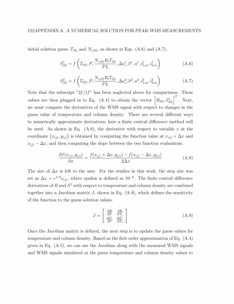
122APPENDIX A. A NUMERICAL SOLUTION FOR PEAK-WMSMEASUREMENTS
initial solution guess, T(0) and Ni,(0), as shown in Eqs. (A.6) and (A.7).
S1(0) = f
(T(0), P,
Ni,(0)RiT(0)PL
,∆ν1c , ν1, a1, ij1,m, i
12,m
)(A.6)
S2(0) = f
(T(0), P,
Ni,(0)RiT(0)PL
,∆ν2c , ν2, a2, i21,m, i
22,m
)(A.7)
Note that the subscript “2f /1f ” has been neglected above for compactness. These
values are then plugged in to Eq. (A.4) to obtain the vector[R(0), S
1(0)
]T. Next,
we must compute the derivatives of the WMS signal with respect to changes in the
guess value of temperature and column density. There are several different ways
to numerically approximate derivatives; here a finite central difference method will
be used. As shown in Eq. (A.8), the derivative with respect to variable x at the
coordinate(x(j), y(j)
)is obtained by computing the function value at x(j) + ∆x and
x(j) − ∆x, and then computing the slope between the two function evaluations.
∂f(x(j), y(j))
∂x=f(x(j) + ∆x, y(j)) − f(x(j) − ∆x, y(j))
2∆x(A.8)
The size of ∆x is left to the user. For the studies in this work, the step size was
set as ∆x = ε1/3x(j), where epsilon is defined as 10−6. The finite central difference
derivatives of R and S1 with respect to temperature and column density are combined
together into a Jacobian matrix J , shown in Eq. (A.9), which defines the sensitivity
of the function to the guess solution values.
J =
[∂R∂T
∂R∂Ni
∂S1
∂T∂S1
∂Ni
](A.9)
Once the Jacobian matrix is defined, the next step is to update the guess values for
temperature and column density. Based on the first-order approximation of Eq. (A.4)
given in Eq. (A.5), we can use the Jacobian along with the measured WMS signals
and WMS signals simulated at the guess temperature and column density values to

A.2. NEWTON’S METHOD APPLIED TO WMS 123
estimate how much our guess values should change.[δT
δNi
]= J−1
([R(j)
S1(j)
]−
[RmeasuredS1
measured
])(A.10)
Here δT and δNi are the estimated changes in the guess value needed, as shown in
Eq. (A.11). [T(j+1)
Ni,(j+1)
]=
[T(j)
Ni,(j)
]+
[δT
δNi
](A.11)
At this point, the algorithm has updated the guess values for temperature and column
density, and the user may either stop the algorithm and consider T(j+1) and Ni,(j+1)
the solution, or the user may use these updated guess values for continued iteration.
Whether to continue iterating or not depends on convergence of the change in guess
values to within machine accuracy, and the convergence of the functions f and g to
within machine accuracy. Once either set has converged, the other will no longer
change.
Usually, implementing the preceding algorithm will give sufficiently accurate so-
lutions after only a few iterations. However, if the initial guesses of temperature
and column density is not close enough to the solution value, Newton’s method may
sometimes erroneously propose large steps that may cause the method to converge on
an erroneous solution or diverge altogether. Therefore, to help ensure convergence,
it is sometimes advantageous to not take the full step in δT and δN . If a case is
discovered where Newton’s method will not converge, an algorithm is presented in
Ref. [160] to optimally backtrack along the full Newton’s method step.

Bibliography
[1] M. S. Richman, J. A. Kenyon, and R. M. Sega, “High speed and hypersonic
science and technology,” in “41st AIAA/ASME/SAE/ASEE Joint Propulsion
Conference and Exhibit,” (AIAA, 2005). Tucson, AZ.
[2] A. Ferri, “Review of SCRAMJET propulsion technology,” Journal of Aircraft
5, 3–10 (1968).
[3] M. M. Roy, “Moteurs thermiques,” Comptes rendus de l’Academie des Sciences
222, 31 – 32 (1946).
[4] E. T. Curran, W. H. Heiser, and D. T. Pratt, “Fluid phenomena in scramjet
combustion systems,” Annual Review of Fluid Mechanics 28, 323–360 (1996).
[5] W. H. Sargent and R. A. Gross, “Detonation wave hypersonic ramjet,” ARS
Journal 30, 543–549 (1960).
[6] R. A. Gross and W. Chinitz, “A study of supersonic combustion,” Journal of
the Aerospace Sciences 27, 517–524 (1960).
[7] J. P. Sislian, “Detonation-wave ramjets,” in “Scramjet Propulsion,” , vol. 189
of Progress in Astronautics and Aeronautics, E. T. Curran and S. N. B. Murthy,
eds. (American Institute of Aeronautics and Astronautics, Reston, VA, 2001).
[8] A. Ferri, P. A. Libby, and V. Zakkay, “Theoretical and experimental investiga-
tions of supersonic combustion,” in “Proceedings of the International Council
of the Aeronautical Sciences, Third Congress,” (Spartan, 1962). Stockholm,
Sweeden.
124

BIBLIOGRAPHY 125
[9] A. Ferri, “Mixing-controlled supersonic combustion,” Annual Review of Fluid
Mechanics 5, 301–338 (1973).
[10] E. T. Curran, “Scramjet engines: The first forty years,” Journal of Propulsion
and Power 17, 1138–1148 (2001).
[11] J. L. Wagner, A. Valdivia, K. B. Yuceil, N. T. Clemens, and D. S. Dolling, “An
experimental investigation of supersonic inlet unstart,” in “37th AIAA Fluid
Dynamics Conference and Exhibit,” (AIAA, 2007). Miami, FL.
[12] Q. Wang, K. Duraisamy, J. J. Alonso, and G. Iaccarino, “Risk assessment of
scramjet unstart using adjoint-based sampling methods,” AIAA Journal 50,
581 – 592 (2012).
[13] J. M. Seiner, S. M. Dash, and D. C. Kenzakowski, “Historical survey on en-
hanced mixing in scramjet engines,” Journal of Propulsion and Power 17, 1273–
1286 (2001).
[14] D. B. Le, C. P. Goyne, R. H. Krauss, and J. C. McDaniel, “Experimental
study of a dual-mode scramjet isolator,” Journal of Propulsion and Power 24,
1050–1057 (2008).
[15] G. B. Northam and G. Y. Anderson, “Survey of supersonic combustion ramjet
research at Langley,” in “24th Aerospace Sciences Meeting,” (AIAA, 1986).
Reno, NV.
[16] J. M. Tishkoff, J. P. Drummond, T. Edwards, and A. S. Nejad, “Future di-
rections of supersonic combustion research – Air Force/NASA workshop on
supersonic combustion,” in “35th AIAA Aerospace Sciences Meeting,” (AIAA,
1997). Reno, NV.
[17] W. E. White, J. P. Drummond, and A. Kumar, “Evolution and application of
CFD techniques for scramjet engine analysis,” Journal of Propulsion and Power
3, 423 – 439 (1987).
126 BIBLIOGRAPHY
[18] N. C. Bissinger, “CFD support for scramjet design and testing,” in “9th AIAA
International Space Planes and Hypersonic Systems and Technologies Confer-
ence,” (AIAA, 1999). Norfolk, VA.
[19] F. Ladeinde, “A critical review of scramjet combustion simulation,” in “47th
AIAA Aerospace Sciences Meeting,” (AIAA, 2009). Orlando, FL.
[20] R. A. Baurle, “Modeling of high speed reacting flows: Established practices and
future challenges,” in “42nd AIAA Aerospace Sciences Meeting and Exhibit,”
(AIAA, 2004). Reno, NV.
[21] M. Oevermann, “Numerical investigation of turbulent hydrogen combustion in
a scramjet using flamelet modeling,” Aerospace Science and Technology 4, 463
– 480 (2000).
[22] R. D. Rockwell, C. P. Goyne, B. E. Rice, B. J. Tatman, C. Smith, T. Kouchi,
J. C. McDaniel, J. A. Fulton, and J. R. Edwards, “Close-collaborative experi-
mental and computational study of a dual-mode scramjet combustor,” in “50th
AIAA Aerospace Sciences Meeting,” (AIAA, 2012). Nashville, TN.
[23] A. C. Eckbreth, Laser Diagnostics for Combustion Temperature and Species
(Overseas Publishers Association, Amsterdam B.V., The Netherlands, 1996).
[24] W. G. Spangenberg and W. R. Rowland, “Optical study of boundary-layer
transition processes in a supersonic air stream,” Physics of Fluids 3, 667–684
(1960).
[25] I. A. Schultz, C. S. Goldenstein, R. M. Spearrin, J. B. Jeffries, R. K. Han-
son, R. D. Rockwell, and C. P. Goyne, “Multispecies mid-infrared absorption
measurements in a hydrocarbon-fueled scramjet combustor,” (2014). Journal of
Propulsion and Power (in press).
[26] G. B. Rieker, J. B. Jeffries, and R. K. Hanson, “Diode laser-based detection of
combustor instabilities with application to a scramjet engine,” Proceedings of
the Combustion Institute 32, 831–838 (2009).

BIBLIOGRAPHY 127
[27] R. L. McKenzie, “Progress in laser spectroscopic techniques for aerodynamic
measurement: An overview,” AIAA Journal 31, 465 – 477 (1993).
[28] R. R. Boyce, N. R. Mudford, and J. R. McGuire, “OH-PLIF visualisation of
radical farming supersonic combustion flows,” Shock Waves 22, 9–21 (2012).
[29] J. M. Donbar, M. R. Gruber, T. A. Jackson, C. D. Carter, and T. Mathur, “OH
planar laser-induced fluoroescence imaging in a hydrocarbon-fueled scramjet
combustor,” Proceedings of the Combustion Institute 28, 679–687 (2000).
[30] B. K. McMillin, J. M. Seitzman, and R. K. Hanson, “Comparison of NO and OH
planar fluorescence temeprature measurements in scramjet model flowfields,”
AIAA Journal 32, 1945 – 1952 (1994).
[31] A. C. Eckbreth, T. J. Anderson, and G. M. Dobbs, “Multi-color CARS for
hydrogen-fueled scramjet applications,” Applied Physics B 45, 215–223 (1988).
[32] K. A. Vereschagin, V. V. Smirnov, O. M. Stelmakh, V. I. Fabelinsky, V. A.
Sabelnikov, V. V. Ivanov, W. Clauss, and M. Oschwald, “Temperature measure-
ments by coherent anti-stokes raman spectroscopy in hydrogen-fuelled scramjet
combustor,” Aerospace Science and Technology 5, 347–355 (2001).
[33] A. D. Cutler, G. Magnotti, L. Cantu, E. Gallo, R. D. Rockwell, and C. P.
Goyne, “Dual-pump coherent anti-stokes raman spectroscopy measurements in
a dual-mode scramjet,” Journal of Propulsion and Power (2014). (in press).
[34] C. T. Smith and C. P. Goyne, “Three-component velocimetry in a scramjet
combustor,” in “44th AIAA/ASME/SAE/ASEE Joint Propulsion Conference
and Exhibit,” (AIAA, 2008). Hartford, CT.
[35] J. Xu, J. Ma, J. Mo, and K. Zhang, “PIV experimental and numerical inves-
tigation of cold flowfield of scramjet combustor with inlet/isolator,” in “17th
AIAA International Space Planes and Hypersonic Systems and Technologies
Conference,” (AIAA, 2011). San Francisco, CA.

128 BIBLIOGRAPHY
[36] R. K. Hanson, “Applications of quantitative laser sensors to kinetics, propulsion
and practical energy systems,” Proceedings of the Combustion Institute 33, 1
– 40 (2011).
[37] L. C. Philippe and R. K. Hanson, “Laser-absorption mass flux sensor for high-
speed airflows,” Optics Letters 16, 2002–2004 (1991).
[38] R. K. Hanson, “Laser-based diagnostics for hypersonic flows,” in “New Trends
in Instrumentation for Hypersonic Research,” , vol. 224 of NATO ASI Series,
A. Boutier, ed. (American Institute of Aeronautics and Astronautics, Chatillon,
France, 1993).
[39] M. G. Allen, “Diode laser absorption sensors for gas-dynamic and combustion
flows,” Measurement Science and Technology 9, 545–562 (1998).
[40] R. M. Mihalcea, M. E. Webber, D. S. Baer, R. K. Hanson, G. S. Feller, and
W. B. Chapman, “Diode-laser absorption measurements of CO2, H2O, N2O,
and NH2 near 2.0 µm,” Applied Physics B 67, 283 – 288 (1998).
[41] A. Farooq, J. B. Jeffries, and R. K. Hanson, “CO2 concentration and temper-
ature sensor for combustion gases using diode-laser absorption near 2.7 µm,”
Applied Physics B 90, 619–628 (2008).
[42] S. T. Sanders, J. A. Baldwin, T. P. Jenkins, D. S. Baer, and R. K. Hanson,
“Diode-laser sensor for monitoring multiple combustion parameters in pulse det-
onation engines,” Proceedings of the Combustion Institute 28, 587–594 (2000).
[43] J. Wang, M. Maiorov, D. S. Baer, D. Z. Garbuzov, J. C. Connolly, and R. K.
Hanson, “In situ combustion measurements of CO with diode-laser absorption
near 2.3 µm,” Applied Optics 39, 5579 – 5589 (2000).
[44] R. K. Hanson, D. S. Baer, B. K. Mcmillin, and M. P. Arroyo, “Flow and parti-
cle diagnostics. multi-parameter and multi-point measurements,” Berichte der
Bunsengesellschaft fur physikalische Chemie 97, 1548 – 1554 (1993).

BIBLIOGRAPHY 129
[45] M. P. Arroyo, T. P. Birbeck, D. S. Baer, and R. K. Hanson, “Dual diode-
laser fiber-optic diagnostic for water-vapor measurements,” Optics Letters 19,
1091–1093 (1994).
[46] L. C. Philippe and R. K. Hanson, “Sensitive diode laser absorption technique
for aerodynamic measurements,” in “30th Aerospace Sciences Meeting and Ex-
hibit,” (AIAA, 1992). Reno, NV.
[47] A. C. Stanton, D. S. Bomse, and J. A. Silver, “A nonintrusive diagnostic for
water vapor in high temperature flow fields,” Tech. Rep. R90-01, Southwest
Sciences, Inc., Santa Fe, NM (1991).
[48] M. P. Arroyo and R. K. Hanson, “Tunable diode laser absorption technique
for detection of water vapor in aerodynamic flows,” in “30th AIAA Aerospace
Sciences Meeting and Exhibit,” (AIAA, 1992). Reno, NV.
[49] M. P. Arroyo and R. K. Hanson, “Absorption measurements of water-vapor con-
centration, temperature, and line-shape parameters using a tunable InGaAsP
diode laser,” Applied Optics 32, 6104–6116 (1993).
[50] B. L. Upschulte, M. F. Miller, M. G. Allen, K. Jackson, M. Gruber, and
T. Mathur, “Continuous water vapor mass flux and temperature measurements
in a model scramjet combustor using a diode laser sensor,” in “37th AIAA
Aerospace Sciences Meeting,” (AIAA, 1999). Reno, NV.
[51] C. Y. Tsai, “A two-line absorption instrument for scramjet temperature and
water vapor concentration measurement in HYPULSE,” Tech. Rep. NASA CR-
1998-207664, NASA, National Aeronautics and Space Administration, Washin-
ton, DC 20546 (1998).
[52] D. S. Baer, R. K. Hanson, M. E. Newfield, and N. K. J. M. Gopaul, “Multi-
plexed diode-laser sensor system for simultaneous H2O, O2, and temperature
measurements,” Optics Letters 19, 1900–1902 (1994).

130 BIBLIOGRAPHY
[53] E. B. Bryner, G. S. Diskin, C. P. Goyne, J. C. McDaniel, R. H. Krauss, and
T. A. Slate, “Water vapor concentration measurement in high enthalpy flows us-
ing infrared absorption,” in “39th AIAA/ASME/SAE/ASEE Joint Propulsion
Conference and Exhibit,” (AIAA, 2003). Huntsville, AL.
[54] A. J. Houle, K. Nakakita, W. N. Heltsley, J. B. Jeffries, and R. K. Hanson,
“Diode laser absorption measurements of supersonic flow in an expansion tube,”
in “42nd AIAA/ASME/SAE/ASEE Joint Propulsion Conference and Exhibit,”
(AIAA, 2006). Sacramento, CA.
[55] S. Chen, J. A. Silver, D. S. Bomse, C. C. Rassmussen, and J. F. Driscoll,
“Combustion species sensor for scramjet flight instrumentation,” in “41st
AIAA/ASME/SAE/ASEE Joint Propulsion Conference and Exhibit,” (AIAA,
2005). Tucson, AZ.
[56] M. Gruber, C. Carter, M. Ryan, G. B. Rieker, J. B. Jeffries, R. K. Han-
son, J. Liu, and T. Mathur, “Laser-based measurements of OH, temperature,
and water vapor concentration in a hydrocarbon-fueled scramjet,” in “44th
AIAA/ASME/SAE/ASEE Joint Propulsion Conference and Exhibit,” (AIAA,
2008). Hartford, CT.
[57] L. C. Philippe and R. K. Hanson, “Laser diode wavelength-modulation spec-
troscopy for simultaneous measurement of temperature, pressure, and velocity
in shock-heated oxygen flows,” Applied Optics 32, 6090–6103 (1993).
[58] M. S. Brown, D. L. Barone, T. F. Barhorst, D. Eklund, and M. Gruber,
“TDLAS-based measurements of temperature, pressure, and velocity in the iso-
lator of an axisymmetric scramjet,” in “46th AIAA/ASME/SAE/ASEE Joint
Propulsion Conference and Exhibit,” (AIAA, 2010). Nashville, TN.
[59] F. Li, X. Yu, H. Gu, Z. Li, L. Chen, and X. Chang, “Measurement of temper-
ature, velocity and water vapor concentration in a scramjet combustor based
on near-infrared diode laser absorption,” in “17th AIAA International Space

BIBLIOGRAPHY 131
Planes and Hypersonic Systems and Technologies Conference,” (AIAA, 2011).
San Francisco, CA.
[60] D. S. Baer, H. A. Chang, and R. K. Hanson, “Semiconductor laser absorption
diagnostics of atomic oxygen in an atmospheric-pressure plasma,” Journal of
Quantitative Spectroscopy and Radiative Transfer 50, 621–633 (1993).
[61] J. T. C. Liu, G. B. Rieker, J. B. Jeffries, M. R. Gruber, C. D. Carter, T. Mathur,
and R. K. Hanson, “Near-infrared diode laser absorption diagnostic for temper-
ature and water vapor in a scramjet combustor,” Applied Optics 44, 6701–6711
(2005).
[62] A. D. Griffiths and A. F. P. Houwing, “Measurements of temperature and water
vapour concentration in a scramjet combustor,” in “15th Australasian Fluid
Mechanics Conference,” (2004). Sydney, Australia.
[63] L. S. Chang, C. L. Strand, J. B. Jeffries, R. K. Hanson, G. S. Diskin, R. L.
Gaffney, and D. P. Capriotti, “Supersonic mass-flux measurements via tunable
diode laser absorption and nonuniform flow modeling,” AIAA Journal 49, 2783–
2791 (2011).
[64] J. Humlıcek, “Optimized computation of the Voigt and complex probability
functions,” Journal of Quantitative Spectroscopy and Radiative Transfer 27,
437 – 444 (1982).
[65] C. S. Goldenstein, I. A. Schultz, J. B. Jeffries, and R. K. Hanson, “Two-color
absorption spectroscopy strategy for measuring the column density and path
average temperature of the absorbing species in nonuniform gases,” Applied
Optics 52, 7950–7962 (2013).
[66] D. S. Bomse, A. C. Stanton, and J. A. Silver, “Frequency modulation and
wavelength modulation spectroscopies: comparison of experimental methods
using a lead-salt diode laser,” Applied Optics 31, 718–731 (1992).

132 BIBLIOGRAPHY
[67] J. Wolfrum, “Lasers in combustion: From basic theory to practical devices,”
Proceedings of the Combustion Institute 27, 1 – 41 (1998).
[68] J. A. Silver, “Frequency-modulation spectroscopy for trace species detection:
Theory and comparison among experimental methods,” Applied Optics 31,
707–717 (1992).
[69] J. Reid and D. Labrie, “Second-harmonic detection with tunable diode lasers–
comparison of experiment and theory,” Applied Physics B 26, 203–210 (1981).
[70] G. B. Rieker, J. B. Jeffries, and R. K. Hanson, “Calibration-free wavelength-
modulation spectroscopy for measurements of gas temperature and concentra-
tion in harsh environments,” Applied Optics 48, 5546–5560 (2009).
[71] H. Li, G. B. Rieker, X. Liu, J. B. Jeffries, and R. K. Hanson, “Extension of
wavelength-modulation spectroscopy to large modulation depth for diode laser
absorption measurements in high-pressure gases,” Applied Optics 45, 1052 –
1061 (2006).
[72] X. Liu, J. B. Jeffries, and R. K. Hanson, “Measurements of spectral parameters
of water-vapour transitions near 1388 and 1345 nm for accurate simulation of
high-pressure absorption spectra,” Measurement Science and Technology 18,
1185 (2007).
[73] X. Chao, J. B. Jeffries, and R. K. Hanson, “Real-time, in situ, continuous
monitoring of CO in a pulverized-coal-fired power plant with a 2.3 µm laser
absorption sensor,” Applied Physics B 110, 359–365 (2013).
[74] K. Sun, R. Sur, X. Chao, J. B. Jeffries, R. K. Hanson, R. J. Pummill, and K. J.
Whitty, “TDL absorption sensors for gas temperature and concentrations in
a high-pressure entrained-flow coal gassifier,” Proceedings of the Combustion
Institute 34, 3593–3601 (2012).
[75] H. Li, S. D. Wehe, and K. R. McManus, “Real-time equivalence ratio mea-
surements in gas turbine combustors with a near-infrared diode laser sensor,”
Proceedings of the Combustion Institute 33, 717 – 724 (2011).

BIBLIOGRAPHY 133
[76] R. M. Spearrin, C. S. Goldenstein, J. B. Jeffries, and R. K. Hanson, “Fiber-
coupled 2.7 µm laser absorption sensor for CO2 in harsh combustion environ-
ments,” Measurement Science and Technology 24, 055107 (2013).
[77] J. M. Supplee, E. A. Whittaker, and W. Lenth, “Theoretical description of fre-
quency modulation and wavelength modulation spectroscopy,” Applied Optics
33, 6294–6302 (1994).
[78] P. Kluczynski and O. Axner, “Theoretical description based on Fourier analysis
of wavelength-modulation spectrometry in terms of analytical and background
signals,” Applied Optics 38, 5803–5815 (1999).
[79] M. Lackner, “Tunable diode laser absorption spectroscopy (TDLAS) in the
process industries - a review,” Reviews in Chemical Engineering 23, 65–147
(2007).
[80] C. L. Strand and R. K. Hanson, “Thermometry and velocimetry in supersonic
flows via scanned wavelength-modulation absorption spectroscopy,” in “47th
Joint Propulsion Conference,” (AIAA, 2011). San Diego, CA.
[81] D. T. Cassidy and J. Reid, “Atmospheric pressure monitoring of trace gases
using tunable diode lasers,” Applied Optics 21, 1185–1190 (1982).
[82] C. S. Goldenstein, C. L. Strand, I. A. Schultz, K. Sun, J. B. Jeffries, and
R. K. Hanson, “Fitting of calibration-free scanned-wavelength-modulation spec-
troscopy spectra for determination of gas properties and absorption linesahpes,”
Applied Optics 53, 356–367 (2014).
[83] G. B. Rieker, J. B. Jeffries, and R. K. Hanson, “Measurements of high-pressure
CO2 absorption near 2.0 µm and implications on tunable diode laser sensor
design,” Applied Physics B pp. 51–63 (2008).
[84] K. Sun, X. Chao, R. Sur, C. S. Goldenstein, J. B. Jeffries, and R. K. Hanson,
“Analysis of calibration-free wavelength-scanned wavelength modulation spec-
troscopy for practical gas sensing using tunable diode lasers,” Measurement
Science and Technology 24, 125203 (2013).
134 BIBLIOGRAPHY
[85] L. S. Chang, J. B. Jeffries, and R. K. Hanson, “Mass-flux sensing via tunable
diode laser absorption of water vapor,” AIAA Journal 48, 2687–2693 (2010).
[86] J. A. Fulton, J. R. Edwards, H. A. Hassan, R. D. Rockwell, C. P. Goyne,
J. McDaniel, C. Smith, A. Cutler, C. Johansen, P. M. Danehy, and T. Kouchi,
“Large-eddy / Reynolds-averaged Navier-Stokes simulations of a dual-mode
scramjet combsutor,” in “50th AIAA Aerospace Sciences Meeting,” (AIAA,
2012). Nashville, TN.
[87] M. R. Krumholz and C. F. McKee, “A minimum column density of 1 g cm−2
for massive star formation,” Nature 451, 1082–1084 (2008).
[88] T. Wagner, J. Heland, M. Z. oger, and U. Platt, “A fast H2O total column
density product from GOME – validation with in-situ aircraft measurements,”
Atmospheric Chemistry and Physics 3, 651–663 (2003).
[89] X. Zhou, X. Liu, J. B. Jeffries, and R. K. Hanson, “Development of a sensor for
temperature and water concentration in combustion gases using a single tunable
diode laser,” Measurement Science and Technology 14, 1459–1468 (2003).
[90] D. M. Van Wie, S. M. D’Alessio, and M. E. White, “Hypersonic airbreathing
propulsion,” Johns Hopkins APL Technical Digest 26, 430–437 (2005).
[91] R. R. Boyce, S. Gerard, and A. Paull, “The hyshot scramjet flight experiment –
flight data and cfd calculations compared,” in “12th AIAA International Space
Planes and Hypersonic Systems Technologies,” (AIAA, 2003). Norfolk, VA.
[92] A. Griffiths and A. P. Houwing, “Diode laser absorption spectroscopy of water
vapor in a scramjet combustor,” Applied Optics 44, 6653– 6659 (2005).
[93] M. S. Brown, S. Williams, C. D. Lindstrom, and D. L. Barone, “Progress
in applying tunable diode laser absorption spectroscopy to scramjet isolators
and combustors,” Tech. Rep. AFRL-RZ-WP-TP-2010-2146, Air Force Research
Laboratory, Wright-Patterson Air Force Base, OH 45433 (2010).

BIBLIOGRAPHY 135
[94] F. Li, X. Yu, H. Gu, Z. Li, Y. Zhao, L. Ma, L. Chen, and X. Chang, “Simulta-
neous measurements of multiple flow parameters for scramjet characterization
using tunable diode-laser sensors,” Applied Optics 50, 6697 – 6707 (2011).
[95] I. A. Schultz, C. S. Goldenstein, J. B. Jeffries, R. K. Hanson, R. D. Rockwell,
and C. P. Goyne, “Diode laser absorption sensor for combustion progress in a
model scramjet,” Journal of Propulsion and Power 30, 550 – 557 (2014).
[96] I. A. Schultz, C. S. Goldenstein, J. B. Jeffries, R. K. Hanson, R. D. Rockwell,
and C. P. Goyne, “Spatially-resolved water measurements in a scramjet com-
bustor using diode laser absorption,” Journal of Propulsion and Power (2014).
Journal of Propulsion and Power (in press).
[97] C. T. Johansen, C. D. McRae, P. M. Danehy, E. Gallo, L. Cantu, G. Magnotti,
A. D. Cutler, R. D. Rockwell, C. P. Goyne, and J. C. McDaniel, “OH PLIF
visualization of the UVa supersonic combustion experiment: Configuration ‘A’,”
in “28th Aerodynamic Mesurement Technology, Ground Testing, and Flight
Testing Conference,” (AIAA, 2012). New Orleans, LA.
[98] R. D. Rockwell, C. P. Goyne, W. L. Haw, J. C. McDaniel, C. S. Goldenstein,
I. A. Schultz, J. B. Jeffries, and R. K. Hanson, “Measurement of water vapor
levels for investigating vitiation effects on scramjet performance,” Journal of
Propulsion and Power 27, 1315–1317 (2011).
[99] W. L. Haw, C. P. Goyne, R. D. Rockwell, R. H. Krauss, and J. C. McDaniel,
“Experimental study of vitiation effects on scramjet mode transition,” Journal
of Propulsion and Power 27, 506–508 (2011).
[100] A. D. Cutler, G. Magnotti, L. Cantu, E. Gallo, P. M. Danehy, R. D. Rockwell,
C. P. Goyne, and J. C. McDaniel, “Dual-pump CARS measurements in the
University of Virginia’s dual-mode scramjet: Configuration ‘C’,” in “51st AIAA
Aerospace Sciences Meeting,” (AIAA, 2013). Grapevine, TX.
[101] K. M. Busa, E. Bryner, J. C. McDaniel, C. P. Goyne, C. T. Smith, and G. S.
Diskin, “Demonstration of capability of water flux measurement in a scramjet

136 BIBLIOGRAPHY
combustor using tunable diode laser absorption tomography and stereoscopic
PIV,” in “49th AIAA Aerospace Sciences Meeting,” (AIAA, 2011). Orlando,
FL.
[102] L. S. Rothman, I. E. Gordon, R. J. Barber, H. Dothe, R. R. Gamache, A. Gold-
man, V. I. Perevalov, S. A. Tashkun, and J. Tennyson, “HITEMP, the high-
temperature molecular spectroscopic database,” Journal of Quantitative Spec-
troscopy and Radiative Transfer 111, 2139 – 2150 (2010).
[103] C. S. Goldenstein, I. A. Schultz, J. B. Jeffries, and R. K. Hanson, “TDL
absorption sensor for temperature measurements in high-pressure and high-
temperature gases,” in “50th AIAA Aerospace Sciences Meeting,” (AIAA,
2012). Nashville, TN.
[104] G. Stewart, W. Johnstone, J. R. P. Bain, K. Ruxton, and K. Duffin, “Recovery
of absolute gas absorption line shapes using tunable diode laser spectroscopy
with wavelength modulation–Part I: Theoretical analysis,” Journal of Lightwave
Technology 29, 811–821 (2011).
[105] X. Liu, J. B. Jeffries, and R. K. Hanson, “Measurement of non-uniform temper-
ature distributions using line-of-sight absorption spectroscopy,” AIAA Journal
45, 411–419 (2007).
[106] L. Ma, W. Cai, A. W. Caswell, T. Kraetschmer, S. T. Sanders, S. Roy, and
J. R. Gord, “Tomographic image processing: Combustion diagnostics,” Optics
Express 17, 8602 – 8613 (2009).
[107] C. Joachimowski, “An analysis of combustion studies in shock/expansion tun-
nels and reflected shock tunnels,” Tech. Rep. NASA TP-3224, NASA, National
Aeronautics and Space Administration, Washinton, DC 20546 (1992).
[108] M. Burke, M. Chaos, F. Dryer, and S. Klippenstein, “Comprehensive H2/O2
kinetic model for high-pressure combustion,” International Journal of Chemical
Kinetics 44, 444–474 (2012).

BIBLIOGRAPHY 137
[109] R. F. Faulkner and J. W. Weber, “Hydrocarbon scramjet propulsion system de-
velopment, demonstration and application,” in “9th International Space Planes
and Hypersonic Systems and Technologies Conference,” (AIAA, 1999). Norfolk,
VA.
[110] A. Sappey, L. Sutherland, D. Owenby, P. VanHoudt, J. Hannam, Q. Zhao,
P. McCormick, P. Masterson, M. Estes, S. Williams, and T. Barhorst, “Flight-
ready TDLAS combustion sensor for hypersonics,” in “16th AIAA/DLR/DGLR
International Space Planes and Hypersonic,” (AIAA, 2011). San Francisco, CA.
[111] C. S. Goldenstein, I. A. Schultz, R. M. Spearrin, J. B. Jeffries, and R. K.
Hanson, “Scanned-wavelength-modulation spectroscopy near 2.5 µm for H2O
and temperature in a hydrocarbon-fueled scramjet combustor,” Applied Physics
B pp. 1–11 (2014).
[112] R. M. Spearrin, J. B. Jeffries, and R. K. Hanson, “Mid-infrared absorption sen-
sor for measurements of CO and CO2 in propulsion flows,” in “52nd Aerospace
Sciences Meeting,” (AIAA, 2014). National Harbor, MD.
[113] R. M. Spearrin, C. S. Goldenstein, I. A. Schultz, J. B. Jeffries, and R. K. Hanson,
“Simultaneous sensing of temperature, CO, and CO2 in a scramjet combustor
using quantum cascade laser absorption spectroscopy,” (2014). Submitted to
Applied Physics B.
[114] C. P. Goyne, J. C. M. Jr., R. H. Krauss, and W. B. Whitehurst, “Test gas
vitiation effects in a dual-mode scramjet combustor,” Journal of Propulsion
and Power 23, 559–565 (2007).
[115] D. B. Le, C. P. Goyne, and R. H. Krauss, “Shock train leading-edge detection in
a dual-mode scramjet,” Journal of Propulsion and Power 24, 1035–1041 (2008).
[116] B. J. Tatman, R. D. Rockwell, C. P. Goyne, J. C. McDaniel, and J. M. Dono-
hue, “Experimental study of vitiation effects on flameholding in a cavity flame-
holder,” Journal of Propulsion and Power 29, 417–423 (2013).

138 BIBLIOGRAPHY
[117] A. Ben-Yakar and R. K. Hanson, “Cavity flame-holders for ignition and flame
stabilization in scramjets: an overview,” Journal of Propulsion and Power 17,
869–877 (2001).
[118] M. R. Gruber, R. A. Baurle, T. Mathur, and K.-Y. Hsu, “Fundamental studies
of cavity-based flameholder concepts for supersonic combustors,” Journal of
Propulsion and Power 17, 146–153 (2001).
[119] F. S. Billig, “Propulsion systems from takeoff to high-speed flight,” in “Progress
in Aeronautics and Astronautics: High-Speed Flight Propulsion Systems,” , vol.
137 of Progress in Astronautics and Aeronautics, E. T. Curran and S. N. B.
Murthy, eds. (American Institute of Aeronautics and Astronautics, Reston, VA,
1991).
[120] G. Y. Anderson, C. R. McClinton, and J. P. Weidner, “Scramjet performance,”
in “Scramjet Propulsion,” , vol. 189 of Progress in Astronautics and Aeronau-
tics, E. T. Curran and S. N. B. Murthy, eds. (American Institute of Aeronautics
and Astronautics, Reston, VA, 2001).
[121] R. S. M. Chue, C.-Y. Tsai, R. J. Bakos, J. I. Erdos, and R. C. Rogers,
“NASA’s HYPULSE facility at GASL - A dual mode, dual driver reflected-
shock/expansion tunnel,” in “Advanced Hypersonic Test Facilities,” , vol. 198
of Progress in Astronautics and Aeronautics, F. K. Lu and D. E. Marren, eds.
(American Institute of Aeronautics and Astronautics, Reston, VA, 2002).
[122] A. Paull and R. J. Stalker, “Scramjet testing in the T3 and T4 hypersonic im-
pulse facilities,” in “Scramjet Propulsion,” , vol. 189 of Progress in Astronautics
and Aeronautics, E. T. Curran and S. N. B. Murthy, eds. (American Institute
of Aeronautics and Astronautics, Reston, VA, 2001).
[123] S. D. Wehe, D. Baer, and R. K. Hanson, “Tunable diode-laser absorption mea-
surements of temperature, velocity, and H2O in hypervelocity flows,” in “33rd
AIAA/ASME/SAE/ASEE Joint Propulsion Conference and Exhibit,” (AIAA,
1997). Seattle, WA.
BIBLIOGRAPHY 139
[124] S. D. Wehe, D. Baer, R. K. Hanson, and K. M. Chadwick, “Measurements
of gas temperature and velocity in hypervelocity flows using diode-laser sen-
sors,” in “20th AIAA Advanced Measurement and Ground Testing Technology
Conference,” (AIAA, 1998). Albuquerque, NM.
[125] A. K. Mohamed, D. Henry, J. P. Faleni, P. Sagnier, J. Soutade, W. H. Beck, and
J. Martinez Schramm, “Infrared diode laser absorption spectroscopy measure-
ments in the S4MA, F4 and HEG hypersonic flows,” in “International Sympo-
sium of Atmospheric Reentry Vehicles and Systems,” (1999). Arcachon, France.
[126] I. A. Schultz, C. S. Goldenstein, C. Strand, J. B. Jeffries, R. K. Hanson, and
C. P. Goyne, “Hypersonic scramjet testing via diode laser absorption in a
reflected shock tunnel,” Journal of Propulsion and Power (2014). Journal of
Propulsion and Power (in press).
[127] M. G. Smayda, P. D. Vogel, I. A. Schultz, R. K. Hanson, R. Foelsche, C. Y. Tsai,
D. Cresci, and C. P. Goyne, “Hypervelocity testing of a dual-mode scramjet,”
in “50th AIAA Aerospace Sciences Meeting,” (AIAA, 2012). Nashville, TN.
[128] R. R. Boyce, M. Takahashi, and R. J. Stalker, “Mass spectrometric measure-
ments of driver gas arrival in the T4 free-piston shock-tunnel,” Shock Waves
14, 371–378 (2005).
[129] K. Hannemann, M. Schnieder, B. Reimann, and J. Martinez Schramm, “The
influence and delay of driver gas contamination in HEG,” in “21st AIAA Aero-
dynamic Measurement Technology and Ground Testing Conference,” (AIAA,
2000). Denver, CO.
[130] N. Sudani and H. G. Hornung, “Gasdynamical detectors of driver gas contam-
ination in a high-enthalpy shock tunnel,” AIAA Journal 36, 313–319 (1998).
[131] K. Sato, T. Komuro, M. Sato, N. Sudani, and K. Itoh, “Detection of driver gas
contamination in high-enthalpy shock tunnels,” Journal of the Japan Society
for Aeronautical and Space Sciences 47, 470–473 (1999).

140 BIBLIOGRAPHY
[132] R. S. M. Chue, C. Y. Tsai, and R. J. Bakos, “Driver gas contamination in a
detonation-driven reflected-shock tunnel,” Shock Waves 13, 367–380 (2004).
[133] H. Mark, “The interaction of a reflected shock wave with the boundary layer in
a shock tube,” Tech. Rep. TM-1418, National Advisory Committee for Aero-
nautics (1958).
[134] P. D. Vogel and J. R. Edwards, “Numerical simulation of a hypervelocity scram-
jet engine using silane-hydrogen fuel,” in “48th AIAA/ASME/SAE/ASEE Joint
Propulsion Conference and Exhibit,” (AIAA, 2012). Atlanta, GA.
[135] R. H. Krauss and J. C. McDaniel Jr., “A clean air continuous flow propul-
sion facility,” in “17th Aerospace Ground Testing Conference,” (AIAA, 1992).
Nashville, TN.
[136] M. Nations Martin, L. S. Chang, J. B. Jeffries, R. K. Hanson, A. Nawaz, J. S.
Taunk, D. M. Driver, and G. Raiche, “Monitoring temperature in high enthalpy
arc-heated plasma flows using tunable diode laser absorption spectroscopy,” in
“44th AIAA Plasmadynamics and Lasers Conference,” (2013). San Diego, CA.
[137] S. Kim, J. B. Jeffries, R. K. Hanson, and G. A. Raiche, “Measurements of gas
temperature in the arc-heater of a large scale arcjet facility using tunable diode
laser absorption,” in “43rd AIAA Aerospace Sciences Meeting and Exhibit,”
(AIAA, 2005). Reno, NV.
[138] R. M. Spearrin, C. S. Goldenstein, J. B. Jeffries, and R. K. Hanson, “Quantum
cascade laser absorption sensor for carbon monoxide in high-pressure gases using
wavelength modulation spectroscopy,” Applied Optics 53, 1938–1946 (2014).
[139] R. Sur, K. Sun, J. B. Jeffries, and R. K. Hanson, “Theoretical description
of frequency modulation and wavelength modulation spectroscopy,” Applied
Physics B 115, 9–24 (2013).
[140] D. B. Oh and A. C. Stanton, “Measurement of nitric oxide with an antimonide
diode laser,” Applied Optics 36, 3294 – 3297 (1997).

BIBLIOGRAPHY 141
[141] R. M. Mihalcea, D. S. Baer, and R. K. Hanson, “A diode-laser absorption
sensor system for combustion emission measurements,” Measurement Science
and Technology 9, 327 – 338 (1998).
[142] P. K. Falcone, R. K. Hanson, and C. H. Kruger, “Tunable diode laser measure-
ments of the band strength and collision halfwidths of nitric oxide,” Journal of
Quantitative Spectroscopy and Radiative Heat Transfer 29, 205–221 (1983).
[143] X. Chao, J. B. Jeffries, and R. K. Hanson, “In situ absorption sensor for NO
in combustion gases with a 5.2 µm quantum-cascade laser,” Proceedings of the
Combustion Institute 33, 725–733 (2011).
[144] M. R. McCurdy, Y. A. Bakhirkin, and F. K. Tittel, “Quantum cascade laser-
based integrated cavity output spectrsocopy of exhaled nitric oxide,” Applied
Physics B 85, 445–452 (2006).
[145] G. B. Rieker, J. B. Jeffries, and R. K. Hanson, “Measurements of high-pressure
CO2 absorption near 2.0 µm and implications on tunable diode laser sensor
design,” Applied Physics B 94, 51–63 (2009).
[146] E. L. Petersen, “A shock tube and diagnostics for chemistry measurements at
elevated pressures with application to methane ignition,” Ph.D. thesis, Stanford
University (1998).
[147] I. Stranic, S. H. Pyun, D. F. Davidson, and R. K. Hanson, “Multi-species mea-
surements in 1-butanol pyrolysis behind reflected shock waves,” Combustion
and Flame 159, 3242–3250 (2012).
[148] D. F. Davidson, A. Y. Chang, M. D. De Rosa, and R. K. Hanson, “A CW
laser absorption diagnostic for methyl radicals,” Journal of Quantitative Spec-
troscopy and Radiative Heat Transfer 49, 559–571 (1993).
[149] A. E. Klingbeil, J. B. Jeffries, R. K. Hanson, C. M. Brophy, and J. O. Sinibaldi,
“Mid-IR laser absorption sensor for ethylene in a pulse detonation engine,”

142 BIBLIOGRAPHY
in “41st AIAA/ASME/SAE/ASEE Joint Propulsion Conference and Exhibit,”
(AIAA, 2005). Tucson, AZ.
[150] L. Rothman, I. Gordon, Y. Babikov, A. Barbe, D. C. Benner, P. Bernath,
M. Birk, L. Bizzocchi, V. Boudon, L. Brown, A. Campargue, K. Chance, E. Co-
hen, L. Coudert, V. Devi, B. Drouin, A. Fayt, J.-M. Flaud, R. Gamache,
J. Harrison, J.-M. Hartmann, C. Hill, J. Hodges, D. Jacquemart, A. Jolly,
J. Lamouroux, R. L. Roy, G. Li, D. Long, O. Lyulin, C. Mackie, S. Massie,
S. Mikhailenko, H. Mller, O. Naumenko, A. Nikitin, J. Orphal, V. Perevalov,
A. Perrin, E. Polovtseva, C. Richard, M. Smith, E. Starikova, K. Sung,
S. Tashkun, J. Tennyson, G. Toon, V. Tyuterev, and G. Wagner, “The HI-
TRAN2012 molecular spectroscopic database,” Journal of Quantitative Spec-
troscopy and Radiative Transfer 130, 4 – 50 (2013).
[151] D. E. Burch, D. A. Gryvnak, R. R. Patty, and C. E. Bartky, “Absorption of
infrared radiant energy by CO2 and H2O. IV. Shapes of collision-broadened
CO2 lines,” Journal of the Optical Society of America 59, 267–278 (1969).
[152] J. M. Hartmann and C. Boulet, “Line mixing and finite duration of collision
effects in pure CO2 infrared spectra: Fitting and scaling analysis,” The Journal
of Chemical Physics 94, 6406 – 6419 (1991).
[153] A. Farooq, J. B. Jeffries, and R. K. Hanson, “High-pressure measurements of
CO2 absorption near 2.7 µm: Line mixing and finite duration collision effects,”
Journal of Quantitative Spectroscopy and Radiative Heat Transfer 49, 559–571
(1993).
[154] R. J. Sanderson, “Interpretation of pressure measurements behind the reflected
shock in a rectangular shock tube,” AIAA Journal 7, 1370–1372 (1969).
[155] J. Damazo, J. Odell, and J. E. Shepherd, “Boundary layer profile behind gaseous
detonation as it affects reflected shock wave bifurcation,” in “42nd AIAA Fluid
Dynamics Conference and Exhibit,” (AIAA, 2012). New Orleans, LA.

BIBLIOGRAPHY 143
[156] J. M. Kriesel, N. Gat, B. E. Bernacki, R. L. Erikson, B. D. Cannon, T. L. Myers,
C. M. Bledt, and J. A. Harrington, “Hollow core fiber optics for mid-wave and
long-wave infrared spectroscopy,” in “SPIE Defense, Sensing, and Security in
Chemical, Biological, Radiological, Nuclear, and Explosives (CBRNE) Sensing
XII,” (SPIE, 2011). Baltimore, MD.
[157] D. J. Dolvin, “Hypersonic international flight research and experimentation
(HIFiRE),” in “15th AIAA International Space Planes and Hypersonic Systems
and Technologies Conference,” (AIAA, 2008). Dayton, OH.
[158] K. R. Jackson, M. R. Gruber, and T. F. Barhorst, “The HIFiRE flight 2 exper-
iment: An overview and status update,” in “45th AIAA/ASME/SAE/ASEE
Joint Propulsion Conference and Exhibit,” (AIAA, 2009). Denver, CO.
[159] M. S. Brown and T. F. Barhorst, “Post-flight analysis of the diode-laser-based
mass capture experiment onboard HIFiRE flight 1,” in “17th AIAA Interna-
tional Space Planes and Hypersonic Systems and Technologies Conference,”
(AIAA, 2011). San Francisco, CA.
[160] W. H. Press, S. A. Teukolsky, W. T. Vetterling, and B. P. Flannery, Numerical
Recipes in Fortran 77 (Cambridge University Press, New York, NY, 1992).