practical analytical solutions for benchmarking of 2 … · practical analytical solutions for...

Solid Earth, 5, 461–476, 2014www.solid-earth.net/5/461/2014/doi:10.5194/se-5-461-2014© Author(s) 2014. CC Attribution 3.0 License.

Practical analytical solutions for benchmarking of 2-D and 3-Dgeodynamic Stokes problems with variable viscosity

I. Yu. Popov2, I. S. Lobanov2, S. I. Popov2, A. I. Popov2, and T. V. Gerya1

1Institute of Geophysics, Department of Earth Sciences, Swiss Federal Institute of Technology Zurich (ETH),5 Sonnegstrasse, 8092 Zurich, Switzerland2St. Petersburg National Research University of Information Technologies, Mechanics and Optics, 49 Kronverkskiy,St. Petersburg, 197101, Russia

Correspondence to:I. Yu. Popov ([email protected])

Received: 20 November 2013 – Published in Solid Earth Discuss.: 9 December 2013Revised: 15 April 2014 – Accepted: 22 April 2014 – Published: 10 June 2014

Abstract. Geodynamic modeling is often related with chal-lenging computations involving solution of the Stokes andcontinuity equations under the condition of highly variableviscosity. Based on a new analytical approach we have de-veloped particular analytical solutions for 2-D and 3-D in-compressible Stokes flows with both linearly and exponen-tially variable viscosity. We demonstrate how these particu-lar solutions can be converted into 2-D and 3-D test problemssuitable for benchmarking numerical codes aimed at mod-eling various mantle convection and lithospheric dynamicsproblems. The Main advantage of this new generalized ap-proach is that a large variety of benchmark solutions canbe generated, including relatively complex cases with openmodel boundaries, non-vertical gravity and variable gradi-ents of the viscosity and density fields, which are not parallelto the Cartesian axes. Examples of respective 2-D and 3-DMatLab codes are provided with this paper.

1 Introduction

Numerical modeling of geodynamic processes is recognizedas a challenging computational problem which requires useof advanced computational techniques and development ofpowerful numerical tools (e.g., Ismail-Zadeh and Tackley,2010, and references therein). One of the major challengesconcerns solving of the inertia-free Stokes equation cou-pled to the incompressible continuity equation in a combi-nation with strong viscosity variations in the computationaldomain. Consequently, benchmarking of numerical codes

against analytical and numerical solutions constrained forvarious mechanical and thermomechanical Stokes flow prob-lems is a common practice in computational geodynamics(e.g., Blankenbach et al., 1989; Moresi et al., 1996; vanKeken et al., 2008; Gerya and Yuen, 2003, 2007; Deubel-beiss and Kaus, 2008; Duretz et al., 2011; Gerya et al., 2013;Popov, 2014; Lobanov et al., 2014; Popov and Sobolev, 2008;Tackley and King, 2003; Torrance and Turcotte, 1971; Zhongand Gurnis, 1994). Available analytical and numerical solu-tions are mostly two-dimensional and include

– 2-D mantle convection with constant and variable vis-cosity (Hager and O’Connell, 1981; Revenaugh andParsons, 1987; Blankenbach et al., 1989);

– 2-D thermochemical convection (van Keken et al.,1997);

– 2-D buoyancy-driven flows for strongly varying viscos-ity (Zhong, 1996; Moresi et al., 1996; Gerya and Yuen,2003);

– 2-D mechanical and thermomechanical channel andCouette flows for constant and variable viscosity (Tur-cotte and Schubert, 2002; Gerya and Yuen, 2003; Gerya,2010);

– 2-D flow around deformable elliptic inclusions (Schmidand Podladchikov, 2003);

– 2-D Rayleigh–Taylor instability (Ramberg, 1968; Kausand Becker, 2007);

Published by Copernicus Publications on behalf of the European Geosciences Union.

462 I. Yu. Popov et al.: Benchmarking of geodynamic Stokes problems with variable viscosity

– 2-D thermomechanical corner flows in subductionzones (van Keken et al., 2008);

– 2-D spontaneous subduction with a free surface(Schmeling et al., 2008);

– 2-D buoyancy-driven flows with a free surface (Crameriet al., 2012);

– 2-D numerical sandbox experiments (Buiter et al.,2006);

– 3-D mantle convection in Cartesian geometry (Busseet al., 1993; Albers, 2000);

– 3-D mantle convection in spherical geometry (Zhonget al., 2008);

– 3-D infinitesimal and finite amplitude folding instability(Kaus and Schmalholz, 2006);

– 2-D and 3-D shear band formation and plasticity imple-mentation (Lemiale et al., 2008; Kaus, 2010; Thieulotet al., 2008);

– numerical sandbox experiments (Buiter et al., 2006),(Gerya and Yuen, 2007), (Thieulot, 2011) and (Gerya,2010);

– 3-D convection at infinite Prandtl numbers in Cartesiangeometry (Busse et al., 1993);

– falling block (Gerya and Yuen, 2003; Gerya, 2010;Thieulot, 2011).

These solutions are constrained for a number of well definedmodel setups, which are of potential significance for vari-ous situations which numerical codes may face during realgeodynamic simulations. Availability and broad range of 2-D and 3-D benchmark solutions are, therefore, critical for thedevelopment and testing of the next generation of numericalgeodynamic modeling software which aims to combine rhe-ological complexity of constitutive laws with adaptive gridresolution to on both global and regional scales (e.g., Moresiet al., 2003; Dabrowski et al., 2008; Tackley, 2008; Stadleret al., 2010; Gerya et al., 2013).

In the present paper we aim to significantly expand avail-ability of benchmark solutions for both 2-D and 3-D variable-viscosity Stokes flows. In contrast with previous studies, weprefer not to start from any prescribed model setups butrather derive general analytical solutions, which are poten-tially suitable for generating a broad range of test problems.We derive generalized solutions for incompressible Stokesproblems with linearly and exponentially variable viscosity.In the following we demonstrate how these generalized solu-tions can be converted into 2-D and 3-D test problems suit-able for benchmarking numerical codes. Finally, based onthe obtained benchmark problems, we show examples of nu-merical convergence tests for staggered-grid discretizationsschemes (e.g., Gerya and Yuen, 2003, 2007).

2 Two-dimensional solution

2.1 Formulation of 2-D equations with variableviscosity

Consider the plane flow, 2-D Stokes equations for the case ofvarying viscosity have the form

2η∂2vx

∂x2+ 2

∂η

∂x

∂vx

∂x+ η

∂2vx

∂y2+ η

∂2vy

∂y∂x+

∂η

∂y

∂vx

∂y(1)

+∂η

∂y

∂vy

∂x−

∂P

∂x= −ρGx,

η∂2vy

∂x2+ η

∂2vx

∂y∂x+

∂η

∂x

∂vx

∂y+

∂η

∂x

∂vy

∂x+ 2

∂η

∂y

∂vy

∂y(2)

+2η∂2vy

∂y2−

∂P

∂y= −ρGy,

∂vx

∂x+

∂vy

∂y= 0. (3)

Here(vx,vy) is the flow velocity,η = η(x,y) is the viscos-ity, P is the pressure,ρ is the density,(Gx,Gy) is the gravi-tational force. Note that Eq. (3) is the continuity equation.

Let us change the variablesvx,vy,P in such a way that

∂vx

∂x=

1

η

∂ux

∂x,

∂vx

∂y=

1

η

∂ux

∂y, (4)

∂vy

∂x=

1

η

∂uy

∂x,

∂vy

∂y=

1

η

∂uy

∂y, (5)

1

η

∂P

∂x=

∂P̃

∂x,

1

η

∂P

∂y=

∂P̃

∂y. (6)

The correctness conditions for such replacement are as fol-lows:

∂

∂y

(1

η

∂ux

∂x

)=

∂

∂x

(1

η

∂ux

∂y

),

∂

∂y

(1

η

∂uy

∂x

)=

∂

∂x

(1

η

∂uy

∂y

),

∂

∂y

(η∂P̃

∂x

)=

∂

∂x

(η∂P̃

∂y

).

These conditions lead to the following correlations:

∂η

∂y

∂ux

∂x=

∂η

∂x

∂ux

∂y,

∂η

∂y

∂uy

∂x=

∂η

∂x

∂uy

∂y,

∂η

∂y

∂P̃

∂x=

∂η

∂x

∂P̃

∂y.

If we consider these conditions as a partial differential equa-tions then we obtain the same characteristic equation for allthese conditions:

∂η

∂xdx +

∂η

∂ydy = 0.

Solid Earth, 5, 461–476, 2014 www.solid-earth.net/5/461/2014/

I. Yu. Popov et al.: Benchmarking of geodynamic Stokes problems with variable viscosity 463

Evidently, η(x,y) = C is an integral of the equation. It iswell known that an integral of the characteristic equationgives one good new variable. Namely,η = η(x,y) is a goodnew variable (the second coordinate should be orthogonalto the first one). Note that the assumption that the viscosityvaries is now crucial because we use the viscosity as a newcoordinate (instead of the standard Cartesian spatial coordi-nate). Hence, the solutions of our equations, which predeter-mine the correctness of the replacement suggested above, are

ux = 8(η), uy = 9(η), P̃ = P̃ (η).

After the replacement, the Stokes Eqs. (1, 2) and the conti-nuity condition (3) transform to the following form:

2∂2ux

∂x2+

∂2ux

∂y2+

∂2uy

∂y∂x− η

∂P̃

∂x= −ρGx, (7)

∂2uy

∂x2+

∂2ux

∂y∂x+ 2

∂2uy

∂y2− η

∂P̃

∂y= −ρGy, (8)

∂ux

∂x+

∂uy

∂y= 0. (9)

Inserting the expressions forux,uy into Eqs. (7–9), oneobtains the following equations:

28′∂2η

∂2x+ 28′′

(∂η

∂x

)2

+ 8′∂2η

∂2y+ 8′′

(∂η

∂y

)2

+

9 ′∂2η

∂y∂x+ 9 ′′

∂η

∂y

∂η

∂x− ηP̃ ′

∂η

∂x= −ρGx, (10)

29 ′∂2η

∂2y+ 29 ′′

(∂η

∂y

)2

+ 9 ′∂2η

∂2x+ 9 ′′

(∂η

∂x

)2

+

8′∂2η

∂y∂x+ 8′′

∂η

∂y

∂η

∂x− ηP̃ ′

∂η

∂y= −ρGy, (11)

8′∂η

∂x+ 9 ′

∂η

∂y= 0. (12)

2.2 Linearly varying viscosity

To obtain the solutions of Eqs. (10–12) we make some as-sumptions. In particular, in this section we assume, first, thatthe viscosityη is a linear function of the Cartesian coordi-nates,

η = ax + by + c, (13)

where a,b,c are non-zero constants. Second, the restric-tion concerning the gravitational terms takes place:ρ(aGy −

bGx) andρ(bGy +aGx) are assumed to be functions of onevariable – viscosity. It means thatρGy andρGx are func-tions ofη only. Introduce functionsf,f1:

f (η) =ρ(aGy − bGx)

(a2 + b2)2, f1(η) =

ρ(bGy + aGx)

a2 + b2. (14)

Under these assumptions one gets the following system ofequations:

8′′(2a2+ b2) + 9 ′′ab − aηP̃ ′

= −ρGx,

9 ′′(a2+ 2b2) + 8′′ab − aηP̃ = −ρGy,

8′a + 9 ′b = 0.

One can simply solve this linear algebraic system with re-spect to8′′,9 ′′, P̃ ′:

8′′= bf (η), 9 ′′

= −af (η), P̃ ′=

f1(η)

η. (15)

That gives us

ux = 8 = b

η∫1

dη1

η1∫1

dη2f (η2) + bc1η + c2,

uy = 9 = −a

η∫1

dη1

η1∫1

dη2f (η2) − ac1η + c3,

P̃ =

η∫1

dη1f1(η1)

η1+ c4.

Correspondingly, one obtainsvx,vy,P :

vx = b

η∫1

dη1

η1

η1∫1

dη2f (η2) + bc1 logη + c2

= b

η∫1

dη2f (η2)

η∫η2

dη1

η1+ bc1 logη + c2.

Finally,

vx = b

η∫1

dη2f (η2) log

(η

η2

)+ bc1 logη + c2. (16)

Analogous transformation takes place forvy :

vy = −a

η∫1

dη1

η1

η1∫1

dη2f (η2) − ac1 logη + c3,

Namely,

vy = −a

η∫1

dη2f (η2) log

(η

η2

)− ac1 logη + c3. (17)

The expression for the pressure is as follows:

P =

η∫1

dη1f1(η1) + c4. (18)

www.solid-earth.net/5/461/2014/ Solid Earth, 5, 461–476, 2014


In particular, in the case of constant gravitational terms,i.e., forf (η) = A = const,f1(η) = A1 = const one has

vx = bAη + bc̃1 logη + c̃2,

vy = −aAη − ac̃1 logη + c̃3,

P = A1η + c̃4.

Consider a more complicated case when the density isa linear function of the viscosity:ρ = β1η + β2. Then,

f (η) = a1η + a2, f1(η) = b1η + b2,

where constantsa1,a2,b1,b2 are as follows:

a1 = β1(aGy − bGx)

(a2 + b2)2, a2 = β2

(aGy − bGx)

(a2 + b2)2,

b1 = β1(bGy + aGx)

a2 + b2, b2 = β2

(bGy + aGx)

a2 + b2.

Note that in this case the continuity Eq. (3) should be rewrit-ten in a more general form:

∂(ρvx)

∂x+

∂(ρvy)

∂y= 0. (19)

Equations (16)–(18) gives us

vx = −b(a1/2+ a2 − c1) logη +1

4ba1η

2+ ba2η

−1

4a1b − a2b + c2,

vy = a(a1/2+ a2 − c1) logη −1

4aa1η

2− aa2η

+1

4a1a + a2a + c3,

P =1

2b1η

2+ b2η −

1

2b1 − b2 + c4.

The continuity Eq. (19) gives us the relation betweenc2,c3:

ac2 + bc3 = 0.

2.3 Exponentially varying viscosity

Let us construct the second benchmark solution. Now weassume that the viscosity is the exponential function of theCartesian coordinates:

η = cexp(ax + by). (20)

General consideration up to Eqs. (10–12) is the same as ear-lier. By inserting Eq. (20) into Eqs. (10–12) and taking intoaccount that

∂η

∂x= aη,

∂η

∂y= bη,

one obtains the following system of equations:

(2a2+ b2)(8′′η2

+ 8′η) + ab(9 ′′η2+ 9 ′η)

− aP̃ ′η2= −ρGx,

ab(8′′η2+ 8′η) + (a2

+ 2b2)(9 ′′η2+ 9 ′η)

− bP̃ ′η2= −ρGy,

a8′+ b9 ′

= 0.

Using the last relation, we exclude9 from the first two equa-tions:

(a2+ b2)(8′′η2

+ 8′η) − aP̃ ′η2= −ρGx,

−a3

+ ab2

b(8′′η2

+ 8′η) − bP̃ ′η2= −ρGy,

9 ′= −

a

b8′. (21)

One can see that we obtain a linear algebraic system withrespect to(8′′η2

+ 8′η) andP̃ ′. The solution is as follows:

P̃ ′=

f1(η)

η2, (22)

8′′η2+ 8′η = bf (η). (23)

Remark. It is interesting that these formulas contain the samefunctionsf (η), f1(η) as in the previous section.

Equation (23) is a well-known Euler ordinary differentialequation. One can get its solution for arbitrary functionf :

ux = 8(η) = b

η∫1

log

(η

η1

)f (η1)

η1dη1 + bc1 logη + c2.

(24)

Taking into account the relation in Eq. (21), one obtainsuy :

uy = 9(η) = −a

η∫1

log

(η

η1

)f (η1)

η1)dη1 − ac1 logη + c3.

(25)

Taking into account Eqs. (4, 5) one obtainsvx , vy :

vx = b

η∫1

dη1

η21

η1∫1

dη2f (η2)

η2− bc1

1

η+ bc1 + c2

= b

η∫1

dη2f (η2)

η2

η∫η2

dη1

η21

− bc11

η+ bc1 + c2.

Hence, we get the expression forvx and analogously, forvy :

vx = b

η∫1

dη2f (η2)

η2

η − η2

ηη2− bc1

1

η+ bc1 + c2, (26)

vy = −a

η∫1

dη2f (η2)

η2

η − η2

ηη2+ ac1

1

η− ac1 + c3. (27)



As for the pressure, we obtain it from Eq. (22) by takinginto account Eq. (6):

P̃ =

η∫1

dη1f1(η1)

η21

+ c4.

Hence,

P =

η∫1

dη1f1(η1)

η1+ c4. (28)

One can compare Eqs. (26–28) with Eqs. (16–18).For a simple particular case (constant gravitational term)

whenf (η) = A = const,f1(η) = A1 = const one has

vx = −b(A + c1)

η−

bA logη

η+ c̃2,

vy =a(A + c1)

η+

aA logη

η+ c̃3,

P = A1 logη + c4 − b1,

wherec̃2 = bc1 + c2, c̃3 = −ac1 + c3.

For more a complicated case when the density is a linearfunction of the viscosityρ = β1η + β2, i.e.,

f (η) = a1η + a2, f1(η) = b1η + b2,

where constantsa1,a2,b1,b2 are the same as in the previoussection. The continuity equation should be written in a moregeneral form Eq. (19). It is simple to evaluate integrals inEqs. (26–28). In such a way one obtains

vx = ba1 logη +b(a1 − a2 − c1)

η− ba2

logη

η+ c̃2,

vy = −aa1 logη −a(a1 − a2 − c1)

η+ aa2

logη

η+ c̃3,

P = b1η + b2 logη + c̃4,

where c̃2 = c2 + bc1 + ba2 − ba1, c̃3 = c3 + aa1 − aa2 −

ac1, c̃4 = c4 − b1. The continuity Eq. (19) gives us the samerelation as earlier:

ac2 + bc3 = 0.

3 Three-dimensional case

3.1 Formulation of 3-D equations withvariable viscosity

The situation in the 3-D case is similar to that for 2-D. Inparticular, we can realize the same procedure as in the 2-D

case with some additional restrictions. The initial system ofequations is as follows:

2η∂2vx

∂x2+ 2

∂η

∂x

∂vx

∂x+ η

∂2vx

∂y2+ η

∂2vy

∂y∂x+

∂η

∂y

∂vx

∂y+

∂η

∂y

∂vy

∂x

+ η∂2vx

∂z2+ η

∂2vz

∂z∂x+

∂η

∂z

∂vx

∂z+

∂η

∂z

∂vz

∂x−

∂P

∂x= −ρGx,

η∂2vy

∂x2+ η

∂2vx

∂y∂x+

∂η

∂x

∂vx

∂y+

∂η

∂x

∂vy

∂x+ 2

∂η

∂y

∂vy

∂y+ 2η

∂2vy

∂y2

+ η∂2vy

∂z2+ η

∂2vz

∂z∂y+

∂η

∂z

∂vy

∂z+

∂η

∂z

∂vz

∂y−

∂P

∂y= −ρGy,

η∂2vz

∂x2+ η

∂2vx

∂z∂x+

∂η

∂x

∂vz

∂x+

∂η

∂x

∂vx

∂z+ η

∂2vy

∂z∂y+

∂η

∂y

∂vz

∂y

+∂η

∂y

∂vy

∂z+ η

∂2vz

∂y2+ 2η

∂2vz

∂z2+ 2

∂η

∂z

∂vz

∂z−

∂P

∂z= −ρGz,

(29)

∂vx

∂x+

∂vy

∂y+

∂vz

∂z= 0. (30)

The replacement of the variablesvx,vy,vz,P byux,uy,uz, P̃ is analogous to that in the two-dimensionalcase:

∂vx

∂x=

1

η

∂ux

∂x,

∂vx

∂y=

1

η

∂ux

∂y, (31)

∂vx

∂z=

1

η

∂ux

∂z,

∂vy

∂x=

1

η

∂uy

∂x,

∂vy

∂y=

1

η

∂uy

∂y,

∂vy

∂z=

1

η

∂uy

∂z,

∂vz

∂x=

1

η

∂uz

∂x,

∂vz

∂y=

1

η

∂uz

∂y,

∂vz

∂z=

1

η

∂uz

∂z,

1

η

∂P

∂x=

∂P̃

∂x,

1

η

∂P

∂y=

∂P̃

∂y,

1

η

∂P

∂z=

∂P̃

∂z.

The correctness conditions for such replacement are as fol-lows:

∂η

∂y

∂ux

∂x=

∂η

∂x

∂ux

∂y,

∂η

∂z

∂ux

∂x=

∂η

∂x

∂ux

∂z,

∂η

∂z

∂ux

∂y=

∂η

∂y

∂ux

∂z,

∂η

∂y

∂uy

∂x=

∂η

∂x

∂uy

∂y,

∂η

∂z

∂uy

∂x=

∂η

∂x

∂uy

∂z,

∂η

∂z

∂uy

∂y=

∂η

∂y

∂uy

∂z,

∂η

∂y

∂uz

∂x=

∂η

∂x

∂uz

∂y,

∂η

∂z

∂uz

∂x=

∂η

∂x

∂uz

∂z,

∂η

∂z

∂uz

∂y=

∂η

∂y

∂uz

∂z,

∂η

∂y

∂P̃

∂x=

∂η

∂x

∂P̃

∂y,

∂η

∂y

∂P̃

∂x=

∂η

∂x

∂P̃

∂y,

∂η

∂z

∂P̃

∂x=

∂η

∂x

∂P̃

∂z.



The characteristic equations for each triplet of equations, i.e.,for ux,uy,uz, P̃ are the same (analogously to 2-D case). Thesolutions for these conditional equations are

ux = 8(η), uy = 9(η), uz = 0(η), P̃ = P̃ (η). (32)

These relations give us correctness of the above introducedreplacement for arbitrarily varying viscosity. However, it al-lows one to obtain the solution of the Stokes continuity equa-tions only under some assumptions concerning the viscosity.

3.2 Linearly varying viscosity – 3-D case

Below we will assume (analogously to 2-D case, Eq.13) that

η = ax + by + cz + e, (33)

wherea,b,c,e are non-zero constants. Moreover, in the 3-Dcase we need the following restriction for the gravitationalterms (compare with Eq.14): ρGx,ρGy,ρGz are functionsof one variable – viscosity (for example, these terms may beconstant).

Making the substitution (Eq.31) in the system (Eq.29),one transforms it to the form,

2∂2ux

∂x2+

∂2ux

∂y2+

∂2uy

∂y∂x+

∂2ux

∂z2

+∂2uz

∂z∂x− η

∂P̃

∂x= −ρGx

∂2uy

∂x2+

∂2ux

∂y∂x+ 2

∂2uy

∂y2+

∂2uy

∂z2

+∂2uz

∂z∂y− η

∂P̃

∂y= −ρGy,

∂2uz

∂x2+

∂2ux

∂z∂x+

∂2uy

∂z∂y+

∂2uz

∂y2(34)

+2∂2uz

∂z2− η

∂P̃

∂z= −ρGz,

∂ux

∂x+

∂uy

∂y+

∂uz

∂z= 0. (35)

Substitution of Eq. (32) into Eq. (??), Eq. (35) leads to thefollowing system for8,9,0,P̃ :

8′′(2a2+ b2

+ c2) + 9 ′′ab + 0′′ac − ηaP̃ ′= −ρGx, (36)

9 ′′(a2+ 2b2

+ c2) + 8′′ab + 0′′bc − ηbP̃ ′= −ρGy, (37)

0′′(a2+ b2

+ 2c2) + 8′′ac + 9 ′′bc − ηcP̃ ′= −ρGz, (38)

8′a + 9 ′b + 0′c = 0. (39)

Hence,

8′′(a2+ b2

+ c2) − ηaP̃ ′= −ρGx,

9 ′′(a2+ b2

+ c2) − ηbP̃ ′= −ρGy,

−1

c8′′(ac2

+ ab2+ a3) −

1

c9 ′′(bc2

+ a2b + b3)

− ηcP̃ ′= −ρGz,0

′= −

a

c8′

−b

c9 ′.

The first three equations gives one a linear algebraic sys-tem with respect to8′′,9 ′′, P̃ ′ which can be solved with-out difficulties. Then, one gets0′′ from the last equation ofthe system. To be correct, the obtained expressions should befunctions of one variable – viscosity. It is ensured by our as-sumption concerning the gravitational terms. The result is asfollows:

8′′=

ρ(Gyab + Gzac − Gx(b2+ c2))

(a2 + b2 + c2)2= fx(η), (40)

9 ′′=

ρ(Gxab + Gzbc − Gy(a2+ c2))

(a2 + b2 + c2)2= fy(η), (41)

0′′=

ρ(Gxac + Gybc − Gz(a2+ b2))

(a2 + b2 + c2)2= fz(η), (42)

P̃ ′=

ρ(Gxa + Gyb + Gxc)

η(a2 + b2 + c2)=

fP (η)

η. (43)

Here we defined four functions:fx(η),fy(η),fz(η),fP (η).The obtained expressions are analogous to that in Eq. (15).Correspondingly, the integration is analogous, and one ob-tains

vx =

η∫1

dη2fx(η2) log

(η

η2

)+ c1x logη + c2x, (44)

vy =

η∫1

dη2fy(η2) log

(η

η2

)+ c1y logη + c2y, (45)

vz =

η∫1

dη2fz(η2) log

(η

η2

)+ c1z logη + c2z, (46)

P =

η∫1

dη1fP (η1) + cp. (47)

In particular, in the case of constant gravitational terms,i.e., for fx(η) = Ax = const,fy(η) = Ay = const,fz(η) =

Az = const,fP (η) = AP = const one obtains a result anal-ogous to the 2-D case:

vx = Axη + c̃1x logη + c̃2x,

vy = Ayη + c̃1y logη + c̃2y,

vz = Azη + c̃1z logη + c̃2z,

P = AP η + c̃P .



The continuity condition gives one the following correla-tion between the coefficients:

ac̃1x + bc̃1y + cc̃1z = 0. (48)

The condition,

aAx + bAy + cAz = 0,

is identically valid (see the expressions forfx,fy,fz).Consider a more complicated case when the density is

a linear function of the viscosity:ρ = β1η + β2. Then,

fx(η) = a1η + a2, fy(η) = b1η + b2,

fz(η) = d1η + d2, fP (η) = p1η + p2,

where constantsa1,a2,b1,b2,d1,d2,p1,p2 are as follows:

a1 = β1(Gyab + Gzac − Gx(b

2+ c2))

(a2 + b2 + c2)2,

a2 = β2(Gyab + Gzac − Gx(b

2+ c2))

(a2 + b2 + c2)2,

b1 = β1(Gxab + Gzbc − Gy(a

2+ c2))

(a2 + b2 + c2)2,

b2 = β2(Gxab + Gzbc − Gy(a

2+ c2))

(a2 + b2 + c2)2,

d1 = β1(Gxac + Gybc − Gz(a

2+ b2))

(a2 + b2 + c2)2,

d2 = β2(Gxac + Gybc − Gz(a

2+ b2))

(a2 + b2 + c2)2,

p1 = β1(Gxa + Gyb + Gxc)

(a2 + b2 + c2),

p2 = β2(Gxa + Gyb + Gxc)

(a2 + b2 + c2).

The continuity Eq. (30) in this situation has more generalform:∂(ρvx)

∂x+

∂(ρvy)

∂y+

∂(ρvz)

∂z= 0. (49)

In this case the formulas for the velocity and the pressurepreserve their form from Eqs. (44–47) and give us

vx = −(a1/2+ a2 − c1x) logη +1

4a1η

2+ a2η −

1

4a1

−a2 + c2x,

vy = −(b1/2+ b2 − c1y) logη +1

4b1η

2+ b2η −

1

4b1

−b2 + c2y,

vz = −(d1/2+ d2 − c1z) logη +1

4d1η

2+ d2η −

1

4d1

−d2 + c2z,

P =1

2p1η

2+ p2η −

1

2p1 − p2 + cp.

The continuity Eq. (49) leads to the relation

ac2x + bc2y + cc2z = 0.

3.3 Exponentially varying viscosity – 3-D case

Consider the second benchmark solution (for exponential de-pendence of the viscosity on the Cartesian coordinates):

η = C exp(ax + by + cz). (50)

The assumption concerning the gravitational terms is thesame as earlier. General 3-D consideration is the same. Byinserting Eq. (32) into the equations forux,uy,uz, P̃ and tak-ing into account that

∂η

∂x= aη,

∂η

∂y= bη,

∂η

∂z= cη,

one obtains the following system of equations:

(2a2+ b2

+ c2)(8′′η2+ 8′η) + ab(9 ′′η2

+ 9 ′η)

+ ac(0′′η2+ 0′η) − aP̃ ′η2

= −ρGx,

ab(8′′η2+ 8′η) + (a2

+ 2b2+ c2)(9 ′′η2

+ 9 ′η)

+ bc(0′′η2+ 0′η) − bP̃ ′η2

= −ρGy,

ac(8′′η2+ 8′η) + bc(9 ′′η2

+ 9 ′η) + (a2+ b2

+ 2c2)

(0′′η2+ 0′η) − cP̃ ′η2

= −ρGz,

a8′+ b9 ′

+ c0′= 0.

We can note that the first three equations give us the samelinear algebraic system as in the case of linear viscosity(Eqs. 36–38), if one takes(8′′η2

+ 8′η), (9 ′′η2+ 9 ′η),

(0′′η2+ 0′η), ηP̃ ′ as variables instead of8′′,9 ′′,0′′, P̃ in

the linear viscosity case. Hence, the solution of the system isas follows:

8′′η2+ 8′η = fx(η),

9 ′′η2+ 9 ′η = fy(η),

0′′η2+ 0′η = fz(η),

P̃ ′η =fP (η)

η.

The definition of the functionsfx,fy,fz,fp was givenabove, see Eqs. (40–43). One can solve these equations bythe procedure used in the corresponding 2-D case (exponen-tial viscosity). By this method, we come to the result

vx =

η∫1

dη2fx(η2)

η2

η − η2

ηη2+ c1x

1

η+ c2x, (51)

vy =

η∫1

dη2fy(η2)

η2

η − η2

ηη2+ c1y

1

η+ c2y . (52)

vz =

η∫1

dη2fz(η2)

η2

η − η2

ηη2+ c1z

1

η+ c2z. (53)

P =

η∫1

dη1fP (η1)

η1+ cp. (54)



Herec1x,c1y,c1z, c2x,c2y,c2z,cp are constants. The conti-nuity equation gives one a relation between the coefficients:

ac1x + bc1y + cc1z = 0.

One can compare Eqs. (51–54) with the results for the corre-sponding 2-D case (Eqs.26–28).

For a particularly simple case (constant gravitational term)when fx(η) = Ax = const, fy(η) = Ay = const, fz(η) =

Az = const,fP (η) = AP = const one has:

vx = −(Ax + c1x)

η− Ax

logη

η+ c̃2x,

vy = −(Ay + c1y)

η− Ay

logη

η+ c̃2y,

vz = −(Az + c1z)

η− Az

logη

η+ c̃2z,

P = AP logη + cp.

Consider a more complicated case when the density isa linear function of the viscosity:ρ = β1η + β2. Then,

fx(η) = a1η + a2, fy(η) = b1η + b2,

fz(η) = d1η + d2, fP (η) = p1η + p2,

where constantsa1,a2,b1,b2,d1,d2,p1,p2 have been deter-mined in the previous section. Here we use the continuityequation in the form of Eq. (49). In this case Eqs. (51–54)give us

vx = a1 logη +(a1 − a2 − c1x)

η− a2

logη

η+ c̃2x,

vy = b1 logη +(b1 − b2 − c1y)

η− b2

logη

η+ c̃2y,

vz = d1 logη +(d1 − d2 − c1y)

η− d2

logη

η+ c̃2y,

P = p1η + p2 logη + c̃P ,

wherec̃2x = c2x + c1x + a2 − a1, c̃2y = c2y + c1y + b2 − b1,

c̃2z = c2z + c1z + d2 − d1, c̃P = cp − p1. The continuityEq. (49) leads to the relation

ac̃2x + bc̃2y + cc̃2z = 0.

4 Example problems and numerical convergence tests

The scheme of algorithm testing is as follows. Initially, wehave obtained particular solutions of the Stokes and conti-nuity equations for two types of viscosity variations. Let uschoose a domain, e.g., a rectangle in the 2-D case. We calcu-late the values for velocity and pressure given by our analyti-cal solution and take these values as the boundary conditions.

Figure 1. Distribution of viscosityη and densityρ; 2-D case, lin-early varying viscosity, high-viscosity contrast (η2 = η3 = 100).

Figure 2. Distribution ofvx , vy andP ; 2-D case, linearly varyingviscosity, high-viscosity contrast (η2 = η3 = 100),vxe = vxn−vxa ,vye = vyn − vya , Pre = Prn − Pra .

Then, due to the uniqueness theorem, the solution of theboundary problem in the domain should coincide with ouranalytical solution. Let us compute the solution of the bound-ary problem by a numerical method which is tested. Compar-ison of the result with the exact analytical solution gives usthe error of the numerical solution and shows the quality ofthe numerical algorithm. In the present paper, we used stan-dard 2-D and 3-D stress-conservative finite-differences onstaggered regularly spaced grid for obtaining numerical so-lutions (Gerya, 2010). Respective MatLab programs for the2-D and 3-D cases are provided in the Supplement to thispaper. All results of calculations are presented in the Sup-plement. In the main text of the paper we show only a fewexamples.



Figure 3. Logarithm of the relative error (logE) via logarithm ofthe grid step (logH ); 2-D case, linearly varying viscosity, high-viscosity contrast (η2 = η3 = 100); blue lines – pressure, greenlines – vx , black lines –vy ; solid lines –L1-error, dashed lines– L∞-error, solid dotted line –L2-error.

Figure 4. Distribution of viscosityη and densityρ; 2-D case, ex-ponentially varying viscosity, high-viscosity contrast (η2 = η3 =

100).

4.1 2-D example

4.1.1 Linearly varying viscosity

Consider a simple example of such flow in a rectangle�:0 ≤ x ≤ xsize,0 ≤ y ≤ ysize. We assume thatη = ax+by+c.

We will mark the exact solution obtained in Sect. 2 asvx,a,vy,a,Pa . It is the solution of the boundary problem inthe rectangle� with the following conditions at the bound-ary ∂� = {x = 0,x = xsize,y = 0,y = ysize} :

vy |∂� = vy,a, vx |∂� = vx,a .

Let us compute the velocity and the pressure by the finite-difference scheme. The corresponding solution is marked asvx,n,vy,n,Pn. The deviation of these values from the exact

Figure 5. Distribution of vx , vy and P ; 2-D case, exponentiallyvarying viscosity, high-viscosity contrast (η2 = η3 = 100)vxe =

vxn − vxa , vye = vyn − vya , Pre = Prn − Pra .

solution (vx,n − vx,a,vy,n − vy,a,Pn − Pa) is related to theerror of the numerical scheme. We calculate the relative er-ror norms of three types:L∞,L1,L2 for different viscositycontrasts, i.e., different values of the coefficientsa,b. Wetest the program Stokes 2-D variable-viscosity 1 fromGerya(2010). Calculations show that the convergence is better forthe case of low-viscosity contrast (cf., Supplement). The re-sults for high-viscosity contrast are presented in Figs. 1–3:Fig. 1 shows prescribed viscosity and density distribution,Fig. 2 presents the pressure and the velocity components dis-tributions and Fig. 3 contains the plot of the relative errorsvia the grid resolutions in logarithmic scale. The viscositycontrast, i.e., the values of the coefficients in the expressionfor the viscosity, is determined by the given values of theviscosity at three corners of the model rectangle. . . The valueof the viscosity at the initial rectangle corner is 1, whereasη2 andη3 are the prescribed values of the viscosity at theupper-left and lower-right corner, respectively. In all figures“n” means “numerical solution”, “a” means “analytical so-lution” (benchmark).

For the case of linearly varying viscosity we made calcu-lations for the following system parameters:

xsize= ysize= 1,Gx = 0,Gy = 10,

η1 = 1,β1 = 1,β2 = 3× 103,

c = η1,a = (η3 − η1)/xsize,b = (η2 − η1)/ysize,

ρ = β1(ax + by + c) + β2.

One can see that the numerical approach has rather high ac-curacy. We observe the conventional situation –L∞-error isthe largest among the considered errors norms, andL1-errorandL2-error are similar.



Figure 6. Logarithm of the relative error (logE) via logarithmof the grid step (logH ); 2-D case, exponentially varying viscos-ity, high-viscosity contrast (η2 = η3 = 100); blue lines – pressure,green lines –vx , black lines –vy ; solid lines –L1-error, dashedlines –L∞-error, solid dotted lines –L2-error.

Figure 7. Distribution of viscosityη and exponentially varying vis-cosity, high-viscosity contrast (η2 = η3 = η4 = 100).

To describe in more details the dependence of the error onthe viscosity contrast, we fill tables with errors for differentvalues ofη2,η3 (see Appendix, Tables A1–A3).

4.1.2 Exponentially varying viscosity

The case of exponentially varying viscosity is treated analo-gously. In order to make a comparison with the case of lin-early varying viscosity, we take the same system parameters(geometrical size, gravitational terms and the dependence ofthe density on the viscosity) with the same viscosity contrast

Figure 8.Distribution ofvx andvy ; 3-D case, exponentially varyingviscosity, high-viscosity contrast (η2 = η3 = η4 = 100)vxe = vxn−

vxa , vye = vyn − vya .

(i.e., the values of the viscosity at the rectangle corners):

C = η1, a = (log(η3) − log(η1))/xsize,

b = (log(η2) − log(η1))/ysize,

η = C exp(ax + by),

ρ = β1η + β2,

xsize= ysize= 1,

Gx = 10, Gy = 10,

η1 = 1, β1 = 1, β2 = 3× 103.

We examine two cases (low- and high-viscosity contrasts,cf. Supplement). Figures 4–6 present the results for high-viscosity contrast. There are some similarities with the pre-vious case. In particular,L∞ error norm gives us the max-imum relative error value among the three considered errornorms. However, peculiarities are more interesting. Namely,the numerical scheme works essentially better for the caseof exponentially varying viscosity than for linearly varyingviscosity. We observe good convergence for both low- andhigh-viscosity contrasts (compare Figs. 3 and 6, also cf. Sup-plement).

Dependence of the errors on the viscosity contrast for ex-ponentially varying viscosity is presented in the AppendixTables A3–A6.



Figure 9. Distribution of vz andP ; 3-D case, exponentially vary-ing viscosity, high-viscosity contrast (η2 = η3 = η4 = 100),vze =

vzn − vza , Pre = Prn − Pra .

4.2 3-D example

One can note that benchmark solutions for the 3-D case areessentially more rare than for the corresponding 2-D situa-tion. It is, therefore, noteworthy that the suggested approachallows us to obtain such solutions for 3-D Stokes and conti-nuity equations. As earlier, we consider the cases of linearlyand exponentially varying viscosity.

4.2.1 Linearly varying viscosity

The statement of the problem is analogous to the previ-ous case. In the 3-D space we consider a parallelepiped�: 0 ≤ x ≤ xsize,0 ≤ y ≤ ysize,0 ≤ z ≤ zsize. We assume thatη = ax + by + cz + e. We will mark the exact solution ob-tained in Sect. 3 asvx,a,vy,a,vz,a,Pa . Due to the uniquenesstheorem, it is the solution of the boundary problem in the par-allelepiped� with the following conditions at the boundary∂� = {x = 0,x = xsize,y = 0,y = ysize,z = 0,z = zsize} :

vx |∂� = vx,a,vy |∂� = vy,a,vz|∂� = vz,a .

Let us compute the velocity and the pressure numericallyusing chosen finite-difference algorithm. The correspond-ing numerical solution is marked asvx,n,vy,n,vz,n,Pn. Thedeviation of these values from the exact solution (vx,n −

vx,a,vy,n − vy,a,vz,n − vz,a,Pn − Pa) is related to the er-

Figure 10. Logarithm of the relative error (logE) via logarithmof the grid step (logH ); 3-D case, exponentially varying viscosity,high-viscosity contrast (η2 = η3 = η4 = 100); blue lines – pressure,red lines –vx , black lines –vy , green lines –vz; solid lines –L1-error, dashed lines –L∞-error, solid dotted lines –L2-error.

ror of the numerical scheme. As in the 2-D case, we con-sider three error norms:L∞,L1,L2. We examine cases oflow- and high-viscosity contrasts. Coefficientsa,b,c,e in theviscosity formula are determined by given viscosity values(η1 = 1,η2,η3,η4) at four adjacent parallelepiped vertices.

We choose the following system parameters:

e = η1, a = (η3 − η1)/xsize,

b = (η2 − η1)/ysize, c = (η4 − η1)/zsize.

η = ax + by + cz + e,

ρ = β1η + β2,

xsize= ysize= zsize= 1,

Gx = 10, Gy = 10, Gz = 0,

η1 = 1, β1 = 1, β2 = 3× 103.

Results are presented in the Supplement. It should be men-tioned that the numerical procedure for the 3-D case takes es-sentially greater time than for the 2-D case. Qualitatively, theresults are similar to that for the corresponding 2-D case. Bet-ter numerical convergence is again found for low-viscositycontrast.

4.2.2 Exponentially varying viscosity

As in the 2-D case, we consider also exponentially varyingviscosity. The consideration is analogous to that in the re-spective 2-D case. In order to make a comparison we takehere the same system parameters. Naturally, the viscosityand, correspondingly, the density distributions are now ex-ponential.



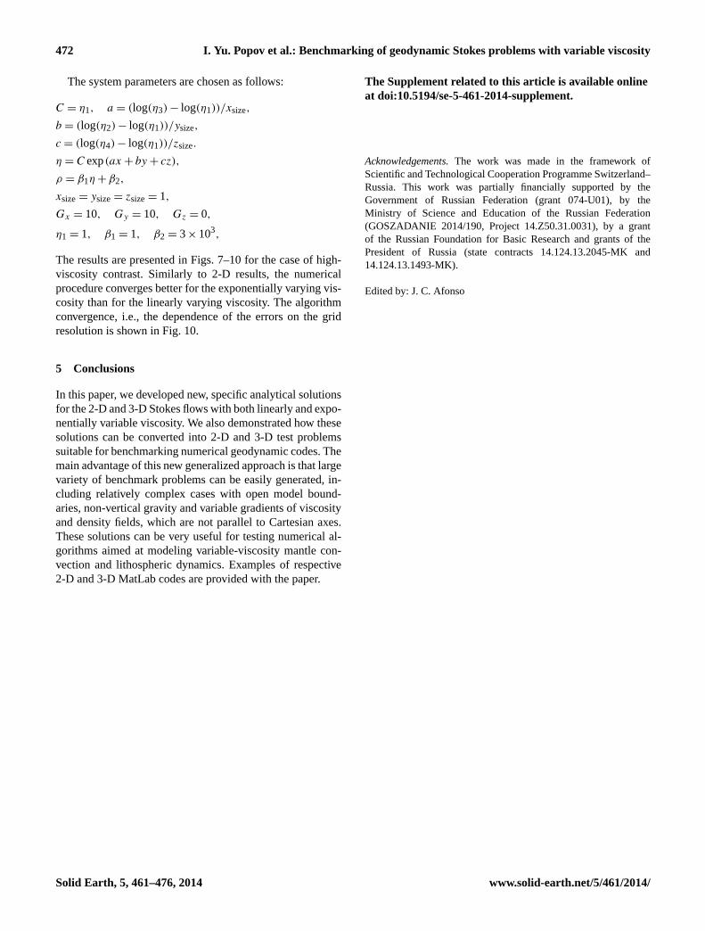
The system parameters are chosen as follows:

C = η1, a = (log(η3) − log(η1))/xsize,

b = (log(η2) − log(η1))/ysize,

c = (log(η4) − log(η1))/zsize.

η = C exp(ax + by + cz),

ρ = β1η + β2,

xsize= ysize= zsize= 1,

Gx = 10, Gy = 10, Gz = 0,

η1 = 1, β1 = 1, β2 = 3× 103,

The results are presented in Figs. 7–10 for the case of high-viscosity contrast. Similarly to 2-D results, the numericalprocedure converges better for the exponentially varying vis-cosity than for the linearly varying viscosity. The algorithmconvergence, i.e., the dependence of the errors on the gridresolution is shown in Fig. 10.

5 Conclusions

In this paper, we developed new, specific analytical solutionsfor the 2-D and 3-D Stokes flows with both linearly and expo-nentially variable viscosity. We also demonstrated how thesesolutions can be converted into 2-D and 3-D test problemssuitable for benchmarking numerical geodynamic codes. Themain advantage of this new generalized approach is that largevariety of benchmark problems can be easily generated, in-cluding relatively complex cases with open model bound-aries, non-vertical gravity and variable gradients of viscosityand density fields, which are not parallel to Cartesian axes.These solutions can be very useful for testing numerical al-gorithms aimed at modeling variable-viscosity mantle con-vection and lithospheric dynamics. Examples of respective2-D and 3-D MatLab codes are provided with the paper.

The Supplement related to this article is available onlineat doi:10.5194/se-5-461-2014-supplement.

Acknowledgements.The work was made in the framework ofScientific and Technological Cooperation Programme Switzerland–Russia. This work was partially financially supported by theGovernment of Russian Federation (grant 074-U01), by theMinistry of Science and Education of the Russian Federation(GOSZADANIE 2014/190, Project 14.Z50.31.0031), by a grantof the Russian Foundation for Basic Research and grants of thePresident of Russia (state contracts 14.124.13.2045-MK and14.124.13.1493-MK).

Edited by: J. C. Afonso


http://dx.doi.org/10.5194/se-5-461-2014-supplement


Appendix A: Error decreasing with decreasing grid res-olution

The dependence of the convergence on the viscosity con-trast is shown in the following tables. Namely, the viscosi-tiesη2,η3 run through a set of values from 2 to 10000. Foreach pair ofη2,η3 we perform the benchmarking proceduredescribed above and obtain the curve describing the depen-dence of the logarithm of the error norm on the logarithmof the grid resolution. The tangent of the slope angle of thiscurve gives us an input of the table. Full set of tables aregiven in the Supplement. Below, we show several examplesof such tables.

Table A1.Tangent of the slope of the curve showing the dependenceof the logarithm ofL2-error for pressureP on the logarithm of thegrid step for different viscosity contrasts. Linearly varying viscosity.

η2 2 5 20 100 300 1000 10 000η3

2 1.42 1.14 1.24 0.86 0.46 0.08 −0.205 1.13 1.44 1.03 1.30 0.57 0.23 −0.1620 1.23 1.03 1.39 1.27 0.83 0.43 −0.01100 1.14 1.21 1.26 1.36 1.33 0.50 0.26300 1.27 1.27 1.29 1.33 1.34 1.17 0.401000 0.56 0.70 1.03 1.24 1.31 1.36 0.3910 000 −0.21 −0.19 −0.04 0.23 0.34 0.43 1.27

Table A2. Tangent of the slope of the curve showing the depen-dence of the logarithm ofL2-error for velocity componentvx onthe logarithm of the grid step for different viscosity contrasts. Lin-early varying viscosity.

η2 2 5 20 100 300 1000 10 000η3

2 1.81 1.99 1.81 1.20 0.70 0.29 0.015 1.53 1.61 1.80 1.79 0.91 0.47 0.0420 1.47 1.54 1.61 1.81 1.09 0.77 0.20100 1.13 1.39 1.54 1.69 2.04 0.94 0.53300 1.64 1.63 1.63 1.61 1.70 1.49 0.771000 0.56 0.77 1.23 1.57 1.60 1.15 0.9010 000 −0.19 −0.13 0.01 0.41 0.69 0.96 0.88

Table A3. Tangent of the slope of the curve showing the depen-dence of the logarithm ofL2-error for velocity componentvy onthe logarithm of the grid step for different viscosity contrasts. Lin-early varying viscosity.

η2 2 5 20 100 300 1000 10 000η3

2 1.99 1.53 1.49 1.14 0.51 0.07 −0.215 1.99 1.90 1.54 1.61 0.79 0.26 −0.1920 1.81 1.80 1.79 1.56 1.24 0.63 −0.03100 1.27 1.47 1.79 2.03 1.61 0.94 0.34300 1.86 1.93 1.99 2.04 2.04 1.43 0.601000 0.37 0.53 0.90 1.56 1.97 2.03 0.7410 000 0.019 0.04 0.20 0.54 0.76 0.89 1.23

A1 Linearly varying viscosity

Tables A1–A3 contain log rates ofL2 error norm decreasingwith decreasing grid resolution (the curve slope in Fig. 3 inthe logarithmic scale) for different viscosity contrasts in thecase of linearly varying viscosity. Calculations were madefor the following system parameters:

xsize= ysize= 1, Gx = 0, Gy = 10,

η1 = 1, β1 = 102, β2 = 3× 103,

c = η1, a = (η3 − η1)/xsize, b = (η2 − η1)/ysize,

ρ = β1(ax + by + c) + β2.



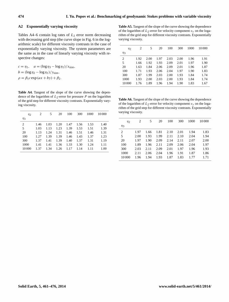
A2 Exponentially varying viscosity

Tables A4–6 contain log rates ofL2 error norm decreasingwith decreasing grid step (the curve slope in Fig. 6 in the log-arithmic scale) for different viscosity contrasts in the case ofexponentially varying viscosity. The system parameters arethe same as in the case of linearly varying viscosity with re-spective changes:

c = η1, a = (logη3 − logη1)/xsize,

b = (logη2 − logη1)/ysize,

ρ = β1cexp(ax + by) + β2.

Table A4. Tangent of the slope of the curve showing the depen-dence of the logarithm ofL2-error for pressureP on the logarithmof the grid step for different viscosity contrasts. Exponentially vary-ing viscosity.

η2 2 5 20 100 300 1000 10 000η3

2 1.46 1.03 1.20 1.47 1.56 1.53 1.405 1.03 1.13 1.23 1.39 1.53 1.51 1.3920 1.13 1.24 1.31 1.46 1.51 1.46 1.31100 1.27 1.39 1.39 1.46 1.43 1.37 1.23300 1.37 1.41 1.39 1.40 1.37 1.31 1.191000 1.41 1.41 1.36 1.33 1.30 1.24 1.1110 000 1.37 1.34 1.26 1.17 1.14 1.11 1.00

Table A5.Tangent of the slope of the curve showing the dependenceof the logarithm ofL2-error for velocity componentvx on the loga-rithm of the grid step for different viscosity contrasts. Exponentiallyvarying viscosity.

η2 2 5 20 100 300 1000 10 000η3

2 1.92 2.00 1.97 2.03 2.00 1.96 1.915 1.66 1.92 1.93 2.09 2.01 1.97 1.9020 1.63 1.84 2.06 2.09 2.01 1.96 1.87100 1.71 1.93 2.06 2.04 1.97 1.90 1.83300 1.87 1.99 2.03 2.00 1.93 1.84 1.741000 1.93 2.00 2.03 2.00 1.93 1.84 1.7410 000 1.76 1.89 1.96 1.94 1.90 1.83 1.67

Table A6.Tangent of the slope of the curve showing the dependenceof the logarithm ofL2-error for velocity componentvy on the loga-rithm of the grid step for different viscosity contrasts. Exponentiallyvarying viscosity.

η2 2 5 20 100 300 1000 10 000η3

2 1.97 1.66 1.81 2.10 2.01 1.94 1.835 2.00 1.93 1.99 2.11 2.10 2.04 1.9420 1.97 1.90 2.09 2.14 2.11 2.07 2.00100 1.89 1.96 2.11 2.09 2.06 2.04 1.97300 2.03 2.11 2.09 2.01 1.97 1.96 1.931000 2.11 2.06 2.04 1.96 1.91 1.87 1.8610 000 1.96 1.94 1.93 1.87 1.83 1.77 1.71



References

Albers, M.: A local mesh refinement multigrid method for 3-D con-vection problems with strongly variable viscosity, J. Comput.Phys., 160, 126–150, 2000.

Blankenbach, B., Busse, F., Christensen, U. Cserepes, L., Gunkel,D., Hansen, U., Harder, H., Jarvis, G., Koch, M., Marquart,G., Moore, D., Olson, P., Schmeling H., and Schnaubelt, T.:A benchmark comparison for mantle convection codes, Geophys.J. Int., 98, 23–38, 1989.

Buiter, S. J. H., Babeyko, A. Y., Ellis, S., Gerya, T. V., Kaus, B. J. P.,Kellner, A., Schreurs, G., and Yamada, Y.: The numerical sand-box: comparison of model results for a shortening and an ex-tension experiment, in: Analogue and Numerical Modelling ofCrustal-Scale Processes, Geol. Soc., London, Special Publica-tions, 253, 29–64, 2006.

Busse, F. H., Christensen, U., Clever, R., Cserepes, L., Gable, C.,Giannandrea, E., Guillon, L., Houseman, G., Nataf, H.-C.,Ogawa, M., Parmentier, M., Sotin, C., and Travis, B.: 3-Dconvection at infinite Prandtl number in Cartesian geometry –a benchmark comparison, Geophys. Astro. Fluid, 75, 39–59,1993.

Crameri, F., Schmeling, H., Golabek1, G. J., Duretz, T., Orendt, R.,Buiter, S. J. H., May, D. A., Kaus, B. J. P., Gerya, T. V., and Tack-ley, P. J.: A comparison of numerical surface topography calcula-tions in geodynamic modelling: an evaluation of the “sticky air”method, Geophys. J. Int., 189, 38–54, 2012.

Dabrowski, M., Krotkiewski, M., and Schmid, D. W.: MIL-AMIN: MATLAB-based finite-element method solver forlarge problems, Geochem. Geophy. Geosy., 9, Q04030,doi:10.1029/2007GC001719, 2008.

Deubelbeiss, Y. and Kaus, B. J. P.: Comparison of Eulerian and La-grangian numerical techniques for the Stokes equations in thepresence of strongly varying viscosity, Phys. Earth Planet. In.,171, 92–111, 2008.

Duretz, T., May, D. A., Gerya, T. V., and Tackley, P. J.: Dis-cretization errors and free surface stabilization in the finitedifference and marker-in-cell method for applied geodynam-ics: a numerical study, Geochem. Geophy. Geosy., 12, Q07004,doi:10.1029/2011GC003567, 1–26, 2011.

Gerya, T.: Introduction to Numerical Geodynamic Modelling, Cam-bridge University Press, Cambridge, 2010.

Gerya, T. V. and Yuen, D. A.: Characteristic-based marker-in-cellmethod with conservative finite-difference schemes for model-ing geological flows with strongly variable transport properties,Phys. Earth Planet. In., 140, 293–318, 2003.

Gerya, T. V. and Yuen, D. A.: Robust characteristics methodfor modeling multiphase visco-elasto-plastic thermo-mechanicalproblems, Phys. Earth Planet. In., 163, 83–105, 2007.

Gerya, T. V., May, D. A., and Duretz, T.: An adaptive staggered gridfinite difference method for modeling geodynamic Stokes flowswith strongly variable viscosity, Geochem. Geophy. Geosy., 14,1200–1225, 2013.

Hager, B. H. and O’Connell, R. J.: A simple global model of planedynamics and mantle convection, J. Geophys. Res., 86, 4843–4867, 1981.

Ismail-Zadeh, A. and Tackley, P.: Computational Methods in Geo-dynamics, Cambridge University Press, Cambridge, 2010.

Kaus, B. J. P.: Factors that control the angle of shear bands in geody-namic numerical models of brittle deformation, Tectonophysics,484, 36–47, 2010.

Kaus, B. J. P. and Becker, T. W.: Effects of elasticity on theRayleigh–Taylor instability: implications for large-scale geody-namics, Geophys. J. Int., 168, 843–862, 2007.

Kaus, B. J. P. and Schmalholz, S. M.: 3-D Finite amplitudefolding: implications for stress evolution during crustal andlithospheric deformation, Geophys. Res. Lett., 33, L14309,doi:10.1029/2011GC003567, 2006.

Lemiale, V., Muhlhaus, H.-B., Moresi, L. and Stafford, J.: Shearbanding analysis of plastic models formulated for incompress-ible viscous flows, Phys. Earth Planetary Interiors, 171, 177–186,2008.

Lobanov, I. S., Popov, I. Yu., Popov, A. I., and Gerya, T. V.: Nu-merical approach to the Stokes problem with high contrasts inviscosity, Appl. Mathemat. Comput., 235, 17–25, 2014.

Moresi, L., Zhong, S., and Gurnis, M.: The accuracy of finite ele-ment solutions of Stokes’ flow with strongly varying viscosity,Phys. Earth Planet. In., 97, 83–94, 1996.

Moresi, L., Dufour, F., and Mulhaus, H.-B.: A Lagrangian integra-tion point finite element method for large deformation modelin-gof viscoelastic geomaterials, J. Comput. Phys., 184, 476–497,2003.

Popov, A. and Sobolev, S.: SLIM3D: a tool for three-dimensionalthermomechanical modeling of lithospheric deformation withelasto-visco-plastic rheology, Phys. Earth Planet. In., 171, 55–75, 2008.

Popov, I. Yu. and Makeev, I. V.: A benchmark solution for 2-DStokes flow over cavity, Z. Angew. Math. Phys., 65, 339–348,2014.

Ramberg, H.: Instability of layered system in the field of gravity, II,Phys. Earth Planet. In., 1, 448–474, 1968.

Revenaugh, J. and Parsons, B.: Dynamic topography and gravityanomalies for fluid layers whose viscosity varies exponentiallywith depth, Geophys. J. Int., 90, 349–368, 1987.

Schmeling, H., Babeyko, A. Y., Enns, A., Faccenna, C., Funi-ciello, F., Gerya, T. V., Golabek, G. J., Grigull, S., Kaus, B. J. P.,Morra, G., Schmalholz, S. M., and van Hunen, J.: A benchmarkcomparison of spontaneous subduction models – towards a freesurface, Phys. Earth Planet. In., 171, 198–223, 2008.

Schmid, D. V. and Podladchikov, Yu. Yu.: Analytical solutions fordeformable elliptical inclusions in general shear, Geophys. J. Int.,155, 269–288, 2003.

Stadler, G., Gurnis, M., Burstedde, C., Wilcox, L. C., Alisic, L., andGhattas, O.: The dynamics of plate tectonics and mantle flow:from local to global scales, Science, 329, 1033–1038, 2008.

Tackley, P. J.: Modelling compressible mantle convection with largeviscosity contrasts in a three-dimensional spherical shell usingthe yin-yang grid, Phys. Earth Planet. In., 171, 7–18, 2008.

Tackley, P. J. and King, S. D.: Testing the tracer ratio method-for modeling active compositional fields in mantle con-vection simulations, Geochem. Geophy. Geosys., 4, 8302,doi:10.1029/2001GC000214, 2003.

Thieulot, C.: FANTOM: two- and three-dimensional numericalmodelling of creeping flows for the solution of geological prob-lems, Phys. Earth Plane. Int., 188, 47–68, 2011.

Thieulot, C., Fullsack, P. and Braun, J. Adaptive octree-basedfinite element analysis of two- and three-dimensional


http://dx.doi.org/10.1029/2007GC001719

http://dx.doi.org/10.1029/2011GC003567

http://dx.doi.org/10.1029/2011GC003567

http://dx.doi.org/10.1029/2001GC000214


indentation problems, J. Geophys. Res., 113, B12207,doi:10.1029/2008JB005591, 2008.

Torrance, K. E. and Turcotte, D. L.: Thermal convection with largeviscosity variations, J. Fluid Mech., 47, 113–125, 1971.

Turcotte, D. L. and Schubert, G.: Geodynamics, Cambridge Univer-sity Press, Cambridge, 2002.

van Keken, P. E., King, S. D., Schmeling, H., Christensen, U. R.,Neumeister, D., and Doin, M.-P.: A comparison of methods forthe modeling of thermochemical convection, J. Geophys. Res.-Sol. Earth., 102, 22477–22495, 1997.

van Keken, P. E., Currie, C., King, S. D., Behn, M. D., Cangleon-cle, A., He, J., Katz, R. F., Lin, S.-C., Parmentier, E. M., Spiegel-man, M., and Wang, K.: A community benchmark for subductionzone modeling, Phys. Earth Planet. In., 171, 187–197, 2008.

Zhong, S.: Analytic solutions for Stokes flow with lateral variationsin viscosity, Geophys. J. Int., 124, 18–28, 1996.

Zhong, S. and Gurnis, M.: The role of plates and temperature-dependent viscosity in phase change dynamics, J. Geophys. Res.,99, 15903–15917, 1994.

Zhong, S., McNamara, A., Tan, E., Moresi, L., and Gurnis, M.:A benchmark study on mantle convection in a 3-D sphericalshell using CitcomS, Geochem. Geophy. Geosy., 9, Q10017,doi:10.1029/2008GC002048, 2008.


http://dx.doi.org/10.1029/2008JB005591

http://dx.doi.org/10.1029/2008GC002048

practical analytical solutions for benchmarking of 2 … · practical analytical solutions for...

Documents