pr - colorado state university
TRANSCRIPT

PROJECT REPORT
USING NEURAL NETWORKS FOR APPROXIMATE RADIOSITY FORM FACTOR
COMPUTATION
Submitted by
Charles Martin
Department of Computer Science
In partial ful�llment of the requirements
for the degree of Master of Science
Colorado State University
Fort Collins, Colorado
Summer, 1996

ABSTRACT OF PROJECT REPORT
USING NEURAL NETWORKS FOR APPROXIMATE RADIOSITY FORM FACTOR
COMPUTATION
Radiosity is a method used in computer graphics to compute the distribution of di�use
illumination within a scene. The largest cost of rendering a scene with radiosity is the
computation of geometrical relationships, called form factors, between each pair of objects
within the scene. This project report explores the use of neural networks to accelerate the
computation of radiosity form factors.
Charles Martin
Department of Computer Science
Colorado State University
Fort Collins, Colorado 80523
Summer, 1996
ii

CONTENTS
1 Introduction 1
1.1 Overview : : : : : : : : : : : : : : : : : : : : : : : : : : : : : : : : : : : : : : : 1
1.2 Radiosity : : : : : : : : : : : : : : : : : : : : : : : : : : : : : : : : : : : : : : : 1
1.3 Approximation with Neural Networks : : : : : : : : : : : : : : : : : : : : : : : 2
1.4 Outline of Project Report : : : : : : : : : : : : : : : : : : : : : : : : : : : : : : 3
2 Radiosity Concepts 4
2.1 Overview : : : : : : : : : : : : : : : : : : : : : : : : : : : : : : : : : : : : : : : 4
2.2 De�nition of Radiosity : : : : : : : : : : : : : : : : : : : : : : : : : : : : : : : : 4
2.3 The Radiosity Equation : : : : : : : : : : : : : : : : : : : : : : : : : : : : : : : 5
2.4 Form Factors : : : : : : : : : : : : : : : : : : : : : : : : : : : : : : : : : : : : : 7
2.5 Computations Subsequent to Form Factor Calculations : : : : : : : : : : : : : 8
2.6 The Hemicube Approximation : : : : : : : : : : : : : : : : : : : : : : : : : : : 8
2.7 An Analytic Solution : : : : : : : : : : : : : : : : : : : : : : : : : : : : : : : : : 12
2.8 Training the Neural Networks with Cross Validation : : : : : : : : : : : : : : : 13
2.9 Comparing the Complexities of the Hemicube and Neural
Network Methods : : : : : : : : : : : : : : : : : : : : : : : : : : : : : : : : : 13
2.10 Summary : : : : : : : : : : : : : : : : : : : : : : : : : : : : : : : : : : : : : : : 15
3 Experiments with Random Data 16
3.1 Overview : : : : : : : : : : : : : : : : : : : : : : : : : : : : : : : : : : : : : : : 16
3.2 Generating Data : : : : : : : : : : : : : : : : : : : : : : : : : : : : : : : : : : : 16
3.3 The Neural Network : : : : : : : : : : : : : : : : : : : : : : : : : : : : : : : : : 17
3.4 The Experiment : : : : : : : : : : : : : : : : : : : : : : : : : : : : : : : : : : : 18
3.5 Results : : : : : : : : : : : : : : : : : : : : : : : : : : : : : : : : : : : : : : : : 20
4 Experiments with Data From a Simple Scene 24
4.1 Overview : : : : : : : : : : : : : : : : : : : : : : : : : : : : : : : : : : : : : : : 24
4.2 The Method : : : : : : : : : : : : : : : : : : : : : : : : : : : : : : : : : : : : : : 24
4.2.1 Modifying Rad : : : : : : : : : : : : : : : : : : : : : : : : : : : : : : : : : : : 24
4.2.2 Data Generation : : : : : : : : : : : : : : : : : : : : : : : : : : : : : : : : : : 26
4.2.3 Training the Neural Networks : : : : : : : : : : : : : : : : : : : : : : : : : : : 28
4.2.4 Evaluation : : : : : : : : : : : : : : : : : : : : : : : : : : : : : : : : : : : : : 28
4.3 Results : : : : : : : : : : : : : : : : : : : : : : : : : : : : : : : : : : : : : : : : 29
4.3.1 Statistical Results : : : : : : : : : : : : : : : : : : : : : : : : : : : : : : : : : 29
4.3.2 Visual Results : : : : : : : : : : : : : : : : : : : : : : : : : : : : : : : : : : : 30
iii

5 Conclusion 34
5.1 Visibility : : : : : : : : : : : : : : : : : : : : : : : : : : : : : : : : : : : : : : : 34
5.2 Representation of the Patches : : : : : : : : : : : : : : : : : : : : : : : : : : : : 35
5.3 Future Work : : : : : : : : : : : : : : : : : : : : : : : : : : : : : : : : : : : : : 36
6 REFERENCES 37
iv

LIST OF FIGURES
1.1 The Geometrical Relationships Between Elements in Form Factor Calculations 2
2.1 De�nition of radiance. : : : : : : : : : : : : : : : : : : : : : : : : : : : : : : : 5
2.2 Radiosity notation. : : : : : : : : : : : : : : : : : : : : : : : : : : : : : : : : : 6
2.3 Nussult's analogy. : : : : : : : : : : : : : : : : : : : : : : : : : : : : : : : : : : 10
2.4 The Hemicube. : : : : : : : : : : : : : : : : : : : : : : : : : : : : : : : : : : : 11
2.5 Computation of the delta-form factors. : : : : : : : : : : : : : : : : : : : : : : 11
2.6 A feed-forward neural network. : : : : : : : : : : : : : : : : : : : : : : : : : : : 14
3.1 A schematic of the experiment with randomly generated data. : : : : : : : : : 19
4.1 The algorithm for neural net and analytic form factor calculations. : : : : : : : 25
4.2 Experiment Design : : : : : : : : : : : : : : : : : : : : : : : : : : : : : : : : : : 27
4.3 A simple radiosity scene rendered with the analytic, hemicube and neural net-
work methods. : : : : : : : : : : : : : : : : : : : : : : : : : : : : : : : : : : 31
v

LIST OF TABLES
3.1 Results of neural net (NN) and hemicube (HC) calculations on randomly gen-
erated data. : : : : : : : : : : : : : : : : : : : : : : : : : : : : : : : : : : : : 21
3.2 All Data Sets Concatenated and then Binned by Decade : : : : : : : : : : : : : 22
4.1 Results of rendering a simple scene with various neural networks. : : : : : : : : 29
vi

Chapter 1
INTRODUCTION
1.1 Overview
In the quest for greater realism in computer graphics, increasingly complex illumi-
nation methods are being used to model not only the light falling directly on an object,
but also the light re ected from other objects in the scene. The realism provided by these
methods comes at the cost of greater computational complexity.
Radiosity is a method which computes the distribution of light from di�use sources
and di�use re ectors in a scene. The largest cost involved in rendering a scene with
radiosity is in the computation of geometrical relationships, called form factors, between
sections of the surfaces within the scene. This project report explores the use of neural
networks to accelerate the computation of radiosity form factors.
1.2 Radiosity
Radiosity is a method of calculating the distribution of di�use illumination within
a scene. In this method, every surface in the scene is divided into patches. Then, for
each patch, the contribution of light from every other patch in the scene is calculated and
summed into the total amount of light impinging on the patch. This redistribution of light
is repeated until the distribution of light in the scene stabilizes.
The contribution of illumination from one patch on another depends purely on geo-
metric considerations. For each pair of patches, a form factor is calculated which indicates
the relative amount of radiation from one patch to the other. The form factor, Fij , from
patch Ai to Aj can be expressed as
Fij =1
Ai
ZAi
ZAj
cos �i cos �j
�r2dAi dAj ; (1.1)

2
where �i and �j are the angles between the normals of the di�erential elements dAi and
dAj and ~r is the vector between the centers of two di�erential elements. Figure 1 illustrates
the geometrical relationships in form factor calculations. Although closed form solutions
r
N
Θ
j
AdA
Θ N
A
dA
i
i
i
i
j j
j
Figure 1.1: The Geometrical Relationships Between Elements in Form Factor Calculations
exist for simple geometries, no general closed form solution exits.
1.3 Approximation with Neural Networks
Since the above integral has no general closed form solution, a number of approximate
schemes have been developed. These methods are computationally expensive and represent
the major bottleneck in the computation of radiosity calculations. Fast approximations of
the form factors would allow considerably faster computation of radiosity calculations and
would allow these computations to take place with less hardware than currently required.

3
Neural networks have a well known role as \function approximators" and were used in
this project to calculate radiosity form factors.
The overall goal of this project is to determine whether or not a neural network can
be trained to provide a useful approximation of radiosity form factors. Since no general
closed form solution to equation 1.1 above exists, the reduced problem of calculating form
factors for planar quadrilaterals will be considered. Schr�oder and Hanrahan [Schro 93]
have published a closed form solution for form factor calculation for general polygons and
have made a C library available for its computation. This solution will be used to train
and test the accuracy of the neural network approximation.
Since the analytic solution calculated by the C library is quite slow, the most popular
form factor approximation method, the hemicube, will also be run on the same data as a
measure of acceptable accuracy.
Two sets of data were generated. The �rst is a set of random, planar quadrilaterals
for which the analytic and hemicube approximations were computed. A neural network
was trained on the data with the values computed by the analytic solution as target
values. The trained network was then run on the same data to see how accurately it could
reproduce the form factor values and these results were compared to both the analytic
solution and the hemicube solution. The second set of data was from a simple scene and
was generated with a modi�ed radiosity rendering program. The form factor values were
computed with the analytic solution and a series of neural networks was trained. The
scene was rendered again with the neural network and the resulting form factor values
were compared with the analytic solution and the neural network solution.
1.4 Outline of Project Report
The following chapters will discuss the mathematical underpinnings of radiosity, the
methods used to train the neural network and the results of applying the neural network
to a simple scene. Chapter 2 describes radiosity form factors and the mathematics behind
them. Chapter 3 describes the experiments with random data. Chapter 4 describes the
experiments with data from a graphics scene. Chapter 5 concludes the report and suggests
future directions for research.

Chapter 2
RADIOSITY CONCEPTS
2.1 Overview
Radiosity describes the distribution of radiative energy in an environment. This
chapter introduces the basics of the radiosity method, the derivation of form factors
and describes the hemicube and neural network schemes for approximate computation of
form factors. The relative complexity of these approximation schemes will be compared.
More complete and general treatments of radiosity are given in heat transfer texts such
as [Sparr 78]. We use the notation used in Sillion's book [Sill 94] and use the development
in pages 9-13 and 23-31.
2.2 De�nition of Radiosity
Radiance, L, is de�ned as the amount of energy traveling at some point in a speci-
�ed direction per unit time, per unit area perpendicular to the direction of travel. (See
Figure 2.1.) Thus, the energy radiated into d! from dx2 in time dt is
L(x; �; �) dx cos � d!dt:
Hence, the power radiated into d! from dx2 is
d2P = L(x; �; �) dx cos � d!:
A useful property of radiance, which we won't derive, is the following reciprocity
property. For two points x and y, which are mutually visible
L(x; �x; �x) = L(y; �y; �y):

5
Figure 2.1: De�nition of radiance.
(From [Sill 94, page 9]).
Radiosity, B(x), is de�ned as the total power leaving a point, x, on a surface per unit
area on the surface
B(x) =dP
dx=
Z
L(x; �; �) cos �d! (2.1)
where means integration over the hemisphere above the patch.
2.3 The Radiosity Equation
Equation 2.1 is a general expression which characterizes the total radiation leaving
a point on a surface. However, radiosity as used in computer graphics makes some sim-
plifying assumptions. First, the environment in computer graphics is closed. Hence, all
radiation leaving a given surface in the environment will be received by another surface
in the environment; radiation from a surface will not sail o� into \deep space". Second,
ideal di�use re ectors are assumed which implies that L is independent of angle. Hence,
L(x; �; �) = L(x):
We next seek to consider the distribution of energy from the point of view of a point
on a surface. Energy radiating from the point can be considered to be the sum of two

6
Figure 2.2: Radiosity notation.
(From [Sill 94, page 29].)
sources. If a point is an emitter then it radiates light into the environment as a source.
The point can also gather radiation from the environment and re-radiate it into the scene
through di�use re ectance. This can be written
B(x) = E(x) + �(x)H(x);
where E(x) is the total power emitted by the point (as a source) per unit area, �(x) is the
re ectivity at point x and H(x) is the total power impinging on the surface per unit area.
Using the properties of ideal di�use re ectors and the reciprocity property of radiance
mentioned above, it can be shown [Sill 94, pg. 26] that
H(x) =1
�
Zy2S
B(y)cos � cos �
0
�r2V (x; y)dy;
where S is the surface of integration, � and �0
are de�ned in Figure 2.2 and
V (x; y) =
(1; if x and y are mutually visible;
0; otherwise.

7
Thus our energy balance equation can be written
B(x) = E(x) + �(x)1
�
Zy2S
B(y)cos � cos �
0
�r2V (x; y)dy; (2.2)
which is the radiosity equation for the continuous case.
2.4 Form Factors
In practice we need a discrete formulation of Equation 2.2 in order to render an
environment. Most common radiosity methods use some sort of meshing scheme to divide
the surfaces in the environment into patches and we would like to be able to compute
average radiosity values for each patch.
We can discretize 2.2 in a straightforward manner assuming an average radiosity
across patches:
B(x) = E(x) + �(x)NXj=1
Bj
Zy2Pj
cos � cos �0
�r2V (x; y)dy; (2.3)
where Bj is the area-weighted average of the radiosity across patch Pj
Bj =1
Aj
Zx2Pj
B(x)dx:
Similarly, the energy emitted from the patch as a source (not through re ectance) can be
written as
Ej =1
Aj
Zx2Pj
E(x)dx:
Finally, to compute Bi, we assume an average re ectivity, �i and then we can take an
area-weighted average of Equation 2.3 to compute
Bi = Ei + �i
nXj=1
Bj
1
Ai
Zx2Pi
Zy2Pj
cos � cos �0
�r2V (x; y)dydx:
We can write this equation more simply as
Bi = Ei + �i
nXj=1
FijBj; (2.4)
where
Fij =1
Ai
Zx2Pi
Zy2Pj
cos � cos �0
�r2V (x; y)dydx: (2.5)
The term Fij is known as the form factor between patch Pi and patch Pj and it
describes the proportion of total power leaving patch Pi that is received by patch Pj .
There is no known general closed form solution to the double integral in Equation 2.5.

8
2.5 Computations Subsequent to Form Factor Calculations
Although computation of the form factors describes the geometrical relationships
between patches in a scene, it does not describe the distribution of light in the scene.
Each of the n patches in a scene has a corresponding instance of Equation 2.4. These
equations must be solved simultaneously in order to describe the distribution of light
within a scene. These equations can be written as a matrix equation:
0BBBB@
B1
B2
...
Bn
1CCCCA =
0BBBB@
E1
E2
...
En
1CCCCA+
0BBBBB@
�1F11 �1F12 � � � �1F1n
�2F21 �2F22...
......
�nFn1 �nFn2 �nFnn
1CCCCCA
0BBBB@
B1
B2
...
Bn
1CCCCA
or rewritten as0BBBBB@
1� �1F11 ��1F12 � � � ��1F1n
��2F21 1� �2F22...
......
��nFn1 ��nFn2 1� �nFnn
1CCCCCA
0BBBB@
B1
B2
...
Bn
1CCCCA =
0BBBB@
E1
E2
...
En
1CCCCA :
Solving the above equation is a familiar problem and many iterative methods exist to
invert the matrix on the left hand side of the equation. For scenes in which the number
of patches is relatively small, Gauss-Seidel relaxation can be used. For scenes with a large
number of patches, hybrids of Southwell and Jacobi iteration (progressive radiosity) are
frequently used. (See chapter 5 in [Cohen 93].)
2.6 The Hemicube Approximation
Given that there is no closed form solution to Equation 2.5, some form of approxima-
tion has to be made to compute form factors. The hemicube is one of the most popular
approximation method used in radiosity form factor computation. Despite the fact that
its accuracy is limited, its speed makes it the most popular choice.
The hemicube approximation rests on two assumptions. The �rst is that the inner
integral of Equation 2.5 varies little across the surface of patch Pi. Thus the area weighted
product of the outer integral can be approximated by a single di�erential element:
Fij =1
Ai
Zx2Pi
Zy2Pj
cos � cos �0
�r2V (x; y)dydx �
Zy2Pj
cos � cos �0
�r2V (x; y)dy: (2.6)

9
This is a valid assumption provided the squared distance between the patches is larger
than the area of the patches. However, since we've already constrained the problem to
a closed environment, it will be likely that a number of the patches in the scene will be
closer to each other than this approximation assumes.
The second approximation used is Nusselt's analogy which is a geometrical interpre-
tation of the form factor (Figure 2.3). The value of the form factor is the ratio of the
intersection of the solid angle and the unit hemisphere projected on to the plane of the
patch and the area of the unit circle. This implies that all patches which intersect the
same solid angle will have the same form factor value.
The hemicube method erects a meshed half-cube above the center of the gathering
patch and pre-computes the form factor value for each window in the mesh. The form
factor values for each window are called delta form factors The hemicube method then
shoots a ray from the center of the gathering patch through the center of the window and
records the patch number of the closest patch intersecting the ray. After shooting a ray,
the form factor value between the gathering patch and the closest patch for that window
is incremented by the contribution to the form factor value for that window (Figure 2.4).
Because this method is similar to depth bu�ering algorithms used for rendering a scene,
the hemicube method is able to make use of special purpose hardware for depth bu�er
calculations built into many graphics cards in order to further accelerate the computation
of form factors.
Because of the simplicity of the geometry of the hemicube, computation of the delta
form factors is quite simple (Figure 2.5). Rewriting Equation 2.6 from a point x to a patch
P we have
Fx;P =1
�
ZP
cos � d!
where P is the set of directions in which a point on P is visible from x. Since
d! ��A cos �
r2;
the top faces of the hemicube (of unit height) have delta form factor values
�F =�A
�(1 + x2 + y2)2(2.7)

10
Figure 2.3: Nussult's analogy.
(From [Sill 94, page 49].)

11
Figure 2.4: The Hemicube.
(From [Sill 94, page 51].)
Figure 2.5: Computation of the delta-form factors.
(From [Sill 94, page 51].)

12
and the side faces (positioned a unit from the origin) have delta form factor values of
�F =�A
�(1 + z2 + y2)2(2.8)
for a hemicube with a top face of 2 by 2 units and sides 1 unit tall.
There are several well known errors in the hemicube method. The most obvious error
is aliasing caused by the �xed number of windows in the hemicube. If the hemicube has n
windows in an environment having N patches and if n < N then obviously the hemicube
cannot gather light from all patches in the scene even if they are all visible. Thus it is
possible for a patch to miss a contribution from a light source while its neighboring patch
might include the contribution from that patch. These discontinuities in sampling cause
banding in the intensity of the �nal image. A second error in the hemicube method is
the lack of accuracy when patches are close together caused by the assumption that the
value of the inner integral does not vary much across the gathering patch. Although the
numerical values computed by the hemicube method for patches close together may be
100% or more o� from the true values, these errors do not produce discontinuities because
they are mis-approximations of geometrical relationships rather than computational noise.
Hence, they are less visible in the �nal image than aliasing errors.
Because the hemicube is so widely used in rendering radiosity images, it makes an
excellent benchmark for the usability of other form factor calculation methods and was
used to measure the usefulness of the neural network approximation.
2.7 An Analytic Solution
In 1993 Schr�oder and Hanrahan [Schro 93] published a closed form solution for the
computation of form factors between two general (planar, convex or concave, perhaps
containing holes) polygons. They made a C library implementation available over the
internet from Princeton University. (See reference [Schro 93]). The library functions
calculate the form factor between two polygons which are speci�ed by lists of the x; y; and
z values of each vertex in each polygon.
This library is too slow to be of practical use for rendering and the authors themselves
state the principle use of the library is for the computation of reference solutions for

13
other, faster, approximation methods. The library is also somewhat fragile because of its
extensive use of inverse trigonometric functions, but we were able to use it as a ground
truth for the accuracy of both the hemicube and the neural network approximation. The
library consists of about 1300 lines of C code. The analytic solution itself requires the
computation of four auxiliary functions each of which require the solution of an integral.
The �nal solution has eighteen constants of integration. If nothing else, the complexity of
the solution is a testament to the di�culty of solving the form factor integral.
2.8 Training the Neural Networks with Cross Validation
The neural networks were trained using backpropagation with cross validation [Hass 95,
page 226]. Using cross validation makes the training more resistant to over �tting of the
training data. Roughly 80% of the training data was used to train the neural network,
10% was used as a validation set and 10% was used as a test set. With this method,
backpropagation is performed with the training set. The update rule in the method used
here seeks to minimize squared error over the training set. After an epoch of training,
the mean squared error of running the network on the validation set is computed. If the
validation error is lower than the current best validation error, then the weights of the
nodes in the neural network are saved. The test data set is also applied to the neural
network after each epoch in order to test how well the neural network will be able to
generalize to data it hasn't trained on.
The input vector for the neural networks was a list of the x; y and z values of each
vertex of each polygon. This representation of the input data, while simplistic, matches
that used by the analytic form factor library. This representation also has the advantage
of being easily extracted from graphics rendering software.
2.9 Comparing the Complexities of the Hemicube and Neural
Network Methods
Although the purpose of this report is to compare the accuracies of the hemicube and
neural network approximation methods, the computational complexity of each method
will brie y be discussed here. For the purposes of discussion, we will consider only three

14
Output Unit
Σ
Σ
Σ
Sigmoid
Sigmoid
Sigmoid
Hidden Unit 1
Hidden Unit Nh
w1w2w3
wnibias
w1w2w3
wnibias
w1w2w3
wnhbias
I
I
I
I
1
2
3
ni
Output
Figure 2.6: A feed-forward neural network.
types of elementary operations: calls to the intersection routines of the rendering software,
calls to mathematic libraries and oating point operations ( ops). The scene will consist
of n patches.
The hemicube method has two computational costs. The �rst is the computation of
the delta form factor values for the hemicube. For each window in the top of the hemicube,
the computations of Equation 2.7 must be performed. Since all of the side windows have
symmetric delta form factor values, the delta form factors only need to be computed for
one of the sides of the hemicube. The delta form factor values can be pre-computed and
stored on disk so they don't need to be a run time computational cost. During run time,
the hemicube computes the form factor values for the patch under the hemicube and all
other patches by determining the patches visible through each window in the hemicube.
The delta form factor values are then summed for each patch. Hence, for a scene with n
patches and a hemicube with c total windows, the complexity of form factor computations
with the hemicube method is
n� (c� [ray intersection] + c� [1 oating point sum]):
This algorithm has complexity O(nc).
A feed-forward neural network is shown in Figure 2.6. For each hidden unit, there is
a weight by which each of the input values is multiplied and a bias weight. The products

15
of the inputs and the weights are summed for each hidden unit and the output of this
summation is passed through the sigmoid function to restrict the range of the output to
(0; 1). The output of each hidden unit is multiplied by a weight in the output unit and
these products are summed. This value is passed through a sigmoid function in the output
unit for the �nal value produced by the neural network. The sigmoid function, s(x), can
be written
s(x) =1
1 + e�x;
thus a call to a math library is required for each sigmoid computation.
For a neural network with ninputs inputs and nhiddens hidden units each form factor
computation requires
nhiddens(ninputs � 2 ops ) + (nhiddens � 2 ops ) + nhiddens math library calls :
Hence, the neural network takes O(nhiddens � ninputs) ops and O(nhiddens) math library
calls. Because the neural network calculates form factor values for each pair of patches,
n2 of these calculations must be done along with at least n2 visibility tests.
For scenes in which the number of patches is greater than the number of windows
in the hemicube, the hemicube will be faster because it performs fewer computations
however, this speed comes at the price of undersampling the environment and the aliasing
discussed above. The neural network approximation method can be used most pro�tably
as a substitute for pairwise numerical integration or pairwise Monte Carlo methods.
2.10 Summary
The accuracy of the analytic solution and the popularity of the hemicube method
make these methods excellent comparisons for the accuracy and usability of the neural
network method developed in the following sections.

Chapter 3
EXPERIMENTS WITH RANDOM DATA
3.1 Overview
The easiest way to use an approximation method would be if that method made very
few assumptions about the problem it was approximating. For neural networks, it would
be desirable to train the network once and not have to train it for each individual scene.
Since graphics rendering software often uses fairly simple schemes to mesh objects in the
scene, it would be desirable if an approximation method could extract vertices from these
representations and directly calculate form factors.
In order to assess neural networks as general purpose, form factor approximators, ex-
periments on randomly generated data were performed. In these experiments, randomly
generated, but arbitrarily shaped, planar quadrilaterals were generated. These repre-
sent the simplest representation of patches one can extract from rendering software while
maintaining no preference for orientation between the two patches. As a subset of general
polygons, these quadrilaterals are suitable for computation with Schr�oder's C library.
3.2 Generating Data
Generating data was the most problematic part of the experiment. The allowed values
of the form factor range from 0 to 1, however, if one were to use the polygons that were
generated in a computer graphics scene, one would �nd that the majority of the form
factors computed were in the range of 10�2 to 10�3. Hence, data from computer graphics
scenes are not useful in evaluating the full range of allowable form factor values.
In order to generate polygons which would cover the full range of allowed values, a
program was written to generate random quadrilaterals to be used for both testing data
and as training data for the neural network. The general algorithm used was:

17
� Generate a random point.
� Generate a random normal vector (these together de�ne a plane).
� Generate vertices on a random walk about the plane until a non-crossing quadrilat-
eral is formed.
� Repeat the above steps to generate a second quadrilateral.
� Figure out which faces of the quadrilaterals face each other and compute a form
factor value using Schr�oder's analytic method and the hemicube method.
The above program still tended to generate form factors in the 10�2 to 10�3 range
so the generating program had to be adjusted to generate a sets of data with form factor
target values in a desired range. Changing the average distance between the patches and
the relative size between the patches allowed the range of form factor values to be varied.
Table 3.1 shows the mean, median, maximum and minimum values for data sets used
in this experiment. Portions of these data sets were used for training the neural network
while all data was used for testing.
For simplicity and to constrain the problem, the polygons generated for both testing
and evaluation data sets had the x; y and z values of all vertices lie within [0; 1). This
ensured that there will be no scaling e�ects arising from di�erent bounds on the training
and testing data sets.
3.3 The Neural Network
The neural network used in this experiment represents the best neural network de-
veloped thus far in terms of minimizing RMS error over the data used to train the neural
network. Preliminary experiments have indicated a general correlation between training
error and mean error measured over all data sets so training error us used to guide devel-
opment of the neural network. The neural networks were trained using cross validation as
described in the previous chapter.
Since sigmoidal hidden units and output units were used in the neural networks for
this experiment, some scaling of the data was needed for e�ective training. Although form

18
factor values lie in the region [0,1], most of the data in real world scenes lie in the range
[10�6,0.2] with much of the data in the 10�3 range. Since the neural network must apply
extremely large negative values to the sigmoid to get values this close to zero, it is unlikely
that the neural network will e�ectively be able to learn to produce these values.
In order to avoid this problem the data was linearly scaled to lie in the range [0.1,0.9]
which is a more \linear" part of the sigmoid function. This was done using the function
fftrain = (0:8ffraw) + 0:1;
where ffraw is the value produced by the Rad program and fftrain is the value used to
train the network. When rendering, the output of the neural network must be unscaled
as
ffout =(ffnet � 0:1)
0:8;
where ffout is the �nal value from the approximation and ffnet is the value produced by
the neural network before unscaling.
The resultant weights were hard coded into the neural network software that did the
actual computation of errors over all the data sets.
3.4 The Experiment
A schematic of the experiment is illustrated in Figure 3.1.
The experiment is as follows:
� Generate data sets as described above. Form factor values using both hemicube and
the analytic method are computed in this step.
� Train the neural network on a data set which is the concatenation of all the data
generated in the previous step.
� The resultant neural network is used to compute approximate form factor values for
all data sets individually.
� The di�erences between the each approximate method and the analytic method are
taken.

19
Tests
Generate Polygon Pairs
Analytic Soln.
Hemicube Soln.
Train Neural
Network
Test Neural
Network on Data
Errors for Hemicube
and Neural Net
Figure 3.1: A schematic of the experiment with randomly generated data.

20
� Two tailed, paired sample t tests are performed to test whether the means mean
errors of the hemicube and the neural network are signi�cantly di�erent for each
testing data set.
� F tests are computed for the variances of the errors of the hemicube and the neural
network to see if they are signi�cantly di�erent for each testing data set.
The reasons for the statistical tests are as follows. The mean error of the computed
form factor is the average o�set of an estimation from the true value. The standard
deviation of the error in estimating the form factors is related to the di�erence in the
form factor calculated for two adjacent patches. Since our eyes are much more sensitive to
di�erences in intensity than to intensity itself, it is believed that the standard deviation of
the approximation methods will have more visual signi�cance than the mean error. Hence,
in the following analysis standard deviation will be considered to be a more important
variable than mean error. Because the hemicube is a widely accepted approximation
method, the two tailed, paired sample, t tests will be performed on the hemicube and
neural network errors in order to see whether the neural network performs better or worse
than hemicube on a given data set.
3.5 Results
The results of the neural network run on all the data sets are shown in Table 3.1.
On the left hand side of the chart, the mean, median, maximum and minimum are listed
for the analytic values computed for that data set. This is meant to give some indication
as to the distribution of the data in the data set. In particular one can notice that it is
di�cult to generate data sets with a large portion of large form factor values.
On the right hand side of the chart are the mean error and standard deviation for both
the hemicube and the neural network. Also shown are the results of a two tailed, paired
sample t test between the neural network errors and the hemicube errors. (In this chart
1 = reject the null hypothesis; 0 = do not reject the null hypothesis.) The last column is
a F test on the variances of the data sets. (Again, 1 = reject the null hypothesis; 0 = do
not reject the null hypothesis.)

21
Target Form Factor Values ResultsMean Median Max Min Samples NN mean NN std HC mean HC std T test F test
Error of Error Error of Error p < 0:0001 p < 0:05A 0.6557 0.6304 0.9953 0.5000 1001 0.0119 0.0812 0.1111 0.1104 1 1B 0.1576 0.1364 0.5763 0.1000 1001 -0.0025 0.0423 0.0045 0.0339 1 1C 0.1536 0.1341 0.6043 0.1001 1001 0.0010 0.0416 0.0014 0.0339 0 1D 0.3722 0.5005 0.9108 0.1000 2001 -0.0063 0.0532 0.0230 0.0565 1 1E 0.1574 0.1374 0.6258 0.1001 1001 0.0019 0.0435 -0.0076 0.0110 1 1
F 0.0248 0.0101 0.4532 4.17e-7 989 -0.0054 0.0324 -2.1e-4 0.0076 1 1G 3.14e-5 6.36e-6 0.0023 3.81e-11 989 0.0069 0.0424 1.2e-6 1.3e-4 1 1H 0.0103 0.0031 0.2701 7.49e-9 998 -0.0074 0.0202 -9.6e-5 0.0097 1 1I 0.0441 0.0215 0.6944 4.43e-7 978 -0.0037 0.0411 8.8e-4 0.0178 1 1
J 0.3673 0.3603 0.9052 1.44e-6 377 -0.0101 0.0634 0.0046 0.0511 1 1K 0.3979 0.4033 0.9543 2.02e-7 410 -0.0160 0.0645 0.0035 0.0517 1 1L 0.3470 0.3470 0.8214 4.01e-7 1425 -0.0057 0.0626 0.0056 0.0513 1 1M 0.3676 0.3677 0.8957 1.44e-6 1507 -0.0084 0.0630 0.0063 0.0553 1 1N 0.3591 0.3682 0.8117 1.06e-6 371 -0.0064 0.0607 0.0041 0.0469 1 1O 0.4014 0.4095 0.9238 1.27e-5 414 -0.0110 0.0620 0.0035 0.0557 1 1
Table 3.1: Results of neural net (NN) and hemicube (HC) calculations on randomly
generated data.
In all data sets, the variance of the two methods were signi�cantly di�erent at the
p < 0:05 level. In all cases except one, the means of the distributions were signi�cantly
di�erent at the p < 0:0001 level. The one data set, C, where the null hypothesis was not
rejected could have been rejected at the p < 0:001 level. From this one can conclude that
the distributions are signi�cantly di�erent and one can reject the original hypothesis that
they would o�er equivalent performance.
The �rst group of data sets, A through E, were designed to have large form factor
values. These data sets should be di�cult for the hemicube approximation and indeed,
the neural network had lower absolute mean errors over all of these data sets. Data set A
is noteworthy in that it was deliberately designed to violate the assumptions behind the
hemicube approximation. Despite this, the neural network had standard deviations lower
than that for hemicube in only two of the �ve cases.
The second group of data sets, F through I, were designed to have small form factor
values. The hemicube had smaller absolute values of mean errors and smaller standard
deviations for all data sets.
The third group of data sets, J through O, were designed to try to mix large and small
form factors by creating bins 0.1 unit wide. When the form factors in a particular bin had
reached a predetermined limit, no more would be collected in that bin. This evened out
the data over the lower form factor values but at larger values, say, greater than 0.7, the
data were rare so that the bins of larger values didn't necessarily get �lled by the time the

22
� 10�4 10�3 10�2 10�1 100
Samples 1219 652 1639 1858 10267
Hemicube Error �1:6(10�6) �1:7(10�6) �3:8(10�4) �1:5(10�3) 1:8(10�2)
Hemicube Std 6:4(10�5) 5:6(10�4) 1:7(10�3) 9:6(10�3) 6:6(10�2)
Neural Net Error �1:5(10�3) �5:7(10�3) �1:0(10�2) 3:8(10�3) �3:6(10�3)
Neural Net Std 3:4(10�2) 3:8(10�2) 3:0(10�2) 3:3(10�2 5:8(10�2
Table 3.2: All Data Sets Concatenated and then Binned by Decade
run was ended. In all cases, both the absolute value of the mean error and the standard
deviation were lower for hemicube.
The second group of data sets have values that represent the values most likely to be
encountered in the actual rendering of a radiosity scene and clearly, the neural network
o�ers less accuracy than the hemicube. However the remarkable uniformity of results
for both the hemicube and the neural network in the third group of data sets suggests
there might be a tighter relationship between the data and the results produced by the
approximation methods.
In order to further examine the relationship between the form factor size and approx-
imation method used, all data sets were concatenated into one data set and the results
were binned by decade as shown in Table 3.2. From this chart one can see that the abso-
lute value of the hemicube mean error is consistently two decades below the target form
factor value and the hemicube standard deviation is at least one decade below the target
form factor value. The neural network, on the other hand, had absolute mean error values
in the 10�3 range and standard deviations in the 10�2 range across all target form factor
values. Hence, the errors produced by the hemicube are a function of size of the form
factor value while the errors produced by the neural network are independent of the form
factor value.
Since fully one third of the data is less than 0.1 and since the neural network in
this experiment was trained on all the data one can conclude that the disparity in the
performance of the neural network above 0.1 and below 0.1 is not due to not having
seen training examples below 0.1, but due to the fact that training the neural network to
23
minimize mean squared error produces a uniform \noise oor" which is not a function of
target value.
Finally, it should be noted that in the 100 bin of Table 3.2 that the neural network had
a lower absolute mean error and a roughly equivalent standard deviation when compared
to the hemicube.
From the above data, the following conclusions are drawn:
� As trained in this experiment, the neural network does not o�er the accuracy that
the hemicube did over these data sets.
� For this problem, it is desirable to have errors that are somehow proportional to the
target value rather than unrelated to the target value. Hence the neural network
should have trained with a function that minimized percentage error or some function
of percentage error.
� Most importantly, the absolute mean error and standard deviations produced by
the neural network for form factor values greater than 0.1 suggest that for the range
[0:11:0), the neural network can be a valid approximator of radiosity form factors.
Chapter 4
EXPERIMENTS WITH DATA FROM A SIMPLE SCENE
4.1 Overview
In order to do both visual and numerical comparisons of the accuracy of environments
rendered with neural networks, a public domain radiosity package, Rad [Patt 92], was
modi�ed to compute form factors with both the analytic solution described above and
with neural networks in addition to the hemicube method already implemented in Rad.
In the process of rendering an image with a given method, the form factors computed by
the program are written to a �le so that statistical comparisons could be made between
di�erent form factor computation methods. The rest of this chapter describes the methods
used to modify Rad, train the neural networks, perform the statistical tests. The results
are presented statistically and as a rendered scene.
4.2 The Method
4.2.1 Modifying Rad
Rad is a public domain radiosity rendering program written by S. N. Pattanaik
[Patt 92]. As delivered, Rad computes form factor values using the hemicube method
so the program was modi�ed to also compute form factors with the analytic library and
neural networks. The algorithm used for these modi�cations is shown in Figure 4.1.
For each of the n patches in a scene, this algorithm tests to see if each of the other n�1
patches is visible by casting a ray from the center of the base patch to the center of the
target patch using intersection routines already built into the Rad program. If the patch
is visible, then the algorithm calls built in routines to extract the x,y, and z values for
each vertex of the quadrilaterals in clockwise order and passes them to either the analytic

25
O = the number of objectsUires = the resolution of the u parameter of object iVires= the resolution of the v parameter of object iUi0res = the resolution of the u parameter of object i0
Vi0res= the resolution of the v parameter of object i0
ui; vi = the parameters of the surface of object iui0 ; vi0 = the parameters of the surface of object i0
For i = 1 to O
For j = 1 to Vires
For k = 1 to Uires
For i0
= 1 to O
For j0
= 1 to Vi0 res
For k0
= 1 to Ui0 res
If Patch Pijk = Pi0
j0
k0 , then set Fii
0 = 0 and go to next iteration.
ui = k=Uires, vi = j=Vires,ui0 = k0=Ui0res, vi0 = j0=Vi0res
// The following adjustments to u and v values prevent// degenerate points in the meshing of spherical objects// which cause problems when give to the analytic form// factor library
If vi (v0
i) = 0 set vi (v0
i) to 0:0001
If vi (v0
i) = 1 set vi (v0
i) to 0:999
If ui (u0
i) = 0 set u (u0) to 0:0001
If ui (u0
i) = 1 set ui (u0
i) to 0:999
Cast a ray from the center of Pijk to the center of Pi0
j0
k0
If the ray is obstructed or the patch normals don't face each other,Set Fii
0 = 0 and go to next iteration
Extract x,y and z real world coordinate values for each of the vertices(in clockwise order) for both patches using the i; (i0); u; (u0)
and v; (v0) values
Call the analytic form factor (or neural net) libraryInput: vertex x,y and z values for both patchesOutput: the form factor value, Fii0 , from Pijk to Pi
0
j0
k0
EndEnd
EndEnd
EndEnd
Figure 4.1: The algorithm for neural net and analytic form factor calculations.
This algorithm does n2 pairwise computations of form factor values for n patches in an
environment.

26
form factor library or the neural network form factor library. In order to save memory, the
Rad program never explicitly meshes the scene and stores it as a vertex list, but instead
extracts patch numbers from the object description every time a ray intersects an object.
For this reason, this algorithm must specify each patch by the triplet <object,u,v> where
u and v are the indices of the patch on the surface of the object. Hence the loops of this
algorithm are nested six deep instead of doubly nested.
The algorithm in Figure 4.1 is naive in the way it does its visibility testing. Since it
only checks to see if the centers of the patches can see each other, it could overestimate
the form factor if the receiving patch is partially obscured or it could underestimate the
form factor value if the probing ray is obstructed. By contrast, the hemicube method
does much �ner grain visibility testing since the visible portion of all contributing patches
are actually projected on to the surface of the hemicube itself. On the other hand, this
algorithm is free of the aliasing problems one encounters with the hemicube method. In
order to accurately compare the hemicube method with the methods using this algorithm,
the tests must be performed on relatively simple environments with few obstructions.
4.2.2 Data Generation
The data was generated in the manner shown in Figure 4.2 A simple scene with no
obstructions was rendered with Rad using the analytic form factor computation method.
The scene itself consists of a cube with 6 walls. The top, back, bottom and back surfaces
white. The left side is red while the right side is blue. Each side is meshed with a 7 by 7
grid so that there are 49 patches on each side. The entire scene consists of 294 patches.
The entire side behind the viewer is uniformly luminous.
In the process of rendering with this method, a data �le is created with the input
values given to the analytic form factor library and the result returned by that library.
The same scene was rendered again with each of the neural network architectures and
with the hemicube method. In the process of rendering, the form factor matrices for each
method are written to a �le. After rendering, the images produced are compared visually
and the form factor matrices are compared statistically as described below.

27
File
Rad Program
Input
Processing
Hemicube Analytic Neural Net
Matrix
Solution
Scene
Rendering
Form
Factor
Computation
Comparison of Form Factor Values
Neural Network
Training Program
Graphics
Figure 4.2: Experiment Design

28
4.2.3 Training the Neural Networks
The neural networks were trained using backpropagation with cross validation as
described in Chapter 2. Networks with 5, 15, 30 and 50 hidden units were trained with a
learning rate of 1.0 for the hidden units and 0.1 for the output unit. The inputs for these
neural networks used the linear scaling described in the previous chapter.
As we have seen in the previous chapter and as we will see in the results that follow,
training the neural network with linearly scaled targets tended to produce an output error
that is independent in magnitude from the target value the network is trying to reproduce.
This places extraordinary demands on the accuracy of the neural network if the neural
network is to have errors which are small in comparison to the smallest expected target
value.
The hemicube method, by contrast, produces errors which are somewhat proportional
to the size of the target value. In order to reproduce this characteristic with the neural
network, training was also done with logarithmic scaling. The base 10 logarithm of the
target values which were then scaled to the range [0.1, 0.9]. These were scaled as
fftrain = (�0:1 log10 ffraw) + 0:1
and unscaled as
ffout = 10
ffnet � 0:1
�0:1 :
4.2.4 Evaluation
In order to evaluate the accuracy of the neural networks, the mean error between the
form factor values produced by the analytic solution and the other approximate solutions
were computed. The mean of the error should indicate how much bias there is, on average,
in each computation that each approximation makes. While the mean of the error is not
expected to be visually signi�cant, because human vision is not very sensitive to absolute
intensity values, the computations following the computation of the form factor values rely
on the overall accuracy of the approximation method. It is hoped that the magnitude of
the errors is smaller that the target values, hence the standard deviation of the error were
29
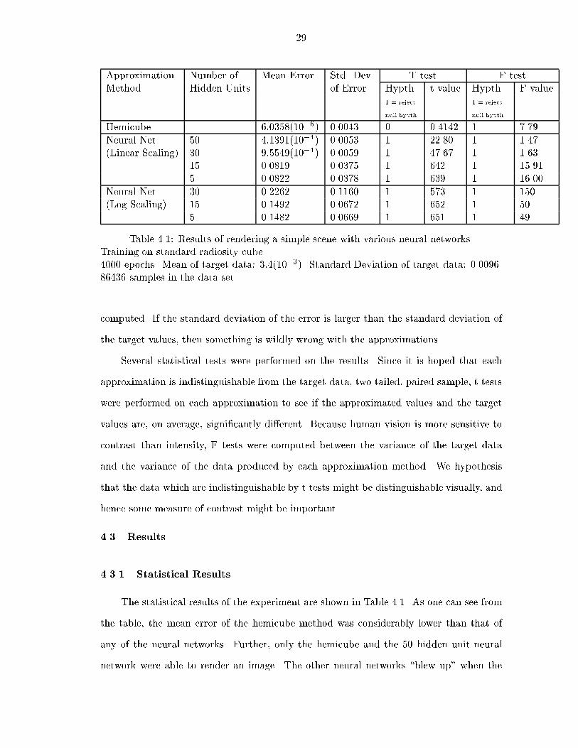
Approximation Number of Mean Error Std. Dev. T test F test
Method Hidden Units of Error Hypth. t value Hypth. F value
1 = reject 1 = reject
null hypth. null hypth.
Hemicube 6:0358(10�6) 0.0043 0 0.4142 1 7.79
Neural Net 50 4:1391(10�4) 0.0053 1 22.80 1 1.47
(Linear Scaling) 30 9:5549(10�4) 0.0059 1 47.67 1 1.63
15 0.0819 0.0375 1 642 1 15.91
5 0.0822 0.0378 1 639 1 16.00
Neural Net 30 0.2262 0.1160 1 573 1 150
(Log Scaling) 15 0.1492 0.0672 1 652 1 50
5 0.1482 0.0669 1 651 1 49
Table 4.1: Results of rendering a simple scene with various neural networks.
Training on standard radiosity cube.
4000 epochs. Mean of target data: 3:4(10�3). Standard Deviation of target data: 0.0096.
86436 samples in the data set.
computed. If the standard deviation of the error is larger than the standard deviation of
the target values, then something is wildly wrong with the approximations.
Several statistical tests were performed on the results. Since it is hoped that each
approximation is indistinguishable from the target data, two tailed, paired sample, t tests
were performed on each approximation to see if the approximated values and the target
values are, on average, signi�cantly di�erent. Because human vision is more sensitive to
contrast than intensity, F tests were computed between the variance of the target data
and the variance of the data produced by each approximation method. We hypothesis
that the data which are indistinguishable by t tests might be distinguishable visually, and
hence some measure of contrast might be important.
4.3 Results
4.3.1 Statistical Results
The statistical results of the experiment are shown in Table 4.1. As one can see from
the table, the mean error of the hemicube method was considerably lower than that of
any of the neural networks. Further, only the hemicube and the 50 hidden unit neural
network were able to render an image. The other neural networks \blew up" when the

30
Rad program tried to render the image: the program exited and core dumped. These
observations can be suggest a practical threshold for the required accuracy of the form
factor calculations. Since each row (or column) of the n by n form factor matrix should
sum to one, the sum of all elements in the form factor matrix should be the number of
rows in the matrix, i.e.
Mean error =
P(FFactorapproximate � FFactoranalytic)
Number of Samples=
P(FFactorapproximate � FFactoranalytic)
(Number of Rows)(Number of Rows)=
Average Row Error
Number of Rows
Hence the mean error over all the form factors multiplied by the number of rows gives the
average error for a given row. If the mean error for the hemicube is multiplied by the 294
rows in the form factor matrix for this scene, the average error per row is about 0.2%.
For the 50 hidden unit, linearly scaled, neural network, this error is 12% and for the 30
hidden unit, linearly scaled, neural network, this error is 28%. Thus, for the Rad program
and for this particular scene, the accuracy of the form factor should be such that the sum
of each row should have 12% error or less in order for the program to run to completion
without problem. More generally, however, this suggests that there is an upper bound on
the acceptable error for the form factor values if a scene is to be successfully rendered.
Comparing the statistical tests for the 50 hidden unit neural network and the hemicube
solution one can see that the t values for the hemicube were more than 50 times lower
than for the neural network while the F values for the hemicube were somewhat higher
than for the neural network. As we shall see later, the hemicube produced a much better
image than the neural network, so the hypothesis that variance is visually more signi�cant
than the overall accuracy of the approximation may be false or at least masked by large
mean error of the neural network.
4.3.2 Visual Results
Plate 1 in Figure 4.3 shows the scene rendered with the analytic method while Plate 2
shows the scene rendered with the hemicube method. Despite the inaccuracies of the

31
Plate 1 (analytic) Plate 2 (hemicube)
Plate 3 (neural network) Plate 4 (red)
Plate 5 (green) Plate 6 (blue)
Figure 4.3: A simple radiosity scene rendered with the analytic, hemicube and neural
network methods.

32
hemicube method, these two images are di�cult to distinguish visibly and the image ren-
dered with the hemicube shows the correct symmetry of red and blue color components
about the vertical center of the image. The hemicube image also shows the correct dim-
ming of all color components with increasing distance from the luminous surface (shown
here as depth into the scene). The scene rendered by the 50 hidden unit neural network as
shown in Plate 3, seems to show the correct fading of color from left to right in the scene.
However, it shows neither the correct dimming with distance from the luminous surface
nor the correct symmetry about the vertical center of the image. Both the hemicube and
the neural network methods took about �ve minutes to render the scene while the analytic
method took several hours.
To further explore the errors in the image rendered by the neural network, three
more images, Plates 4, 5, and 6, were created showing error in the red, green, and blue
components respectively. In the new images, each pixel is the di�erence between the value
rendered by the approximate method and the value rendered by the analytic method. The
images were scaled such that medium gray represents no error, white represents positive
error and black represents negative errors.
It is di�cult to predict how errors in the form factor matrix would a�ect the computa-
tions that follow, but several things might be expected. Since three independent Gaussian
elimination steps are performed to compute the distribution of light for each of the three
color components, one might expect to see symmetric errors in the color computations.
The errors one sees in the green component (Plate 5) do appear to be symmetric, but the
red and blue components (Plates 4 and 6) did not converge to solutions with symmetric
errors. The errors, however, are clearly not randomly distributed across the three error
images, which suggests that inaccuracies are not caused solely by random noise in the
approximation but by systematic inaccuracies in the neural network's approximation of
the form factor integral. In other words, the neural network has not fully learned all the
relevant relationships for form factor calculations. Given that such a simple scene gener-
ated an enormous amount of data to train on, this might suggest that the representation
used to specify the quadrilateral, the x; y and z values of each vertex, may be too vague

33
for the neural network to learn the correct relationships between patches. It is possible
that with even more training data a better approximation could be achieved. However, if
the additional training data introduced more geometrical relationships between patches,
this e�ect could be diluted.

Chapter 5
CONCLUSION
We conclude this report with some observations about the experiments and the im-
plementation of tools used in the experiments. Most important of these observations are
the issues of visibility and representation. Directions for future work are then suggested.
5.1 Visibility
Our statement of the form factor in Equation 2.5 was
Fij =1
Ai
Zx2Pi
Zy2Pj
cos � cos �0
�r2V (x; y)dydx;
which contained the innocuous term V (x; y) where
V (x; y) =
(1; if x and y are mutually visible;
0; otherwise.
In actual implementations, the V (x; y) term can be more problematic than the rest of the
integral.
Several of the most popular form factor approximation methods inherently take visi-
bility into account. The hemicube, for example, casts a ray through each window in the
hemicube and �nds the closest patch that the ray intersects. In this manner, the visible
portion of all patches in the scene (within the limits of the hemicube resolution) are pro-
jected onto the surface of the hemicube. Another popular method, Monte Carlo sampling,
selects a pair of patches and then casts rays between randomly selected beginning and
ending points on the patches. If the cast rays are occluded by other objects, then they
don't contribute to the estimation of the integral and in this manner the V (x; y) term is
accounted for.

35
The naive implementation of the neural network approximation used in this report
simply casts a ray from the center of one patch to the center of another patch to determine
visibility. If the contributing patch is, say, 40% occluded but the ray cast for the visibility
test is not, then the estimate of the form factor will be seriously in error. One solution to
this problem is simply to mesh the scene with smaller patches. However, increasing the
n2 pairs of form factor computations to be done is undesirable. Another solution would
be to cast multiple rays to test visibility for each pair of patches. If either all or none of
the rays are obstructed, then either the full form factor is calculated or it is zero. If a
portion of the rays are obstructed, the patches could be adaptively subdivided until they
were small enough for an \all or nothing" estimation of the form factor.
A novel solution to the visibility problem would be to use the hemicube method to
locate the closest patch and then use the neural network to compute the delta form factor
between the base patch and each window in the hemicube. With a properly implemented
neural network, this could increase the accuracy of the hemicube method, although it
would not address the aliasing problem inherent in the hemicube method nor would it
be able to take advantage in the pre-computation used in the straightforward hemicube
method.
5.2 Representation of the Patches
The representation of the quadrilaterals used in this report, the x; y and z values of
each vertex in the two quadrilaterals, was chosen for two reasons. First, this representation
is easy to extract from routines within the Rad program. Second, these are the required
inputs for the analytic form factor library routines, so they had to be computed anyway.
There is no indication that this representation is optimal. For example, for two patches
there are four ways to start the clockwise listing of vertices. This gives sixteen ways to
list the vertices that are input into the neural network yet each of the ways gives the same
form factor. This redundancy suggests a more concise representation for the patches could
exist.
An interesting test of the current representation would be to take the data from the
simple scene and train the neural network on the dot product of the patch normals. If

36
the neural network would learn this relationship then one could have more faith that the
representation of the problem used here is appropriate.
5.3 Future Work
Several directions exist for future work. The experiments with data from a simple
scene (Table 4.1) suggests that a threshold has been crossed between a neural network
with 30 hidden units, which cannot render a scene and a neural network with 50 hidden
units, which can render a scene. In order to render scenes with more accuracy, larger
neural networks should be tested with the simple scene data in order to see if accuracy
improves.
The experiments with random data illustrate the desirability of an approximation
that produces errors that are proportional to the target value. Although the experiments
which trained the neural network on the logarithm of the target value have produced
results as good as the networks trained on linearly scaled data, this idea should be further
explored in order to reduce the demands on accuracy needed by the neural network.
A more fruitful direction, however, might be to more directly model the integral
sampling one �nds in numerical integration and in Monte Carlo integration. This could
be done by breaking the problem of solving the integral into sampling the two patches
with one layer of a multi-layer network and then computing the contribution to the overall
integral with another layer in the network. The �rst hidden layer of the network might
be trained to have each node in the hidden layer sample a subsection of the of each of the
two patches represented in the input vector. After this layer was trained and hard-coded
into the network, a second hidden layer could be trained to compute the kernel of the
form factor integral for each of the sub-patch pairs found in the previous layer. The ouput
unit would then simply sum up the integral. The total amount of training required of the
neural network might be much reduced by specifying more speci�c subtasks and solving
them independently.

REFERENCES
[Chen 90] Shenchang Eric Chen, Incremental Radiosity: An Extension of Progressive
Radiosity to an Interactive Image Synthesis System, Computer Graphics, Vol-
ume 24, Number 4, August 1990.
[Cohen 85] Michael F. Cohen and Donald P. Greenburg, The Hemi-Cube: A Radiosity
Solution For Complex Environments, SIGGRAPH 85, ACM, 1985.
[Cohen 92] Michael F. Cohen et al., Course Notes 11: Radiosity, SIGGRAPH 92, ACM,
1992.
[Cohen 93] Michael F. Cohen and John R. Wallace, Radiosity and Realistic Image Syn-
thesis, Acedemic Press, 1993.
[Hass 95] Mohamad H. Hassoun, Fundamentals of Arti�cial Neural Networks, MIT
Press, 1995.
[Patt 92] Sumant Pattanaik, Rad code is available by ftp from: wuarchive.wustl.edu in
the /graphics/graphics/radiosity/Rad directory.
[Schro 93] Peter Schr�oder and Pat Hanrahan, On the Form Factor between Two Poly-
gons, SIGGRAPH 93, ACM 1993. Form factor library code is available from:
[Sill 94] Francois X. Sillion and Claude Peuch, Radiosity & Global Illumination, Mor-
gan Kaufman Publishers, 1994
[Sparr 78] E. M. Sparrow and R. D. Cess, Radiation Heat Transfer, Hemisphere Publish-
ing, 1978.