JOURNAL OF MULTIVARIATE ANALYSIS 27, 375-391 (1988)

inference in a Model with at Most One Slope-Change Point

B. Q. MIAO

University of Pittsburgh

Communicated by the Editors

In this paper the problem of slope-change point in linear regression model is discussed with the help of the theory of Gaussian process. The distribution of the estimators of the change point proposed in this paper can be approximated by the first type of extremal distribution. Based on this fact, the detection and interval estimation of a change-point in various situations are discussed. 0 1988 Academic

Press. Inc.

1. INTRODUCTION

Consider the model

x(t) =f(t) + Et, o<t<1,

where f(t) is a nonrandom function with the form

P+Pl(~-kl), f(r)={p+p2(f-lo),

o<t<to to<t< 1.

(1.1)

(1.2)

t, is called the slope change point (off(t), or the model (1.1 )), E, is the ran- dom error of the model, while p, PI, &, and t, are unknown parameters.

For given integer n we take observations of x(t) at t = i/n, i = 1, . . . . n. For simplicity of writing, x(i/n) and e(i/n) will be abbreviated to xi and ei, respectively.

Received March 25, 1988 AMS 1980 subject classifications: Primary 62MO9; Secondary 62E20. Key words and phrases: Asymptotic distribution, change point, detection, Gaussian

process, interval estimate. * Research sponsored by the Air Force Office of Scientific Research under Contract

F49620-58-C-0008. The U.S. Government’s right to retain a nonexclusive royalty-free license in and to the copyright covering this paper, for governmental purposes, is acknowledged.

375 0047-259X/88 $3.00

Copyright 0 1988 by Academic Press, Inc. All rights of reproduction in any form reserved.

376 B. Q. MIA0

The problem of making statistical inference in this model is important in practical applications and of much theoretical interest. Many authors have contributed to it. To name a few among others, Hudson [6], Hinkley [4,5], Feder [3], Krishnaiah and Miao [lo], and Csorgo and Horvath [2].

In this paper we shall propose a method of dealing with this problem. Our method possesses a desirable feature in that the asymptotic dis- tribution of the proposed statistic is very simple, which allows us to derive simple procedures for various inference problems in this model. The basic idea of the method is motivated by recent works of Yin [12] and Chen [l].

In Section 2 we treat the case where si, . . . . E, are normal with zero mean and known variance r?. In Section 3 we consider the normal case with unknown a*. Section 4 considers the nonnormal case. Finally, in Section 5 we discuss the estimation of the slope change /?i - p2 under some mild conditions.

2. NORMAL ERROR WITH KNOWN VARIANCE

In this section we suppose that si, . . . . E, are i.i.d. with mean zero and known variance u*. Our method is based on the following theorem:

THEOREM 1. Suppose that

x,=a+kp+Ek, k = 1, . . . . n, n (2.1)

where Ed, . . . . E, are i.i.d., E~ - N(0, a*). Let m = m, be a positive integer such that

n 9 m $ n213 log2j3 n. (2.2)

Here and in the sequel, u, >> v, > 0 means lim, _ m(~,/v,) = co. Set

Y,=- l r(xk-h+l+ 26

... +Xk-3m)-(Xk-3m+1 + ... +xk-zm)

-CL*??I+, + ... +x,-,)+(Xk-m+,+ ... +xk)],

k = 4m, 4m + 1, . . . . n, (2.3)

rn=4myn IYklY . .

SLOPE-CHANGE POINT 377

and

x x+2log L-5 +5loglog c-5 -$ogrc ( ( 5n ) ’ ( 5n ) ’ ). (2.4)

Then

J\; P($!<A,(x))=erp( -2epx}, -co<<<<. (2.5)

Proof: Construct a standard Brownian Motion { W(t) : t 2 0}, such that

W(g)=&(x,+ . ..+x.-ka-vj?)/c, k=4m,...,n.

(2.6)

Define a Gaussian process Z(f) by

W(t+5)-2W r+‘5 +2W t+: -W(t) ( 4) ( 4) 13 t>O. (2.7)

It is easy to see that

k = 4m, . . . . n,

and the covariance function P(T) of Z(t) is

Set

(2.8)

(2.9)

378 B. Q. MIA0

Similarly to Chen [ 1 ] it can be shown that

lim rl,s= 0, a.s. ” + P

(2.10)

For the Gaussian process Z(r) with covariance function p(r), the conditions of the theorem of Qualls and Watanable [ 1 l] are satisfied, and we get

lim P(rn <A,(x)) = exp{ -2e-“}. n-cc

(2.11)

Since A,(X) is linear in x, for n large we have

P(& < A,(x- lAxI 1) - P(q, 2 I4/JGG)

6 P(5,la 6 47(x))

< P(fn < A,(x + IhI)) + P(rt, 2 I~xll$G). (2.12)

From (2.10) to (2.12), letting n + co, then Ax + 0, we obtain (2.5). This theorem suggests a way to test the null hypothesis that no change

points exists, i.e.,

H,: f?~j?*-/?*=O. (2.13)

For this purpose, we have only to solve the equation exp( -2e-“) = 1 - a for a chosen level CI E (0, 1). The solution is

x(a) = -log( - $ log( 1 - a)).

Set

&!!Ll n’

C”(& 4 = AAX(~ (2.14)

The null hypothesis (2.13) is rejected when and only when

5, > ez(a, 4. (2.15)

From Theorem 1 it is seen that this test has an asymptotic level c1 as the sample size n tends to infinity.

We can give an approximate power /I, = /?&?r, /&, a) of this test. Let r be the integer such that

r+l r<t<-. n n

SLOPE-CHANGE POINT

Then

379

>@ ( ~lf12-BIl-Cn(r.4 , ) (2.16)

where

@(x) = j.r -&e-‘2J2d~.

Next consider the interval estimate of the slope change point to. The existence of t, may be a fact known in advance, but usually it is evidenced by the rejection of the null hypothesis.

RULE. Find an integer k such that 1 Y,l = C;,. Take [(k - 4m)/n, k/n] as the confidence interval of t,.

The length of this interval is 4m/n. Hence, the smaller the value of m, the more accurate is the estimate. m cannot be taken too small, for from (2.16) it can be seen that the risk of false acceptance of the hypothesis (2.13) will increase. We can give an approximate value of the confidence coefficient y of this rule:

y=P k-4m k -<Q(Jd-

n n

2P({ sup k$[r,r+4m]

IY~l~~C,(a,d)}~{lY,+2ml>aCn(a,d)}).

Set

A= { SUP ~~/ct~~~,(~,d)}, 4m<k<r

B={ sup 1 yki < ‘Jcn(K d)}, r+4m<kbn

B,= { sup 1 yki < o’%(% d)}, r+6m<kbn

and

683/27/2-S

C= {IYr+2,1 >~C,(a, 4).

380 B. Q. MIA0

Notice that the event B, is independent of both A and C, and Bc B,, we have

y>P((AuB)C)>P(C)-(P(B,)-P(B))-P(A)P(&),

where D denotes the complementary event of D. Again, using Theorem 1, we get

y>@

(

m3’2 lB2-P1l -c (a

2na n ’ d)

1

- (exp{ -2eP”3(“)} -exp{ -&-‘2(“)})

-(I -exp{ -2eP”l(“)))(l -exp{ -2e--y3ca)}), (2.17)

where

x,=x,(a)=c”(a,d)(210g(~-5))“2

-(210g(-&5)+~loglog(-&5)-~log~), (2.18)

x2=X*(a)=C.(.,d)(210g(~-5))1’2

-(210g(v-5)+floglog(y-+;logn), (2.19)

and

x3=x3(CL)=C,(a,d) I”

- 210g ( (

W-r) 75 -&--- .

1

+$oglog 7- (

5(n - r) 7.5)-;10,.). (2.20)

Since

PC sup I Y/J < GC.(c(, 4) a P( sup I Ykl G OC,(& 4) k4 [r.r+4ml 4m<k<n

%:-CL (2.21)

We get

Y>@ ( m3’*lP2-PII

2no - C,(a, d) - a.

> (2.22)

SLOPE-CHANGE POINT 381

By the above inequalities, we see that y increases with (2no)- *m3” Ifi2 - /Ii/. But the length of the confidence interval is 4m/n. So in the choice of m we must strike a balance between these two considerations. Usually the slope-change point is of practical importance only when IB2- PII is reasonably large as coompared with 6, say I/I2 - /?,I/20 > M, where A4 is a constant decided by practical considerations.

In practical applications we often have to give an answer to the following important question: How can we choose suitable integers m and n so that the confidence interval of t, formed above has a length not greater than do and confidence coefficient not smaller than 1 -cl,? For this purpose, take IX= a,/2 in (2.22). Solve the equations

do = 4m/n; (2.23)

we obtain

m = (4hW2(C,(G& 4) + ~2)~~ n = 4m/do, (2.24)

where uEd2 is the upper percentile (a0/2)-point of N(0, 1). If we know in advance that a < t, < b, for some known constants a, 6,

O<a< b-c 1, then un6r6 bn. From (2.18~(2.20) we can calculate the minimum value I,(Q) of ~,(a,,) and the maximum values Z2(cr,), ?,(a,) of x~(cL,,), x~(cQ,), all under the restriction that an < I < bn. (2.17) suggests that in this case we should choose m as the solution of the equation

Cp (

T&-- CII(ao, do) )

- (exp{ -2e-“3’“0)} -exp( -2eP’2’“0J})

-(l-exp(-2e~“1~“o’})(l-exp(-2e-“3~”0)})=1-a,, (2.25)

and n = 4m/d,, as before. From this we see that if some prior information about t, is available,

then it can be utilized to construct a confidence interval with greater confidence coefficient. Also, the related test will have a smaller critical value.

3. NORMAL ERROR WITH UNKNOWN VARIANCE

When c2 is unknown, we form an estimate, say 6:. Substitute d,, for 0 in (2.15) to perform the test. Following Chen [ 11, we can prove the following theorem.

382 B. Q. MIA0

THEOREM 2. 0’ satisfying

Under the conditions of Theorem 1, if dz is an estimator of

lim ISi - 0*1 log n = 0, in probability. (3.1) n - m

Then

bLrnm P(<,/tin-AJx))=exp{ -2e-“}.

Our problem is to find an estimator satisfying (3.1). We propose to use the MLE of a2 given below in (3.5). It will be shown that this estimator satisfies (3.1).

Suppose x,, . . . . x, are observations from the model (1.1) and (1.2) such that

c11+ ?p, +Eir i=l 9 . . . . nl x; = (3.2)

I*+ 55 p* + Ei, i=n, + 1, . . ..n.

si, . . . . E, are random errors. We assume that the slope-change point to falls into [n,/n, (n, + 1)/n). By (1.2), we have

(3.3)

Let

ZLc = $-i-j $ (C-OXi,

2 zRc=(n-c)(n-c+ l)i=e+,

f (i-c)xi. l-1

THEOREM 3. Suppose that cl, . . . . E, are i.i.d., and cl - N(0, a*). Set

s;,= i (xi-x,,)*+ f (xi-i2,)‘-3c~~-l*)(1;,,-.r,,)* i= 1 i=r+l

3(n-c)(n-c+ 1) n-c-l (E,,. - -f2,1*;

62 nc=$S:c, c = m + 1, . . . . n -m.

(3.4)

(3.5)

SLOPE-CHANGE POINT

Then

m<~~pmIB~,.-a21 lognA0. . .

383

(3.6)

ProoJ Write

ej=(l, . . . . l)ixi, fi=(j- 1, j-2, . . . . l,O)ixi

gj = (1, .-, Al, x jr lJ= (PI, PI> P29 Pd (3.8)

x = (X,) . . . . x,)‘, & = (&I) . ..) E,)‘.

Then

x=F,,,/l+~

and

S;,. = x’(Z- F,.(F,‘F,)- ‘F,‘)x;

where

(3.9)

(3.10)

fil =a,,e,e:.-a,,.f,e:-a,,e,f,: +n~‘adf~, (3.11)

fz=b kc-A,.- 2rgn-r4-c b -b2ce,-.g~-c+n-1b3cgn-cg~-r;

2(2c- 1) 6 12n alc=C(C-I)* a*‘=C(C+ a3c=C(C2

2(2n - 2c + 1) bl’=(tZ-C)(n-C-l)’

6

b*‘=(n-c)(n-c-l)’ 12n

b”=(n-c)(n-r+l)(n-c-lj (3.12)

Without loss of generality, we assume that n > c > n,. Set k z c - n, :

F,.p,,,rFc-F,,. (3.13)

384

We have

(Fe - F,,)‘F,.(F<YyF,’ =

B. Q. MIA0

6k(c-k) %(4c’-9kc+6k2)eL,- c3 f:, c

--$((c”-2kc’+4k’c-2k3)e,,+k(3c-Zk)fk,)

k - 7 ((4~' - 9kc + 6k*) e:, - 6(c - k)fb,)

I --$((2(c-k)‘e:,,-(3c-Zk)/:,,)

4 (c(4c - 3k) e:.- “, -6(c-k)f:.-.,I c

0

1

-~(c(c-k)Ze~-,,+k(3c-2k).f~.~,,) 0 nc

+o i

-{(c(4c-3k)e:.-,,,-6(c-k)f.:-.,) 0 n

0 C

2

-$(c(2c-k)e:-,,- k

(3c-2k)f:.-,,,) -;ekeC J

(3.14)

Set G=F,(FIF,.)-‘F:-F,,(F~,F,~,)-‘F~,=(g,),,,. By a tedious calculation, we can get

GE f: (tr(FC(F,‘FC)-‘F,‘) i=l

+ tr(F,,(~~,F,,)-‘F~,)) E: = 8a2 + 0 0

i , (3.15)

E 1 giisicj 2=~g;04<280a4+0 ; . I I i#j 0

(3.16)

Write y’= p’Fi_,,,(Z- F,(F,‘F,.)-‘F,‘). From (3.14) and (3.3), we get

Var(f.2) = c2 tr(yy’) = a2y’y (3.17)

(3.18)

SLOPE-CHANGE POINT 385

By (3.8), (3.9), and (3.5),

6tc - 8;,,, = -2y’E + E’GE + y’y. (3.19)

Now consider (6:, - 8$, ).

Case 1. b1 #& and k= Ic-n,( an/log*n. We have, by (3.15k(3.18),

P( $,. - s;,, < 0)

= f’( - 27’~ + E’GE < -y’y)

(3.20)

This shows that the minimization point h of (8:,} satisfies

p-n,1 <n/log%

with probability approaching 1 as n -+ co.

Case 2. fi, # j?*, k = Ic - n, ) < n/log* n. It follows that for any u > 0,

< 64 log’ n

u2n2 .y’ya2+~-

410gn 8a2+ 280a4 -ro G&i’

(3.21)

by (3.15)-(3.18).

386 B. Q. MIA0

Now note that x;=r(cf-~~) is a martingale and A,,(AL,A,,) -‘AL, 20. Hence by Marcinkiewicz-Zygmund-Burkholder’s martingale inequality, we have, for any r, S, and u:O<r<6/(1+6), u>O:

un’-’ 6 P (&‘&-no21 >- ( 2 ) (

+ P un’-r

&‘A,,(A~,A,,)-‘A~,&~-- 2 1

f C&JI%l 2+s.-(1+6)(1LT)~n

( un’-’

+ P tr(A,,(AL,A,,)-‘A:,) s’s 22 i

6 C&,JIEI I 2+s”-(a-(l+b)r)+ nT. no2

Cl@, + l)(n-n, + 1) + 0. (3.22)

From Cases 1 and 2, the theorem is true if fll # p2. When /Jr = f12, a similar argument gives

and

J(if,.-cf$l logn-+O

in probability. Thus we complete the proof.

4. NONNORMAL ERROR

When the distribution of random error c(t) is nonnormal, we can use the theory of strong approximation of partial sums of i.i.d. variables by Brownian Motion process to extend Theorem 1 to such cases.

THEOREM 4. Let E,, Ed, . . . be i.i.d. random errors, and the moment generating function of e, exists in some neighborhood or zero, i.e.,

E exp(ts,) < co for 1 tl smafl enough, (4.1)

then the conclusion of Theorem 1 remains valid.

Proof. Put

SLOPE-CHANGE POINT 387

then, by Komlos-Major-Tusnidy [7,8], there exists a Brownian Motion process { W(t), t > 0} such that

bit sup{sup ISk - W(k)l/log n} < co, a.s. (4.2) k<n

Since

yk 1 -=-((s,-2s,_,+2s,_,,-s,-,,), a 2J;;;

we have for 4m < k<n,

yk 1 ---((W(k)-2W(k-m)+2W(k-3m)- W(k-4m)) a 2&

6 - SUP [Sk- W(k)l.

By (4.2), and noticing that log cl,,/& + 0 as n -+ co, we get

(4.3)

lim n-m

---(H’(k)-2W(k-m)

+2W(k-3m)- W(k-4m)) =O, a.s. )I

(4.4)

From Theorem 1, we get

lim P n-m

L(W(k)-2W(k-m)+2W(k-3m)

= exp{ -2ePx}, (4.5)

where A,(x) is defined by (2.5). Thus, (2.6) is also true in view of (4.3)-(4.5). Theorem 4 is proved.

A close inspection of the proof of Theorem 3 convinces us that this theorem is still true under assumption (4.1). Therefore, the method of the previous two sections can be applied.

Further, using a result of Major [9], the following theorem can be established.

THEOREM 5. Let E,,E~,... be i.i.d. random errors with finite (2 + 6)th moment, where 6 > 0, and n D m 9 n 2’(2 + “. Then (2.6) remains true.

Also, the conclusion of Theorem 3 remains valid under the conditions of

388 B. Q. MIA0

Theorem 5. So the previous methods still apply. We note, however, that the requirement on m is more stringent in this case.

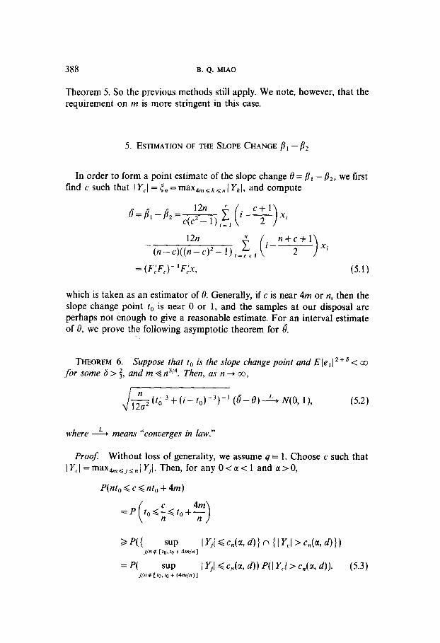
5. ESTIMATION OF THE SLOPE CHANGE j?1-j?2

In order to form a point estimate of the slope change 0 = /I, - /$, we first find c such that ) Y,l = 4, = max,, < k < n 1 Y,J, and compute . .

e^+&-jj*= 12n (’ +! Xi xC c(c’- I),=, )

12n n

-(n-c)((n-c)2-1)i=c+, i- I(

n+c+l 2 > xi

= (F(!F,.) - ‘F,‘x, (5.1)

which is taken as an estimator of 0. Generally, if c is near 4m or n, then the slope change point t, is near 0 or 1, and the samples at our disposal are perhaps not enough to give a reasonable estimate. For an interval estimate of 8, we prove the following asymptotic theorem for 6

THEOREM 6. Suppose that to is the slope change point and E Je,) 2+ * < 00 for some 6 > f, and m G n’14. Then, as n -+ 00,

J &(t;3+(i-t0)-3)-1 (8-0)-LN(O, l), (5.2)

where 4, means “converges in law.”

Proof Without loss of generality, we assume q = 1. Choose c such that IY,.l =maX4mGj.. ) Y,l. Then, for any 0 < a < 1 and a > 0,

P(nt, < c < nto + 4m)

=P t,&t,+2 ( n n >

apt{ sup IYjl~c,(a,d)~n{IY,(>c,(a,d))) ilnC Cbm+4~/nl

= P( sup I Yjl < c,(a, 4) P(l Y,( > c,(a, d)). (5.3) i/n* Ck3.~0+(4mln)l

SLOPE-CHANGE POINT 389

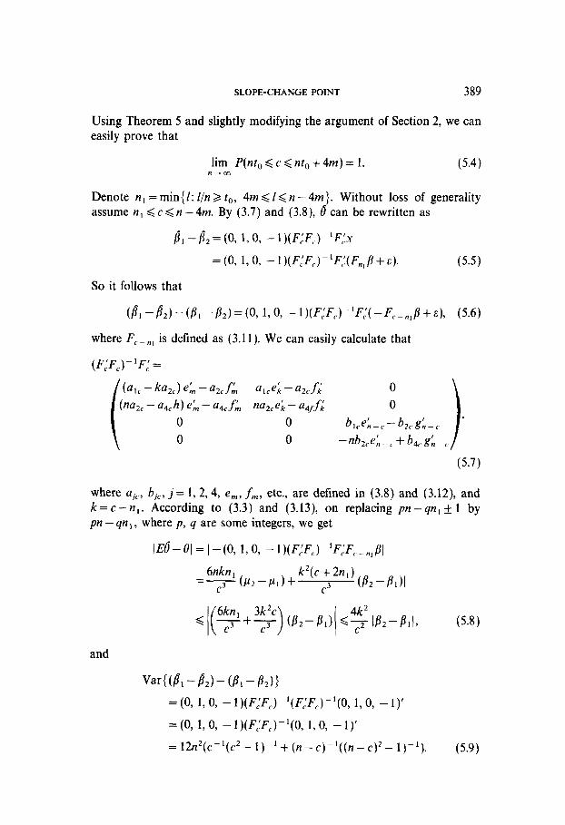
Using Theorem 5 and slightly modifying the argument of Section 2, we can easily prove that

lim P(nt, 6 c < nr, + 4m) = 1. (5.4) n-m

Denote n, =min{l: l/n> t,, 4m < I< n - 4m). Without loss of generality assume n, < c < n - 4m. By (3.7) and (3.8), 6 can be rewritten as

fl, - fl, = (0, l,O, - l)(F,‘F,.)P’F:x

=(O, LO, -l)(F,‘F,.)-‘F,I(F,,B+e). (5.5)

So it follows that

(8,-&)-(/f-C-Bz)=(O, I,% -l)(F,‘F,.)-‘I;,‘(-f;,-.,B+&), (5.6)

where F, _ n, is defined as (3.11). We can easily calculate that

(F,‘F,)-‘F,‘=

(~,c-~~2c~e~-a2cf~ alce~--a,cf,' 0

na2, -~d)d,,--~,fA na+G-a~/f,: 0 0 0 bl.4-.-b2cgL,. ' 0 0 -nb2,eL_, + bdcgAPr 1

(5.7)

where ajC, bjc, j= 1, 2,4, e,, f,, etc., are defined in (3.8) and (3.12), and k= c- n,. According to (3.3) and (3.13), on replacing pn - qn, + 1 by pn - qn 1, where p, q are some integers, we get

(Ed- 8) = ) -(O, 1, 0, - l)(F;F,)-‘F,‘F,.-.,BI

6nkn1 =c3@2-Pd+ k2~c:,2n’+LkPl)I

and

Var{tb, - 19~) - (PI - &)I = (0, 1, 0, - l)(F,‘F,)-‘(F:F,)-‘(0, 1, 0, - 1)’

= (0, 1, 0, - l)(F,‘FJ’(O, l,O, - 1)’

=12n2(c-1(c2-1)~1+(n-c)~1((n-c)2-l)~1). (5.9)

390 B. Q. MIA0

To justify the use of the standard CLT, we note the following three easily verified facts:

1. From the expressions (5.1) and (5.6), we have

Var{(/?,-&)- (8, --/12)}-(*+‘)‘*

x{$, (c(c2_“1))2+’ li-+~2+bElei12+”

+i (

12n 2fd

> I

n+c+l 2+6 i=(+, (n-c)r(n-4*-11 i- 2

Elei(2+6 1

<KEle,lZfs. n*+6(C- 3(2+6)+(3+S)+(,-c)-3(2+6)+(3+6))

,2+a(,-3(2+ar/2+(n_c)-3(2+6)/2)

< 2K(max( c, n - c)) ~ 612 < 2Kc ~ 61-7 < 2Kt - 64, - aI2 + 0, 0 (5.10)

where K is a constant.

2. Since n314 B k, we get

< lim 4kZ)82-PI,.(12n2c~3)-1’2 n-m c2

< lim 2k2

n--tao 3 ton3i*=0’ J

(5.11)

3. It is easy to see that

12n3(c-‘(c~-1)-‘+(n-c)-‘((n-c)*-1)-’)~12(t,3+(1-t,)-3).

(5.12) Theorem 6 is proved.

Notice that i,-- (c- 2m)/n is a consistent estimator of t,. (Of course, only when 13 # 0, hence t, is well defined.) In Section 3 we introduced a consistent estimator 8, of g. Substituting i0 to t, and &‘, for o, we have the following result.

THEOREM 7. Suppose that the conditions of Theorem 6 are satis$ed. We then have

&2(i,-)+(t-iio)-3)-1 1’2{fLHJA N(0, l), (5.13) ”

asn+co.

SLOPE-CHANGE POINT 391

When PI = p2, though t, does not exist, the statistic 2, is still well defined. Since it is not known whether or not (5.13) is true for PI =p2, so (5.13) cannot be used to give a test for the hyperthesis /?, = /$. However, (5.13) can be utilized to form a confidence interval of (/?, -&) if we know fil # p2 a priori, when the null hypothesis (2.13) is rejected.

REFERENCES

[ 1] C&N, X. R. (1987). Testing and Interval Estimation in a Change-Point Model Allowing at Most One Change. Technical Report No. 87-25. Center for Multivariate Analysis, University of Pittsburgh. Sci. Sinica, Ser. A, in press.

[2] Csi%GG, M., AND HORVATH, L. (1986). Nonparametric methods for change-point problems. In Handbook of Sfatistics, Vol. 7. North-Holland, Amsterdam.

[3] FEDER, P. I. (1975). On asymptotic distribution theory in segmented regression problems--Identified case. Ann. Statist. 3, 49-83.

[4] HINKLEY, D. V. (1970). Inference about the change point in a sequence of random variables. Biometrika 51, l-17.

[S] HINKLEY, D. V. (1971). Inference in two-phase regression. J. Amer. Sfatist. Assoc. 66, 736743.

[6] HUDSON, D. J. (1966). Fitting segmented curves whose join points have to be estimated. J. Amer. Statist. Assoc. 61, 1097-1129.

[7] KOML~S, J., MAJOR, P., AND TUSNADY, G. (1975). An approximation of partial sums of independent R.V.‘s, and the sample DF. Part I. Z. Wahrsch. Verw. Gebiete 32, 111-131.

[S] KOML~S, J., MAJOR, P., AND TUSNADY, G. (1976). An approximation of partial sums of independent R.V.‘s and the sample DF. Part II. Z. Wahrsch. Verw. Gebiete 34, 33-58.

[9] MAJOR, P. (1976). The approximation of partial sums of indepdent R.V.‘s Z. Wahrsch. Verw. Gebiete 35, 213-220.

[lo] KRISNAIAH, P. R., AND MIAO, B. Q. (1987). Review about Estimation of Change-Point. Technical Report No. 87-48. Center for Multivariate Analysis, University of Pittsburgh. In Handbook of Statistics. Vol. 7. North-Holland, Amsterdam.

[11] QUALLS, C., AND WATANABE, H. (1972). Asymptotic properties of Gaussian processes. Ann. Math. Statist. 43 580-596.

[ 121 YIN, Y. Q. (1986). Detection of the Number, Locations and Magnitudes of Jumps. Technical Report. University of Arizona.