powering of endoscopic cutting tools for minimally
TRANSCRIPT
Powering of endoscopic cutting tools for
minimally invasive procedures
A Thesis
submitted to the faculty of the
Worcester Polytechnic Institute
as a partial fulfillment of the requirements for the
Degree of Master of Science
in
Mechanical Engineering
By
________________________
Kehui Chen
28 May 2013
Approved:
______________________________
Prof. Cosme Furlong, Major Advisor
__________________________________________________
Prof. Ryszard J. Pryputniewicz, Member, Thesis Committee
____________________________________________
Prof. Maria Chierichetti, Member, Thesis Committee
_________________________________________________________________
Jeffery B. Ryan Jr, Interscope, Inc., Whitinsville, MA, Member, Thesis Committee
________________________________________________
Prof. Simon W. Evans, Graduate Committee Representative

Copyright © 2013
By
NEST – NanoEngineering, Science and Technology
CHSLT – Center for Holographic Studies and Laser micro-mechaTronics
Mechanical Engineering Department
Worcester Polytechnic Institute
Worcester, MA 01609-2280
All rights reserved
i
Abstract
Sample cutting is an important minimally invasive medical procedure. Currently
there are several types of medical devices used to cut a distal biological sample, for
example, a video endoscope and TurboHawk Plaque Excision Systems.
Directional Atherectomy (DA) with the TurboHawk Plaque Excision Systems is a
catheter-based, minimally invasive treatment method for peripheral arterial disease (PAD).
During a procedure, a catheter is directed toward an area of plaque buildup to remove the
plaque from the body, restoring blood flow (Covidien, 2013).
Endoscopy is an important procedure used in the medical field to study and diagnose
different parts of a body without the need to undergo a major surgery. The major
devices are a video endoscope with a flexible or rigid insertion tube and endoscopic
therapy devices. Arrays of the devices, through the instrument channel in the insertion
tube of endoscopes, to perform a variety of functions are offered. The biological sample
cut is one of the important endoscopic therapies.
Both of Directional Atherectomy and endoscopy procedures require a power
transmission from the proximal tip of device to the distal end, where the cutter is located,
for cutting a sample. However, the working length is up to meters, and the diameter of
the devices is in millimeter scale in the minimally invasive surgery. Thus enough power
transmitting to the distal end of the device for the biological sample cutting is crucial.
This research presents the effort toward the investigation of the potential power

ii
mechanisms from the proximal tip to the cutter at the distal end of the device for rapid
rotational cutting motion to improve the cutting efficiency and accuracy.
In this thesis, the potential powering mechanisms including fluid, electrical, and torque
coils are investigated.
Since the transmission power is used for a rotational cutting action, and the cutting
geometry has influence on the cutting power, thus this research also focuses on the
analysis of the cutting geometry for the rotational sample cutting. The Hertz contact
theory and von Mises yield criterion are used to find the influence of tool geometry on
the material removing process, as well as Abaqus, a commercial FEM software, is used
for the finite element analysis. Fiber-reinforced composite structures are the main
characteristic of the representative biological sample, and their mechanical behavior is
strongly influenced by the concentration and structural arrangement of constitute such as
collagen and elastin. Researches show that the biological sample, for example, a soft
biological sample, has hyperelastic properties and behave anisotropically, and there are a
few publications about the plastic properties and cutting mechanics. Thus a linear
elastic and linear plastic material model is defined for the finite element analysis of
material removal. The analytical results and finite element results both show that as
the tool rake angle increases or the tool angle decreases, the magnitude of cutting force
decreases.
A preliminary representative sample cutting experiment was conducted, and standard

iii
cutters with different cutting geometries were tested in order to find the characteristic of
the biological sample cutting and the influence of tool geometry on the required cutting
power. The experiments reveal the same conclusions as the analytical and finite element
results.
Keywords: Abaqus, contact stress, cutting geometry, minimally invasive surgery,
sample cutting, von Mises yield criterion

iv
Acknowledgments
I would like to thank my advisor Professor Cosme Furlong for giving me the
opportunity to do my thesis on such an exciting area of research and for the guidance he
has provided along the way. The project would not have made it as far as it did without
the help of all the members of the Center for Holographic Studies and Laser
micro-Mechatronics. I would like to particularly appreciate Interscope sponsoring me
during this project.
Accolades are also extended to Babak Seyed Aghazadeh, Caoyang Ti, Zhibo Cao,
Ellery Harrington, Ivo Dobrev, Morteza Khaleghi Meybodi, Weina Lu, Peter Hefti,
Xiaoran Chen, and Weiyuan Tie from the CHSLT laboratories for their enduring support
and invaluable assistance.
Finally, I want to thank my dear family for their love and unending support throughout
my tenure. Without them I would not have been able to accomplish anything.

v
Table of contents
Abstract ............................................................................................................................ i
Acknowledgments.......................................................................................................... iv
Table of contents ............................................................................................................. v
List of figures ................................................................................................................. ix
List of tables ................................................................................................................ xvii
Nomenclature ............................................................................................................. xviii
Objectives .................................................................................................................. xxiii
1. Introduction ............................................................................................................. 1
1.1 Directional atherectomy with TurboHawk system ......................................... 1
1.2 Endoscopic sample cutting ............................................................................. 4
1.2.1 Endoscopy and endoscopes..................................................................... 4
1.2.2 Endoscopic devices for sample cutting ................................................... 9
1.2.2.1 Biopsy forceps .................................................................................... 9
1.2.2.2 Aspiration needles and cytology brushes ..........................................11
1.3 Common characteristics and challenges ........................................................11
2. Potential powering mechanisms ........................................................................... 13
2.1 Fluid-compressed air/water ........................................................................... 13
2.2 Electrical ....................................................................................................... 17
2.3 Mechanical mechanism- torque coil ............................................................. 19

vi
3. Mechanics of cutting ............................................................................................. 27
3.1 Introduction ................................................................................................... 27
3.2 Axial symmetrical elastic analysis ................................................................ 29
3.3 Sphere contact flat surface ............................................................................ 30
3.4 Rigid cone contact surface ............................................................................ 35
3.5 Orthogonal cutting ........................................................................................ 39
3.6 Two-dimensional photo-elastic fringe patterns of rigid cones ...................... 42
4. Finite element analysis .......................................................................................... 44
4.1 Introduction ................................................................................................... 44
4.1.1 Introduction of Abaqus ......................................................................... 44
4.2 Chip separation criterion ............................................................................... 45
4.2.1 Finite element approach ........................................................................ 45
4.2.2 Element failure model ........................................................................... 47
4.2.3 Element removal ................................................................................... 48
4.3 Model definition............................................................................................ 50
4.4 Material properties definition ....................................................................... 52
4.4.1 Biological samples structure and mechanical properties ...................... 52
4.4.2 Limitation of modeling biological sample fracture in Abaqus ............. 54
4.4.3 Material properties definition ............................................................... 54
4.5 Definition of mesh ........................................................................................ 57

vii
4.5.1 Definition of mesh element type ........................................................... 57
4.5.2 Definition of mesh element size ........................................................... 58
4.6 Definition of boundary condition .................................................................. 60
4.6.1 Surface contacts .................................................................................... 60
4.6.1.1 Surface contacts in specimen ............................................................ 60
4.6.1.2 Dynamic surface contacts between cutting tool and specimen ........ 61
4.6.2 Node constrain of the specimen ............................................................ 64
4.7 Definition of load condition .......................................................................... 65
4.8 Stability analysis ........................................................................................... 66
4.9 Results and discussions ................................................................................. 67
4.9.1 Fluctuations in the curve ....................................................................... 69
4.9.2 Cutting process regions ......................................................................... 69
4.10 Rake angle analysis ................................................................................... 71
5. Preliminary biological sample cutting experiments .............................................. 74
5.1 Experiment system set up ............................................................................. 74
5.2 Biological sample cutting experiment result................................................. 75
5.3 Biological sample cutting experiments of using different cutting tools ....... 76
6. Conclusions and discussions ................................................................................. 79
6.1 Powering mechanisms .................................................................................. 80
6.2 Cutting tool geometry analytical ................................................................... 83

viii
6.2.1 Cutting tool geometry analytical analysis ............................................. 83
6.2.2 Cutting tool geometry 2D finite element analysis ................................ 84
6.2.3 Preliminary biological sample cutting experiments .............................. 85
7. Future work ........................................................................................................... 87
8. References ............................................................................................................. 88

ix
List of figures
Fig. 1.1. TurboHawk System (Covidien, 2013). ................................................................. 1
Fig. 1.2. (a) A four contoured blades cutter at the distal end of the flexible
drive shaft in TurboHawk System (Covidien, 2013); (b) Sample
removal using the cutter at the distal end of the flexible drive shaft
in TurboHawk System (Covidien, 2013). ........................................................... 2
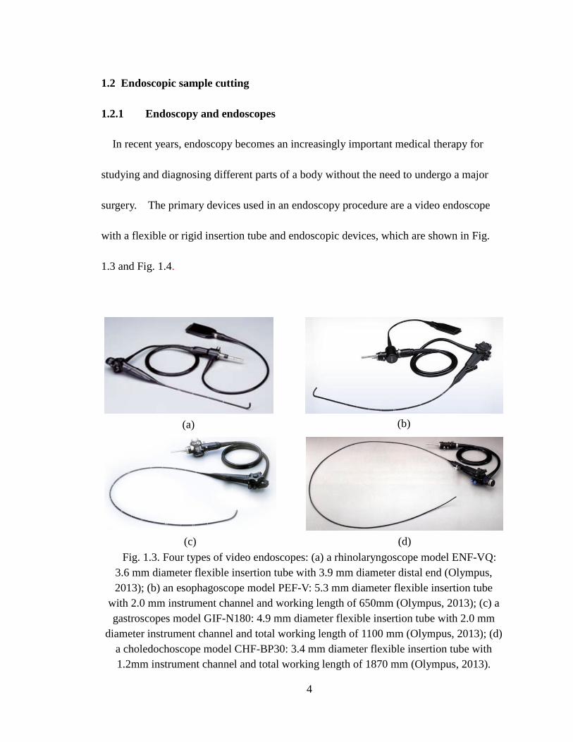
Fig. 1.3. Four types of video endoscopes: (a) a rhinolaryngoscope model
ENF-VQ: 3.6 mm diameter flexible insertion tube with 3.9 mm
diameter distal end (Olympus, 2013); (b) an esophagoscope model
PEF-V: 5.3 mm diameter flexible insertion tube with 2.0 mm
instrument channel and working length of 650mm (Olympus, 2013);
(c) a gastroscopes model GIF-N180: 4.9 mm diameter flexible
insertion tube with 2.0 mm diameter instrument channel and total
working length of 1100 mm (Olympus, 2013); (d) a
choledochoscope model CHF-BP30: 3.4 mm diameter flexible
insertion tube with 1.2mm instrument channel and total working
length of 1870 mm (Olympus, 2013). ................................................................ 4
Fig. 1.4. Endoscopic devices: (a) grasping forceps (Foreign body retrieval,
2013), (b) hemostatic clips (Hemostasis Products, 2013), (c) biopsy
forceps (EndoJaw, 2013), (d) aspiration needle (EZ Shot2, 2013). ................... 5

x
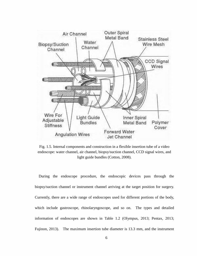
Fig. 1.5. Internal components and construction in a flexible insertion tube of a
video endoscope: water channel, air channel, biopsy/suction
channel, CCD signal wires, and light guide bundles (Cotton, 2008). ................ 6
Fig. 1.6. The distal end of a video endoscope including light guide,
biopsy/suction channel, water nozzle, air nozzle and CCD camera. .................. 7
Fig. 1.7. Biopsy forceps and the working principle of biopsy forceps: (a)
biopsy forceps with a control handle, a flexible tube, and a cutting
tip; (b) biopsy forceps inserted into endoscope instrument channel
and arriving at target area; (c) biopsy forceps approaching to the
target area; (d) biopsy forceps cutting sample; (e) biopsy forceps
collecting sample (EndoJaw, 2013). ................................................................. 10
Fig. 1.8. (a) Aspiration needle; (b) Cytology brushes (Enteroscopy, 2013). .....................11
Fig. 2.1. Fluid flow in a bent tube, the energy losses due to the friction caused
by shear stress along tube walls and the local losses that arises at
tube bends and contractions. ............................................................................ 14
Fig. 2.2. Energy lost due to friction to the total energy along the pipe length. .............. 16
Fig. 2.3. (a) Torque coil schematic drawing (ASAHI INTECC, 2013), and
actual torque coil of 2.210mm outer diameter. ................................................. 19
Fig. 2.4. Torque coil rotation speed measurement system: 1 are DC motor and
DC motor power supplier; 2 is the torque coil within PVC tube; 3 is

xi
LED controller; 4 is function generator; 5 is LED; 6 is CCD
camera;7 is PC. ................................................................................................. 21
Fig. 2.5. Representative images of the distal tip of torque coil rotating at
speed of 400 rpm captured by the camera in time interval of 0.15s.
The capture time period is determined by the strobe light frequency.
When the strobe light frequency is equal to the frequency of torque
coil rotation, the captured images are the same, which is “frozen”. ................ 22
Fig. 2.6. Different rotational speed tests for finding the maximum rotation
speed of sample 1: (a) low rotation speed test, (b) high rotational
speed test. ......................................................................................................... 23
Fig. 2.7. Different rotational speed tests for finding the maximum rotation
speed of sample 2: (a) low rotation speed test, (b) high rotational
speed test. ......................................................................................................... 24
Fig. 2.8. Torque coil failed during the rotation test shown in Fig. 2.4. The
failure occurs at the connection with the motor. .............................................. 25
Fig. 3.1. A deformable plate responds to a normal load applied by a rigid cone:
(a) a normal load is applied, there is elastic deformation in the plate;
(b) if the load is removed, the deformation of plate recovers due to
the elastic deformation; (c) the increment of the load and contact
lead the deformation to increase; (d) the plastic and elastic

xii
deformation occur; if the load is removed, there is some elastic
recovery; (e) the increment of the load and contact lead to the
plastic deformation increase and fracture occur; (f) there is fracture
occurring on the plate. ...................................................................................... 28
Fig. 3.2. Contour of equal maximum shear stress for spherical contact
calculated for Poisson's ratio 3.0v . Distances r and z normalized
to the contact radius a and stresses expressed in terms of mean
contact pressure. ............................................................................................... 32
Fig. 3.3. Contour of equal von Mises stress for spherical contact calculated
for Poisson's ratio 3.0v . Distances r and z normalized to the
contact radius a and stresses expressed in terms of mean contact
pressure. ............................................................................................................ 33
Fig. 3.4. The ratio of stress distribution to contact pressure along z-axis below
the contact area of the contact between a sphere and a flat surface
for Poisson’s ratio 3.0v . .............................................................................. 34
Fig. 3.5. Conical contact stress distribution along z-axis for cone ................................... 37
Fig. 3.6. Conical contact von Misese stress distribution of von Mises along
z-axis for cone semi-angle of 15, 30, 45and 60, respectively. ................... 37
Fig. 3.7. Slip-line theory in two dimensions by Hill et al., 1947,
(Fischer-Cripps, 2007). ..................................................................................... 38

xiii
Fig. 3.8. Illustration of the force components and angles in orthogonal cutting:
Fc is the cutting force along the tool travel direction; Ft is the
thrust force normal to the travel direction; F is the friction force
that resists the movement of the chip while N is the normal force; R
is the resultant force. ........................................................................................ 40
Fig. 3.9. Photoelasticity system developed at CHLST labs. ............................................. 42
Fig. 3.10. Photoelastic stress fringe patterns of rigid cone: a pure normal load
is applied by a rigid cone with semi-angle of 30. As the load is
increased, the number of fringes representing the stress distribution
within the plate increases, as shown from (a) to (i).......................................... 43
Fig. 4.1. Element failure model uses the splitting line for cutting process
analysis in Abaqus. (A) is the specimen, and (B) is the cutting
tool. In the specimen, (1) is the uncut chip; (2) is the splitting line;
(3) is the base. In Abaqus, the element failure criterion is defined
on the splitting line, thus the element of the splitting line is
removed when the deformation or stress of elements in the splitting
line meets the failure criterion in order to separate the uncut chip
from the specimen. ........................................................................................... 49
Fig. 4.2. Cutting tool geometry: (a) the cutting tool; (b) the uncut chip; (c) the
splitting line. ..................................................................................................... 51

xiv
Fig. 4.3. Load-elongation curve for a ligamentum flavum tested in tension to
failure (Nachemson and Evans, 1968). ............................................................ 53
Fig. 4.4. Definition of material plastic stress-strain in Abaqus. Abaqus splits
the material elastic and plastic stress strain curve into two separate
parts including elastic stress-strain curve and plastic stress-strain
curve. The plastic strain starts from 0. .......................................................... 55
Fig. 4.5. Finite elements: (a) the triangle element; (b) the quadrilateral
element. ............................................................................................................ 57
Fig. 4.6. Integration elements: (a) full-integration element; (b)
reduced-integration element. ............................................................................ 58
Fig. 4.7. Finite element results of three meshing sizes. ................................................. 60
Fig. 4.8. Illustration of dynamic contact between tool and specimen............................... 62
Fig. 4.9. Definition of boundary condition of the specimen in Abaqus: the
constraint of all degree of freedom of the nodes at the specimen’s
edges makes sure the specimen not to move during the cutting
process. ............................................................................................................. 64
Fig. 4.10. Definition of load condition in Abaqus. Reference point is used to
apply the load in Abaqus. In the rotational cutting process, the
rotation speed is applied to the RP, and the tool rotates taking the
RP as the rotation center at the applied rotation speed. .................................... 65

xv
Fig. 4.11. Finite element result of the magnitude of the cutting force when the
cutting tool rotation speed is 1900 rpm, and the uncut chip
thickness is 0.1 mm. Point O represents the cutting tool contacts
the specimen. From point O to point A, as the increment of the
contact between the cutting tool and the specimen, the magnitude
of stress on the contact surface is increasing due to elastic
deformation. Point A represents the contact force is up to the
ultimate stress. From point A to point B the force is up to material
ultimate stress, the material is removed continuously till all the
material is removed. From point B to point C, since the material
is removed, and there is little or no contact between the cutting toll
and the specimen, the magnitude of the cutting force decreases...................... 68
Fig. 4.12. Material deformation and fracture during the cutting process: (a)
the cutting tool contacts the specimen, and there is elastic and
plastic deformation in the specimen; (b) as the increment of
contacts between the cutting tool and the material, the specimen
starts to fracture; (c) the chip is almost separated from the specimen;
(d) the chip is totally separated from the specimen. ......................................... 70
Fig. 4.13. Comparison of magnitude of cutting force of the cutting tools with
rake angle 10, 20, and 30 when the cutting rotation speed is

xvi
1900 rpm, and the uncut chip thickness is 0.1 mm. ......................................... 71
Fig. 5.1. Scheme of preliminary biological sample cutting experiment using
torque coil as the power transmission for the rotational cutting
actions. .............................................................................................................. 74
Fig. 5.2. Raw experimental data from preliminary biological sample cutting
experiment at rotation speed 1000 rpm. “Event” represents the
instant when the tool contacts the sample. ....................................................... 75
Fig. 5.3. Cutting tools used in experiments: (a) Tool A with a flat cutting edge,
(b) Tool B with a teeth cutting edge. The outer diameter of both
tools is 2.6 mm. The length of the cutting edge is 4.0mm, and the
width of cutting window is ............................................................................... 76
Fig. 5.4. Cross section of the cutting edge of the tested tools: (a) Tool A; (b)
Tool B. The cutting tool geometries are shown in Table 5.1. ........................ 77
Fig. 5.5. Experimental results of the cutting torque for one revolution
obtained by tested tools at rotation speed of 3000 rpm. “Event”
represents the instant when the tool contacts the sample. ................................ 78

xvii
List of tables
Table 1.1. Geometry information of the TurboHawk System (Covidien, 2013). ............... 3
Table 1.2. Types of endoscopes. ......................................................................................... 8
Table 2.1. Performance data of the electromagnetic micro motor (Gao et al.,
1998). ................................................................................................................ 18
Table 2.2. Major dimensions of the torque coil samples (ASAHI INTECC,
2013). ................................................................................................................ 20
Table 4.1. Comparison of assumed specimen and cutting tool material
properties. ........................................................................................................ 56
Table 4.2. Number of elements in three meshing models. ................................................ 59
Table 4.3. Stable time increment of the models with different element sizes in
Abaqus. ............................................................................................................. 67
Table 4.4. Comparison of analytical and FEM results of the magnitude of ..................... 72
Table 5.1. Cutting tools geometries of tested tools. .......................................................... 77
Table 6.1. Comparison of the potential power mechanisms. ............................................ 82

xviii
Nomenclature
DA Directional Atherectomy
PAD Peripheral arterial disease
frictionh Head loss in a pipe flow
localh Energy loss due to channel bends in a pipe flow
1 , 2 Fluid density at location 1 and location 2 in a pipe flow,
respectively
1z , 2z Distances between location 1 and location 2 to the ground,
respectively
1p , 2p Fluid static pressures at location 1 and location 2 in a pipe
flow, respectively
f Channel friction factor
D Pipe inner diameter
Q Fluid flow rate in pipe
Re Reynolds number
Fluid kinematic viscosity
0E Induced voltage in the armature in a motor
Z Total number of conductors in armature of a motor
Φ Magnetic flux per pole in a motor

xix
N Rotation speed of a motor
B Magnetic material’s magnetic induction
l Length of a rotor in a motor
r Radius of a rotor in a motor
sE Source voltage of a motor
aR Armature resistance of a motor
Electrical resistivity of copper in a motor
L Total length of copper wire in a motor
LED Light-emitting diode
CCD Charged coupled device
PVC Polyvinyl chloride
Hoop stress in cylindrical polar coordinates
r Radial stress in cylindrical polar coordinates
z Axial stress in cylindrical polar coordinates
mp Contact mean pressure in sphere contacts plate problem
a Contact radius in contact problem
0p Maximum contact pressure in sphere contacts plate problem
E Young’s modulus
Possion’s ratio in contact problem

xx
projectA Projected contact area in contact problem
V Velocity of the material in orthogonal cutting model
0 Shear angle in orthogonal cutting model
0 Rake angle in orthogonal cutting model
Friction angle in orthogonal cutting model
Friction coefficient between cutting tool and material in
orthogonal cutting model
Cutting tool angle in orthogonal cutting model
Clearance angle in orthogonal cutting model
f Vector of displacement at any point of the element in FEM
N Matrix of shape functions in FEM
e Vector of nodal displacements at any point of the element in
FEM
Vector of strain at any point of the element in FEM
B Strain-displacement matrix in FEM
Vector of stress at any point of the element in FEM
D Elastic matrix related to the material elastic properties in FEM
ek Element stiffness matrix in FEM
k Structure stiffness matrix in FEM

xxi
F Force vector in FEM
Nodal displacement vector of all elements in FEM
Damage parameter in element failure model in Abaqus
pl Initial value of the equivalent plastic strain in element failure
model in Abaqus
pl An increment of the equivalent plastic strain in element failure
model in Abaqus
pl
f Strain at failure in element failure model in Abaqus
A A point on the deforming mesh of specimen in element failure
model in Abaqus
AX The current coordinate of point A on the deforming mesh of
specimen in element failure model in Abaqus
C A point in the cutting tool in element failure model in Abaqus
CX The current coordinate of point C on the deforming mesh of
specimen in element failure model in Abaqus
'A Closest point on the surface of the cutting tool to point A
n Normal vector from point 'A to point A
r Vector from point C to point 'A
h Distance between point A and point 'A

xxii
c Clearance below which contact occurs
t Tangents to the surface at point 'A
S Measure distance along t to the surface at point 'A
‘Slip’ of point 'A
h Velocity term
h Acceleration terms
RP Reference point
t Stable time increment in FEM
max Highest frequency of the system in FEM
eL Element length in FEM
dc Wave speed of the material in FEM
CPS4R A 4-node bilinear plane stress quadrilateral, reduced
integration, hourglass control element type

xxiii
Objectives
Sample cutting is an important minimally invasive medical procedure. Since the
working length of the current devices, for example, the video endoscope and the
TurboHawk system, is up to meters, and the diameter is in millimeter-scale, achieving
enough cutting power for rotational cutting at the distal end of the devices is a challenge.
Our research presents the effort toward the investigation of the feasibility of potential
power mechanisms from the proximal tip to the cutter at the distal end of the devices for
a rotational cutting motion to improve the cutting efficiency and accuracy. In this thesis,
the potential powering mechanisms including fluid, electrical, and mechanical
mechanisms are investigated.
In addition, the cutting geometries are analyzed due to the influence on the rotational
cutting performance such as cutting power.

1
1. Introduction
Sample cutting is an important minimally invasive procedure. In this Chapter, the
current devices are introduced. In addition, current common characteristic and
challenge of the distal biological sample cutting are presented for aid in determining the
need of the investigation of the powering mechanisms for the rotational cutting at the
distal end of the devices for rapid and accurate sample cutting to perform minimally
invasive surgical procedures.
1.1 Directional atherectomy with TurboHawk system
The TurboHawk System is a directional atherectomy platform to safely treat peripheral
arterial disease (PAD) above and below the knee (Covidien, 2013). The TurboHawk
system contains a flexible drive shaft, a control handle, and a cutter at the distal end of
the flexible drive shaft, which is shown in Fig. 1.1.
Fig. 1.1. TurboHawk System (Covidien, 2013).

2
The cutter at the distal end of the flexible drive shaft, as shown in Fig. 1.2 (a), is used
to cut the sample. An access device, such as a guidewire or a sheath, is placed in the
target vessel. Then the TurboHawk device approaches the plaque burden in vessel along
the access device. When the cutter contacts the sample, it starts to rotate and moves
forward by the control of the proximal tip of the flexible shaft, which is shown in Fig. 1.2
(b).
(a)
(b)
Fig. 1.2. (a) A four contoured blades cutter at the distal end of the
flexible drive shaft in TurboHawk System (Covidien, 2013); (b) Sample
removal using the cutter at the distal end of the flexible drive shaft in
TurboHawk System (Covidien, 2013).

3
The rotational cutting action or cutting power is transmitted from the proximal end of the
flexible drive shaft to the cutter at the distal end of the flexible shaft. The working
length of the TurboHawk system is up to meter, the diameter is in millimeter scale, which
are shown in Table 1.1.
Table 1.1. Geometry information of the TurboHawk System (Covidien, 2013).
Catalog
Number
Vessel
Diameter
(mm)
Crossing
Profile
(mm)
Working
Length
(mm)
Effective
Length
(mm)
Max. Cut
Length
(mm)
LA
RG
E V
ES
SE
L
THS-LS-C
3.5-7.0 2.7
1100
1040
50
THS-LX-C 1300 75
TH-LS-M 1100 50
TH-LX-M 1130 75
SM
AL
VE
SS
EL
THS-SX-C
2.0-4.0 2.2
1350
1290
40
THS-SS-C 1330 20
THS-SS-CL 1490 1450 20
P4028 1.5-2.0 1.9 1350 1320 10
4
1.2 Endoscopic sample cutting
1.2.1 Endoscopy and endoscopes
In recent years, endoscopy becomes an increasingly important medical therapy for
studying and diagnosing different parts of a body without the need to undergo a major
surgery. The primary devices used in an endoscopy procedure are a video endoscope
with a flexible or rigid insertion tube and endoscopic devices, which are shown in Fig.
1.3 and Fig. 1.4.
Fig. 1.3. Four types of video endoscopes: (a) a rhinolaryngoscope model ENF-VQ:
3.6 mm diameter flexible insertion tube with 3.9 mm diameter distal end (Olympus,
2013); (b) an esophagoscope model PEF-V: 5.3 mm diameter flexible insertion tube
with 2.0 mm instrument channel and working length of 650mm (Olympus, 2013); (c) a
gastroscopes model GIF-N180: 4.9 mm diameter flexible insertion tube with 2.0 mm
diameter instrument channel and total working length of 1100 mm (Olympus, 2013); (d)
a choledochoscope model CHF-BP30: 3.4 mm diameter flexible insertion tube with
1.2mm instrument channel and total working length of 1870 mm (Olympus, 2013).
(d) (c)
(a) (b)

5
An endoscope is a major diagnostic, therapeutic, and screening tool used to view inside
the body by inserting the flexible or rigid insertion tube into a natural or created aperture
in the body without the need to make a major surgical incision. The crucial component
of endoscopes is the insertion tube, which may be rigid or flexible. The important
internal components in insertion tube include the water channel, air channel, light guide,
objective lens or eyepiece, and biopsy or instrument channel as shown in Fig. 1.5.
Fig. 1.4. Endoscopic devices: (a) grasping forceps (Foreign body
retrieval, 2013), (b) hemostatic clips (Hemostasis Products, 2013), (c)
biopsy forceps (EndoJaw, 2013), (d) aspiration needle (EZ Shot2, 2013).
(a) (b)
(c) (d)
6
During the endoscope procedure, the endoscopic devices pass through the
biopsy/suction channel or instrument channel arriving at the target position for surgery.
Currently, there are a wide range of endoscopes used for different portions of the body,
which include gastroscope, rhinolaryngoscope, and so on. The types and detailed
information of endoscopes are shown in Table 1.2 (Olympus, 2013; Pentax, 2013;
Fujinon, 2013). The maximum insertion tube diameter is 13.3 mm, and the instrument
Fig. 1.5. Internal components and construction in a flexible insertion tube of a video
endoscope: water channel, air channel, biopsy/suction channel, CCD signal wires, and
light guide bundles (Cotton, 2008).

7
channel diameter varies from 0.75 mm to 6.0 mm. The working length is from 250mm
to 2180 mm. Figure 1.6 shows a distal end of a video endoscope with instrument
channel.
CCD Camera Water
nozzle
Biopsy/Suction
channel
Light guide
Air nozzle
Fig. 1.6. The distal end of a video endoscope including light guide,
biopsy/suction channel, water nozzle, air nozzle and CCD camera.

8
Table 1.2. Types of endoscopes.
Name Application
tissue
Field of
View
(degree)
Insertion
tube
diameter
(mm)
Instrument
channel
diameter
(mm)
Working
length
(mm)
Tip
Deflection
(degree)
Rhinolaryngoscop
e
Nose and
throat
75/85/90 1.8-4.9 --/2 270-635 Up/Down
130
Larynogoscope Throat 90 3.0-5.2 1.2-3.0 600 Up/Down
120
Gastroscope Stomach 120/140 5.1-12.8 2.0-6.0 925-1100 Up 210
Down 90
Right 100
Left 100
Bronchoscope Bronchial
tubes
80 /120 3.8-7.0 1.2-3.6 550-840 Up
120-180
Down
90-130
Choledochoscope Bile duct 90/125
air
83water
2.8-4.9 0.75-2.2 900-1870 Up 160
Down 130
Duodenoscope Designed
for
ERCP
A side
view:
90/100
7.4-12.6 2.0-4.8 250-1030 Up 120
Down90
Left 90
Right 110
Enteroscope Duodenum 140 5.0-13.2 1.0-3.5 800-2180 Up/Down
180
Right/Left
160
Sigmoidoscope Rectum
and
sigmoid
colon
120/140 12.2-13.3 3.2-4.2 630-790 Up/Down
180
Right/Left
160
Colonoscope Colon 140/170 12.8-13.2 3.2-4.2 700-2180 Up/Down
180
Right/Left
160

9
1.2.2 Endoscopic devices for sample cutting
The biopsy forceps or aspiration needles are used for sample cutting, which pass
through the instrument channel of endoscopes. The transmission length of the sample
cutting action from the proximal tip of the endoscopic device to the removal tools at the
distal end is up to meters, and the crossing profile is in millimeter scale.
1.2.2.1 Biopsy forceps
A biopsy forceps is an endoscopic devices used for sample cutting or acquisition.
One type of biopsy forceps is shown in Fig. 1.7 (a), which includes a control handle, a
flexible tube, and a cutting tip at the end of the flexible tube. The working principle of
the biopsy forceps is:
1. Biopsy forceps pass through the instrument channel and arrives at the target area,
as shown in Fig. 1.7 (b).
2. The cutting tip of biopsy forceps at the distal end of the flexible tube approaches to
the target, which is shown in Fig. 1.7 (c).
3. The cutting tip is cutting the target sample by pulling the control handle at the
proximal tip of the flexible tube, as shown in Fig. 1.7 (d).
4. The sample is collected by the biopsy forceps as shown in Fig. 1.7 (e).

10
Fig. 1.7. Biopsy forceps and the working principle of biopsy forceps: (a) biopsy
forceps with a control handle, a flexible tube, and a cutting tip; (b) biopsy forceps
inserted into endoscope instrument channel and arriving at target area; (c) biopsy
forceps approaching to the target area; (d) biopsy forceps cutting sample; (e) biopsy
forceps collecting sample (EndoJaw, 2013).
(b) (c)
(d) (e)
(a)

11
1.2.2.2 Aspiration needles and cytology brushes
An aspiration needle is utilized in ultrasonic endoscopes for sample collection and
thinner brushes are used for specimen collection in pulmonary diagnosis (Olympus,
2013). The needle and brush are shown in Fig. 1.8. The needle or brushes are inserted
through the instrument channel by pushing control handles and when the tools arrive at
the target area the samples are removed by aspiration or abrasion.
1.3 Common characteristics and challenges
Minimally invasive surgery is a procedure by inserting the devices into a natural or
created tiny aperture in the body instead of a major surgical incision to perform a surgery.
Sample cutting is an important minimally invasive medical treatment. In recent years,
some medical devices, for example, an endoscope or TurboHawk system, are used for
Fig. 1.8. (a) Aspiration needle; (b) Cytology brushes (Enteroscopy, 2013).
(a) (b)

12
removing sample without undergoing a major surgery (Covidien, 2013).
The characteristic of current devices are long and slim due to the insertion of the
devices to a tiny aperture for performing a minimally invasive surgery inside of body.
The working length of the TurboHawk system is from 1100 mm to 1450mm, and the
diameter is from 1.9 mm to 2.7 mm. The length of the endoscopes working channel,
which allows the endoscopic devices, for example, biopsy forceps, to pass through, is up
to 2180 mm, and the diameter is from 0.75 mm to 6.0 mm.
The sample cutting at the distal end of the devices is achieved by the power or cutting
action transmission from the proximal tip to the distal end of the devices. Thus, for a
biological sample cutting during a minimally invasive surgery, the transmission of the
power or a cutting action from the proximal tip of the removal devices to the cutter at
the distal end is required. However, the big challenge of the sample cutting is how to
transmit enough power or the cutting action from the proximal end to the distal tip of the
devices through a long and slim channel or shaft. Thus, an investigation of potential
powering mechanisms is conducted.

13
2. Potential powering mechanisms
The goal of this project is to investigate the potential power mechanism for a rotational
cutting action at the distal end of medical devices in a minimal invasive surgery to
achieve a highly efficient cutting performance. This can facilitate the sample cutting by
decreasing removing time in the whole procedure and to improve the accuracy of the
therapy.
Since the diameter of the medical devices is in millimeter scale, and the working
length is up to meters, one of the difficulties of the project is enough power transmitting
from the proximal tip to the devices at the distal end for continuous rotational cutting.
In this Section, the potential power mechanisms are investigated and evaluated including
fluid, electrical and torque coils. The rotational cutting torque for a representative
biological sample cutting is in Newton millimeter scale at the distal end of the devices,
whose diameter is in millimeter scale (Chanthasopeephan et al., 2003).
2.1 Fluid-compressed air/water
Compressed air/water is a popular method of the power supply to medical devices,
which is inexpensive, clean and contains no toxicity. In addition, based on the research
by the Richard Dennis National Energy Technology Laboratory in Fossil Energy program
at U.S. Department of Energy, the efficiency of gas turbine mechanism is up to 60%
(Richard Dennis National Energy Technology Laboratory, 1992). The efficiency of

14
some water turbines such as Francis turbine is up to 90% (Water turbine, 2013). Thus, a
turbine mechanism powered by gas or water can be a potential mechanism. However,
the working length of the sample cutting devices is a challenge in the long-distance flow
transmission. When air or water flows in the transmission channel, the energy losses
due to the friction caused by shear stresses along channel walls, frictionh and local losses,
localh , that arises at channel bends, valves, enlargements, contractions, etc., which is
shown in Fig. 2.1.
The energy equation is (Fay, 1998):
losseshg
Vz
g
p
g
Vz
g
p
22
2
22
2
2
2
11
1
1
, (2.1)
localfricitonlosses hhh , (2.2)
where 1 and 2 are the fluid density at location 1 and 2, respectively. 1z and 2z
are the distances between location 1 and location 2 to the ground, respectively. 1p and
D
1
2 𝒛𝟏
𝒛𝟐
𝑉1,𝑝1
𝑉2,𝑝2
Fig. 2.1. Fluid flow in a bent tube, the energy losses due to the friction caused by shear
stress along tube walls and the local losses that arises at tube bends and contractions.

15
2p are the fluid static pressures at location 1 and location 2, respectively. 1V and 2V
are the fluid velocities at location 1 and location 2, respectively.
In a straight pipe, the term of local lost localh can be eliminated.
The energy losses due to friction frictionh can be calculated by Darcy-Weisbach
equation (Fay, 1998)
2
2
5
8
g
Q
D
Lffrictionh , (2.3)
where f is the pipe friction factor and D is the pipe diameter in meter. Q is the flow rate
in pipe.
The pipe friction factor is related to the Reynolds number 𝑅𝑒 for laminar flow and is
given by the following formula (Fay, 1998):
Re
64f , (2.4)
where D
Q4Re , which is the Reynolds number. is the fluid kinematic viscosity.
Assuming one straight pipe is used for fluid transfer and 021 zz , and the pipe
diameter mmD 0.1 . The flow is incompressible and the density of water is
3
21 /1000 mkg . In addition, the fluid velocity at point 1 is sm /2 and according
to the continuity equation, the velocity at point 2 is the same as at point 1. The fluid
kinematic viscosity is sm /10 26 . The total pressure at point 1 including static and
dynamic pressure is 40 psi. The turbine at the power portion of the device is located at
point 2, thus the ratio of energy lost due to friction to the total energy along the pipe

16
length is shown in Fig. 2.2.
Therefore, in obtaining a specific value for powering the turbine located at the distal
end of the sample cutting devices, the energy lost increases as the transmission length
increases. In this case, the energy lost is up to 70%, when the transmission length is up
to 3.0 m.
In addition, there are bent sections of the transmission channel during the procedure,
thus the energy lost is much higher than the calculated result.
Fig. 2.2. Energy lost due to friction to the total energy along the pipe length.
17
2.2 Electrical
In recent years, the use of mini or micro motors is increasing significantly in the
medical devices due to the advantages of accurate control, and researches focus on the
application of micro motors for minimal invasive surgery (Gao et al., 1998).
The power generated by a permanent magnet DC motor is given by the following
formulation (Wildi, 2005):
IEP 0 , (2.5)
where 0E is the induced voltage in the armature and I is the total current supplied to
the armature.
60/0 NZE , (2.6)
30cos
NtZBlr
, (2.7)
where Z is the total number of conductors in armature. is the magnetic flux per
pole in Weber. N is the rotation speed in rpm and B is the magnetic material’s magnetic
induction in T. l is the length of the rotor, and r is the rotor radius.
as REEI /)( 0 , (2.8)
where sE is the source voltage in Volts, and aR is the armature resistance
s
LRa , (2.9)
where is the electrical resistivity of copper. The constant value is m -8101.724 .
L is the total length of copper wire, and s is the cross-section area of copper wire.

18
However, the electrical motor is needed to be integrated with the sample cutting
devices, whose working length is up to meters, and the diameter is in millimeter scale.
The flexible shaft of the devices give the bent capability when it is inside organs or
vessels, whereas the tip of the cutting is rigid. The maximum length of rigid distal tip of
endoscope is 15 mm (Olympus, 2013; Pentax, 2013; Fujinon, 2013). Thus, the length of
electric motor should be smaller than the length of the rigid tip. The largest outer
diameter of DC motor should be less than the diameter of the transmission channel, and
the output torque is in Newton millimeter scale at a rotation speed for the representative
biological sample cutting. A micro motor based on an endoscope is developed (Gao et
al., 1998). The performance data of the electromagnetic micro motor is shown in Table
2.1. However, the produced torque is too small. Recently, there are several
commercial companies in the world developing the micro DC motors whose diameter is
from 2.0 mm to 4.0 mm with the 0.5 mm or 0.8 mm shafts.
Table 2.1. Performance data of the electromagnetic micro motor (Gao et al., 1998).
Currently, the output torque of a commercial DC motors with 4.0 mm outer diameter
by Namiki is Nm70 at rotation speed 3000 rpm. The length is over 15.0 mm and the
Diameter of rotor Overall size Speed Torque Current
2 mm 2 mm 3000 rpm 1.5 Nm 120 mA
19
shaft diameter is 0.5 mm. Thus the output torque of the micro motors, whose diameter
is smaller than 4.0 mm, and the length is smaller than 15mm, is in micro Newton-meter
scale. Moreover, the cost of electrical motor is relatively high compared with other
methods.
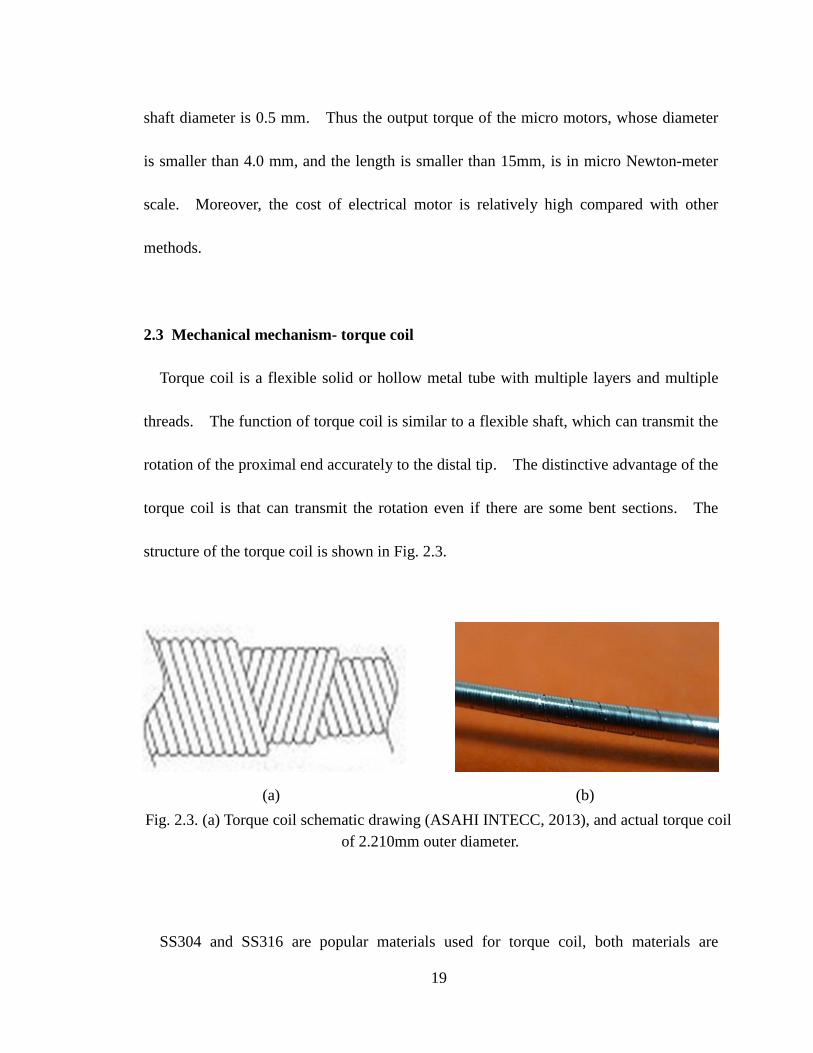
2.3 Mechanical mechanism- torque coil
Torque coil is a flexible solid or hollow metal tube with multiple layers and multiple
threads. The function of torque coil is similar to a flexible shaft, which can transmit the
rotation of the proximal end accurately to the distal tip. The distinctive advantage of the
torque coil is that can transmit the rotation even if there are some bent sections. The
structure of the torque coil is shown in Fig. 2.3.
SS304 and SS316 are popular materials used for torque coil, both materials are
Fig. 2.3. (a) Torque coil schematic drawing (ASAHI INTECC, 2013), and actual torque coil
of 2.210mm outer diameter.
(a) (b)

20
approved by FDA for medical device. Since during the sample cutting procedure the
power or action transmission shaft of the devices in body is bent, the rotation
transmission through the transmission shaft is nonlinear, bent and long distance, which is
difficult and a challenge for a conventional rotational transmission mechanism such as a
rigid shaft. However, the application of torque coils eliminates the difficulty. Besides,
the multiple sizes of the torque coils give the capability of integration with different
sample cutting devices. Table 2.2 shows two types of hollow torque coils supplied by
ASAHI INTECC.
Table 2.2. Major dimensions of the torque coil samples (ASAHI INTECC, 2013).
Sample O.D. (mm) I.D. (mm) Material Layer Length(mm)
Sample 1 1.950 1.420 SS304 1 2470.0
Sample 2 2.210 1.500 SS304 2 1955.0
Based on the information supplied by the manufacturer (ASAHI INTECC, 2013), the
accuracy of the rotational transmission between the proximal end and the distal tip is up
to 1:1, which means the rotation transmission is very accurate. However, there is no
information about the maximum rotation speed of the torque coil. A torque coil rotation
speed monitor system is set up, which is shown in Fig. 2.4. The proximal end of torque
coil is connected to an electrical motor. The distal tip of torque coil is connected to a

21
rigid shaft, which is exposed by a LED light. The LED controller is connected to the
function generator. The function generator sends a pulse signal to the LED controller,
thus the LED light is acting as a strobe light, and the frequency of the strobe light is
adjusted by the frequency of the pulse signal. When the frequency of the strobe light is
equal to the frequency of the rotation of the distal tip of torque coil, the rotation is
‘frozen’, which is captured by CCD camera, and the rotation speed is obtained. The rest
of torque coil is within a PVC tube. The inner diameter of the PVC tube is 2.33 mm.
The tests run at low rotation speed around 400 rpm and high rotation speed 1400 rpm.
The ‘frozen’ images are captured when the rotation speed are around 400 rpm, which are
shown in Fig. 2.5. Two samples are tested and the experimental results are shown in Fig.
2.6 and Fig. 2.7.
2 5 6
4 3 1
7
Fig. 2.4. Torque coil rotation speed measurement system: 1 are DC motor and DC motor
power supplier; 2 is the torque coil within PVC tube; 3 is LED controller; 4 is function
generator; 5 is LED; 6 is CCD camera;7 is PC.

22
T=0.15s T=0.3s T=0.45s
T=0.60s T=0.75s T=0.90s
T=1.05s T=1.20s T=1.35s
Fig. 2.5. Representative images of the distal tip of torque coil rotating at speed of 400
rpm captured by the camera in time interval of 0.15s. The capture time period is
determined by the strobe light frequency. When the strobe light frequency is equal to
the frequency of torque coil rotation, the captured images are the same, which is
“frozen”.

23
Fig. 2.6. Different rotational speed tests for finding the maximum
rotation speed of sample 1: (a) low rotation speed test, (b) high rotational
speed test.
(a)
(b)

24
Fig. 2.7. Different rotational speed tests for finding the maximum rotation
speed of sample 2: (a) low rotation speed test, (b) high rotational speed test.
(a)
(b)

25
From the experimental results, the rotation transmission is stable and uniform. No
delay or significant vibration is at the distal tip of the torque coil. In addition, the
rotation transmission is nearly linear. However, when the torque coil runs at rotation
speed of above 1400 rpm, there is a fluctuation, which may be explained that there is
some plastic deformation or torsion on the torque coil caused by the friction.
As the rotation speed increasing, the plastic deformation increases, and finally the
torque coils are failed at around 1800 rpm after 5 mins running. Fig. 2.8 illustrates the
failure of the torque coil tested in the system shown in Fig. 2.4. The failure location is
at the connection with the motor.
Thus, the accuracy of the rotation transmission of torque coil is up to 1:1, which
supplies a capability of an accurate rotation transmission from the proximal end to the
distal tip. However, when the torque coil rotates at high speed, there will be some
Fig. 2.8. Torque coil failed during the rotation test shown in
Fig. 2.4. The failure occurs at the connection with the motor.

26
torsion or failure, which should be taken into account when the high rotation speed
transmission is required.

27
3. Mechanics of cutting
The thesis focuses on the investigation of the power mechanisms for rapid rotational
cutting action in millimeter scale. Since the cutting geometry has influence on the
required cutting force or power, in this Section the theory of contact mechanics and
orthogonal cutting mechanics are used to find the relationship between the tool geometry
and the cutting force or power.
Based on the contact mechanics, the shapes of contact objects influence the stress
distribution and the location of first yield. Thus, the contact of a rigid sphere and a
deformable flat surface, as well as a rigid cone and a deformable flat surface are
investigated respectively in this Section in order to find the stress distribution under the
surface, and where the first yield occurs under the same pure normal load, which will be a
benefit to determine the cutting geometry.
3.1 Introduction
The cutting process is also the material elastic and plastic deformation, fracture and
removal process. There are three regions of material response to the compression of
cutting tool (Fischer-Cripps, 2007), which is shown in Fig. 3.1.
1. Region1 - Full elastic response, no permanent or residual impression left in the test
specimen after removal of load
2. Region2 - Plastic deformation exists but is constrained by the surrounding elastic

28
material
3. Region3- Plastic region extends and continues to grow in size and fracture or failure
occurs.
Fig. 3.1. A deformable plate responds to a normal load applied by a rigid cone: (a) a
normal load is applied, there is elastic deformation in the plate; (b) if the load is removed,
the deformation of plate recovers due to the elastic deformation; (c) the increment of the
load and contact lead the deformation to increase; (d) the plastic and elastic deformation
occur; if the load is removed, there is some elastic recovery; (e) the increment of the load
and contact lead to the plastic deformation increase and fracture occur; (f) there is fracture
occurring on the plate.
F
r
z
(a)
r
z
(b)
F
r
z
(c)
F
r
z
(e)
(d)
z
r
(f)
z
r

29
In the Region 1, during the initial application of load, the response is elastic and can be
predicted from the Hertz relation (Hertz, 1881).
Hertz contact problem is the study of contact between two continuous, non-conforming
solids. The contact between these two solids is initially a point or line. The sphere and
cone contact with the flat surface are introduced.
3.2 Axial symmetrical elastic analysis
In three dimensional contact problems, the axial symmetrical elastic analysis can be
simplified greatly by conversion to cylindrical polar coordinates ),,( zr . In the
contact problem, the hoop stress is always a principal stress, because of the
symmetry within the stress field. r ,
z and are independent of , and
0 zr . In the contact problem, it is convenient to calculate the principal stress in
the rz plane by the following equations (Fischer-Cripps, 2007):
2
2
3,122
rzzrzr
, (3.1)
2 , (3.2)
31max2
1 . (3.3)
30
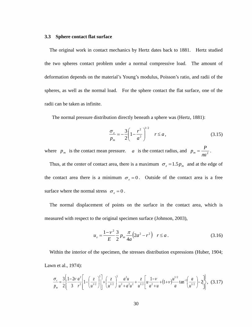
3.3 Sphere contact flat surface
The original work in contact mechanics by Hertz dates back to 1881. Hertz studied
the two spheres contact problem under a normal compressive load. The amount of
deformation depends on the material’s Young’s modulus, Poisson’s ratio, and radii of the
spheres, as well as the normal load. For the sphere contact the flat surface, one of the
radii can be taken as infinite.
The normal pressure distribution directly beneath a sphere was (Hertz, 1881):
ara
r
pm
z
2/1
2
2
12
3, (3.15)
where mp is the contact mean pressure. a is the contact radius, and 2a
Ppm
.
Thus, at the center of contact area, there is a maximum mz p5.1 and at the edge of
the contact area there is a minimum 0z . Outside of the contact area is a free
surface where the normal stress 0z .
The normal displacement of points on the surface in the contact area, which is
measured with respect to the original specimen surface (Johnson, 2003),
arraa
pE
u mz
222
242
31 . (3.16)
Within the interior of the specimen, the stresses distribution expressions (Huber, 1904;
Lawn et al., 1974):
2tan1
11
3
21
2
32/1
12/1
22/1222
23
2/1
3
2/12
2
u
a
a
u
uau
u
z
uau
ua
u
z
u
z
r
a
pm
r
, (3.17)

31
2tan11
13
21
2
32/1
12/1
22/1
3
2/12
2
u
a
a
u
uau
u
z
u
z
r
a
pm
, (3.18)
222
23
2/12
3
zau
ua
u
z
pm
z, (3.19)
2
2/1
222
2
2
3
au
au
zau
rz
pm
rz, (3.20)
where
2/1222222222 4
2
1zaazrazru .
Because this problem is an axis-symmetric problem, the principal stress in rz plane
could be solved by the Eqs 3.1 to 3.3. The distribution of maximum shear stress and
von Mises are shown in Fig. 3.2 and Fig. 3.3, respectively.
The stresses along z-axis are calculated from (Johnson, 2003):
1
2
21
00
12
1tan11
a
z
z
a
a
z
pp
r , (3.21)
1
2
2
0
1
a
z
p
z, (3.22)
where 0p is the maximum contact pressure
Based on the equation 3.21 and 3.22, the stress distribution along the depth below
contact area could be observed in Fig. 3.4. It is shown the maximum shear stress and
von Mises located below the contact area, which means that the point of first yield is
hidden beneath the surface. For Poisson’s ratio 3.0 , the location is az 49.0 .

32
Fig. 3.2. Contour of equal maximum shear stress for spherical contact calculated for
Poisson's ratio . Distances r and z normalized to the contact radius a and
stresses expressed in terms of mean contact pressure.

33
Fig. 3.3. Contour of equal von Mises stress for spherical contact calculated for
Poisson's ratio . Distances r and z normalized to the contact radius a and
stresses expressed in terms of mean contact pressure.

34
Fig. 3.4. The ratio of stress distribution to contact pressure along z-axis below the
contact area of the contact between a sphere and a flat surface for Poisson’s ratio
3.0v .
z/a

35
3.4 Rigid cone contact surface
Rigid cone contact surface is hot practical interest because this is used for material
hardness tests. The displacement of points in the contact area measured with respect to
the original specimen free surface is given by (Sneddon, 1948):
araa
ruz
cot
2, (3.23)
where a is the contact radius.
The pressure distribution on the face of the cone (Johnson, 2003):
)/(1coshcot)21(2
)( raE
rp
, (3.24)
where is the cone semi-angle, E is the specimen Young’s modulus, and is the
specimen Possion’s ratio.
Equation 3.24 shows that a theoretically infinite pressure exists at the apex. By
considering the variations in stress along the z-axis, the principal shear stress (Johnson,
2003) is:
122cot2
2122
1
zaaE
zr
. (3.25)
There is a maximum yet finite value
cot212
E
at the apex. In this case
two principal stresses r , so that the von Mises criteria are identical if expressed
in term of Y, where Y is the yield, or flow stress, of the specimen. Thus yield will

36
initiate at the apex if the cone angle is such that
YE
cot21
. (3.30)
Thus for incompressible material, there is hydrostatic pressure combined with a finite
shear at the apex.
Hence, in the Region 1 - full elastic response of the specimen, the contact pressure
cot21
E
p , depends only on the cone angle and is independent of the load. Thus
the contact pressure increases with the decreasing cone semi-angle, which could explain
the sharper cutting tool have a better cutting performance.
The ratio of stresses to 21
E along the z-axis when the contact radius is 1.0 mm,
and the cone semi-angle is 30 is plotted in Fig. 3.5. The von Mises stress distribution
with different cone semi-angle when the contact radius 1.0 mm is shown in Fig. 3.6.

37
Ra
tio
of
stre
ss t
o
Depth below the contact surface
Fig. 3.5. Conical contact stress distribution along z-axis for cone
semi-angle of 30.
Ra
tio
of
stre
ss t
o
Depth below the contact surface
Fig. 3.6. Conical contact von Misese stress distribution of von Mises along
z-axis for cone semi-angle of 15, 30, 45and 60, respectively.

38
However in Region 3, the plastic material is no longer elastically constrained, and the
plastic strains are large compared with the elastic strains, the elastic deformation maybe
neglected. Thus, it could be taken as a rigid-perfectly-plastic solid. Plastic yield in
such a material depends upon a critical shear stress which may be calculated using von
Mises failure criteria. In the slip-line field solution, assuming there is frictionless
contact between the compression tool and specimen. The material in the region ABCDE
flows upward and outward as the tool moves downward under load. Because there is no
friction, the direction of stress along the line AB is normal to the face. The lines in the
region ABCDE are oriented at 45 to AB and are called ‘slip lines’ as shown in Fig. 3.7
(Fischer-Cripps, 2007).
If the tool penetrates the specimen with a constant velocity and the geometrical
Fig. 3.7. Slip-line theory in two dimensions by Hill et al., 1947,
(Fischer-Cripps, 2007).

39
similarity is maintained, the angle can be chosen so that the velocities of element of
material on the free surface, contact surface, and boundary of the rigid plastic material are
consistent. The contact pressure across the face of the tool is given by (Fischer-Cripps,
2007)
112 max Ypm , (3.31)
where
project
mA
Pp .
For a conical tool, the projected area projectA is depend of ch and tan . ch is the
depth of penetration measured from the area of contact. Thus for a certain material, as
the tool semi-angle decreases, the load for cause the specimen deforming and fracturing
decreases, which could explain the cutting tool geometry could affect the cutting force.
3.5 Orthogonal cutting
There are three major ways the cut geometry can be classified: orthogonal, oblique,
and three dimensional cutting. Orthogonal cutting uses a single cutting edge, and the
velocity of the work-piece material V, is orthogonal to this cut edge.
In this Section, the cutting force is analyzed based on De Vries’ model, 1991, where
the orthogonal cutting mechanics is employed (De Vries, 1991). Furthermore based on
the knowledge of cutting operation such as tool geometry, cutting condition (i.e. depth of
40
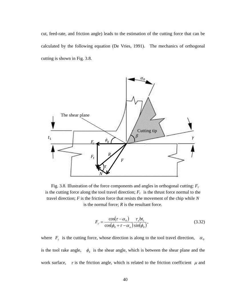
cut, feed-rate, and friction angle) leads to the estimation of the cutting force that can be
calculated by the following equation (De Vries, 1991). The mechanics of orthogonal
cutting is shown in Fig. 3.8.
0
1
0
0
sincos
cos
btF s
o
c
, (3.32)
where cF is the cutting force, whose direction is along to the tool travel direction, 0
is the tool rake angle, 0 is the shear angle, which is between the shear plane and the
work surface, is the friction angle, which is related to the friction coefficient and
𝛼0
𝑡1 𝛾 𝐹𝑐
𝐹𝑡 𝑅
The shear plane
𝐹
𝑁
0
𝜏
Cutting tip 𝛽
Fig. 3.8. Illustration of the force components and angles in orthogonal cutting: Fc
is the cutting force along the tool travel direction; Ft is the thrust force normal to the
travel direction; F is the friction force that resists the movement of the chip while N
is the normal force; R is the resultant force.

41
1tan , 1t is the underformed chip thickness or depth of cut, b is the uncut chip
width in three dimensional cutting, S is the material shear strength under cutting
conditions.
The shear plane angle can be predicted by Ernst-Merchant model or Lee-Shaffer model.
The first model is based on the minimizing force and Lee-Shaffer model is based on slip
line theory.
The criterion used by Ernst and Merchant, 1941, was to select 0 so as to minimize
the magnitude of the resultant force. The predicted shear angle is (Ernst and Merchant,
1941),
2
0450
. (3.33)
The shear plane angle is predicted by Lee-Shaffer (Lee and Shaffer, 1951) is,
00 45 . (3.34)
The friction angle 1tan where is the friction coefficient, thus for the same
cutting condition, the friction coefficient keep same. For the positive rake angle, there is
a relationship between positive rake angle, tool angel, and the flank angle.
o90 , (3.35)
where is the tool angle, is the flank angle. Thus as the rake angle increases, the
shear angle increases, then the cutting force decreases.

42
3.6 Two-dimensional photo-elastic fringe patterns of rigid cones
From the previous discussion, the location of first yield due to the contact between a
cone and a flat surface is on the surface and nearby the apex of the cone. To observe the
live stress distribution and failure caused by a conical contact, a photoelasticity system is
set up. The two-dimensional photo-elastic fringe patterns of rigid cones are captured as
a function of increment in the contact load. The rigid cone tool model with the
semi-angle 30 is made from stainless steel. A normal load is applied and the rigid cone
tool contacts the elastic plate which is made from Lexan polycarbonate sheet. Figure
3.10 shows the development of the stress fringe patterns as a function of increment in the
contact load. The cone penetrates the plate with a velocity 0.02 mm/ time. The
location of the facture of the elastic plate is on the rigid surface.
LED Polarizer
Analyzer
CCD
camera
Collimating
lens
Quarter
waverplate
Fig. 3.9. Photoelasticity system developed at CHLST labs.

43
Fig. 3.10. Photoelastic stress fringe patterns of rigid cone: a pure normal load is applied
by a rigid cone with semi-angle of 30. As the load is increased, the number of fringes
representing the stress distribution within the plate increases, as shown from (a) to (i).
(a) (b) (c)
(h) (i) (g)
(f) (d) (e)

44
4. Finite element analysis
4.1 Introduction
Cutting process is a very complicated; it is influenced by the material mechanical
properties, failure property, cutting tool geometry, cutting speed, depth of cut and width
of cut, as well as the friction between cutting tool and the specimen. During the cutting
process, the friction between cutting tool and specimen also causes the thermal
conductivity. Researchers are trying to find the best cutting conditions and tool
geometries to optimize process efficiency. Although the results could be obtained by
experimental works, they are time-consuming and expensive. In addition, simple
analytical methods have limited application to explain the cutting process. Thus,
numerical methods are becoming more important.
4.1.1 Introduction of Abaqus
In recent years, commercial finite softwares such as Abaqus, ANSYS, COMSOL, etc.
have been used popularly in academic and industrial areas for computer-aided design and
analysis. Because the cutting analysis is a complicated dynamic analysis involving
contact, plasticity, large deformation and element failure, the commercial finite software,
which has a significant application for nonlinear dynamic and high deformation problems,
is required. Abaqus was first released in 1978 including three main analysis products:
Abaqus/Standard, Abaqus/Explicit, and Abaqus/CFD. Abaqus/Standard is popularly
45
used for static equilibrium problem in structural simulations while Abaqus/Explicit is
better in applications for the nonlinear dynamic and high deformation problems.
Abaqus/CFD is a computational fluid dynamic analysis package. Based on the
requirements of the cutting process analysis, Abaqus/Explicit is used for the analysis.
In this Section, the procedure of finite element analysis in Abaqus and some critical
problems are presented. The finite element results are compared with the analytical
results for verifications.
4.2 Chip separation criterion
4.2.1 Finite element approach
In finite element methods, the displacement-based finite element analysis is used
popularly since it reduces computational time. In this Section, the basic equations for
standard displacement-based finite element analysis are described (Abaqus, 2013).
Let f be the vector of displacement at any point of the element, and the vector of
nodal displacements of an element could give the vector of displacement at any point of
the element by interpolation functions
eNf , (4.1)
N is the matrix of shape functions serving as interpolation function, and e is
the vector of nodal displacements at any point of the element.
From the linear elastic mechanics, the element strain is associated with the nodal
46
displacement of an element
eB , (4.2)
is the vector of strain at any point of the element and B is the
strain-displacement matrix that transforms nodal displacement to strains at any point in
the element.
The stresses in individual elements is given as
eBD , (4.3)
is the vector of stress at any point of the element and D is the elastic matrix
related to the material elastic properties.
According to the virtual work principle, the work-equivalent nodal force could be
given
eeekF , (4.4)
where eF is the work-equivalent nodal force vector and ek is the element
stiffness matrix.
Using the direct stiffness method, combine the elements and get the entire structure
stiffness matrix and all elements equivalent nodal force vector. Since the nodal
displacement at the common nodes in the neighbor elements is same, the structure
stiffness matrix k , the force vector F and the nodal displacement vector of all
elements could be related as
kF . (4.5)
47
Thus, in the finite element analysis, the nodal displacement in the structure could be
used to get nodal displacement at any point in the element, then get the stress at any point
in the element.
4.2.2 Element failure model
The process of cutting is the process of material dynamic failure process. Abaqus
supplies two element failure models: shear failure model and tensile failure model. The
shear failure model uses the equivalent plastic strain as a failure measure. The tensile
failure model uses the hydrostatic pressure stress as a failure measure to model dynamic
spall or pressure cutoff. In this Section, the shear failure model is used to analyse the
cutting process.
The shear failure model is based on the value of the equivalent plastic strain at element
integration points; failure is assumed to occur when the damage parameter exceeds 1. The
damage parameter, , is defined as
pl
f
plpl
, (4.6)
where pl
is any initial value of the equivalent plastic strain. pl
is an increment of
the equivalent plastic strain and pl
f is the strain at failure (Abaqus, 2013).

48
4.2.3 Element removal
When the shear failure criterion meets at an integration point, all the stress components
will be set to zero and that material point fails. By default, if all of the material points at
any one section of an element fail, the element is removed from the mesh. The cutting
model using the splitting line is defined for the cutting process analysis. This model
contains 4 parts: cutting tool, uncut chip, splitting line, and base, which are shown in Fig.
4.1. The uncut chip, splitting line, and base are considered as a single part and defined
the specimen. Define the fracture stress/strain as the shear failure criterion to the
splitting line, thus when the plastic deformation of the element of the splitting line meets
the shear criterion, the element is removed leading to the chip separating from the base.
For an accurate failure model, the material elastic and plastic properties are necessary.
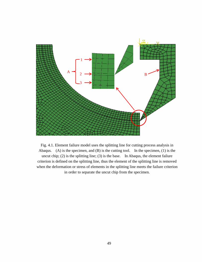
49
1
2
3
Fig. 4.1. Element failure model uses the splitting line for cutting process analysis in
Abaqus. (A) is the specimen, and (B) is the cutting tool. In the specimen, (1) is the
uncut chip; (2) is the splitting line; (3) is the base. In Abaqus, the element failure
criterion is defined on the splitting line, thus the element of the splitting line is removed
when the deformation or stress of elements in the splitting line meets the failure criterion
in order to separate the uncut chip from the specimen.
A B

50
4.3 Model definition
In the cutting model using splitting line, there are 4 parts including uncut chip, splitting
line, base, and cutting tool.
The cutting tool geometry is shown in Fig. 4.2(a). The height of the cutting tool is
1.0mm. The rake angle is 200 , the tool angle is 30 , and the flank angle is
40 .
The uncut chip thickness is uniform, which is 0.1 mm, and the angle is 90, which is
shown in Fig. 4.2(b). The splitting line thickness is also uniform, which is 0.01 mm,
and the angle is 90 as shown in Fig. 4.2(c). The base height is 3.0 mm and length is 3.0
mm, and the angle is 90.

51
𝑂
Fig. 4.2. Cutting tool geometry: (a) the cutting tool; (b) the uncut chip; (c) the
splitting line.
30
20
40
𝟏.𝟎𝐦𝐦
𝑂
(a)
𝐫 =0.89mm
𝑂
𝐑 =0.99mm
(b)
𝐫 =0.99mm
𝐑 =1.0mm
(c)

52
4.4 Material properties definition
In Abaqus, to simulate the cutting process, the material model must have defined the
mass density, elastic or hyperelastic properties, plastic stress-strain, and the failure
criterion. In this Section, the structure and hyperleastic properties of a representative
biological sample are presented. However, because of the limited information about the
plastic stress-strain and the failure criterion of biological samples a linear elastic and
linear plastic material model is utilized in the cutting process simulations.
4.4.1 Biological samples structure and mechanical properties
As the medical development, the structure and mechanical properties of biological
sample are required for the development of medical device and therapies. In recent
years, more and more researches about the biological sample mechanical properties are
being released.
A representative biological sample, for example, the soft representative biological
sample is a group of tissue which binds, supports and protects body and structures and
organs, for example, tendons, blood vessels and skin (National Cancer Institute, 2013).
They are distinguished from hard tissue such as bones for their high flexibility and soft
mechanical properties.
The fiber-reinforced composite structures are the main characteristic of the soft
representative biological sample and their mechanical behavior is strongly influenced by

53
the concentration and structural arrangement of constitute such as collagen and elastin
(Fung, 1993).
The soft representative biological sample behaves anisotropically, since the fibers have
preferred directions. In a microscopic sense they are non-homogeneous materials
because of their composition. The tensile response of the soft representative biological
sample is nonlinear stiffening and tensile strength depends on the strain rate. In contrast
to hard tissues, the soft biological sample may undergo large deformations. Even
though some soft biological samples have hyperelastic properties, the stress-strain curve
is a typical J-shaped (tensile), as shown in Fig. 4.3.
Fig. 4.3. Load-elongation curve for a ligamentum flavum
tested in tension to failure (Nachemson and Evans,
1968).

54
4.4.2 Limitation of modeling biological sample fracture in Abaqus
In Abaqus, there are two methods to define a hyperelastic material model, which are
tensile or shear experiment data and the stain energy potential defining the strain energy
stored in the material per unit of reference volume as a function of the strain at that point
in the material. The strain energy potentials models include Ogden and Mooney-Rivilin
for hyperelastistic material. However, for the large deformation and element failure
analysis, the plastic stress/strain, an element failure criterion, must be defined in Abaqus,
there are few publications about the plastic deformation, stress and failure. Thus, the
material model is not totally defined and the analysis cannot be conducted. For the
cutting analysis, a linear elastic and linear plastic material model is defined in Section
4.4.3.
4.4.3 Material properties definition
In Abaqus, when the element deformation or stress meets the shear failure criterion, the
element is removed in order to obtain the chip separated from the original model. Thus
the original model, which is nominated as specimen in previous section, contains uncut
chip, splitting line and the base. Define the failure criterion to the splitting line. Then,
when the elements in the splitting line meet the criterion, the elements are removed and
the chips fall off. The mass density of the specimen is assumed to be 3/8250 mkg , the
Young’s modulus Pa8102.2 , and the Poisson’s ratio 0.3, as recommended in Fung,

55
1993. The plastic stress-strain is linear, Fig. 4.4.
The linear elastic and linear plastic material model is not appropriate and unrealistic
definition for the biological material, which has high density and elasticity modulus.
However, the cutting analysis is a complicated dynamic analysis involving contact,
plasticity, large deformation and element failure, there will be significant mesh distortions
causing the instability of the analysis during the analysis. Due to the influence of the
Fig. 4.4. Definition of material plastic stress-strain in Abaqus. Abaqus splits
the material elastic and plastic stress strain curve into two separate parts including
elastic stress-strain curve and plastic stress-strain curve. The plastic strain starts
from 0.

56
material properties including the mass density, elastic properties, and plastic property to
the analysis stability, a material model with appropriate definition is required. Several
material models are used, and the above material model gets a relatively stable result,
which is not appropriate definition for a biological material but a required procedure.
For modeling purposes only and to insure rigidity, the cutting tool density is assumed
to be 3/15000 mkg . In contrast to the specimen, the Young’s modulus of the cutting
tool is Pa12100.8 and the Poisson’s ratio is 0.2. Thus, the cutting tool is rigid, and it
does not undergo any deformations. The comparison of the materials’ properties is
shown in Table 4.1.
Table 4.1. Comparison of assumed specimen and cutting tool material properties.
Specimen Material
Properties
Cutting tool Material
Properties
Mass density (3/ mkg ) 8250 15000
Young’s modulus (Pa) 8102.2 12100.8
Poisson’s ratio 0.3 0.2
For modeling purposes only. For more specifics see Fung, 1993.

57
4.5 Definition of mesh
4.5.1 Definition of mesh element type
Finite element analysis is the method that the geometry under consideration is divided
in large number of small elements. In two-dimensional analysis, the triangles or
quadrilaterals are used typically as shown in Fig. 4.5.
In two-dimensional stress/displacement analysis, Abaqus supplies continuum elements
for complex nonlinear analyses involving contact, plasticity, and large deformations.
For the stress/displacement analysis, element CPS4R is selected, which is a 4-node
bilinear plane stress quadrilateral, reduced integration, hourglass control element type
(Abaqus, 2013). For a reduced-integration element, the displacement solution is more
accurate and the analysis accuracy is not affected even when the mesh has a significant
distortion (Abaqus, 2013). In contrast to the full-integration element, the
reduced-integration has only one integration point; the stress on the integration point is
Fig. 4.5. Finite elements: (a) the triangle element; (b) the quadrilateral element.
P1
P3 P4
P2 P1
P2 P3 (a) (b)

58
relatively accurate. The difference between full-integration element and
reduced-integration element is shown in Fig. 4.6.
4.5.2 Definition of mesh element size
In order to find the influence of the element size to the accuracy of the analysis result,
three meshing models are conducted. The numbers of elements of these three meshing
models are shown in Table 4.2.
Fig. 4.6. Integration elements: (a) full-integration element; (b)
reduced-integration element.
P3
P2 P1
P4
I1
P1 P2
P4 P3
I1 I2
I4 I3
(a) (b)

59
Table 4.2. Number of elements in three meshing models.
The finite element results shown in Fig. 4.7 reveal that for different meshing models,
the cutting force is almost same. In contrast, the stability of the result is affected by the
meshing models. There are significant fluctuation on the results of model 1 and model 3,
and the result plot of model 2 is relatively smooth. Thus, considering the accuracy and
stability of the finite element analysis result, the meshing model 2 is selected, which
defines the mesh size.
Model Number of elements Total number of
elements Uncut chip Splitting line Base
Model 1 320 80 3330 3730
Model 2 400 100 4001 4501
Model 3 480 120 4554 5154

60
4.6 Definition of boundary condition
4.6.1 Surface contacts
4.6.1.1 Surface contacts in specimen
There are two pairs of surface contact between the parts in specimen, which are uncut
chip bottom surface and the splitting line up surface, as well as, the splitting line bottom
surface and the base up surface. These surface contact properties are same. The
surface contact tangential friction is “Rough” leading to no slip will occur as long as the
surfaces are in contact and in the normal contact “don’t allow the separation after contact,”
(Abaqus, 2013).
Fig. 4.7. Finite element results of three meshing sizes.

61
4.6.1.2 Dynamic surface contacts between cutting tool and specimen
The contact between the cutting tool and the specimen is a dynamic contact. Assume
the tool is rigid body and the specimen is deformable. The dynamic contact is the
interaction between a deformable body and a rigid body.
A is a point on the deforming mesh of specimen with current coordinate AX . C is a
point in the cutting tool with the current coordinate CX . 'A is the closest point on the
surface of the cutting tool to A at which the normal to the surface of the cutting tool, n ,
pass through A. r is the vector from C to 'A . The geometry described is shown in
Fig. 4.8. Define the distance between A and 'A is h. From the definitions introduced
above

62
𝐴
𝐴′
𝐶
Fig. 4.8. Illustration of dynamic contact between tool and specimen.
rXXhn CA
. (4.7)
Define c is the clearance below which contact occurs. If ch , the surfaces are not
in contact at A, no surface interaction calculations need be done at this point. For a
“Hard” contact 0c in Abaqus. If ch , the surface are in contact.
When point A and the cutting tool are moving, point 'A is moving on the surface of
the cutting tool. The movement of point 'A consists of two parts: movement due to
motion of the cutting tool and motion relative to the body. S is the measure distance

63
along the tangents t to the surface at 'A .
trXrrXX CCCCA , (4.8)
where is the ‘slip’ of point 'A , and the normal n will also change due to rotation
of the cutting tool surface and due to slip along the surface.
S
nnnnn nC
. (4.9)
Substitution of Eq. 4.8 and Eq. 4.9 to Eq. 4.7, the linearization form of the contact
equation becomes
trXX
S
nnhhn CCAC . (4.10)
For “Hard” contact 0h , the linearized kinematic Eq. 4.10 becomes
trXXhn CCA . (4.11)
This equation could be split into normal and tangential components,
CCA nrXXnh , (4.12a)
CCA trXXt . (4.12b)
For dynamic cutting analysis, the velocity and acceleration terms h and h are used
to calculate impact forces and impulse correctly.
rXXnh CCA , (4.13a)

64
rXXtS
nnrXX
rnrnrXXnh
CCACCCA
CCCCCCA
. (4.13b)
4.6.2 Node constrain of the specimen
The definition of boundary condition of the specimen is shown in Fig. 4.9. All the
degrees of freedom of the nodes at the edges, which don’t contact with the cutting tool,
are constrained. Thus, during the cutting process the dynamic contact between the
cutting tool and the specimen will not make the specimen moving.
Fig. 4.9. Definition of boundary condition of the specimen in Abaqus: the
constraint of all degree of freedom of the nodes at the specimen’s edges makes sure
the specimen not to move during the cutting process.

65
4.7 Definition of load condition
Reference Point (RP) is used to apply the load (Abaqus, 2013), which is shown in Fig.
4.10. Apply rotation speed to the reference point in order to lead the cutting tool to
rotate taking the reference point as the rotation center. No translation in both x-direction
and y-direction. The distance from the Reference Point to the tip of the cutting tool is
1.0 mm. The rotation/displacement is 2 radians/0.01s, which is around 1900 rpm. The
load period or step is 0.012 s.
RP
Fig. 4.10. Definition of load condition in Abaqus. Reference
point is used to apply the load in Abaqus. In the rotational cutting
process, the rotation speed is applied to the RP, and the tool rotates
taking the RP as the rotation center at the applied rotation speed.

66
4.8 Stability analysis
The explicit procedure integrated through time by using many small time increments.
Stable time increment is the one that leads to the convergence of analysis. In explicit
dynamic analysis, the stable limit for the analysis is given in terms of the highest
frequency max of the system as (Abaqus, 2013):
max
2
t . (4.14)
However, the actual highest frequency in the system is based on a complex set of
interacting factors, and it is not computationally feasible to calculate its exact value. In
Abaqus/Explicit, an alternative method is used to estimate the stable time increment.
The stable time increment is grossly estimated using the element length eL and the wave
speed of the material dc
d
e
c
Lt , (4.15)
where
Ecd . E is Young’s modulus and is the mass density. Thus as the
number of elements increases for a specific model, the stable time limit decreases, which
is shown in Table 4.3.

67
Table 4.3. Stable time increment of the models with different element sizes in Abaqus.
4.9 Results and discussions
The cutting tool with rake angle 200 , tool angle 30 , and flank angle
40 . The height of the cutting tool is 1.0 mm. The distance between the cutting
tip and the Reference Point is 1.0 mm. Apply the boundary condition of the rotation
displacement/load to the Reference Point. The rotation boundary condition is 2
radians/0.01s, thus the rotation speed is around 1900 rpm, and the time period or step is
0.012s. The uncut chip thickness is 0.1 mm and length around 6.28 mm. The mesh
element is CPS4R, which is a 4-node bilinear plane stress quadrilateral, reduced
integration, hourglass control element type. There are 135 elements in cutting tool.
Splitting line contains 100 elements, and 400 elements are in the uncut chip. In addition,
there are 4001 elements in base. Define the shear failure criterion to the splitting line in
order the chip separating the specimen when the cutting force is applied. The specimen
Model Number of elements Total number of
elements
Max
∆𝒕𝒔𝒕𝒂𝒃𝒍𝒆(𝒔) Uncut chip Splitting line Base
Model 1 240 60 2740 3040 5.02e-08
Model 2 320 80 3330 3730 4.56e-08
Model 3 400 100 4001 4501 4.13e-08
Model 4 480 120 4554 5154 3.34e-08

68
is deformable and the cutting tool is rigid. The magnitude of cutting force along time is
shown in Fig. 4.11.
O
AB
C
Fig. 4.11. Finite element result of the magnitude of the cutting force when the cutting tool
rotation speed is 1900 rpm, and the uncut chip thickness is 0.1 mm. Point O represents the
cutting tool contacts the specimen. From point O to point A, as the increment of the contact
between the cutting tool and the specimen, the magnitude of stress on the contact surface is
increasing due to elastic deformation. Point A represents the contact force is up to the ultimate
stress. From point A to point B the force is up to material ultimate stress, the material is
removed continuously till all the material is removed. From point B to point C, since the
material is removed, and there is little or no contact between the cutting toll and the specimen,
the magnitude of the cutting force decreases.

69
4.9.1 Fluctuations in the curve
The magnitude of cutting force is the stress or force on the integration point of each
element in the splitting line when the integration point of the element meets the failure
criterion, and the element is removed. In this analysis, the reduced-integration element
is used and there is only one integration point in each element. Since the element failure
is instantaneous and the failure happens element by element, thus the stress on the
integration point of the element is output one by one, which is not constant leading to
some fluctuations in the curve (Zhang et al, 2008).
4.9.2 Cutting process regions
The total cutting time is 0.0078 s, and there are three regions in the cutting process
according to the material elastic/plastic deformation and fracture as shown in Fig. 4.11.
Region 1 is from point O to around point A. As the contact between the cutting tool
and the specimen increases, the magnitude of stress on the contact surface is increasing
and the deformation is elastic and plastic. Since the material mechanical property is
linear elastic and linear plastic, the magnitude of contact stress is increasing linearly.
Region 2 starts from around point A to point B, where the elements are removed. As
the cutting tool is keeping contacting the specimen, the magnitude of contact stress is
increasing and the deformation is increasing too. When the contact stress or strain is up
to the ultimate stress or ultimate strain, the material starts fracture or failure, thus the

70
elements in the splitting line are removed and the chip is separated from the base. The
stress on the integration point of each element is the required stress or force to removing
the material from the specimen.
Region 3 is from point B to point C, where the chip is separated from the specimen and
the there is little or no contact between the cutting tool and the specimen. Thus the
cutting force is decreasing. The material response and the cutting action are shown in
Fig. 4.12.
(a) (b)
(d) (c)
Fig. 4.12. Material deformation and fracture during the cutting process:
(a) the cutting tool contacts the specimen, and there is elastic and plastic
deformation in the specimen; (b) as the increment of contacts between the
cutting tool and the material, the specimen starts to fracture; (c) the chip is
almost separated from the specimen; (d) the chip is totally separated from
the specimen.

71
4.10 Rake angle analysis
The cutting tool rake angle is changing from 10, 20 to 30, where the flank angle
keeps 40. Thus the cutting tool angle is decreasing from 40, 30 to 20. The
simulations are running respectively at rotation speed around 1900 rpm. According to
the previous theoretical study, as the tool angle decreases, the force causing the
elastic-plastic deformation and facture decreases. The finite element analysis results
plot in Fig. 4.13.
Fig. 4.13. Comparison of magnitude of cutting force of the cutting tools with rake angle
10, 20, and 30 when the cutting rotation speed is 1900 rpm, and the uncut chip
thickness is 0.1 mm.

72
Table 4.4 shows the comparison of finite element analysis results and analytical result
from Eq. 3.32. In Eq. 3.32, s is the material’s shear stress under cutting condition.
In Abaqus, the material’s failure model is defined by the shear stress/strain, thus when the
material shear stress/strain is up to the shear stress/strain, the material is removed. Thus
s is equal to the model shear failure stress.
In addition, the entire model is in millimeter scale, for 2-dimensional simulation, the
width of cutting is 1.0 mm. The depth of cutting is 0.1 mm, which is defined in Chapter
3. Thus, the analytical and FEM cutting force results are shown in Table 4.4.
Table 4.4. Comparison of analytical and FEM results of the magnitude of
the cutting force.
Rake angle 10 20 30
Average cutting force by FEM (N) 4.47 3.68 2.39
Ratio of FEM results to the FEM result of the
model rake angle 10
1 0.8233 0.5347
Cutting force by orthogonal cutting method in
Chapter 3 (N)
4.70 3.92 3.23
Ratio of analytical results to the analytical result of
the model rake angle 10 in Chapter 3
1 0.8340 0.6872
Error FEMFEManalytical FFF /)( 0.05 0.07 0.35

73
Thus, when the rake angle is increasing and the tool angle is decreasing, the required
load for achieving the yield criterion is decreasing, which is same as the conclusion using
contact mechanics in Chapter 3.

74
5. Preliminary biological sample cutting experiments
The preliminary biological sample cutting experiments are conducted to find the
characters of the biological sample cutting and the influence of the rake angle of the
cutting tool on the cutting force.
5.1 Experiment system set up
The major components of the experiment are electrical motor, a torque coil, two torque
transducers, and tested cutting tool. The scheme of the experiment set-up is shown in
Fig. 5.1.
The torque transducer between the electrical motor and the torque coil is used to record
the motor torque and the torque transducer between the torque coil and the cutting tool is
used to monitor the cutting torque.
Electrical
motor
Torque
transducer
Cutting
tool Connector
Torque
coil
Torque
transducer
Fig. 5.1. Scheme of preliminary biological sample cutting experiment using torque coil as
the power transmission for the rotational cutting actions.

75
5.2 Biological sample cutting experiment result
The cutting tool with a flat or straight cutting edge was test at rotation speed 1000 rpm.
The outer diameter is 3.5 mm. During the cutting process, the data of torque was
captured versus times. The cutting toque was recorded by the torque transducer
between torque coil and the cutting tool. The plot of cutting torque versus time is
shown in Fig. 5.2.
Fig. 5.2. Raw experimental data from preliminary biological sample cutting
experiment at rotation speed 1000 rpm. “Event” represents the instant when the tool
contacts the sample.
-23
-21
-19
-17
-15
-13
-11
-9
-7
-5
0.1 1.1 2.1 3.1 4.1 5.1 6.1 7.1
Torq
ue
: mo
tor
(mN
m)
Time (s) Event

76
The experiment data reveals that the cutting path appeared to be formed by a repeated
sequence of localized deformation followed by localized fracture. When the cutter
contacts the sample, the magnitude of torque increased as the sample deformation
reached a peak, then the magnitude of torque suddenly dropped as onset of localized
fracture extension occurred, which corresponds with the finite element analysis results, as
shown in Fig 4.11.
5.3 Biological sample cutting experiments of using different cutting tools
Two different cutting tools were used in the preliminary biological sample cutting
experiments, which is shown in Fig. 5.3. Both tools’ outer diameter is 2.6 mm. The
length of cutting window is 4.0 mm and the width of cutting window is around 2.0 mm.
The tools’ geometries are listed in Table 5.1.
Fig. 5.3. Cutting tools used in experiments: (a) Tool A with a flat cutting edge, (b)
Tool B with a teeth cutting edge. The outer diameter of both tools is 2.6 mm. The
length of the cutting edge is 4.0mm, and the width of cutting window is
2.0 mm.
(a) (b)

77
The cross sections of cutting tips of two cutters are shown in Fig. 5.4. The rake angle
of Tool A is around 90 and the rake angle of Tool B is around 55. The experiments
focus on the influence of the rake angles of cutting tool on the cutting torque or force.
The torque data versus time is captured by the torque transducer between the torque coil
and the cutting tool. The results are shown in Fig. 5.5.
Table 5.1. Cutting tools geometries of tested tools.
Cutting
tool
O.D.
(mm)
I.D.
(mm)
Cutting window Tool angle
(degree) Height(mm) Width(mm)
Tool A 2.6 2.0 4.0 2.0 90
Tool B 2.6 2.0 4.0 2.0 55
Fig. 5.4. Cross section of the cutting edge of the tested tools: (a) Tool A;
(b) Tool B. The cutting tool geometries are shown in Table 5.1.
(a) (b)
0.1mm

78
The magnitude of cutting torque of Tool B is smaller than the magnitude of cutting
torque of Tool A, and the rake angle of Tool B is smaller than the rake angle of Tool A.
The experimental result is same as the analytical and finite element analytical result.
Fig. 5.5. Experimental results of the cutting torque for one revolution obtained by
tested tools at rotation speed of 3000 rpm. “Event” represents the instant when the
tool contacts the sample.
14
Time (ms) Event
Torq
ue
(m
Nm
)
0 5 10 15 20 25 10
11
12
13
15
16

79
6. Conclusions and discussions
Sample cutting is one of the important minimally invasive medical treatments. The
sample cutting at the distal end of the devices is achieved by the power or cutting action
transmission from the proximal tip to the distal end of the devices. Thus, for a
biological sample cutting during a minimally invasive surgery, the transmission of the
power or a cutting action from the proximal tip of the removal devices to the cutter at
the distal end is crucial.
However, since the minimally invasive procedure is processed by inserting the
devices into patient’s body from a tiny aperture, the common characteristic of the sample
cutting devices are long and slim. For example, the working length of the TurboHawk
system is from 1100 mm to 1450mm, and the diameter is from 1.9 mm to 2.7mm. The
length of the endoscopes working channel, which allows the endoscopic devices, for
example, biopsy forceps, to pass through, is up to 2180 mm, and the diameter is from
0.75 mm to 6.0 mm.
The challenge of the sample cutting in the minimally invasive medical treatment is that
enough power must be transmitted to the cutter at distal end of the devices for biological
sample cutting, whose length is up to meters, and the diameter is in millimeters scale.
Thus, an investigation of the potential powering mechanisms was conducted.
In addition, the power mechanism is used for powering a rotational cutting action. A
cutter should be located at the distal end of the devices. Since the geometry of cutting

80
tool influences the required cutting power, the analytical and finite element analyses are
used for the investigation of the cutting geometry. The contact mechanics and cutting
mechanics are used for analytical analysis, and a commercial software, Abaqus, is used
for finite element analysis. Analytical result shows that as the angle of the cutting tool
decreases, the required magnitude of cutting force of material removal decreases.
However, the cutting process is relative complicated, there are limitations of the
application of simple analytical analysis, thus the finite element analysis, Abaqus, is used.
For finding the characters of the biological sample cutting and the influence of the
cutting geometries on the cutting force, the preliminary cutting experiments are
introduced.
6.1 Powering mechanisms
Powering mechanisms were discussed including fluid, electrical, and torque coil.
Though water/air is an inexpensive, clean and nontoxic power source for medical device,
the energy lost during the flow in the pipe due to the friction between the fluid and the
channel walls is increasing as the increment of transmission. Thus, fluid is not
economical for a long-distance power transmission. In addition, there is a risk of
damage to the body due to fluid pressure, if leaking were to occur.
The electrical method, where a DC motor is discussed, is a relatively accurate control.
However, the maximum length of the motor is constrained by the rigid cutting tip of the

81
sample cutting device. When the length of DC motor is smaller than 15.0 mm, and the
diameter is smaller than 4.0 mm, the output torque of current commercial productions is
in micro Newton meter scale.
Torque coil, opposed to other methods, can accurately transmit the rotation between
two objects if they are nonlinear and with some bent sections. In addition, for fluid and
electrical mechanisms, there is a risk of damage to the body due to high fluid pressure or
large electrical current is inside the body, whereas the application of a torque coil
removes the risk. In aspects of design and manufacture, it is also much easier. The
comparison of the potential mechanisms is shown in Table 6.1.

82
Table 6.1. Comparison of the potential power mechanisms.
Compressed air/water Electrical
Micro motors
Torque coil
Power
Transmission
Efficiency
Decreases as the
transmission length
increases.
Directly connect to
power supply.
Directly connect to
a driver, for
example, a motor.
Rotational motion
generator
Turbines Miniature DC
motors
-
Rotational motion
generator
efficiency
The efficiency of gas
turbines is up to 60%,
and the efficiency of
water turbines is up to
90%.
11%-12% for
millimeter-scale
motor. (Namiki,
2013).
The cutting device
can be directly
connected with the
torque coil, thus the
output efficiency is
up to 1:1.
Applied to
endoscopes
Suitable for endoscopes
with short working
channel.
Suitable for
endoscopes with
rigid insertion tube.
Suitable for
endoscopes with
flexible and long
insertion tube.
Safety Dangerous: it can
damage the body due to
fluid pressure, if
leaking were to occur.
Good: the supplied
voltage is 3V and
the current is in mA.
(Namiki, 2013).
DC motors can be
capsuled protecting
the hazardous
substance leaks
from motors.
Excellent: no
pressure or current
in human’s body.
The torque coil is
surrounded by a
protection tube.
Manufacturability It is relatively difficult
to manufacture a
millimeter-scale turbine
using conventional
machining methods.
The millimeter scale
motors are available
in the market,
however the cost is
relatively high.
The commercial
production is
available in various
size.

83
6.2 Cutting tool geometry analytical
6.2.1 Cutting tool geometry analytical analysis
The goal of this thesis is the investigation of the power mechanisms for a rotational
cutting action at the rigid distal end of endoscopes. Since the cutting geometry has
influence on the cutting force or power, in this Section the theory of contact mechanics
and orthogonal cutting mechanics are used to find the relationship between the tool
geometry and the cutting force or power.
In Chapter 3, the contact mechanics are presented to introduce the stress distribution in
pure elastic deformation region. Since the shape of the contact objects influence the
stress distribution and the location of first yield, the contact of a rigid sphere and a
deformable flat surface, as well as a rigid cone and a deformable flat are investigated
respectively. The maximum shear stress and von Mises stress locate below the contact
area for spherical contact, which means that the point of first yield is hidden beneath the
surface. The fracture is from inside of specimen to the contact surface. In contrast, for
rigid conical contact the maximum shear stress and von Mises stress locate at the contact
surface, thus the fracture starts from the surface to inside of specimen. Since, the
location of first fracture is preferred on the surface for removing material efficiently for a
cutting tool, the conical shape is selected as the basic geometry of a cutting tool. In
addition, the stress distribution is affected by the cone angle, that is the cone angle
increases the stress decreases.

84
When plastic strains are large compared to the elastic strains for rigid conical contact,
the slip-line theory is simply discussed and the conical tool is moving as a “cutting tool”
at a constant velocity. The mean contact pressure is used to estimate the von Mises
yield stress and also related to the cone angle. Thus based on the material elastic, plastic
and fracture process analysis, the cutting tool geometry effects the cutting force for
material removal such that the smaller cutting tool angle, the smaller cutting force
required for material fracture.
In addition, the orthogonal cutting mechanics is discussed too. The model developed
by De Vries was presented. The rake angle is one key parameter influencing the
required cutting force such that the cutting force decreases as the rake angle is increasing,
or the tool angle is decreasing, which is same as the conclusion from the contact
mechanism theory.
However, the cutting process is complicated and there is limitation of using simple
analytical method to explain the entire cutting process, thus finite element analysis is
used.
6.2.2 Cutting tool geometry 2D finite element analysis
The finite element analysis procedure and results are discussed in Chapter 4. Since
biological sample has a complicated structure and mechanical properties, which could not
be defined and analyzed for cutting analysis in Abaqus, a linear elastic and linear plastic

85
material model is defined for the cutting process analysis. For cutting tool
computer-aided design, the rake angle of cutting tool is researched in 2D finite element
analysis. The cutting model uses a splitting line, where the shear failure criterion is
defined, for chip separation. The mesh element is CPS4R, which is a 4-node bilinear
plane stress quadrilateral, reduced integration, hourglass control element type. The
specimen is deformable and the cutting tool is a rigid body. According to the finite
element analysis results, as the rake angle is increasing or the cutting tool angle is
decreasing, the magnitude of cutting force is decreasing for achieving required von Mises
criterion for material fracture.
The finite element analysis results coincides with the analytical analysis by using
contact mechanics theory that a smaller magnitude of cutting force is achieved by a
cutting tool with a smaller tool angle.
In addition, the finite element analysis results of different rake angle models also
coincide with the analytical results by using cutting mechanics theory.
6.2.3 Preliminary biological sample cutting experiments
For finding the characteristic of real biological sample cutting, a preliminary biological
sample cutting experiment is conducted in Chapter 5. Torque coil is used for the power
or rotation transmission. The proximal tip of the torque coil is connected to a motor,
and the distal end is connected to a cutter. The torque transducer between the torque
86
coil and the cutter is used to record the cutting torque. “Event” presents the instant
when the cutting tool contacts the sample. Before the ‘Event’ the torque is the motor
torque. After the “Event”, the torque is increasing due to the increment of the contact
between the cutting tool and the sample. Based on the previous analytical analysis and
finite element analysis, for finding the influence of the cutting tool angle on the cutting
force, two cutters are tested. The outer diameter are both 2.6mm and inner diameter are
2.0mm. The height of the cutting window is 4.0mm, and the width of the cutting
window is 2.0mm. The difference is that the cutting angle is 90 and 55, respectively.
The test is running at rotation speed of 3000 rpm.
And the experiment result shows that as the cutting tool angle decreases, the magnitude
of cutting force decreases, which is same as the analytical result and the finite element
analysis result.
Therefore, based on the analytical analysis, finite element analysis, and experimental
result, the decrement of the cutting tool angle can cause the decrement of the magnitude
of cutting force.

87
7. Future work
The finite element analysis and experiments are required to be optimized. Current
finite element analysis is based on a material model with linear elastic and linear plastic
properties, which is not appropriate. Thus, the experiments for testing the biological
sample material properties should be conducted. The elastic properties, plastic
stress-strain response, fracture criterion should be found during the tests. The 2D finite
element analysis should be optimized based on the biological material properties.
Based on the orthogonal cutting model, the cutting force is affected by the depth of cut
and the width of cut. However, in 2D finite element analysis, the width of cut is not
considered, so a 3D finite element analysis should be conducted. In addition, in
preliminary cutting experiment, two types of cutting tools are tested with different shape
of cutting edges, which possibly has influence on the cutting performance. Thus, the 3D
finite element analysis for finding the influence of the cutting edges shape should be
conducted. In addition, the preliminary biological sample cutting experiments need to
be updated with mechanisms to monitor the cutting depth and cutting width. It is also
suggested that the cutting forces are recorded as a function of the rotating angle of the
cutting tool, and the whole process should be recorded by high speed camera. Thus, the
response of the biological sample deformation to the cutting forces can be much clearly
observed, which may be a benefit to reveal the biological sample deformation and
fracture responses to different cutting conditions.
88
8. References
Abaqus, 27 May 2013, Abaqus analysis theory and user’s manual, Version 6.12.
ASAHI INTECC, 28 May 2013, Torque coil,
http://www.asahi-intecc.com/industrial/product/torque_coil.html, ASAHI INTECC.
Chanthasopeephan, T., Desal, J. P., and Lau, A. C.W., 2003, “Measuring forces in liver
cutting: new equipment and experimental results,” Annals of Biomedical
Engineering, 31:1372-1382.
Cotton, P. B., 2008Advanced Digestive Endoscopy: Practice and Safety, Blackwell
Publishing.
Covidien, Directional Atherectomy, 28 May 2013,
http://www.ev3.net/peripheral/us/plaque-excision/, COVIDIEN.
De Vries, W. R., 1991, Analysis of material removal process, Springer-Verlag, New York.
EndoJaw, 27 May 2013, Disposable Biopsy Forceps,
http://olympusamerica.com/msg_section/ET/files/F1004SB.pdf, Olympus.
Enteroscopy, 26 May 2013, Injector Force Max Injection Needles,
http://www.olympusamerica.com/msg_section/ET/files/F1294SE.pdf, Olympus.
Ernst, H., and Merchant, M.E., 1941, “Chip formation, friction, and high quality
machined surfaces,” Surface Treatment of Metals, Transactions of the American
Society of Metals, 29:299-378.
EZ Shot2, 26 May 2013, Single use aspiration needle NA-220H/230H,
http://www.olympusamerica.com/msg_section/ET/files/EZShot2Brochure.pdf,
Olympus.
Foreign body retrieval, 26 May 2013, Olympus retrieval devices,
http://www.olympusamerica.com/msg_section/ET/files/RDPOSTER.pdf, Olympus.
Fay, J. A., 1998, Introduction to fluid mechanics, Massachusetts Institute of Technology
Press.

89
Fischer-Cripps, C., 2007, Introduction to Contact Mechanics, Springer-Verlag, New
York.
Fujinon, Fujinon Endoscopy, 26 May 2013, http://www.fujifilm.com/, Fujinon.
Fung, Y.C., 1993, Biomechanics: Mechanical Properties of Living Tissues,
Springer-Verlag, New York, 2nd edition.
Gao, L. M., Chen, Y., and Lin, L.M., 1998, “Micro motor based on a new type of
endoscope,” Proceeding of the 20th
Annual International Conference of the IEEE
Engineering in Medicine and Biology Society, 20, No4.
Hemostasis Products, 27 May 2013, QuickClip 2,
http://olympusamerica.com/msg_section/ET/files/F1142SB.pdf, Olympus,.
Hertz, H., 1881, “On the contact of elastic solids,” J. Reine Angew. Math, 92:156-171.
Translated and reprinted in English in Hertz’s Miscellaneous Papers, Macmillan&
Co., London, Ch5, 1896.
Hill, R., Lee, E.H. and Tupper, S.J., 1947, “Theory of wedge-indentation of ductile
metals,” Proc. R. Soc. London, Ser., A188:273-289.
Huber, M.T., 1904, “Zur theorier der beruhrung fester elastischer korper,” Ann. Phys.,
43:153-163.
Johnson, K. L., 2003, Contact mechanics, Cambridge University Press.
Lawn, B. R., Wilshaw, T.R., and Hartley, N. E. W., 1974, “A computer simulation study
of hertzian cone crack growth,” Int. J. Fract., 10:1-16.
Lee, E.H., and Shaffer, B.W., 1951, “The theory of plasticity applied to a problem of
machining,” ASME Transactions, Journal of Applied Mechanics, 73:405-413.
Nachemson, AL. and Evans, JH., 1968 “ Some mechanical properties of the third human
interlaminar ligament (ligamentum favum),” J Biomech ., 1:211-216.
Namiki, 26 May 2013, Namiki endoscopes, http://www.namiki.net/, Namiki.

90
National Cancer Institute, 25 May 2013, Definition,
http://www.cancer.gov/dictionary?CdrID=45882, National Cancer Institute.
Olympus, 26 May 2013, Olympus endoscopes, http://www.olympus-global.com/en,
Olympus.
Pentax, 26 May 2013, Pentax endoscopes, http://www.pentaxmedical.com, Pentax .
Richard Dennis National Energy Technology Laboratory, 1992, Fossil Energy Program,
http://fossil.energy.gov/programs/powersystems/turbines/turbines_howitworks.html
U.S. Department of Energy.
Sneddon, I. N., 1948, “Boussinesq’s problem for a rigid cone,” Proc. Cambridge Philos.
Soc., 44:492-507.
Water turbine, 24 May 2013, http://en.wikipedia.org/wiki/Water_turbine, Wikipedia.
Wildi, T., 2005, Electrical Machines, Drives and Power Systems, Sperika Enterprises
Ltd..
Zhang, D.J., Liu, G., Sun, X., and Chen, M., 2008, “On saw-tooth chip formation in high
speed cutting GH4169[J] ,” App. Mech. Mtl., 10:359–363.
___________________