power interface design and system stability analysis for
TRANSCRIPT

University of Arkansas, FayettevilleScholarWorks@UARK
Theses and Dissertations
12-2017
Power Interface Design and System StabilityAnalysis for 400 V DC-Powered Data CentersYuzhi ZhangUniversity of Arkansas, Fayetteville
Follow this and additional works at: http://scholarworks.uark.edu/etd
Part of the Electrical and Electronics Commons, and the Power and Energy Commons
This Dissertation is brought to you for free and open access by ScholarWorks@UARK. It has been accepted for inclusion in Theses and Dissertations byan authorized administrator of ScholarWorks@UARK. For more information, please contact [email protected], [email protected].
Recommended CitationZhang, Yuzhi, "Power Interface Design and System Stability Analysis for 400 V DC-Powered Data Centers" (2017). Theses andDissertations. 2568.http://scholarworks.uark.edu/etd/2568
Power Interface Design and System Stability Analysis for 400 V DC-Powered Data Centers
A dissertation submitted in partial fulfillment
of the requirements for the degree of
Doctor of Philosophy in Engineering with a concentration in Electrical Engineering
by
Yuzhi Zhang
The Second Artillery Engineering College
Bachelor of Science in Electrical Engineering, 2008
Xi’an University of Technology
Master of Science in Electrical Engineering, 2011
University of Arkansas
Master of Science in Electrical Engineering, 2015
December 2017
University of Arkansas
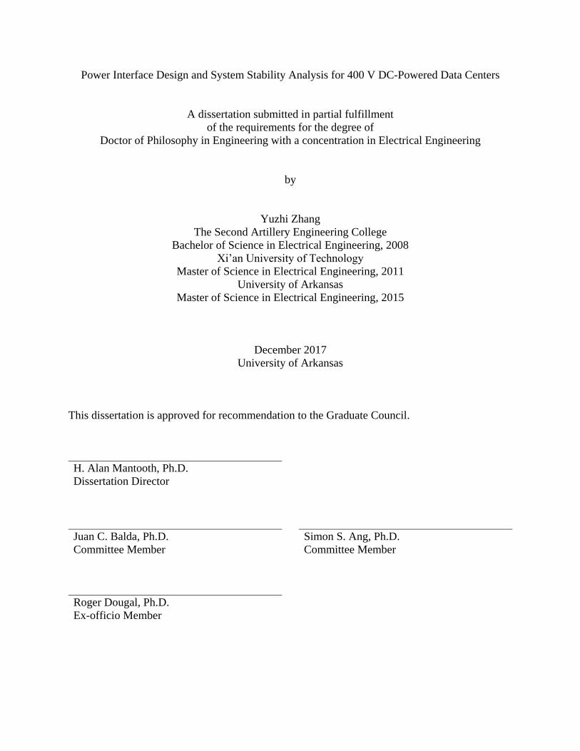
This dissertation is approved for recommendation to the Graduate Council.
H. Alan Mantooth, Ph.D.
Dissertation Director
Juan C. Balda, Ph.D.
Committee Member
Simon S. Ang, Ph.D.
Committee Member
Roger Dougal, Ph.D.
Ex-officio Member

ABSTRACT
The demands of high performance cloud computation and internet services have increased in
recent decades. These demands have driven the expansion of existing data centers and the
construction of new data centers. The high costs of data center downtime are pushing designers to
provide high reliability power supplies. Thus, there are significant research questions and
challenges to design efficient and environmentally friendly data centers with address increasing
energy prices and distributed energy developments.
This dissertation work aims to study and investigate the suitable technologies of power
interface and system level configuration for high efficiency and reliable data centers.
A 400 V DC-powered data center integrated with solar power and hybrid energy storage is
proposed to reduce the power loss and cable cost in data centers. A cascaded totem-pole bridgeless
PFC converter to convert grid ac voltage to the 400 V dc voltage is proposed in this work. Three
main control strategies are developed for the power converters. First, a model predictive control is
developed for the cascaded totem-pole bridgeless PFC converter. This control provides stable
transient performance and high power efficiency. Second, a power loss model based dual-phase-
shift control is applied for the efficiency improvement of dual-active bridge converter. Third, an
optimized maximum power point tracking (MPPT) control for solar power and a hybrid energy
storage unit (HESU) control are given in this research work. The HESU consists of battery and
ultracapacitor packs. The ultracapacitor can improve the battery lifetime and reduce any transients
affecting grid side operation.
The large signal model of a typical solar power integrated datacenter is built to analyze the
system stability with various conditions. The MATLAB/Simulink™-based simulations are used

to identify the stable region of the data center power supply. This can help to analyze the sensitivity
of the circuit parameters, which include the cable inductance, resistance, and dc bus capacitance.
This work analyzes the system dynamic response under different operating conditions to determine
the stability of the dc bus voltage. The system stability under different percentages of solar power
and hybrid energy storage integrated in the data center are also investigated.

© 2017 Yuzhi Zhang
All Rights Reserved

ACKNOWLEDGMENTS
First and foremost, I would like to express my sincere appreciation to my advisor, Prof. H.
Alan Mantooth, who inspires my study, work, and life so much with his insightful vision, broad
knowledge, professionalism, and creative thinking. I benefit a lot from Prof. Mantooth not only in
many good projects but also his great personalities and leadership. I really enjoyed my five years
of study and work with Prof. Mantooth’s guidance and mentorship. He will be an inspiring role
model for my future career growth.
I am very grateful to my other committee members, Prof. Juan C. Balda, Prof. Simon S. Ang,
and Prof. Roger Dougal for their technical assistance, valuable suggestions and helpful discussion
during my Ph.D. study. I’d like to offer my special thanks to Prof. Balda for his technical support,
time and encouragement for my Ph.D. project. I’d also like thank Prof. Ang for his help for my
Little Box Challenge project. I want to thank Prof. Dougal, at the University of South Carolina,
for his help regarding my projects in the GRAPES NSF research center.
I am thankful to all my colleagues with whom I have worked together on many interesting
projects. I’d like to thank Chris Farnell and Sayan Seal in regard to the Arkansas Powerbox project.
I also appreciate the help from my other professors, colleagues, and friends: Prof. Yue Zhao, Prof.
Roy A. McCann, Prof. Shui-Qing (Fisher) Yu, Prof. Randy Brown, Mrs. Connie Howard, Dr. Tao
Yang, Haoyan Liu, Janviere Umuhoza, Joe Moquin, Tavis Clemmer, Shuang Zhao, Audrey
Dearien, Ramchandra Kotecha, Nan Zhu, Yusi Liu and Fahad Hossain. I’d also like to thank Dr.
Liang Jia, Udaya Kiran Ammu, and Neilus O'Sullivan for their help and guidance during my
internship at Google’s Mountain View office.

I’d like to thank Shan Xu for supporting me through days and nights spent accomplishing my
research work and making my Ph.D. study a happy journey.
Finally, and most importantly, I am extremely grateful to the University of Arkansas for
supporting me during my Ph.D. Study.

DEDICATION
This dissertation is dedicated to my parents, Naizhu Zhang and Xiange Guo. My heartfelt
gratitude goes to them for their everlasting love, strength and support through my entire life. This
dissertation is also dedicated to my brother, Yuhua Zhang and my sisters, Qingxiu Zhang, Qingmei
Zhang, Guiqing Zheng, Xinhua Zhang.

TABLE OF CONTENTS
CHAPTER 1 INTRODUCTION AND THEORETICAL BACKGROUND ........................... 1
1.1 Background: The Challenge and Opportunity of Data Center Power Conversion ... 1
1.1.1 Quantity and capacity expansion of data centers .................................................. 1
1.1.2 Climbing electricity price ...................................................................................... 2
1.1.3 High cost of data center power supply downtime ................................................. 3
1.2 Previous Research ..................................................................................................... 4
1.2.1 Power distribution bus: 120 VAC or 400 VDC .................................................... 4
1.2.2 Integration with renewable energy and stability consideration ............................. 5
1.2.3 Energy storage in data center ................................................................................ 6
1.3 Proposed 400 V DC-powered Data Center with Solar Power Integration ................ 8
1.4 Problem Definitions ................................................................................................ 10
1.4.1 Topology consideration ....................................................................................... 10
1.4.2 Controller consideration: Proportional-Integral Control vs Model Predictive
Control 11
1.4.3 Efficiency consideration ...................................................................................... 12
1.4.4 Green data center ................................................................................................. 14
1.5 Outline..................................................................................................................... 14
1.6 Reference ................................................................................................................ 16
CHAPTER 2 DESIGN, MODELING AND CONTROL OF RECTIFIER STAGE .............. 17
2.1 Introduction and Motivation ................................................................................... 17
2.1.1 Ac/dc voltage conversion with low-frequency transformer ................................ 17
2.1.2 Ac/dc voltage conversion with high-frequency transformer ............................... 21
2.1.3 Design of cascaded scaled-down totem-pole multilevel converter ..................... 33
2.2 Control Strategy: PI Control vs Model Predictive Control ..................................... 35
2.2.1 Conventional PI control ...................................................................................... 35
2.2.2 Conventional PI controller design steps for a boost converter ............................ 37
2.2.3 Model predictive control ..................................................................................... 40
2.2.4 Discretization method: from continuous-time domain to discrete-time domain . 40
2.2.5 Comparison of PI and MPC ................................................................................ 44
2.3 MPC design for Cascaded Bridgeless Totem-Pole Multilevel Converter .............. 45
2.3.1 Cascaded totem-pole converter modeling ........................................................... 46

2.3.2 Cost function of totem-pole converter ................................................................ 48
2.3.3 Block diagram of controllers ............................................................................... 53
2.3.4 Simulation and experiment verification .............................................................. 54
2.4 Conclusion .............................................................................................................. 58
2.5 Reference ................................................................................................................ 60
CHAPTER 3 MODELING AND CONTROL OF SOLID STATE TRANSFORMER DC/DC
STAGE: EFFICIENCY IMPROVEMENT .................................................................................. 63
3.1 Introduction and Motivation ................................................................................... 63
3.2 Dual Active Bridge Operation ................................................................................ 65
3.2.1 Single phase-shift control .................................................................................... 65
3.2.2 Extended phase-shift control ............................................................................... 66
3.2.3 Dual-phase-shift control ...................................................................................... 67
3.2.4 Triple phase-shift control .................................................................................... 68
3.2.5 Conclusion ........................................................................................................... 70
3.3 Efficiency Optimization Methods ........................................................................... 70
3.3.1 Current stress minimization method ................................................................... 70
3.3.2 Circulating power reduction method ................................................................... 73
3.4 SiC MOSFET-based DAB Operation Principle ..................................................... 74
3.5 Simplified Power Loss Model and Improved Power Loss Model .......................... 80
3.5.1 Switching loss analysis and modeling ................................................................. 80
3.5.2 Conduction loss analysis and modeling .............................................................. 82
3.5.3 The power loss from the transform and auxiliary inductor ................................. 83
3.6 The Total Loss Model ............................................................................................. 85
3.7 Efficiency Optimized Method: Lagrangian Objective Function ............................ 85
3.7.1 Power delivery capability .................................................................................... 85
3.7.2 Minimum power loss design ............................................................................... 87
3.7.3 Control strategy of DAB with loss model ........................................................... 88
3.8 Experimental Verification ....................................................................................... 88
3.8.1 Same Vout_ref and same load power, different Vin ................................................ 89
3.8.2 Same Vin, different load power ........................................................................... 90
3.9 Loss Model Based Efficiency Improvement Conclusion ....................................... 90
3.10 Transient Performance Improvement Methods ...................................................... 91
3.10.1 Introduction ......................................................................................................... 91
3.10.2 Proposed K-Factor control with the virtual capacitor for a DAB ....................... 94
3.10.3 Comparative analysis of transit response characterization ............................... 106

3.10.4 Hardware experimental validation of the proposed control .............................. 114
3.10.5 Conclusion of virtual capacitor based K-factor control .................................... 117
3.11 Other Testing Results ............................................................................................ 117
3.12 Reference .............................................................................................................. 121
CHAPTER 4 DISTRIBUTED ENERGY INTEGRATION AND HYBRID ENERGY
MANAGEMENT STRATEGY FOR 400 V DATA CENTER ................................................. 126
4.1 Introduction and Motivation ................................................................................. 126
4.2 Description of Green Data Center ......................................................................... 127
4.3 PV Topology and MPPT Control ......................................................................... 128
4.4 PV Power Spectrum Analysis ............................................................................... 133
4.5 Hybrid Energy Storage ......................................................................................... 134
4.5.1 Controller design of the buck/boost converter for the battery and ultracapacitor
packs 135
4.5.2 Power reference calculation .............................................................................. 136
4.6 Grid-Side Converter Design ................................................................................. 137
4.7 Case Study and Simulation Verification ............................................................... 139
4.7.1 Data center integrated with solar power and hybrid energy storage ................. 139
4.7.2 Different percentages of solar power in data center .......................................... 143
4.8 Conclusion ............................................................................................................ 146
4.9 Reference .............................................................................................................. 148
CHAPTER 5 SYSTEM LEVEL STABILITY ANALYSIS FOR 400 V DATA CENTER 150
5.1 Stability Issue in a Data Center ............................................................................. 150
5.2 Mathematical Model: Large Signal Modeling of Large-Scale Data Center ......... 150
5.3 Stability Criterion Introduction ............................................................................. 152
5.4 Simulation Results and Stability Analysis ............................................................ 154
5.5 Conclusion ............................................................................................................ 156
5.6 References ............................................................................................................. 157
CHAPTER 6 CONCLUSION FUTURE WORK ................................................................. 158
6.1 Conclusion ............................................................................................................ 158
6.2 Future work ........................................................................................................... 159

LIST OF FIGURES
Fig. 1-1 Total Electricity Consumption of Data Centers in U.S. [1.1] ..................................... 2
Fig. 1-2 Annual Average Retail Price of Electricity [1.2] ........................................................ 3
Fig. 1-3 Traditional ac Distribution Efficiency......................................................................... 4
Fig. 1-4 Efficiency of 400 V DC Distribution Architecture ..................................................... 5
Fig. 1-5 Cable Size Comparison between 48 V and 400 V with 100 kW Load ....................... 5
Fig. 1-6 Ultracapacitor Consumption by Market [1.5] ............................................................. 7
Fig. 1-7 Ultracapacitor Module from Schneider [1.5] .............................................................. 7
Fig. 1-8 Conventional AC-powered Data Center ..................................................................... 9
Fig. 1-9 400 V DC-powered Data Center Integrated with Solar Power and Energy Storage ... 9
Fig. 1-10 A Typical Power Losses in a Data Center [1.3] ...................................................... 13
Fig. 2-1 Ac/dc Power Conversion: with Low-Frequency Transformer Application .............. 17
Fig. 2-2 Classic Boost-type Rectifier ...................................................................................... 18
Fig. 2-3 Totem-pole Bridgeless PFCs with Wide Bandgap Devices ...................................... 19
Fig. 2-4 Simulation Results of Efficiency Comparison: 240 V ac to 400 V dc with 5 kW Load
....................................................................................................................................................... 20
Fig. 2-5 System Configuration Using Medium- or High-frequency Transformer .................. 21
Fig. 2-6 Five-level NPC ac/dc Topology ................................................................................ 22
Fig. 2-7 Modular Multilevel PFC Converters ......................................................................... 24
Fig. 2-8 Multi-Cell Boost Topology with Four Input Series Output Parallel Connected
Converter....................................................................................................................................... 25
Fig. 2-9 Proposed Topology for 1 MW Power Data Center ................................................... 27
Fig. 2-10 Proposed Topology for 10 MW Power Data Center ............................................... 31

Fig. 2-11 Proposed Topology for 30 MW Power Data Center ............................................... 32
Fig. 2-12 Totem-pole Bridgeless PFC Converter, Two Cells ................................................. 33
Fig. 2-13 Boost Converter Topology as Example .................................................................. 36
Fig. 2-14 Equivalent Circuits with Switch On and Off .......................................................... 37
Fig. 2-15 Bode-plot of a Boost Converter in PLECS ............................................................. 39
Fig. 2-16 The Procedure to Choose the Proper Switching State ............................................. 43
Fig. 2-17 Design Flowcharts of PI and MPC Control ............................................................ 44
Fig. 2-18 Scaled-down Prototype: ac/dc Stage, Two Cells .................................................... 45
Fig. 2-19 Simulation Results of 400 dc Bus Balance Performance ........................................ 50
Fig. 2-20 The Flowchart of MPC ........................................................................................... 53
Fig. 2-21 The Block Diagram of MPC and Conventional PI for the Proposed Topology ..... 54
Fig. 2-22 Normal Operation to Step-up Load of the Two Controllers ................................... 55
Fig. 2-23 Gate Signals For a Selected Switch Position For Conventional PI Control............ 56
Fig. 2-24 Gate Signals for a Selected Switch Position for Model Predictive Control ............ 56
Fig. 2-25 Experimental Setup: Typhoon Simulator and DSP Control Card ........................... 57
Fig. 2-26 Hardware-In-Loop Testing Results of Conventional PI Control (Time: 25 ms/div,
vo1=vo2=400 V, iload: 0 to 12.5 A) ................................................................................................... 58
Fig. 2-27 Hardware-In-Loop Testing Results of The Proposed Model Predictive Control (Time:
25 ms/div, vo1=vo2=400 V, iload: 0 to 12.5 A) ................................................................................. 58
Fig. 3-1 Dual-Active Bridge with Single Phase-Shift Control ............................................... 65
Fig. 3-2 Single Phase-Shift Control: The Transformer Input/Output Voltage and Inductor Lk
Current .......................................................................................................................................... 66
Fig. 3-3 Dual-Active Bridge with Extended Phase-Shift Control .......................................... 67

Fig. 3-4 Extended Phase-Shift Control: The Transformer Input/Output Voltage and Inductor
Lk Current ...................................................................................................................................... 67
Fig. 3-5 Dual-Active Bridge with Dual Phase-Shift Control .................................................. 68
Fig. 3-6 Dual Phase-Shift Control: The Transformer Input/Output Voltage and Inductor Lk
Current .......................................................................................................................................... 68
Fig. 3-7 Dual-Active Bridge with Triple Phase-Shift Control ................................................ 69
Fig. 3-8 Triple Phase-Shift Control: The Transformer Input/Output Voltage and Inductor Lk
Current .......................................................................................................................................... 69
Fig. 3-9 Control Diagram of Current Stress Minimization ..................................................... 71
Fig. 3-10 Control Diagram of Circulating Power Reduction .................................................. 74
Fig. 3-11 Control Signal and Circuits Waveform when Di<Do .............................................. 75
Fig. 3-12 10 Operational Stages when Di<Do ......................................................................... 76
Fig. 3-13 Power Curve of the DAB with Dual-Phase-Shift Control ...................................... 86
Fig. 3-14 Power Loss 3D Plot when DAB with Dual-Phase-Shift Control ............................ 86
Fig. 3-15 Control Diagram of Power Loss Minimization ....................................................... 88
Fig. 3-16 Efficiency Testing Results of SPS, Accurate Model and Simple Model with Vary
Input Voltage ................................................................................................................................ 89
Fig. 3-17 Efficiency Testing Results of SPS, Accurate Model and Simple Model with Varying
Load Power ................................................................................................................................... 90
Fig. 3-18 DAB Converter with Phase-Shift Control ............................................................... 95
Fig. 3-19 Transformer Primary and Secondary Voltages, DAB Inductor Current with DPS
Control .......................................................................................................................................... 96
Fig. 3-20 Bode plot of Type I K-factor controller ................................................................ 101

Fig. 3-21 Bode Plot of K-factor Type II Control .................................................................. 102
Fig. 3-22 Bode Plot of K-factor Type III Control ................................................................. 103
Fig. 3-23 DAB System with Virtual Capacitor ..................................................................... 105
Fig. 3-24 Control Diagram of Power Loss Minimization ..................................................... 106
Fig. 3-25 Bode plot of DAB with Different Controllers ....................................................... 109
Fig. 3-26 Step-up Load, Output Voltage Transit with Virtual Capacitor ............................. 110
Fig. 3-27 Step-down Loads Response for Three Controllers ............................................... 112
Fig. 3-28 Step-up Loads Response for Three Controllers .................................................... 113
Fig. 3-29 The Scaled-down Prototype of DAB .................................................................... 114
Fig. 3-30 Comparison betweed the output power in closed-loop avergae model and
experimental results .................................................................................................................... 115
Fig. 3-31 Transient Reponse with Step Load Results With PI, K-factor, and K+VC ......... 116
Fig. 3-32 The Scaled Down Prototype of Overall System .................................................... 118
Fig. 3-33 Yellow: Grid voltage vgrid= 240 VAC, Blue: Grid current igrid= 2.1 A, Purple: DAB
primary side dc voltage vin=200 VDC ........................................................................................ 119
Fig. 3-34 Testing results of DAB with SPS control.............................................................. 119
Fig. 3-35 Testing results of DAB with Loss Model Based-DPS control .............................. 120
Fig. 4-1 Generic Configuration of A 400 V DC-Powered Data Center Integrated With Solar
Power and Energy Storage Units ................................................................................................ 128
Fig. 4-2 Circuit Diagram of the Considered PV Farm .......................................................... 130
Fig. 4-3 Flowchart for the Calculation of the Duty Cycle of the Boost Converter ............... 131
Fig. 4-4 PV Simulation Results with Constant and Variable Duty Cycle Step-Size P&O MPPT
Methods....................................................................................................................................... 133

Fig. 4-5 Frequency Spectrum Analysis of PV Power Over A 24-Hour Period .................... 134
Fig. 4-6 Circuit Diagram of the Energy Storage Packs ........................................................ 135
Fig. 4-7 Control Diagram of the Battery Pack ...................................................................... 136
Fig. 4-8 Control Diagram of the Ultracapacitor Pack ........................................................... 136
Fig. 4-9 Power Reference Generation for Battery and Ultracapacitor .................................. 137
Fig. 4-10 Block Diagram of the Grid-Side Converter .......................................................... 138
Fig. 4-11 The Control Algorithm of the Grid-side Converter .............................................. 138
Fig. 4-12 Control Strategy of PLL ........................................................................................ 139
Fig. 4-13 Solar Irradiance on a Cloudy Day ......................................................................... 139
Fig. 4-14 Solar Irradiance on a Rainy Day ........................................................................... 140
Fig. 4-15 Solar Irradiance on an Overcast Day..................................................................... 140
Fig. 4-16 Solar Irradiance on a Clear Day ............................................................................ 140
Fig. 4-17 Rack Power and PV Power on a Cloudy Day Over 24 Hours .............................. 141
Fig. 4-18 Power Flows of the Grid and Battery without Ultracapacitor Pack ...................... 141
Fig. 4-19 Power Flows of the Grid and Battery with Ultracapacitor Pack ........................... 142
Fig. 4-20 The 400-V DC Bus Voltage without Ultracapacitor Compensation ..................... 143
Fig. 4-21 The 400-V DC Bus Voltage and Ultracapacitor Powers with Ultracapacitor
Compensation ............................................................................................................................. 143
Fig. 4-22 DC Bus Voltage Performance of 0.5 MW, 1.5 MW, and 3 MW Data Center with
Solar Power ................................................................................................................................. 146
Fig. 5-1 Large Signal Model of 400 V DC-Powered Data Center ........................................ 151
Fig. 5-2 The Specification of Pole Location [5.6] ................................................................ 153
Fig. 5-3 System Stability: Eigenvalue and Voltage Response .............................................. 153

Fig. 5-4 Stable Boundary of Different dc Bus Cable Impedance ......................................... 155
Fig. 5-5 Stable Boundary of DC Bus Capacitor. 200μF: 0.2 ms (Green), 0.15 ms (Orange), 0.1
ms (Blue), 0.05 ms (Red). 2000μF: 0.2 ms (Green), 0.15 ms (Orange), 0.1 ms (Blue), 0.05 ms (Red)
..................................................................................................................................................... 156

LIST OF TABLES
Table 2.1 Comparison of Three Typical PFC Converters ...................................................... 20
Table 2.2 Switch Specification in 1 MW Data Center ............................................................ 28
Table 2.3 Switch Specification in 10 MW Data Center .......................................................... 31
Table 2.4 Switch Specification in the Scaled-down ac/dc Converter ..................................... 34
Table 2.5 Switching Cases of Cascaded Bridgeless Totem-pole PFC .................................... 51
Table 3.1 The Inductor Lk Current Equations, Di<Do ............................................................. 77
Table 3.2 The Switching Actions in One Switching Period ................................................... 79
Table 3.3 The Conduction Actions in One Switching Period ................................................. 79
Table 3.4 Parameters for Simulation .................................................................................... 107
Table 3.5 Circuit Parameters for the Scaled Down Prototype .............................................. 118
Table 4.1 The PV Panels Simulation Parameters ................................................................. 132
Table 4.2 DC Bus Ripple of 0.5 MW Data Center with Variable Solar Power .................... 144
Table 4.3 DC Bus Ripple of 1.5 MW Data Center with Variable Solar Power .................... 144
Table 4.4 DC Bus Ripple of 3 MW Data Center with Variable Solar Power ....................... 145
Table 5.1 Simulation Parameters .......................................................................................... 154

1
CHAPTER 1
INTRODUCTION AND THEORETICAL BACKGROUND
1.1 Background: The Challenge and Opportunity of Data Center Power Conversion
1.1.1 Quantity and capacity expansion of data centers
The popularity of internet services and cloud computing is leading to continuous expansion of
data centers. To meet the demands of high computation speed and data storage capacity, the
quantity and capacity of data centers is rapidly increasing. Larger IT companies such as Microsoft,
Google, Facebook, Alibaba, and Baidu are building more data centers around the world. At the
same time, the energy required by data centers is climbing very quickly. The Lawrence Berkeley
National Laboratory, in collaboration with experts at Stanford, Carnegie Mellon, and Northwestern
published a figure showing the rising energy consumption by data centers, which is given in Fig.
1-1 [1.1]. In 2013, the electricity used by data centers increased to 70 billion kilowatt-hours (kWh).
The amount of 70 billion kWh is close to 1.8% of total electricity usage in the U.S. in 2014. The
report shows the electricity consumption is expected to continue increasing to up to 4% of total
electricity usage of the U.S. by 2020.

2
Fig. 1-1 Total Electricity Consumption of Data Centers in U.S. [1.1]
1.1.2 Climbing electricity price
From the electricity data provided by the U.S. Energy Information Administration, illustrated
in Fig. 1-2 [1.2], the energy prices are climbing every year. From 2001 to 2014, the average retail
price of industrial electricity increased from 5.05 cents per kWh to 7.1 cents per kWh. For example,
the actual monthly critical average power of a 10 MW data center often is 4-6 MW [1.3]. The
monthly average power is selected as 5 MW. The industrial electricity price is 7.1 cents per kWh.
If the power converter reaches 5% power loss reduction, then the electricity cost reduction will be
$155,098 per data center per year, and the related cost will also be further reduced, like the costs
of operational and cooling systems.

3
Fig. 1-2 Annual Average Retail Price of Electricity [1.2]
The efficiency is the key element to reduce the total power consumption, increase the power
density and lead to small footprint of data centers. The design of high efficiency data centers
includes power transmission, conversion, and distribution development.
1.1.3 High cost of data center power supply downtime
Due to the power capacity and expansion of data centers, the reliability of data centers is
becoming increasingly important. Due to the growing quantity and density of data centers, the
consequences of outages are increasing. Emerson Company reports, data centers have an average
downtime of 2.34 hours, and an average of 2.5 outages per year [1.4]. For 500,000 data centers,
the Emerson Company estimated $2.84 million in annual outage costs for data centers. Designing
a more reliable power supply would reduce expensive downtime and avoid associated costs.
To meet the requirements of high performance and low power loss, many researchers have
been working on power topology development, integration with renewable energy, system level
stability analysis, etc. The detailed research status is summarized in the following section.

4
1.2 Previous Research
1.2.1 Power distribution bus: 120 VAC or 400 VDC
The typical efficiencies obtainable through the ac system technologies in data centers are given
in Fig. 1-3. A traditional Uninterruptible Power Supply (UPS) architecture is utilized. It employs
at least two stages. Ac voltage from the grid side is converted to dc voltage first. An energy storage
device, like lead-acid batteries, is connected to the dc bus. The dc bus is then inverted to an ac bus
which is the Power Distribution Unit (PDU). The advantage of this traditional four stages
architecture is robustness. However, the end-to-end efficiency is a relatively low 71%. From article
[1.3], about 15% of data center’s power is wasted and dissipated as heat.
Fig. 1-3 Traditional ac Distribution Efficiency
Dc distribution is attractive, it eliminates at least one power inversion stage, resulting in higher
efficiency. The efficiency performance of dc distribution is shown in Fig. 1-4. Compared with the
ac distribution, the efficiency is improved from 71% to 90%. This 19% efficiency increase leads
to significant cost reduction of the cooling system. What’s more, as the power distribution voltage
is increased to 400 V dc, the conduction loss can be reduced, allowing the use of lighter and more
economic cables. The power cable comparison between 48 V dc and 400 V dc is shown in Fig.
1-5.
Server
AC/DC DC/ACUtility Line
Voltage
480 V3fAC
96% x 97% x 90% x 86% = 71%
PDU120 V1f
AC
PSU
AC/DC DC/DC
12 V
Ele
ctro
nic
Lo
ad
s
VR
VR
Fans

5
Fig. 1-4 Efficiency of 400 V DC Distribution Architecture
Fig. 1-5 Cable Size Comparison between 48 V and 400 V with 100 kW Load
Another merit of the dc distribution architecture is its ease in integrating with distributed
energy sources, such as solar photovoltaic, wind turbine, fuel cell, etc. In current commercial
technologies, dc equipment is available, but the costs are higher than comparable ac equipment.
In this dissertation, a 400 V bus is selected due to higher efficiency consideration. The power
topology development and design is analyzed and designed in detail in Chapters 2 to 5.
1.2.2 Integration with renewable energy and stability consideration
Usually, data centers are built in a place with reliable and sustainable sources of power;
protected from hazards, environment friendly and so on. Unfortunately, those places are not the
best choice for renewable energy generation where the data center has better efficiency
Utility Line
Voltage
480 V3fAC
400 Vdc 400 Vdc
Server
PSU
DC/DC12 V
Ele
ctro
nic
Lo
ad
s
VR
VR
Fans
DC/DC48 V
99% x 99% x 99% x 99% x 94% = 90%
AC-DC Converter
PDU

6
performance. What’s more, data center operation needs reliable power, but solar power is only
available during the daytime and wind power is only available when the wind is blowing. The truth
of the ‘Green Data Center’ mentioned from the industrial side is that these companies purchase at
least an equivalent amount of power from renewable energy companies and sell the energy back
into the grid at a wholesale price [1.3]. Given the large size of many data centers, the large roofs
offer excellent real estate for solar panel placement. This dissertation considers solar panels on
the roof as green power and utilizes energy storage to reduce the electricity cost and the non-green
emissions from the grid. Due to the randomness and fluctuation of solar power generation, the
effects to the system stability will be investigated in this dissertation.
1.2.3 Energy storage in data center
Energy storage, such as batteries, play an important role in the UPS system. It supplies the
uninterrupted power to critical loads. Power transients, due to solar irradiance transients or load
changes, need to be smoothed by the energy storage. Lead-acid batteries are widely used in the
data center due to their low cost. However, rapid charging and discharging degrade the life
expectancy of a battery pack. To overcome this drawback, ultracapacitor packs are considered in
this work. The ultracapacitor application market is shown in Fig. 1-6 [1.5]. The global
ultracapacitor consumption is fast growing. This market is expected to grow from $500M in 2015
to $1.5B around 2020. One type of ultracapacitor module from Schneider is shown in Fig. 1-7.
With more technological advancements, both the cost and maintenance of ultracapacitors have
gone down.

7
Fig. 1-6 Ultracapacitor Consumption by Market [1.5]
Fig. 1-7 Ultracapacitor Module from Schneider [1.5]
Ultracapacitors allow more charge/discharge cycles and have a higher power density, which
are desirable for fast power smoothing. In this dissertation, an investigation is conducted for the
design of high frequency ripple reduction and battery lifetime improvment, which are both
compensated by ultracapacitors.

8
1.3 Proposed 400 V DC-powered Data Center with Solar Power Integration
As mentioned, the traditional ac bus data center configured as shown in Fig. 1-8 has low
efficiency in the distribution unit. For high efficiencies and high power densities, high-power dc
distribution, such as 400 V in DC-powered data centers, is becoming more attractive. Due to the
high power levels of data centers, the input of the ac/dc converter is usually connected to a
medium-voltage power grid through bulky low-frequency step-up transformers. Recently, high-
frequency transformers in multilevel converters are investigated due to their small size, light
weight, high power density and capability for integrating multiple functions [1.6][1.7]. The
proposed 400 V DC-powered data center is shown in Fig. 1-9. Compared with traditional ac bus
data centers, the low-frequency transformer is replaced by a solid-state transformer and the power
distribution is improved with a higher voltage 400 V bus, thus the current in the bus bars are
decreased. The conduction power loss and cable cost in the distribution bus bars are reduced as
well. To reduce the voltage stresses on switches and increase the current carrying capabilities,
different multilevel converter topologies have been investigated by various groups [1.8][1.9].
Some topologies utilize high breakdown voltage IGBTs. However, IGBTs are inherently slow
devices and have a tail current. The tens of kV power MOSFETs are rarely available in the market
and mostly under investigation in the research environment. For high efficiency and switching
speed considerations, commercial SiC power MOSFETs rated from 0.9 kV to 1.7 kV are adopted
in this paper.

9
Fig. 1-8 Conventional AC-powered Data Center
Fig. 1-9 400 V DC-powered Data Center Integrated with Solar Power and Energy Storage
kVAC
120/240
VAC
Grid 2
Grid 1
Diesel Generators
S3
S2
S1
PV Array Wind Farm
Critical Fans and Lighting
Transmission line
Green Energy
Room AC
LF Transformer
S4 Hard drives
Fan
CPU
Memory
48VDC
RACK 1
Battery I1
Hard drives
Fan
CPU
Memory
48VDC
RACK n
Battery I2
AC Bus
400VDC
Grid 2
Grid 1
Diesel Generators
S3
S2
S1
PV Array Wind Farm
Critical Fans and Lighting
Transmission line
Green
Energy
Room AC
SST Structure
S4 Hard drives
Fan
CPU
Memory
48VDC
RACK 1
Battery I1
Hard drives
Fan
CPU
Memory
48VDC
RACK n
Battery In
Battery II
Ultracaps
Solar Panels

10
Furthermore, to build a real ‘green’ data center and reduce the energy consumption from grid
side, in the evaluated system the locally produced solar power is interfaced to the 400 V dc bus
through dc/dc converters. To maintain the 400 V dc bus, the battery and ultracapacitor packs are
interfaced with the same 400 V dc bus through dc/dc converters. A high-power active-front-end
rectifier is utilized at the grid side. The existing 48 V telecom power supply is recognized as a
more economical and practical option. To minimize the revision from the existing power supply
in data center, 48-V dc bus is kept in the rack. The battery as back-up energy is on the 48-V dc bus
as well. A dc/dc converter steps down 400 V to 48 V in the server racks.
1.4 Problem Definitions
There are many research topics in a data center. The high reliability, efficiency and green data
center are identified as the main topics in this dissertation.
1.4.1 Topology consideration
1.4.1.1 The issue in ac/dc voltage conversion
For ac/dc voltage conversion, Power Factor Correction (PFC) converters are widely adopted.
The most popular and conventional PFC converter is the diode bridge rectifier in series with a
boost converter. The benefit of this topology is that just one switch needs to be controlled. The
drawback is that at least two diodes are on in every power delivery circle, leading to inefficient
power conversion. Some soft-switching controllers are investigated to reduce the reverse recovery
of Si diodes [1.10][1.11]. Complicated auxiliary circuits and more complex controls are needed to
realize soft-switching.

11
1.4.1.2 Proposed solution for ac/dc voltage conversion
In this dissertation, two different types of bridgeless PFC converters are carefully compared
with the diode full bridge rectifier. The dual boost bridgeless PFC (DBP) converter has better
efficiency performance by reducing the conduction loss on the diodes. It requires more
components, which means the need of auxiliary gate drivers and higher cost. Two high frequency
diodes are required in the DBP converter.
Another bridgeless PFC converter is the totem-pole bridgeless PFC (TPBP) converter. The
challenge of TPBP converter is that it usually works in discontinuous-current mode (DCM) or
critical-current mode (CRM) due to efficiency consideration. The poor reverse recovery time of
MOSFETs are reduced in SiC MOSFETs and the on-state resistance of SiC MOSFETs are also
less than the Si MOSFET. These two features allow the TPBP converter to work in continuous-
current mode (CCM) with much greater efficiency. The TPBP converter has the lowest volume of
components. If the two diodes in the TPBP converter are switched at ac voltage frequency, then
the power loss is further reduced.
1.4.2 Controller consideration: Proportional-Integral Control vs Model Predictive
Control
1.4.2.1 The issue in controller design for load or voltage transient
In the power supply design of power converters for data center applications, the transient
response capability is the key requirement. The conventional proportional-integral (PI) control is
very popular in the area of power converter controller design. Usually, it has two loops: voltage
loop and current loop. The challenge in regarding PI controllers is that different load power or
voltage transient needs different phase and gain compensation, thus the controller design varies

12
from light load to heavy load. What’s more, the controller complexity is increased if compensating
for the aforementioned load variances.
1.4.2.2 Proposed solution for transient performance
To overcome these disadvantages, a model predictive control (MPC) is proposed in this
dissertation. MPC is a real time control algorithm. It predicts the expected control variable and
determines the optimized control period. The mathematical model of the controlled converter is
utilized in MPC control. Different from the conventional PI control, the frequency of MPC control
is variable which is dependent on the feedback. However, the maximum frequency can be less or
equal to the conventional PI control, thus MPC can improve the efficiency. Another merit of MPC
is that the multi-goal control can be realized. The coefficient of different goals need to be
investigated.
1.4.3 Efficiency consideration
1.4.3.1 Issue in power conversion efficiency
The typical total energy usage of a conventional datacenter includes the IT equipment, cooling
system, uninterrupted power supply (UPS), power distribution, and ancillary systems. The detailed
percentages of different power consumption is given in Fig. 1-10. The power usage effectiveness
(PUE) presents the ratio of IT power to the total power, which reflects the efficiency of a datacenter
infrastructure. The IT power is the power consumed by the servers. The power converter is the key
factor to improve the power efficiency, thus guaranteeing lower PUE. Many researches have been
working on the efficiency improvement in power converters in the data center, such as
development of new power topology, soft switching, control strategy, etc. For example, there are
two popular efficiency improvement methods for the isolated dc/dc power converter known as the

13
dual-active bridge (DAB). The first method is a current stress optimizing algorithm and the second
is a flow-back power minimization strategy. The DAB is used in final stage of the proposed
topology in this work.
Fig. 1-10 A Typical Power Losses in a Data Center [1.3]
1.4.3.2 Proposed solution for efficiency improvement
In this dissertation, the improvement of the efficiency performance in a dual-active bridge for
the data center power supply is discussed. Different from the reported methods, an accurate loss
model is developed in this work for the power converter to find the expected phase-shift angle for
the switches. The accurate loss model method is developed from three aspects which are the
conduction loss model, switching loss model, and a high frequency transformer loss model. The
better loss model leads to the more accurate prediction of phase-shift in the dual-active bridge, and
thus smaller losses.

14
1.4.4 Green data center
1.4.4.1 Issue in current ‘green’ data centers
The integration of solar power and data centers can highly reduce the electricity cost and
emissions of data centers. However, solar power is not stable and heavily depends on the
environment. Battery energy storage has relatively high energy density. It is usually utilized to
smooth the power output from solar systems. However, the lifetime of batteries is a major issue,
leading to cost increases.
1.4.4.2 Proposed solution for ac/dc voltage conversion
The ultracapacitor has a high power density and can be quickly charged and discharged without
harming its lifetime. In this dissertation, the battery and ultracapacitor are used as hybrid energy
storage devices to smooth the solar power. The controller design for each energy storage device is
developed as well to achieve high performance.
1.5 Outline
Chapter 2 describes the rectifier power stage and the control strategies for the cascaded totem
-pole PFC converter. The conventional PI control design and the proposed model predictive
control are developed, analyzed and compared. A discrete time mode of a cascaded totem-pole
PFC converter is derived and utilized to design the model predictive control. The control goals
include unity power factor, dc bus voltage balance, power loss minimization, etc.
Chapter 3 illustrates the dc/dc stage in the proposed topology. The operation principle of a
dual-active bridge converter is analyzed. The single and dual phase-shift control is compared. To
improve the efficiency performance, the backflow power reduction and current stress minimization
methods are given. The loss model optimization method is proposed to achieve better efficiency

15
performance. Simulation and testing results are given to verify the proposed control strategy. For
the control of transient performance, the conventional PI control and proposed K-factor control
are designed and compared. A scaled-down prototype is tested to verify the proposed K-factor
control.
Chapter 4 is about the solar power and hybrid energy storage integration in the data center. The
controllers for solar power, battery, ultracapacitor and data center loads are developed. The
simulation results are given to validate the effectiveness of the proposed topology and its control
strategies.
Chapter 5 shows the system level stability analysis of a data center. The large signal model of
a large-scale data center is built. The stability criterion is introduced and the stable region is given
through the MATLAB/SimulinkTM simulation results.
Chapter 6 is the summary of this dissertation and the outlook of the future work.

16
1.6 Reference
[1.1] “United States Data Center Energy Usage Report.” [Online]. Available:
https://eta.lbl.gov/publications/united-states-data-center-energy.
[1.2] “U.S. Electric System Operating Data.” [Online]. Available:
http://www.eia.gov/electricity/data.cfm.
[1.3] L. A. Barroso, J. Clidaras, and U. Hölzle. The Datacenter as a Computer: An Introduction
to the Design of Warehouse-Scale Machines. Morgan & Claypool Publishers, 2nd edition,
2013.
[1.4] “Cost of Data Center Outages.” [Online]. Available:
http://www.datacenterknowledge.com/archives/2013/12/03/study-cost-data-center-
downtime-rising/.
[1.5] “Ultracapacitors: Energy Storage on Steroids.” [Online]. Available:
https://register.gotowebinar.com/register/2974984168360253956.
[1.6] D. Rothmund, G. Ortiz, T. Guillod and J. W. Kolar, “10kV SiC-based isolated DC-DC
converter for medium voltage-connected Solid-State Transformers,” in Proc. 2015 IEEE
Applied Power Electronics Conference and Exposition (APEC), Charlotte, NC, pp. 1096-
1103, 2015.
[1.7] B. Reese, M. Schupbach, A. Lostetter, B. Rowden, R. Saunders and J. Balda, "High
voltage, high power density bi-directional multi-level converters utilizing silicon and
silicon carbide (SiC) switches," Applied Power Electronics Conference and Exposition,
2008. APEC 2008. Twenty-Third Annual IEEE, Austin, TX, pp. 252-258, 2008.
[1.8] P. Bakas et al., "A Review of Hybrid Topologies Combining Line-Commutated and
Cascaded Full-Bridge Converters," in IEEE Transactions on Power Electronics, vol. 32,
no. 10, pp. 7435-7448, Oct. 2017.
[1.9] S. Debnath, J. Qin, B. Bahrani, M. Saeedifard and P. Barbosa, "Operation, Control, and
Applications of the Modular Multilevel Converter: A Review," in IEEE Transactions on
Power Electronics, vol. 30, no. 1, pp. 37-53, Jan. 2015.
[1.10] D. Y. Jung, Y. H. Ji, S. H. Park, Y. C. Jung and C. Y. Won, "Interleaved Soft-Switching
Boost Converter for Photovoltaic Power-Generation System," in IEEE Transactions on
Power Electronics, vol. 26, no. 4, pp. 1137-1145, April 2011.
[1.11] T. Zhan, Y. Zhang, J. Nie, Y. Zhang and Z. Zhao, "A Novel Soft-Switching Boost
Converter With Magnetically Coupled Resonant Snubber," in IEEE Transactions on
Power Electronics, vol. 29, no. 11, pp. 5680-5687, Nov. 2014.

17
CHAPTER 2
DESIGN, MODELING AND CONTROL OF RECTIFIER STAGE
2.1 Introduction and Motivation
2.1.1 Ac/dc voltage conversion with low-frequency transformer
Fig. 2-1 Ac/dc Power Conversion: with Low-Frequency Transformer Application
A typical system configuration is shown in Fig. 2-1. A Low-Frequency Transformer (LFT) is
utilized to step down the high ac voltage to the low ac voltage, then the low ac voltage is rectified
to 400 V dc. To reduce the voltage stress and increase the current carrying capability, each PFC
topology can be connected in series or parallel. For single-phase ac/dc voltage conversion in data
centers, the Power Factor Correction (PFC) converter is widely adopted. The conventional PFC
converter is diode bridge rectifier. The efficiency needs to be improved for these devices due to
L1
L2
L3
400 VDC
PFC1
PFC3
PFC2
A
L1
L2
L3
B
C
kVAC
kVAC
kVAC
120-280 VAC
120-280 VAC
120-280 VAC
Low-Frequency
Transformer
Vdc
400VDC
L2
B
L3
C
L1
A

18
the power loss from diodes. To eliminate the requirement of using a diode bridge rectifier,
bridgeless PFC topologies are reviewed. There are two popular topologies: Dual-boost Bridgeless
PFC (DBP) which is shown in Fig. 2-2 (a) and totem-pole bridgeless PFC (TPBP) which is given
in Fig. 2-3 [2.1]-[2.3]. Both DBP and TPBP have only two switches conducting in every cycle.
Compared with the classic PFC converter, the DBP converter has good efficiency performance,
but it needs two more choke coils and two more diodes to reduce the large common-mode noise,
thus the size and cost are increased. Due to the poor reverse recovery performance of the body
diode in Si switches, the TPBP topology did not attract widespread implementation in the past,
especially in the continuous-current mode (CCM). With the advent of wide bandgap devices, such
as GaN or SiC switches, which have very good reverse recovery characteristics and relative low
on-state resistance [2.4]-[2.6], the TPBP topology has better efficiency performance and has
attracted more widespread attention [2.7]-[2.9]. If the two diodes are replaced by two active
switches, the conduction loss caused by diodes can be further reduced.
(a) Classic Boost-type Rectifier (b) Dual-Boost Bridgeless PFC
Fig. 2-2 Classic Boost-type Rectifier
L
C
D4
D3
D5
S1
D2
D1
L1
L2 C
D2D1
S1 S2D4D3

19
(a) Totem-pole Bridgeless PFC (b) Totem-pole Bridgeless PFC with SiC and GaN Devices
Fig. 2-3 Totem-pole Bridgeless PFCs with Wide Bandgap Devices
The four typical types of PFC stage are summarized in Table 2.1. To further investigate the
efficiency performance of different PFC converters, the efficiency simualtion is performed in the
simulator PLECSTM. Three toplogies are adopted in the simuation: (a) Classic boost-type rectifier,
(b) Dual-Boost Bridgeless PFC, and (c) Totem-pole Bridgeless PFC only with one leg using SiC
MOSFETs. The power loss model of the MOSFET is from Wolfspeed which is built in PLECSTM.
The efficiency simulation results are shown in Fig. 2-4. It shows that the totem-pole PFC converter
has the highest efficiency performance.
L
C
D1
D2
S1
S2
GaN
HEMTMOSFET
L
C
D1
D2
S1
S2

20
Fig. 2-4 Simulation Results of Efficiency Comparison: 240 V ac to 400 V dc with 5 kW Load
Table 2.1 Comparison of Three Typical PFC Converters
Topology (1) Classic
PFC
(2) Dual-Boost
Bridgeless PFC
(3) Totem-pole
Bridgeless PFC
without GaN
(4) Totem-pole
Bridgeless PFC
with GaN
Number of
components 7 8 5 5
Device
5 Si Diodes
1 Si MOSFET
1 Inductor
1 Capacitor
4 Si Diodes(2 are grid
voltage frequency, 2
are switching
frequency)
2 Si MOSFETs
2 Choke Inductors
1 Capacitor
2 SiC Diodes
(grid voltage
frequency)
2 SiC
MOSFETs
1 Inductor
1 Capacitor
4 GaN FETs or
4 SiC MOSFETs
1 Inductor
1 Capacitor
Loss on
Diodes
1 recovery and
2 conduction
losses
1 recovery and 2
conduction losses
1 conduction
loss None
Efficiency 95-97% 96-97% 97-98% 98-99%

21
2.1.2 Ac/dc voltage conversion with high-frequency transformer
The disadvantage of Fig. 2-1 is the necessity of a large foot print, high weight and bulky
transformer. High-frequency transformers attract attention due to their small size, light weight and
high power density. They also can work as both a bus bar voltage regulator and a reactive power
compensator. The challenge of using high-frequency transformers is that the control complexity is
increased and more semiconductor devices are needed. However, the cost of high-frequency
transformers is high and the efficiency is somehow lower than the low-frequency transformer. The
system configuration with a medium- or high-frequency transformer is given in Fig. 2-5.
Fig. 2-5 System Configuration Using Medium- or High-frequency Transformer
The PFC converter in high-frequency transformer applications can be divided to three types as
shown below.
2.1.2.1 Non-modular topology
In the non-modular topology, it usually requires high breakdown voltage rated switches to
rectify high ac voltage to dc voltage. The advantage of this topology is that less switches are
required and which leads to less complexity and control effort. For example, a five-level ac/dc
A
L1
L2
L3
B
C
kVAC
kVAC
400 VDC
PFC1
PFC3
Dual-Active Bridge
PFC2
kVAC
High-Frequency
Transformer

22
topology is given in Fig. 2-6, which is reported by ETH Zurich [2.10]-[2.12]. The voltage stresses
of switches are relatively high and it usually requires many switches connected in series to increase
the breakdown voltage. Thus, the auxiliary driver circuits are required to symmetrically turn-on or
off the switches.
Fig. 2-6 Five-level NPC ac/dc Topology
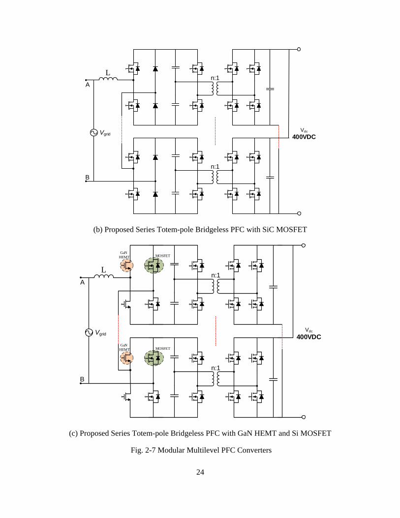
2.1.2.2 Modular multilevel topology
The modular multilevel topology attracts attention due to it being scalable and modular. The
voltage stress is decided by the amplitude of input ac voltage level and the levels of modulation.
Low voltage switches can be utilized in this topology. Three typical topologies are shown in Fig.
2-7. To reduce the number of switches and further improve the efficiency performance, a cascaded
bridgeless totem-pole PFC through a dual-active bridge feeding a common 400-V dc bus is
proposed as shown in Fig. 2-7 (b) and (c). Different from most of the recent literature, which is
focused on the single TPBC or interleaved TPBC [2.13]-[2.15], is that there are several totem-pole
bridgeless PFC converters connected in series. The dc voltage will be divided by the number of
PFC converters. Hence, voltage stresses of the switches can be reduced to a more managable value.

23
For example, if the PFC output voltage is controlled to 400 V, then 650 V rated devices can be
utilized. The output voltage of PFC converters are integrated with dual-active bridges connected
in parallel to increase the current capability. The galvanic isolation is provided by high-frequency
transformer. There are two differences between Fig. 2-7 (b) and (c): (1) Si MOSFET is replaced
by wide bandgap devices such as GaN or SiC, to overcome the reverse recovery problem; (2)
Diodes are replaced by Si MOSFETs for better efficiency performance.
In the dc/dc stage, cascaded totem-pole converters convert grid voltages to primary dc-bus
voltages voi dual-active bridges, whose outputs are connected in parallel to increase the current
capability, produce a secondary dc output voltage. In the dual-active bridge stage, it can be a half-
bridge or a full-bridge on the primary or secondary side. Regarding the kV-level input ac voltage,
the full-bridge of the DAB primary side may be replaced by a half-bridge topology to further
reduce the high-frequency transformer turns ratio.
(a) Series Diode Bridge and Boost PFC
A
N
L
Vgrid
n:1
n:1
Vdc
400VDC
24
(b) Proposed Series Totem-pole Bridgeless PFC with SiC MOSFET
(c) Proposed Series Totem-pole Bridgeless PFC with GaN HEMT and Si MOSFET
Fig. 2-7 Modular Multilevel PFC Converters
A
B
L
Vgrid
n:1
n:1
Vdc
400VDC
A
B
L
Vgrid
n:1
n:1
Vdc
400VDC
GaN
HEMT MOSFET
GaN
HEMT MOSFET

25
2.1.2.3 Hybrid topology
As shown the configuration of Fig. 2-8 [2.11], the input ac of the hybrid topology is rectified
by a diode full bridge, then through a modular isolated dc/dc converter to generate the dc bus to
loads. The diodes, with appropriate voltage ratings, are required in the hybrid topology.
Fig. 2-8 Multi-Cell Boost Topology with Four Input Series Output Parallel Connected Converter
In summary, a modular multilevel H-bridge converter topology and series dual-boost
bridgeless PFC are investigated in this dissertation. Compared with existing topologies in Fig. 2-6,
Fig. 2-7(a) and Fig. 2-8, along with the modularity and scalability, the proposed topology has
additional merits such as:
(a) Better reverse recovery performance of diode by utilizing wide bandgap devices to improve
efficiency performance;
(b) In each cell, two switches are operated at line frequency thereby further reducing power
losses;

26
(c) Fewer active switches. The auxiliary gate driver circuit and power supply are reduced;
(d) Low complexity and low control effort.
2.1.2.4 The proposed topology in low, medium and high power rated data centers
According to [2.16] and [2.17], the sizes of data centers vary widely. Two thirds of data centers
in US are rated at less than 1 MW critical power. To reduce the construction and operation cost of
data centers, multiple companies are sharing one data center, the resulting arrangement is called
co-location data centers. The critical power of co-location data center is usually rated from 10-20
MW. Very few data centers exceed a power rating of 30 MW. At different power ratings, the
prosed topology is modular to achieve high power capability. Three examples are given in the
flowing sections for 1 MW, 10 MW and 30 MW power data centers.
2.1.2.4.1 Low power rating data center (≤ 1 MW)
The proposed topology for a 1 MW data center is shown in Fig. 2-9. If the grid side voltage is
2.4 kV per phase, then the minimum dc bus voltage in the rectifier stage is 3.771 kV. The dc
reference voltage of each totem-pole PFC is set as 800 V, thus at least five cells of totem-pole PFC
converters connected in series to realize 800 V dc output in each PFC stage. To step down 800 V
to 400 V and provide galvanic isolation, a dual-active bridge converter is applied in dc/dc stage.
The 1.2 kV or 1.7 kV SiC MOSFET can be utilized in the proposed topology.

27
Fig. 2-9 Proposed Topology for 1 MW Power Data Center
The rectifier dc bus voltage is calculated below:
The rms voltage of the input ac voltage vac.rms is 2400 V, if the modulation index M is selected
as 0.9, then the minimum voltage of the rectifier dc bus should be:
The reference voltage of each PFC dc bus is selected as 800 V, then the stages of PFC converter
is:
So at least a 5-stage PFC is required. In the three-phase ac grid connected to a 1 MW data
center with a desired efficiency of 99%, the power rating of each stage of the dual-active bridge or
PFC converter is:
A
B
L
Vgrid
2.4 kVAC
1:1
Vdc
400VDC
Vdc1
800 VDC
S1
S2
D1
D2
S3
S4
S5
S6
S7
S8
Cell 1
Cell 2
Cell 3
Cell 4
Cell 5
kVVM
vv rmsac
dcac 771.39.0
240022 .
2
(2-1)
71.4800
771.3,
V
kVn idealPFC
(2-2)
MWMW
p DABPFC 3367.0%993
1,
(2-3)

28
Then the rms current rating for each phase is calculated as shown below:
The peak current is:
If the secondary side dc bus voltage of the dual-active bridge is 400 V, then the current rating
of the switching is:
The voltage/current stress and the available manufacturer of switches are summarized in Table
2.2.
Table 2.2 Switch Specification in 1 MW Data Center
Switch S1-S2, S3-S4 D1~D2 S5-S6, S7-S8
Voltage
stress 800 V 800 V 400V
Current
stress 198.4 A 198.4 A 168.35 A
Manufacturer
CREE, Wolfspeed
Powerex Inc.
CREE, Wolfspeed
Part No. CAS300M17BM2 LS411860 CAS300M17BM2
Voltage
Rating 1.7 kV 1.8 kV 1.7 kV
Current
Rating 225 A(90 ℃), 325 A(25 ℃) 600 A(25 ℃)
225 A(90 ℃), 325
A(25 ℃)
AV
MW
v
pi
rmsac
DABPFC
rmsac 3.1402400
3367.0
.
,
, (2-4)
AAii rmsacpeakac 4.1983.14022 ,, (2-5)
AV
MW
vn
pi
rmsacPFC
DABPFC
outDAB 35.1684005
3367.0
.
,
,
(2-6)

29
Table 2.2 (Cont.) Switch Specification in 1 MW data center
Manufacturer
ROHM
IXYS
ROHM
Part No. BSM300D12P2E001 MDO500-22N1 BSM300D12P2E001
Voltage
Rating 1.2 kV 1.8 kV 1.2 kV
Current
Rating 300 A(60℃) 560 A(25 ℃) 300 A(60 ℃)
Manufacturer
Semikron
Microsemi Power
Products Group
Semikron
Part No. SKM500MB120SC APT30SCD120B SKM500MB120SC
Voltage
Rating 1.2 kV 1.2 kV 1.2 kV
Current
Rating
541 A(25 ℃), 431 A(80
℃)
99 A(25 ℃), parallel
three switches = 297 A
541 A(25 ℃), 431
A(80 ℃)
2.1.2.4.2 Medium and high power rating data center (1~30 MW)
Due to the high power rating, to reduce the current stress of switches, higher ac voltage is
considered. The tradeoff is that the higher the ac voltage, the higher the output dc voltage of the
PFC stage, then more PFC converters and high voltage rating devices are required. This
dissertation evaluates the available 1.2 kV or 1.7 kV SiC MOSFET devices and 4 kV grid side
voltage for a 10 MW data center. The proposed topology is shown in Fig. 2-10. Compared with
the 1 MW data center, to further reduce the current stress of switches, there are four cells of SST
converters, and the number of PFC converters are increased to eight.

30
In the 30 MW data center which is shown in Fig. 2-11, the grid voltage is increased to 6 kV.
There are 12 cells of PFC converters, and 6 cells of SST converters. The equations to calculate the
switch voltages and currents are similar with the previous section. The available switches are
summarized in Table 2.3. With the development of high voltage rating SiC modules, such as the
3.3 kV, 6 kV, 10 kV and 15 kV voltage levels, the number of stages of the proposed topology can
be greatly reduced.
(a) Four cells of SST Converter ac to dc Voltage
kV AC Bus
4 SST Structures
400VDC

31
(b) Each cell has 8 PFC+DAB Converters
Fig. 2-10 Proposed Topology for 10 MW Power Data Center
Table 2.3 Switch Specification in 10 MW Data Center
Switch S1-S2, S3-S4 D1~D2 S5-S6, S7-S8
Voltage rating 800 V 800 V 400V
Current rating 297.7 A 297.7 A 263.1 A
Manufacturer CREE, Wolfspeed Powerex Inc. CREE, Wolfspeed
Part No. CAS300M17BM2 LS411860 CAS300M17BM2
Parallel Device Yes, two switches No Yes, two switches
Manufacturer ROHM IXYS ROHM
Part No. BSM300D12P2E001 MDO500-22N1 BSM300D12P2E00
1
Parallel Device Yes, two switches No Yes, two switches
Manufacturer Semikron Microsemi Power
Products Group Semikron
Part No. SKM500MB120SC APT30SCD120B SKM500MB120SC
Parallel Device Yes, two switches Yes, three switches Yes, two switches
A
B
L
Vgrid
4 kVAC
1:1
Vdc
400VDC
Vdc1
800 VDC
S1
S2
D1
D2
S3
S4
S5
S6
S7
S8
Cell 1
Cell 2
Cell 7
Cell 8

32
(a) 6 cells of SST Converter ac to dc Voltage
(b) Each Cell Has 12 PFC+DAB Converters
Fig. 2-11 Proposed Topology for 30 MW Power Data Center
kV AC Bus
6 SST Structures
400VDC
A
B
L
Vgrid
4 kVAC
1:1
Vdc
400VDC
Vdc1
800 VDC
S1
S2
D1
D2
S3
S4
S5
S6
S7
S8
Cell 1
Cell 2
Cell 11
Cell 12

33
2.1.3 Design of cascaded scaled-down totem-pole multilevel converter
In order to evaluate the proposed topology, a scaled-down prototype was developed and
constructed. Two totem-pole Bridgeless PFC converters are connected in series, shown in Fig.
2-12.
Fig. 2-12 Totem-pole Bridgeless PFC Converter, Two Cells
The circuit design of the proposed topology is introduced in the following section.
2.1.3.1 Switch selection
The switch current is_peak is given by Eq. (2-7).
vdc
N:1
S1
S2
D11
D12
S7
S8
S9
S10
S3
S4
S5
S6
S11
S12
D21
D22
S17
S18
S19
S20
S13
S14
S15
S16
Co1
Co2vo2
vo1
N:1
Cascaded Totem-pole PFC Dual-active Bridge feeding a common 400 V dc bus
idc
Ccbb
A
B
Lg
vgrid
is
vo1
vo2
Co2
Co1
+
-+
-
io1
io2
sgridspeaks vPi 2_ (2-7)

34
where, Ps is the power rating of the proposed topology, vgrid is the rms voltage and frequency of
grid, ηs is the system designed efficiency.
Based on this calculation, the selection of switches are shown in Table 2.4.
Table 2.4 Switch Specification in the Scaled-down ac/dc Converter
Switch MOSFETs in primary
side Diodes in primary side
MOSFETs in
secondary side
Voltage rating 400 V 400 V 400V
Current rating 6 A 6 A 2.53 A
Manufacturer CREE, Wolfspeed Fairchild Semiconductor CREE, Wolfspeed
Part No. C3M0065090D L RHRP15120 C3M0065090D
Voltage
Rating
900 V 1.2 kV 900 V
Current
Rating
36 A(25 ℃), 23 A(100
℃)
15 A(25 ℃) 36 A(25 ℃), 23
A(100 ℃)
2.1.3.2 Grid side inductor design
The grid side inductor is used to reduce the current ripple and reduce the THD of input current.
The inductance is calculated as follows.
The duty cycle for the peak voltage is:
where nPFC is the number of the cascaded bridgeless totem-pole converters and Vo_ref is the desired
dc bus voltage.
The required PFC inductor is analyzed in [2.18]:
where fPFC is the switching frequency of ac/dc stage. is_ripple is the input current ripple requirement.
PFCrefo
gridPFCrefo
PFCnV
vnVD
_
_ 2 (2-8)
PFC
ripples
PFCgrid
g fi
DvL
_
2 (2-9)

35
For 10% ripple:
2.1.3.3 Rectifier dc bus capacitance requirement
There is a double-line frequency ripple voltage in the output dc voltage of the PFC due to the
utilization of single phase rectifier. A capacitor is needed to suppress this voltage ripple. The
following equations are used to calculate the required capacitance. The required dc bus capacitance
is given in the following equation:
where vdc.ripple is the dc voltage ripple requirement. If the acceptable ripple is 5% of dc bus voltage,
then:
2.1.3.4 Input CBB capacitor selection
The input capacitor on the grid side is utilized to reduce the voltage ripple caused by the
switches [2.18]. The equation to calculate the capacitance is shown below:
where krip is the inductor current ripple coefficient and is selected as 20%, r is ac voltage ripple
coefficient and is chose as 5%.
2.2 Control Strategy: PI Control vs Model Predictive Control
2.2.1 Conventional PI control
In many literatures, the conventional PI controllers are investigated for power converters
[2.19][2.20]. A boost converter is used as an example in the following discussion. Usually, there
peaksripples ii __ %10 (2-10)
2,1,2 _.
iVvnf
PC
reforippleDCPFCsgrid
soi
(2-11)
reforippleDC vv _. %5 (2-12)
rmsacSDPFCSD
pkacSDrip
inrvf
ikC
...
..
2 (2-13)

36
are two control loops, which are shown in Fig. 2-13. The inner loop is the current loop, which
regulates the inductor current along its reference and prevents overcurrent conditions. The outer
loop is the voltage loop, which controls the output voltage to an expected value. The inner and
outer PI controllers are designed based on the state-space equations of the power converter. Despite
the reasonable effectiveness, simple scheme and design procedure of the PI control methods, some
issues still need to be addressed, in particular: too many controller parameters need adjustment
during tuning, switching losses and the stability region is usually changed by circuit conditions.
Another disadvantage is that classical PI control is only suitable for single-input, single-output and
linear systems. Significant control design and parameter tuning efforts are needed for the non-
linear and multi-input, multi-output system.
L
S
D
Coutvoutvin
+
-
+
-
RL
iL
R
(a) Boost Converter
(b) Boost Converter with Classical PI Control
Fig. 2-13 Boost Converter Topology as Example

37
2.2.2 Conventional PI controller design steps for a boost converter
L
S
D
Coutvoutvin
+
-
+
-
RL
iL
R
(a) Switch S On
L D
Coutvoutvin
+
-
+
-
RL
iL
RS
(b) Switch S Off
Fig. 2-14 Equivalent Circuits with Switch On and Off
First, the designer needs to develop the mathematical model of the boost converter.
Considering continuous current mode, when the switch is on, the inductor is charged by the dc
source vin. The equivalent circuit is shown in Fig. 2-14(a). The equations of inductor current and
capacitor voltage are given by
where: vin is the input voltage, RL and L are the boost inductor resistance and inductance,
respectively. iL is inductor current, Cout is the output dc capacitor, R is resistive load, vout is the
output dc voltage.
R
tv
dt
tdvC
dt
tdiLtiRtv
outoutout
LLLin
)()(
)()()(
(2-14)

38
When the switch is off, the inductor is connected to the load, which results in the following
equations:
Combination of Eqs. (2-14) and (2-15) lead to the following solution for the state-space
equations in continuous-time domain:
where:
)(
)()(
tv
titx
out
L ,
RCC
LL
R
A
outout
L
11
1
1,
01
10
2
outC
LA ,
onswitch ,1
offswitch ,0u ,
0
1
LB ,
)()( tvtw in ,
)()( tvty out ,
R
tvti
dt
tdvC
tvdt
tdiLtiRtv
outL
outout
outL
LLin
)()(
)(
)()(
)()(
(2-15)
)()(
)()()(
21
tCxty
tBwtxuAAdt
tdx
(2-16)

39
10C .
Use the mathematical model to calculate the required phase and magnitude margin. This step
can be realized in MATLABTM or PLECSTM. The phase and magnitude margin can be easily read
from the simulation results. For example, Fig. 2-15 shows the phase margin of 81.617 degrees,
and a magnitude of 3.14 dB. The last step is tuning PI parameters to meet the phase and magnitude
margin.
Fig. 2-15 Bode-plot of a Boost Converter in PLECS
In summary, both the control scheme and design procedure of PI controller are simple and
reasonably effective. However, the PI controller is only suitable for linear systems and require
significant efforts with regard to controller parameters tuning. For these reasons, a more effective
and straightforward method of model predictive control is introduced and developed in the next
section.
Frequency [Hz]
Ph
ase
[°]
Mag
nit
ude
[dB
]

40
2.2.3 Model predictive control
Model predictive control is a real time control algorithm to overcome the aforementioned
disadvantages. It utilizes the mathematical model of the plant and selects the appropriate device
switching state to achieve the desired control goals. There are four main elements of model
predictive control. First is the mathematical model of the controlled plant. It is a power converter
continuous-time model which specifies the input-output relation of the voltages and currents. Then
the discrete-time model is derived from continuous-time model to predict the system behavior in
the next switching cycle. Second is the design of the control objectives or cost functions. The cost
functions account for the targeted circuit behaviors. For example, the output voltage of power
converter should accurately track the reference, and the input current should be sinusoidal and
achieve unity power factor. The lower the cost value, the better circuit performance is achieved.
Third, it is based on the control goals to sense the feedback signals. The circuit status such as the
voltage of capacitors or current of inductors are feedback signals which are applied in the
mathematical model to predict the future behavior of the controlled variables.
2.2.4 Discretization method: from continuous-time domain to discrete-time domain
The switching period is relatively small when compare with grid frequency and leads to
Then:
where, ‘k’ means the current switching cycle, and ‘k+1’ means the next switching cycle. Ts is one
switching period.
sTdt
kxkxtdx )()1()( (2-17)
sT
kxkx
dt
tdx )()1()( (2-18)

41
The discretization of continuous-time state-space Eq. (2-16) is illustrated by
where:
)1(
)1()1(
kv
kikx
out
L ,
)(
)()(
kv
kikx
out
L ,
)()( kvkw in .
From the discretized Eq. (2-22), the required feedback signals are inductor current iL and the
output voltage vout. The objective of boost converter is to regulate the output dc voltage vout. The
cost function is defined as the absolute voltage error between output voltage and reference voltage.
Thus, the cost function is given by
The expression of vout(k+1) is given by Eq. (2-24) which is rewritten as
)()(
)()()(
21
tCxty
tBwtxuAAdt
tdx
(2-19)
)()(
)()()()1(
21
kCxky
kBwkxuAAT
kxkx
s (2-20)
)()(
)()()()1( 21
kCxky
kxkBwkxuAATkx s (2-21)
)()(
)()()()1( 21
kCxky
kxkBwkxuAATkx s (2-22)
)1( kvVCost outref (2-23)

42
The switching state u has two status 1 and 0. Thus:
where vout(k) is the feedback signal at time k. vout(k+1) is the predicted value at time k+1. S is the
switch state, when S=1, switch is on, otherwise S=0, switch is off.
The corresponding cost functions:
The procedure to choose the proper switching state is shown in Fig. 2-16. vout(k) is the sensed
signal at the beginning of one switching cycle. Assume switch S will be on or off in this switching
cycle, then the predicted output voltage vout(k+1) can be obtained by Eq. (2-25), respectively.
Through comparing Costu=1 and Costu=0, the switching state with the lower cost value is chosen as
the gate single to switch S. In Fig. 2-16, at time of k+1, because Costu=0 is lower than Costu=1, the
‘off’ control signal is selected for switch S. At time of k+2, Costu=1 is lower than Costu=0, the ‘on’
state is the better choice to achieve smaller voltage error. At time of k+3, Costu=0 is higher than
Costu=1, then the switch should be on. However, there is no switching action needed in this
switching period due to the fact that the switch is already on at time k+2. In this case, the switching
speed is reduced.
RC
Tkvki
C
uTkv
out
soutL
out
sout 2)()(
)1()1( (2-24)
off is Sswitch ,2)()()1(
on is Sswitch ,2)()1(
RC
Tkvki
C
Tkv
RC
Tkvkv
out
s
outL
out
s
out
out
s
outout
(2-25)
off is S switch ,2)()(
on is S switch ,2)(
0
1
RC
Tkvki
C
TVCost
RC
TkvVCost
out
soutL
out
srefu
out
soutrefu
(2-26)

43
Fig. 2-16 The Procedure to Choose the Proper Switching State
In summary, the model predictive control is suitable for both linear and non-linear systems. It
also has fewer control parameters. With the design of cost functions, it can easily realize the multi-
objective control. Despite the disadvantages of the model predictive control, such as the
requirement of both high calculation ability of a controller and the accurate modeling of the system,
it provides the significantly better control performance.
Costu@S=0
Costu@S=1
S=0 S=1 S=1k k+1 k+2 k+3
vout(k)Vo_ref
Voltage
Time
Selected
switch stateMeasured
variable
No-selected
switch state
Reference
voltage
Vout_off(k+1)
vout_on(k+1)Switching
period Ts
Switching
period Ts
Switching
period Ts
Vout_on(k+2) Vout_on(k+3)
Costu@S=1
Costu@S=0
Costu@S=0
Costu@S=1
Vout_off(k+2)Vout_off(k+3)

44
2.2.5 Comparison of PI and MPC
Fig. 2-17 Design Flowcharts of PI and MPC Control
The design flowchart is given in Fig. 2-17. All the steps have been discussed in the previous
section. Both control methods require the mathematical model of the system. The MPC needs more
steps to find the best switching state. However, the PI controller parameter is unchanged during
operation, so it is hard to meet all the circuit conditions. The MPC controller is based on the desired
feedback and circuit model, and the gate control signal is optimized during every switching cycle
to realize the expected circuit performance. What’s more, the hardware cost is similar for both PI
and MPC controllers.
In summary, a simple boost converter is used first to help understand the control theory behind
these two controllers. The controller design for the proposed cascaded bridgeless totem-pole

45
multilevel converter, which is more complicated and has more active switches, will be introduced
in the next section.
2.3 MPC design for Cascaded Bridgeless Totem-Pole Multilevel Converter
Fig. 2-18 Scaled-down Prototype: ac/dc Stage, Two Cells
Several control strategies for cascaded converters, such as level-shift pulse-width modulation
(LSPWM), phase-shift PWM, or sliding mode control, have been developed [2.21][2.22]. Despite
the effectiveness of the developed control methods, some issues still need to be addressed, in
particular: voltage balancing, voltage error elimination and switching losses. A model predictive
control through the selection of the appropriate switching state to achieve the control goals has
been applied in motor drives, dc/dc converters and so on [2.23][2.24]. The main characteristic of
the MPC algorithm is predicting the future behavior of the controlled variables whose values will
S1
S2
D11
D12
S11
S12
D21
D22
Co1
Co2vo2
vo1
Cascaded Totem-pole PFC
A
B
Lg
vs
is
io1
io2
RLg

46
be used to calculate the cost function that represents the control objectives of system. The desired
switching states will be obtained by selecting the minimal cost function. In this paper, a real-time
MPC is designed for the proposed cascaded bridgeless totem-pole converter to achieve a better
dynamic performance.
This section is organized as follows: the circuit design of the proposed topology is described
first. Second, the control strategy of the MPC is presented. Third, the simulation and experimental
results of the conventional PI and proposed MPC controller are illustrated. The conclusion and
future work are given in the last part of this section.
2.3.1 Cascaded totem-pole converter modeling
The procedure to design the MPC controller for a two-cell cascaded totem-pole converter will
be discussed in this section. Based on KCL and KVL, in Fig. 2-18, the input-output relationship of
the currents and voltages are given by Eqs. (2-27) (2-28) and (2-29).
where, is is the grid current, Lg is the grid side inductor, RLg is the resistance of inductor, vo1 and vo2
are the 1st cell and 2nd cell output voltages, respectively. Capacitors Co1 and Co2 are the 1st cell and
2nd cell dc-bus capacitor voltages, respectively. u1 and u2 are the switch states of s1 and s2,
respectively. u11 and u12 are the switch states of s11 and s12, respectively.
)()()()()()()(
21211121 tvuutvuutvtiRdt
tdiL oossLg
sg (2-27)
)()()()(
121
1
1 titiuudt
tdvC os
o
o (2-28)
)()()()(
212112
2 titiuudt
tdvC os
oo (2-29)

47
From the time-domain equations, the state-space equations of the cascaded totem-pole
converter are shown in Eq. (2-30).
The expression of x(t), u(t), A1, A2, B, and C are shown below.
1 2
( )( ) ( ) ( )
( ) ( )
dx tA A u t x t Bw t
dt
y t Cx t
(2-30)
)(
)(
)(
)(
2
1
tv
tv
ti
tx
o
o
s
(2-31)
1
0 0
0 0 0
0 0 0
gL gR L
A
(2-32)
21
2
10 0
1 0 0
10 0
g
o
o
L
AC
C
(2-33)
1
2
1 0 0
10 0
10 0
g
o
o
L
BC
C
(2-34)
)(
)(
)(
)(
2
1
ti
ti
tv
tw
o
o
s
(2-35)
)(
)()(
2
1
tv
tvty
o
o (2-36)

48
The discrete-time models from the continuous-time model are given in Eqs. (2-38), (2-39) and
(2-40).
where, ‘k’ means the current switching cycle, and ‘k+1’ means the next switching cycle. Eqs. (2-39)
and (2-40) are to predict the desired control variables vo1(k+1) and vo2(k+1), respectively.
2.3.2 Cost function of totem-pole converter
The control goals of the cascaded totem-pole converter are shown below:
(a) The input current should be sinusoidal and achieve unity power factor.
(b) The output voltage of each totem-pole should accurately track the reference value. The
voltages of the dc buses should be balanced.
(c) Maintain a low switching frequency in order to reduce power losses.
(d) Have a very good dynamic performance against load changes.
0 1 0
0 0 1C
(2-37)
)()(
)()(
)()(
)()1(
212113
1212
1
321
kvuu
kvuu
kiRkv
kiL
Tki
o
o
sLs
s
g
ss
(2-38)
)()()()()1( 1121
1
1 kvkikiuuC
Tkv oos
o
s
o (2-39)
)()()()()1( 221211
2
2 kvkikiuuC
Tkv oos
o
so (2-40)

49
2.3.2.1 Unity power factor control
The goal of power factor correction control is to make the input current waveform sinusoidal
and in phase with the input voltage. The reference current is_ref is controlled by the output of voltage
loop. Then the cost function of PFC control in the proposed topology is given in Eq. (2-41).
2.3.2.2 Voltage balance control
If the PFC rectifier converters are connected in series, the voltage unbalance in the PFC output
side voltage will happen without proper control. The unbalance issue is due to the varied active
power of the DAB and the unequal switching losses in each PFC converter. The difference of these
voltages will lead to the overvoltage of switches and capacitors. There are many papers which
discuss about controlling the voltage unbalance. The existing normal control is utilizing PI or
Proportional-Resonant (PR) control to track dc voltage reference or power reference [2.25]. The
disadvantage of the PI or PR method is that it is not easy to find the proper parameters and the
stability region is usually changed by circuit conditions. What’s more, if the system is nonlinear,
significant parameter design changes are required in PI or PR control. To overcome the
aforementioned disadvantages, the model predictive control is developed in this dissertation.
Without any PI or PR controller, the cost function of the voltage tracking control and voltage
balance are given in Eq. (2-42) and Eq. (2-43), respectively. The simulation results are shown in
Fig. 2-19.
)1(_ kiiCost srefscurrent (2-41)
)1()1( 2_1_ kvVkvVCost orefoorefodc (2-42)
)1()1( 12, kvkvCost oobalancedc (2-43)

50
(a) Without to With Voltage Balance Control
(b) With to Without Voltage Balance Control
Fig. 2-19 Simulation Results of 400 dc Bus Balance Performance
2.3.2.3 Switching sequence
As shown in Table 2.5, there are 16 cases of switching states for switches S1, S2, S11, and S12.
However, S1 and S2 or S11 and S12 should not be ON at the same time to prevent a short circuit, thus
the switching cases 10 to 16 should be avoided. The possible switching states are from cases 1 to
9. The minimum cost function and the related switch positions are applied to the circuit to achieve
the optimized performance of the power converter.
Without proposed balance
control
Without proposed balance
control
DC
bus
volt
age
[V]
DC
bus
volt
age
[V]
Time [ms/div]
Time [ms/div]

51
Table 2.5 Switching Cases of Cascaded Bridgeless Totem-pole PFC
Switching case n
1: switch on
0: switch off
u1 u2 u11 u12
Case 1: 0 0 0 0
Case 2: 0 0 0 1
Case 3: 0 0 1 0
Case 4: 1 0 0 0
Case 5: 1 0 0 1
Case 6: 1 0 1 0
Case 7: 0 1 0 0
Case 8: 0 1 0 1
Case 9: 0 1 1 0
Case 10: 0 0 1 1
Case 11: 1 0 1 1
Case 12: 0 1 1 1
Case 13: 1 1 0 0
Case 14: 1 1 0 1
Case 15: 1 1 1 0
Case 16: 1 1 1 1
2.3.2.4 Overall system cost function
In summary, by combining the aforementioned cost functions, the overall system cost function
is given in Eq. (2-44).

52
The flowchart of the MPC strategy is illustrated in Fig. 2-20. First, the current is(k) of inductor
Lg, and the totem-pole PFC output voltage vo1(k) and vo2(k) are the measured variables at the
beginning of the kth switching cycle. Second, from the discrete-time model in Eqs. (2-38), (2-39)
and (2-40), the variables is(k+1), vo1(k+1) and vo2(k+1) in the (k+1)th switching cycle are predicted.
Third, there are 9 switching cases leading to 9 sets of predictive variables. From each set of
predictive variables, the cost function Costmin is calculated separately. The minimal cost function is
selected and the related switching signals are sent to the gate drive circuit to regulate the expected
dc bus voltage.
balancedcswicthswicthcurrentdc
swicth
swicth
srefscurrent
orefoorefodc
oobalancedc
CostCostCostCostCostCost
kukukukuCost
kukukukuCost
kiiCost
kvVkvVCost
kvkvCost
,12,112,1min
1212111112,11
22112,1
_
2_1_
12,
)1()()1()(
)1()()1()(
)1(
)1()1(
)1()1(
(2-44)

53
Fig. 2-20 The Flowchart of MPC
2.3.3 Block diagram of controllers
The block diagram of the MPC control for the proposed topology is illustrated in Fig. 2-21 (a).
The reference iref in the current-loop is generated by the dc voltage-loop. The voltage-loop aims to
maintain the primary dc bus voi. The controller Gv can be a simple PI or PR control. The
conventional double-loop PI control is also given in Fig. 2-21 (b) for comparison purposes. A more
detailed control loop design given in [2.26]. There are four controllers that need to be designed
which are cumbersome and dependent on each other. The control diagram for the DAB is using
conventional phase-shift control [2.27].

54
(a) MPC Algorithm for the Proposed Topology
(b) Conventional PI Control for the Proposed Topology
Fig. 2-21 The Block Diagram of MPC and Conventional PI for the Proposed Topology
2.3.4 Simulation and experiment verification
In order to verify the effectiveness of the proposed MPC strategy, both simulation and
experimental results are presented. The simulation results are introduced first.
MATLAB/SimulinkTM is used to verify the proposed MPC strategy in the scaled-down 5 kW
prototype. The grid voltage is 480 V and the frequency is 60 Hz. Using Eqs. (2-9) and (2-11), the
boost inductor Lg is 7.2 mH, and the capacitors Co1 and Co2 on the dc side of the totem-pole
converter are 680 μF. Each cell’s dc reference voltage is Vo_ref = 400 Vdc. A resistive load is
connected in the secondary side of the DAB. Conventional PI control and MPC are applied in the
cascaded totem-pole PFC, respectively. The same controller for the DAB is used for both the PI
and MPC controllers.
Gv
iref Eqs.
(6)
(7)
(8)
is, vs
io1, vo1
io2, vo2
Cost
Function
Eq. (9)
Cascaded
Totem-
pole PFC:
S1, 2, 11, 12
u1
u2
MPCVo_ref
vo1+vo2
+-
1/2u11
u12
Vo_ref
vo1
+- +-PI
vo_ref
vo2
+-
+-PI
PI
PI
+-
+-
Cascaded
Totem-
pole PFC:
S1, 2, 11, 12
Double-loop PI
vs/(vs_rms)2
|is| (vo1-|vs|)/vo1

55
2.3.4.1 Simulation: dc bus voltage balance
Before 0.3 s, the converter operates under no-load condition. At 0.3 s, a 5 kW load is connected.
As shown in Fig. 2-22(a), there is a voltage imbalance issue between vo1 and vo2 before 0.3 s when
using the conventional PI control. Auxiliary and complex balance control is needed in the
conventional PI control. Fig. 2-22(b) shows that the voltage is always balanced between the two
totem-pole converters under MPC control. During the step-up load, the conventional PI control
needs at least 0.3 s to stabilize the output voltage of each totem-pole converter, while the MPC
requires less than 0.05 s to stabilize these voltages. The 120 Hz voltage ripple in the dc bus is limited
to 10 V. The simulation results verified that the transient performance of the MPC controller is
much better than that of the PI controller.
(a) Conventional PI Control
(b) Model Predictive Control
Fig. 2-22 Normal Operation to Step-up Load of the Two Controllers

56
2.3.4.2 Simulation results of switching frequency
The switching frequency of the conventional PI control is set at 20 kHz. The switching
frequency of the MPC is variable and depends on the system feedback. The simulation results of
the gate signal from each controller are shown in Fig. 2-23 and Fig. 2-24. The maximum switching
frequency of the MPC is about 8 kHz. This is less than half of the switching frequency in the
conventional PI control, so the switching loss can be greatly reduced. The current THD of both
controllers are all within the IEEE 519-2014 standard. It is worth mentioning that the minimum
switching frequency of MPC algorithm should be set to meet the THD requirements.
Fig. 2-23 Gate Signals For a Selected Switch Position For Conventional PI Control
Fig. 2-24 Gate Signals for a Selected Switch Position for Model Predictive Control

57
2.3.4.3 Experiment: dc bus voltage balance
The experimental setup is shown in Fig. 2-25 which includes the hardware-in-loop (HIL)
simulator Typhoon HIL402, a TI DSP TMS320F28335 control card, and oscilloscope. The MPC
algorithm is programmed in the DSP. The proposed cascaded bridgeless totem-pole PFC and dual-
active bridge converter are modeled in Typhoon HIL 402. The circuit parameters are the same as
those in the simulation setup. The test results of vo1 and vo2 are shown in Fig. 2-26 and Fig. 2-27,
respectively. Similarly to the simulation results, the experimental results exhibit that the proposed
MPC strategy has smaller overshoot and much faster response when the load power changes from
0 to 5 kW.
Fig. 2-25 Experimental Setup: Typhoon Simulator and DSP Control Card

58
Fig. 2-26 Hardware-In-Loop Testing Results of Conventional PI Control (Time: 25 ms/div,
vo1=vo2=400 V, iload: 0 to 12.5 A)
Fig. 2-27 Hardware-In-Loop Testing Results of The Proposed Model Predictive Control (Time:
25 ms/div, vo1=vo2=400 V, iload: 0 to 12.5 A)
2.4 Conclusion
A model predictive control for a novel cascaded bridgeless totem-pole multilevel converter for
400 V DC-powered data centers was presented. The procedures to design MPC control in power
converter application are:
(a) Determination of power converter model to specify the input-output relation of the voltages
and currents.

59
(b) Determination of discrete-time model from continuous-time model to predict the system
future behavior.
(c) Designing the cost functions. In the proposed topology, the first cost function can be that
the sinusoidal input current to meet a unity power factor requirement. Second, the output voltage
of each totem-pole should accurately track the reference value. The third cost function is to limit
the switching frequency to a set range to minimize loss while optimizing filter performance. Fourth,
is to ensure good dynamic response during load changes.
(d) Select the switch position to have the minimum cost function and apply it to circuit to
achieve the preferred performance of power converter.
Compared with existing multilevel converters, totem-pole converters, by utilizing the
advantages of wide bandgap devices, were cascaded to achieve high efficiency and reduce the
number of active switches. Compared to the conventional PI control, the proposed MPC strategy
had better transient and voltage balance performance and required lower switching frequencies
which translates to lower switching losses. Both simulation and experimental results were been
presented to validate the effectiveness of the proposed topology and its optimized MPC strategy.
The disadvantage of MPC is that it requires high calculation ability of a controller and accurate
modeling of the system. Thanks to the rapid development of the micro-processor, the
computational ability of state-of-the-art DSPs have been greatly improved. For example, the clock
frequency of TMS320F28377D DSP is 200 MHz, the MPC algorithm can be easily implemented
in such a DSP.

60
2.5 Reference
[2.1] K. S. B. Muhammad and D. D. C. Lu, "ZCS Bridgeless Boost PFC Rectifier Using Only
Two Active Switches," in IEEE Transactions on Industrial Electronics, vol. 62, no. 5, pp.
2795-2806, May 2015.
[2.2] L. Huber, Y. Jang and M. M. Jovanovic, "Performance Evaluation of Bridgeless PFC Boost
Rectifiers," in IEEE Transactions on Power Electronics, vol. 23, no. 3, pp. 1381-1390,
May 2008.
[2.3] B. Su, J. Zhang and Z. Lu, "Totem-Pole Boost Bridgeless PFC Rectifier With Simple Zero-
Current Detection and Full-Range ZVS Operating at the Boundary of DCM/CCM," in
IEEE Transactions on Power Electronics, vol. 26, no. 2, pp. 427-435, Feb. 2011.
[2.4] “eGaN® FET Characteristics.” [Online]. Available: http://epc-
co.com/epc/FAQ/eGaNFETCharacteristics.aspx.
[2.5] J. Millán, "A review of WBG power semiconductor devices," CAS 2012 (International
Semiconductor Conference), Sinaia, 2012, pp. 57-66.
[2.6] “SiC Power Devices and Modules.” [Online]. Available:
http://rohmfs.rohm.com/en/products/databook/applinote/discrete/sic/common/sic_appli-
e.pdf.
[2.7] Y. Yang, M. Mu, Z. Liu, F. C. Lee and Q. Li, "Common mode EMI reduction technique
for interleaved MHz critical mode PFC converter with coupled inductor," 2015 IEEE
Energy Conversion Congress and Exposition (ECCE), Montreal, QC, 2015, pp. 233-239.
[2.8] Z. Liu, Z. Huang, F. C. Lee, Q. Li and Y. Yang, "Operation analysis of digital control based
MHz totem-pole PFC with GaN device," Wide Bandgap Power Devices and Applications
(WiPDA), 2015 IEEE 3rd Workshop on, Blacksburg, VA, 2015, pp. 281-286.
[2.9] C. Marxgut, F. Krismer, D. Bortis and J. W. Kolar, "Ultraflat Interleaved Triangular
Current Mode (TCM) Single-Phase PFC Rectifier," in IEEE Transactions on Power
Electronics, vol. 29, no. 2, pp. 873-882, Feb. 2014.
[2.10] J. W. Kolar, G. Ortiz, “Solid-state-transformers: Key components of future traction and
smart grid systems,” in Proceedings of the International Power Electronics Conference,
IPEC 2014, Japan, May 18-24, 2014.
[2.11] D. Rothmund, G. Ortiz and J. W. Kolar, "SiC-based unidirectional solid-state transformer
concepts for directly interfacing 400V DC to Medium-Voltage AC distribution
systems," 2014 IEEE 36th International Telecommunications Energy Conference
(INTELEC), Vancouver, BC, 2014, pp. 1-9.
[2.12] D. Rothmund, G. Ortiz, T. Guillod and J. W. Kolar, "10kV SiC-based isolated DC-DC
converter for medium voltage-connected Solid-State Transformers," 2015 IEEE Applied

61
Power Electronics Conference and Exposition (APEC), Charlotte, NC, 2015, pp. 1096-
1103.
[2.13] Z. Huang, Z. Liu, Q. Li and F. C. Lee, "Microcontroller-based MHz totem-pole PFC with
critical mode control," 2016 IEEE Energy Conversion Congress and Exposition (ECCE),
Milwaukee, WI, 2016, pp. 1-8.
[2.14] Z. Liu, Z. Huang, F. C. Lee and Q. Li, "Digital-Based Interleaving Control for GaN-Based
MHz CRM Totem-Pole PFC," in IEEE Journal of Emerging and Selected Topics in Power
Electronics, vol. 4, no. 3, pp. 808-814, Sept. 2016.
[2.15] R. S. c. Yeung, J. W. t. Fan and H. S. h. Chung, "A totem-pole PFC using hybrid pulse-
width-modulation scheme," 2017 IEEE 3rd International Future Energy Electronics
Conference and ECCE Asia (IFEEC 2017 - ECCE Asia), Kaohsiung, 2017, pp. 1286-1290.
[2.16] J. G. Koomey. Growth in Data Center Electricity Use 2005 to 2010. Analytics Press, 2011.
[2.17] U.S. Environmental Protection Agency. Report to Congress on server and datacenter
energy effiency. Public Law 109-431, August 2, 2007.
[2.18] X. She, A. Q. Huang and G. Wang, "3-D Space Modulation With Voltage Balancing
Capability for a Cascaded Seven-Level Converter in a Solid-State Transformer," in IEEE
Transactions on Power Electronics, vol. 26, no. 12, pp. 3778-3789, Dec. 2011.
[2.19] L. Huber, M. Kumar and M. M. Jovanović, "Performance Comparison of PI and P
Compensation in DSP-Based Average-Current-Controlled Three-Phase Six-Switch Boost
PFC Rectifier," in IEEE Transactions on Power Electronics, vol. 30, no. 12, pp. 7123-
7137, Dec. 2015.
[2.20] Z. Chen, "PI and Sliding Mode Control of a Cuk Converter," in IEEE Transactions on
Power Electronics, vol. 27, no. 8, pp. 3695-3703, Aug. 2012.
[2.21] A. Nami, J. Liang, F. Dijkhuizen and G. D. Demetriades, “Modular Multilevel Converters
for HVDC Applications: Review on Converter Cells and Functionalities,” in IEEE
Transactions on Power Electronics, vol. 30, no. 1, pp. 18-36, Jan. 2015.
[2.22] S. Debnath, J. Qin, B. Bahrani, M. Saeedifard and P. Barbosa, “Operation, Control, and
Applications of the Modular Multilevel Converter: A Review,” in IEEE Transactions on
Power Electronics, vol. 30, no. 1, pp. 37-53, Jan. 2015.
[2.23] M. Cheng, F. Yu, K. T. Chau and W. Hua, “Dynamic Performance Evaluation of a Nine-
Phase Flux-Switching Permanent-Magnet Motor Drive With Model Predictive Control,”
in IEEE Transactions on Industrial Electronics, vol. 63, no. 7, pp. 4539-4549, July 2016.
[2.24] M. Mosa; R. Balog; H. Abu-Rub, "High Performance Predictive Control of Quasi
Impedance Source Inverter," in IEEE Transactions on Power Electronics , vol.PP, no.99,
pp.1-1, 2016.

62
[2.25] X. She, “Control and Design of a High Voltage Solid State Transformer and its Integration
with Renewable Energy Resources and Microgrid System”, Ph.D thesis, NCSU, 2013.
[2.26] L. Zhou, Y. Wu, J. Honea and Z. Wang, “High-efficiency True Bridgeless Totem Pole PFC
based on GaN HEMT: Design Challenges and Cost-effective Solution,” PCIM Europe
2015; International Exhibition and Conference for Power Electronics, Intelligent Motion,
Renewable Energy and Energy Management, Nuremberg, Germany, pp. 1-8, 2015.
[2.27] Y. Zhang, J. Umuhoza, H. Liu, C. Farrell and H. A. Mantooth, “Optimizing efficiency and
performance for single-phase photovoltaic inverter with dual-half bridge converter,” 2015
IEEE Applied Power Electronics Conference and Exposition (APEC), Charlotte, NC, pp.
1507-1511, 2015.

63
CHAPTER 3
MODELING AND CONTROL OF SOLID STATE TRANSFORMER DC/DC STAGE:
EFFICIENCY IMPROVEMENT
3.1 Introduction and Motivation
In the dc/dc stage, the dual-active bridge converter is well adapted for this application due to
its excellent performance in voltage conversion, flexibility, high power density, galvanic isolation,
modularity and high efficiency [3.1]-[3.4].
The conventional single phase-shift (SPS) modulation control is simple and easy to implement
in many applications [3.5]-[3.7]. In order to improve the efficiency performance of the DAB, the
SPS has been improved by using the multi-phase-shift control, such as extended phase-shift (EPS),
dual phase-shift (DPS) and triple phase-shift (TPS) controls [3.8]-[3.10]. These three phase-shift
control methods are classified by the different phase-shift angles, reducing the current stress and
circulating energy in the circuits, thus the efficiency performance is improved. The TPS control is
recognized as a unified phase-shift control, but the penalty of this control method is much
complexity and increased design efforts. Compare with other phase-shift strategies, the DPS
control has been popular due to its efficiency performance and its acceptable level of complexity.
To further increase the power efficiency of the DAB, the multi-phase-shift controls are designed
with the goal of minimum current stress [3.11] or minimum reactive power flow [3.12]. These two
efficiency optimization methods can reduce the power loss in the DAB, but neither is a
straightforward method. A more optimal strategy which can find the desired phase-shift angles

64
directly from the power loss model of the DAB. In the paper [3.13], a conventional loss model is
utilized in an IGBT-based DAB. The saturation voltage of the IGBT along with the voltage drop
of the diode are assumed as constant values. These assumptions may prevent the algorithm from
calculating the expected phase-shift angle and couldn’t guarantee the high efficiency performance.
To increase the power density of the DAB wide bandgap devices, such as SiC MOSFETs or GaN
FETs, are usually utilized today. Different from the IGBT, the MOSFET can have bidirectional
current flow when its gate voltage is high enough, thus the operation of the MOSFET version of
the DAB also differs from the DAB which utilizes IGBTs.
Compared with the aforementioned studies, a more accurate loss model is developed in this
work to further improve the efficiency performance of the SiC-based dual-active bridge. A
comprehensive operational analysis of the SiC-based DAB is also presented in this work. A
detailed improved conduction loss model and switching loss model are given to construct a more
accurate loss model of the DAB. For example, the loss model of a DAB will consider the effect of
junction temperature, gate resistance, and gate voltage to the power loss. Furthermore, the impact
of harmonic currents, as they relate to the losses, on auxiliary circuits and transformers is illustrated.
According to the comparison of the proposed loss model with the aforementioned control of a SiC-
based DAB from the experimental prototype testing results, the efficiency of the DAB is improved
with varying input voltages and/or load power.
This chapter is organized as follows: Section II introduces the SiC MOSFET-based DAB
operation principle. A simplified power loss model and an improved power loss model are
presented in Section III, and finally, the simulation and experimental results are included in Section
IV.

65
3.2 Dual Active Bridge Operation
3.2.1 Single phase-shift control
The single phase-shift control is widely used in the dual-active bridge converter due to its
simplicity. The switches S1-S8 are controlled with a 50% duty cycle. Leg 1 and Leg 3 have the
phase-shift, and leg 2 and leg 4 have the same phase-shifts which are shown in Fig. 3-1. vpri is the
voltage output from the primary side full bridge, and vsec is the voltage input to the secondary side
full bridge. As shown in Fig. 3-2, with changing the phase-shift angle, the voltage across the
inductor Lk will change and then the power flows between the primary and secondary sides. The
disadvantage of single phase-shift control is that the RMS and peak current of the switches are
high due to the circulating power flow in the circuit [3.13], thus the efficiency of DAB with single
phase-shift control is relatedly low.
Fig. 3-1 Dual-Active Bridge with Single Phase-Shift Control
vout
N1:N2
Cin Cout
Lk
S1 S3
S2 S4
S5 S7
S6 S8
vprivseciLk
iC
iDC
Leg 1 Leg 2 Leg 3 Leg 4

66
Fig. 3-2 Single Phase-Shift Control: The Transformer Input/Output Voltage and Inductor Lk
Current
3.2.2 Extended phase-shift control
To reduce the RMS and peak current stress of the switches, while also improving the efficiency,
the EPS control has been investigated in [3.8][3.14]. Comparing with SPS, EPS has the phase-shift
between leg1 and leg2 which is shown in Fig. 3-3. There are two degrees of freedom to change the
voltage difference, thus controlling the power flow. The first degree Do is used to control the
magnitude and direction of power flow. The second degree Di is applied to reduce the circulating
power and current stress of the converter. The detailed inductor voltage and current waveforms are
given in Fig. 3-4.
Dvpri
vsec
v
iL
t
t
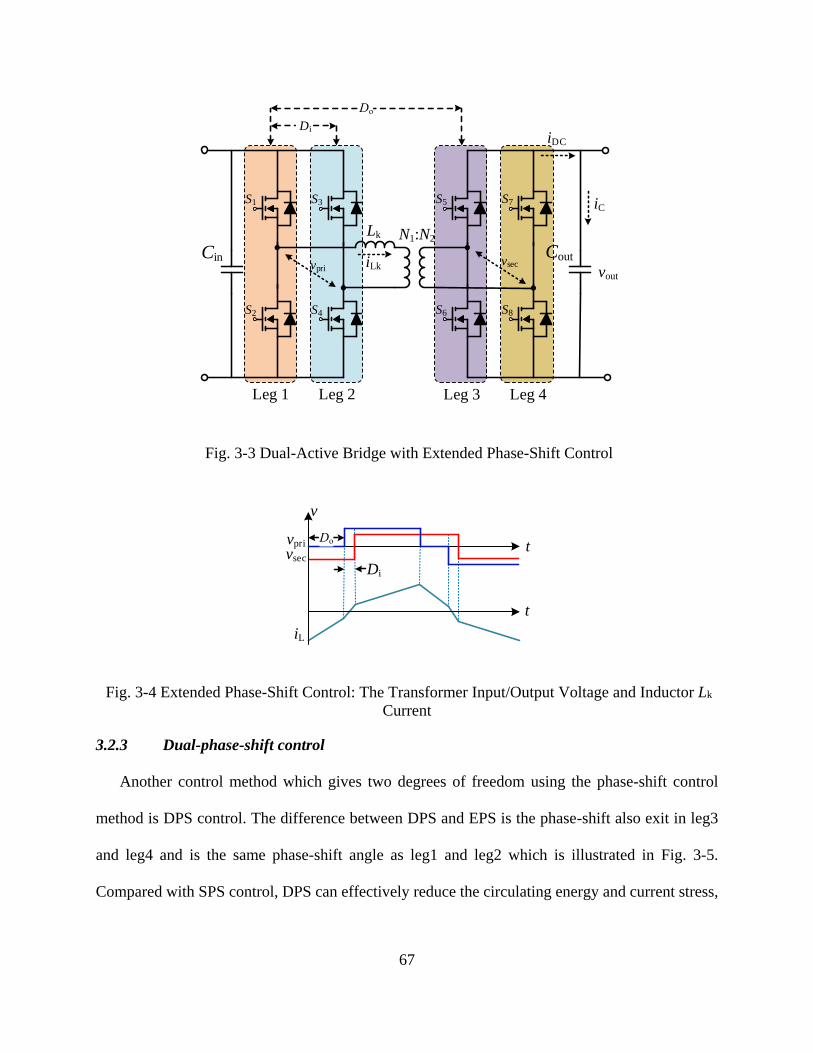
67
Fig. 3-3 Dual-Active Bridge with Extended Phase-Shift Control
Fig. 3-4 Extended Phase-Shift Control: The Transformer Input/Output Voltage and Inductor Lk
Current
3.2.3 Dual-phase-shift control
Another control method which gives two degrees of freedom using the phase-shift control
method is DPS control. The difference between DPS and EPS is the phase-shift also exit in leg3
and leg4 and is the same phase-shift angle as leg1 and leg2 which is illustrated in Fig. 3-5.
Compared with SPS control, DPS can effectively reduce the circulating energy and current stress,
vout
N1:N2
Cin Cout
Lk
S1 S3
S2 S4
S5 S7
S6 S8
vprivseciLk
iC
iDC
Di
Leg 1 Leg 2 Leg 3 Leg 4
vpri
vsec
v
iL
t
t
Di

68
however it also expands the soft-switching range [3.9][3.15]. The inductor voltage and current
waveforms with DPS control is given in Fig. 3-6.
Fig. 3-5 Dual-Active Bridge with Dual Phase-Shift Control
Fig. 3-6 Dual Phase-Shift Control: The Transformer Input/Output Voltage and Inductor Lk
Current
3.2.4 Triple phase-shift control
As shown in Fig. 3-7, the TPS control method has three degrees of freedom [3.16]-[3.18]. The
phase-shift Di1 between leg1 and leg 2 is different with the phase-shift Di2 between leg3 and leg4.
In TPS control, the current stress is reduced and the soft-switching range is wider. The tradeoff is
vout
N1:N2
Cin Cout
Lk
S1 S3
S2 S4
S5 S7
S6 S8
vprivseciLk
iC
iDC
Di1=Di Di2=Di
Leg 1 Leg 2 Leg 3 Leg 4
vpri
vsec
v
iL
t
t
Do
Di
Di

69
that the design of TPS control is much more complicated than that of the SPS, EPS and DPS
control methods. The input and output voltages of the transformer and inductor Lk current are given
in Fig. 3-8.
Fig. 3-7 Dual-Active Bridge with Triple Phase-Shift Control
Fig. 3-8 Triple Phase-Shift Control: The Transformer Input/Output Voltage and Inductor Lk
Current
vout
N1:N2
Cin Cout
Lk
S1 S3
S2 S4
S5 S7
S6 S8
vprivseciLk
iC
iDC
Di1 Di2
Leg 1 Leg 2 Leg 3 Leg 4
vpri
vsec
v
iL
t
t
Do
Di1Di2

70
3.2.5 Conclusion
Comparing these four phase-shift control strategies, the performance of TPS is the best but
also the most complicate. The SPS control is the simplest but the high circulating currents and
RMS or peak current stress. Compare EPS with DPS, the control state of the two full bridges are
changed when the required power or voltage is changed, but DSP control doesn’t, with this reason,
the DPS control is adopted in the following section to achieve a relatively simple, effective and
high efficiency control strategy.
3.3 Efficiency Optimization Methods
To improve the efficiency performance of the dual-active bridge converter, two popular
methods are reported in [3.11][3.19][3.20]: (1) Peak current minimization method and (2)
circulation power reduction method. The drawback of these two methods are the efficiency is not
optimal in the wide range of the load power. A loss model based method is reported in [3.20][3.21].
In the paper [3.20], it is applied with an IGBT based-circuit and simple loss model. It assumed that
the saturation voltage of IGBT and voltage drop of the diode are constant values, thus it may not
realize the optimized efficiency performance. In the last few years, the wide bang-gap device has
been widely used due to its fast switching capability and low on-state resistance, thus it is very
suitable for the dual-active bridge converter application. In this section, a SiC MOSFET based
dual-active bridge is analyzed and a more accurate loss model is developed to achieve better
efficiency performance.
3.3.1 Current stress minimization method
The control diagram of current stress minimization control is given in Fig. 3-9. The PI control
is adopted in the voltage loop to regulate the dc bus voltage at the secondary side. The solved Di

71
is fed as the forward signal added plus with the output of PI controller. The final stage of this
control strategy is the phase-shift generator which can be realized by the controller.
Fig. 3-9 Control Diagram of Current Stress Minimization
The phase-shift Di and Do are calculated by the Lagrangian expression. Lagrangian function is
a strategy to find the minimum or maximum value of an object with some constraints. The normal
Lagrangian expression is shown in Eq. (3-1).
where the function L is called the "Lagrangian", f(x1, x2, …, xn) is the objective function, g(x1,
x2, …, xn) is the constraint function, λ is defined as Lagrange multiplier, c is the desired constant
value of constraint function g(x1, x2, …, xn).
In order to realize the control goal, set the gradient of Lagrangian expression equal to zero:
Ubus_ref
Do,dc
-+ PI
vo
current stress
minimization
vo
io
-+Do
Di
Phase
Shift
PWM
DAB
m
k
nkknmn cxxxgxxxfxxxL1
21212121 )),...,,((),...,,(),...,,,,...,,( (3-1)

72
By solving Eq. (3-2), the desired x1, x2, …, xn can be found to achieve the minimum or
maximum value of control objective.
In the DPS control, the two degrees of control variables are Di and Do, and the Lagrangian
expression is shown in Eq. (3-3).
where ipeak(Di, Do) is the peak current in the DPS control, Pout is the power output of the DPS
control, Pref is the reference power of the dual-active bridge.
The expression of ipeak and Pout can be derived from the current and voltage waveform of the
leakage inductor. By solving Eq. (3-4), the calculated values Di and Do are the desired phase-shifts
which can be realized with the minimum peak current stress.
m
mn
mn
mn
n
mn
mn
mn
xxxL
xxxL
xxxL
x
xxxL
x
xxxL
x
xxxL
),...,,,,...,,(
0),...,,,,...,,(
0),...,,,,...,,(
0),...,,,,...,,(
0),...,,,,...,,(
0),...,,,,...,,(
2121
2
2121
1
2121
2121
2
2121
1
2121
(3-2)
)(),(),,( refoutoipeakoi PPDDiDDL (3-3)

73
3.3.2 Circulating power reduction method
Similar to the current stress minimization control, the Lagrangian expression of the circulating
power reduction method is shown in Eq. (3-5). The circulating power Pcircutlation and output power
of DAB Pout can be derived from the current and voltage waveform of the leakage inductor.
Similar with the current stress optimization control, the desired phase-shift of Di and Do are
solved by Eq. (3-6).
The control diagram of circulating power reduction method is given in Fig. 3-10. The
difference with the current stress minimization control is that the desired phase-shift is based on
the control of minimization of the circulating power.
0
0
0
refout
o
out
o
peak
o
i
out
i
peak
i
PPL
D
P
D
i
D
L
D
P
D
i
D
L
(3-4)
)(),(),,( refoutoincirculatiooi PPDDPDDL (3-5)
0
0
0
refout
o
out
o
ncirculatio
o
i
out
i
ncirculatio
i
PPL
D
P
D
P
D
L
D
P
D
P
D
L
(3-6)

74
Fig. 3-10 Control Diagram of Circulating Power Reduction
In the next section, a loss model based on the efficiency optimization method is proposed. In
order to build the loss model, the operation principle of the dual-active bridge is introduced first,
then the simple and more accurate loss model are developed and compared.
3.4 SiC MOSFET-based DAB Operation Principle
There are two operational conditions of the dual-phase-shift control method, which are Do<Di
and Di<Do, where Di is the inner phase-shift and Do is the outer phase-shift. This dissertation
mainly discusses the case of Di<Do. The analysis steps of Do<Di are the same. The operation
principle of dual-active bridges in the dual-phase-shift model is given in Fig. 3-12. From t0 to t10,
there are 10 stages.
Ubus_ref
Do,dc
-+ PI
vo
circulating
power
reduction
vo
io
-+Do
Di
Phase
Shift
PWM
DAB

75
Fig. 3-11 Control Signal and Circuits Waveform when Di<Do
(a) Stage 10: t9<t10 (b) Stage 1: t0<t1
(c) Stage 2: t1<t2 (d) Stage 3: t2<t3
vgs2 vgs1 vgs2
vgs3 vgs4 vgs3
vgs6 vgs5 vgs6
vgs7 vgs8 vgs7
vpri
vsec
iLkt
t
t
t
t
t
t
v
t0 t1 t2 t4 t5 t6 t8t3 t7 t9 t10
Di*Ths
Di*Ths
Do*Ths
vout
Coutvpri
vsec
S1 S3
S2 S4
S5
S6 S8
S7
Lk
vin
Cin vout
Coutvpri
vsec
S1 S3
S2 S4
S5
S6 S8
S7
Lk
vin
Cin
D1 D3
D2 D4
D5
D6 D8
D7 D1 D3
D2 D4
D5
D6 D8
D7
vout
Coutvpri
vsec
S1 S3
S2 S4
S5
S6 S8
S7
Lk
vin
Cinvout
Coutvpri
vsec
S1 S3
S2 S4
S5
S6 S8
S7
Lk
vin
Cin
D1 D3
D2 D4
D5
D6 D8
D7D1 D3
D2 D4
D5
D6 D8
D7

76
(e) Stage 4: t3<t4 (f) Stage 5: t4<t5
(g) Stage 6: t5<t6 (h) Stage 7: t6<t7
(i) Stage 8: t7<t8 (j) Stage 9: t8<t9
Fig. 3-12 10 Operational Stages when Di<Do
The current equations for 10 stages are given in Table 3.1.
.
Coutvpri
vsec
S1 S3
S2 S4
S5
S6 S8
S7
Lk
vin
Cinvout
Coutvpri
vsec
S1 S3
S2 S4
S5
S6 S8
S7
Lk
vin
Cinvout
D1 D3
D2 D4
D5
D6 D8
D7D1 D3
D2 D4
D5
D6 D8
D7
vout
Coutvpri
vsec
S1 S3
S2 S4
S5
S6 S8
S7
Lk
vin
Cinvout
Coutvpri
vsec
S1 S3
S2 S4
S5
S6 S8
S7
Lk
vin
Cin
D1 D3
D2 D4
D5
D6 D8
D7D1 D3
D2 D4
D5
D6 D8
D7
vout
Coutvpri
vsec
S1 S3
S2 S4
S5
S6 S8
S7
Lk
vin
Cinvout
Coutvpri
vsec
S1 S3
S2 S4
S5
S6 S8
S7
Lk
vin
Cin
D1 D3
D2 D4
D5
D6 D8
D7D1 D3
D2 D4
D5
D6 D8
D7

77
Table 3.1 The Inductor Lk Current Equations, Di<Do
Time
Primary side
ac voltage,
vpri
Secondary
side ac
voltage, vsec
Current equation
t9 ~ t10 -vin -N*vout 9
9LkLksec
)()()(
tt
titiLvv
dt
diLv kprikL
)()()( 9
outin
9LkLk ttL
Nvvtiti
k
t0 ~ t1 0 -N*vout )()()( 0
out
0LkLk ttL
Nvtiti
k
t1 ~ t2 0 -N*vout )()()( 1
out
1LkLk ttL
Nvtiti
k
t2 ~ t3 vin -N*vout )()()( 2
outin
2LkLk ttL
Nvvtiti
k
t3 ~ t4 vin 0 )()()( 3in
3LkLk ttL
vtiti
k
t4 ~ t5 vin N*vout )(-
)()( 4
outin
4LkLk ttL
Nvvtiti
k
t5 ~ t6 0 N*vout )(-
)()( 5
out
5LkLk ttL
Nvtiti
k
t6 ~ t7 0 N*vout )(-
)()( 6
out
6LkLk ttL
Nvtiti
k
t7 ~ t8 -vin N*vout )(--
)()( 7
outin
7LkLk ttL
Nvvtiti
k
t8 ~ t9 -vin 0 )(-
)()( 8in
8LkLk ttL
vtiti
k
Stage 1, t0<t<t1: At time t<t0, S2, S3, S6, and S7 are on. At t0, S3 turns off first. To prevent the dc
bus voltage short through, a short dead time td is set between S3 and S4. The diode D4 is conducting
in freewheeling mode during the dead time. At time t0+td, the gate signal of S4 is high level, then

78
S4 is turned on at zero-voltage switching (ZVS). Due to the fact that MOSFETs allow bidirectional
current flow, a large proportion of current will flow from source to the drain when the gate voltage
is much higher than the threshold voltage. Then diode D4 turns off and leads to reverse-recovery
loss.
Stage 2: The MOSFETs in the primary and secondary sides are still conducting, but the current
direction at both sides are changed at time t1.
Stage 3: At time t<t2, S2, S4, S6 and S7 are on, S2 turns off at time t1, then D2 is conducting as
freewheeling diode. After time t1+td, S1 is turned on at hard switching mode and D2 turns off.
Stage 4: The primary side switches keep the same status as the previous stage, the secondary
side switch S7 is turned off at time t2, D7 conducts during the dead time. At time t2+td, S8 turns on
and D7 is off.
Stage 5: During this stage, S1 and S4 only have conducting loss. S6 turns off at time t4, D5 is on
immediately. At time t4+td, S5 turns on at ZVS.
Stage 6: The secondary side switches S5 and S8 are always on during this stage. S4 turns off and
D3 is on at time t5. S3 turns on at ZVS.
Stage 7: In this stage, the current direction changed in the primary and secondary sides. Only
conduction loss is happened in this stage.
Stage 8. The MOSFET S1 turns off at time t6, then the diode D1 is conducting during dead time.
S2 turns on with hard switching at time t6+td. The status of secondary side switches are the same
as stage 7.

79
Stage 9: The switches of primary side stay the same status as in stage 7. The secondary side
switch S8 turns off at time t7, the diode D8 conducts the current until S7 soft switching turns on.
Stage 10: This stage is the last stage in one switching period. The status of primary side’s
switches are same as in stage 9. S5 is turned off at t9 then D6 is conducting the current. S5 is turned
at ZVS.
From the operational principle of the dual-phase-shift control in the dual-active bridge, the
switching actions are summarized in Table 3.2. The conduction actions are shown in Table 3.3.
Table 3.2 The Switching Actions in One Switching Period
Hard turn-off Soft turn-off Hard turn-on Soft turn-on Diode reverse recovery
S3 at t0,
S7 at t3,
S6 at t4,
S4 at t5,
S8 at t8,
S5 at t9
S2 at t2,
S1 at t7
S1 at t2,
S2 at t7
S4 at t0,
S8 at t3,
S5 at t4,
S3 at t5,
S7 at t8,
S6 at t9
D4 at t0,
D2 at t2,
D8 at t3,
D5 at t4,
D3 at t5,
D1 at t7,
D7 at t8,
D6 at t9
Table 3.3 The Conduction Actions in One Switching Period
Time t0-t1,
t1-t2 t2-t3 t3-t4 t4-t5
t5-t6,
t6-t7 t7-t8 t8-t9 t9-t10
MOSFET S2, S4,
S6, S7
S1, S4,
S6, S7
S1, S4,
S6, S8
S1, S4,
S5, S8
S1, S3,
S5, S8
S2, S3,
S5, S8
S2, S3,
S5, S7
S2, S3,
S6, S7

80
3.5 Simplified Power Loss Model and Improved Power Loss Model
3.5.1 Switching loss analysis and modeling
3.5.1.1 Turn-on loss model
The main turn-on or turn-off power loss happens when the gate voltage is between the thresh
hold voltage Vth and plateau voltage Vplateau. During the turn-on process, when Vgs reaches Vth, the
current path is changed from the body diode to MOSFET. During this period, the power loss can
be calculated as turn-on loss of the MOSFET and reverse-recovery loss of free-wheeling diode.
From the simple turn-on loss calculation method, the current rise time and voltage fall time is
assuming constant values. Thus, from switching scenarios in Fig. 3-11 and Fig. 3-12, the Eq. (3-7)
is presented as the turn-on loss.
where, td,on is turn-on delay time, tr is rise time of switch.
In this work, the more accurate turn-on loss model is considered with the contribution of the
gate voltage, gate resistance and dc bus voltage to the switching loss. The gate resistance should
be adjusted to realize fast turn-on and turn-off but acceptable Vds overshoot. The gate current
during turn-on is shown in Eq. (3-8). The voltage fall time can be calculated in Eq. (3-9). Then,
the turn-on energy loss and the power loss in a switching period are given in Eq. (3-10).
s
rondin
simpleMOSon ftttitiv
P2
)()( ,72
__
, when Di<Do (3-7)
gatedriver
plateaudriver
ongRR
VVi
,
(3-8)

81
where Vdrive is the supplied gate voltage, Rgate is the internal gate resistance, and Rdriver is the
external gate resistance. Cgd1 and Cgd2 are the associated gate capacitance which can be read from
the datasheet. tri is the current rise time which is given in the device datasheet.
3.5.1.2 Turn-off loss model
Same as the turn-on loss model, as given in the Table 3.2, the turn-off loss simple and more
accurate model of SiC MOSFET are given in Eqs. (3-11)(3-12) and Eqs. (3-13)(3-14), respectively.
In the Eq. (3-11), the switch turn-off time parameters are red from the datasheet directly. In the
accurate model as shown in Eq. (3-14), the junction temperature is considered as variable in the
accurate loss model. The gate resistance and voltage are used in the turn-off loss model.
where, td,off is the turn-off delay time, tf is the switch fall time of switch.
ong
jMOSonin
gdfu
ong
jMOSonin
gdfu
c
c
i
tiTRvCt
i
tiTRvCt
i
dvCdt
dt
dvCi
,
,
22
,
,
11
)()(
)()( (3-9)
sonaccurateMOSon
dioderrMOSonon
dsrrdioderr
fufuriin
t
dsMOSon
fEP
EEE
tvQE
ttttivdttitvE
on
__
__
_
21
0
_
)(
2
2)()()()(
when Di<Do (3-10)
s
foffdinin
simpleMOSoff ftttititiNvtititiv
P2
)()()()()()( ,985430
__
, when Di<Do (3-11)

82
3.5.2 Conduction loss analysis and modeling
The conventional way to calculate the MOSFET conduction loss is assuming the on-stage
resistance Rdson is a constant value, which is based on constant junction temperature Tj and drain-
source current. However, the Rdson may vary greatly when Tj changes. For example, the Rdson of
C2M0080120D at 25℃ is about 80 mΩ, but increased about 18% when the junction temperature
is 75℃. Through the curve-fit method, the relationship of Rdson verses Tj of C2M0080120D is
given in Eq. (3-15). If Tj is sensed as feedback, then the more accurate Rdson can be predicted.
Based on the aforementioned operational scenarios, the conduction loss based on constant and
varied Rdson from SiC MOSFET can be derived as Eqs. (3-16) and (3-17), respectively.
gatedriver
plateau
offgRR
Vi
,
(3-12)
offg
jMOSonin
gdru
offg
jMOSonin
gdru
c
c
i
tiTRvCt
i
tiTRvCt
i
dvCdt
dt
dvCi
,
,
22
,
,
11
)()(
)()( (3-13)
sMOSoffaccurateMOSoff
rururiin
t
dsMOSoff
fEP
ttttivdttitvE
off
___
21
0
_2
2)()()()(
when Di<Do (3-14)
2
, 0000208.000109.095358.008.0)( jjjMOSon TTTR (3-15)

83
where, Ron.MOS is the switch on-sate resistance.
3.5.3 The power loss from the transform and auxiliary inductor
The two main losses associated with the transformer are core and copper losses. The core loss
calculation is based on the Improved Generalised Steinmetz Equation (IGSE) using the parameters
for the core materials as shown in Eq. (3-18).
where,
a, b, ki are the Steinmetz coefficients.
Bm is the peak flux amplitude.
fDAB is the frequency of transformer.
D is the duty ratio of DAB.
The windings are considered to be composed of circular Litz wire arranged in a concentric
manner. The calculation for ac winding loss is based on the simplified approach used in [3.22]
MOSon
s
t
t
t
t
t
t
t
t
LkLk
t
t
LkLkLk
simpleMOScond RT
dttidttidttidttidtti
P ,
2
__2
)()()()()(1
0
2
1
4
3
5
4
3
2
(3-16)
)(2
)()()()()(
,
2
__
1
0
2
1
4
3
5
4
3
2
jMOSon
s
t
t
t
t
t
t
t
t
LkLk
t
t
LkLkLk
accurateMOScond TRT
dttidttidttidttidtti
P
(3-17)
ab
m
a
DABi
ba
C DBfkP 12 (3-18)

84
(valid for low penetration ratios) which is a development of the approach outlined by Lammeraner
and Stafl in [3.23] as presented in Eqs. (3-19) and (3-20). The calculation of losses include the
harmonic content of the current in the transformer.
where, Iv is the each current harmonic. Rp, Rs are the resistance for each of the windings. Frv is the
resistance factor.
There are core and copper losses in the high-frequency transformer and auxiliary inductor. The
core loss Pcore can be derived as Eq. (3-21) [3.24].
where Irms is the root mean square value of the auxiliary inductor current.
The copper loss from high-frequency transformer and auxiliary inductor are shown in Eqs.
(3-22) and (3-23), respectively.
Thus the total loss of the high-frequency transformer and auxiliary inductor is:
prv
n
v
vwp RF
IP
2
1 2
(3-19)
srv
n
v
v
ws RFI
P
2
1 2
(3-20)
2
2222
g
fImuVNP srmsoe
core (3-21)
2)( rmstraucopp IRRP (3-22)
coppcorelossLTX PPP ,, (3-23)

85
3.6 The Total Loss Model
According to the aforementioned loss analysis, the global loss of the dual-active bridge is the
sum of power losses from switches, the high-frequency transformer, and the auxiliary inductor.
Combine the turn-on loss equations (3-7)(3-10), turn-off loss equations (3-11)(3-14), conduction
loss equations (3-16)(3-17) and transformer and inductor loss equation (3-23), the total loss
equation with simple and accurate loss models are given in Eqs. (3-24) and (3-25), respectively.
3.7 Efficiency Optimized Method: Lagrangian Objective Function
3.7.1 Power delivery capability
When Di<Do, the output power of the DAB is calculated as shown in Eq. (3-26). When Do<Di,
the output power can be derived as the similar method which is given in Eq. (3-27).
The output power curve of Eq. (3-26) is plotted in Fig. 3-13. It can be seen that, dual-phase-
shift has many sets of Di and Do to meet the output power requirement. The related power loss
curves are illustrated in Fig. 3-14. It can be seen that the DAB converter has different power loss
with different sets of Di and Do, which means if the phase-shift is calculated properly, the DAB
will not only deliver the desired power, but also the lowest power loss is minimized.
lossLTXsimpleMOScondsimpleMOSoffsimpleMOSonsimplelossglobal PPPPP ,,______, )( (3-24)
lossLTXaccurateMOScondaccurateMOSoffaccurateMOSnaccuratelossglobal PPPPP ,,______, )( (3-25)
L
VVnTDDD
T
dttiv
P oisooi
s
t
t
Lkpri
DDout oi 4
))1(2()(
2
,
10
0
(3-26)
L
VVnTDDDP oisoio
DDout io 4
)22(,
(3-27)

86
Fig. 3-13 Power Curve of the DAB with Dual-Phase-Shift Control
Fig. 3-14 Power Loss 3D Plot when DAB with Dual-Phase-Shift Control
PDAB [W]
Do
Di
Pglobal loss [W]
Do
Di

87
3.7.2 Minimum power loss design
To find the desired dual-phase-shift Di and Do, the Lagrangian expression of the power loss
minimization is utilized in this paper. The main idea is to adjust the efficiency to satisfy the
minimum power loss constraint. The simple loss model and the accurate loss based Lagrangian
expression is given in Eq. (3-28) and Eq. (3-29), respectively.
Then the equations to resolve the Di and Do with simple loss model and accurate loss model
are shown in Eq. (3-30) and Eq. (3-31), respectively.
For example, for 155 V input voltage and 60 V output voltage, with the same load power 240
W, the calculation results of dual-phase-shift (Di, Do) from the simple loss model and the accurate
loss model are (0.0411, 0.2074) and (0.0554, 0.2086). Since there is only one solution from the
Lagrangian expression, if the loss model is not good enough, the calculated Di and Do will not
)(),(),,( ,, refDDoutoisimplelossglobaloisimple PPDDPDDLoi (3-28)
)(),(),,( ,, refDDoutoiaccuratelossglobaloiaccurate PPDDPDDLoi (3-29)
0
0
0
,
,,
,,
refDDout
simple
o
DDout
o
simplelossglobal
o
simple
i
DDout
i
simplelossglobal
i
simple
PPL
D
P
D
P
D
L
D
P
D
P
D
L
oi
oi
oi
(3-30)
0
0
0
,
,,
,,
refDDoutaccurate
o
DDout
o
accuratelossglobal
o
accurate
i
DDout
i
accuratelossglobal
i
accurate
PPL
D
P
D
P
D
L
D
P
D
P
D
L
oi
oi
oi
(3-31)

88
result in the lowest power loss, thus the best efficiency performance cannot be achieved. The
experimental results will verify this in the section.
3.7.3 Control strategy of DAB with loss model
Gv
DpiVo_ref
vout
+-
++
Do
Loss Model Eqs. Di
DSP
Phase
Register
TBPHS
Do,total
DAB:
S1, 2, 3, 4
S5, 6, 7, 8
Tj
vi
vo
Fig. 3-15 Control Diagram of Power Loss Minimization
The control scheme of the DAB is given in Fig. 3-15. The inner phase-shift and outer phase-
shift is calculated by Eqs. (3-30) and (3-31). In order to maintain the output bus voltage during
input voltage or load power transients, a PI control is utilized to modify the outer phase-shift. The
calculated Do as feed forward phase-shift and added with the output of PI controller to improve
the transient performance. In the steady state, the output Do,total should be equal to Do to realize the
goal of the smallest power loss.
3.8 Experimental Verification
The experimental results of the DAB converter are shown in Fig. 3-16 and Fig. 3-17. These
results were obtained using a TI DSP TMS320F28335 and CREE SiC MOSFET. The switching
frequency is 50 kHz. Since the expression of Do and Di are very complicated, in order to save the
calculation time of the DSP, a look-up table is built based on the circuit parameters. In every
switching cycle, the optimized Do and Di are selected based on the feedback of Tj, Vi and Vo. To
measure the efficiency, the multi-channel power analyzer PA3000 from Tektronix is utilized. In

89
the experiment, the simple and accurate loss models of the SiC MOSFET are tested and compared.
These two loss models are tested in two cases:
(a) Same Vout_ref and same load power, different Vin.
(b) Same Vin, different Vout_ref, or Same Vin, different load power.
3.8.1 Same Vout_ref and same load power, different Vin
In this scenario, the input voltage increases from 100 V to 250 V, the reference output voltage
is set as 60 V. Then the voltage ratio is varied. The transmission power is 500 W. With different
dc input voltages, the efficiency testing results are shown in Fig. 3-16. It is demonstrated that the
efficiency has increased at least 1% with the accurate loss model control. It can be concluded that
the more accurate loss model helps to predict the correct inner and outer phase-shift to maximize
the system efficiency.
Fig. 3-16 Efficiency Testing Results of SPS, Accurate Model and Simple Model with Vary Input
Voltage
91
92
93
94
95
96
97
98
80 130 180 230
SPS Accurate Model Simple Model
Input voltage [V]
Efficien
cy [%
]

90
3.8.2 Same Vin, different load power
The input and output voltage are fixed at 200 V and 60 V, respectively. The load power is
varied from 135 W to 480 W. The measured efficiency is compared with the different loads as
shown in Fig. 3-17. The efficiency is again shown to be improved by utilizing the accurate loss
model of DAB.
Fig. 3-17 Efficiency Testing Results of SPS, Accurate Model and Simple Model with Varying
Load Power
3.9 Loss Model Based Efficiency Improvement Conclusion
The optimized and accurate loss model is developed for a dual-active bridge converter to
improve efficiency performance. The accurate loss model is improved from three aspects:
conduction loss model, switching loss model, and high frequency transformer loss model.
Compared with the simple loss model, the proposed accurate loss model can predict the more
accurate inner and outer phase-shift. From the theoretical and experimental results, the proposed
accurate loss model can effectively increase the system efficiency by reducing the power loss. The
power losses are mainly effected by the conduction loss.
90
91
92
93
94
95
96
97
98
100 150 200 250 300 350 400 450 500
SPS Accurate Model Simple Model
Load Power [W]
Efficien
cy [%
]

91
3.10 Transient Performance Improvement Methods
In this section, a novel control strategy to improve dynamic and efficiency performance of
dual-active bridge converters is investigated. The proposed control method is based on a new
virtual capacitance concept with K-factor approach for obtaining better stability and performance
for a closed-loop DAB. Because the capacitor is not real, a large capacitance can be obtained
without taking much space and cost. Moreover, a virtual capacitance can be designed to have
nonlinear characteristics and respond selectively to the desired signals. And the K-factor control
can provide the desired phase boost to get the targeted phase margin at the crossover frequency.
The efficiency is optimized through the power loss model of the DAB. Dual phase-shift control is
designed to maximum the efficiency performance in the DAB. The closed-loop control system has
been implemented in a real hardware experiment. The comparative closed-loop performances of a
DAB converter with classical PI, single K-factor and virtual capacitor based K-factor controllers
have been produced. Simulations and experimental results are provided to demonstrate the
effectiveness of the DAB small signal model and K-factor virtual capacitor for the proposed DAB
converter. Design and implementation of K-factor virtual capacitor controller for DAB converters
has not been reported in any literature before.
3.10.1 Introduction
The controller design is critical to the performance of DAB converters. The classic PI and other
control methods have been applied to DAB converters in solid-state transformers (SST)
applications [3.25]-[3.28]. However, very limited papers have presented the detailed controller
design procedures and validated the effectiveness under varying operating conditions. In addition,
the major studies on the controller design for DAB converters are focused on the use of classic PI
controllers. Qin et al., analyzed the closed-loop gain of a DAB converter controlled by a PI

92
controller and also highlighted its limitations in [3.29]. It has been shown that it is difficult for the
PI controllers to track and reject disturbances induced by 120 Hz double-line frequency harmonic
current from the inverter due to the limited controller bandwidth.
The classic PI controller design relies on the small-signal model and parameters of the
DAB converters. Consequently, load variations and parametric uncertainties may degrade its
performance [3.30]. The PI controller can ensure system stability around an equilibrium point.
However, large external perturbations, such as fast load current pulsations and large input voltage
variations, can make the system unstable [3.31], [3.32]. Several methods [3.33]-[3.39], have been
proposed to improve the robustness of the controller of the dc-dc converters against various
disturbances. However, they were usually quite complicated to implement. As an alternative, it is
well known that increasing the value of the output filter capacitor improves output voltage
regulation. This method, however, not only increases the system cost and size, but also may
degrade the dynamic response of the converter when sudden changes of the output voltage is
desired. A virtual capacitance concept was introduced in [3.40] and [3.41] to improve the output
voltage robustness of dc-dc converters that does not require increasing the size of the bulky filter
capacitor.
The K-factor control, which integrates three different type of controllers [3.42]-[3.45], is well
suited to address the aforementioned issues of the classical the PI controller. Various K-factor
controllers have been designed to improve the performance of converters and other power
electronic systems. However, it has not been applied to DAB converters yet. In this work, a novel
K-factor controller is designed to improve the dynamic response and the transient performance of
DAB converters, in particular, to track the reference dc output voltage with fast transient response

93
and significantly reduced the overshoot under various operating conditions compared to PI
controllers. To further enhance the robustness of the K-factor controller against various
disturbances, an additional control loop is proposed based on the virtual capacitance concept,
which makes the DAB converter behave as if there is a large filter capacitor.
Comprehensive theoretical analysis, modeling, design and experimental verification of a DAB
converter with the proposed virtual capacitor based K-factor (K+VC) controller are presented in
this paper. The main objective of the study is to determine the most suitable controller to handle
normal and transient operating conditions. The closed-loop performances of a DAB converter with
classic PI, K-factor and K+VC controllers are evaluated. Both simulation studies using MATLAB/
SimulinkTM and experimental studies on a 0.6-kVA, 200-V DAB converter prototype are
performed to validate the feasibility and the effectiveness of the proposed methods. By using the
proposed K+VC control scheme, short transient and zero steady-state errors can be achieved
simultaneously.
As aforementioned, the classical SPS control in DAB is widely adopted due to it is simple and
easy to apply. However, the efficiency performance of SPS need to be improved. Thus the multi-
phase-shift control, such as EPS, DPS, and TPS are investigated by many scholars. These three
controllers have different degrees of freedom. Compared to other phase-shift controllers, TPS has
the best performance. But its design is most complicated. The DPS control has two degrees of
freedom and its performance is very close to that of the TPS control in terms of the current stress
and reactive power reductions [3.46][3.47]. In this work, a DAB power loss model is developed
and an optimized controller is then proposed to integrate the DPS and K+VC controllers. Thus,
the proposed control algorithm can improve the efficiency as well as the transient performance of

94
the DAB.
The section is structured as follows: First, the DAB topology with K-factor control and the
virtual capacitor control concept is introduced. Then, the comparative analysis and simulations of
transit response characterization of K-factor virtual capacitor control and PI control is presented.
The efficiency optimization method based DPS is analyzed and the experimental results are
presented. Finally, the conclusion is given about the proposed control.
3.10.2 Proposed K-Factor control with the virtual capacitor for a DAB
3.10.2.1 Operation principle of DPS control in DAB
A single module, single-phase DAB converter consists of two H-bridges connected by a
medium/high frequency transformer. The H-bridge converter on the primary side converts the dc
voltage into a medium/high frequency ac voltage; the H-bridge converter on the secondary side
converts the ac voltage back to the dc voltage. There are many ways of controlling the DAB
converter. The SPS control is the most straightforward and widely adopted control method for the
DAB. The phase-shift between the two active H-bridges is used to control the amount of power
flow from one dc voltage source to the other. The control objective for the DAB converter in an
SST is to regulate the output dc voltage by adjusting the phase-shift between the two active H-
bridges. The topology of a typical DAB converter is depicted in Fig. 3-18. The transformer
connects the two H-bridges in a DAB converter, and therefore, the DAB current and voltage
waveforms can have a significant impact to the efficiency of the transformer.

95
Fig. 3-18 DAB Converter with Phase-Shift Control
When using DPS control, there are two operating conditions of dual-phase-shift due to the
desired power flow, i.e., 0 ≤ Do < Di ≤1 and 0 ≤ Di ≤ Do≤1[3.46], where Di is the inner phase-shift
ratio, Do is the outer phase-shift ratio. The same analysis method can be applied to the Do ≤ Di and
Di < Do operating conditions. In this paper, Di ≤ Do case is discussed as an example. There is phase-
shift of gate driver signal between Leg 1 and Leg 3 and a different phase-shift angle between leg1
and leg 2, as illustrated in Fig. 3-18. The inductor current and voltage waveforms under DPS
control is given in Fig. 3-19. It displays the transformer primary voltage vpri, and the secondary
voltage vsec, and transformer input current iLk waveforms for the single-phase DAB. The voltage
across the inductance Lk during the different bridge conduction periods determines the shape of
current waveform. Due to the symmetry of transformer current and voltage waveforms, only the
expressions for the first half switching cycle are given in (3-32) and (3-33).
vout
N1:N2
Cin Cout
Lk
S1 S3
S2 S4
S5 S7
S6 S8
vprivseciLk
iC
iDC
Di1=Di Di2=Di
Leg 1 Leg 2 Leg 3 Leg 4

96
Fig. 3-19 Transformer Primary and Secondary Voltages, DAB Inductor Current with DPS
Control
where t0 = 0, t1 = DiTs/2, t2 = DoTs/2, t3 = (Di + Do)Ts/2, t4 = Ts/2, vin and vout are the input and
output dc voltage, respectively.
The output power of the DAB, PDAB, is calculated as shown in (3-34). For any particular power
vgs2 vgs1 vgs2
vgs3 vgs4 vgs3
vgs6 vgs5 vgs6
vgs7 vgs8 vgs7
vpri
vsec
iLkt
t
t
t
t
t
t
v
t0 t1 tzc t3 t4 t5 t7t2 t6 t8 t9
Di*Ths
Di*Ths
Do*Ths
43
32
21
10
,
,
),(
,
)(
tttvv
tttv
tttvv
tttv
dt
tdiL
outin
in
outin
out
L (3-32)
43
32
21
10
,)(
,
,)(
,)(
tttR
vti
tttR
v
tttR
vti
tttR
vti
dt
dvC
outL
out
outL
outL
outout (3-33)

97
level, switching frequency, input and output voltages, the phase angle and leakage inductance of
the transformer must be decided so as to achieve the required power transfer. Usually, the input
voltage range, switching frequency and leakage inductance are fixed by system design. To regulate
the output voltage, there are two different techniques can be used such as pulse-width or phase-
shift modulation [3.46]. Considering the current stress and efficiency requirement, phase-shift
modulation is considered in this paper. It is assumed that the input voltage of the DAB has already
been regulated as a constant value by the front end rectifier, and the output voltage is regulated as
a fixed value by the DAB controller.
where,
n: turns ratio of the transformer
Ts: Switching period
L: The primary-referred leakage inductance
3.10.2.2 Modeling of the DAB
For conventional control techniques for dc-dc converters, it is of interest to determine the
effects of variations in the input voltage, the load current, and the duty cycle upon the output
voltage. Unfortunately, understanding the converter dynamic behaviour is difficult due to the non-
linear time-varying nature of the switching and phase difference through the PWM process, and
the conventional averaging technique for dc-dc converters, requiring negligible current ripple are
not applicable to DAB design as the transformer primary and secondary currents are purely ac
L
vvnTDDD
T
dttiv
P outinsooi
s
t
t
Lkpri
DAB4
))1(2(
2
)(2
4
0
(3-34)

98
quantities. Using time averaging and small signal analysis can overcome these issues. A well-
known converter modelling technique [3.42] is briefly described in this section. From this average
model, a linear time-invariant small-signal model can be derived by means of linearization around
a well-defined operating point.
3.10.2.2.1 Averaging model for DAB
Considering the symmetry of current waveform in the DAB transformer over one switching
period, the inductor current is given by:
Combining (3-32) and (3-35), the inductor current at time t0, t1, t2, t3, and t4 are calculated as
shown below:
Due to symmetry of the waveform, the average value of the inductive current iL in a switching
period is zero at steady state, thus the normal average modelling method for a switching cycle
cannot be used directly. In this dissertation, the inductor current is derived first, which is given in
(3-37). Then, (3-36) and (3-37) are used to eliminate the inductor current iL in Eq. (3-33). After
that, the order of the voltage average model is reduced. The voltage expression in (3-33) is
rewritten as given in (3-38).
)()( 04 titi LL (3-35)
L
DDnvDDnvvDvDvTti
L
DDnvDDnvvDvDvTti
L
DDnvDDnvDDnvvDvTti
L
DDnvDDnvDDnvvDvTtiti
oioutoioutinoiniinsL
oioutoioutinoiniinsL
oioutoioutoioutiniinsL
oioutoioutoioutiniinsLL
4
)2()(
4
)2()(
4
)2()(
4
)2()()(
2
3
2
2
22
1
22
40
(3-36)

99
According to the average definition of the switching period of the variable, the mean value of
the switching period of the output voltage vout is derived in (3-39).
3.10.2.2.2 Small-signal model of DAB with DPS control
Eq. (3-39) gives a relation between the output voltage, input voltage, inner phase-shift, outer
phase-shift, and inductor current which is a time invariant nonlinear equation. Therefore, a small-
signal model to calculate the system transfer function is always desirable for closed-loop controller
design and stability analysis of power electronic converters.
433
322
211
100
),(
),(
),(
),(
)(
ttttitL
vv
ttttitL
v
ttttitL
vv
ttttitL
v
ti
Loutin
Lin
Loutin
Lout
L (3-37)
433
32
211
100
,)(
,
,)(
,)(
tttR
vtit
R
vv
tttR
v
tttR
vtit
R
vv
tttR
vtit
R
v
dt
dvC
outL
outin
out
outL
outin
outL
out
outout (3-38)
RL
DDvnvvTDDDvnvRTDDDvnvRTD
DDvnvvRTDDDDvnRTvRTvL
T
dtdt
vdC
dt
vdC
oioutoutinsioioutinsooioutinso
oioutoutinsoioioutsoutsout
s
t
t
out
out
Tsout
out
4
2222
2324
2
22
2
4
0
(3-39)

100
According to (3-39), a small perturbation can cause a deviation from its steady-state value.
Lowercase letters are used to represent large-signal variables, the small-signal states and the
steady-state quantities are represented by Δ and uppercase letters, respectively. The definitions of
the state variables are:
Because the multiplication of control input and state variables are contained in (3-39), with a
small perturbation, the nonlinear term can be approximated using (3-40) to (3-43). The small-
signal model of the DAB converter could be achieved in (3-44) by substituting (3-40) to (3-43)
into Eq. (3-39), which is a transfer function given by:
3.10.2.3 K-factor with virtual capacitor control
To design the closed-loop control of the DAB, the PID control is widely adopted because it
can eliminate steady-state errors and is simple to design. However, the DAB converter is a non-
minimum phase system and the PID controller couldn’t guarantee the fast dynamical and low
overshoot requirements. In this paper, the K-factor approach is developed to ensure control
stability and meet the required specifications. It has three different types of transfer functions. The
type of transfer function is decided by the required phase and magnitude margins. To further
improve the transient performance of output voltage in DAB, a virtual capacitor concept will be
outoutout vVv (3-40)
ininin vVv (3-41)
iii DDD (3-42)
ooo DDD (3-43)
soiiout
oioutoioutoioutoutiinois
o
out
vDoRTDDPPDRsCL
DDnPvDDnPvDDnvvPDvPDPDRT
D
vG
)21()1(4
22432222
22
(3-44)

101
developed in this section.
3.10.2.3.1 K factor theory
To design the control algorithm for the DAB, the voltage tracking error, which is the difference
between the reference output voltage and the sensed output voltage, is utilized. Then, a controller
is designed to amplify the error signal to the desired phase-shift in the DAB. Thus, the performance
of a controller is the key to regulate the expected output in DAB. Depending on the required
amplitude and phase margins, there are three typical types of amplifiers [3.43]:
(1) Type I:
The transfer function of Type I K-factor controller is given by (3-45). The Bode plot is shown
in Fig. 3-20. The gain is rolled off at -20 dB/dec due to the signal pole at origin.
Fig. 3-20 Bode plot of Type I K-factor controller
(2) Type II:
s
ksG c
KI )( (3-45)

102
The transfer function of Type II K-factor controller is given as (3-46). The Bode plot is shown
in Fig. 3-21. Different from Type I, it has one more pole at frequency ωp and one zero at frequency
ωz. Thus, the Type II can boost phase angle up to 90 degrees.
Fig. 3-21 Bode Plot of K-factor Type II Control
(3) Type III:
The transfer function of Type III K-factor controller is given by (3-47). The Bode plot is shown
in Fig. 3-22. Different with Type II, it has one zero, two poles at frequency ωp and two zeros at
frequency ωz. Thus, the Type III can boost phase angle more than 90 degrees.
ss
sksG
p
z
z
pc
KII
)( (3-46)
2
2
2
2
)(ss
sksG
p
p
z
pc
KIII
(3-47)

103
Fig. 3-22 Bode Plot of K-factor Type III Control
(4) The factor K calculation
From the transfer functions as shown in (3-45), (3-46), and (3-47), the desired K-factor can be
derived as shown in (3-48), (3-49), and (3-50). K-factor for Type I is given by:
For Type II amplifier:
For Type III amplifier:
where, Phaseboost is the required phase boost in the controller:
1ck (3-48)
45
2tan
Phaseboostkc (3-49)
2
452
tan
Phaseboost
kc (3-50)

104
where Pd is the desired phase margins, Pc is the phase-shift of system at the crossover frequency,
The frequency at the pole and zero can be calculated as given in (3-52) and (3-53), respectively.
where, ωc is the crossover frequency of the system.
3.10.2.3.2 Virtual capacitor control
The output dc-link voltage stability improvement depends on the following design
requirements: minimum voltage deviation and its response time for a given load power
disturbance. To reduce the equivalent series resistance (ESR) of the dc-bus capacitor, there are
several capacitors in parallel forming the dc bus. Although the paralleled capacitors can reduce the
dc-bus voltage ripple and supply the transient power, the shortcomings are increased cost and size.
The proposed stabilization approach is to improve the system stability by virtually increasing the
dc-link capacitance. To enhance the stability or the transient response, a virtual capacitor C_v was
introduced in Fig. 3-23. A virtual capacitor is used to replace the actual capacitor. The function of
virtual capacitor is realized in the controller design. It also allows adjusting the system damping
ratio and so, controlling the system response during the transient mode with the proposed K-factor
control. The main advantage of the virtual capacitor is the capacitance can be easily adjusted based
on the system response requirement. Also, these are no cost and voltage limitations for the virtual
capacitor
90 cd PPPhaseboost (3-51)
ccp k (3-52)
c
cz
k
(3-53)

105
Fig. 3-23 DAB System with Virtual Capacitor
The small signal model of DAB with virtual capacitor by using (3-44) could be derived as
shown in (3-54).
Therefore, the closed-loop transfer function of K-factor virtual capacitor control can be written
as follows, with Type I, II, and III factor controllers, separately.
vout
N1:N2
Cin Cout
Lk
S1 S3
S2 S4
S5 S7
S6 S8
vprivseciLk
iC
iDC
Do
Di1=Di Di2=Di
Leg 1 Leg 2 Leg 3 Leg 4
Cv
iCv
iout
soiivout
oioutoioutoioutoutiinois
o
outvDo
RTDDPPDRsCRsCL
DDnPvDDnPvDDnvvPDvPDPDRT
D
vG
)21()1(4
22432222
22
(3-54)
sRTDDPPDLsRCRC
DDDDnPvDDnvvPDvPDPDRTkGGG
soiivout
oioioutoioutoutiinoiscKIvDoCKFI
)214()(
24-3-22222
(3-55)
sCsBsA
DDDDnPvDDnvvPDvPDPDRTkGGG
IIIIII
oioioutoioutoutiinois
z
cKIIvDoCKFII
23
24322
(3-56)
sDsCsBsA
sDDDDnPvDDnvvPDvPDPDkRTGGG
IIIIIIIIIIIIz
zoioioutoioutoutiinoipcs
KIIIvDoCKFIII
2342
24-3-22
(3-57)

106
where, AII= )( RCRC vout , BII= soiivoutp RTDDPPDLRCRC )214()( 22 ,
CII= RTDDPPDL oiip )214( 22 ,
AIII= )( RCRC vout , BIII= soiivoutp RTDDPPDLRCRC )214()(2 22 ,
CIII= soiivoutpp RTDDPPDLRCRC )214(2)( 22 ,
DIII= RTDDPPDL oiip )214( 222 .
Fig. 3-24 Control Diagram of Power Loss Minimization
The control scheme of the DAB is given in Fig. 3-24. The reference value of inner phase-shift
Di and outer phase-shift Do is calculated by Eq. (3-30). In order to maintain the output bus voltage
during input voltage or load power transient, a K+VC control is utilized to modify the outer phase-
shift Do. The calculated Do as feed forward phase-shift and plus with the output of K+VC controller
to improve the transient performance. In the steady state, the output Do,total should be equal to Do
to realize the goal of the smallest power loss.
3.10.3 Comparative analysis of transit response characterization
3.10.3.1 System parameters
The circuit parameters for simulation are given in Table 3.4.
GKF+C
DpiVo_ref
vout
+-
++
Do
Loss Model Eqs. Di
DSP
Phase
Register
TBPHS
Do,total
DAB:
S1, 2, 3, 4
S5, 6, 7, 8
vin
vout

107
Table 3.4 Parameters for Simulation
Variables Value Variables Value
Rated Power 1 kVA Cout, Cv 50 μF, 800 μF
Cin 180 μF fs 50 kHz
Input DC voltage 200 V Lk 150 μH
3.10.3.2 K-factor control –system stability
The closed-loop SPS control system needs a high controller bandwidth which is desirable to
maximize performance. Controller bandwidth is defined as the frequency at which the forward
path transfer function has unity gain (ωc). The transient performance achieved by the controller (in
terms of rise time, settling time, overshoot, etc.) is governed by the available phase margin (PM)
at this crossover frequency. In general, large phase margins give less oscillatory response but
slower rise times, while smaller phase margins give faster rise times at the cost of a more
oscillatory response. The controller design process therefore aims to maximize controller
bandwidth while still achieving a phase margin that provides good performance.
By using PI control alone, the PI controller gives the forward path a pole at the origin, this will
further subtract another 90° phase and would go below -180° if no phase boost is applied.
Therefore, proper design of the K-factor controller and K+VC controller can provide the desired
phase boost to get the targeted phase margin at the crossover frequency. And its Bode plot
represents its characteristics below in Fig. 3-25. The comparison of Bode plots of DAB Gp(s) and
closed-loop transfer function Go(s), which includes the K-factor controller transfer function Gc(s),
along with Gp(s), are shown in Fig. 3-25 (a). The closed-loop transfer function Go(s) has a phase
margin (PM) of 60° at ωc = 31416 rad/s. The gain margin (GM) is 0 dB at 31416 rad/s. From the
values of PM and GM, the closed-loop system is stable. As shown in Fig. 3-25 (b), the K-factor

108
virtual capacitor controller generates a maximum phase margin (120°) and highest gain crossover
frequency (31416 rad/s) in the frequency domain analysis. A large phase margin leads to a stable
closed-loop system. Increasing the phase margin to obtaining real poles, with small overshoot and
ringing.
(a) The open-loop (Black solid) and closed-loop (Blue star) K+VC

109
(b) The bode-plot of three closed-loop controllers
Fig. 3-25 Bode plot of DAB with Different Controllers
3.10.3.3 Transient response of K+VC control
As discussed in the previous section, although the transient performance can be achieved by
the K-factor controller with enough phase margin (PM) at the crossover frequency, industrial
standards often impose quality requirements on current and voltage waveforms, and particularly
on their overshoot and settling time during a transition. The system-damping ratio should be
adjusted to satisfy these requirements. Nevertheless, a high damping ratio requires high resistor
and capacitor values and this is in contradiction with other requirements on weight and volume in
transportation systems. As the proposed method in this paper permits to change virtually the dc-
link capacitance, it can be used to obtain a satisfactory damping ratio for the system. Fig. 3-26
shows that small voltage sag and settling time could be achieved by adjusting Cv. From this point
of view, the virtual capacitor Cv can be considered as the design parameter allowing adjusting the
damping factor of the system.

110
(a) CV=0.15 mF
(b) CV=0.8 mF
Fig. 3-26 Step-up Load, Output Voltage Transit with Virtual Capacitor
3.10.3.4 Simulation results and discussion
Simulations based on the parameters presented in Table 3.4 have been carried out to compare
the performance of PI control, K-factor control and K-factor plus virtual capacitor control. The

111
closed-loop performance of the converter becomes satisfactory. The dynamic performances in
terms of step and frequency responses of the DAB converter with the three controllers have been
reported in Fig. 3-27 and Fig. 3-28. It is clear that the K-factor plus virtual capacitor controller
provides the best dynamic response than the other controllers. The time response with K-factor
plus virtual capacitor controllers shows very fast response with very small overshoot and zero
steady-state error.
(a) PI Controller
(b) K-factor Controller

112
(c) K+VC
Fig. 3-27 Step-down Loads Response for Three Controllers
(a) PI Controller

113
(b) K-factor Controller
(c) K+VC
Fig. 3-28 Step-up Loads Response for Three Controllers
It is to be mentioned here that the K-factor approach is a standard method for design of different
type controllers and in the present case it worked well for the closed-loop boost converter.
However, keeping in view the demand for very fast response of power supplies, the controller
performance are further improved by adding the virtual capacitor in parallel with dc-link capacitors.
From the simulation results, it is clear that the performance of the virtual capacitor based K-factor
controller is better than the PI and single K-factor controllers for the proposed DAB converter.

114
3.10.4 Hardware experimental validation of the proposed control
In order to further verify the preceding analysis and test the validity of the proposed controller,
a 0.2 kV 0.6 kW DAB prototype has been designed and built. The current/voltage controller is
implemented in a TMS320F28335 DSP. Wolfspeed SiC MOSFET C2M0080120D are the
semiconductor switches of choice. The oscilloscope is a Techtronix TPS2024, which is used to
reduce the noise/offset of the current sensor, and the high-precision current probe PEM CWT6 is
the current sensor. Tektronix THDP0200 probes are chosen as the high voltage probes and the
YOKOGAWA WT1600 power meter is used for the efficiency measurement and analysis. The
prototype main parameters are same as Table 3.4. A picture of the overall scaled-down laboratory
prototype is depicted in Fig. 3-29.
Fig. 3-29 The Scaled-down Prototype of DAB
To verify the developed small signal based average model of DAB, the output power
comparison between the experimental results and the simulation results from the model is shown
DAB
Electronic
Load
Power
Analyzer
Oscilloscope

115
in Fig. 3-30. The circuit parameters are same as Table 3.4. Due to loss in the DAB converter is not
considered in the model, the simulation results from the average model is slightly higher than the
experimental results. However, with different power references, the simulation results of small-
signal model based average model fits with the experimental result very well.
Fig. 3-30 Comparison betweed the output power in closed-loop avergae model and experimental
results
Fig. 3-31 shows the dynamic responses of the output voltage and load current in step-down
and step-up load modes. Three controllers are applied to the DAB converter: (a) classical PI
controller, (b) Single K-factor controller and (c) K+VC. In the step-down load mode, the voltage
overshoot is reduced from 8 V to 6.4 V with the virtual capacitor based K-factor controller. The
settling time is reduced from 60 ms to 32 ms. In the step-up load mode, the volatge sag is reduced
some but the settling time is reduced from 150 ms to 15 ms. It validates that proposed virtual-
capacitor based K-factor controller exhibits the fastest response with little overshoot; the worst
result in terms of sluggishness and overshoot is noted in the case of the PI classical controller. As
expected, there is significant overshoot in the output voltage response due to step changes in the
Outer Phase-Shift Ratio Do [%]
DA
B O
utp
ut
Po
wer
PD
AB [
W]
Di= 0.0075
Di= 0.012
Di= 0.0156
Di= 0.0298
Di= 0.045
Di= 0.051
Di= 0.063
Di= 0.076

116
load in the case of single K-factor and PI controllers.
(a) PI Control
(b) Single K-factor Control
(c) Virtual Capacitor Based K-factor Control
Fig. 3-31 Transient Reponse with Step Load Results With PI, K-factor, and K+VC
8 A
4 A
8 V
4 A
8 A
4 V 3.9 V
60 ms 150 ms
iout
iout
vout vout60 V 60 V
Step down loadStep up load
8 A
4 A 4 A
8 A
8 V
1.8 V
50 ms
3.9 V
50 ms
iout
iout
vout vout60 V 60 V
Step down loadStep up load
8 A
4 A 4 A
8 A
6.4 V
32 ms3.8 V
15 ms
iout
iout
vout vout60 V 60 V
Step down load Step up load

117
3.10.5 Conclusion of virtual capacitor based K-factor control
A new approach to improve the robustness of the output voltage of the DAB against various
disturbances has been presented, associated theory analyzed and validated by simulations and
experimental results. The proposed approach was the K+VC controller based on the K-factor
method and a new parallel virtual capacitance concept for enhancing stability and performance.
The virtual capacitance can be designed as large as possible without requiring any space and cost.
The virtual capacitance can be designed to respond selectively against certain signals. It could be
concluded that the K-factor virtual capacitor controller exhibits the best closed-loop performance,
highest system bandwidth and largest margin of stability.
3.11 Other Testing Results
The hardware of the system has been built as shown in Fig. 3-32, which is based on the
aforementioned ac/dc and dc/dc stages design. The cascaded totem-pole converter and dual-active
bridge converter are marked in the figure. The control algorithm is programmed in the TI DSP.
The power supply for the control card, sensing circuit, gate driver and relay are generated from the
input ac voltage. The SiC MOSFET is Wolfspeed C2M0080120D.

118
Fig. 3-32 The Scaled Down Prototype of Overall System
The circuit parameters are summarized in Table 3.5.
Table 3.5 Circuit Parameters for the Scaled Down Prototype
Grid voltage Grid voltage
frequency
Switching
frequency of
cascaded totem-
pole converter
Switching
frequency of dual-
active bridge
PFC output
voltage reference
240 VAC 60 Hz 50 kHz 50 kHz 200
PFC inductor Input
capacitor Output capacitor Switch dead time
DC output
voltage reference
5 mH 470 uF 470 uF 200 ns 50

119
The testing results of grid voltage and current from the cascaded totem-pole converter are
shown in Fig. 3-33. The THD of grid voltage is 1.2%, and the current THD is 3.8%. The power
factor is 0.98. All the testing results show the efficacy of the proposed model predictive control.
Fig. 3-33 Yellow: Grid voltage vgrid= 240 VAC, Blue: Grid current igrid= 2.1 A, Purple: DAB
primary side dc voltage vin=200 VDC
Fig. 3-34 Testing results of DAB with SPS control
igrid
vgrid
vin
vprivsec
iLkvout
+200 VDC
-200 VDC
-50 VDC
+50 VDC
50 VDC
6.3 A

120
Fig. 3-35 Testing results of DAB with Loss Model Based-DPS control
The dc/dc stage with the dual-active bridge and the testing results are shown in Fig. 3-34 and
Fig. 3-35. vpri is the primary side voltage of transformer, vsec is the primary side voltage of
transformer, iLk is the leakage inductor current, vout is the secondary side dc voltage of the DAB.
The peak current of the leakage inductor with using the SPS control is 6.5 A. As shown in Fig.
3-35, the dual-phase-shift control is applied in the DAB stage to reduce the current stress to 5 A
for the switches. Therefore, the power loss can be reduced as well.
In this chapter, the MPC control strategy is designed to improve the transient performance and
realize multi-goal control. The loss model based DPS control is designed to improve the efficiency
performance of DAB, then the virtual capacitor based K-factor is developed to achieve better
transient performance for the DAB with step up/down loads. The scaled down prototype is
designed and built. The simulation and experimental results are given to verify the proposed
topology and aforementioned control algorithms.
vpri vsec
iLk
vout
50 VDC
+200 VDC
-200 VDC -50 VDC
+50 VDC
5 A

121
3.12 Reference
[3.1] M. N. Kheraluwala, R. W. Gascoigne, D. M. Divan and E. D. Baumann, "Performance
characterization of a high-power dual active bridge DC-to-DC converter," in IEEE
Transactions on Industry Applications, vol. 28, no. 6, pp. 1294-1301, Nov/Dec 1992.
[3.2] C. Gammeter, F. Krismer and J. W. Kolar, "Comprehensive Conceptualization, Design,
and Experimental Verification of a Weight-Optimized All-SiC 2 kV/700 V DAB for an
Airborne Wind Turbine," in IEEE Journal of Emerging and Selected Topics in Power
Electronics, vol. 4, no. 2, pp. 638-656, June 2016.
[3.3] R. M. Burkart and J. W. Kolar, "Comparative eta– rho– sigma Pareto Optimization of Si
and SiC Multilevel Dual-Active-Bridge Topologies With Wide Input Voltage Range,"
in IEEE Transactions on Power Electronics, vol. 32, no. 7, pp. 5258-5270, July 2017.
[3.4] D. D. M. Cardozo, J. C. Balda, D. Trowler and H. A. Mantooth, "Novel nonlinear control
of Dual Active Bridge using simplified converter model," 2010 Twenty-Fifth Annual IEEE
Applied Power Electronics Conference and Exposition (APEC), Palm Springs, CA, 2010,
pp. 321-327.
[3.5] H. Bai and C. Mi, "Eliminate Reactive Power and Increase System Efficiency of Isolated
Bidirectional Dual-Active-Bridge DC–DC Converters Using Novel Dual-Phase-Shift
Control," in IEEE Transactions on Power Electronics, vol. 23, no. 6, pp. 2905-2914, Nov.
2008.
[3.6] A. K. Jain and R. Ayyanar, "Pwm control of dual active bridge: Comprehensive analysis
and experimental verification," in IEEE Transactions on Power Electronics, vol. 26, no. 4,
pp. 1215-1227, April 2011.
[3.7] H. van Hoek, M. Neubert and R. W. De Doncker, "Enhanced Modulation Strategy for a
Three-Phase Dual Active Bridge—Boosting Efficiency of an Electric Vehicle Converter,"
in IEEE Transactions on Power Electronics, vol. 28, no. 12, pp. 5499-5507, Dec. 2013.
[3.8] S. S. Muthuraj, V. K. Kanakesh, P. Das and S. K. Panda, "Triple Phase Shift Control of an
LLL Tank Based Bidirectional Dual Active Bridge Converter," in IEEE Transactions on
Power Electronics, vol. 32, no. 10, pp. 8035-8053, Oct. 2017.
[3.9] X. Liu et al., "Novel Dual-Phase-Shift Control With Bidirectional Inner Phase Shifts for a
Dual-Active-Bridge Converter Having Low Surge Current and Stable Power Control,"
in IEEE Transactions on Power Electronics, vol. 32, no. 5, pp. 4095-4106, May 2017.
[3.10] J. Huang, Y. Wang, Z. Li and W. Lei, "Unified Triple-Phase-Shift Control to Minimize
Current Stress and Achieve Full Soft-Switching of Isolated Bidirectional DC–DC
Converter," in IEEE Transactions on Industrial Electronics, vol. 63, no. 7, pp. 4169-4179,
July 2016.

122
[3.11] N. Hou, W. Song and M. Wu, "Minimum-Current-Stress Scheme of Dual Active Bridge
DC–DC Converter With Unified Phase-Shift Control," in IEEE Transactions on Power
Electronics, vol. 31, no. 12, pp. 8552-8561, Dec. 2016.
[3.12] J. Huang, Y. Wang, Z. Li and W. Lei, "Optimized modulation scheme for isolated
bidirectional dual active bridge DC-DC converter to minimize current stress in the whole
load range," 2015 IEEE Energy Conversion Congress and Exposition (ECCE), Montreal,
QC, 2015, pp. 1461-1466.
[3.13] B. Zhao, Q. Song and W. Liu, "Efficiency Characterization and Optimization of Isolated
Bidirectional DC–DC Converter Based on Dual-Phase-Shift Control for DC Distribution
Application," in IEEE Transactions on Power Electronics, vol. 28, no. 4, pp. 1711-1727,
April 2013.
[3.14] R. T. Naayagi, A. J. Forsyth and R. Shuttleworth, "Performance analysis of extended
phase-shift control of DAB DC-DC converter for aerospace energy storage system," 2015
IEEE 11th International Conference on Power Electronics and Drive Systems, Sydney,
NSW, 2015, pp. 514-517.
[3.15] N. D. Dinh, N. D. Tuyen, G. Fujita and M. N. B. Muhtazaruddin, "Investigation of ZVS
condition for dual-active-bridge converter using dual-phase-shift modulation," 2014 IEEE
PES Asia-Pacific Power and Energy Engineering Conference (APPEEC), Hong Kong,
2014, pp. 1-6.
[3.16] C. Calderon, A. Barrado, A. Rodriguez, A. Lazaro, C. Fernandez and P. Zumel, "Dual
Active Bridge (TPS-DAB) with Soft Switching in the whole output power range," 2017
11th IEEE International Conference on Compatibility, Power Electronics and Power
Engineering (CPE-POWERENG), Cadiz, 2017, pp. 217-222.
[3.17] A. Tong; L. Hang; g. li; x. jiang; S. Gao, "Modeling and Analysis of Dual-Active-Bridge
Isolated Bidirectional DC/DC Converter to Minimize RMS Current," in IEEE
Transactions on Power Electronics , vol.PP, no.99, pp.1-1
[3.18] J. Huang, Y. Wang, Z. Li and W. Lei, "Multifrequency approximation and average
modelling of an isolated bidirectional dc–dc converter for dc microgrids," in IET Power
Electronics, vol. 9, no. 6, pp. 1120-1131, 5 18 2016.
[3.19] B. Zhao, Q. Song, W. Liu and W. Sun, "Current-Stress-Optimized Switching Strategy of
Isolated Bidirectional DC–DC Converter With Dual-Phase-Shift Control," in IEEE
Transactions on Industrial Electronics, vol. 60, no. 10, pp. 4458-4467, Oct. 2013.
[3.20] B. Zhao, Q. Yu and W. Sun, "Extended-Phase-Shift Control of Isolated Bidirectional DC–
DC Converter for Power Distribution in Microgrid," in IEEE Transactions on Power
Electronics, vol. 27, no. 11, pp. 4667-4680, Nov. 2012.

123
[3.21] F. Krismer and J. W. Kolar, "Accurate Power Loss Model Derivation of a High-Current
Dual Active Bridge Converter for an Automotive Application," in IEEE Transactions on
Industrial Electronics, vol. 57, no. 3, pp. 881-891, March 2010.
[3.22] I. Villar, “Multiphysical characterization of medium-frequency power electronic
transformers,” Ph.D. dissertation, EPFL, Switzerland, 2010.
[3.23] J. Lammeraner, and M. Štafl, “Eddy Currents,” Iliffe Books LTD, London, 1966.
[3.24] N. M. L. Tan, T. Abe and H. Akagi, "A 6-kW, 2-kWh Lithium-Ion battery energy storage
system using a bidirectional isolated DC-DC converter," The 2010 International Power
Electronics Conference - ECCE ASIA -, Sapporo, 2010, pp. 46-52.
[3.25] P. He and A. Khaligh, "Comprehensive Analyses and Comparison of 1 kW Isolated DC–
DC Converters for Bidirectional EV Charging Systems," in IEEE Transactions on
Transportation Electrification, vol. 3, no. 1, pp. 147-156, March 2017.
[3.26] R. M. Burkart and J. W. Kolar, " Comparative η–ρ–σ Pareto Optimization of Si and SiC
Multilevel Dual-Active-Bridge Topologies With Wide Input Voltage Range," in IEEE
Transactions on Power Electronics, vol. 32, no. 7, pp. 5258-5270, July 2017.
[3.27] Q. Ye, R. Mo and H. Li, "Low-Frequency Resonance Suppression of a Dual-Active-Bridge
DC/DC converter Enabled DC Microgrid," in IEEE Journal of Emerging and Selected
Topics in Power Electronics, vol. 5, no. 3, pp. 982-994, Sept. 2017.
[3.28] M. Yaqoob, K. H. Loo and Y. M. Lai, "Extension of Soft-Switching Region of Dual-
Active-Bridge Converter by a Tunable Resonant Tank," in IEEE Transactions on Power
Electronics, vol. 32, no. 12, pp. 9093-9104, Dec. 2017.
[3.29] H. S. Qin and J. W. Kimball, “Closed-loop Control of DC-DC Dual Active Bridge
Converters Driving Single-Phase Inverters,” in Proc. Energy Conversion Congress and
Exposition, Sept. 2012, pp. 173 – 179.
[3.30] Dorf, R.C., Bishop, R.H., Modern Control Systems. Pearson, 2011.
[3.31] H. Bai, C. C. Mi and S. Gargies, "The Short-Time-Scale Transient Processes in High-
Voltage and High-Power Isolated Bidirectional DC–DC Converters," in IEEE
Transactions on Power Electronics, vol. 23, no. 6, pp. 2648-2656, Nov. 2008.
[3.32] L. Cao, K. H. Loo and Y. M. Lai, "Output-Impedance Shaping of Bidirectional DAB DC–
DC Converter Using Double-Proportional-Integral Feedback for Near-Ripple-Free DC Bus
Voltage Regulation in Renewable Energy Systems," in IEEE Transactions on Power
Electronics, vol. 31, no. 3, pp. 2187-2199, March 2016.
[3.33] T. Diekhans and R. W. De Doncker, "A Dual-Side Controlled Inductive Power Transfer
System Optimized for Large Coupling Factor Variations and Partial Load," in IEEE
Transactions on Power Electronics, vol. 30, no. 11, pp. 6320-6328, Nov. 2015.

124
[3.34] T. Diekhans and R. W. De Doncker, "A Dual-Side Controlled Inductive Power Transfer
System Optimized for Large Coupling Factor Variations and Partial Load," in IEEE
Transactions on Power Electronics, vol. 30, no. 11, pp. 6320-6328, Nov. 2015.
[3.35] Y. Tang, Z. Qin, F. Blaabjerg and P. C. Loh, "A Dual Voltage Control Strategy for Single-
Phase PWM Converters With Power Decoupling Function," in IEEE Transactions on
Power Electronics, vol. 30, no. 12, pp. 7060-7071, Dec. 2015.
[3.36] L. Wang, D. Zhang, Y. Wang, B. Wu and H. S. Athab, "Power and Voltage Balance
Control of a Novel Three-Phase Solid-State Transformer Using Multilevel Cascaded H-
Bridge Inverters for Microgrid Applications," in IEEE Transactions on Power Electronics,
vol. 31, no. 4, pp. 3289-3301, April 2016.
[3.37] S. Chowdhury, P. W. Wheeler, C. Gerada and C. Patel, "Model Predictive Control for a
Dual-Active Bridge Inverter With a Floating Bridge," in IEEE Transactions on Industrial
Electronics, vol. 63, no. 9, pp. 5558-5568, Sept. 2016.
[3.38] G. Xu, D. Sha, J. Zhang and X. Liao, "Unified Boundary Trapezoidal Modulation Control
Utilizing Fixed Duty Cycle Compensation and Magnetizing Current Design for Dual
Active Bridge DC–DC Converter," in IEEE Transactions on Power Electronics, vol. 32,
no. 3, pp. 2243-2252, March 2017.
[3.39] D. Jovcic and H. Zhang, "Dual Channel Control With DC Fault Ride Through for MMC-
Based, Isolated DC/DC Converter," in IEEE Transactions on Power Delivery, vol. 32, no.
3, pp. 1574-1582, June 2017.
[3.40] P. A. Dahono and R. Mulyadi, "A new control method of DC-DC converters based on
virtual capacitance concept," 4th IEEE International Conference on Power Electronics and
Drive Systems. IEEE PEDS 2001 - Indonesia. Proceedings (Cat. No.01TH8594), 2001, pp.
121-125 vol.1.
[3.41] Y. Zhang and Y. Wei Li, "Energy Management Strategy for Supercapacitor in Droop-
Controlled DC Microgrid Using Virtual Impedance," in IEEE Transactions on Power
Electronics, vol. 32, no. 4, pp. 2704-2716, April 2017.
[3.42] A. Vangari, D. Haribabu and J. N. Sakamuri, "Modeling and control of DC/DC boost
converter using K-factor control for MPPT of solar PV system," 2015 International
Conference on Energy Economics and Environment (ICEEE), Noida, 2015, pp. 1-6.
[3.43] N. D. Muhamad, M. R. Sahid, A. H. M. Yatim, N. N. Idris and M. S. Ayob, "Design of
Power Stage and Controller for DC-DC Converter Systems Using PSPICE," 2005
International Conference on Power Electronics and Drives Systems, Kuala Lumpur, 2005,
pp. 903-908.
[3.44] A. Ghosh, S. Banerjee, M. K. Sarkar and P. Dutta, "Design and implementation of type-II
and type-III controller for DC–DC switched-mode boost converter by using K-factor

125
approach and optimisation techniques," in IET Power Electronics, vol. 9, no. 5, pp. 938-
950, 4 20 2016.
[3.45] A. Vangari, D. Haribabu and J. N. Sakamuri, "Modeling and control of DC/DC boost
converter using K-factor control for MPPT of solar PV system," 2015 International
Conference on Energy Economics and Environment (ICEEE), Noida, 2015, pp. 1-6.
[3.46] B. Zhao, Q. Song, W. Liu and Y. Sun, "Overview of Dual-Active-Bridge Isolated
Bidirectional DC–DC Converter for High-Frequency-Link Power-Conversion System,"
in IEEE Transactions on Power Electronics, vol. 29, no. 8, pp. 4091-4106, Aug. 2014.
[3.47] K. Kojima, Y. Tsuruta and A. Kawamura, "Proposal of dual active bridge converter with
auxiliary circuit for multiple pulse width modulation," 2016 IEEE Energy Conversion
Congress and Exposition (ECCE), Milwaukee, WI, 2016, pp. 1-8.

126
CHAPTER 4
DISTRIBUTED ENERGY INTEGRATION AND HYBRID ENERGY MANAGEMENT
STRATEGY FOR 400 V DATA CENTER
4.1 Introduction and Motivation
Integrating renewable energy sources like solar power into the distribution system of a data
center is of interest to reduce electric energy cost and carbon emissions [4.1][4.2]. Compared with
ac distribution, the efficiency of dc distribution could be higher leading to significant cost reduction
of the required cooling system. Furthermore, with increasing the power distribution voltage to 400
V dc, the conduction loss can be reduced and the less costly cables can be utilized. Last but not
least, the main merit of the dc distribution architecture is that it promotes integration with distributed
energy sources such as photovoltaics (PV), wind turbines, fuel cells, and etc. The tradeoff is that
the current commercial technologies for dc equipment have higher costs than comparable ac
equipment.
Energy storage units such as batteries play an important role in UPS systems. They supply
uninterrupted power to the important loads. Power transients, due to solar irradiance transients or
load changes, need to be smoothed by energy storage. Lead-acid battery packs are widely used in
data centers due to their low costs. However, batteries should not be rapidly charged or discharged
to avoid reducing their life expectancy. To overcome this drawback, ultracapacitor packs are
considered in this work to compensate the high-frequency power transients in order to improve the

127
battery lifetime. The integration of solar power and energy storage units into the distribution
system of a 400 V DC-powered data center was evaluated in the following sections.
4.2 Description of Green Data Center
In this chapter, integrating the PV power, a battery pack, and an ultracapacitor pack into a 400
V DC-powered data center is evaluated. Due to solar irradiance transients or load changes, the
power transients are smoothed by proper control of the battery and ultracapacitor packs with the
former providing compensation of medium-frequency power transients and the latter
compensating for high-frequency power transients. This strategy should extend the life expectancy
of the battery pack. Four typical weather conditions and related controllers are investigated;
namely, cloudy, rainy, overcast, and clear days.
Fig. 4-1 illustrates the evaluated configuration with renewable energy generation and energy
storage systems. There are two voltage buses in the system. One is the kV ac bus (i.e., the ac utility
feeder) and the other one is the 400 V dc bus. Grid and (remote) renewable energy through a
transmission system connect to the kV ac bus. Since diesel engines may have a high failure rate,
the diesel generator and grid supply are connected through two separate paths of cabling to enhance
the supply reliability. A high-power centralized active-frond-end (AFE) rectifier is utilized at the
grid side to feed the 400 V dc bus. The PV power is interfaced to the 400 V dc bus through a boost
converter that is equipped with a maximum power point tracking (MPPT) algorithm. The battery
and ultracapacitor packs are interfaced using the buck/boost converters connected to the same 400
V dc bus. The critical fans, lighting and room air conditioners are powered by an inverter. The
existing 48 V telecom power supply is recognized as a more economical and practical option. To
minimize the revision of the existing power supply in the data center, the 48 V dc bus is kept in
the rack. The battery as back-up energy is on the 48 V dc bus as well [4.3]-[4.6].

128
Fig. 4-1 Generic Configuration of A 400 V DC-Powered Data Center Integrated With Solar
Power and Energy Storage Units
In this chapter, the general system configuration of a 400 V DC-powered green data center is
described firstly. Secondly, the control strategies of the PV, ultracapacitor packs and grid-side
converters are presented. Thirdly, the simulation results of the designed controllers are illustrated,
and conclusions are given in the last section.
4.3 PV Topology and MPPT Control
Maximum power point tracking systems are widely used to maximize output power of
photovoltaic arrays. A crucial issue of these systems is an algorithm of maximum power point
400 V dc bus
A
L1
L2
L3
BC
kV
AC
kV
AC
PF
C1
PF
C3
Du
al-A
ctiv
e B
ridg
e
PF
C2
kV
AC
Hig
h-F
req
ue
nc
y
Tra
ns
form
er
PV
Farm
C1
L1S
1
D1
PV
Farm
C1
L1S
1
D1
Bat
tery
Pac
ks
Ult
raca
ps
Cb
Lb Sb
1
Sb
2
Cu
cLu
c
Su
c1
Su
c2
Hard
driv
es
Fan
CP
U
Mem
ory
48
VD
C
RA
CK
n
Batte
ry In
Hard
driv
es
Fan
CP
U
Mem
ory
48
VD
C
RA
CK
n
Batte
ry In

129
seeking. The well-known perturb and observe technique is an optimal solution in terms of the ratio
of cost and efficiency. However, this algorithm has some disadvantages such as oscillation around
a maximum power point and a decrease in efficiency occurring under low levels of solar irradiance.
In this section, an improved MPPT method has been used. It is based on combination of the perturb-
observe variable duty cycle step-size algorithm and constant voltage algorithm. According to this
technique, a simple constant voltage method is implemented in case of low levels of solar
irradiation, otherwise the system operates under the variable duty cycle step-size perturb and
observe algorithm. The simulation results shown here prove the superior performance of variable
duty cycle step-size of P&O over constant duty cycle step-size P&O.
The block diagram for the PV farm is shown in Fig. 4-2. The module 1Soltech 1STH-215-P is
selected for each PV array that has 40 parallel strings with 10 series-connected modules per string.
The dc/dc converter is chosen as a boost converter to realize the maximum power point tracking
(MPPT) control. The MPPT control algorithm for the PV is improved by using constant voltage
tracking (CVT) to track the maximum power-point of photovoltaic output. Then, it is transferred
to a variable duty cycle step-size perturbation and observation (P&O) method to quickly track the
maximum power. This method can quickly and accurately track the maximum power.

130
Fig. 4-2 Circuit Diagram of the Considered PV Farm
Fig. 4-3 illustrates the circuit block diagram for PV farm. MPPT of the PV array is regulated by
controlling the duty cycle of switches. Two traditional and popular MPPT control algorithms are
the CVT and P&O methods. The CVT method is easy to process, but if the temperature changes
rapidly this method cannot track the maximum power point very well. Another method, P&O, is
widely used in engineering applications since it simplifies control structure and requires fewer
parameter measurements [4.7]. The disadvantage of this strategy is that oscillations easily occur
when the system reaches its maximum power point due to a constant duty cycle step-size. This
dissertation combines these two MPPT control algorithms to realize a more suitable MPPT
performance. The detailed MPPT control diagram is displayed in Fig. 4-3. First, the CVT method
controls the PV to produce a stable power output, with voltage reference (Uref) set at 0.85Uoc. The
duty cycle step of switch in CVT control is △D. Then, the controller switches to the P&O method,
the output voltage and current of PV panels are sensed. In order to improve the accuracy and reduce
the power loss, the variable duty cycle △D1 and △D2 is adopted.
PV
Array
1
40
0 V
dc b
us
C1
L1
S1
D1
PV
Array
n
Cn
Ln
Sn
Dn

131
Fig. 4-3 Flowchart for the Calculation of the Duty Cycle of the Boost Converter
Generally, a large perturbation requires a longer settling time after the perturbation is triggered
in a PV system with the MPPT control. A small perturbation requires a shorter settling time.
Considering a 10% steady-state error, a perturbation period higher than the settling time of the
system was chosen. The system transient response occurs with high step-sizes in the duty cycle thus
increases the amplitude of the steady-state oscillation. The step-size needs to be calculated based
on the energy utilization efficiency optimization, the optimum step-size is the one at which the
algorithm will not be confused when solar irradiance changes. The controller algorithm adapts the
MPPT perturbation period to the duty cycle perturbation step-size. The MPPT perturbation period
is smaller when the duty cycle perturbation step-size is smaller and vice versa.
Start
PV outputs voltage Upv and
current IPV
Set Uref=0.85Uoc,
D=D+ΔD
Upv<Uoc-ΔU ?Yes
Upv>Uoc+ΔU ?
ΔD=-ΔD1
YesΔD=+ΔD1
No
No
|ΔUpv|> Uth&
|ΔIpv|> Ith
Yes
ΔPpv*ΔUpv> 0
No
ΔD=-ΔD2
ΔD=+ΔD2
Yes
No
Return

132
The simulation parameters of the PV panels are given in Table 4.1. Fig. 4-4 shows the comparison
of both the constant duty cycle step-size P&O and the variable duty cycle step-size P&O with CVT
control. From Fig. 4-4 (b), notice that when using the variable duty cycle step-size, P&O has a much
more stable power tracking capability; there is also little oscillation at the beginning.
Table 4.1 The PV Panels Simulation Parameters
Module 1STH-215-P Maximum power (W) 213.15
Open circuit voltage (V) 36.3
Voltage at maximum power
point Vmp (V)
29
Current at maximum power
point Imp (V)
7.35
Temperature coefficient of Voc
(%/deg.C)
-0.36099
Cells per module (Ncell) 60 Short circuit current Isc (A) 7.84
Temperature coefficient of Isc
(%/deg.C)
0.102 Light-generated current IL (A) 7.865
Diode saturation current Io (A) 2.9259×10⁻¹⁰ Diode ideality factor 0.98117
Shunt resistance Rsh (Ω) 313.4 Series resistance Rs (Ω) 0.394

133
(a) Constant Duty Cycle Step-Size P&O
(b) Variable Duty Cycle Step-Size of P&O
Fig. 4-4 PV Simulation Results with Constant and Variable Duty Cycle Step-Size P&O MPPT
Methods
4.4 PV Power Spectrum Analysis
To aid in the design of the system controller, a typical set of PV data was collected over a period
of 24 hours from a PV farm, then imported into the FFT simulation block in MATLAB/SimulinkTM,
and an FFT analysis was performed to identify the different frequency ranges of the PV power data.
The PV power spectrum analysis results are shown in Fig. 4-5. The high-frequency power should
be absorbed by the ultracapacitor pack. The power rate of the ultracapacitor pack is designed based
on the peak value of the PV farm power and load profile. The medium-frequency power transients
0 0.1 0.2 0.3 0.4 0.5-200
0
200
400
600
800
Time [sec]
Pp
v [
W]
Irradiation change 1000W/m2 to 800W/m
2
X:0.223Y:773.1
X:0.435Y:604.7
0 0.1 0.2 0.3 0.4 0.5-200
0
200
400
600
800
Time [sec]
Pp
v [
W]
Irradiation change 1000W/m2 to 800W/m
2
X:0.226Y:774.1
X:0.438Y:606.7

134
are only absorbed by the battery pack to optimize its lifetime. Then, the power from ac grid side
can be very smooth, and thus, representing low-voltage disturbances for the 400 V dc bus.
Fig. 4-5 Frequency Spectrum Analysis of PV Power Over A 24-Hour Period
4.5 Hybrid Energy Storage
High quality and reliable power is the standard for data centers. Energy storage devices such
as batteries, flywheel energy storage, air compressor or fuel cells are used to smooth the power
output from the sources. In a DC-powered data centers, due to the energy storage device batteries
have relatively lower cost and high energy density, batteries are widely used for voltage regulation
and bulk energy storage [4.8]-[4.10]. However, batteries have limited lifetime and shouldn’t be
deeply charged or discharged. Recently, ultracapacitor technology attracts much attention due to
its much higher power density and fast response capability [4.11]-[4.13]. It also can be deeply
charged and discharged without harming its lifetime. The disadvantage of ultracapacitor is the low
energy density. Considering the tradeoff between power density and energy density, a hybrid
energy storage becomes an optimal solution. In this section, both batteries and ultracapacitors are
Grid Battery Ultracapacitor

135
utilized to maintain the dc bus voltage and provide the reliable and high quality power to data
center.
4.5.1 Controller design of the buck/boost converter for the battery and ultracapacitor
packs
Fig. 4-6 Circuit Diagram of the Energy Storage Packs
As shown in Fig. 4-6, the battery and ultracapacitor packs are connected through bidirectional
dc/dc converters feeding a common 400 V dc bus.
The control block diagram of the battery and ultracapacitor packs are illustrated in Fig. 4-7 and
Fig. 4-8, respectively. There are two control loops for the bidirectional dc/dc converter. The outer
loop is a power loop whose objective is to track the reference power. The inner loop performs
current control and a limitation should be included to prevent any overcurrent in the battery or
ultracapacitor packs.
Battery
Packs
40
0 V
dc b
us
Ultracaps
Cb
Lb
Sb1
Sb2
Cuc
Luc
Suc1
Suc2

136
Fig. 4-7 Control Diagram of the Battery Pack
Fig. 4-8 Control Diagram of the Ultracapacitor Pack
4.5.2 Power reference calculation
The power relationship of solar power, grid, battery, ultracapacitor and data center load are
shwon below:
The power reference is designed as shown in
Fig. 4-9. The power references for battery and ultracapacitor packs are given by Eqs. (4-3) and
(4-4), respectively. The battery pack compensates for the power transients in the frequency range
from fc1 to fc2 (fc1 < fc2). Similarly, the ultracapacitor pack compensates for transients whose
frequencies are higher than fc2. Lastly, the grid supplies power at frequencies smaller than fc1.
PUC_ref
vUC
÷× -+
iUC
Hi-+
vUC
Hv PWMiUC
*vUC
*
Pbat_ref
vbat
÷× -+
ibat
Hi-+
vbat
Hv PWMibat
*vbat
*
SOCba t
GridUltracapsBatteryPVload PPPPP , without ultracapacitor pack (4-1)
GridBatteryPVload PPPP , with ultracapacitor pack (4-2)

137
Fig. 4-9 Power Reference Generation for Battery and Ultracapacitor
where τfcn is the time constant at the cutoff frequency fcn which is defined in Fig. 4-5 and determined
by the frequency spectrum of the PV power.
4.6 Grid-Side Converter Design
The grid-connected converter operates as a voltage source converter to regulate the 400 V dc
bus. The topology can be a conventional three-phase rectifier (AFE) or a multilevel converter
[4.14]-[4.16]. The aforementioned multilevel solid-state transformer converter structure is utilized
in this paper. Its block diagram is given in Fig. 4-10. Each PFC topology is connected in series in
order to reduce the voltage stresses. A dual-active bridge is feeding a common 400 V dc bus to
increase the current carry capability. A high-frequency transformer is used to reduce the system
size.
PV
ffff
f
refBat Pss
sP
cccc
c
11212
1
2_
(4-3)
PV
ffff
ff
refUC Pss
sP
cccc
cc
11212
12
2
2
_
(4-4)
2,1,2
1 n
fcn
fcn
(4-5)

138
Fig. 4-10 Block Diagram of the Grid-Side Converter
The control algorithm for the grid side converter is shown in Fig. 4-11. It applies the
conventional phase-shift PWM control. The outer loop is a dc bus voltage feedback control. The
dc bus voltage is measured as feedback and compared with the reference voltage Ubus_ref. The
controller Hv is a typical PI control. The output of Hv is as the reference current to the inner loop
which is the current loop to achieve the fast response capability. The feedback signals are the id
and iq which are transferred from the currents ia, ib and ic to grid side. The controller Hi is used to
generate the voltage reference for the gate driver circuit.
Fig. 4-11 The Control Algorithm of the Grid-side Converter
A
L1
L2
L3
B
C
kVAC
kVAC
400 VDC
PFC1
PFC3
Dual-Active Bridge
PFC2
kVAC
High-Frequency
Transformer
φPLLugrid
Ubus_ref
vbus
-+
id
Hi -+
Phase
Shift
PWM
id*
-+
-+0 Hi
++
dqabc
wL/Vdc
wL/Vdc
Hv
abcdq
φiabc

139
The phase angle is sensed from grid voltage and the control structure of phase-locked loop
(PLL) is shown in Fig. 4-12. The grid voltages are transformed to αβ frame and dq frame , then
through a PI control, ccompared with the reference electric speed which is 2πfgrid. The integration
of the PI output is the electric speed.
Fig. 4-12 Control Strategy of PLL
4.7 Case Study and Simulation Verification
4.7.1 Data center integrated with solar power and hybrid energy storage
To simulate the overall system, the solar power input is simulated in different weather
conditions. There are four typical weather conditions: cloudy day, rainy day, overcast day, and
clear day. The load profile of a data center is built for Matlab/Simulink™ simulations. Solar
irradiation simulations for four typical weather conditions are given in Fig. 4-13-Fig. 4-16 [4.17].
Considering the power fluctuation, the clear day is the lowest and the cloudy day is the highest.
Fig. 4-13 Solar Irradiance on a Cloudy Day
va,vb,vcvα
vβ vq
vd
PI
0
θ++
+-
abc
αβ
αβ
dq
ω0
ωg

140
Fig. 4-14 Solar Irradiance on a Rainy Day
Fig. 4-15 Solar Irradiance on an Overcast Day
Fig. 4-16 Solar Irradiance on a Clear Day

141
The PV output power in a cloudy day always has the highest fluctuations, thus itis considered
in the system level simulation. The load profile of a typical data center is shown in Fig. 4-17.
Fig. 4-17 Rack Power and PV Power on a Cloudy Day Over 24 Hours
The simulation results of the power flows from the ac grid and battery pack over 24 hours are
given in Fig. 4-18 and Fig. 4-19. Fig. 4-18 is no ultracapacitor mode and shows all the high- and
medium-frequency power are absorbed by the battery. Fig. 4-19 shows the power from grid and
batteries in ultracapacitor pack connected mode.
Fig. 4-18 Power Flows of the Grid and Battery without Ultracapacitor Pack

142
Fig. 4-19 Power Flows of the Grid and Battery with Ultracapacitor Pack
The simulation results of the 400 V dc bus stability and ultracapacitor power are illustrated in
Fig. 4-20, which is used to verify the effective of controller for ultracapactiors and batteries. It
shows that all the high- and medium- frequency powers can be smoothed by the battery pack
without the ultracapacitor. However, this leads to the frequent charge and discharge operations in
the battery pack which can reduce the lifetime of the battery. The voltage spike with a high-
frequency component in the dc bus is increased to 22 V. This will easily activate the low or over
voltage protection operations, and reduce the system reliability. As shown in Fig. 4-21, the high-
and medium-frequency power transients absorbed by the ultracapacitor and battery packs with the
application of the ultracapacitor on the 400 V dc bus. The 400 V dc bus is stabilized with a
maximum voltage transient of 12 V which is only 3% of the 400 V reference dc voltage.

143
Fig. 4-20 The 400-V DC Bus Voltage without Ultracapacitor Compensation
Fig. 4-21 The 400-V DC Bus Voltage and Ultracapacitor Powers with Ultracapacitor
Compensation
4.7.2 Different percentages of solar power in data center
The simulation of different percentages of distributed solar power in data centers are performed
to analyze the system dynamic response. Three power levels of data center are simulated in
Vbus,dc
Pultracpas
Vbus,dc
Pultracpas

144
Matlab/SimulinkTM: 0.5 MW, 1.5 MW, and 3 MW. The maximum voltage ripple on the dc bus is
monitored during the solar fluctuation period. The data are collected and shown in the tables.
Table 4.2 DC Bus Ripple of 0.5 MW Data Center with Variable Solar Power
Data center power
rating 0.5 MW
Solar power [MW] Maximum voltage ripple on 400
V dc bus [V]
0.069 3
0.138 5.8
0.206 8.65
0.276 11.5
0.345 14.3
0.415 17.1
0.49 20
Table 4.3 DC Bus Ripple of 1.5 MW Data Center with Variable Solar Power
Data center power
rating 1.5 MW
Solar power [MW]
Maximum voltage ripple on 400
V dc bus [V]
0.275 6.8
0.345 8.4
0.415 9.8
0.485 11
0.555 12.5
0.708 15.5
0.85 18

145
Table 4.4 DC Bus Ripple of 3 MW Data Center with Variable Solar Power
Data center power
rating 3 MW
Solar power [MW] Maximum voltage ripple on 400
V dc bus [V]
0.55 6
0.76 8.1
0.98 10.1
1.285 12
1.47 14.2
1.61 15
1.835 18
Considering 3% voltage ripple, in 0.5 MW data center, 0.25 MW of solar power (50% of data
center power) is acceptable for dc bus stability. In the 1.5 MW and 3 MW data center, the
acceptable solar power flows are about 35% and 42% of data center power rating, respectively.
The tradeoff is the cost of the dc bus capacitor and battery. Better dc bus voltage transient
performance could be achieved with the more energy storage devices.

146
Fig. 4-22 DC Bus Voltage Performance of 0.5 MW, 1.5 MW, and 3 MW Data Center with Solar
Power
4.8 Conclusion
The integration of solar power, batteries and ultracapacitors for a 400 V DC-powered data
center is investigated in this chapter. Four typical weather conditions are simulated for solar power
generation. The availability of ultracapacitors which have very high power densities and
charge/discharge cycling capability characteristics are investigated to smooth the output power
intermittencies from solar panels. Battery and ultracapacitor packs are used to compensate the
medium- and high-frequency power transients, respectively. This combination should maintain the
desired lifetime of the battery pack, while reducing any transients affecting at the ac grid side. It
can improve the dc bus stability with the PV power and/or load transients. Simulation results
verified that the designed 400 V DC-powered data center system and its optimized control strategy
DC
bus
volt
age
ripple
per
centa
ge
[%]
Solar power percentage of rated power [%]

147
performed as predicted. The stability performance of data center with different solar power flows
were also investigated.

148
4.9 Reference
[4.1] S. Chalise et al., "Data center energy systems: Current technology and future
direction," 2015 IEEE Power & Energy Society General Meeting, Denver, CO, 2015, pp.
1-5.
[4.2] “Distributed Redundancy in data center applications.” [Online]. Available:
https://w3.siemens.com/powerdistribution/global/EN/tip/focus-
markets/Documents/Siemens-Data-Center-Whitepaper-Distributed-Redundancy.pdf.
[4.3] F. Bodi and E. H. Lim, "Criteria for emerging telecom and data center powering
architectures," Intelec 2012, Scottsdale, AZ, 2012, pp. 1-9.
[4.4] K. Usui, T. Babasaki, K. Hirose and Y. Yoshida, "Dual-voltage output power supply
system toward parallel use of 380Vdc and 48Vdc," 2016 IEEE International
Telecommunications Energy Conference (INTELEC), Austin, TX, 2016, pp. 1-5.
[4.5] M. H. Ahmed; C. Fei; F. C. Lee; Q. Li, "48V Voltage Regulator Module with PCB Winding
Matrix Transformer for Future Data Centers," in IEEE Transactions on Industrial
Electronics , vol.PP, no.99, pp.1-1.
[4.6] U. Badstuebner, J. Biela and J. W. Kolar, "An optimized, 99% efficient, 5 kW, phase-shift
PWM DC-DC converter for data centers and telecom applications," Power Electronics
Conference (IPEC), 2010 International, Sapporo, 2010, pp. 626-634.
[4.7] Jiang, Yuncong; Qahouq, Jaber A.Abu; Orabi, Mohamed; Youssef, Mohamed, "PV Solar
System with Multiple Input Power Converter Operating in Discontinous Conduction Mode
and MPPT Control," Telecommunications Energy Conference 'Smart Power and
Efficiency' (INTELEC), Proceedings of 2013 35th International , pp. 1-5, 13-17 Oct. 2013.
[4.8] N. Saxena, B. Singh and A. L. Vyas, "Integration of solar photovoltaic with battery to
single-phase grid," in IET Generation, Transmission & Distribution, vol. 11, no. 8, pp.
2003-2012, 6 1 2017.
[4.9] B. Lee, S. Kwon, P. Park and K. Kim, "Active power management system for an unmanned
aerial vehicle powered by solar cells, a fuel cell, and batteries," in IEEE Transactions on
Aerospace and Electronic Systems, vol. 50, no. 4, pp. 3167-3177, October 2014.
[4.10] C. A. Hill, M. C. Such, D. Chen, J. Gonzalez and W. M. Grady, "Battery Energy Storage
for Enabling Integration of Distributed Solar Power Generation," in IEEE Transactions on
Smart Grid, vol. 3, no. 2, pp. 850-857, June 2012.
[4.11] J. Shen and A. Khaligh, "Design and Real-Time Controller Implementation for a Battery-
Ultracapacitor Hybrid Energy Storage System," in IEEE Transactions on Industrial
Informatics, vol. 12, no. 5, pp. 1910-1918, Oct. 2016.
[4.12] Y. Tan, K. M. Muttaqi, P. Ciufo and L. Meegahapola, "Enhanced Frequency Response
Strategy for a PMSG-Based Wind Energy Conversion System Using Ultracapacitor in

149
Remote Area Power Supply Systems," in IEEE Transactions on Industry Applications, vol.
53, no. 1, pp. 549-558, Jan.-Feb. 2017.
[4.13] K. Saichand and V. John, "PWM Block Method for Control of an Ultracapacitor-Based
Bidirectional DC–DC Backup System," in IEEE Transactions on Industry Applications,
vol. 52, no. 5, pp. 4126-4134, Sept.-Oct. 2016.
[4.14] A. Nami, J. Liang, F. Dijkhuizen and G. D. Demetriades, “Modular Multilevel Converters
for HVDC Applications: Review on Converter Cells and Functionalities,” in IEEE
Transactions on Power Electronics, vol. 30, no. 1, pp. 18-36, Jan. 2015.
[4.15] S. Debnath, J. Qin, B. Bahrani, M. Saeedifard and P. Barbosa, “Operation, Control, and
Applications of the Modular Multilevel Converter: A Review,” in IEEE Transactions on
Power Electronics, vol. 30, no. 1, pp. 37-53, Jan. 2015.
[4.16] D. Rothmund, G. Ortiz, T. Guillod and J. W. Kolar, “10kV SiC-based isolated DC-DC
converter for medium voltage-connected Solid-State Transformers,” 2015 IEEE Applied
Power Electronics Conference and Exposition (APEC), Charlotte, NC, 2015, pp. 1096-
1103.
[4.17] Zhu, H.; Li, X.; Sun, Q.; Nie, L.; Yao, J.; Zhao, G. A Power Prediction Method for
Photovoltaic Power Plant Based on Wavelet Decomposition and Artificial Neural
Networks. Energies 2016, 9, 11.

150
CHAPTER 5
SYSTEM LEVEL STABILITY ANALYSIS FOR 400 V DATA CENTER
5.1 Stability Issue in a Data Center
As mentioned previously, the cost of power supply downtime in data center is very high.
Reliability is the top priority in data center application. In the power distribution of a data center,
since there are many dc/dc converters connected dc bus to a load, it is important to control
converters to cooperate with each other to increase the system stability. A model with circuit
parameters, number of dc/dc converters and server loads will be investigated to characterize the
dynamic and steady-state behaviors of the power supply system in a data center. The theory behind
the unstable DC-powered system is that there is a negative input impedance of the power supplies.
In other words, if the converter’s loop has the right-half-plane poles, the converter will be unstable.
The system poles are determined by circuit parameters, controller parameters and load dynamic
changes.
5.2 Mathematical Model: Large Signal Modeling of Large-Scale Data Center
To analyze the necessary stable condition, a large signal model of a 400 V DC-powered data
center is built as shown in Fig. 5-1 [5.1]. The power converters for the grid, battery, and
ultracapacitor are simplified as voltage source converters. vdc1 is the output voltage from the power
converter of grid side and paralleled with a capacitor Cs1. Similarly, vdc2 presents the output voltage
of PV converter. vdc3 and vdc4 are the voltage of battery and ultracapacitor, respectively. The power
demand from the different racks are modelled as current sources. The input voltage to the racks is

151
vi, i=1, 2… n. The bus bar for the connection of each power source is relatively short, thus the
impedance is neglected. However, the bus bar for the high power racks are long and large which
is modeled as series RL branch presents.
Fig. 5-1 Large Signal Model of 400 V DC-Powered Data Center
By utilizing KCL and KVL, the differential equations that describe the dynamics of the 400 V
DC-powered data center are shown in Eqs. (5-1) to (5-5).
To investigate the stability of overall system, linearize the Eqs. (5-1) to (5-5) and eigenvalues
of the system are calculated in MATLABTM. The criterion of stability is introduced before
analyzing the stability in the next section.
PV
DC
/DC
Rs2
Ls2
Cs2
400 DC Bus
DC
/AC
Rs1
Ls1
Cs1
Grid
RACK1 RACK2 RACKn
Rb1Lb1 Rb2Lb2
Rack
n
DC
/DC
Rn
Ln
CnRack
1
DC
/DC
R1
L1
C1 Rack
2
DC
/DC
R2
L2
C2
RbnLbn
Vdc1 Vdc2 Vdc3
Ba
tter
y
DC
/DC
Rs3
Ls3
Cs3
v1 v2 vn
i1 i2 inis1 is2 is3
Ult
raca
ps
DC
/DC
Rs4
Ls4
Cs4
is4
Vdc4
.3,2,1,0)( )1()1()1()1()1( iVdtdiLiRdtdiLiRV idcisisisissisisisidci (5-1)
0)( 11111
1
1
1
133333
vdtdiLiRdtdiLiRdtdiLiRVn
k
kb
n
k
kbssdc (5-2)
.1,,2,1,0)( 11111
)1(
)1(
1
)1(
nivdtdiLiRdtdiLiRdtdiLiRv iiiii
n
ik
kib
n
ik
kibiiiii (5-3)
.,,2,1,0 niivPdtdvC iiiii (5-4)
.,,2,1,0 niivPdtdvC sisisisisi (5-5)

152
5.3 Stability Criterion Introduction
The system transfer function poles or the eigenvalues of system matrix defines the stability of
the system [5.2]-[5.6]. Different locations of the eigenvalues leads to different homogeneous
responses. Usually, there are six locations of eigenvalues.
Case (a): A complex conjugate pair in the left-half plane. The response component is Ce-
atsin(ωt+ψ), a>0. It is a decaying sinusoid signal and the decay speed is decided by a.
Case (b): When the response component is Ceatsin(ωt+ψ), a>0. It results the exponentially
increasing signal, thus the system is unstable. In this case, the poles locate the right-half plane.
Case (c): The eigenvalue locates on the left side real axis. The response component is –C and
the system is stable.
Case (d): Opposite of case (c), the response component is C which is in the right side real axis
and leads to unstable system.
Case (e): The eigenvalues located on the imaginary axis and the response component is ±jω.
The system can be represented as a sinusoid signal with constant amplitude.
Case (f): The eigenvalues locate at the origin is with a constant amplitude component.
The specification of the system pole location on the pole-zero plot is illustrated in Fig. 5-2
[5.6]. A stable system is that all the eigenvalues should be on the left-half plane.

153
Fig. 5-2 The Specification of Pole Location [5.6]
For example, a pole on the right-half plane is corresponding to an exponentially increasing in
voltage/current, this results in the system becoming unstable. Even from a small disturbance, it
will lead to large current spike in capacitor (C*dv/dt) or large voltage spike in the inductor (L*di/dt),
then the system will be unstable. The simulation results of eigenvalue and the related voltage
response is shown in Fig. 5-3. When eigenvalues are very closed to the right-half plane, the dc bus
voltage is not stable during the step-down load transient.
Fig. 5-3 System Stability: Eigenvalue and Voltage Response
Case (a)
Case (a)
Case (b)
Case (b)
Case (c)
Case (d)
×
×
×Case (e)
Case (e)
×Case (f)

154
5.4 Simulation Results and Stability Analysis
To evaluate the sensitivity of the cable impedance and the dc bus capacitance in the controller,
a simulation is performed in MATLAB/SimulinkTM. To simplify the simulation, two racks are
considered as server loads. The simulation parameters are given in the Table 5.1. The bus
impedance is estimated by the cable length and resistance/inductance per unit length.
Table 5.1 Simulation Parameters
Name Variable Value
dc bus voltage Vdci, i=1,2,3,4
v1,v2 400 V
Power source impedance
Resistance Rsi,
i=1,2,3,4 2.5 mΩ
Inductance Lsi,
i=1,2,3,4 80 μF
Distribution bus impedance
Resistance Rbi,
i=1,2 15 mΩ
Inductance Lbi,
i=1,2 100 μF
dc bus to rack cable impedance
Resistance Ri,
i=1,2 10 mΩ
Inductance Li,
i=1,2 60 μF
Rack power rating Pi,
i=1,2 300 kW
Fig. 5-4 (a) and (b) shows that the system will change from the stable region to the unstable
region with the increased power requirement of rack power. The color curve is the boundary
between stable region and unstable region. If the cable inductance decreases or cable resistance
increases, the area of stable region will become larger. The tradeoff is the higher resistance in the
cable, the more power loss in the distribution bus. Fig. 5-5 depicts that the higher dc bus
capacitance, the larger stable region. If dc bus capacitance decreases too much, the system will be
unstable which is shown in Fig. 5-5.

155
(a) DC Bus Cable Inductance Increasing: 50 μH (Orange), 100 μH (Blue), 150 μH (Red)
(b) DC Bus Cable Resistance Increasing: 10 mΩ (Orange), 15 mΩ (Blue), 20 mΩ (Red)
Fig. 5-4 Stable Boundary of Different dc Bus Cable Impedance

156
Fig. 5-5 Stable Boundary of DC Bus Capacitor. 200μF: 0.2 ms (Green), 0.15 ms (Orange), 0.1
ms (Blue), 0.05 ms (Red). 2000μF: 0.2 ms (Green), 0.15 ms (Orange), 0.1 ms (Blue), 0.05 ms
(Red)
5.5 Conclusion
In this chapter, the system level stability analysis for a 400 V data center is presented. The
large signal model of the proposed system level configuration is developed. The differential
equations that describe the dynamics of data center with solar power, battery, and ultracapacitor.
To analyze the system stability, the stability criterion is introduced firstly. In order to analyze the
sensitivity of the circuit parameters, such as the cable inductance, resistance, dc bus capacitance,
the converter controller time constant, the simulation results are given to demonstrate the stable
region of the data center.

157
5.6 References
[5.1] M. Tabari and A. Yazdani, "Stability of a dc Distribution System for Power System
Integration of Plug-In Hybrid Electric Vehicles," in IEEE Transactions on Smart Grid, vol.
5, no. 5, pp. 2564-2573, Sept. 2014.
[5.2] V. Salis; A. Costabeber; S. M. Cox; P. Zanchetta, "Stability Assessment of Power-
Converter-Based AC Systems by LTP Theory: Eigenvalue Analysis and Harmonic
Impedance Estimation," in IEEE Journal of Emerging and Selected Topics in Power
Electronics, vol.PP, no.99, pp.1-1.
[5.3] M. Amin; M. Molinas, "Small-Signal Stability Assessment of Power Electronics based
Power Systems: A Discussion of Impedance- and Eigenvalue-based Methods," in IEEE
Transactions on Industry Applications, vol.PP, no.99, pp.1-1.
[5.4] F. Milano; I. Dassios, "Primal and Dual Generalized Eigenvalue Problems for Power
Systems Small-Signal Stability Analysis," in IEEE Transactions on Power Systems, vol.PP,
no.99, pp.1-1.
[5.5] J. Chen; P. Fu; C. F. Mendez-Barrios; S. I. Niculescu; H. Zhang, "Stability Analysis of
Polynomially Dependent Systems by Eigenvalue Perturbation," in IEEE Transactions on
Automatic Control, vol.PP, no.99, pp.1-1.
[5.6] “Understanding Poles and Zeros.” [Online]. Available:
http://web.mit.edu/2.14/www/Handouts/PoleZero.pdf.

158
CHAPTER 6
CONCLUSION FUTURE WORK
6.1 Conclusion
The key contributions of this dissertation are summarized as below:
(a) The limits of the power density and efficiency for the dc/dc converters as part of the power
supplies in data centers are investigated. A 400 V DC-powered data center is proposed in order to
reduce power loss and cable cost from the distribution. 48 V dc bus is kept in the rack in order to
minimize the revision from the existing power supply in data center.
(b) Cascaded totem-pole bridgeless PFC converters is proposed as a power interface converter
grid ac voltage to the 400 V dc voltage. It can have better efficiency performance and minimize
the number of switching devices needed.
(c) Model predictive control is developed for the cascaded totem-pole bridgeless PFC
converter to realize a better transient performance and higher power efficiency.
(d) A more accurate loss model of dual-active bridge converter is proposed. The proposed
method has better efficiency performance (1~1.5% improvement) compared with the previous
research work.
(e) K-factor control with a small signal model of the dual-active bridge is proposed and results
in improved transient performance. A control strategy using a virtual capacitor based K-factor
control is proposed to reduce the dc bus capacitance and maintain good transient performance.

159
(f) Solar power is integrated in the 400 V dc bus to reduce the electricity consumption from
the grid side. Battery and ultracapacitor packs are used together to maintain the expected lifetime
of battery and dynamic performance of the system.
(g) Built a large signal model to analyze the necessary stable conditions: maximum output
power, cable parameters, and minimum dc bus capacitance.
(h) A scaled down prototype of the proposed topology is built and tested. The simulation and
experimental results are presented to validate the proposed topology and control algorithms.
6.2 Future work
(a) Test the topology with higher ac voltage (> 480 VAC). If the phase voltage is unbalanced,
control of the ac/dc converter will be an interesting topic.
(b) The model predictive control also can be utilized for the overall system. The challenge is
how to build the discrete model for the overall system.