power analysis of the routine water quality monitoring

WRc Ref: UC9338.04

January 2013

Power analysis of the routine water quality

monitoring network to detect potential

adverse impacts from GM crop cultivation

FINAL REPORT

RESTRICTION: This report has the following limited distribution:

External: Environment Agency

© Environment Agency 2013 The contents of this document are subject to copyright and all rights are reserved. No part of this document may be reproduced, stored in a retrieval system or transmitted, in any form or by any means electronic, mechanical, photocopying, recording or otherwise, without the prior written consent of Environment Agency.

This document has been produced by WRc plc.

Any enquiries relating to this report should be referred to the Project Manager at the following address:

WRc plc,

Frankland Road, Blagrove,

Swindon, Wiltshire, SN5 8YF

Telephone: + 44 (0) 1793 865000

Fax: + 44 (0) 1793 865001

Website: www.wrcplc.co.uk

Power analysis of the routine water quality

monitoring network to detect potential adverse

impacts from GM crop cultivation

Report No.: UC9338.04

Date: January 2013

Authors: Jenny Lannon, Andrew Davey, Edward Glennie

Project Manager: Ian Codling

Project No.: 15984-0

Client: Environment Agency

Client Manager: Phil Smith

Contents

Summary .................................................................................................................................. 1

1. Introduction .................................................................................................................. 3

1.1 Background ................................................................................................................. 3

1.2 Objectives .................................................................................................................... 3

1.3 Scope and approach ................................................................................................... 4

1.4 Structure of this report ................................................................................................. 5

2. Review of Power Analysis Studies .............................................................................. 7

2.1 Introduction .................................................................................................................. 7

2.2 Power analysis for the Breeding Bird Survey .............................................................. 7

2.3 Power analysis for the Countryside Survey ................................................................ 7

2.4 Generic power analysis model .................................................................................... 8

2.5 Power analysis for the Water Quality Monitoring Programme .................................... 9

3. Methodology .............................................................................................................. 13

3.1 Overview of approach ............................................................................................... 13

3.2 Data selection and data processing .......................................................................... 13

3.3 Statistical modelling .................................................................................................. 17

3.4 Conceptual model of GM crop impacts ..................................................................... 19

3.5 Power analysis .......................................................................................................... 20

4. Results ...................................................................................................................... 21

4.1 Power to detect impacts of GM maize on nitrate ...................................................... 21

4.2 Power to detect other GM crop impacts .................................................................... 25

5. Discussion and Conclusions ..................................................................................... 27

5.1 Can GM impacts on water quality be detected? ....................................................... 27

5.2 Limitations of the power analysis .............................................................................. 27

5.3 Options for improving power ..................................................................................... 28

5.4 Conclusions ............................................................................................................... 29

Appendices

Appendix A Model Checking ....................................................................................... 31

List of Tables

Table 2.1 Comparison of Environmental Surveillance Networks ............................. 9

Table 3.1 Crop % by km square, England ............................................................... 14

Table 3.2 Maize, sugar beet and potato growing areas selected............................ 14

Table 3.3 Scenarios used in the power analysis ..................................................... 20

List of Figures

Figure 3.1 Distribution of maize in England .............................................................. 15

Figure 3.2 Distribution of sugar beet in East Anglia ................................................. 15

Figure 3.3 Distribution of potatoes in East Anglia..................................................... 16

Figure 4.1 Power for a range of values of γ and U for a 10 year time period using 190 sites ............................................................................. 21

Figure 4.2 Power for a range of values of γ and U for a 10 year time period and a 20 year time period using 190 sites ................................... 22

Figure 4.3 Power for a range of values of γ and U for a 10 year time period using 95 sites, 190 sites and 380 sites ........................................ 24

Figure A.1 Autocorrelation plot for linear mixed nitrate model .................................. 31

Environment Agency

WRc Ref: UC9338.04/15984-0 January 2013

© Environment Agency 2013 1

Summary

i Background and Objectives

The Advisory Committee on Releases to the Environment (ACRE) has established an expert

working group to consider how Environmental Surveillance Networks (ESNs) could be used in

monitoring for any unintended impacts arising from the commercial growing of genetically

modified (GM) plants. As part of this work, the British Trust for Ornithology and Centre for

Ecology and Hydrology were commissioned to examine the ability of three existing ESNs –

the Countryside Survey (CS), the Breeding Bird Survey (BBS), and the UK Butterfly

Monitoring Survey (BMS) – to detect impacts arising from the cultivation of GM crops.

The aim of this study was to undertake a similar study to quantify the power of the

Environment Agency’s river water quality monitoring programme (WQMP) to detect

unanticipated adverse impacts on water quality arising from the cultivation of GM crops.

Specifically, we considered the potential impacts of GM varieties of three crops – maize,

potatoes and sugar beet – on three water quality determinands – nitrate, orthophosphate and

suspended solids – and investigated how power varies with: (i) the scale of GM uptake; (ii) the

assumed degree of GM crop impact; (iii) the number of years of monitoring data; and (iv) the

number of monitoring sites.

ii Methodology

Maize, potatoes and sugar beet are grown only in restricted parts of England, so we first

identified water quality monitoring sites in the main areas of cultivation. Data quality criteria

were then applied to identify a subset of monitoring sites that had a reasonably complete 10-

year time series of water quality measurements.

A mixed-effects model was fitted to the data to characterise the temporal variation in water

quality at these sites. Time, day of the year and rainfall were included as explanatory

variables to minimise the unexplained variation and help reveal any changes in water quality

arising from cultivation of GM crops. The coefficients from the model were then used to

stochastically simulate 500 replicate time series with the same properties as the original data.

The synthetic data was then modified by the inclusion of a hypothetical GM crop impact

proportional to the coverage of that crop upstream of each site.

The 500 replicate time series were then analysed using the same mixed-effects model as

before, but with an additional term representing the GM crop impact. The proportion of the

time series yielding a statistically significant GM crop effect was taken to indicate the power of

the test.

Environment Agency



The simulation was then repeated for a range of scenarios to examine how power changes

with key factors such as the level of GM uptake, duration of monitoring and number of sites.

iii Results

Due to time constraints, the analysis concentrated on quantifying the power to detect changes

in mean nitrate concentration arising from GM maize cultivation. The results of the simulation

suggest that the existing WQMP can detect adverse impacts of GM maize on mean nitrate

concentration, but that power will be high (>0.8) only if (i) GM maize is widely adopted (uptake

is at least 75%), (ii) GM varieties were to cause a large (>= 50%) increase in pollutant losses

relative to conventional varieties, and (iii) at least 10 years of monitoring data is available from

several hundred affected monitoring sites.

We have reasonable grounds for believing that the maize-nitrate combination represents a

‘best case’ situation and that power will be similar or lower for other crops and other

determinands. This is because maize is the most commonly grown of these the crops and

nitrate has the lowest temporal variation in concentration of the three determinands examined.

iv Discussion and conclusions

These findings are broadly consistent with those reported by other ACRE-commissioned

power analyses, which found that ESNs such as the CS and BBS could be used to detect

unanticipated effects resulting from the cultivation of GM crops but that the uptake of GM

crops will need to be quite extensive and the local biological effects quite significant before

effects are detectable.

There are at least four ways in which the power to detect water quality impacts could be

improved: (i) refining the statistical models to include additional or better covariates to reduce

the residual error variation; (ii) increasing the number of sites in the monitoring network,

although there will be a practical limit to the number of independent sub-catchments that can

be monitored; (iii) increasing the length of the monitoring period; and (iv) increasing the

frequency of sampling at each monitoring site.

Existing indicators of water quality, such as the Environment Agency’s Ecological Status

Indicator (ESI), are intended to describe, quantify and test the statistical significance of

national changes in water quality. They are used primarily as a means of tracking progress

towards meeting national water quality targets, not for examining the causes of observed

trends. Revealing any unanticipated impacts arising from the cultivation of GM crops in the

future would therefore require a specific data analysis study using the type of statistical

modelling approach described in this report.

Environment Agency



1. Introduction

1.1 Background

The UK has well developed Environmental Surveillance Networks (ESNs), many of which

have extensive coverage and long term data sets. These existing networks are used to report

on the status of the environment. It has been suggested that these ESNs could be used in

monitoring for any unintended impacts arising from the commercial growing of genetically

modified (GM) plants, in line with the post market environmental monitoring (PMEM)

requirements set out by the GM legislation.

Two types of PMEM are required by the GM legislation: Case Specific Monitoring (CSM) and

General Surveillance (GS). CSM may be required depending on the outcomes of the

environmental risk assessment to address specific hypotheses. GS is for unanticipated

adverse effects and is required in all cases. Although there is no reason to expect that GM

crops would have adverse effects if risks have not been identified in the environmental risk

assessment, GS is in line with the precautionary principle which underpins the GM legislation.

The Advisory Committee on Releases to the Environment (ACRE) has established an expert

working group to consider how PMEM could be practically implemented using scientifically

robust principles against the existing EU legislative framework. As part of this work, Defra

commissioned the British Trust for Ornithology and Centre for Ecology and Hydrology to

examine the ability of three existing ESNs – the Countryside Survey (CS), the Breeding Bird

Survey (BBS), and the UK Butterfly Monitoring Survey (BMS) – to detect impacts arising from

the cultivation of GM crops.

The aim of this study was to analyse of the power of the Environment Agency’s water quality

monitoring programme (WQMP) to detect unanticipated adverse impacts on water quality

arising from the cultivation of GM crops. Whilst the Environment Agency already uses results

from the WQMP to track national changes in water quality (using its Ecological Status

Indicator, ESI), it is important to recognise that this work addresses the more difficult problem

of attributing changes in water quality to a specific cause (in this case the introduction of GM

crops). As it is an assessment of hypothetical impacts arising from a very specific change in

agricultural practice, the results should not be interpreted as indicating the power of the

network to detect other types of water quality change.

1.2 Objectives

The specific objectives were:

1. To review the analyses undertaken for the other ESNs, including the Countryside

Survey and the Breeding Bird Survey.

Environment Agency



2. To develop an approach for analysing WQMP data to detect trends that might arise

from the introduction of GM crops, including differences between trends at different

sites.

3. To apply the method to data for a suitable catchment or set of catchments, in order to

calculate the smallest impact that would have a high probability of being detected. This

will indicate whether the WQMP is appropriate for monitoring potential impacts of GM

crops.

4. To quantify how power to detect impacts varies with:

a) the scale of GM uptake;

b) the degree of GM crop impact;

c) the number of years of monitoring data; and,

d) the number of monitoring sites.

5. To make recommendations on the best ways to improve the power of the WQMP (e.g.

increasing sampling frequency or expanding the site network).

1.3 Scope and approach

In this report, we consider the potential impacts of GM varieties of the following three crops

although formal analysis was performed for maize only:

1. maize;

2. potatoes; and,

3. sugar beet.

These crops were selected because applications for cultivation of GM varieties of these crops

are currently in the EU regulatory pipeline. If approved, UK farmers may decide to cultivate

these GM varieties commercially in the future.

Water quality impacts were considered for the following three water quality determinands

although formal analysis was performed for nitrate only:

1. nitrate;

2. orthophosphate; and,

Environment Agency



3. suspended solids.

These determinands were selected because they represent three of the main pollutant groups

associated with arable farming. They are also routinely measured by the WQMP and so have

extensive data sets suitable for this type of statistical analysis. Due to time constraints, we

were able to fully quantify only the power to detect changes in mean nitrate concentration

arising from GM maize (the expected best-case situation), but the applicability of these results

to the other crops and other water quality determinands is discussed.

Specifically, we examine the power of the Environment Agency’s routine water quality

monitoring programme to detect changes in mean concentration using historic data (2000-

2012). It should be noted, however, that the Environment Agency is currently modifying all of

its monitoring networks to meet the needs of the Water Framework Directive and it cannot be

assumed that comparable data will be available in the future to detect change in the way

outlined in this report.

We focus on using a network of monitoring sites to detect changes in water quality at a

national or regional scale, rather than at individual sites (past experience suggests that power

to detect site-specific changes is very low).

1.4 Structure of this report

The remainder of this report is divided into four chapters.

Chapter 2 reviews the statistical approaches used to assess the power of the Countryside

Survey (CS) and Breeding Bird Survey (BBS) to detect impacts arising from the cultivation of

GM crops and discusses the statistical challenges presented by the distinctive characteristics

of the WQMP.

Chapter 3 describes the methodology used to assess the power of the WQMP, in particular:

the approach taken to selecting and processing data; the statistical model used to detect GM

crop impacts; the conceptual model used to define GM crop impacts; and the stochastic

simulation used to quantify power under a range of scenarios.

Chapter 4 presents the results of the power analysis, focusing on how power changes with

the scale of GM uptake, the degree of GM crop impact, the number of years of monitoring

data and the number of monitoring sites.

Finally, Chapter 5 discusses the potential of the WQMP to detect GM crop impacts on water

quality, draws comparisons with the other ACRE-commissioned power analyses, discusses

the limitations of the power analysis, and makes recommendations for improving the power of

the WQMP.

Environment Agency



Environment Agency



2. Review of Power Analysis Studies

2.1 Introduction

This Chapter reviews the statistical approaches used to assess the power of the Countryside

Survey (CS) and Breeding Bird Survey (BBS) to detect impacts arising from the cultivation of

GM crops and discusses the statistical challenges presented by the distinctive characteristics

of the WQMP.

2.2 Power analysis for the Breeding Bird Survey

Baker, D and Siriwardena, G (July 2011) ‘Monitoring the ecological impacts of post-market

genetically modified (GM) crops using the Breeding Bird Survey (BBS) – a power analysis’

2.2.1 Data

The observed bird population changes that resulted from the Environmental Stewardship (ES)

stubble management scheme, introduced in 2005, were used to assess the potential of the

BBS for 'general surveillance' for unforeseen impacts of GM crops.

Random samples with replacement were selected from the BBS squares for each region,

separately for squares that included ES stubble management and those that did not.

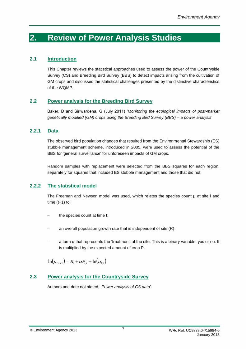
2.2.2 The statistical model

The Freeman and Newson model was used, which relates the species count μ at site i and

time (t+1) to:

the species count at time t;

an overall population growth rate that is independent of site (R);

a term α that represents the ‘treatment’ at the site. This is a binary variable: yes or no. It

is multiplied by the expected amount of crop P.

tititti PR ,,1, lnln

2.3 Power analysis for the Countryside Survey

Authors and date not stated, ‘Power analysis of CS data’.

Environment Agency



2.3.1 Data

Data from the 1998 and 2007 Countryside Surveys were used. In each survey, randomly

selected ‘X plots’ and field margin plots were surveyed within randomly selected km squares.

Species richness scores were used.

In 2007, there were 41 plots containing maize in 22 km squares, and 45 plots containing

potatoes in 22 km squares.

2.3.2 The statistical models

Two analyses were done: one purely spatial, using the 2007 data, and one using both the

1998 and 2007 surveys.

For the spatial analysis, random selections from the plots containing the relevant crop were

made, and the species richness was modified at these plots. Log linear models with a gamma

error distribution were used:

ln(species richness) ~ Overall mean + GM effect + Random effect for squares

For the temporal analysis, the difference between species richness in 2007 and 1998 was

modelled using a similar formula.

ln(species richness, 2007) ~ Overall mean + ln(species richness, 1998) + GM effect +

Random effect for squares

2.4 Generic power analysis model

CEH (2012), ‘Determining and increasing the sensitivity of existing environmental surveillance

monitoring networks…’, CB0304 Final Report

This report describes the development of a generic method of carrying out power analysis,

based on a Quasi-Poisson model for annual species counts (Freeman and Newson, 2008).

The method was used to examine the sensitivity of the power to nine factors (CB0304 table

3). There are two stages to the Monte Carlo simulation:

to generate 1000 sets of values of the nine factors;

to generate 2000 sets of species count data for each set of values of the 9 factors.

The authors then considered where the three ESNs lie on the power graphs generated by the

generic model. They also considered a data set from 34 km squares in the Countryside

Survey, where the quality (ASPT) of headwater streams was recorded using macro-

invertebrates.

Environment Agency



2.5 Power analysis for the Water Quality Monitoring Programme

Table 2.1 contrasts the WQMP with the other three ESNs analysed for their potential use in

general surveillance of GM crops.

Table 2.1 Comparison of Environmental Surveillance Networks

Aspect of

monitoring

network

Breeding Bird

Survey

Butterfly

Monitoring

Scheme

Countryside

Survey

Water Quality

Monitoring

Programme

Number of

monitoring sites

2000 nationally

but fewer for

individual

species with

restricted

distributions

(377 for reed

bunting, 704 for

Linnet)

Only ~30 sites

cross

agricultural

land

Maize: 41 plots

in 21 1x1km

squares

Potatoes: 45

plots in 22 km

squares

Too few sugar

beet plots for

analysis.

ca. 5000 sites

nationally; ca.

1700 in main

areas of maize,

sugar beet and

potatoes

cultivation (but

with variable

data quality and

significant spatial

redundancy)

Parameters

measured and

selected as

potentially useful

Yellowhammer,

Linnet and

Reed Bunting

populations

Species

counts: Small

Tortoiseshell &

Large White

Species

richness. Also

weed

abundance, soil

quality and river

macro-

invertebrates

Concentrations

of nitrate,

orthophosphate

and suspended

solids

Area represented

by each monitoring

site

Two parallel

1km transects,

each in 5 equal

sections

Fixed line

transects of 5

m width and

approximately

3 km length

Randomly

selected X plots

and arable field

margin plots, in

1 km squares.

The catchment

area upstream of

each monitoring

site ranges from

<1 to >100 km2.

Monitoring duration Began 1994.

Useful data

from 2002

onwards

Began 1976 Began 1978 -

only 2007

survey data

analysed

~10 years

Environment Agency



Aspect of

monitoring

network

Breeding Bird

Survey

Butterfly

Monitoring

Scheme

Countryside

Survey

Water Quality

Monitoring

Programme

Monitoring

frequency

Surveys

conducted

twice a year,

but not all

squares are

monitored each

year

26 weekly

counts every

year

Approx. every 7

years.

Typically

monthly (but with

occasional gaps

or additional

sampling)

The WQMP has a number of distinctive features which demand a different approach to

analysing power from that adopted for the other ESNs. In particular:

The WQMP measures physico-chemical parameters, in contrast to species counts and

richness for the other networks. A Poisson error distribution is therefore not

appropriate. After examination of residual plots, and in line with past experience, the

nitrate, orthophosphate and suspended solids concentrations were assumed to have

Log-Normal distributions and were log-transformed prior to analysis.

The CS is undertaken every 7 years and the BBS is undertaken every six months.

Because these sampling frequencies are relatively low, the CS and BBS analyses

compared samples taken from different areas with differing levels of GM uptake, at

single points in time (i.e. a spatial analysis). By contrast, the WQMP samples water

quality at roughly monthly intervals, yielding an extended time series for each

monitoring site. Attempts to detect impacts arising from GM crops therefore focus on

modelling changes in mean water quality through time (i.e. a temporal comparison of

water quality before and after the introduction of the GM crop), rather than analysing

spatial patterns in water quality among sites.

Temporal changes in water quality are known to be influenced by long-term trends in

pollutant pressure, season and rainfall, and these variables can be included in the

model as covariates to reduce the amount of unexplained variation in the data and so

help isolate and detect the impacts arising from GM crops. In contrast to the Freeman

and Newson approach, which models population change between one year and the

next, we have assumed that successive water quality measurements are not temporally

auto-correlated after accounting for the effects of time, season and rainfall.

The CS, BBS and BMS surveys take measurements from relatively small squares/plots

that are geographically separated and which can therefore be assumed to be more or

less spatially independent. By contrast, the WQMP has a relatively high density of

monitoring sites and sites in the same catchment are inherently linked by the

downstream flow of water. The complex hierarchical structure of river catchments

Environment Agency



makes this spatial autocorrelation difficult to model, so we have instead sought to

minimise the degree of autocorrelation by analysing no more than one monitoring site

from each river water body.

The relatively small plots surveyed by the CS and BMS surveys mean that the crops

within each area can reasonably be categorised as exclusively GM or not. This

facilitates the detection of GM impacts because it is possible then to directly contrast

the two extreme situations. By contrast, relatively large areas of land drain to each

WQMP monitoring site, and the area of maize, potatoes or sugar beet rarely exceeds

10% of the catchment area. Any impact of GM crops on water quality is therefore

diluted at a catchment scale and correspondingly harder to detect.

The influence of GM uptake on power was investigated for the BBS and BMS by

varying the proportion of monitoring sites with GM variety. By contrast, the WQMP

power analysis investigated the influence of GM uptake by varying the proportion of the

crop that had switched to the GM variety.

In line with the other power analyses, we assumed that the impact of the GM variety

was proportional to its coverage (i.e. the relative impact of each hectare of GM crops

was the same everywhere).

Environment Agency



Environment Agency



3. Methodology

3.1 Overview of approach

This Chapter describes the methodology used to assess the power of the WQMP, in

particular: the approach taken to selecting and processing data; the statistical model used to

detect GM crop impacts; the conceptual model used to define GM crop impacts; and the

stochastic simulation used to quantify power under a range of scenarios.

In summary, the methodology can be broken down into four main stages:

1. Maize, potatoes and sugar beet are grown only in restricted parts of England, so we

first identified water quality monitoring sites in the main areas of cultivation. Data quality

criteria were then applied to identify a subset of monitoring sites that had a reasonably

complete 10-year time series of water quality measurements.

2. A mixed-effects model was fitted to the data to characterise the temporal variation in

water quality at these sites. Time, day of the year and rainfall were included as

explanatory variables to minimise the unexplained variation and help reveal any

changes in water quality arising from cultivation of GM crops. The coefficients from the

model were then used to stochastically simulate 500 replicate time series with the same

properties as the original data.

3. The synthetic data was then modified by the inclusion of a specified GM crop impact

proportional to the coverage of that crop upstream of each site.

4. The 500 replicate time series were then analysed using the same mixed-effects model

as before, but with an additional term representing the GM crop impact. The proportion

of the time series yielding a statistically significant GM crop effect was taken to indicate

the power of the test. The simulation was then repeated for a range of scenarios to

examine how power changes with key factors such as the level of GM uptake, duration

of monitoring and number of sites.

Sections 3.2 to 3.5 explain each of these four stages in further detail.

3.2 Data selection and data processing

3.2.1 Water quality data

Three determinands were selected from the range of physico-chemical parameters monitored:

nitrate, orthophosphate and suspended solids (SS).

Environment Agency



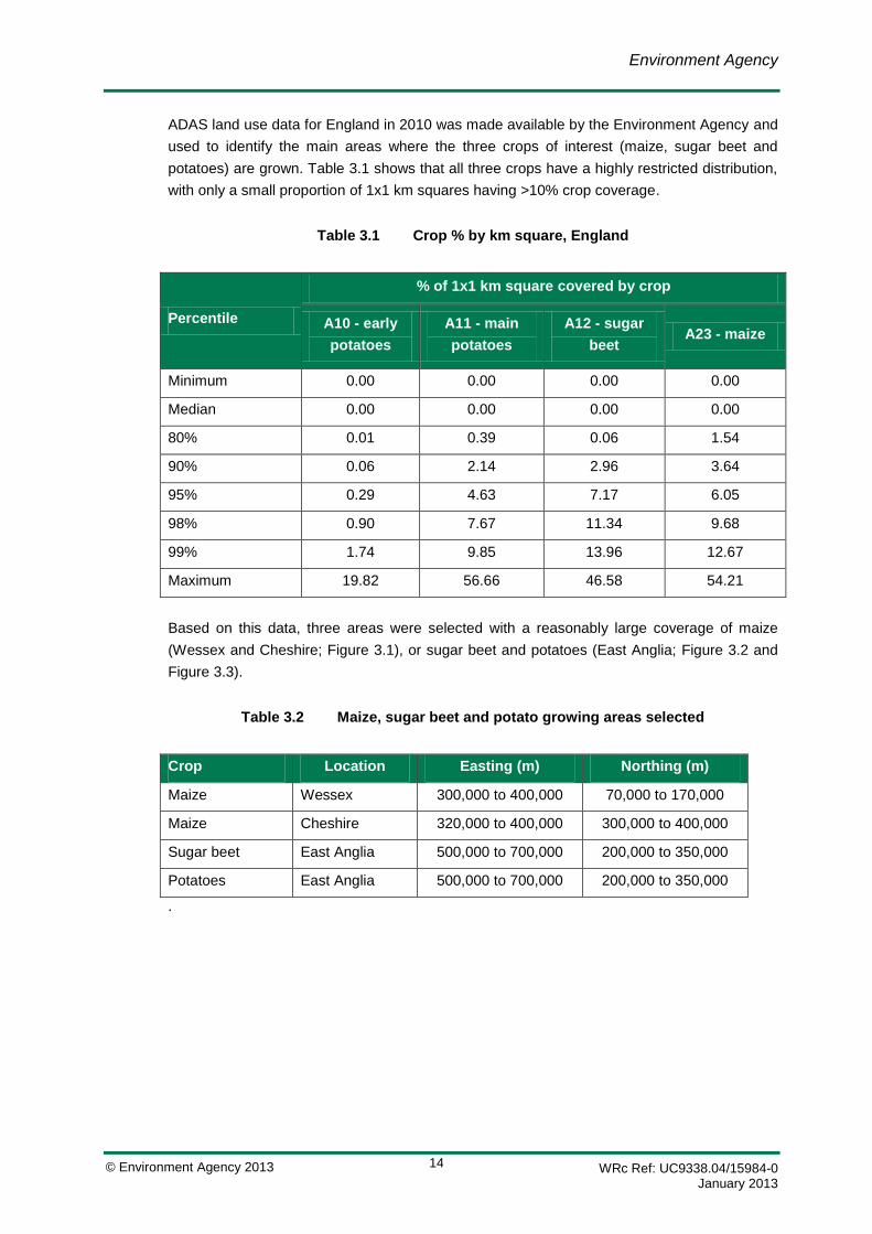
ADAS land use data for England in 2010 was made available by the Environment Agency and

used to identify the main areas where the three crops of interest (maize, sugar beet and

potatoes) are grown. Table 3.1 shows that all three crops have a highly restricted distribution,

with only a small proportion of 1x1 km squares having >10% crop coverage.

Table 3.1 Crop % by km square, England

Percentile

% of 1x1 km square covered by crop

A10 - early

potatoes

A11 - main

potatoes

A12 - sugar

beet A23 - maize

Minimum 0.00 0.00 0.00 0.00

Median 0.00 0.00 0.00 0.00

80% 0.01 0.39 0.06 1.54

90% 0.06 2.14 2.96 3.64

95% 0.29 4.63 7.17 6.05

98% 0.90 7.67 11.34 9.68

99% 1.74 9.85 13.96 12.67

Maximum 19.82 56.66 46.58 54.21

Based on this data, three areas were selected with a reasonably large coverage of maize

(Wessex and Cheshire; Figure 3.1), or sugar beet and potatoes (East Anglia; Figure 3.2 and

Figure 3.3).

Table 3.2 Maize, sugar beet and potato growing areas selected

Crop Location Easting (m) Northing (m)

Maize Wessex 300,000 to 400,000 70,000 to 170,000

Maize Cheshire 320,000 to 400,000 300,000 to 400,000

Sugar beet East Anglia 500,000 to 700,000 200,000 to 350,000

Potatoes East Anglia 500,000 to 700,000 200,000 to 350,000

.

Environment Agency



Figure 3.1 Distribution of maize in England

Figure 3.2 Distribution of sugar beet in East Anglia

Environment Agency



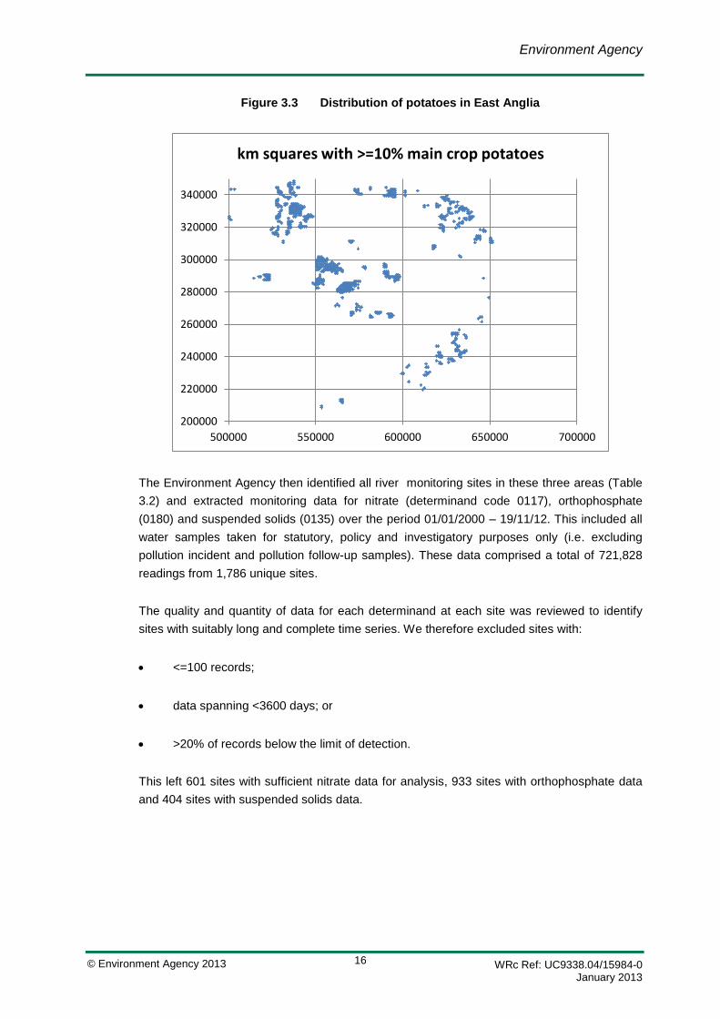
Figure 3.3 Distribution of potatoes in East Anglia

200000

220000

240000

260000

280000

300000

320000

340000

500000 550000 600000 650000 700000

km squares with >=10% main crop potatoes

The Environment Agency then identified all river monitoring sites in these three areas (Table

3.2) and extracted monitoring data for nitrate (determinand code 0117), orthophosphate

(0180) and suspended solids (0135) over the period 01/01/2000 – 19/11/12. This included all

water samples taken for statutory, policy and investigatory purposes only (i.e. excluding

pollution incident and pollution follow-up samples). These data comprised a total of 721,828

readings from 1,786 unique sites.

The quality and quantity of data for each determinand at each site was reviewed to identify

sites with suitably long and complete time series. We therefore excluded sites with:

<=100 records;

data spanning <3600 days; or

>20% of records below the limit of detection.

This left 601 sites with sufficient nitrate data for analysis, 933 sites with orthophosphate data

and 404 sites with suspended solids data.

Environment Agency



To reduce the degree of spatial auto-correlation among sites, we selected one monitoring site

per water body 1 and assumed that sites in different water bodies were spatially independent.

Whilst this is a questionable assumption (water quality at a downstream site will always be

correlated to some extent with that at upstream sites) a more sophisticated analysis of the

complex hierarchical structure of water bodies, sub-catchments and catchments was not

possible within the scope of the project. This left 190 sites with sufficient nitrate data for

analysis.

3.2.2 Land use data

The ADAS land use data was analysed in GIS to estimate the percentage cover of each crop

in each Water Framework Directive water body. Each water quality monitoring site was then

linked to its respective water body. For those monitoring sites on the main stem of the river,

the land use in that water body and all upstream water bodies was aggregated together to

estimate the percentage cover of each crop in the upstream catchment area. For those

monitoring sites not on the main stem (i.e. those on a local tributary stream that doesn’t

extend beyond the water body), the percentage cover of each crop was estimated from the

land use in just that one water body.

3.2.3 Rainfall data

To be able to model the influence of rainfall on water quality, monthly rainfall time series were

obtained from the Met Office 2 for three weather stations, one in each of the three regions:

Cambridge (to represent East Anglia), Shawbury (Cheshire) and Yeovilton (Wessex).

3.3 Statistical modelling

Exploratory analysis of the data showed there was a statistically significant relationship at

most of the selected sites between mean water quality and the following factors:

monthly rainfall;

season; and,

time.

Seasonal variation was represented by first-order Fourier series harmonics based on the day

of the year (1 – 365) and long-term time trends were modelled as a simple linear trend over

the course of the entire time series.

1 Water bodies are the basic management unit in river basin management plans. They are sections of

reasonably homogeneous river varying in length from ca. 5 km to >25 km.

2 http://www.metoffice.gov.uk/climate/uk/stationdata/

http://www.metoffice.gov.uk/climate/uk/stationdata/

Environment Agency



Due to the anticipated spatial variation in the data, a linear mixed model was chosen. Such

models enable the data to be grouped, in this case by site, and allow some of the terms in the

model to vary between groups. It was decided that the long-term trend term would be allowed

to vary randomly by site but the monthly rainfall and seasonal terms were held fixed. This

model was fitted to the data (nitrate, orthophosphate and suspended solids separately) and

was of the following form:

where:

= measured concentration at site i at time t;

= long term trend for site i at time t;

= monthly rainfall for site i at time t;

, = first-order Fourier series harmonics for site i at time t such

that d = day of year;

= random error term for site i at time t such that ;

= random effects for site i; and,

= fixed effects for all sites.

Fourier series harmonics were used in preference to a smooth term because this facilitated

analysis using a conventional (rather than additive) mixed model.

Autocorrelation plots were examined to check for temporally correlated residuals (Appendix

A). Although there was still some autocorrelation, we believe that this had a negligible effect

upon the standard errors and p-values from the model.

Once the model had been fitted to the data, it was used to stochastically generate 500

replicate time series of water quality data for each site. These 500 synthetic datasets were

then used to investigate the power of a linear mixed model to detect changes in mean water

quality arising from GM crops. In an ideal world we would have used more than 500

replicates, but this was not possible due to the timescales involved. We are confident,

however, that 500 replicates provides a reasonably stable estimate of statistical power.

Imprecision is always greatest when power = 0.5, but with 500 replicates we expect, on the

Environment Agency



basis of binomial probability theory, power to be estimated to within ±0.04 with 90%

confidence.

3.4 Conceptual model of GM crop impacts

The impact of the GM crop on water quality at a specific site was expressed as follows:

where:

= the proportional increase in pollutant concentration caused by the GM crop;

= the unit impact of GM variety;

= the uptake of the GM variety, expressed at the proportion of the crop converting to

GM: and,

= the coverage of the crop, expressed as the proportion of the upstream land area on

which the crop is grown.

The unit impact parameter ( ) can be thought of as the proportional increase in pollutant loss

from land changing to the GM variety. Making the assumption that the crop contributes

proportionately to the pollution in the river (e.g. maize covers 20% of the catchment and

contributes 20% of the nitrate load), then = 0 means that switching to the GM variety causes

no change in pollutant loss, = 0.5 means that switching to the GM variety increases pollutant

loss by 50%, = 1 means that switching to the GM variety increases pollutant loss by 100%,

and so on.

If the crop contributes disproportionately to the pollution in the river (e.g. maize covers 20% of

the catchment but contributes 40% of the nitrate load), then will take higher values to

represent the relative importance of agricultural and non-agricultural sources of pollution

within the catchment.

The synthetic datasets were then modified by adjusting the observed concentration

measurements by . We assumed that the GM variety was introduced half way through the

period of monitoring and had caused an instantaneous step change increase in mean

pollutant concentration. Note that this representation of GM impacts makes the following

assumptions:

Environment Agency



1. GM crops are taken up evenly in every catchment, so that a constant proportion (U) of

the crop converts to the GM variety everywhere.

2. The GM crop has a constant unit impact on water quality. In other words the GM variety

increases the pollutant load from each hectare by the same amount regardless of

location.

3. The GM crop has a constant proportional impact on water quality throughout the year,

not just during the growing season.

3.5 Power analysis

After modifying the synthetic datasets to include a specified GM crop impact (Section 3.4), the

500 replicate datasets were analysed using the same linear mixed model described in Section

3.3 but with an additional fixed term to measure the relationship between F and mean water

quality:

The percentage of the 500 synthetic datasets that yielded a statistically significant (at α =

0.05) coefficient for F (β5) was interpreted as a measure of the power of the model to detect

the GM crop impact specified by and .

This process was repeated with different parameter settings to explore how power varies with

GM uptake, GM crop impact, duration of monitoring and number of monitoring sites (Table

3.3).

Table 3.3 Scenarios used in the power analysis

Parameter Description Range of values examined

The level of GM

uptake ( )

Expressed as the proportion of crop

converting to GM

0.25, 0.5, 0.75 and 1.0

The unit impact of

GM variety ( )

Expressed as the proportional increase

in pollutant loss, relative to the

conventional variety

From 0.1 to 2.0

The duration of

monitoring

Data was synthesised for a 10 (2002 to

2011) or 20 (1992 to 2011) year period

using actual rainfall data

10 and 20 years

The number of

monitoring sites

The network of 190 sites was halved by

selecting alternate sites listed

alphabetically, and doubled by

duplicating each site

95, 190 and 380 sites (for

nitrate)

Environment Agency



4. Results

This chapter presents the results of the power analysis, focusing on how power changes with

the scale of GM crop uptake, the degree of GM crop impact, the number of years of

monitoring data and the number of monitoring sites.

4.1 Power to detect impacts of GM maize on nitrate

Due to time constraints, the methodology described in Chapter 3 was used to quantify the

power to detect changes in mean nitrate concentration arising from GM maize. The

applicability of these results to the other crops and other water quality determinands is

discussed in Section 4.2.

4.1.1 Effect of GM uptake and GM impact

Figure 4.1 shows how the power to detect change over a 10 year period (5 years of data

before and 5 years of data after the introduction of the GM variety) varies with the level of

uptake (U) and the unit impact of GM variety ( ). Power is high (>0.8) if all the maize is GM

(U =1) and the GM variety increases losses of nitrate by at least 50% ( >=0.5). At lower

levels of uptake (U <= 0.50), only very large increases in nitrate loss ( >=1.0) will have a high

chance of being detected. This scenario (i.e. using 10 years of data and 190 sites) is used a

reference for comparison in the following sections as the length of the monitoring period and

number of sites are altered and the effect on power explored.

Figure 4.1 Power for a range of values of γ and U for a 10 year time period using 190

sites

0.0 0.5 1.0 1.5 2.0

0.0

0.4

0.8

Unit impact of GM crop

po

we

r

Uptake = 0.25

Uptake = 0.5

Uptake = 0.75

Uptake = 1

Environment Agency



4.1.2 Effect of the length of monitoring period

Figure 4.2 shows the same graph as in Figure 4.1 and compares this with power results from

an identical analysis but using 20 years of monitoring data (10 years of data before and 10

years of data after the introduction of the GM variety) instead of 10 years. It can be seen that

for all levels of uptake considered, power increases when a longer monitoring period is used.

Power is then high (>0.8) if most of the maize is GM (U > 0.5) and the GM variety increases

losses of nitrate by at least 40% ( >=0.4).

Figure 4.2 Power for a range of values of γ and U for a 10 year time period and a 20

year time period using 190 sites

0.0 0.5 1.0 1.5 2.0

0.0

0.4

0.8

10 years


po

we

r

Uptake = 0.25

Uptake = 0.5

Uptake = 0.75

Uptake = 1

0.0 0.5 1.0 1.5 2.0

0.0

0.4

0.8

20 years


po

we

r

Uptake = 0.25

Uptake = 0.5

Uptake = 0.75

Uptake = 1

Environment Agency



4.1.3 Effect of number of sites

Figure 4.3 shows the same graph as in Figure 4.1 and compares this with power results from

an identical analysis but using firstly half the number of monitoring sites (95 sites as opposed

to 190) and secondly double the number of monitoring sites (380 sites). It can be seen that for

all levels of uptake considered, power worsens as the number of sites used decreases. On

the other hand, power increases as the number of sites increases.

When using only 95 sites, power is high (>0.8) if all the maize is GM (U = 1.0) and the GM

variety increases losses of nitrate by at least 70% ( >=0.7). It can also be seen that when

only 25% of the maize is GM (U=0.25), the power does not reach 50% even when the GM

variety increases losses of nitrate by 200% ( =2.0).

When using 380 sites, power is high (>0.8) if most of the maize is GM (U > 0.5) and the GM

variety increases losses of nitrate by at least 40% ( >=0.4). The effect of increasing the

number of sites used is therefore similar to the effect of increasing the length of the monitoring

period.

Environment Agency



Figure 4.3 Power for a range of values of γ and U for a 10 year time period using 95

sites, 190 sites and 380 sites

0.0 0.5 1.0 1.5 2.0

0.0

0.4

0.8

95 sites


po

we

r

Uptake = 0.25

Uptake = 0.5

Uptake = 0.75

Uptake = 1

0.0 0.5 1.0 1.5 2.0

0.0

0.4

0.8

190 sites


po

we

r

Uptake = 0.25

Uptake = 0.5

Uptake = 0.75

Uptake = 1

0.0 0.5 1.0 1.5 2.0

0.0

0.4

0.8

380 sites


po

we

r

Uptake = 0.25

Uptake = 0.5

Uptake = 0.75

Uptake = 1

Environment Agency



4.2 Power to detect other GM crop impacts

Section 4.1 quantifies the power of the WQMP to detect changes in mean nitrate

concentration arising from GM maize. Due to time constraints it was not possible to compare

the power to detect impacts arising from maize, sugar beet and potatoes, or to compare the

power to detect impacts on nitrate, orthophosphate and suspended solids. We have

reasonable grounds for believing, however, that the maize-nitrate combination represents a

‘best case’ situation and that power will be similar or lower for other crops and other

determinands.

4.2.1 Comparison of crop types

Maize is most commonly grown crop, being present in over 20% of 1x1 km squares in

England (Table 3.1), and so potentially affects the largest number of monitoring sites. Maize

also has a restricted distribution, being concentrated in Wessex and Cheshire, so any water

quality impacts will tend to be concentrated in these areas.

Sugar beet cultivation is largely restricted to East Anglia, so the number of affected

monitoring sites is lower, but any impacts are likely to be more pronounced because of the

relatively high concentration of sugar beet crops. We therefore expect the power to detect

impacts from sugar beet to be similar to those for maize (all else being equal).

Potato cultivation is spatially restricted but locally concentrated. We therefore expect the

power to detect impacts from potatoes to be considerably lower than for maize and sugar beet

(all else being equal).

4.2.2 Comparison of water quality determinands

Nitrate has the lowest temporal variation in concentration of the three determinands

examined; of the 1,786 monitoring sites examined in this study, the average coefficient of

variation was 0.38. Nitrate also tends to exhibit relatively clear seasonal patterns, with the

highest concentrations in winter and lowest in summer. This means that the residual error

variance (i.e. the within-site variability left after accounting for long-term trends, seasonality

and rainfall) is relatively low and less likely to mask increases in mean concentration caused

by the cultivation of GM crops. Nitrate is widely monitored and over 600 sites had sufficient

nitrate data for analysis.

Orthophosphate shows higher temporal variation in concentration than nitrate; of the 1,786

monitoring sites examined in this study, the average coefficient of variation was 0.80. It is very

widely monitored, however, with over 900 sites having sufficient data for analysis. We

therefore expect the power to detect GM crop impacts on orthophosphate to be slightly lower

than for nitrate (all else being equal).

Environment Agency



Suspended solids has the highest temporal variation in concentration of the three

determinands examined; of the 1,786 monitoring sites examined in this study, the average

coefficient of variation was 1.49. It is also widely monitored, but after data cleaning only 400

sites had sufficient data for analysis. We therefore expect the power to detect GM crop

impacts on suspended solids to be considerably lower than for nitrate (all else being equal).

Environment Agency



5. Discussion and Conclusions

This chapter discusses the potential of the WQMP to detect GM crop impacts on water

quality, draws comparisons with the other ACRE-commissioned power analyses, discusses

the limitations of the power analysis, and makes recommendations for improving the power of

the WQMP.

5.1 Can GM impacts on water quality be detected?

The results of this study suggest that the existing WQMP can detect adverse impacts of GM

crops on water quality, but that power will be high (> 0.8) only if (i) GM crops are widely

adopted (uptake is at least 75%), (ii) GM varieties were to cause a large (>= 50%) increase in

pollutant losses relative to conventional varieties, and (iii) at least 10 years of monitoring data

is available from several hundred affected monitoring sites.

This finding is broadly consistent with those reported by other ACRE-commissioned power

analyses, which found that ESNs such as the CS and BBS could be used to detect

unanticipated effects resulting from the cultivation of GM crops but that the uptake of GM

crops will need to be quite extensive and the local biological effects quite significant before

effects are detectable.

Relative to other ESNs, the WQMP has a high number of monitoring sites and a high

frequency of sampling, and so generates a very large volume of data with which to analyse

GM crop impacts. On the other hand, individual crop types (maize, sugar beet and potatoes)

rarely cover more than 10% of a catchment’s area, and more typically cover just 1 - 5%. This

means that GM crops can have a pronounced effect on pollutant losses at the field scale and

yet have an only minor impact on water quality at a catchment scale. As the WQMP measures

water quality at a sub-catchment scale, power to detect changes in water quality can be low.

By contrast, the relatively small plots surveyed by the CS, and BBS surveys can have very

high levels of GM crop coverage, and the localised impacts of those crops can be very

pronounced and easier to detect.

5.2 Limitations of the power analysis

The power analysis undertaken for the WQMP necessarily makes a number of simplifying

assumptions about the future uptake and impact of GM crops. It was not possible, within the

constraints of this project, to formally examine the influence of all these assumptions, but it is

nonetheless possible to comment on the validity of some of the main assumptions, and

whether these assumptions are likely to over- or under-estimate the statistical power to detect

deterioration in water quality.

Environment Agency



We assumed that the GM variety is introduced half way through the period of

monitoring and causes an instantaneous step change increase in mean pollutant

concentration. In reality, the adoption of GM varieties is likely to be a more gradual

process and the proportion of GM varieties is likely to vary from year to year. With good

quality, up-to-date information on GM crop uptake and changing cropping patterns, we

believe that this should not significantly reduce the power to detect water quality

impacts so long as there is sufficient monitoring data after the uptake of GM crops has

stabilised.

We assumed that GM crops are taken up evenly in every catchment, so that a constant

proportion (U) of the crop converts to the GM variety everywhere. In reality uptake will

vary from farm to farm, but at larger catchment scales we expect uptake to be relatively

similar. Unless very detailed, farm-scale data on GM crop cultivation is available, we

expect this to slightly reduce the power to detect water quality impacts.

We assumed that the GM crop has a constant unit impact on water quality – i.e. that

the GM variety increases the pollutant load from each hectare by the same amount

regardless of location. Again, the unit impact will vary spatially in reality depending on

soil properties and farming practices, which will slightly reduce the power to detect

water quality impacts at a regional scale.

We assumed that monitoring sites in different water bodies were spatially independent

of each other. In reality, water quality at a downstream site will almost always be

correlated to some extent with that at upstream sites, so there will be some information

redundancy, the Type I error rate will be slightly higher than the nominal 5%, and power

will be slightly over-estimated. It is possible that the use of more sophisticated mixed

models that better portray the spatial autocorrelation between neighbouring sites may

help to overcome this shortcoming.

5.3 Options for improving power

There are at least four ways in which the power to detect water quality impacts could be

improved.

1. Refine the statistical models to reduce the residual error variation. We used monthly

rainfall as a covariate to try to explain some of the temporal variation in water quality at

each site. This proved to be a poor predictor, probably because monthly aggregated

data does not adequately reflect the frequency and severity of storm events which

strongly influence the mobilisation and transport of diffuse pollutants. Use of higher

resolution rainfall data, or other relevant covariates, could help to improve the

performance of the models used.

2. Increase the number of sites in the monitoring network. This would produce a larger

dataset and increase the chances of detecting a statistically significant GM crop impact.

Environment Agency



There will be a practical limit to the number of independent sites (i.e. sub-catchments)

that can be monitored, however, because sites in close proximity will tend to be

strongly correlated. Any new sites should therefore be located in small, sub-catchments

that are not currently monitored. For instance, there are a large number of monitoring

sites in the dataset used in this report, but the number of sites used in the analysis was

much smaller due to the need to exclude strongly correlated sites. New sites will, of

course, not have any historic monitoring data, so this strategy will only be effective if

sites can be established and accumulate measurements over a reasonable time period

before the introduction of GM crops.

3. Increase the length of the monitoring period. A longer run of pre- and post-GM

monitoring would produce a larger dataset and increase the chances of detecting a

statistically significant GM crop impact.

4. Increase the frequency of sampling at each monitoring site. This would produce a

larger dataset and potentially increase the chances of detecting a statistically significant

GM crop impact. The closer together successive samples are taken, however, the more

strongly auto-correlated the results will be, so there is a limit to how much additional

information can be gained this way.

5.4 Conclusions

In summary, the existing WQMP can detect adverse impacts of GM crops on water quality,

but power will be high only when (i) GM crops are widely adopted, (ii) GM varieties cause a

pronounced increase in pollutant losses relative to conventional varieties, and (iii) at least

10 years of pre- and post-GM monitoring data is available from several hundred affected

monitoring sites.

Existing indicators of water quality, such as the Environment Agency’s Ecological Status

Indicator (ESI), are intended to describe, quantify and test the statistical significance of

national changes in water quality. They are used primarily as a means of tracking long term

progress towards meeting national water quality targets, not for examining the causes of

observed trends. Revealing any unanticipated impacts arising from the cultivation of GM

crops in the future will therefore require a specific data analysis study using the type of

statistical modelling approach described in this report.

This basic approach of analysing data from multiple monitoring sites to test the influence of

widespread environmental impacts could, in theory, be used to examine water quality impacts

arising from other changes in land use or farming practice, or water quality improvements

arising from pollution mitigation measures.

Environment Agency



Environment Agency



Appendix A Model Checking

Autocorrelation is a key feature in time series data which must be accounted for when model

fitting. The fixed terms in the model (i.e. long-term trend, Fourier series harmonics, and

monthly rainfall) were found to remove much of the temporal correlation between successive

nitrate concentrations (Figure A.1). Although there was still some autocorrelation, we believe

that this will have a negligible effect upon the standard errors and p-values associated with

the GM impact term, and hence the estimate of power.

Figure A.1 Autocorrelation plot for linear mixed nitrate model

0 10 20 30 40

0.0

0.2

0.4

0.6

0.8

1.0

Lag

AC

F

.

power analysis of the routine water quality monitoring

Documents