poverty in iraq, 2012 - 2014 - world...

POVERTY IN IRAQ, 2012 - 2014

This note describes the methodology used for estimating trends in poverty

rates for Iraq using the 2012 Iraq Household Socio-Economic Survey and the

2014 Continuous Household Survey; and presents the findings. The 2014

survey was designed to provide comparable and more frequent estimates of

poverty, but fieldwork was disrupted in the second half of 2014 due to a

deteriorating security situation. The methodology described in this note

implements adjustments to weights and re-estimates the poverty line to

establish poverty trends between the first half of 2012 and the first half of

2014 for all 18 governorates of Iraq; between the first and second half of

2014 for 13 governorates of Iraq; and between 2012 and 2014 for these 13

governorates. The first set of estimates show that the pace of poverty

reduction in Iraq was accelerating until the first half of 2014, while the

second and third set of estimates quantify the adverse impact of the 2014

crisis on welfare in 13 governorates of Iraq.

World Bank and

Government of Iraq

and Kurdistan

Region, 2015-16

Pub

lic D

iscl

osur

e A

utho

rized

Pub

lic D

iscl

osur

e A

utho

rized

Pub

lic D

iscl

osur

e A

utho

rized

Pub

lic D

iscl

osur

e A

utho

rized

Table of Contents The 2014 Continuous Household Survey: Design and Challenges in Implementation ........................................................................... 2

Analytical Approach ........................................................................................................................................................................... 2

Pre-crisis trends in poverty: 2012 1st half and 2014 1st half, 18 governorates ......................................................................................... 3

Crisis impact: 2014 1st half and 2014 2nd half, 13 governorates............................................................................................................... 7

Poverty between 2012 and 2014: 2012 and 2014 full year,13 governorates .......................................................................................... 9

Annex 1: METHODOLOGY FOR ADJUSTING HOUSEHOLD WEIGHTS IN CONTINUOUS HOUSEHOLD SURVEY – JANUARY-MAY

2014.................................................................................................................................................................................................. 12

Background and Objective ............................................................................................................................................................ 12

Construction of weights in IHSES 2012........................................................................................................................................... 15

CHS 2014: Post-stratification of weights ........................................................................................................................................19

LIST OF TABLES

Table 1: Poverty lines – 2012 ............................................................................................................................................................... 3 Table 2: Trends in poverty 2012 (1st half) – 2014 (1st half) ..................................................................................................................... 5 Table 3: Governorate poverty rates - (1st half 2012 vs. 1st half 2014) ................................................................................................... 5 Table 4: Trends in inequality: 1st half 2014 relative to 1st half 2012 ....................................................................................................... 6 Table 5: Poverty line – 2012 based on 13 governorates ........................................................................................................................ 9 Table 6: Poverty rates in 2012 and population of reference: Whole Country vs. 13 Governorates ......................................................... 10 Table 7: Poverty rates based on 13 governorates – 2012 vs. 2014 ........................................................................................................ 11 Table 8: Households Interviewed per Month in CHS * ........................................................................................................................ 13 Table 9: Weighting Factors in CHS ..................................................................................................................................................... 14 Table 10: Weighting Factors in Urban areas for two time intervals in CHS ........................................................................................... 15 Table 11: Number of Households Interviewed per Month in IHSES 2012 ............................................................................................. 15 Table 12: Weighting Factors in IHSES 2012 ........................................................................................................................................16

LIST OF FIGURES

Figure 1: Probability density function and cumulative distribution of welfare, 1st half 2012 versus 1st half 2014 ................................... 4 Figure 2: Consumption growth incidence curve: 1st half 2014 relative to 1st half 2012 ......................................................................... 6 Figure 3: More than half of poverty reduction was due to the reduction in inequality ............................................................................ 7 Figure 4: Incidence of poverty – first and second half 2012 .................................................................................................................. 8 Figure 5: Poverty impact of the twin crises (13 governorates) .............................................................................................................. 9 Figure 6: Weighting Factors in IHSES-II and CHS in two time intervals – urban areas .......................................................................... 18 Figure 7: weighting factors in IHSES-II and CHS in two time intervals – rural areas ............................................................................. 18

1. The 2014 Continuous Household Survey: Design and Challenges in Implementation

The 2014 Continuous Household Survey (CHS) was implemented by the Central Statistics Office (CSO) of Iraq and

the Kurdistan region Statistics Office (KRSO) to provide more frequent estimates of poverty for the country. Iraq’s

national poverty estimates are currently based on two large scale surveys, the Iraq Household and Socio-Economic

Surveys (IHSES) from 2007 and 2012. These very larger and comprehensive surveys are implemented roughly every

five years, because of the costs of the survey in terms of budget but also in terms of logistical preparations and

personnel.

In order to get more frequent poverty estimates in-between IHSES years, the CHS was fielded in 2014. It was

envisaged that CHS would be implemented in between IHSES years to provide representative estimates of poverty

and a range of other socio-economic indicators at the level of governorates or provinces. The design of the CHS by

the statistical agencies in Iraq was careful and deliberate to preserve comparability. The CHS surveys a sub-sample

of IHSES clusters or PSUs, and contains a subset of IHSES modules. In particular, key modules for the construction

of a comparable welfare aggregate were identical to the IHSES – the household roster, education modules, modules

on labor market outcomes, food and non-food consumption expenditures, consumption and expenditures on

rations or PDS items, and incomes from earnings and public and private transfers. Fieldwork began in November

2013 and was supposed to run for 12 months. The intended sample of 13,834 households was drawn to be

representative at the governorate level. The sample was temporally and spatially stratified, with each month or

wave of the sample designed to be nationally representative.

However, fieldwork and data collection for the 2014 CHS was disrupted beginning in June 2014 due to the

deteriorating security situation in some areas and the growing influence of Islamic State (IS) militants in the

northwest of the country. As a result, in five governorates, fieldwork could not be completed as planned – Nineveh,

Anbar, Salahadin, Kirkuk and Baghdad. In Baghdad the last quarter was severely affected in terms of response rates,

and no household in rural Baghdad could be interviewed. In the remaining 13 governorates, fieldwork continued as

planned. In the second half of 2014, the sharp decline in oil prices also severely cut the government budget. While

this did not affect fieldwork, together, these two simultaneous and exogenous shocks in the middle of 2014 provide

a natural experiment setting for the 2014 CHS, with the first half being characterized by “normal” conditions and

the second half by crisis conditions, at least for the 13 governorates where data collection was completed as planned.

2. Analytical Approach

Despite the sudden disruption of fieldwork, the 2014 CHS contains a lot of critical information that can be revealed

by undertaking careful analysis, in large part due to the careful attention paid ex-ante to the design of the CHS.

First, it can provide a benchmark or counterfactual for the country for 2014 prior to the crisis. In other words, the

first half of the survey, covering the period until May 2014, covers all governorates in the country, and can provide

an estimate of pre-crisis welfare measures. However, there are some challenges. While the intended sample size of

households was surveyed as intended in the first half of the CHS, it was not balanced across urban and rural areas.

As a result, survey weights needed to be adjusted to redress this imbalance. The details are in Annex 1. Moreover,

in order to establish trends and comparable welfare estimates, it is necessary to identify the comparable population

in 2012. To do that, households from rural Baghdad had to be excluded from the first half of the 2012 IHSES, the

welfare aggregate needed to be re-estimated for this sample, and a consistent poverty line needed to be estimated.

Secondly, the 2014 CHS can provide an estimate of the Twin crises of Islamic State militancy and the oil price shock

on the 13 governorates for which data collection was completed. For these governorates, a comparison of first half

and second half welfare measures provides an estimate of the oil price shock impact as well as the “indirect” impact

of hosting people displaced by the IS crisis and the accompanying economic disruptions.

Thirdly, we can monitor the trend in poverty between 2012 and 2014 by considering the set of 13 governorates with

complete information in 2014. A comparison of the welfare measures provides insights both on the evolution in the

incidence of poverty and the impact of the twin crises in these governorates.

3. Pre-crisis trends in poverty: 2012 1st half and 2014 1st half, 18 governorates

The first step in estimating pre-crisis trends in poverty is to recalculate the poverty line for Iraq (excluding rural

Baghdad) based on 2012 IHSES welfare aggregates for the comparable period, i.e. January to May 2012. These are

presented in Error! Reference source not found., and as is evident, there is little indication of seasonality. The 1st

half poverty line is only slightly higher (1.1 percent) relative to that for the whole year. The welfare aggregate is then

calculated for the first half of 2014, excluding rural Baghdad, in a manner consistent with the official methodology,

then converted to 2012 prices using the inflation rate implied by the official CPI between January-May 2012 and

January-May 2014.

TABLE 1: POVERTY LINES – 2012

Period of time

Whole year 105,500.40 ID

First Half (January-May) 106,634.14 ID

Source: Staff estimates based on IHSES 2012

The results of this exercise indicate a secular improvement in welfare across the distribution, implying a reduction

in poverty for all reasonable poverty lines (Error! Reference source not found.). There was a shift to the right of

the whole per capita expenditure between the first half of 2012 and first half of 2014.

FIGURE 1: PROBABILITY DENSITY FUNCTION AND CUMULATIVE DISTRIBUTION OF WELFARE, 1ST HALF 2012 VERSUS

1ST HALF 2014

Source: Staff estimates based on IHSES 2012 and CHS 2014

In fact, there was a faster drop in poverty between the first half of 2014 relative to the 1st half of 2012 than had been

recorded during the 2007 to 2012 period. Compared to the 1st half of 2012, poverty fell by 5.7 percentage points in

the 1st half of 2014, i.e. from 17.5 percent to 11.8 percent. This reduction in poverty was experienced not only in rural

areas (a decline by 8 percentage points) but also in urban areas (a decline of 4 percentage points). The poverty gap

0

0.001

0.002

0.003

0.004

0.005

0.006

0.007

0.008

0 100 200 300 400 500 600

Pro

bab

ility

de

nsi

ty f

un

ctio

n

Per capita expenditure

2012 Median 2012 2014 Median 2014

0

0.2

0.4

0.6

0.8

1

0 100 200 300 400 500 600

Cu

mu

lati

ve d

istr

ibu

tio

n

Per capita expenditure

2012 2014

and the squared poverty gap also fell, although this decline was larger in rural areas. Overall, Iraq was on a better

trajectory than in the recent past before the crisis hit, with welfare improving across the country.

TABLE 2: TRENDS IN POVERTY 2012 (1ST HALF) – 2014 (1ST HALF)

Poverty Headcount Rate Poverty Gap Squared Poverty Gap

2012 2014 Change

2012 2014 Change

2012 2014 Change

Urban 12.0 7.8 -4.2 2.2 1.2 -1.1 0.6 0.3 -0.3

Rural 29.5 21.4 -8.1 7.5 4.7 -2.8 2.7 1.5 -1.2


Governorate level estimates and trends in poverty should be interpreted with caution because the lower sample

sizes imply that not all changes are significantly different at standard confidence intervals. However, in five

governorates, we can be confident of significant declines in poverty – these are Anbar, urban Baghdad, Missan, Thi

Qar and Wasit (in bold, Error! Reference source not found.).

TABLE 3: GOVERNORATE POVERTY RATES - (1ST HALF 2012 VS. 1ST HALF 2014)

2012 2014 Change

Duhouk 5.0 6.6 1.6

Nineveh 30.3 19.9 -10.4

Suleimaniya 2.4 0.9 -1.5

Kirkuk 7.2 4.6 -2.6

Erbil 3.3 1.7 -1.7

Diyala 17.0 19.0 2.0

Al-Anbar* 17.4 7.7 -9.7

Baghdad* 9.0 1.6 -7.4

Babil 17.9 13.5 -4.5

Kerbala 8.8 5.1 -3.8

Wasit* 27.9 11.5 -16.4

Salahuddin 20.1 9.7 -10.3

Al-Najaf 7.7 14.6 6.9

Al-Qadisiya 38.4 26.1 -12.3

Al-Muthanna 39.8 49.0 9.1

Thi-Qar* 45.6 17.2 -28.4

Missan* 40.7 21.4 -19.3

Basrah 18.7 22.7 4.0

Iraq* 17.5 11.8 -5.7

Note: * indicates significant changes Source: Staff estimates based on IHSES 2012 and CHS 2014

This large improvement in welfare reflects a shift in how the consumption distribution was growing, from pro-rich

growth in 2012 to pro-poor growth in the first half of 2014 (Error! Reference source not found.). Per capita

consumption grew much faster for the lower deciles of the distribution – as high as 8 to 10 percent per year in the

bottom 2 deciles. This has also implied a decline in consumption inequality, especially in rural areas, where the Gini

coefficient fell by 2.5 percentage points (Error! Reference source not found.).

FIGURE 2: CONSUMPTION GROWTH INCIDENCE CURVE: 1ST HALF 2014 RELATIVE TO 1ST HALF 2012

TABLE 4: TRENDS IN INEQUALITY: 1ST HALF 2014 RELATIVE TO 1ST HALF 2012

2012 2014 Change

Theil Gini Theil Gini Theil Gini

Total 15.5 29.9 14.8 28.9 -0.7 -0.9

Urban 14.5 29.1 14.6 28.8 0.1 -0.3

Rural 13.9 27.9 11.1 25.4 -2.9 -2.5


-4

-2

0

2

4

6

8

10

12

14

16

0 10 20 30 40 50 60 70 80 90 100

An

nu

al g

row

th r

ate,

%

Expenditure percentiles

These higher rates of consumption

growth and the reduction in

inequality (or the redistribution

effect) both contributed almost

equally to poverty reduction in the 1st

half of 2014 (Figure 3). This is in

contrast to 2012, where

redistribution worked against

poverty reduction.

4. Crisis impact: 2014 1st half and 2014 2nd half, 13 governorates

Except for five governorates (i.e. Anbar, Kirkuk, Nineveh, Salahadin, Baghdad), 2014 CHS data collection was

completed as intended. For these governorates, the first half of the year represents a ‘Business As Usual’ case; the

second half incorporates the impact of the Twin Crises.

How can the impact of the Twin Crisis be measured? If there are no systematic differences between the first half of

the year and the second half of the year other than the shocks associated with the Twin Crisis, for instance, because

of differences in seasons or festivals such as Eid, then we can be fairly confident that the differences in measured

welfare are due to the shocks. To adopt this before and after approach, we need to first test whether Iraq’s

consumption data exhibits differences across the first and second half of the year, during “normal” years. If there

are measurable differences, then we would need to adjust the estimates of crisis impact by the seasonality effect.

2012 IHSES data suggests there is no seasonal effect across the first and second half of the year in “normal” years.

The difference between first half and second half 2012 poverty lines is less than 0.5 percent, and there is no

significant difference in estimates of poverty incidence, gap and severity (Figure 4). This suggest that a comparison

of 2014 first and second half estimates will not be affected by seasonality but will rather measure differences due

to the Twin Crises.

FIGURE 3: MORE THAN HALF OF POVERTY REDUCTION WAS DUE TO THE

REDUCTION IN INEQUALITY


-2.4

-3.0

-6.0

-4.0

-2.0

0.0

FIGURE 4: INCIDENCE OF POVERTY – FIRST AND SECOND HALF 20121


Relative to the first half of 2014, poverty in Iraq (excluding the five IS-affected governorates where fieldwork was

disrupted), increased 3 percentage points by the second half of 2014, from 12.9 percent to 15.8 percent (Figure 5).

This was driven by significant increases in headcount rates in Kurdistan and the South. In Kurdistan, the Twin Crises

increased poverty estimates from 1.5 percent to 6 percent; whereas in the South, poverty increased from 22 percent

to 26.4 percent. These trends were accompanied by an increase in the poverty gap in Kurdistan region. In the South,

the increase in poverty is likely to be driven by the decline in oil prices, whereas in Kurdistan, it is also due to the

influx of displaced persons from the rest of Iraq. These estimates are based on households who were included in the

sample of the 2014 CHS, so it is important to note that they do not include internally displaced persons, and are

therefore, an underestimate of poverty headcount rates of current residents in these parts of the country.

1 Kurdistan: Duhok, Sulaimaniya and Erbil; South: Qadisiya, Muthanna, Thi-Qar, Maysan and Basrah; Rest of the North: Diyala,

Salahadin; Centre: Babylon, Kerbela, Wasit and Najaf

0.0

5.0

10.0

15.0

20.0

25.0

30.0

35.0

40.0

1st 2nd 1st 2nd 1st 2nd 1st 2nd 1st 2nd

Iraq Kurdistan Rest of North Centre South

FIGURE 5: POVERTY IMPACT OF THE TWIN CRISES (13 GOVERNORATES)

Source: Staff estimates estimations based on IHSES 2012 and CHS 2014

5. Poverty between 2012 and 2014: 2012 and 2014 full year, 13 governorates

Another option for monitoring welfare and poverty over the 2012 to 2014 period is to restrict attention to the set of

13 governorates where complete data is available, considering them together as a “country”. To undertake such a

comparison, a re-estimation of the real consumption aggregate is necessary based on a proper temporal and spatial

adjustment in 2014. For comparability reasons over time, these same adjustments have to be implemented in 2012.

This task comprises not only the recalculation of the real consumption measure but also the poverty line.

The population under analysis in IHSES 2012 includes only households that lived in the same set of 13 governorates

mentioned above. The resulting dataset covers 16,735 out of 24,944 total households in IHSES 2012. As the

population changes, households’ expenditures need to be recalculated using temporal deflators that take into

account the average CPI in this subset of governorates. These expenditures are then spatially adjusted to account

for relative price differences in the 13 governorates. The final step is to estimate a poverty line based on this subset

of spatially-adjusted expenditures.

The value of the poverty line estimated for the 13 governorates is close to the one estimated based on the whole

country (105,500.00 ID) but not exactly the same – precisely, it is 3.1% lower. This should not be surprising, as the

population of reference now excludes Baghdad, which accounts for about one fifth of the population and is

characterized by relatively high expenditures per capita.

TABLE 5: POVERTY LINE – 2012 BASED ON 13 GOVERNORATES

Whole year 102,349.00 ID

Source: Own estimation based on IHSES 2012

It is important to highlight here that there are differences between estimates for 2012 based on the whole country

and estimates for 2012 based on 13 governorates. Even though these differences are not statistically significant

from zero for all governorates except for Missan, there are some reasons why these are not exactly the same.

12.915.8

1.5

6.0

16.7

11.4 10.7 10.7

21.9

26.4

0.0

5.0

10.0

15.0

20.0

25.0

30.0

35.0

1st 2nd 1st 2nd 1st 2nd 1st 2nd 1st 2nd

Iraq Kurdistan Rest of North Centre South

The values of the Paasche index used to spatially-adjust the per capita expenditures depend on the relative prices

in the population of reference. As the population under analysis is now composed of 13 governorates instead of the

whole country, the values of the adjustment factor change and consequently the spatially-adjusted expenditures.

In particular, the exclusion of Baghdad significantly altered the structure of the relative prices. The re-estimated

expenditures are the basis of a new poverty line and the combined effect can determine a change in the levels of

poverty. The results of this re-estimation for 2012 are shown in Table 6.

TABLE 6: POVERTY RATES IN 2012 AND POPULATION OF REFERENCE: WHOLE COUNTRY VS. 13 GOVERNORATES

2012 Complete Country 2012 (13 governorates)

Estimate Std. Err. [95% Conf. Interval] Estimate Std. Err. [95% Conf. Interval]

Duhouk 6.2 0.8 4.6 7.8 6.1 0.8 4.4 7.7

Suleimaniya 2.1 0.3 1.6 2.7 2.1 0.3 1.5 2.6

Erbil 4.3 0.7 2.9 5.7 4.4 0.7 3 5.7

Diyala 20.7 1.4 18.0 23.5 19.8 1.4 17.1 22.6

Babil 14.8 1.4 12.1 17.6 13.8 1.4 11.1 16.5

Kerbala 13.1 1.9 9.3 16.8 12.6 1.9 8.9 16.3

Wasit 26.8 1.8 23.3 30.3 25.9 1.8 22.4 29.3

Al-Najaf 10.6 1.7 7.2 14.0 9.9 1.7 6.6 13.2

Al-Qadisiya 45.1 2.1 41.1 49.2 44.1 2.1 40.1 48.2

Al-Muthanna

52.6 2.3 48.0 57.1 50.9 2.3 46.3 55.5

Thi-Qar 40.9 1.9 37.3 44.6 41.7 1.9 38.1 45.4

Missan 42.5 2.1 38.3 46.7 50.1 2.2 45.9 54.4

Basrah 14.6 1.4 11.8 17.3 15.7 1.5 12.8 18.6

Iraq 19.1 0.4 18.3 19.9 20.4 0.5 19.5 21.3


Table 7 presents the estimates based on the comparison of these 13 governorates in 2012 and 2014 using the full

year sample. 8 out of 13 governorates had a significant change (i.e. positive or negative) in the headcount rate.

Duhouk and Basrah experienced an increase in their incidence of poverty of almost 6 and 7.5 percentage points.

The other 5 governorates experienced a decline in poverty rates of less than 3 percentage points in Erbil to more

than 20 percentage points in Thi-Qar and Qadisiya. The remaining 5 governorates had no significant changes in

their headcount levels.

TABLE 7: POVERTY RATES BASED ON 13 GOVERNORATES – 2012 VS. 2014

2012 (13 governorates) 2014 (13 governorates) Change

Estimate Std. Err. [95% Conf. Interval] Estimate Std. Err. [95% Conf. Interval]

Duhouk 6.1 0.8 4.4 7.7 12.4 1.4 9.7 15.2 6.3

Suleimaniya 2.1 0.3 1.5 2.6 1.2 0.5 0.3 2.1 -0.9

Erbil 4.4 0.7 3 5.7 1.5 0.4 0.7 2.3 -2.9

Diyala 19.8 1.4 17.1 22.6 17.3 2.0 13.4 21.1 -2.5

Babil 13.8 1.4 11.1 16.5 8.0 1.5 5.1 10.9 -5.8

Kerbala 12.6 1.9 8.9 16.3 7.4 1.2 5.0 9.8 -5.2

Wasit 25.9 1.8 22.4 29.3 17.8 1.8 14.4 21.3 -8.1

Al-Najaf 9.9 1.7 6.6 13.2 14.3 1.5 11.3 17.3 4.4

Al-Qadisiya 44.1 2.1 40.1 48.2 23.4 2.0 19.6 27.3 -20.7

Al-Muthanna 50.9 2.3 46.3 55.5 49.0 2.4 44.4 53.6 -1.9

Thi-Qar 41.7 1.9 38.1 45.4 21.0 1.8 17.6 24.5 -20.7

Missan 50.1 2.2 45.9 54.4 32.5 2.0 28.6 36.5 -17.6

Basrah 15.7 1.5 12.8 18.6 22.8 1.8 19.3 26.3 7.1

Iraq 20.4 0.5 19.5 21.3 15.9 0.5 14.9 16.8 -4.5


When these results are compared with those for the first and second half of 2014, the conclusion is that

improvements in the first half of the year were partially reversed by the twin crises in the second half in governorates

like Erbil, Kerbala Wasit, Thi-Qar, and Missan; while the deterioration was exacerbated in some cases like Duhouk

and Basrah.

Annex: METHODOLOGY FOR ADJUSTING HOUSEHOLD WEIGHTS IN CONTINUOUS HOUSEHOLD SURVEY – JANUARY-MAY 2014

Background and Objective

The CHS was designed to measure the welfare aggregate comparably with the IHSES (full year survey data collection and

identical income and consumption modules) but to cover a smaller sample, one adequate for governorate level estimates. The

2014 CHS covers 13 months starting in November 2013 and finishing in November 2014. The survey was designed to be

representative at the governorate level, with the intention that each wave would be nationally representative, with an intended

sample size of 13,834 households, drawn equally from each of the 18 governorates. It included a subset of the IHSES 2012

modules, including the household roster, education, labor, consumption, income, and rations. Moreover, it was designed as a

sub-sample of IHSES 2012 in terms of the sample of districts or qadhas.

However, fieldwork was affected by the security situation in some governorates as a consequence of the influence of the Islamic

State (IS) in some of Iraq’s northern and western provinces beginning in June 2014. As a result, there are two groups of

governorates in the final sample of the CHS: those where data collection was successfully completed and those where it could

not be completed. Moreover, due to the evolving security situation, even in the first group of governorates where the intended

sample was visited (in terms of the number of households visited), the distribution of visits to certain primary sampling units was

delayed or advanced.

The CHS dataset included weights that had been already adjusted for non-response, in the sense that within each governorate,

the sum of the weights added up to the estimated population of that governorate. Given the circumstances, this was a

reasonable adjustment to make. However, estimates of socio-economic indicators such as education, labor market outcomes,

and welfare are likely biased if these weights are used as they are. While the sample was stratified on urban and rural areas, so

that each sub-sample could be used to make inferences to the population or urban and rural areas independently, national

estimates could be biased with these weights. For instance, seasonality in incomes and consumption will affect welfare

measures, as households in some governorates were interviewed in only the first half of the year, and these households get

twice the weight as households in the remaining governorates. Similarly, if only urban households were interviewed within a

governorate, estimates of employment and educational attainment will also be biased. Therefore, these weights need to be

post-stratified to known urban and rural population counts, so that each of the half year samples can be used for national

inferences.

Upon the request of the government of Iraq, the World Bank team explored alternative options to make full use of this data,

which covers a very important crisis period. One objective is to establish a benchmark for 2014, based on information from

roughly the first half of the year, prior to the crisis. In order to do this, a re-adjustment of household weights (as described above)

is necessary, to obtain “unbiased” estimates for the first half, and also to be able to compare them with estimates based on the

first half of 2012 data. The methodology behind this re-adjustment is detailed in this note.

Table 8 below shows the distribution of households in the sample over the CHS survey year. 13 out of 18 governorates were

continuously surveyed over the entire period: Kurdistan (i.e Duhok, Sulaimaniya and Erbil); part of Centre (Diyala, Babylon,

Kerbela, Wasit and Najaf) and South (i. e. Qadisiya, Muthanna, Thi-Qar, Maysan and Basrah). In five governorates, fieldwork

was disrupted beginning in June: Mosul, Kirkuk, Anbar, Baghdad and Salahaddin. Beginning from June 2014, there is significant

or complete non-response in Salahaddin, Kirkuk, Nineveh and Anbar. In the case of Baghdad, only 65 percent of the intended

respondents completed the survey with the last quarter of the survey’s year being severely affected. Additionally, the number

of household interviewed within the same governorate per month varies in all governorates.

TABLE 8: HOUSEHOLDS INTERVIEWED PER MONTH IN CHS *

Nov-13 Dec-

13 Jan Feb Mar Apr May Jun Jul Aug Sep Oct Nov Dec Total

DUHOK 64 32 64 64 64 64 64 64 64 64 64 64 32 - 768

MOSUL 63 32 64 64 64 32 64 - - - - - - - 383

SULAIMANIYA 60 32 58 56 58 59 57 63 52 56 52 56 24 - 683

KIRKUK 64 32 64 64 64 32 64 31 - - - - - - 415

ERBIL 62 32 66 58 31 60 62 61 62 60 60 61 62 - 737

DIYALA 64 32 63 63 63 30 62 32 61 60 62 60 61 30 743

ANBAR 64 32 32 63 63 32 46 - - - - - - - 332

BAGHDAD 62 32 64 61 61 30 61 64 64 47 16 - - - 562

BABYLON 64 32 64 64 64 32 64 64 64 64 64 64 64 - 768

KERBELA 64 32 64 64 64 32 64 64 64 64 64 64 64 - 768

WASIT 64 32 64 64 64 32 64 64 64 64 64 64 64 - 768

SALAH AL- DEEN

62 32 32 60 61 32 26 2 - - - - - - 307

NAJAF 64 32 65 64 62 32 64 64 64 64 64 64 64 - 767

QADISIYA 63 32 64 62 63 32 64 58 58 64 63 64 63 - 750

MUTHANNA 63 32 64 64 64 32 64 64 64 64 64 65 63 - 767

THI-QAR 63 30 60 64 46 28 64 64 61 63 60 61 60 - 724

MAYSAN 60 32 61 63 64 32 63 64 64 63 63 64 64 - 757

BASRAH 64 32 64 64 64 32 64 64 64 64 63 64 64 - 767

TOTAL 1,134 574 1,077 1,126 1,084 655 1,081 887 870 861 823 815 749 30 11,766

Note: (*) Include only households with completed interviews. Source: Own estimations based on CHS 2014

Household weights were ideally intended to be constructed according to the sampling design implemented by area within

governorate. In the first stage, 96 Enumeration Areas in each governorate – 70 urban and 26 in rural areas- were selected with

probability proportional to size. In the second stage, a cluster of 8 households were selected by systematic, equal probability

sampling (SEPS) in each of the selected EAs. Formally, the probability phij of selecting household hij in PSU hi of area in

governorate h is given by

𝑝ℎ𝑖𝑗

=70 𝑛ℎ𝑖

𝑁ℎ

×8

𝑛ℎ𝑖

𝑢𝑟𝑏𝑎𝑛 𝑎𝑟𝑒𝑎𝑠

𝑝ℎ𝑖𝑗

=26 𝑛ℎ𝑖

𝑁ℎ

×8

𝑛ℎ𝑖

𝑟𝑢𝑟𝑎𝑙 𝑎𝑟𝑒𝑎𝑠

where nhi is the number of households in the PSU and Nh is the number of households in the governorate’s area. This formula

simplifies to phji =560 / Nh in urban and phji =208 / Nh in rural area which is a constant in each governorate’s area.

Table 9 reports governorate level values of weights by urban and rural areas as well as household counts (i.e. total number of

households interviewed in the time interval); and population counts (i.e. household weighted counts) – these weights

incorporate non-response as described above so that the sum of the weights in each governorate adds up to the total population.

Across similar population governorates, the value of the weight increases when there are fewer households in the sample. For

instance, while both urban Wasit and urban Salahaddin represent about 110,000 households, but the weight assigned to

households in the latter are double those assigned to households in urban Wasit, to compensate for the non-response in urban

Salahadin in the second half of the year. Consequently, although incompletely interviewed governorates were surveyed for a

shorter period (e.g. seven months instead of thirteen); households in the sample fully represent their corresponding populations

over the year given that their weights were adjusted for non-response.

TABLE 9: WEIGHTING FACTORS IN CHS

Urban Rural

Household counts Population counts Weight Household counts Population counts Weight

DUHOK 556 129,243 232.45 212 43,378 204.61

MOSUL 295 279,762 948.35 88 182,389 2,072.60

SULAIMANIYA 490 350,820 715.96 193 54,748 283.67

KIRKUK 367 183,756 500.70 48 59,941 1,248.76

ERBIL 533 262,966 493.37 204 45,180 221.47

DIYALA 544 135,457 249.00 199 125,965 632.99

ANBAR 223 109,271 490.00 109 121,491 1,114.60

BAGHDAD 523 1,144,773 2,188.86 39 154,776 3,968.63

BABYLON 560 150,730 269.16 208 148,296 712.96

KERBELA 560 120,827 215.76 208 54,061 259.91

WASIT 560 112,884 201.58 208 64,702 311.07

SALAH AL- DEEN 243 105,978 436.12 64 112,319 1,754.98

NAJAF 559 142,634 255.16 208 46,645 224.26

QADISIYA 549 99,433 181.12 201 70,269 349.60

MUTHANNA 559 50,127 89.67 208 50,405 242.33

THI-QAR 532 185,379 348.46 192 95,939 499.68

MAYSAN 549 98,456 179.34 208 34,011 163.52

BASRAH 559 299,048 534.97 208 67,620 325.09

Source: Own estimations based on CHS

In the context of an incomplete survey over the year, the weighting methodology described above also leads to biased

population estimates when using a shorter time interval. In other words, the population of governorates in group 2 is

“compressed” over a shorter period of time (i.e. seven months) while group 1’s population is spread over 13 months. Therefore,

the contribution of the households in group 2 will be disproportionally larger when the analysis considers time intervals smaller

than the survey year. For instance, in an interval of five months (January to May), households in groups 2 will approximately

represent 5/7 of the population of their governorates, while households in group 1 would represent about 5/13 of their underlying

population. Table 10 illustrates this problem for urban areas; while 55% of urban Duhok’s households are represented in the first

time interval –i.e. January to May – 100% of urban households are represented in Mosul, Anbar and Salahaddin during the same

period.

TABLE 10: WEIGHTING FACTORS IN URBAN AREAS FOR TWO TIME INTERVALS IN CHS

January-May 2014 June-November 2014

Household counts

Population counts

Weight Household

counts Population

counts Weight

DUHOK 256 59,507 232.45 212 49,280 232.45

MOSUL 224 212,429 948.35 - - -

SULAIMANIYA 221 158,227 715.96 199 142,476 715.96

KIRKUK 256 128,178 500.70 23 11,516 500.70

ERBIL 223 110,021 493.37 239 117,915 493.37

DIYALA 218 54,282 249.00 214 53,286 249.00

ANBAR 159 77,911 490.00 - - -

BAGHDAD 277 606,314 2,188.86 152 332,707 2,188.86

BABYLON 232 62,445 269.16 256 68,905 269.16

KERBELA 224 48,331 215.76 240 51,783 215.76

WASIT 240 48,379 201.58 240 48,379 201.58

SALAH AL- DEEN 187 81,555 436.12 2 872 436.12

NAJAF 183 46,694 255.16 304 77,568 255.16

QADISIYA 245 44,374 181.12 209 37,853 181.12

MUTHANNA 232 20,804 89.67 264 23,674 89.67

THI-QAR 203 70,737 348.46 252 87,811 348.46

MAYSAN 259 46,448 179.34 198 35,509 179.34

BASRAH 216 115,553 534.97 263 140,697 534.97

Source: Own estimations based on CHS 2014

One objective of the current analysis is to make comparisons between 2014 and 2012 surveys on different statistics such as

average consumption, poverty indices, and inequality, among others; based on the time interval in which the survey was

completed in all governorates in 2014. Therefore, the analysis below considers only the sample of households interviewed from

January to May in each year2, excluding those months during which only a subset of governorates was surveyed in 2014 and

removing possible seasonal effects on the 2012 estimates. To do that we first describe how weights were constructed in IHSES-

II and then the strategy adopted to adjust weights in order to make weighted estimates comparable between surveys.

Construction of weights in IHSES 2012

The 2012 IHSES survey covers twelve months, from January to December 2012. In general, the same number of households is

interviewed in each governorate per month over the survey year. For instance, 126 households were successfully interviewed in

Basrah each survey month, while roughly 180 households in Baghdad were surveyed per month during 2012 (Table 11).

TABLE 11: NUMBER OF HOUSEHOLDS INTERVIEWED PER MONTH IN IHSES 2012

2 November and December (2011 and 2013), although fully surveyed, are excluded as the evolution of consumption expenditures is based on the chronological progression of the survey, which was administered from January to December in IHSES 2012 and November to November in CHS. In other words, since IHSES II did not cover the months of November and December of 2011, we exclude November and December of 2013 from CHS.

Jan Feb Mar Apr May Jun Jul Aug Sep Oct Nov Dec Total

DUHOK 135 82 98 117 126 99 126 99 117 117 117 117 1,350

MOSUL 151 137 153 135 126 153 126 153 135 135 135 135 1,674

SULAIMANIYA 290 285 288 288 289 288 288 288 287 288 287 288 3,454

KIRKUK 63 72 72 72 72 72 72 72 72 72 63 54 828

ERBIL 182 179 181 179 180 178 181 178 180 180 178 180 2,156

DIYALA 108 108 110 106 108 108 108 108 108 108 108 108 1,296

ANBAR 143 146 144 144 144 144 144 143 144 144 144 144 1,728

BAGHDAD 181 181 179 180 180 180 180 180 179 180 180 180 2,160

BABYLON 72 72 72 72 72 72 72 72 72 72 72 72 864

KERBELA 54 54 54 54 54 54 54 54 54 54 54 54 648

WASIT 108 108 108 109 107 108 108 108 108 108 108 108 1,296

SALAH AL- DEEN

144 144 144 144 144 144 144 144 144 144 144 144 1,728

NAJAF 54 54 54 54 54 54 54 54 54 54 54 54 648

QADISIYA 72 72 72 72 72 72 72 72 72 72 72 72 864

MUTHANNA 81 72 72 72 72 72 72 72 72 72 72 63 864

THI-QAR 90 90 90 90 90 90 90 90 90 90 90 90 1,080

MAYSAN 108 108 108 108 108 108 108 108 108 108 108 108 1,296

BASRAH 126 126 126 126 126 126 126 126 126 126 126 126 1,512

TOTAL 2,162 2,090 2,125 2,122 2,124 2,122 2,125 2,121 2,122 2,124 2,112 2,097 25,446

Source: Own estimations based on IHSES II

Household weights were constructed according to the two stage sampling strategy implemented by qhada.3 In the first stage,

24 Enumeration Areas were selected with probability proportional to size, using the number of households as a Measure of Size

(MoS), and with implicit stratification by urban/rural and the subsequent geographical codes; and in the second, a cluster of 9

households were selected by systematic, equal probability sampling (SEPS) in each of the selected EAs. The probability phij of

selecting household hij in PSU hi of qhada h is given by

𝑝ℎ𝑖𝑗

=24 𝑛ℎ𝑖

𝑁ℎ

×9

𝑛ℎ𝑖

where nhi is the number of households in the PSU and Nh is the number of households in the qhada. The two factors on the right-

hand side respectively represent the probability of selecting the PSU, and the conditional probability of selecting the household

within the PSU. This formula simplifies to phji = 216 / Nh, which is a constant in each qhada. In other words, the proposed strategy

provides an equal-probability sample of 216 households in each qhada.

The weight’s structure of 2012 IHSES at qhada level gives the possibility to scale-up to governorate’s area (urban/rural) in order

to make comparisons with the weights structure of 2014 CHS. Table 12 reports the values for IHSES 2012 weights aggregated by

urban and rural area. As shown before, the value of weights increases when there are fewer households in the sample for similar

population counts.

TABLE 12: WEIGHTING FACTORS IN IHSES 2012

3 For further details see CSO (2011); Sampling design and fieldwork organization.

Urban Rural Household

counts Population

counts Weight

Household counts

Population counts

Weight

DUHOK 891 114,574 128.59 459 39,847 86.81

MOSUL 837 280,086 334.63 837 146,256 174.74

SULAIMANIYA 2,250 363,605 161.6 1,206 60,866 50.47

KIRKUK 378 166,941 441.64 450 50,239 111.64

ERBIL 1,400 257,788 184.13 757 75,022 99.1

DIYALA 621 131,374 211.55 675 121,163 179.5

ANBAR 1,035 97,369 94.08 693 92,000 132.76

BAGHDAD 1,620 1,063,057 656.21 540 129,186 239.23

BABYLON 414 133,773 323.12 450 121,667 270.37

KERBELA 342 131,685 385.04 306 51,813 169.32

WASIT 729 103,332 141.74 567 61,608 108.66

SALAH AL- DEEN

801 94,568 118.06 927 101,244 109.22

NAJAF 387 131,056 338.65 261 48,896 187.34

QADISIYA 459 94,208 205.25 405 63,020 155.6

MUTHANNA 405 44,588 110.09 459 43,956 95.77

THI-QAR 675 171,535 254.13 405 94,157 232.49

MAYSAN 738 87,619 118.72 558 34,175 61.25

BASRAH 1,116 285,860 256.15 396 68,830 173.81

Source: Own estimations based on IHSES-II

However, the main difference with CHS is that households were mostly uniformly interviewed over the year in 2012. Figure 6

shows that the distribution of weights between January-May and June-November for urban areas in IHSES 2012 are very similar.

However, for rural areas, the differences are larger within the first and second half of the year. In contrast, rural and urban

weights between governorates in CHS are identical between January-May and June-November. This difference between the

CHS 2014 and the IHSES 2012 stem from the differences in sample design, in particular, the stratification in the latter at the

qadha level.

FIGURE 6: WEIGHTING FACTORS IN IHSES 2012 AND CHS IN TWO TIME INTERVALS – URBAN AREAS

WEIGHTING FACTORS IN IHSES AND CHS IN TWO TIME INTERVALS – RURAL AREAS

Source: Own estimations based on IHSES 2012 and CHS

- 200.00 400.00 600.00 800.00

DU

HO

K

MO

SU

L

SU

LA

IMA

NIY

A

KIR

KU

K

ER

BIL

DIY

AL

A

AN

BA

R

BA

GH

DA

D

BA

BY

LO

N

KE

RB

EL

A

WA

SIT

SA

LA

H A

L-

DE

EN

NA

JAF

QA

DIS

IYA

MU

TH

AN

NA

TH

I-Q

AR

MA

YS

AN

BA

SR

AH

IHSES


- 1,000.00 2,000.00 3,000.00

DU

HO

K

MO

SU

L

SU

LA

IMA

NIY

A

KIR

KU

K

ER

BIL

DIY

AL

A

AN

BA

R

BA

GH

DA

D

BA

BY

LO

N

KE

RB

EL

A

WA

SIT

SA

LA

HA

L-…

NA

JAF

QA

DIS

IYA

MU

TH

AN

NA

TH

I-Q

AR

MA

YS

AN

BA

SR

AH

CHS


- 100.00 200.00 300.00 400.00

DU

HO

K

MO

SU

L

SU

LA

IMA

NIY

A

KIR

KU

K

ER

BIL

DIY

AL

A

AN

BA

R

BA

GH

DA

D

BA

BY

LO

N

KE

RB

EL

A

WA

SIT

SA

LA

HA

L-…

NA

JAF

QA

DIS

IYA

MU

TH

AN

NA

TH

I-Q

AR

MA

YS

AN

BA

SR

AH

IHSES


-

1,000.00

2,000.00

3,000.00

4,000.00

5,000.00

DU

HO

K

MO

SU

L

SU

LA

IMA

NIY

A

KIR

KU

K

ER

BIL

DIY

AL

A

AN

BA

R

BA

GH

DA

D

BA

BY

LO

N

KE

RB

EL

A

WA

SIT

SA

LA

H A

L-…

NA

JAF

QA

DIS

IYA

MU

TH

AN

NA

TH

I-Q

AR

MA

YS

AN

BA

SR

AH

CHS


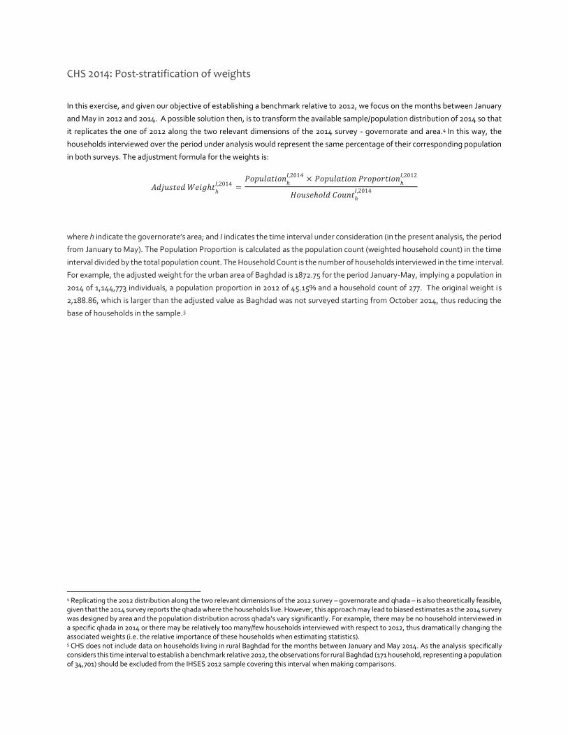
CHS 2014: Post-stratification of weights

In this exercise, and given our objective of establishing a benchmark relative to 2012, we focus on the months between January

and May in 2012 and 2014. A possible solution then, is to transform the available sample/population distribution of 2014 so that

it replicates the one of 2012 along the two relevant dimensions of the 2014 survey - governorate and area.4 In this way, the

households interviewed over the period under analysis would represent the same percentage of their corresponding population

in both surveys. The adjustment formula for the weights is:

𝐴𝑑𝑗𝑢𝑠𝑡𝑒𝑑 𝑊𝑒𝑖𝑔ℎ𝑡ℎ

𝐼,2014 =𝑃𝑜𝑝𝑢𝑙𝑎𝑡𝑖𝑜𝑛

ℎ

𝐼,2014 × 𝑃𝑜𝑝𝑢𝑙𝑎𝑡𝑖𝑜𝑛 𝑃𝑟𝑜𝑝𝑜𝑟𝑡𝑖𝑜𝑛ℎ

𝐼,2012

𝐻𝑜𝑢𝑠𝑒ℎ𝑜𝑙𝑑 𝐶𝑜𝑢𝑛𝑡ℎ

𝐼,2014

where h indicate the governorate’s area; and I indicates the time interval under consideration (in the present analysis, the period

from January to May). The Population Proportion is calculated as the population count (weighted household count) in the time

interval divided by the total population count. The Household Count is the number of households interviewed in the time interval.

For example, the adjusted weight for the urban area of Baghdad is 1872.75 for the period January-May, implying a population in

2014 of 1,144,773 individuals, a population proportion in 2012 of 45.15% and a household count of 277. The original weight is

2,188.86, which is larger than the adjusted value as Baghdad was not surveyed starting from October 2014, thus reducing the

base of households in the sample.5

4 Replicating the 2012 distribution along the two relevant dimensions of the 2012 survey – governorate and qhada – is also theoretically feasible, given that the 2014 survey reports the qhada where the households live. However, this approach may lead to biased estimates as the 2014 survey was designed by area and the population distribution across qhada’s vary significantly. For example, there may be no household interviewed in a specific qhada in 2014 or there may be relatively too many/few households interviewed with respect to 2012, thus dramatically changing the associated weights (i.e. the relative importance of these households when estimating statistics). 5 CHS does not include data on households living in rural Baghdad for the months between January and May 2014. As the analysis specifically considers this time interval to establish a benchmark relative 2012, the observations for rural Baghdad (171 household, representing a population of 34,701) should be excluded from the IHSES 2012 sample covering this interval when making comparisons.

poverty in iraq, 2012 - 2014 - world...

Documents