Potentials and Implications of Dedicated Highway Lanes forAutonomous Vehicles

Jordan Ivanchev1, Alois Knoll2, Daniel Zehe1, Suraj Nair1, and David Eckhoff1

1TUMCREATE, Singapore2Department of Informatics, Technische Universität München, Germany

September 25, 2017

Abstract

The introduction of Autonomous Vehicles (AVs) will have far-reaching effects on road traffic in citiesand on highways.The implementation of Automated Highway Systems (AHS), possibly with a dedicatedlane only for AVs, is believed to be a requirement to maximise the benefit from the advantages of AVs.We study the ramifications of an increasing percentage of AVs on the traffic system with and without theintroduction of a dedicated AV lane on highways. We conduct an analytical evaluation of a simplifiedscenario and a macroscopic simulation of the city of Singapore under user equilibrium conditions with arealistic traffic demand. We present findings regarding average travel time, fuel consumption, throughputand road usage. Instead of only considering the highways, we also focus on the effects on the remainingroad network. Our results show a reduction of average travel time and fuel consumption as a result ofincreasing the portion of AVs in the system. We show that the introduction of an AV lane is not beneficialin terms of average commute time. Examining the effects of the AV population only, however, the AVlane provides a considerable reduction of travel time (≈ 25%) at the price of delaying conventional vehicles(≈ 7%). Furthermore a notable shift of travel demand away from the highways towards major and smallroads is noticed in early stages of AV penetration of the system. Finally, our findings show that after acertain threshold percentage of AVs the differences between AV and no AV lane scenarios become negligible.

1 IntroductionAutonomous vehicles have ceased to be only a vision but are rapidly becoming a reality as cities around the worldsuch as Pittsburgh, San Francisco, and Singapore have begun investigating and testing autonomous mobilityconcepts [1]. The planned introduction of thousands of autonomous taxis, as currently planned in Singapore [1],poses a challenge not only to the in-car systems of the AV, but also to the traffic system itself.

Besides the deployment of more efficient ride sharing systems and the reduction of the total number ofvehicles on the road, AVs can traverse a road faster while using less space. To achieve the maximum benefitin terms of traffic speeds and congestion reduction, however, mixing of AVs and Conventional Vehicles (CVs)should be avoided [2]. One method to achieve this is the introduction of dedicated AV lanes on highways toallow AVs to operate more efficiently due to the absence of unpredictable random behaviour introduced byhumans and the use of communication capabilities, e.g. platoon organization [3].

Blocking certain lanes for CVs, and thereby limiting the overall road capacity for human drivers is certainlya step that can have considerable ramifications, depending on the portion of AVs in the system. While at theearly stages, where only few AVs are on the road, it would constitute an incentive to obtain an AV, it couldalso possibly generate traffic congestion and increase travel times for other vehicles [4]. As the level of AVpenetration in the road transportation system is increased, the total congestion level would likely drop, however,the advantage of using AVs over CVs would gradually be diminished as well.

Lastly, converting highways into AHS could also affect the rest of the road network, as drivers of CVs maythen choose a different route, caused by the changed capacity of the highway, which can lead to a mismatchbetween road network and traffic demand [5].

In this paper, we take a closer look at the benefits and drawbacks of introducing a dedicated AV lane onmajor highways Singapore. Focusing particularly on the effect of varying percentages of AVs in the system, westudy the differences in terms of capacity, travel time, fuel consumption, and impact on other roads comparedto a setting where no dedicated AV lane is assigned. In short, our two main contributions are:

• We present an analytical evaluation of the expected benefit from the introduction of dedicated AV lanes.

1

arX

iv:1

709.

0765

8v1

[cs

.MA

] 2

2 Se

p 20

17

• Using a macroscopic traffic simulation of the city-state of Singapore and based on realistic travel demand,we show the impact of vehicle automation with and without AV lanes.

The remainder of this paper is organized as follows: In Section 2 we discuss related work on AHS. Section 3explains the system model used in this study. In Section 4 we present our analytical evaluation of a syntheticscenario, followed by Section 5 in which results for the entire city of Singapore are presented and discussed.Section 6 concludes our article.

2 Related WorkAHS and their implications have received wide attention from both researchers and industry around the world.Investigations include general AHS policies and concepts [2,6], effects on travel times and capacity [6–13], trafficsafety [6, 8, 13,14], and interactions between conventional human-driven vehicles and autonomous vehicles [15].

Several AHS studies and field trials were conducted as part of the California Partners for Advanced Transitand Highways (PATH) program: Tsao et al. discuss the relationship between lane changing manoeuvres andthe overall throughput of the highway [9]. Their analytical and simulation results indicate a direct trade-offbetween the two. Lateral movement decreases the traffic flow, and higher traffic flow leads to longer lane changetimes. In this work, we ignore decreased throughput caused by lane changing and focus on a best-case city-widebenefits of dedicated AV lanes. Godbole and Lygeros evaluate the increased capacity by the introduction of fullyautomated highways by treating the highway as a single-lane AHS pipe [14]. Similar to the work of Harwoodand Reed [10], they study different platoon sizes and speeds but do not consider separated AV and CV lanes.

AHS pipeline capacity was also studied by Michael et al. [11]. Their results show that longer platoons of AVsare favourable as they increase the capacity of the road due to lower inter-platoon distances. A high mixture ofdifferent vehicle classes, however, leads to a lower capacity. Lastly, the presented analytical model shows thatas highway speed increases, the capacity reaches a saturation point after which the speed decreases again. Thisis inline with the findings presented in this paper when studying the throughput on only the AV lane.

Similar to the work presented in this article, Cohen and Princeton investigated the impact of dedicatedlanes on the road capacity [7]. They find that assigning a dedicated lane can create bottlenecks due to increasedlane changing manoeuvres of departing unauthorized vehicles. When the capacity of the remaining lanes isexceeded, it may even be impossible for allowed vehicles to access the dedicated lane. In our macroscopicstudy, we abstract away from these problems to answer the more general question whether the introduction ofdedicated AV lanes is a feasible approach.

In summary, it appears that while AHS seem to be a well-studied subject, a general evaluation of theintroduction of AV lanes is still missing. Furthermore, automated highways are mostly investigated in anisolated manner (and often also simplified to a 1-lane road) without taking into considering the rest of the roadnetwork. Using the city-state of Singapore as a case study, we show how travel times of both AVs and CVs areaffected and that the introduction of dedicated AV lanes has a considerable effect on the entire road networkby changing the distribution of traffic demand within the transportation system.

3 System ModelThe goal of this study is to evaluate the allocation of one lane on every highway road to be used exclusivelyby autonomous vehicles. We investigate an increasing percentage of AVs in the system under two scenarios:with and without dedicated AV lanes on highways. In the former scenario, all roads that are not highwayswill exhibit normal traffic conditions as there will be a mixture of human drivers and AVs. All lanes on thehighway roads will be accessible to AVs, while CVs will be able to utilize all lanes except one lane, which willbe allocated exclusively for AVs usage.

In the second scenario, all vehicles will share all lanes on all roads.We model the different behaviour of AVs and CVs by means of smaller headway time, that is the time gap

to the vehicle in front. We assume that AVs can afford a much smaller headway than normal vehicles sincetheir reaction time is orders of magnitude smaller than that of humans [16]. A direct consequence of this isthat effectively the capacity of the road is increased, as AVs need less space. The capacity (in cars per hour perlane) can then be calculated as follows:

C =3600

havpav + hcv (1 − pav)(1)

where hav is the headway time for AVs (values may vary between 0.5 and 1 second, depending on levelof comfort [13]), pav is the percentage of AVs on the road segment, hcv is the headway time for conventionalvehicles set to 1.8 seconds. Equation 1 is based on [17], where it was derived from collected data on highwayroads in Japan for varying percentages of vehicles with AHS.

2

Figure 1 illustrates the change of capacity as a function of the AV percentage for different AV headwayvalues. It can be observed that the capacity exponentially increases with the portion of AVs on the road. Thismeans that when there is a small portion of AVs on a road, their impact is only marginal, however, when themajority of vehicles are AVs there is a significant increase of the capacity of the road. The capacity for the sameAV percentage also increases exponentially as the headway time decreases. For the remainder of the paper wewill assume a conservative AV headway of hav = 1s.

0 0.2 0.4 0.6 0.8 1Portion of AVs

2000

4000

6000

8000La

ne C

apac

ity [v

ehic

les/

hour

]Headway=1sHeadway=0.75sHeadway=0.5s

Figure 1: Changes of road capacity as a function of AV percentage and headway time

The primary measure we use to evaluate the impact on traffic caused by the introduction of an AV lane isthe travel time of cars. The travel time T =

∑ni ti of a vehicle is determined by the traverse times of all n

segments (or links) included in its route. The traverse time ti of a segment i can be computed using the Bureauof Public Roads (BPR) function [18]:

ti =livi

(1 + αi

(Fi

Ciwit

)βi)

(2)

where li is length of the road segment, vi is the free flow velocity of the segment, Fi is flow, wi is the number oflanes, t is time duration of the simulated period, Ci is the capacity of road segment i, αi and βi are parametersfrom the BPR function. Free flow velocities v̂ are extracted from historical GPS tracking data [19]. Parametersαi and βi are calibrated for different classes of roads depending on their speed limits using both GPS trackingdata and a travel time distribution of the population for certain periods of the day. For a more detaileddescription of the calibration and validation procedures we refer the reader to [20].

4 Analytical EvaluationIn this section, we will illustrate how to analytically determine the travel times of vehicles on highways in bothcases with and without dedicated AV lanes. We examine a simplistic scenario, where the system consists of asingle road with two lanes. Let the overall percentage of AVs be p and the percentage of AVs on the first andsecond lane respectively be p1 and p2. Let the number of vehicles on the respective lanes be f1 and f2 suchthat:

f1 + f2 = F (3)

where F is the total number of vehicles in the system. Therefore, we know that:

p1f1 + p2f2 = pF (4)

Under the assumption of User Equilibrium (UE) [21] we also know that:

t(f1) = t(f2) (5)

where t(f) represent the travel time on the road for flow f . UE is achieved when given the current trafficsituation, a user would not change their route, i.e. the user is already on the shortest route in terms of traveltime.

3

Substituting t(f) for the BPR function (Equation 2) we get:

t(f) =l

v

(1 + α

(f

C

)β)(6)

Where α and β are parameters of the BPR function, v and l are the free flow velocity, and the length of theroad and C is the capacity of the road. Substituting the expression for capacity from Equation 1 we get for theBPR function:

t(f) =l

v

(1 + α

(f (havpav + hcv (1 − pav))

3600

)β)(7)

Expanding Equation 5 we get:

l

v

(1 + α

(f1 (havp1 + hcv (1 − p1))

3600

)β)=l

v

(1 + α

(f2 (havp2 + hcv (1 − p2))

3600

)β)

Removing common terms, simplifying and using Equations 3 and 4 we get:

f1 (havp1 + hcv (1 − p1)) = (hav (pF − p1f1) + hcv (F − f1 − (pF − p1f1)))

Let’s examine the two scenarios in this simplistic example: In scenario 1 a lane is exclusively reserved forAVs (p1 = 1) and in scenario 2 all cars are allowed to use all lanes and therefore get distributed equally on thetwo lanes (f1 = f2 = F

2 and p1 = p2 = p). For scenario 1 we get:

f1hav = hav (pF − f1) + hcvF (1 − p) (8)

After simplifying we obtain:

f1hav =F

2(havp+ hcv (1 − p)) (9)

Under the assumption of user equilibrium it follows that for scenario 1 the travel time for both lanes is thesame:

t1 =l

v

(1 + α

(f1hav3600

)β)(10)

The travel time for a single vehicle in scenario 2 is:

t2 =l

v

1 + α

F

2(havp+ hcv (1 − p))

3600

β (11)

It can be observed that because of Equation 9 the expression in Equation 10 is equal to the expression inEquation 11. This means that in the simple examined case, regardless whether a dedicated AV lane is introducedor not, the resulting travel time for all commuters is going to be the same after the point where there are enoughAVs to ensure equilibrium can be reached.

The number of vehicles on the first lane in scenario 1 is bounded from above by the total number ofautonomous vehicles: f1 ≤ pF . In the case where f1 computed according to Equation 9 is smaller than pFequilibrium cannot be achieved. It is trivial to demonstrate that the overall travel time under scenario 1 isbigger than the travel time under scenario 2 when f1 ≤ pF . The minimum number of AVs in terms of the AVpercentage pτ (the threshold percentage) in order for the solutions of the two scenarios to coincide is:

pτFhav =F

2(havpτ + hcv (1 − pτ )) (12)

pτ =hcv

hav + hcv(13)

The percentage pτ describes the point where for an additional AV it would be equally attractive to use theAV lane or the normal lane. This is the moment where the AV lane reaches saturation. Before that percentageis reached, the AVs have a shorter commuting time than the CVs, however, the system is performing worse

4

in terms of overall congestion compared to the case without a dedicated AV lane. Equation 13 can be easilyextended for an arbitrary number of lanes in our minimalistic example. Assume we have 1 dedicated AV laneand N normal lanes. Then the percentage of AVs after which the dedicated lane is saturated becomes:

pτ =hcv

Nhav + hcv(14)

Assuming headway times of hcv = 1.8s and hav = 1s, the percentage pτ of AVs on the road for saturationof the AV lane is 64.3%, 47.4%, 37.5%, 31%, 26.5% for respectively 2, 3, 4, 5, 6 lane roads with one allocatedAV lane.

5 City-wide Simulation StudyWe conduct a macroscopic city-wide simulation study of the city-state of Singapore to better understand theeffects to be expected in a complex environment. We take a look at the traffic conditions on the highway, butalso closely investigate the effect dedicated AV lanes have on the rest of the road network.

5.1 MethodologyIn order to evaluate the scenarios of AV introduction in a road transportation system, we make use of an agent-based macroscopic simulation approach. The simulation consists of three steps: 1) Agent generation, 2) routecomputation and 3) travel time estimation.

The underlying road network on which the traffic assignment is performed is modelled by means of a uni-directional graph, where each edge represents a road segment and nodes represent decision points at which aroad may split or merge.

To introduce dedicated AV lanes, we alter the original graph by duplicating start and stop nodes of highwaysegments and creating a new edge to represent the AV lane, while removing one of the normal lanes fromthe original segment. Furthermore, costless connections are added between the start and end nodes and theirrespective copies so that vehicles can change lanes at the start/end of highway road segments.

Every agent is generated with an origin and destination sampled from an OD matrix representing the traveldemand of the system. Realistic traffic volume is modelled by synthesizing a sufficiently large vehicle populationaccording to the available survey data.

The routes of the agents are computed using an incremental user equilibrium approach [21] aiming atrepresenting reality in the sense that every driver is satisfied with their route and would not choose a differentone given the current traffic situation. We assume a driver is satisfied when they are on the shortest route fromorigin to destination in terms of travel time. Routing is performed on the road network graph, where each edgehas an attached weight representing the current traverse time of this road segment. Weights are updated afterevery batch route computation. To disallow conventional vehicles from using the AV lane, the weight of theedges representing these lanes are set to infinity when the route of a CV is computed and set back to theirtraverse time values for AV route computation.

Further assumptions regarding to the macroscopic level of the simulation include:

• Agents want to minimize travel time and all perceive the traffic situation in the same way (there is nonoise in the observations of the traffic states).

• Traffic is spread homogeneously in time during the simulation. In order for the BPR function (Equation2) to give a reasonable estimation of the traffic conditions, the flow F during the simulation time t needsto be spread homogeneously in time. If many vehicles try to enter the road at the same time for example,the traffic congestion generated will likely produce a much higher traverse time for the road than theexpected one. In order to ensure as much as possible that traffic demand stays static throughout thesimulation period, both the period t and the time of day, which is simulated, have to be chosen with care.

• Agents do not reroute while on their trip. In reality drivers may change their trip plan dynamicallyaccording to unexpected events or observed traffic conditions ahead. As our traffic assignment providesinformation to the drivers about expected traffic conditions for the whole network, we assume that suchevents will not occur as drivers are given all the information they need prior to their trip.

5.2 Data and Scenario DescriptionWe examine the city-state of Singapore with a total population of 5.4 million and around 1 million registeredvehicles including taxis, delivery vans and public transportation vehicles. The fact that Singapore is situatedon an island simplifies our scenario as the examined system is relatively closed with only two expressways

5

leading out of the country. There are 3495 km or roads of which 652 km are major arterial roads and 161km are expressways (these are the roads on which we introduce the dedicated AV lane indicated on Figure 5a)spreading over 715 squared km of land area. We have used publicly available data to acquire a unidirectionalgraph of Singapore, that comprises of 240, 000 links and 160, 000 nodes representing the road network of thecity. The number of lanes, speed limit and length of every link is available allowing us to extract informationabout its capacity.

For the purposes of our model we make use of two separate data sets. The first data set consists of GPS tra-jectories of a 20, 000 vehicle fleet for the duration of one month, providing information about recorded velocitieson the road network during different times of the day [19]. The second one is the Household Interview TravelSurvey (HITS) conducted in 2012 in the city of Singapore, which studies the traffic habits of the population.Information about the origin destination pairs, their temporal nature, and commuting time distribution duringrush hour periods is extracted from it.

In order to achieve realistic traffic conditions, we estimated the number of agents based on the SingaporeHITS data. We extracted the ratio of people who actively create traffic on the streets (cab drivers, personalvehicle drivers, lorry drivers) and the total number of people interviewed.

We chose the morning commute hours (7:30am - 8:30am) as the period which seems to be the most stablein terms of traffic volume and estimated the traffic demand consisting of 309, 000 agents.

Similar to the simplistic example the vehicle population is split into two parts: AV and CV. The percentageof AV is varied in order to observe the effects in the initial stages of AV introduction, as well as the possibletraffic situation if all vehicles were autonomous.

In order to have a benchmark for measuring the efficiency of the suggested policy, we also evaluate thescenario where no AV lane is introduced and all vehicles can access all lanes on all roads. The analyticalsolution acquired for the simplistic example in the previous section indicates that the scenario with no AV lanewill produce better or at least the same system performance as the introduction of the AV lane. Our case studywill test our analytical results for a more realistic transportation system environment.

5.3 Effects on Average Travel TimeWe evaluated the change in average commute time based on the percentage of AVs in the system. We comparetwo different settings: with and without a dedicated AV lane. As a baseline we use the average commute timewithout the existence of AVs (and thus no exclusive lanes). This time was found to be approx. 18.5 minutesand can be seen as the status quo.

We simulated both settings with the exact same travel demand, that is, identical origin-destination pairs forall vehicles. We then gradually increased the percentage of AVs in the system. The number of vehicles in thesimulation was invariant; a higher percentage of AVs means that CVs were replaced with autonomous vehicles.

Figure 2 shows our result.

0 0.2 0.4 0.6 0.8 1

Portion of AVs

14

15

16

17

18

19

20

Ave

rage

Tra

vel T

ime

[min

s] AVsCVsOriginal Scenario

(a) Travel times with dedicated AV lane

0 0.2 0.4 0.6 0.8 1

Portion of AVs

14

15

16

17

18

19

20

Ave

rage

Tra

vel T

ime

[min

s] With AV LaneWithout AV LaneOriginal Scenario

(b) Comparison for all vehicles

Figure 2: Average travel time of whole population, AVs and CVs as a function of AV percentage

The black dashed line serves as an illustration of the status quo. It can be observed that when introducinga lane exclusively for AVs and thereby taking away capacity from conventional vehicles (Figure 2a), the traveltime for CVs increases, whereas the low percentage of AVs (driving on almost empty lane) travel considerablyfaster. This could be used as an incentive by policy-makers to increase the share of AVs in the transportationsystem. With an increasing percentage of AVs we observe that travel times for CVs decrease due to the factthat effectively vehicles move away from the common lane to the AV lane, which in turn increases the traveltime on the AV lane. This behaviour can be observed until the AV lane is saturated (somewhere between 40%and 50% AV percentage). From this point on, the choice of lane makes no difference for newly added AVs

6

as they experience equal travel times regardless whether they choose to take the AV lane or the mixed lane.Therefore, the difference between average travel time of AV and CV decreases. Travel time of both AVs and CVsstill decreases with the increase of the percentage of AVs since the capacity of the road network is effectivelyincreased.

The average number of lanes in the Singapore road network is 3.14. If we apply Equation 14 from ouranalytical evaluation, we yield a saturation point of 45.2% AV penetration, which seems to be in agreementwith our simulation results.

We conclude that computing the threshold percentage is useful in terms of AV lane introduction planning.Figure 2b shows the comparison between the average travel times for the entire vehicle population with

and without the introduction of an AV lane. It can be observed that the setting without an AV lane is alwaysperforming better than the AV lane one. After saturation of the AV lane the difference between the two curvesbecomes marginal. This finding is in complete agreement with the results of our analysis in Section 4. Beforesaturation of the AV lane, the capacity of the highway is not fully utilized and that, on average, the smallertravel times of the AVs cannot make up for the introduced delays for the CVs. We conclude that adding an AVlane, while initially being an incentive for early adopters, will noticeably penalize drivers of conventional vehiclesat the early stages of AV introduction. Additional delays will be introduced by lane changing manoeuvres andother microscopic effects not considered in this macroscopic study [7, 9].

5.4 Analysis of Effect of Headway TimeThe headway time of vehicles is a crucial parameter for the computation of the road capacity (see Equation 1)and therefore an important input for the travel time computation using the BPR function (see Equation 2).

Although, AVs can afford to have smaller headways, this might negatively affect the comfort of the passengers,as small distances at high velocities can induce anxiety [13]. To this end, we examine the effect of varying theheadway time (from 0.5s to 1s) for the city-scale simulation scenario with a dedicated AV lane on highways. Itis therefore useful to evaluate the amount of overall travel time decrease as a function of the headway time.

0 0.2 0.4 0.6 0.8 1

Portion of AVs

13

14

15

16

17

18

19

20

Ave

rage

Tra

vel T

ime

[min

s]

Headway=0.5sHeadway=0.75sHeadway=1sOriginal Scenario

Figure 3: Average travel time curves for varying headway time

In Figure 3 we observed that, depending on the headway, the improvement of overall travel time can varybetween 20% and 26%. The difference between the improvement in the case of all AVs seems is bigger betweenheadway 0.5s and 0.75s than between 1s and 0.75s.

This is due to the non-linear nature of the BPR function. As vehicles approach free flow velocities due tothe increased capacity, any further improvement in capacity plays a smaller role and therefore the gains becomeless significant. It must be noted, that this happens only when traffic congestion is such that vehicles travel atfree flow velocities.

If the system was more congested, we would not be able to observe the decrease of travel time improvementfor smaller headway time, since the BPR function will still be in its non-linear part thus providing significantchanges of travel time as the capacity is altered.

5.5 Effects on Fuel ConsumptionWe have demonstrated that the introduction of AVs decreases the overall travel time in the system. The nextquestion we are trying to answer is by how much this saved time reduces fuel consumption (or energy in the

7

case of electric vehicles). We deploy the Elemental fuel consumption model [22] to evaluate the average fuelconsumption of the vehicle population and subgroups.

The effects of introducing an AV lane on fuel consumption are shown in Figure 4

0 0.2 0.4 0.6 0.8 1

Portion of AVs

1

1.05

1.1

1.15

1.2

1.25

1.3

Ave

rage

Fue

l Con

sum

ptio

n [li

tres

]

Whole populationAVsCVsOriginal Scenario

Figure 4: Average fuel consumption of whole population, AVs and regular vehicles as a function of AV percentage

As expected, we observe a positive effect on fuel consumption. To provide an idea of magnitude, the fuelsaved at 20% AVs is about 9.3 tons for the duration of one Singapore morning rush hour and approx. 45 tonswhen every vehicle is autonomous. As for the travel time, the combination of one dedicated lane and a lowpercentage of AVs penalizes CVs.

The introduction of more AVs, however, decreases both the overall travel time and fuel consumption. It canalso be noted that the relative effect of the fuel consumption is smaller than the effect on travel time, whichmeans that fuel consumption is less sensitive with respect to changes in the traffic states for the examinedscenario. Please note that we do not consider fuel or energy saving resulting from platoon organization [12] andother AV related technology but only seek to provide a order of magnitude with our macroscopic evaluation.

5.6 Effects on Road Network Throughput and Traffic DistributionLastly, we examine the traffic distribution on the entire road network to gain a better understanding of thechanges occurring in traffic conditions as a results of the introduction of dedicated AV lanes. To the best ourknowledge, existing literature focuses on the traffic changes on the highways and ramps only, and such a studyhas not been conducted before. Figure 5a shows the Singaporean road network with highways drawn in bold.AV lanes are added only to these highways, the rest of the network remained unchanged.

As a first step, we provide a qualitative measurement by visualizing the impact an introduction of 50% AVshas on the road network (compared to 0% AVs). To this end, we draw roads experiencing higher throughputin blue colours and roads experiencing lower throughput in red colours. We show our results for both settings,i.e., with AV lane (Figure 5b) and without AV lane (Figure 5c).

It can be observed that in both cases the highways exhibit a considerably higher throughput of vehicles, whichis expected since the capacity of the highway is technically increased by the introduction of the autonomousvehicles. Other roads exhibit a slight decrease of throughput, which may be due to the changes in routingthat are triggered by the AVs, which have a strong preference towards the highways. In other words, the AVsare, in a way, attracted to the highways, since they can traverse fast there and the capacity is sufficient. This,however, makes them willing to pass through more congested roads in order to get to the highway, which createsadditional time losses for the regular vehicles. This argument is further strengthened by the fact that the roadsleading to the highways do not exhibit increased throughput, although they exhibit higher demand since morevehicles want to use the highways. This means that the level of congestion on those roads is too high to allowan increase of throughput.

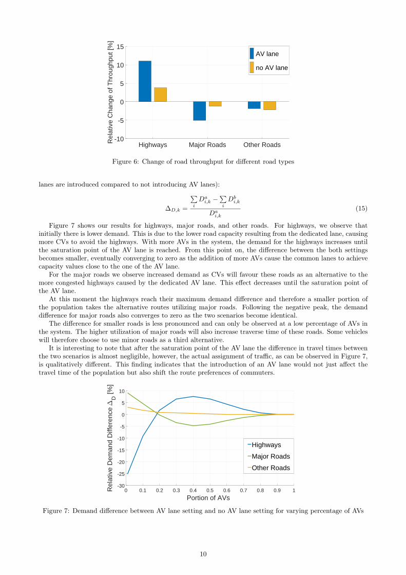
Comparing the throughput changes in the two scenarios, it can be observed that the increase of throughputon the highways for the case with no AV lane is smaller. Therefore, the change of routing triggered by theintroduction of AVs is qualitatively the same but quantitatively different for the two examined scenarios. Thiscan be observed in Fig. 6. The relative increase of throughput for highways is almost three times higher for thededicated AV lane case. Higher level of throughput increase on highways leads to higher level of throughputdecrease on the major roads, which represent alternative routes. As mentioned before, if highways become tooattractive for AVs, there can be negative effects on traffic conditions stemming from overly utilized roads whichlead to the highways. The more balanced distribution of traffic in the no AV lane scenario could be the reason

8

(a) Singapore road network with highways featuring dedicated AVlanes in bold

(b) Change of road throughput at 50% AVs (with AV lane)

(c) Change of road throughput at 50% AVs (without AV lane)

Figure 5: Road throughput change caused by 50% AVs compared to 0% AVs. Colours from the blue gammarepresent higher throughput; colours in the red gamma represent lower throughput

for its slight, however, consistent superiority over the dedicated AV lane case in terms of average travel timeobserved in Figure 2b.

Finally, we investigate the change in demand for different types of roads. We define demand for a road asthe number of vehicles that have this particular road in their route under user equilibrium traffic assignment.Taking a closer look at the difference in travel demand between the scenario with AV lane and the scenariowithout the introduction of AV lane, we measure the relative difference of travel demand between the scenarios.Formally, let the demand for road i for a given AV percentage k be Da

i,k for the AV lane scenario and Dbi,k for

the benchmark scenario without an AV lane. Then, for the different classes of road (highways, major roads,other roads), we compute the difference in demand between the two examined scenarios relative to the AV lanescenario (a negative value therefore means that this particular type of road experiences less demand when AV

9

Highways Major Roads Other Roads-10

-5

0

5

10

15

Rel

ativ

e C

hang

e of

Thr

ough

put [

%]

AV lane

no AV lane

Figure 6: Change of road throughput for different road types

lanes are introduced compared to not introducing AV lanes):

∆D,k =

∑i

Dai,k −

∑i

Dbi,k

Dai,k

(15)

Figure 7 shows our results for highways, major roads, and other roads. For highways, we observe thatinitially there is lower demand. This is due to the lower road capacity resulting from the dedicated lane, causingmore CVs to avoid the highways. With more AVs in the system, the demand for the highways increases untilthe saturation point of the AV lane is reached. From this point on, the difference between the both settingsbecomes smaller, eventually converging to zero as the addition of more AVs cause the common lanes to achievecapacity values close to the one of the AV lane.

For the major roads we observe increased demand as CVs will favour these roads as an alternative to themore congested highways caused by the dedicated AV lane. This effect decreases until the saturation point ofthe AV lane.

At this moment the highways reach their maximum demand difference and therefore a smaller portion ofthe population takes the alternative routes utilizing major roads. Following the negative peak, the demanddifference for major roads also converges to zero as the two scenarios become identical.

The difference for smaller roads is less pronounced and can only be observed at a low percentage of AVs inthe system. The higher utilization of major roads will also increase traverse time of these roads. Some vehicleswill therefore choose to use minor roads as a third alternative.

It is interesting to note that after the saturation point of the AV lane the difference in travel times betweenthe two scenarios is almost negligible, however, the actual assignment of traffic, as can be observed in Figure 7,is qualitatively different. This finding indicates that the introduction of an AV lane would not just affect thetravel time of the population but also shift the route preferences of commuters.

0 0.1 0.2 0.3 0.4 0.5 0.6 0.7 0.8 0.9 1

Portion of AVs

-30

-25

-20

-15

-10

-5

0

5

10

Rel

ativ

e D

eman

d D

iffer

ence

"D

[%]

Highways

Major Roads

Other Roads

Figure 7: Demand difference between AV lane setting and no AV lane setting for varying percentage of AVs

10

6 Conclusion and Future WorkIn this article we demonstrated the effect of assigning one lane on highways exclusively for AVs. We showedthat for lower percentages of AVs, or more precisely, before the dedicated lane is saturated, travel times for AVscan be significantly shorter, while at the same time CVs are delayed due to the reduced capacity of the highway.

Looking at the entire road network, we observe that also non-highways are affected as CVs will effectivelybe drawn away from the highways onto the major roads. This effect is especially pronounced at early stagesof AV adaptation where the AV lane will remain mostly empty. Regardless of an introduction of the AV lane,we confirmed earlier findings that a larger number of AVs will have a positive impact on travel times and fuelconsumption for all vehicles. The macroscopic simulation study confirmed our analytical evaluation where weshowed how to compute the saturation point of the AV lane and illustrated that after this point is reached,the benefits for AV users become negligible. We further compared the scenario with AV lane introduction to abaseline scenario where no changes to traffic regulations are made. The latter scenario outperforms the formerone over the whole range of AV percentages, however, the difference is of considerable amount only before thesaturation point is reached. This finding coincides with our analytical evaluation of the two scenarios.

Future work includes micro (and submicroscopic) studies to further provide insights on the effects of theintroduction of AV lanes. This includes benefits due to smart platooning strategies but also turbulences causedby lateral vehicle movement, e.g., from the on-ramp towards the AV lane. Furthermore, the authors would liketo exchange the UE traffic assignment of the AV group of vehicles with the BISOS algorithm [23], which looksfor a system optimum assignment, in order to check whether the adoption of an AV lane would become morebeneficial in this case.

AcknowledgementsThis work was financially supported by the Singapore National Research Foundation under its Campus forResearch Excellence And Technological Enterprise (CREATE) programme.

References[1] J. Henderson and J. Spencer, “Autonomous Vehicles and Commercial Real Estate,” Cornell Real Estate

Review, vol. 14, no. 1, June 2016.

[2] T. Litman, “Autonomous Vehicle Implementation Predictions – Implications for Transport Planning,”Victoria Transport Policy Institute, Tech. Rep., November 2016.

[3] M. Segata, B. Bloessl, S. Joerer, F. Dressler, and R. Lo Cigno, “Supporting Platooning Maneuvers throughIVC: An Initial Protocol Analysis for the Join Maneuver,” in 11th IEEE/IFIP Conference on WirelessOn demand Network Systems and Services (WONS 2014). Obergurgl, Austria: IEEE, April 2014, pp.130–137.

[4] J. Ivanchev, D. Zehe, S. Nair, and A. Knoll, “Fast identification of critical roads by neural networks usingsystem optimum assignment information,” in Intelligent Transportation Systems (ITSC), 2017 IEEE 20thInternational Conference on. IEEE, 2017.

[5] J. Ivanchev, H. Aydt, and A. Knoll, “Spatial and temporal analysis of mismatch between planned roadinfrastructure and traffic demand in large cities,” in 2015 IEEE 18th International Conference on IntelligentTransportation Systems, Sept 2015, pp. 1463–1470.

[6] A. Kanaris, P. Ioannou, and F.-S. Ho, “Spacing and Capacity Evaluations for Different AHS Concepts,” inAutomated Highway Systems. Springer, June 1997, pp. 125–171.

[7] S. Cohen and J. Princeton, “Impact of a Dedicated Lane on the Capacity and the Level of Service of anUrban Motorway,” Procedia-Social and Behavioral Sciences, vol. 16, pp. 196–206, July 2011.

[8] J. Carbaugh, D. N. Godbole, and R. Sengupta, “Safety and Capacity Analysis of Automated and ManualHighway Systems,” Transportation Research Part C: Emerging Technologies, vol. 6, no. 1, pp. 69–99,February 1998.

[9] H. Tsao, R. Hall, and B. Hongola, “Capacity Of Automated Highway Systems: Effect Of Platooning AndBarriers,” Institute of Transportation Studies, University of California, Berkeley, Tech. Rep. UCB-ITS-PRR-93-26, February 1994.

[10] N. Harwood and N. Reed, “Modelling the impact of platooning on motorway capacity,” in Road TransportInformation and Control Conference 2014 (RTIC 2014). London, UK: IET, October 2014.

11

[11] J. B. Michael, D. N. Godbole, J. Lygeros, and R. Sengupta, “Capacity Analysis of Traffic Flow Over aSingle-Lane Automated Highway System,” Journal of Intelligent Transportation System, vol. 4, no. 1-2,pp. 49–80, 1998.

[12] R. Hall and C. Chin, “Vehicle sorting for platoon formation: Impacts on highway entry and throughput,”Transportation Research Part C: Emerging Technologies, vol. 13, no. 5, pp. 405–420, October 2005.

[13] B. Van Arem, C. J. Van Driel, and R. Visser, “The Impact of Cooperative Adaptive Cruise Control onTraffic-Flow Characteristics,” IEEE Transactions on Intelligent Transportation Systems, vol. 7, no. 4, pp.429–436, December 2006.

[14] D. N. Godbole and J. Lygeros, “Safety and throughput analysis of automated highway systems,” Instituteof Transportation Studies, University of California, Berkeley, Tech. Rep. UCB-ITS-PRR-2000-1, January2000.

[15] K. M. Dresner and P. Stone, “Sharing the Road: Autonomous Vehicles Meet Human Drivers,” in TwentiethInternational Joint Conference on Artificial Intelligence (IJCAI’07), vol. 7, Hyderabad, India, January2007, pp. 1263–1268.

[16] P. A. Ioannou and C.-C. Chien, “Autonomous intelligent cruise control,” IEEE Transactions on Vehiculartechnology, vol. 42, no. 4, pp. 657–672, November 1993.

[17] T. Yokota, S. Ueda, and S. Murata, “Evaluation of ahs effect on mean speed by static method,” in FifthWorld Congress on Intelligent Transport Systems, Seoul, South Korea, October 1998.

[18] S. C. Dafermos and F. T. Sparrow, “The traffic assignment problem for a general network,” Journal ofResearch of the National Bureau of Standards, Series B, vol. 73, no. 2, pp. 91–118, 1969.

[19] M. Sindhwani and Q. K. Xin, “Singapore Traffic Information Platform: Enabling Traffic-Aware Applications& Systems,” in 17th ITS World Congress, Busa, South Korea, October 2010.

[20] J. Ivanchev, S. Litescu, D. Zehe, M. Lees, H. Aydt, and A. Knoll, “Determining the Most Harmful Roadsin Search for System Optimal Routing,” TU Munich, Tech. Rep. TUM-I1632, February 2016.

[21] C. Fisk, “Some developments in equilibrium traffic assignment,” Transportation Research Part B: Method-ological, vol. 14, no. 3, pp. 243–255, September 1980.

[22] W. F. Faris, H. A. Rakha, R. I. Kafafy, M. Idres, and S. Elmoselhy, “Vehicle fuel consumption and emissionmodelling: an in-depth literature review,” International Journal of Vehicle Systems Modelling and Testing,vol. 6, no. 3-4, pp. 318–395, 2011.

[23] J. Ivanchev, D. Zehe, V. Viswanathan, S. Nair, and A. Knoll, “Bisos: Backwards incremental systemoptimum search algorithm for fast socially optimal traffic assignment,” in 2016 IEEE 19th InternationalConference on Intelligent Transportation Systems (ITSC), Nov 2016, pp. 2137–2142.

12