Potential Effects of the Great Recession on the U.S. Labor Market

William T. Dickens Robert K. Triest Department of Economics Research Department Northeastern University and Federal Reserve Bank of Boston The Brookings Institution

Preliminary draft – please do not cite without permission.

Prepared for the Federal Reserve Bank of Boston Conference on the Long Term Effects of the Great Recession, Oct. 18-19, 2011.

The views expressed in this paper are those of the authors, and do not represent the views of the Federal Reserve Bank of Boston or of the Federal Reserve System. Thanks to Jamie Fogel for outstanding assistance with the SIPP data analysis. Thanks also to Tess Forsell, Matthew Jordan, Marie Lekkas, Elizabeth Meyer, Shaun O’Brian, and Irena Tsvetkova for their help in preparing this paper.

  2  

Introduction    

Past recessions in the United States have not left many scars. Wage movements over past

business cycles are hard to detect, labor force participation rates quickly return to trend levels,

and unemployment rates show no long term effects after typically quick recoveries. Other

countries haven’t been as lucky. At least since Blanchard and Summers (1986) it has been noted

that many other OECD countries experience long drops in labor market participation and

persistent high unemployment.

It has been suggested (for example, Ball (1999)) that U.S. exceptionalism in this regard is

due to our experiencing quick recoveries in output after our recessions. Indeed, none of our

postwar recessions have been particularly protracted until now. Will that difference, or any other

aspect of the great recession, cause medium or long-term changes in the operation of the U.S.

labor market?

We focus on a few areas where previous research and recent discussions have suggested

that there may be medium to long-term effects. One area where the Great Recession may have a

substantial impact is on the wage and earnings of workers displaced during the recession.

Workers who have been displaced from long-term jobs may lose the value of job-specific skills,

and need to search anew for an employment situation to which they are well matched. As a

result, such workers may suffer persistent decreases in labor market earnings. Displacement may

also have persistent effects on probabilities of future job separations and on the aggregate job

finding rate. Workers who regain employment after displacement from long-term jobs may be at

higher risk of termination in their new jobs than they were in their former long-term jobs.

Workers displaced from long-term jobs may also have relatively low rates of job finding after

  3  

displacement due to the greater specificity of their human capital. The potential for increased

labor marker churning and relatively slow matching of displaced workers with job opportunities

might contribute to an outward shift of the Beveridge Curve and an increase in the NAIRU. We

evaluate the evidence for this, and examine the degree to which the apparent outward shift of the

Beveridge Curve may reflect structural issues that will persist over a reasonably long horizon.

Related  Previous  Research    

A large increase in the fraction of the unemployed who are experiencing very long spells

of unemployment has prompted concern that the pool of unemployed job searchers may, on

average, be more difficult to match to job openings than has been true at the end of previous

recessions. Nearly all studies of the rate of new job finding show rates falling as the duration of

unemployment increases.1 Two processes could cause this finding. It could be that extended

unemployment makes it difficult for people to find jobs or it could be that those who have

trouble finding jobs are disproportionately represented among the long term unemployed. A

number of studies have attempted to determine the relative importance of these two explanations

for the downward trend in new job finding rates for the long-term unemployed. Most studies,

using a number of different methods to control for individual differences, still find a substantial

downward trend in new job finding rates (Lynch 1985, Arulampalam 2000, Imbens and Lynch

2006). However, all studies rely on restrictive assumptions about the distribution of individual

differences, leaving the findings suspect. Perhaps more important, the rate of job finding at all

durations of unemployment increases considerably when labor demand is stronger (Imbens and

                                                                                                                         1  An  exception  is  that  studies  often  show  an  increase  in  the  rate  of  exit  from  unemployment  around  the  time  that  unemployment  benefits  expire.  

  4  

Lynch 2006) and it could be that such increases cancel out the effects of longer average durations

of unemployment.

A related literature examines the effect of unemployment spells on future income and the

probability of future employment. Again there is the problem of separating out individual

differences from causal effects. Most typically this is done by comparing people’s experience

before and after a spell of unemployment. These studies often find that spells of unemployment

are followed by a medium to long-term reduction in the wages (Addison 1989, Arulampalam

2001, Corcoran 1982, Farber 2005, Gregg & Tominey 2005, Gregory & Jukes 2001, Jacobson et

al. 1983, Kletzer 1991, Kletzer & Fairlie 2003, Podgursky & Swaim 1987). In a recent paper

using U.S. Social Security records, von Wachter, Song and Manchester (2009) find that workers

who were displaced from stable jobs during the 1982 recession suffered earnings losses of

approximately 20% even after 15 to 20 years. Davis and von Wachter (2011) show that earnings

losses attributable to displacement are roughly twice as large for workers who lose jobs in a

recession compared to those who lose their jobs during an economic expansion. Farber (2011)

documents that the Great Recession has been accompanied by substantial earnings reductions of

job losers, although he notes that it is not yet clear how prolonged the effects will be.

Research suggests that the earnings of young workers are particularly vulnerable to the

effects of recessions. Oreopoulos, von Wachter and Heisz (2006) find that graduating from

college during a recession results in earnings declines lasting ten years. However, von Wachter

and Bender (2006) show that young German workers who leave apprenticeship programs during

a recession generally suffer less persistent earnings losses.

  5  

The future employment and earnings of older workers appears to be sensitive to

economic conditions and job displacement. Von Wachter (2007) finds that both job

displacement and economic conditions affect the earnings and employment of older men. Sass

and Webb (2010) show that job loss in one’s early 50 is associated with subsequent further job

loss and spells of unemployment. Johnson and Mommaerts (2011) document that although job

tenure reduces the probability of job loss, age alone offers no protection. Older workers have

slower rates of reemployment than do younger workers, and suffer much larger reductions in

earnings upon reemployment. Bosworth and Burtless (2010) note that while decreased labor

demand works toward reduced employment of older workers during a downturn, falling assets

prices may lead to increased labor supply through a wealth effect. They find that high

unemployment is associated with increased claiming rates for Social Security benefits. Although

they also find that low asset returns work in the opposite direction, the magnitude of this wealth

effect is vey small.

A few studies suggest that long spells of unemployment result in a lower probability of

being employed in the future for broader groups of workers (Arulampalam 2000, Lynch 1985,

Ruhm 1991), but except for Ruhm these were done with British data. Other studies of U.S. data

conclude that there is no long-term scaring effect of unemployment (Corcoran and Hill 1985,

Ellwood 1982, Genda et al. 2010, Heckman & Borjas 1980).

Evidence  from  the  Great  Recession    

With the unemployment rate still hovering near 9%, it is too soon to fully assess the long-

term effects of the Great Recession on labor markets. Recent data, however, can allow us to

gauge the extent to which the Great Recession differed from the period that preceded it. This can

  6  

be helpful in extrapolating the results of research studies based on earlier data to predict how the

Great Recession will affect labor markets as the recovery continues.

The data that we use in this exercise comes from the first seven waves of the 2004 and

2008 panels of the Survey of Income and Program Participation (SIPP). The SIPP is a large

scale sample survey, where households are interviewed every 4 months, and a new panel of

sample members is fielded every few years. In each wave (sample interviews) of the SIPP,

household respondents answer questions that refer to the preceding 4 calendar months, with the

particular calendar months covered in a wave dependent on the rotation group that the household

is assigned to. The first wave of the 2004 panel covers October 2003 through April 2004, and

the seventh wave covers October 2005 through April 2006. The first wave of the 2008 panel

covers May through November 2008, and the seventh wave covers the same months of 2010.

The first seven waves of the 2004 panel provides data for a 28 month stretch that ends well

before the onset of the recession, with wave 7 data referring to months exactly 2 years after those

covered in wave 1. The first seven waves of the 2008 panel provide similar data for a period of

time that starts in the midst of the recession.

A key advantage of the SIPP is that in wave1, sample members are asked when they had

started their current jobs, allowing researchers to distinguish between long-term and short-term

jobs. The SIPP also records the dates at which sample members start or end jobs when

employment transitions occur over the course of the panel.

Job  Transitions    

  7  

Table 1 compares the experiences of workers who were employed in wave 1 of each of

the two panels.2 Corroborating patterns found in other data, a much higher proportion of

workers observed at the start of the 2008 panel left their job involuntarily (through layoff or

termination) than did workers observed at the start of the 2004 panel. The 2008 panel members

were less likely to leave their wave 1 jobs voluntarily (quits) than were the 2004 panel members;

they were also less likely to stay at their initial jobs over the first seven waves of the panel than

were the 2004 panel members.

The composition of the job losers is important for assessing the long-term effects of job

displacement. If a worker leaves a long-term job, there may be a substantial loss of job-specific

human capital. In contrast, a worker who has been on the job a relatively short time has had little

opportunity to build up capital specific to that job. Workers who have substantial tenure on their

jobs are also likely to be in a situation where both the employee and the employer view the

worker to be well matched to the job. If this were not the case, either party would have

terminated the employment relationship before substantial time on the job had accumulated.

Long-term workers who are displaced from jobs lose that “match capital,” and must again search

for an employment situation that is a good match.

We investigate the composition of job losers in a multinomial logit analysis of job

transitions, the results of which are reported in Table 2. All workers who were employed in

wave 1 are included in the analysis. Workers are classified in terms of how and whether they left

their wave 1 jobs by the end of the wave 7 reference period: workers may have stayed in their

initial job, left that job involuntarily, or left that job voluntarily. We treat staying at the initial

job as the base case, and report the multinomial logit results for the probability of involuntary or

                                                                                                                         2  Workers  holding  more  than  one  job  in  wave  1  were  excluded  from  these  calculations.  

  8  

voluntary transitions relative to staying at the initial job. The analysis is purely descriptive, and

is not intended to capture the parameters of an underlying structural model of employment

transitions. The reported multinomial logit coefficients have been transformed into relative risk

ratios: each coefficient indicates how a unit increase in the conditioning variable affects the

probability of the given outcome (voluntary or involuntary transition) relative to the base case

(staying in the job). A value greater than one indicates increased risk of the outcome relative to

the base case, and a value less than one indicates decreased risk; the reported significance levels

are for rejection of the null hypothesis that the relative risk ratio is equal to one.

The coefficients on the conditioning variables are generally of the expected signs and

magnitudes. Coefficients on dummy variables for job tenure indicate that the probability of

either voluntary or involuntary transition from the job decreases sharply with time for the first

few years of employment. In contrast, the probability of an involuntary transition varies

relatively little with age. Young (less than 25 years old) and old (at least 59 years old) workers

are at significantly higher risk than those in the intermediate groups, but the magnitudes of the

effects are much smaller than those for job tenure. The age effects are larger for voluntary

transitions than they are for involuntary transitions, most likely due to young workers leaving

jobs for schooling, or changing jobs, and older workers leaving jobs for retirement. The

probability of an involuntary job transition decreases sharply with educational attainment; this is

also true for voluntary transitions, but to a lesser extent.

The effect of the Great Recession is measured by an indicator variable for membership in

the 2008 panel (the omitted group is the 2004 panel). The 2008 panel indicator enters the

specification as both a main effect and interacted with the job tenure indicators. The main 2008

panel effect is large for involuntary transitions, although small and statistically insignificant for

  9  

voluntary transitions. The interactions with job tenure are statistically indistinguishable from

one, with the exception of very short tenure workers (less than one year) in the case of

involuntary separations. Experiments with interacting the 2008 panel indicator with other

conditioning variables generally yielded coefficients insignificantly different from one.

An interpretation of the results is that the Great Recession greatly increased the

probability of involuntary job transitions across the board, but did not change the relative

transition probabilities of different types of workers. Young, less educated, and short-tenure

workers were at greater risk of displacement both before and during the recession. Very low

tenure workers were at less of a relative disadvantage during the recession than before the

recession, but this may reflect employers who adopt a last hired-first fired policy needing to

reach further into the tenure distribution when layoffs increase.

Although the relative risks of displacement were not greatly affected by the Great

Recession, this does not imply that the overall increased risk of displacement will not have long-

term consequences. Although long-tenure workers were not disproportionately displaced during

the recession, they were still at increased risk relative to the pre-recession period. To the extent

that displacement of long-tenure workers results in long-term consequences for these workers,

the Great Recession will have a long-term impact through the increase in the number of long-

tenure job matches that were destroyed.

Earnings  Changes    

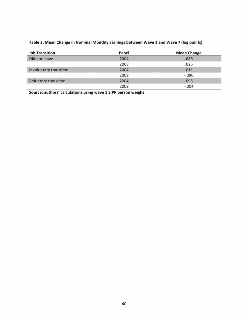
Table 3 displays the mean change in nominal log monthly labor earnings between wave 1

and wave 7 for members of the 2004 and 2008 panels who held jobs in both of these waves,

  10  

shown separately for those who stayed in their wave 1 job, those who voluntarily left their wave

1 job, and those who involuntarily lost their wave 1 job. In interpreting this table, it is important

to remember that the monthly earnings changes can only be calculated for those job changers

who have found new jobs by wave 7. Mean earnings growth was lower in the 2008 panel than in

the pre-recession panel for all three groups. Those who made involuntary transitions fared the

worst both before and during the recession. Nominal monthly earnings increased about 1 percent

for the involuntary job changers over the first 7 waves of the 2004 panel, but fell about 9 percent

in the 2008 panel. Voluntary job changers had the largest monthly earnings increase in the pre-

recession panel, but were second to the job stayers in the 2008 panel. It is evident that job

separations during the recession are having an impact on the monthly earnings of those workers

who are observed in new jobs in wave 7, although it is not clear how long lasting the effect will

be.

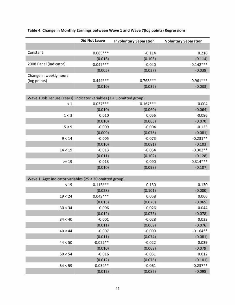
Table 4 shows results from regressions of the change in log monthly earnings between

wave 1 and wave 7 on the change in log weekly hours between waves 1 and 7, worker

characteristics and an indicator for the 2008 panel. The regressions were estimated separately

for job stayers, those making involuntary transitions, and those making voluntary transitions.

The estimated values of the constant and 2008 panel coefficient are essentially providing the

same information as that shown in Table 3, but conditional on changes in weekly hours and

worker characteristics. The regression estimates are not adjusted to account for nonrandom

selection of separated workers into reemployment.

Very few of the worker characteristic coefficients are statistically significantly

discernable from 0. This is somewhat surprising, since one would expect workers with long

tenure in their wave 1 jobs to have experienced a greater loss of earnings than did workers

  11  

displaced from shorter-term jobs. Experiments with interacting worker characteristics with the

2008 panel indicator generally also yielded insignificant coefficients.

The estimated coefficient on the dummy variable for the 2008 panel is negative for all

three groups, but largest in magnitude for workers making involuntary job changes. This is

consistent with the dearth of job openings relative to the number of unemployed during the 2008

panel period, and helps to explain why quit rates fell so much during the recession.

Reemployment  of  Separated  Workers  

In addition to having an influence on the labor earnings of separated workers who regain

employment, the Great Recession may also have affected labor earnings through influencing the

reemployment probabilities of workers leaving jobs. Table 5 shows the estimated coefficients

from multinomial logit analysis of the labor force transitions of workers who leave their wave 1

jobs. The transitions are defined in terms of the wave 7 labor force status (employed,

unemployed, or not in the labor force). The specification was estimated separately for those who

left their wave 1 jobs voluntarily and involuntarily. Reemployment is classified as the base case,

and the coefficients have been transformed into relative risk ratios (with statistical significance

again measured against the null hypothesis that the relative risk ratios equal 1).

Not surprisingly, the results indicate that the probability of unemployment (relative to

reemployment) is much greater in the 2008 panel period than in the 2004 panel; this is true both

for those losing their job involuntarily as well as for those leaving voluntarily. There is not a

statistically significant difference between the two panels in the estimated probability of being

out of the labor force (relative to reemployment).

  12  

Relatively few of the estimated worker characteristic coefficients are statistically

significant. In particular, the job tenure coefficients do not have a statistically significant effect

on the probability of remaining unemployed as of wave 7. This is surprising, since one might

expect the greater specificity of the human capital of long-term employees to make finding a new

job match more difficult. However, it may also be the case that having had a long-term job

signals to potential employers that a job applicant is a reliable employee, possibly resulting in an

increased chance of a job offer.

Conditional on previous job tenure, older workers are significantly more likely than

young workers to remain unemployed. Although the human capital specificity associated with

losing a long-term job does not appear to be an impediment to job matching, age does appear to

be an impediment. Older workers are not only significantly more likely than younger workers to

be unemployed rather than employed, but are also significantly more likely than middle aged

workers to drop out of the labor force after both voluntary and involuntary job separations. The

voluntary separations that lead to being out of the labor force likely reflects planned retirement,

but involuntary separations that lead to being out of the labor force are probably best interpreted

as the unplanned retirements of discouraged workers.

Matching  Efficiency  and  the  Beveridge  Curve    

Although the micro-based evidence on the effects of recessions on separation and job

finding rates is not conclusive, aggregate data suggests that the Beveridge Curve may have

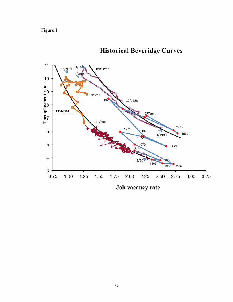
shifted out. Figure 1 shows monthly data for the rate of unemployment and a measure of the

vacancy rate constructed from the Conference Board’s help-wanted index for the period 1980-

1983 and annual average data for those same measures from 1965-1980. The unemployment rate

  13  

and the vacancy rate from the Job Openings and Labor Turnover Survey (JOLTS) for the period

2001-2010/7 is also presented where the JOLTS vacancy rate has been adjusted to be compatible

with the vacancy rate from the help-wanted index.3 Beveridge curves for the 1980-1987 and the

1954-69/2001-09 periods are also drawn. In models of frictional (Blanchard and Diamond 1989,

1991) or mismatch unemployment (Shimer 2005) the Beveridge curve is derived as the locus

where the number of jobs being filled is equal to the number of new unemployed and the number

of new jobs becoming available. On this curve both the unemployment and vacancy rates remain

constant so long as the rate of new job creation and the inflow rate of new unemployed stay

constant. The position of the Beveridge curve is often interpreted as a measure of the efficiency

of worker-job matching. The further the curve is from the origin the more unemployed there are

with the same number of available jobs. The Beveridge curve relation fits remarkably well for

long periods of time. In each of the periods for which the curves are drawn, monthly data on

vacancies and unemployment remained remarkably close to these curves.

Starting a little more than two years ago the vacancy rate began to rise while the

unemployment rate remained mostly unchanged.4 The last time there was a sustained increase in

the vacancy rate, at similar levels of unemployment was during the 1970s. That rise coincided

with a period during which it is widely believed that the NAIRU increased. Similarly, during the

late 1980s and 1990s the level of vacancies that coexisted with a particular level of

unemployment fell and this coincided with a period during which most estimates suggest that the

NAIRU fell (Gordon 1987, Staiger et al. 1997).

                                                                                                                         3  See  Dickens  (2009)  for  an  explanation  of  the  method.  4  In  April  there  was  a  large  increase  in  the  vacancy  rate  that  should  probably  be  ignored  as  it  was  mainly  due  to  government  hiring  for  the  Census.  But,  even  ignoring  that  month,  there  is  still  a  noticeable  increase  in  the  vacancy  rate  over  the  last  year.  

  14  

Dickens (2009) developed and estimated a model of the Beveridge curve and the Phillips

curve that links movement in the Beveridge curve and the position of the long-run Phillips curve

or NAIRU. The results from estimating the model suggest that all shifts in the NAIRU in the

U.S. result from changes in the efficiency of worker-job matching as reflected in movements of

the Beveridge curve. Using this model we can determine the implications of the recent increases

in the vacancy rate for the NAIRU.

Figure 2 presents quarterly estimates of the NAIRU from the model going back to 1960.

It suggests that since 2009 there has been a notable increase in the NAIRU from 5% to just under

6%. Similarly, when we estimate a model allowing for downward nominal wage rigidity to affect

the inflation-unemployment trade-off as in Akerlof et al. (1996), we find that the lowest

sustainable rate of unemployment rises from 3.9% to just over 5%. There is some variation

when we estimate different specifications of these models but all suggest that it would be

possible to lower unemployment by at least 3 percentage points without risking substantial

inflation.

While the model interprets the increase in vacancies as indicating an outward shift in the

Beveridge curve, there are several reasons to question whether the Beveridge curve really has

shifted out. First, the high levels of unemployment we are now experiencing have only been

experienced once before in the period under study and at that time the monthly values strayed

away from the curve that prevailed before and after the recession. In that case the departure

suggested an inward shift in the Beveridge curve. But, as time passes this seems less and less

likely. The departure of the observed vacancy and unemployment rates from the neighborhood of

the Beveridge curve in the 1982 recession lasted only about a year while it has been over 2 years

since vacancies began increasing in the current recession with no reduction in unemployment.

  15  

With adjustments to make the JOLTS vacancy rate equivalent to the one derived from the help-

wanted index, the vacancy rate has recently been below that experienced at any other time in the

sample period. If there is some minimum level of vacancies that are always present (seasonal

jobs that must be filled, firms looking for highly qualified labor at significantly below market

wages) then the Beveridge curve will not have the same shape in the vicinity of that minimum. In

figure 1 it could bend in to the right as the level of vacancies approached that minimum. That

would reduce the extent to which the current level of vacancies departs from the 2001-2009

Beveridge curve.

Note also that the Beveridge curve is the locus where the unemployment rate and the

vacancy rate will settle given a constant rate of new job creation and entry of new unemployed to

the labor market. During a recession these rates aren’t constant. When the rate of new job

creation falls, initially the vacancy rate declines faster than the unemployment rate increases.

During an expansion, the opposite happens as new job creation causes the vacancy rate to rise

before the unemployment rate begins to fall. These tendencies are exacerbated as frustrated

workers leave the labor market when jobs are hard to find (causing the increase in the

unemployment rate to lag the decline in vacancies) and enter the labor market as they become

easier to find (causing the decline in the unemployment rate to again lag the change in

vacancies). This leads to a clockwise movement around the Beveridge curve as it is depicted in

figure 1. This is barely apparent in the 1980 and 2001 recessions, but is pronounced in the 1982

recession – the only other time in the sample that unemployment reached current levels.5

                                                                                                                         5  Tasci  and  Lindner  (2010)  have  also  pointed  out  the  tendency  for  the  unemployment-­‐rate-­‐vacancy-­‐rate  points  to  circle  the  Beveridge  curve.  They  present  three  previous  examples,  1975,  1982  and  2001.  As  shown  in  figure  1  the  cycle  in  2001  was  quite  muted.  The  cycle  in  1975  took  place  while  the  Beveridge  curve  was  moving  out.  Their  use  of  quarterly  rather  than  monthly  data  makes  the  2009-­‐2010  move  look  muted  relative  to  the  comparison  periods.  

  16  

It is possible that the failure of unemployment to fall in response to the increase in

vacancies during the last two years is due to the slow response of the unemployment rate to an

increase in the available jobs. But, a direct comparison to what happened in 1982-83 makes this

doubtful. It only took two months after the vacancy rate began to increase before the

unemployment rate began to decline fairly quickly. It has been over two years since the vacancy

rate began to increase in the current recession and the unemployment rate has hardly declined at

all. This seems like too long a lag to be explained by labor market dynamics. We therefore turn

to potential explanations for deterioration in the efficiency of labor market matching.

The research reviewed above on the effects of the duration of unemployment spells on

job finding rates offers some support for the hysteresis in unemployment hypothesis. More

direct evidence on Ball’s hypothesis comes from a study by Laudes (2005). He estimates Phillips

curves for a sample of OECD countries separating out the effect of the rate of unemployment for

those out of work for more than a year and those out of work for less than a year. He finds that

only those out of work for less than a year put downward pressure on prices while those

unemployed for more than a year apparently have no effect on wages.

We have been able to replicate that result nearly exactly in an updated data set that we

have collected. However, the result is not robust to small changes in the specification. In

particular, when the unemployment rate is broken down to as fine a set of categories for duration

as possible, only the category for unemployment of duration 6-12 months puts statistically

significant downward pressure on wages. Further, any set of categories that contains the category

6-12 months will be found to put significant downward pressure on wages while no set of

categories that does not contain it is ever statistically significant or has a large negative

coefficient. This holds true even if countries whose unemployment benefits normally expire after

  17  

6 months are removed from the sample. These results make no sense for the U.S. economy, and

little sense for the rest of the world. A possible explanation for them is that the 6-12 months

category is the one that is most highly correlated with the overall unemployment rate (>.9).

Overall, there is not much evidence to support the hypothesis that extended periods with

high rates of long-term unemployment will lead to an increase in the NAIRU in the U.S., but this

is not to say that there is strong evidence against the hypothesis either. Given that, we turn to the

evidence for other possible explanations for the worsening of labor market efficiency.

Other  Potential  Explanations  for  an  Outward  Shift  in  the  Beveridge  Curve    

There have been three other explanations for a reduction in labor market efficiency that

have been circulating following the rise in the vacancy rate. In response to the increasing

numbers of long-term unemployed, the Federal Government has extended the duration of

unemployment benefits several times. There is considerable evidence that increases in the

duration of unemployment benefits increase unemployment durations and unemployment rates.

In addition, mismatch between the skills of the unemployed and those demanded by employers

has been offered as an explanation. Finally, it has been suggested that a mismatch between the

location of available jobs and unemployed workers might help explain the worsening efficiency

of labor market matching. That problem might be exacerbated by difficulties in the housing and

mortgage markets.

Extended  Unemployment  Benefits    

Several studies have looked at the role unemployment benefits may be playing in

increasing the unemployment rate by extending the time the unemployed are willing to search for

  18  

jobs. Several of these studies use previous estimates of the effects of benefit duration on

unemployment duration to compute the effects of current policy on unemployment (Aaronson et

al. 2010, Elsby et al.). Such studies produce a range of estimates from .4 to 1.8 percentage points.

A problem with these studies is that the estimates of the impact of extended benefits where made

when the unemployment rate was much lower and jobs were easier to find. It is possible that

such estimates overstate the impact in the current recession. Valletta and Kung (2010) take a

different approach to estimating the impact of extended benefits. They compare the

unemployment durations of those who are eligible for unemployment benefits and those who

aren’t as the duration of benefits is extended. They conclude that extended benefits are

increasing the unemployment rate by about .8 percentage points. Valletta and Kung’s estimate of

the impact of extended benefits is very close to our estimate of the increase in the natural rate

and is slightly below the mid range of previous estimates. However, Rothstein (2011) analyses

how extended benefits affect the probability of leaving unemployment, and estimates that the

benefit extensions raised the unemployment rate by only 0.2 to 0.6 percentage points. Thus, it

seems likely that a substantial part of our estimate of the increase in the NAIRU is due to

extended unemployment benefits, but there is uncertainty regarding the precise magnitude. An

important implication of the effect of extended benefits on the increase in the NAIRU is that the

portion of the increase due to extended benefits could be expected to go away as the benefits are

withdrawn as the economy improves.

Skills  Mismatch    

It seems likely that the U.S. will undergo some structural transformation. The housing

boom probably brought more workers into the construction field than can be sustained in the

long-run. The financial sector may contract relative to its pre-recession size as well. To the

  19  

extent that it takes a long time for workers to move from one type of employment to another,

structural shifts could cause extended increases in the equilibrium level of unemployment (Lilien

1982). The 2001 recession seems to have involved a fair amount of structural reallocation

(Groshen and Potter 2003) and this may explain why it took a longer time than usual to bring the

unemployment rate down during the recovery. To what degree is structural mismatch present in

our economy today and has the degree of mismatch increased with the worsening efficiency of

the labor market?

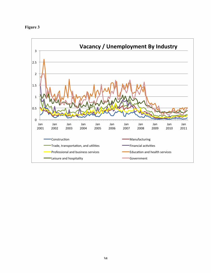
Figure 3 presents the ratio of vacancies to unemployment in several different industries.

While it is possible to discern the increase in vacancies over recent months in some industries,

the ratio remains substantially depressed in all industries. What we do not see is any industries

with high vacancy-unemployment ratios. It is thus hard to make a case for structural mismatch

being a major problem today.

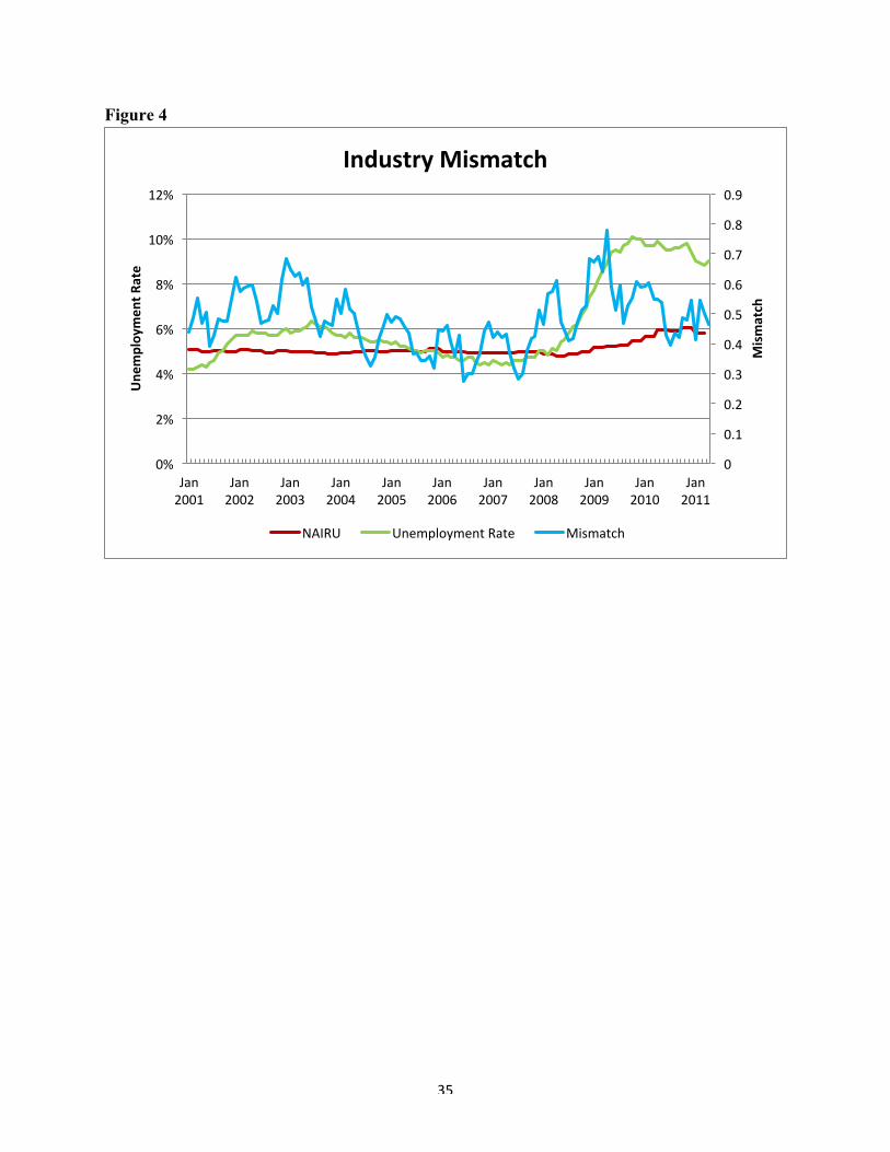
An index of the extent of mismatch between unemployed workers and available jobs can

be constructed by subtracting the fraction of unemployed in each industry from the fraction of

vacancies in each industry and taking its absolute value. This can be thought of as the fraction of

workers who would have to move in order for the fraction of workers unemployed in each

industry to equal the fraction of all vacancies in that industry.6 Figure 4 shows this measure, our

estimate of the NAIRU, and the actual unemployment rate from 2001 to date. While the measure

of mismatch rose considerably during the early phase of the recent recession, it has dropped off

considerably since then and has returned now to levels that prevailed during the mid 2000s when

unemployment was much lower and our estimate of the NAIRU was constant at 5%. The rise

                                                                                                                         6  If  the  matching  function  exhibits  constant  returns  to  scale  and  the  efficiency  of  matching  is  the  same  in  all  cells,  an  allocation  of  the  unemployed  that  equates  the  fraction  of  vacancies  and  unemployed  in  each  cell  will  maximize  the  match  rate  and  minimize  the  unemployment  rate.  

  20  

during the early part of the most recent recession need not reflect a temporary rise in structural

unemployment. Abraham and Katz (1986) showed that business cycles affect different industries

during different phases. This can produce the appearance of structural mismatch which dissipates

as the effects of the recession become widespread.

Although the JOLTS does not contain information on the occupation vacancies are for,

the Conference Board’s Help Wanted Online data do. Researchers at the New York Federal

Reserve (Sahin et al. 2011) have used that data to construct the same sort of mismatch index used

here. They find that there has been an increase in the mismatch between workers and jobs, but

the pattern is similar to that apparent in figure 4 with a rise beginning in late 2006 and a decline

starting in 2009. The timing of these changes suggest that they have nothing to do with the

outward shift in the Beveridge curve. Note that it would be entirely possible for mismatch to

increase and for it to have no impact on structural unemployment if reallocation of workers

between occupations was easy at the margin.

Geographic  Mismatch    

A similar analysis can be conducted for the extent of geographic mismatch, but the

JOLTS data on vacancies are only available at a very high level of aggregation – the four large

Census regions: Northeast, South, Midwest, and West. Figure 5 presents a graph of the mismatch

index by region from 2001 to date along with the NAIRU estimate and the actual unemployment

rate. Not only is there no apparent relationship between the degree of mismatch and our estimate

of the NAIRU, but the fraction of workers who would have to relocate to equalize the fraction of

unemployed and job vacancies in each region has declined. Using the Conference Board’s Help

  21  

Wanted On-line data Sahin et al. (2001) perform a similar exercise at a finer level of

disaggregation and reach the same conclusion.

There is some reason to suspect that a combination of geographic mismatch and problems

in the housing market could be responsible for the reduced level of matching efficiency in the

labor market. In a series of papers Andrew Oswald (1996,1997) has suggested that the level of

the NAIRU in a country is closely linked to the fraction of housing that is owner occupied.7

Oswald argues that high rates of owner occupancy make it difficult for the unemployed to move

when jobs become available elsewhere. In the past, the U.S. has been a huge outlier in this

analysis, having both a high rate of owner occupancy and a low NAIRU. Oswald has explained

this by pointing to the greater ease of transacting sales of housing in the U.S. and the efficiency

of the U.S. mortgage market. However, with a large fraction of the U.S. housing stock

underwater, and the recent tightening of credit standards for mortgages, it is possible that our

high rates of owner occupancy are now making the reallocation of labor substantially more

difficult.

There have been many studies of the effects of “housing lock” on labor market mobility.8

Most studies performed before the recent recession found evidence that distress in housing

markets reduced labor mobility. However, more recent studies generally find little evidence that

long distance moves have been retarded.9 10 An exception to this is the work by Batini et al

                                                                                                                         7  See  Havet  and  Penot  2010  for  a  skeptical  view  of  the  relationship  that  Oswald  points  to.  8  Chan  (2001),  Ferreira  et  al.  (2010),  Henley  (1998),  Schulhofer-­‐Wohl  (2011),  Quigley  (1987  and  2002).  Though  see  Shulhofer-­‐Wohl  (2011)  for  a  different  view.      9  Short  distance  moves  are  defined  as  within  county  and  a  reduction  there  would  be  unlikely  to  affect  job  matching.  10  For  example  see  Donovan  and  Schnure  (2011),  Barnichon  and  Figura  (2011),  and  Molly  and  Smith  (2010).    Modestino  and  Dennett  (2011)  provide  a  survey  of  the  recent  literature,  and  present  evidence  supportive  of  negative  housing  equity  reducing  migration  of  homeowners.    

  22  

(2011) that argues for a substantial role for skills mismatch in combination with a depressed

housing market in increasing unemployment, but the paper has a number of serious flaws. The

conclusions are drawn from a regression of unemployment on skill mismatch, housing market

distress, and an interaction of the two. The first problem is that the index of skill mismatch

compares the level of education of the unemployed not to the demands of available jobs but to

that of the average employed person. Since unemployment rates tend to rise most for the least

skilled during recessions this would induce a positive correlation between mismatch and

unemployment. Second, the correlation between housing market distress and unemployment

could be spurious since both could be due to adverse economic conditions in the state. The

authors recognize this and attempt to ameliorate the problem using the share of subprime

mortgages among all mortgages in the state as an instrument, but this is as likely to be correlated

with economic distress as is the state of the housing market as families with poor employment

prospects may be forced into taking sub-prime loans.

While there is little evidence that housing lock is currently causing structural

unemployment, that could be because there are not enough available jobs to make moving

worthwhile. However, if the housing market remains distressed as the economy picks up, it is

possible that housing market problems could cause problems in the future.

Conclusion    

The Great Recession appears to be exerting an influence on the U.S. labor market that

will likely persist even after economic output has recovered.

  23  

One channel through which job displacement associated with the Great Recession will

likely have a long-term impact is in probabilities of future job separations. Although the relative

risk of job loss did not increase for long-term employees during the recession, their rate of job

loss went up along with those of other groups. And once reemployed, they will be at higher risk

of future job loss because they will have lost the protection afforded by job tenure. One caveat

to this conclusion is that it depends on job tenure being a characteristic of the worker-firm job

match, and not just a factor correlated with worker characteristics that are desirable and

observable to employers, but unobservable to researchers.

Although involuntary job loss is associated with decreased earnings in the short term, it is

puzzling that this effect does not appear to be especially strong for those losing long-term jobs

and then starting a new job. It may be the case those who will eventually experience the greatest

earnings loss upon reemployment are not yet observed in new jobs in the SIPP data. Or it may

be that the persistent earnings losses of long-term displaced workers found in earlier research

were specific to characteristics of the lost jobs in those studies (for example, rents associated

with unionization) that are less prevalent now.

The relatively low probabilities of reemployment and relatively high probabilities of

leaving the labor force for older displaced workers is cause for concern. Although overall labor

force participation for this group has been surprisingly high, this appears to reflect workers who

have not lost jobs electing to retire at somewhat older ages than has been the norm in the recent

past. Older displaced workers are at relatively high risk of prolonged spells of unemployment

and premature retirement. Although job loss was not disproportionately high during the

recession for older workers relative to younger workers, the rate of job loss rose for older

  24  

workers along with other groups, resulting in an increase in the pool of displaced older workers

who are at risk.

The recent increase in the vacancy rate, while the unemployment rate has remained

mostly unchanged, probably does suggest a decline in the efficiency of the matching process in

the labor market and an increase in the NAIRU. Estimates from our model of the NAIRU as a

function of labor market efficiency suggests that it has increased by about one percentage point.

However, this may be a phenomenon that will pass once aggregate demand has increased enough

to bring vacancy rates back within their normal range and extended unemployment insurance

programs have expired.

Of the explanations for the apparent increase considered here, it seems likely that

extended unemployment benefits explain some, if not all, of this shift. An improvement in the

rate of unemployment will allow the Federal Government to drop extended benefit programs and

that should further reduce the rate of unemployment – possibly bringing back the levels of

unemployment that prevailed before the recession.

   

  25  

References    

Aaronson, D., Mazumder, B., & Schechter, S. (2010). “What is Behind the Rise in Long- Term Unemployment?” Economic Perspectives, FRB Chicago 34(2), 28-51.

Abraham, K. & Katz, L. (1986). "Cyclical Unemployment: Sectoral Shifts or Aggregate Disturbances?" Journal of Political Economy, 94, 507-22. June.

Addison, J. T. & Portugal, P. (1989). “Job Displacement, Relative Wage Changes, and Duration of Unemployment”. Journal of Labor Economics, 7(3), 281-302.

Akerlof, G. A., Dickens, W.T., and Perry, G.L. (1996). The Macroeconomics of Low Inflation. Brookings Papers on Economic Activity. Washington, D.C., The Brookings Institution.

Amisano, G., & Serati, M. (2003). “What Goes up Sometimes Stays up: Shocks and Institutions as Determinants of Unemployment Persistence”. Scottish Journal of Political Economy, 50(4), 440-470.

Arulampalam, W., Booth, A. L., & Taylor, M. P. (2000). “Unemployment Persistence”. Oxford Economic Papers, 52(1), 24-50.

Arulampalam, W. (2001). “Is Unemployment Really Scarring? Effects of Unemployment Experiences on Wages”. The Economic Journal, 111(475), F585-F606.

Åslund, O., & Rooth, D. (2007). “Do When and Where Matter? Initial Labour Market Conditions and Immigrant Earnings”. The Economic Journal, 117 (518), 422-448.

Baddeley, M., Martin, R., & Tyler, P. (1998). “Transitory Shock or Structural Shift? The Impact of the Early 1980s Recession on British Regional Unemployment”. Applied Economics, 30(1), 19-30.

Ball, L. (1999). “Aggregate Demand and Long-Run Unemployment”. Brookings Papers on Economic Activity, 1999(2), 189-236.

Ball, L. (1997). “Disinflation and the NAIRU”. In C. D. Romer and D. H. Romer (Eds.), Reducing Inflation: Motivation and Strategy (167-194). Chicago: University of Chicago Press.

Ball, L. (2009). “Hysteresis in Unemployment: Old and New Evidence”. NBER Working Paper, 14818. Retrieved May 9, 2010, from http://papers.nber.org/papers/w14818. March.

Ball, L. & Hofstetter, M. (2009). “Unemployment in Latin America and the Caribbean”. Working Paper. October.

Barnichon, R., M. Elsby, B. Hobijn, and A. Şahin (2010). “Which Industries are Shifting the Beveridge Curve?” Federal Reserve Bank of San Francisco, Working Paper Series: 2010-32.

  26  

Barnichon, R., A. Figura (2010). “What Drives Movements in the Unemployment Rate? A Decomposition of the Beveridge Curve,” Working Papers -- U.S. Federal Reserve Board's Finance & Economic Discussion Series, 1-35.

Barnichon, R. and A. Figura (2011). What Drives Matching Efficiency? A Tale of Composition and Dispersion. Finance and Economics Discussion Series. Washington, D.C., Divisions of Research & Statistics and Monetary Affairs: Federal Reserve Board.

Bassanini, A. & Duval, R. (2006). “The Determinants of Unemployment across OECD Countries: Reassessing the Role of Policies and Institutions”. OECD Economic Studies, 42(1), 7-86.

Batini, N., O. Celasun, et al. (2010). United States: Selected Issues Paper, International Monetary Fund.

Blanchard, O.J. & Diamond, P. (1991). “The Aggregate Matching Function.” NBER Working Paper No. 3175. Cambridge, MA: National Bureau of Economic Research.

Blanchard, O.J. & Diamond, P. (1989). “The Beveridge Curve.” Brookings Papers on Economic Activity 1: 1–60.

Blanchard, O. J. & Summers, L. H. (1988). “Beyond the Natural Rate Hypothesis”. The American Economic Review, 78(2), 182-187.

Blanchard, O. J. & Summers, L. H. (1986). “Hysteresis and the European Unemployment Problem”. NBER Macroeconomics Annual, 1, 15-78.

Blanchard, O. J. & Summers, L. H. (1987). “Hysteresis in Unemployment”. European Economic Review, 31(1-2), 288-295.

Blanchard, O. & Wolfers, J. (2000). “The Role of Shocks and Institutions in the Rise of European Unemployment: The Aggregate Evidence”. The Economic Journal, 110(462), C1-C33.

Bosworth, B. P. and G. Burtless (2010). “Recessions, Wealth Destruction, and the Timing of Retirement”. Center for Retirement Research at Boston College working paper 2010-22.

Bowlus, A. & Liu, H. (2003). “The Long-Term Effects of Graduating from High School during a Recession: Bad Luck or Forced Opportunity?” CIBC Working Paper Series, 2003-7. November. Retrieved May 3, 2010, from http://economics.uwo.ca/centres/cibc/wp2003/Bowlus_Liu07.pdf.

Chan, S. (1998). "Spatial Lock-in: Do Falling House Prices Constrain Residential Mobility?".Corcoran, M. (1982). “The Employment and Wage Consequences of Teenage Women’s Nonemployment”. In R. Freeman and D. Wise (Eds.), The Youth Labor Market Problem: Its Nature, Causes, and Consequences (391-426). Chicago: University of Chicago Press.

Chen, Z., P. Kannan, P. Loungani and B. Trehan (2011). “New Evidence on Cyclical and Structural Sources of Unemployment,” IMF Working Paper, WP/11/106.

  27  

Corcoran, M. & Hill, M. S. (1985). “Reoccurrence of Unemployment among Adult Men”. The Journal of Human Resources, 20(2), 165-183.

Daly, M., B. Hobijn and R. Valletta (2011). "The Recent Evolution of the Natural Rate of Unemployment," Federal Reserve Bank of San Francisco.

Davis, S. J. and T. von Wachter (2011) “Recessions and the Costs of Job Loss” forthcoming in Brookings Papers on Economic Activity.

Diamond, P. (2011). “Unemployment, Vacancies, Wages,” American Economic Review, Vol. 101(4), 1045-1072.

Dickens, W. (2009). “A New Method for Estimating Time Variation in the NAIRU”. Understanding Inflation and the Implications for Monetary Policy: A Phillips Curve Retrospective, 205-228. MIT Press.

Dickens, W. (2011). “Yes, We Can Reduce the Unemployment Rate,” NBER Policy Note. Available at http://www.brookings.edu/papers/2011/0629_reduce_unemployment_dickens.aspx

Donovan, C. and C. Schnure (2011). "Locked In The House: Do Underwater Mortgages Reduce Labor Market Mobility?".

Ellwood, D. T. (1982). “Teenage Unemployment: Permanent Scars or Temporary Blemishes”. In R. Freeman and D. Wise (Eds.), The Youth Labor Market Problem:Its Nature, Causes, and Consequences (349-390). Chicago: University of Chicago Press.

Elsby, M., Hobijn, B., & Sahin, Aysegul. (2010). “The Labor Market in the Great Recession”. Brookings Panel on Economic Activity, March 18-19, 2010. April.

Farber, H. S. (2005). “What do we know about Job Loss in the United States? Evidence from the Displaced Workers Survey, 1984-2004”. Economic Perspectives, 29(2), 13-28.

Farber, H. S. (2011). “Job Loss in the Great Recession: Historical Perspective from the Displaced Workers Survey, 1984-2010”, working paper 564, Industrial Relations Section, Princeton University.

Ferreira, F., Gyourko, J., & Tracy, J. (2008). “Housing Busts and Household Mobility”. Federal Reserve Bank of New York Staff Reports, No. 350, October.

Fujita, S. (2011). “Effects of Extended Unemployment Insurance Benefits: Evidence from the Monthly CPS,” Working Paper 10-35/R.

Genda, Y., Kondo, A., & Ohta, S. (2010). “Long-Term Effects of a Recession at Labor Market Entry in Japan and the United States”. The Journal of Human Resources, 45(1), 157-196.

  28  

Gianella, C. et al. (2008), “What Drives the NAIRU? Evidence from a Panel of OECD Countries”, OECD Economics Department Working Papers, No. 649, OECD Publishing. Doi: 10.1787/231764364351

Gordon, R. (1997). “The Time-Varying NAIRU and its Implications for Economic Policy”. The Journal of Economic Perspectives, 11(1), 11-32.

Gregg, P. & Tominey, E. (2005). “The Wage Scar from Male Youth Unemployment”. Labour Economics, 12(4), 487-509

Gregory, M. & Jukes, R. (2001). “Unemployment and Subsequent Earnings: Estimating Scarring among British Men 1984-94”. The Economic Journal, 111(475), F607-F625.

Groshen, E. & Potter, S. (2003). “Has Structural Change Contributed to a Jobless Recovery?” Current Issues in Economics and Finance, Federal Reserve Bank of New York, 9(8). August.

Havet, N. and A. Penot (2010). "Does Homeownership Harm Labour Market Performances? A Survey". Working Papers Series, Groupe d'Analyse et de Théorie Economique (GATE), Centre National de la Recherche Scientifique (CNRS), Université Lyon 2, Ecole Normale Supérieure.

Heckman, J. J. & Borjas, G. J. (1980). “Does Unemployment Cause Future Unemployment? Definitions, Questions, and Answers from a Continuous Time Model of Heterogeneity and State Dependence”. Economica, 47(187), 247-283.

Henley, A. (1998). "Residential mobility, housing equity and the labour market." The Economic Journal 108: 414-427.

Hershbein, Brad (2009). “Persistence in Labor Supply Effects of Graduating in a Recession: The Case of High School Women”. University of Michigan.

Imbens, G. W. & Lynch, L. M. (2006). “Re-employment Probabilities over the Business Cycle”. Portuguese Economic Journal, 5(2), 111-134.

Jacobson, L. S., LaLonde, R. J., & Sullican, D. G. (1993). “Earnings Losses of Displaced Workers”. The American Economic Review, 83(4), 685-709.

Johnson, R W. and C. Mommaerts (2011). “Age Differences in Job Displacement, Job Search and Reemployment”, Center for Retirement Research at Boston College working paper 2011-3.

Kahn, L. B. (2010). “The Long-term Labor Market Consequences of Graduating from College in a Bad Economy”. Labour Economics, 17(2), 303-316.

  29  

Kletzer, L. G. (1991). “Earnings after Job Displacement: Job Tenure, Industry, and Occupation”. In J. T. Addison (Eds.), Job Displacement: Consequences and Implications for Policy (107-135). Detroit: Wayne State University Press.

Kletzer, L. G. & Fairlie, R. W. (2003). “The Long-Term Costs of Job Displacement for Youth Adult Workers”. Industrial and Labor Relations Review, 56(4), 682-698.

Kocherlakota, N. (2010). “Inside the FOMC,” Speech August 17, 2010, Marquette, Michigan. Available at http://www.minneapolisfed.org/news_events/pres/kocherlakota_speech_08172010.pdf

Krugman, P. (2010). “Permanently High Unemployment,” The New York Times, The Opinion Pages, July 26, 2010. Available at http://krugman.blogs.nytimes.com/2010/07/26/permanently-high-unemployment/

Llaudes, R. (2005). The Phillips Curve and Long-Term Unemployment. European Central Bank Working Paper Series.

Lilien, D. (1982). “Sectoral Shifts and Cyclical Unemployment” Journal of Political Economy 90. (777-93).s University of Chicago Press.

Lynch, L. M. (1985). “State Dependency in Youth Unemployment: A Lost Generation?” Journal of Econometrics, 28(1), 71-84.

Lynch, L. M. (1989). “The Youth Labor Market in the Eighties: Determinants of Re-employment Probabilities for Young Men and Women”. The Review of Economics and Statistics, 71(1), 37-45.

Modestino, A. S. and J. Dennett (2011), “Are Americans Locked in their Houses? The Impact of Housing Market Conditions on State-to-State Migration, forthcoming working paper, Federal Reserve Bank of Boston.

Nickell, S., Nunziata, L., & Ochel, W. (2005). “Unemployment in the OECD since the 1960s. What do we Know?” The Economic Journal, 115(1), 1-27.

Oreopoulos, P., Page, M., & Huff Stevens, A. (2005). “The Intergenerational Effects of Worker Displacement”. NBER Working Paper 11587. August. Retrieved on May 27, 2010 from http://www.nber.org/papers/w11587.

Oreopoulos, P., von Wachter, T., & Heisz, A. (2006). “The Short- and Long-Term Career Effects of Graduating in a Recession: Hysteresis and Heterogeneity in the Market for College Graduates”. April IZA DP No. 3578. Retrieved on May 14, 2010, from http://ftp.iza.org/dp3578.pdf.

  30  

Oswald, A. (1996). "A Conjecture on the Explanation for High Unemployment in the Industrialized Nations: Part I", University of Warwick Working Paper #475, December.

Oswald, A. (1997). “Thoughts on NAIRU”. Journal of Economic Perspectives, Fall Issue, 11, Correspondence, 227-228.

Podgursky, M. & Swaim, P. (1987). “Job Displacement and Earnings Loss: Evidence from the Displaced Worker Survey”. Industrial and Labor Relations Review, 41(1), 17-29.

Quigley, J. M. (1987). "Interest Rate Variations, Mortgage Prepayments and Household Mobility." The Review of Economics and Statistics 69(4): 636-643.

Quigley, J. M. (2002). "Homeowner mobility and mortgage interest rates: new evidence from the 1990s." Real Estate Economics 30(3): 345-364.

Richardson, P. et al., (2000), “The Concept, Policy Use and Measurement of Structural Unemployment: Estimating a Time Varying NAIRU across 21 OECD Countries”, OECD Economics Department Working Papers, No. 250.

Rothstein, J. (2011), “Unemployment Insurance and Job Search in the Great Recession,” forthcoming in Brookings Papers on Economic Activity.

Ruhm, C. (1991). “Are Workers Permanently Scarred by Job Displacements?” The American Economic Review, 81(1), 319-324.

Sass, S. and A. Webb (2010). “Is the Reduction in Older Workers’ Job Tenure a Cause for Concern?”, Center for Retirement Research at Boston College working paper 2010-20.

Șahin A., J. Song, G. Topa, and G. Violante (2011). “Measuring Mismatch in the U.S. Labor Market”, New York Federal Reserve.

Schulhofer-Wohl, S. (2010). Negative Equity Does Not Reduce Homeowners' Mobility. Federal Reserve Bank of Minneapolis Working Paper Series. Minneapolis, Federal Reserve Bank of Minneapolis.

Shimer, R. (2005). "The Cyclical Behavior of Equilibrium Unemployment and Vacancies," American Economic Review, American Economic Association, vol. 95(1), pages 25-49, March.

Staiger, D., Stock, J., and Watson, M.. (1997). “The NAIRU, Unemployment and Monetary Policy”. The Journal of Economic Perspectives, 11(1), 33-49.

Stevens, A. H. (1997). “Persistent Effects of Job Displacement: The Importance of Multiple Job Losses”. Journal of Labor Economics, 15(1), 165-188.

Tasci, M. & Lindner, J. (2010). “Has the Beveridge Curve Shifted?” FRB Cleveland, August.

  31  

Turner, D., Boone,L., et al. (2001) “ Estimating the Structural Rate of Unemployment for the OECD Countries”. OECD Economic Studies No.33, 171-216.

Valletta, R. & Kuang, K. (2010, XX). “Extended Unemployment and UI Benefits”. Economic Letters

von Wachter, T. (2007). “The Effect of Economic Conditions on the Employment of Workers Nearing Retirement Age”, Center for Retirement Research at Boston College working paper 2007-25.

von Wachter, T. and S. Bender, :In the Right Place at the Wrong Time: The Role of Firms and Luck in Young Workers’ Careers. American Economic Review, vol. 96, no. 5, 1679-1705.

von Wachter, T., J. Song and J. Machester (2009). “Long-Term Earnings Losses due to Mass Layoffs During the 1982 Recession: An Analysis Using U.S. Administrative Data from 1974 to 2004. Dept. of Economics, Columbia University, working paper.

Weidner, J. and J. C. Williams (2011). “What Is the New Normal Unemployment Rate?,” FRBSF Economic Letter, 2/11/2011, Vol. 2011 Issue 5, 1-6.

  32  

Figure 1

1965

1966 1967

1968 1969

1970

1971

1972

1973

1974

1975

1976 1977

1978

1979

1980

3

4

5

6

7

8

9

10

11

0.75 1.00 1.25 1.50 1.75 2.00 2.25 2.50 2.75 3.00 3.25

Une

mpl

oym

ent r

ate

Job vacancy rate

Historical Beveridge Curves

1954-1969 &2001-2009

1980-1987

12/2008    

1/2001  

12/1983  

1/1980  

12/1982  10/2009  4/2010  

3/2011  

  33  

Figure 2

0  

2  

4  

6  

8  

10  

12  

1960  

1962  

1963  

1965  

1966  

1968  

1969  

1971  

1972  

1974  

1975  

1977  

1978  

1980  

1981  

1983  

1984  

1986  

1987  

1989  

1990  

1992  

1993  

1995  

1996  

2001  

2002  

2004  

2005  

2007  

2008  

2010  

NAIRU

 (percent)  

NAIRU  with  90  %  Confidence  Interval  (1960  -­‐  2011)   break 1997:4 2001:1

  34  

Figure 3

0  

0.5  

1  

1.5  

2  

2.5  

3  

Jan  2001  

Jan  2002  

Jan  2003  

Jan  2004  

Jan  2005  

Jan  2006  

Jan  2007  

Jan  2008  

Jan  2009  

Jan  2010  

Jan  2011  

Vacancy  /  Unemployment  By  Industry  

Construc\on   Manufacturing  

Trade,  transporta\on,  and  u\li\es   Financial  ac\vi\es  

Professional  and  business  services   Educa\on  and  health  services  

Leisure  and  hospitality   Government  

  35  

Figure 4

0  

0.1  

0.2  

0.3  

0.4  

0.5  

0.6  

0.7  

0.8  

0.9  

0%  

2%  

4%  

6%  

8%  

10%  

12%  

Jan  2001  

Jan  2002  

Jan  2003  

Jan  2004  

Jan  2005  

Jan  2006  

Jan  2007  

Jan  2008  

Jan  2009  

Jan  2010  

Jan  2011  

Mismatch  

Une

mploymen

t  Rate  

Industry  Mismatch  

NAIRU   Unemployment  Rate   Mismatch  

  36  

Figure 5

0  

0.05  

0.1  

0.15  

0.2  

0.25  

0.3  

0%  

2%  

4%  

6%  

8%  

10%  

12%  

Jan  2001  

Jan  2002  

Jan  2003  

Jan  2004  

Jan  2005  

Jan  2006  

Jan  2007  

Jan  2008  

Jan  2009  

Jan  2010  

Jan  2011  

Mismatch  

Une

mploymen

t  Rate  

Region  Mismatch  

NAIRU   Unemployment  Rate   Mismatch  

  37  

Table  1:  Job  transitions  in  the  first  28  months  of  SIPP  panels  

  2004  Panel   2008  Panel  Stayed  at  initial  job   69%   63%  Involuntary  transition   11%   19%  Voluntary  transition   20%   18%  Number  of  Observations   26,050   26,391  Source:  authors’  calculations  using  wave  1  SIPP  person  weights    

   

  38  

Table  2:  Multinomial  Logit  Analysis  of  Job  Transitions  (coefficients  transformed  to  relative  risk  ratios)  

Base  Category:  Stayed  in  Job  

Involuntary  Transition   Voluntary  Transition  

Regressor   Coefficient   2008  Panel  Interaction  Term  

Coefficient   2008  Panel  Interaction  Term  

2008  Panel  Indicator   2.493***    

1.025    

 (0.223)  

 (0.086)  

           Wave  1  Job  Tenure  (Years):  indicator  variables  (3<5  omitted  group)  

<  1   3.905***   0.682***   3.230***   0.877  

 (0.318)   (0.071)   (0.214)   (0.085)  

1  <  3   1.655***   0.908   1.548***   0.901  

 (0.148)   (0.103)   (0.111)   (0.095)  

5  <  9   0.634***   1.114   0.811***   0.966  

 (0.068)   (0.146)   (0.065)   (0.113)  

9  <  14   0.650***   0.873   0.693***   0.851  

 (0.076)   (0.125)   (0.063)   (0.114)  

14<  19   0.503***   0.792   0.626***   0.993  

 (0.069)   (0.140)   (0.064)   (0.151)  

>=  19   0.382***   0.999   1.067   0.949  

 (0.050)   (0.157)   (0.085)   (0.107)  

         Wave  1    Age:  indicator  variables  (25<30  omitted  group)    <  19   1.254**  

 4.214***  

   

(0.114)    

(0.332)    19  <  24   1.289***  

 1.994***  

   

(0.084)    

(0.117)    30  <  34   1.036  

 0.763***  

   

(0.069)    

(0.048)    34  <  40   0.935  

 0.597***  

   

(0.056)    

(0.035)    40  <  44   1.065  

 0.559***  

   

(0.069)    

(0.037)    44  <  50   1.019  

 0.473***  

   

(0.061)    

(0.029)    50  <  54   1.073  

 0.504**  

   

(0.074)    

(0.035)    54  <  59   1.095  

 0.836***  

   

(0.077)    

(0.053)    >=  59   1.594***  

 2.032***  

   

(0.104)    

(0.111)    

         

  39  

Wave  1  Educational  Attainment:  indicator  variables  (high  school  omitted  group)  Less  than  High  School   1.370***  

 1.241***  

   

(0.070)    

(0.063)    Some  post-­‐secondary   0.853***  

 1.036  

   

(0.034)    

(0.039)    2-­‐year  degree   0.628***  

 0.824***  

   

(0.039)    

(0.046)    Bachelor’s  degree   0.514***  

 0.735***  

   

(0.026)    

(0.033)    Master’s  degree   0.433***  

 0.731***  

   

(0.033)    

(0.046)    Professional  or  doctorate   0.204***  

 0.602***  

   

(0.033)    

(0.062)    U.S.  Citizen  (indicator)   0.822***  

 0.970  

   

(0.048)    

(0.060)    Male  (indicator)   1.207***  

 0.736***  

   

(0.037)    

(0.021)    Black  (indicator)          1.343***  

 1.182***  

   

(0.060)    

(0.051)    Hispanic  (indicator)   1.132**  

 0.882**  

   

(0.056)    

(0.045)    Married  (indicator)   0.699***  

 0.965  

   

(0.023)    

(0.030)    *  denotes  significance  at  10%  level,  **  denotes  significance  at  5%  level,  ***denotes  significance  at  1%  

level  

 

 

   

  40  

 

Table  3:  Mean  Change  in  Nominal  Monthly  Earnings  between  Wave  1  and  Wave  7  (log  points)  

Job  Transition   Panel   Mean  Change  Did  not  leave   2004   .086     2008   .025  Involuntary  transition   2004   .011     2008   -­‐.090  Voluntary  transition   2004   .095     2008   -­‐.004  Source:  authors’  calculations  using  wave  1  SIPP  person  weighs  

   

  41  

Table  4:  Change  in  Monthly  Earnings  between  Wave  1  and  Wave  7(log  points)  Regressions  

  Did  Not  Leave   Involuntary  Separation   Voluntary  Separation      

   Constant   0.085***   -­‐0.114   0.216     (0.016)   (0.103)   (0.114)  2008  Panel  (indicator)   -­‐0.047***   -­‐0.040   -­‐0.142***     (0.005)   (0.037)   (0.038)  Change  in  weekly  hours  (log  points)   0.444***   0.768***   0.961***     (0.010)   (0.039)   (0.033)  

   

   Wave  1  Job  Tenure  (Years):  indicator  variables  (3  <  5  omitted  group)  <  1   0.037***   0.167***   -­‐0.004  

 (0.010)   (0.060)   (0.064)  

1  <  3   0.010   0.056   -­‐0.086  

 (0.010)   (0.063)   (0.070)  

5  <  9   -­‐0.009   -­‐0.004   -­‐0.123  

 (0.009)   (0.076)   (0.081)  

9  <  14   -­‐0.005   -­‐0.073   -­‐0.231**  

 (0.010)   (0.081)   (0.103)  

14  <  19   -­‐0.013   -­‐0.054   -­‐0.302**  

 (0.011)   (0.102)   (0.128)  

>=  19   -­‐0.013   -­‐0.090   -­‐0.314***  

 (0.010)   (0.098)   (0.107)  

   

   Wave  1    Age:  indicator  variables  (25  <  30  omitted  group)    <  19   0.115***   0.130   0.130  

 (0.028)   (0.101)   (0.080)  

19  <  24   0.049***   0.058   0.066  

 (0.015)   (0.070)   (0.065)  

30  <  34   -­‐0.006   -­‐0.026   0.044  

 (0.012)   (0.075)   (0.078)  

34  <  40   -­‐0.001   -­‐0.028   0.033  

 (0.011)   (0.069)   (0.076)  

40  <  44   -­‐0.007   -­‐0.099   -­‐0.164**  

 (0.011)   (0.074)   (0.081)  

44  <  50   -­‐0.022**   -­‐0.022   0.039  

 (0.010)   (0.069)   (0.079)  

50  <  54   -­‐0.016   -­‐0.051   0.012  

 (0.012)   (0.076)   (0.101)  

54  <  59   -­‐0.034**   -­‐0.061   -­‐0.237**  

 (0.012)   (0.082)   (0.098)  

  42  

 >=  59   -­‐0.032**   0.010   -­‐0.021  

 (0.012)   (0.090)   (0.093)  

   

   Wave  1  Educational  Attainment:  indicator  variables  (high  school  omitted  group)  Less  than  High  School   0.021*   -­‐0.026   0.131**  

 (0.011)   (0.059)   (0.066)  

Some  post-­‐secondary   0.007   -­‐0.068   0.147***  

 (0.007)   (0.046)   (0.053)  

2-­‐year  degree   0.016*   -­‐0.021   0.086  

 (0.010)   (0.075)   (0.081)  

Bachelor’s  degree   0.009   0.030   0.095  

 (0.008)   (0.058)   (0.062)  

Master’s  degree   0.008   -­‐0.085   -­‐0.014  

 (0.010)   (0.092)   (0.084)  

Professional  or  doctorate   0.016   -­‐0.312   0.104  

 (0.016)   (0.209)   (0.159)  

U.S.  Citizen  (indicator)   0.002   0.071   -­‐0.101  

 (0.012)   (0.068)   (0.077)  

Male  (indicator)   -­‐0.010*   0.039   -­‐0.039  

 (0.005)   (0.036)   (0.038)  

Black  (indicator)   0.010   -­‐0.035   -­‐0.005  

 (0.009)   (0.051)   (0.058)  

Hispanic  (indicator)   -­‐0.011   0.063   -­‐0.013  

 (0.010)   (0.057)   (0.061)  

*  denotes  significance  at  10%  level,  **  denotes  significance  at  5%  level,  ***denotes  significance  at  1%  level  

   

  43  

Table  5:  Multinomial  Logit  Analysis  of  Labor  Force  Status  in  Wave  7  for  Job  Changers  (coefficients  transformed  to  relative  risk  ratios)  

Base  Category:  Employed  in  Wave  7   Involuntary  Separation   Voluntary  Separation     Unemployed   Not  in  Labor  Force   Unemployed   Not  in  Labor  Force  2008  Panel  (indicator)   3.515***   0.928   2.522***   1.063     (0.370)   (0.077)   (0.351)   (0.067)    

       Wave  1  Job  Tenure  (Years):  indicator  variables  (3  <  5  omitted  group)  <  1   1.107   1.207***   1.178   1.317**  

  (0.159)   (0.170)   (0.280)   (0.149)  1  <  3   0.946   0.888   1.102   1.246*  

  (0.144)   (0.136)   (0.290)   (0.153)  5  <  9   1.131   0.925   1.157   1.155  

  (0.191)   (0.162)   (0.335)   (0.160)  9  <14   1.045   0.763   1.186   1.513***  

  (0.195)   (0.152)   (0.399)   (0.244)  14<19   1.285   0.735   1.573   1.857***  

  (0.307)   (0.191)   (0.588)   (0.345)  >=19     1.114   1.372   1.579   2.790***  

  (0.236)   (0.277)   (0.485)   (0.409)    

       Wave  1    Age:  indicator  variables  (25  <  30  omitted  group)    <  19   0.920   2.605   0.639   1.484***  

  (0.241)   (0.535)   (0.199)   (0.210)  19  <24   0.996   1.223   0.658   0.858  

  (0.187)   (0.209)   (0.186)   (0.108)  30  <34   1.251   0.783   0.769   0.765*  

  (0.231)   (0.149)   (0.259)   (0.111)  34  <40   1.138   0.800   1.707**   0.956  

  (0.196)   (0.137)   (0.462)   (0.127)  40  <44   1.353*   0.692*   1.352   0.572***  

  (0.241)   (0.131)   (0.396)   (0.090)  44  <50   1.616**   1.001   1.512   0.885  

  (0.267)   (0.166)   (0.412)   (0.121)  50  <54   1.409*   0.964   1.839   1.322*  

  (0.263)   (0.183)   (0.578)   (0.208)  54  <59   2.013***   1.496**   2.269*   2.221***  

  (0.386)   (0.283)   (0.672)   (0.319)  >=59   1.764***   5.045***   1.298***   6.192***  

  (0.343)   (0.824)   (0.404)   (0.793)    

       

  44  

Wave  1    Educational  Attainment:  indicator  variables  (high  school  omitted  group)  Less  than  High  School   1.194   1.220   1.041   1.138  

  (0.161)   (0.154)   (0.224)   (0.123)  Some  post-­‐secondary   0.957   1.039   0.651**   0.889  

  (0.105)   (0.110)   (0.115)   (0.077)  2-­‐year  degree   1.051   0.820   0.587*   0.860  

  (0.175)   (0.145)   (0.168)   (0.114)  Bachelor’s  degree   0.790*   0.682***   0.494***   0.636***  

  (0.110)   (0.096)   (0.110)   (0.067)  Master’s  degree   0.570   0.752   0.401***   0.483***  

  (0.131)   (0.159)   (0.132)   (0.069)  Professional  or  doctorate   0.205   0.611   0.116**   0.438***  

  (0.154)   (0.283)   (0.119)   (0.106)  U.S.  Citizen  (indicator)   1.176   1.161   0.973   1.087     (0.185)   (0.182)   (0.284)   (0.156)  Male  (indicator)   0.923   0.445***   1.118   0.563***     (0.078)   (0.036)   (0.150)   (0.036)  Black  (indicator)   1.137   1.248*   2.159***   1.130     (0.139)   (0.144)   (0.357)   (0.109)  Hispanic  (indicator)   0.896   1.094   0.857   0.805*     (0.123)   (0.141)   (0.209)   (0.091)  Married  (indicator)   0.789***   1.227**   0.773*   1.209***     (0.071)   (0.112)   (0.115)   (0.087)  Months  between  job  loss  and  end  of  panel   0.946***   1.006   0.984*   0.997     (0.006)   (0.006)   (0.009)   (0.005)  *  denotes  significance  at  10%  level,  **  denotes  significance  at  5%  level,  ***denotes  significance  at  1%  level