potential cost of nonattainment in the san antonio
TRANSCRIPT

Contract (Grant) # 582-16-60180
PGA 582-16-60849-01
Task 5.2
Potential Cost of Nonattainment in the San Antonio Metropolitan Area
Study Conducted For:
Alamo Area Council of Governments
Study Conducted By:
Steve Nivin, Ph.D.
Belinda Román, Ph.D.
David Turner, Ph.D.
Steven R. Nivin, Ph.D., LLC
February 21, 2017
The preparation of this report was financed through grants from the State of Texas through the
Texas Commission on Environmental Quality.
The content, finding, opinions and conclusions are the work of the authors and do not necessarily
represent findings, opinions or conclusions of the TCEQ.

i
TABLE OF CONTENTS
ACRONYMS AND ABBREVIATIONS .................................................................................... viii
1. Introduction to EPA’s New Ozone Standard (October 1, 2015) ............................................ 1
2. Background on Nonattainment Area Requirements ............................................................... 4
2.1. Overview of Nonattainment Area Requirements ............................................................. 4
2.2. Nonattainment New Source Review ................................................................................ 9
2.3. Conformity ..................................................................................................................... 14
2.3.1. Transportation Conformity ..................................................................................... 14
2.3.2. General Conformity ................................................................................................ 18
2.4. Reasonably Available Control Technology ................................................................... 19
2.5. Reasonable Further Progress .......................................................................................... 20
2.6. Vehicle Inspection and Maintenance (I/M) Programs ................................................... 21
2.7. Attainment Demonstration ............................................................................................. 23
2.8. Anti-Backsliding Requirements ..................................................................................... 24
2.9. Sanctions ........................................................................................................................ 24
2.10. Other Requirements .................................................................................................... 26
3. General Overview of Economic Methodologies................................................................... 26
3.1. Measuring Impacts on Gross Regional Product and Other Impacts .............................. 26
3.2. General Assumptions ..................................................................................................... 27
4. Analysis of Potential Economic Costs of a Nonattainment Designation .............................. 29
4.1. Impacts on Expansion/Relocation of Companies........................................................... 29
4.1.1. Cost of Permitting ................................................................................................... 29
4.1.2. Costs Associated with Construction Project Delays ............................................... 30
4.1.3. Potential Loss of a Company Expansion or Location ............................................. 32
4.1.4. Impact on Small Businesses in the Metropolitan Area ........................................... 42
4.1.5. Costs of NOx Reduction at Cement Kilns ............................................................... 44
4.2. Transportation Conformity Costs ................................................................................... 45
4.2.1. Costs of Performing Transportation Conformity Analysis ..................................... 45
4.2.2. Congestion Mitigation ............................................................................................ 46
4.2.3. Costs due to Delays in Road Construction ............................................................. 52
4.3. General Conformity Costs .............................................................................................. 54
4.4. Inspection and Repair Costs ........................................................................................... 55
4.5. Commute Solutions Program ......................................................................................... 58
4.6. Cost of Voluntary Control Measures ............................................................................. 61

ii
4.6.1. Cost of Texas Emissions Reduction Plan ............................................................... 61
4.6.2. Anti-Idling............................................................................................................... 62
5. Conclusion ............................................................................................................................ 64
6. References ............................................................................................................................. 66
Appendix A ..................................................................................................................................... 1

iii
EXECUTIVE SUMMARY AND KEY FINDINGS
In 2015, the United States Environmental Protection Agency (EPA) issued a final rule to revise
the primary 8-hour national ambient air quality standard (NAAQS) for ground-level ozone from
0.075 parts per million (ppm) (2008 standard) to 0.070 ppm, or 70 parts per billion (ppb). The
EPA also revised the secondary NAAQS for ozone to be the same as the primary standard (80
Fed. Reg. 65,291). The final rule became effective on December 28, 2015, although the 2008
ozone standard remains in effect in some areas.
Under newly promulgated ozone NAAQS, the governor of each state must recommend
designations of attainment, nonattainment, or unclassifiable under the 2015 8-hour standard for
all areas of the state within one year (i.e., by October 1, 2016). The Texas Commission on
Environmental Quality (TCEQ) issued its recommendations to the governor on August 3, 2016
(TCEQ, 2016a), which included that Bexar County would be designated as nonattainment with
respect to ozone. The EPA makes the final decision on nonattainment area boundaries and could
include counties or parts of counties within a Metropolitan Statistical Area (MSA) or other areas
they fell that significantly contribute to the nonattainment status. Even though it may be the case
that only Bexar County is determined to be in nonattainment, it is assumed that all counties in the
San Antonio metropolitan area may be deemed to be in nonattainment.
The purpose of this study is to project the potential costs to the metropolitan economy by county
that could arise under receiving either a marginal or moderate nonattainment classification. The
health costs and any benefits (e.g., increased construction activity) are outside the scope of this
analysis. It is not anticipated that the region would receive one of the more serious impairment
classifications. Many of the costs are determined according to the lost gross regional product
(GRP) that might occur due to the nonattainment designations. Input-output models are used to
measure the effects on GRP, as well as the impacts on employment, incomes, and output within
some relevant industries.
Table 1 provides a summary of the projected costs across the San Antonio metropolitan area. The
costs will range from $3.2 billion to $27.5 billion under marginal nonattainment and will
increase from $7.1 billion to $36.2 billion if the regional is given a moderate nonattainment
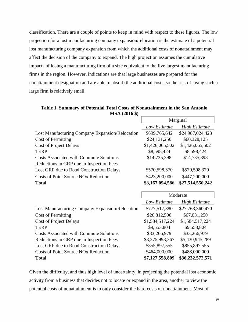
iv
classification. There are a couple of points to keep in mind with respect to these figures. The low
projection for a lost manufacturing company expansion/relocation is the estimate of a potential
lost manufacturing company expansion from which the additional costs of nonattainment may
affect the decision of the company to expand. The high projection assumes the cumulative
impacts of losing a manufacturing firm of a size equivalent to the five largest manufacturing
firms in the region. However, indications are that large businesses are prepared for the
nonattainment designation and are able to absorb the additional costs, so the risk of losing such a
large firm is relatively small.
Table 1. Summary of Potential Total Costs of Nonattainment in the San Antonio
MSA (2016 $)
Marginal
Low Estimate High Estimate
Lost Manufacturing Company Expansion/Relocation $699,765,642 $24,987,024,423
Cost of Permitting $24,131,250 $60,328,125
Cost of Project Delays $1,426,065,502 $1,426,065,502
TERP $8,598,424 $8,598,424
Costs Associated with Commute Solutions $14,735,398 $14,735,398
Reductions in GRP due to Inspection Fees - -
Lost GRP due to Road Construction Delays $570,598,370 $570,598,370
Costs of Point Source NOx Reduction $423,200,000 $447,200,000
Total $3,167,094,586 $27,514,550,242
Moderate
Low Estimate High Estimate
Lost Manufacturing Company Expansion/Relocation $777,517,380 $27,763,360,470
Cost of Permitting $26,812,500 $67,031,250
Cost of Project Delays $1,584,517,224 $1,584,517,224
TERP $9,553,804 $9,553,804
Costs Associated with Commute Solutions $33,266,979 $33,266,979
Reductions in GRP due to Inspection Fees $3,375,993,367 $5,430,945,289
Lost GRP due to Road Construction Delays $855,897,555 $855,897,555
Costs of Point Source NOx Reduction $464,000,000 $488,000,000
Total $7,127,558,809 $36,232,572,571
Given the difficulty, and thus high level of uncertainty, in projecting the potential lost economic
activity from a business that decides not to locate or expand in the area, another to view the
potential costs of nonattainment is to only consider the hard costs of nonattainment. Most of

v
these costs would occur in Bexar County, so to be as conservative as possible, only theses costs
in Bexar County are presented in the following table.
Table 2. Summary of Potential Hard Costs of Nonattainment for Bexar
County (Millions 2016 $)
Marginal
Low Estimate High Estimate
Cost of Permitting $12,700,000 $31,750,000
Cost of Project Delays $897,056,940 $897,056,940
Reductions in GRP due to Inspection Fees $0 $0
Lost GRP due to Road Construction
Delays $458,580,755 $458,580,755
Total $1,368,337,695 $1,387,387,695
Moderate
Low Estimate High Estimate
Cost of Permitting $470,000 $1,175,000
Cost of Project Delays $33,224,331 $33,224,331
Reductions in GRP due to Inspection Fees $89,681,277 $89,681,277
Lost GRP due to Road Construction
Delays $22,929,038 $22,929,038
Total $146,304,646 $147,009,646
The total costs (including both hard and soft costs) by county are provided in Table 3. As
expected, the vast majority of the costs will be absorbed in Bexar County. It is estimated that
costs in Bexar County could range from $2.1 billion to $21.5 billion under a marginal
nonattainment designation. The costs could increase under a moderate nonattainment designation
from $5.3 billion to $28.4 billion. Bandera County is projected to experience the smallest costs
from nonattainment.

vi
Table 3. Total Costs of Nonattainment by County (2016 $)
Marginal
County Low Estimate High Estimate
Atascosa $81,555,999 $595,783,801
Bandera $8,160,646 $230,936,463
Bexar $2,149,208,831 $21,535,495,334
Comal $395,791,302 $1,672,395,202
Guadalupe $405,510,891 $1,956,219,440
Kendall $22,766,034 $404,291,810
Medina $67,637,553 $588,729,702
Wilson $36,463,328 $530,698,487
Total $3,167,094,584 $27,514,550,240
Moderate
County Low Estimate High Estimate
Atascosa $162,142,123 $776,822,557
Bandera $40,135,865 $306,492,259
Bexar $5,267,009,767 $28,443,652,427
Comal $646,923,066 $2,170,715,754
Guadalupe $670,024,508 $2,523,875,813
Kendall $80,931,402 $537,108,519
Medina $147,309,055 $770,004,583
Wilson $113,083,022 $703,900,658
Total $7,127,558,809 $36,232,572,571
NOTE: Differences in the totals compared to Table 1 are due
to rounding.
For comparison purposes, we include data from a September 2015 report on the Potential Costs
of an Ozone Nonattainment Designation to Central Texas – primarily the Austin-Round Rock
metropolitan area (See Table 4). As a regular touchstone for assessing the San Antonio-New
Braunfels MSA performance, the Austin report highlights the differences between the two
economies. The loss of Samsung investment in the Austin-Round Rock area represents a large
portion of the overall costs. On the lower end, abandoning its plans all together represents 78%
of the nearly $24.3 billion estimate while at the higher end of the Austin report’s estimates, this
same project could come to represent 81% of the $41.5 billion estimate. Without diminishing the

vii
importance that such a decision would have for the Austin-Round Rock area, we find that in the
case of the San Antonio area, no single company has the same leverage over economic activity,
at least for the short-term. Not one of our interviews revealed that a company was considering
leaving the area. In fact, our research shows that many larger-scale local companies have taken a
proactive approach toward nonattainment and have already equipped existing and planned
facilities with more environmentally sound technology. However, we find that on-road mobile
sources present a more significant challenge to the area.
Table 4. Overall Economic Impact of Nonattainment Designation from Central Texas
Report 2015 (CAPCOG 2015, 3)
Scenario Low High
Loss of Samsung Expansion ($21,340,142,448) ($33,893,167,418)
Loss of Texas Lehigh Expansion ($1,811,586,399) ($3,700,575,961)
Decker and Sim Gideon Boiler Replacements $0 $0
Transportation Conformity-Routine Analysis ($2,300,000) ($7,000,000)
Transportation Conformity-Routine Project
Delays
($27,407,176) ($41,471,216)
Transportation Conformity-Lapse-Project
Delays
($18,298,801) ($93,012,795)
Transportation Conformity-Loss of Federal
Funds
($23,746,747) ($74,646,101)
General Conformity-Rail Expansion Delays ($7,182,369) ($14,364,738)
General Conformity-Aviation Expansion Delays ($22,449,120) ($44,898,240)
NOx Point Source Emission Reductions ($141,494,537) ($2,047,800,546)
VOC Reductions ($904,917,445) ($1,630,209,506)
TOTAL ECONOMIC IMPACT ($24,299,525,042) ($41,547,146,520)

viii
ACRONYMS AND ABBREVIATIONS
ACRONYM OR
ABBREVIATION
DEFINITION
CAA Clean Air Act
CBSA Core-Based Statistical Area
CSA Combined Statistical Area
CTG Control technique guideline
EPA U.S Environmental Protection Agency
FHWA Federal Highway Administration
FTA Federal Transit Administration
HAP Hazardous air pollutant
I/M Inspection and monitoring
LAER Lowest achievable emission rate
NA Nonattainment
NAAQS National Ambient Air Quality Standards
NNSR Nonattainment New Source Review
NOx Nitrogen oxide (NO and NO2)
NSR New Source Review
PAL Plant-wide applicability limit
PSD Prevention of significant deterioration
RACM Reasonably achievable control measures
RACT Reasonably achievable control technology
RFG Reformulated gasoline
RFP Reasonable further progress
SIP State Implementation Plan
SOCMI Synthetic Organic Chemical Manufacturing Industry
TCEQ Texas Commission on Environmental Quality
TCM Transportation control measures
TXDOT Texas department of Transportation
TXLED Texas Low-Emission Diesel
VOC Volatile organic compounds

1
1. Introduction to EPA’s New Ozone Standard (October 1, 2015)
To meet its obligations under the Clean Air Act (CAA) as amended in 1990, the EPA has
established air quality standards in 40 CFR Part 50. In these regulations, the EPA establishes the
National Ambient Air Quality Standards (NAAQS) to promote and sustain healthy living
conditions. Primary NAAQS are established to protect public health, and secondary NAAQS are
established to protect public welfare by safeguarding against environmental and property damage
(Table 1.1). These standards define acceptable ambient air concentrations for six criteria air
pollutants: nitrogen dioxide (NO2), ozone (O3), sulfur dioxide (SO2), carbon monoxide (CO),
lead (Pb), and particulate matter (including PM10 and PM2.5).
Table 1.1 National Ambient Air Quality Standards (NAAQS) (from EPA, 2016a)
Pollutant Primary/Secondary Averaging Time Level Form
Carbon Monoxide Primary 8-hour 9 ppm Not to be exceeded more
than once per year 1-hour 35 ppm
Lead Primary/Secondary Rolling 3 mo.
avg 0.15 μg/m3 Not to be exceeded
Nitrogen Dioxide Primary 1-hour 100 ppb
98th percentile of 1-hour
daily maximum
concentrations, averaged
over 3 years
Primary/Secondary Annual 53 ppb Annual Mean
Ozone
Primary/Secondary 8-hour 70 ppb
(2015)
Annual fourth-highest
daily maximum 8-hour
concentration, averaged
over 3 years
Primary/Secondary 8-hour 75 ppb
(2008)
Remains in effect in
some areas.
Particulate
Matter
PM2.5
Primary Annual 12.0 μg/m3 annual mean, averaged
over 3 years
Secondary Annual 15.0 μg/m3 annual mean, averaged
over 3 years
Primary/Secondary 24-hour 35 μg/m3 98th percentile, averaged
over 3 years
PM10 Primary/Secondary 24-hour 150 μg/m3
Not to be exceeded more
than once per year on
average over 3 years

2
Sulfur Dioxide
Primary 1-hour 75 ppb
99th percentile of 1-hour
daily maximum
concentrations, averaged
over 3 years
Secondary 3-hour 0.5 ppm Not to be exceeded more
than once per year
EPA requires states to monitor ambient air quality and evaluate compliance with respect to the
NAAQS. Based on these evaluations, EPA characterizes the air quality within a defined area
with respect to each of the six criteria air pollutants using a compliance-based classification
system. Defined areas range in size from portions of cities, to metropolitan statistical area (MSA
as defined by the U.S. Bureau of the Census), to large regions composed of many counties. For
areas that are in attainment, levels for a given criteria air pollutant are below the NAAQS, while
areas that are in nonattainment have air quality that exceeds the NAAQS. For those areas where
there is insufficient available information for classification purposes, a status of
unclassifiable/attainment is assigned. An ozone nonattainment classification can be further
defined as
Marginal,
Moderate,
Serious,
Severe, or
Extreme
based on the degree to which the NAAQS is exceeded (Table 1.2).

3
The ozone nonattainment classification
for a given area determines the planning
and control requirements that will be
imposed to improve the regional air
quality and move the area towards
attainment status. If an area is
designated as nonattainment, then the
state must develop (a process that involves public review and comment) revisions to the State
Implementation Plan (SIP) that demonstrate how the state plans to bring the area back into
attainment status. The SIP revision will require different elements depending on the
nonattainment classification.
On October 26, 2015, EPA issued a final rule to revise the primary eight-hour NAAQS for
ground-level ozone from 0.075 parts per million (ppm) (2008 standard) to 0.070 ppm, or 70 parts
per billion (ppb). The EPA also revised the secondary NAAQS for ozone to 70 ppb, equivalent
to the primary standard (EPA, 2015a; 80 Fed. Reg. 65,291). The final rule became effective on
December 28, 2015, although the 2008 ozone standard remains in effect in some areas; for
permitting purposes, the most stringent classification will control when two separate standards
apply. Transitioning of these areas to the 2015 ozone standard will be addressed in the
implementation rule for the current standard.
With the issuance of the new ozone standard, the EPA also required that the governor of each
state must recommend designations of attainment, nonattainment, or unclassifiable under the
2015 8-hour standard for all areas of the state within one year (i.e., by October 1, 2016). The
Texas Commission on Environmental Quality (TCEQ) issued its recommendations to the
governor on August 3, 2016 (TCEQ, 2016a). Under these recommendations, Bexar County
would be designated as nonattainment with respect to ozone, but the degree of nonattainment
(e.g., Marginal to Extreme) is not identified. The EPA's final decision on nonattainment area
boundaries could include counties or parts of counties within an MSA, Combined Statistical
Table 1.2. 8-Hour Design Values for the 2015
Ozone NAAQS of 70 ppb (from EPA, 2016a,b)
Area Class 8 hour design value (ppb)
Marginal ≥70 to < 81
Moderate ≥ 81 to < 93
Serious ≥ 93 to < 105
Severe-15 ≥ 105 to < 111
Severe-17 ≥ 111 to < 163
Extreme ≥ 163

4
Area (CSA), or Core-Based Statistical Area (CBSA) or other counties that EPA determines
contribute significantly to the nonattainment.
For the purposes of this summary report, it is assumed that the 8-county region that comprises
the San Antonio MSA would be classified as either marginal or moderate nonattainment with
respect to the 2015 ozone NAAQS. It is not anticipated that the region would receive one of the
more serious nonattainment classifications.
2. Background on Nonattainment Area Requirements
Ground-level ozone is not produced through direct emissions. Instead, this ozone is created
indirectly by photochemical reactions involving precursor emissions of NOx and volatile organic
compounds (VOC) in the presence of sunlight. Along with natural sources, these precursor
chemicals are produced by a wide variety of human activities such as vehicle exhaust, power
plants, industrial boilers, refineries, chemical plants, and other industrial operations, making it
challenging to identify a single source of emissions. In addition, the complex photochemical
reactions that produce ozone vary with local atmospheric conditions such as temperature, and
seasonal and daily weather patterns. For example, ozone tends to be highest on hot, sunny days,
although certain cold weather air conditions such as temperature inversions can lead to higher
ozone levels. Ozone can also be transported by wind, leading to the impairment of air quality in
rural areas that are downwind from urban centers that have higher levels of NOx and VOC that
result from human activity (EPA, 2014).
2.1. Overview of Nonattainment Area Requirements
As discussed previously, TCEQ issued its recommendations for area designations with respect to
the 2015 eight-hour ozone rule on August 3, 2016 (TCEQ, 2016). TCEQ's recommended
designation status for the eight-county study area is identified in Table 2.1.

5
The recommended designation of Bexar County
as nonattainment is based on design values
calculated using certified 2013 through 2015
eight-hour ozone data for Texas counties with
regulatory monitors (TCEQ, 2016a, Attachment
B). The 2015 certified design value for Bexar
County was 78 ppb, slightly less than Harris (79
ppb) and Tarrant (80 ppb) in the Houston and
Dallas areas. The final EPA designation is
anticipated to be based on 2014 – 2016 8-hour ozone data (TCEQ, 2016j), which yields a design
value of 73 ppb for Bexar County.
Depending on the nonattainment designation, a number of different requirements are imposed
with the goal of improving the affected air quality and returning to attainment status. Each
increased level of nonattainment (i.e., as air quality impairment becomes more severe, or the area
is unable to meet the NAAQS by the attainment date associated with a lower nonattainment
classification), incorporates all of the requirements for the lower levels of nonattainment, and
adds additional requirements. The result is that the number of requirements for air quality
improvement and the associated costs of implementation can increase markedly as regional air
quality is degraded. These requirements are established through revisions to the SIP, and for
ozone nonattainment, the required SIP elements by nonattainment classification include (EPA,
2016h):
Marginal (3 years to attain):
Baseline emission inventory, followed by periodic updates
New source review (NSR) program
o NSR offset ratio 1.1:1
Major source emission statements
o Major source threshold 100 tons per year (tpy), and
Table 2.1 TCEQ 2015 Eight-Hour Ozone
NAAQS Designation Recommendations
(from TCEQ, 2016a)
County TCEQ Recommended
Designation (8/3/2016)
Atascosa Unclassifiable/Attainment
Bandera Unclassifiable/Attainment
Bexar Nonattainment
Comal Unclassifiable/Attainment
Guadalupe Unclassifiable/Attainment
Kendall Unclassifiable/Attainment
Medina Unclassifiable/Attainment
Wilson Unclassifiable/Attainment

6
Transportation conformity demonstration
Moderate (6 years to attain):
All requirements for Marginal classification, with
o Major source threshold 100 tpy
o NSR offset ratio 1.15:1
Major source (VOC/NOx) reasonably available control technology (RACT)
Attainment demonstration
15% reasonable further progress (RFP) over 6 years
Basic vehicle inspection and maintenance (I/M) program
Contingency measures for failure to attain
Stage II gasoline vapor recovery (Note: With the development of on-board vapor
recovery technology, EPA determined that Stage II vapory recovery was no longer
required and could be removed from state SIPs. EPA approved the revisions to the Texas
SIP removing Stage II vapor recovery in April 2014, and gasoline stations were allowed
to begin decommissioning Stage II equipment in May 2014 (TCEQ, 2016l).
The following is a brief listing of the controls and requirements that are imposed as a function of
nonattainment status (EPA, 2016c,d,e). Examples of controls applied in Texas nonattainment
areas are provided in Appendix A for the initial (July 20, 2012) Marginal designation of the
Houston-Galveston-Brazoria MSA (designated as Moderate relative to the 2008 ozone standard
on December 14, 2016) and the Dallas-Fort Worth MSA (Moderate):
Nonattainment (Marginal, 3 years to attain):
o Marginal area nonattainment new source review (NNSR) permitting rules;
o Transportation Conformity;
o General Conformity;
o Emissions Inventory; and
o Emission Statements;
Nonattainment (Moderate, 6 years to attain):
o All Marginal area requirements;
o Moderate area NNSR permitting rules;

7
o NSR offset of 1.15:1
o Attainment demonstration;
o Reasonable further progress (RFP) demonstration (15% reduction in VOC
emissions);
o Reasonably available control technology (RACT) for major sources of NOx;
o RACT for major sources of VOC;
o RACT for VOC sources covered by an EPA control technique guideline (CTG)
document;
o Contingency measures for attainment and RFP; and
o A basic vehicle inspection and maintenance (I/M) program;
Nonattainment (Serious, 9 years to attain):
o All Marginal and Moderate area requirements;
o Serious area NNSR permitting rules;
o Enhanced I/M program;
o Enhanced monitoring;
o Clean Fleet program;
o Transportation control measures (TCMs) to offset growth in vehicle miles
traveled; and
o Additional 3% per year reduction in NOx and VOC emissions for RFP;
Nonattainment (Severe, 15/17 years to attain):
o All Marginal, Moderate, and Serious area requirements;
o Severe area NNSR permitting;
o An emissions fee program if the area fails to attain its standard by its attainment
deadline; and
o Additional 3% per year reduction in NOx and VOC emissions for RFP;
Nonattainment (Extreme, 20 years to attain):
o All Marginal, Moderate, Serious, and Severe area requirements;
o Extreme area NNSR permitting;
o Clean Fuel for Boilers; and
o Additional 3% per year reduction in NOx and VOC emissions for RFP

8
If the air quality in an area that has been previously designated as nonattainment improves to
meet the NAAQS, the area will be identified as a maintenance area. It is important to consider
that even if the regional air quality is improved and achieves a designation of maintenance, the
requirements will remain in effect until continued NAAQS compliance can be demonstrated. A
general timeline is presented in Figure 2.1 with estimated dates relevant to a nonattainment
designation for the San Antonio region given in Table 2.2.
Figure 2.1. Overview of CAA Ozone Planning & Control Requirements by Classification
(from EPA, 2015b)

9
Table 2.2. A general timeline for NAAQS compliance (Modified from TCEQ, 2016j, CAPCOG, 2015)
October 2015 New Primary Ozone Standard: 70 ppb; Secondary standard same as
primary (EPA, 2015a)
August 2016 TCEQ makes recommendations to governor for nonattainment
designations (TCEQ, 2016a)
October 2016 State designation recommendations due to EPA
November 2016 EPA proposes implementation rule (EPA, 2016b)
June 2017 EPA sends letter to states with proposed nonattainment area
designations
October 2017 EPA to sign (finalize) designations and classifications; EPA to finalize
implementation rule
October 2019 Emissions Inventory State Implementation Plan (SIP) revisions due for
all nonattainment areas
October 2020-2021 Attainment Demonstration SIP revisions due
Once the SIP revisions are proposed and approved, and the implemented programs are able to
improve air quality to meet the 2015 ozone NAAQS, then nonattainment areas are eligible for
redesignation. In accordance with the provisions of Section 175 of the CAA, TCEQ would
propose a maintenance plan and prepare an attainment redesignation request that would be
forwarded to EPA, with up to two years for EPA to consider the requests. If EPA approves the
maintenance plan and the redesignation request, then there will be a 10-year maintenance period
to ensure that improved air quality can be sustained. Approximately two years before the end of
this period, TCEQ will prepare a second 10-year maintenance plan for EPA review and approval.
In summary, the designation of an area (or areas) as nonattainment with respect to the ozone
NAAQS can result in required controls, analysis, modeling, and monitoring that can cover a
period of regulatory oversight that extends from years to decades.
2.2. Nonattainment New Source Review
Nonattainment New Source Review (NNSR) is required for applicants seeking permits to either
construct a new major stationary source or install major modifications to an existing major
source in a nonattainment area. For NNSR permitting in Marginal and Moderate ozone
nonattainment areas, a major source is defined as a facility that has the potential to emit at least
100 tpy of either NOx or VOC, while a major modification is considered to be a physical
modification or change in operations that would increase emissions of NOx or VOC by at least
40 tpy. The numerical criteria for these definitions are based on the conservative assumption that

10
a facility is running at 100 percent capacity for 24 hours/day and 365 days/year. A permit that is
under consideration as part of an NNSR cannot be approved unless the review determines that a
number of location-specific requirements intended to minimize the effects on air quality from the
proposed facility or modifications can be met.
TCEQ identifies the types of facilities that often require NNSR (TCEQ, 2016d) (Table 2.3):
Table 2.3. List of facilities, as defined by the Texas Clean Air Act § 382.003(6), typically found at
sources that need New Source Review permits (from TCEQ, 2016d). Abrasive Blasting Operations Glycol Dehydrator
Absorbers Grain Elevators
Adsorption Systems Hot Mix Asphalt Plants
Anhydrous Ammonia Storage and Handling Incinerators
Asphalt Processing and Asphalt Roofing Manufacturing Internal Combustion Engines
Boilers Iron and Steel Industry
Bulk Gasoline Terminals Liquid Storage Terminals
Bulk Material Handling Loading Operations
Chrome Plating and Anodizing Operations using Chromic Acid Metallizing-Metal Spraying Operations
Coating Manufacturing Operations Oriented Strandboard Mills
Concrete Batch Plants Painting Operations
Cooling Towers Petroleum Coke Storage and Transfer
Cotton Gins Plant Fuel Gas (Under Review)
Degreasing Operations Polyethylene and Polypropylene Manufacturing
Drum Filling Printing Operations
Dry Bulk Fertilizer Handling Process Furnaces and Heaters (Under Review)
Equipment Leak Fugitives Process Vents
Ethylene Oxide Sterilization Units Rock Crushing Plants
Fiber Reinforced Plastics and Cultured Marble Storage Tanks
Flares and Vapor Combustors Sulfur Recovery Units
Fluid Catalytic Cracking Units Truck or Railcar Cleaning
Galvanizing Operations Turbines
Glass Manufacturing Vapor Oxidizers
Wastewater
According to the EPA, all NNSR programs “…have to require (1) the installation of the lowest
achievable emission rate (LAER), (2) emission offsets, and (3) opportunity for public
involvement.” (EPA, 2016f).
LAER focuses on setting the emissions limits on new or modified major sources in
nonattainment areas. For the purposes of NNSR review, LAER will focus on the most stringent
limitations from either of the following:

11
The most stringent emissions limitation, which is contained in the SIP, for a class or
source category, unless the owner or operator of the source demonstrates that such
limitations are not achievable; or
The most stringent emissions limitation that is achieved in practice by a class or source
category. This limitation, when applied to a modification, means the lowest achievable
emissions rate for the new or modified facilities.
The LAER requirements that are established as part of the NNSR may be achieved by a
combination of methods that could include changes to raw materials, process modifications, or
add-on controls. Depending on the specific technologies or processes involved, these methods
may increase the cost of either building a new facility that qualifies as a major source, or
expanding operations of an existing major source within a nonattainment area. In addition, a
typical NNSR includes permitting fees ($75,000 maximum) as well as an extensive review
process that can add to facility cost. For example, according to the voluntary TCEQ Expedited
Permitting Program (TCEQ, 2016e), the NNSR permitting process can include the additional
upfront costs in the form of surcharges above and beyond the costs associated with preparing the
permit application:
New Source Review (NSR) case-by-case permit - $10,000
Federal NSR permits [Prevention of Significant Deterioration (PSD) including
greenhouse gas PSD, Nonattainment (NA), Plantwide Applicability Limit (PAL), and
Hazardous Air Pollutant (HAP)] - $20,000
Basic steps for the TCEQ NSR permit program (TCEQ, 2016e), include:
Pre-Application: This step includes a pre-application meeting, prior to submitting the
permit application package. The purpose of this meeting is to establish a general
schedule for the permit application review. Prior to the meeting, the applicant submits

12
o An overview of the project, including a description of the processes involved and the
types of emissions (contaminants and approximate quantities);
o A discussion of federal applicability including netting evaluation, if applicable;
o A discussion of best available control technology (BACT);
o A list of permitting questions to resolve in the meeting (BACT, impacts review
strategies, calculation methodology, rule applicability, etc.);
o A draft application and modeling protocol, if available; and
o Anticipated submittal date and project timing (e.g., start of construction).
Draft Application: An early draft of the application is made available to the TCEQ staff
for preliminary evaluation of the application and air dispersion modeling protocols. This
draft is to be submitted at least three weeks prior to the planned, formal application
submittal. The TCEQ staff then has seven days to provide feedback on deficiencies, if
any, that they identify in the draft. The applicant has the opportunity to resolve these
deficiencies prior to submitting the formal application.
Application Submittal: After resolving deficiencies and questions from the TCEQ staff
on the draft application and the proposed modeling, the applicant submits the formal
application electronically, along with the appropriate surcharge as identified previously.
If deficiencies are not addressed, then the application may be voided.
Enhanced Administrative Review: After receiving the formal application and modeling
results prepared by the applicant, TCEQ staff conducts a review and identifies any
deficiencies. These are communicated to the applicant who has 10 days to respond. The
staff will then review the responses – if the responses are not acceptable, then the
application will be voided.
Technical Review: – If the applicant’s responses to the EAR are acceptable, the TCEQ
conducts a technical review. The review includes proposed control technologies (Best
Available Control Technologies (BACT) or LAER in the case of NNSR), modeling
calculations, federal applicability, and technical completeness. The TCEQ review will
13
verify emission rates, and request a complete Air Quality Analysis (AQA) that follows
the approved modeling protocol. As with other steps, TCEQ may void the application if
the applicant does not provide complete and accurate information within the specified
timeframe
Modeling Audit: The TCEQ Air Dispersion Modeling Team (ADMT) conducts an audit
of the modeling results in the context of the agreed upon modeling protocols. The air
dispersion modeling must pass the modeling audit two times, or the permit application
may be voided. If there are potential public health effect implications, additional impact
reviews may need to be conducted by the TCEQ Toxicology Division, with additional
time necessary to complete the permit application review
Draft Permit: If the application passes these review steps, the TCEQ permit reviewer will
provide a draft permit (with conditions), triggering a 30-day public comment period.
Written comments are addressed by the permit reviewer, and the draft permit is updated
as necessary. If a public hearing request is received within the initial 3-day period, the
applicant may be required to undergo a second 30-day public notice period.
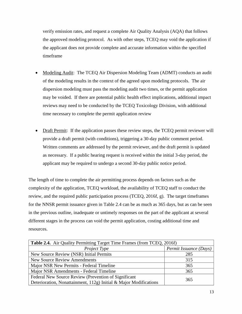
The length of time to complete the air permitting process depends on factors such as the
complexity of the application, TCEQ workload, the availability of TCEQ staff to conduct the
review, and the required public participation process (TCEQ, 2016f, g). The target timeframes
for the NNSR permit issuance given in Table 2.4 can be as much as 365 days, but as can be seen
in the previous outline, inadequate or untimely responses on the part of the applicant at several
different stages in the process can void the permit application, costing additional time and
resources.
Table 2.4. Air Quality Permitting Target Time Frames (from TCEQ, 2016f)
Project Type Permit Issuance (Days)
New Source Review (NSR) Initial Permits 285
New Source Review Amendments 315
Major NSR New Permits - Federal Timeline 365
Major NSR Amendments - Federal Timeline 365
Federal New Source Review (Prevention of Significant
Deterioration, Nonattainment, 112g) Initial & Major Modifications 365

14
2.3. Conformity
Conformity, established under Title I, Section 176 of the CAA, is a provision that applies to
NAAQS nonattainment and maintenance areas and mandates that all federal actions conform to
(i.e. meet) the requirements of an approved SIP. For conformity purposes, a federal action
includes not just federal agency engagement in specific activities, but also federal actions that
provide “…support in any way, or provide financial assistance for, license or permit, or approve,
any activity that does not conform to an implementation plan…” Federal actions are evaluated
as part of a conformity determination prior to proceeding with a given action. The purpose of
conformity is to eliminate or reduce violations of the NAAQS and achieve attainment of these air
quality standards. Specifically, conforming activities or actions should not cause or contribute to
new violations, increase the frequency or severity of existing violations, or delay timely
attainment of any standard or interim emission reductions.
Conformity requirements are categorized according to transportation and general conformity,
under EPA regulations 40 CFR Part 93. Transportation conformity requirements apply to
transportation plans, transportation improvement programs, and highway and transit projects
funded or approved by the Federal Highway Administration (FHWA) and the Federal Transit
Administration (FTA) (40 CFR Part 93, Subpart A). General conformity requirements apply to
all federal actions in nonattainment and maintenance areas not covered by the transportation
conformity rule (40 CFR Part 93, Subpart B).
2.3.1. Transportation Conformity
Section 176(c)(6) of the CAA and the conformity regulation at 40 CFR § 93.102(d) provide a
one-year grace period from the effective date of designation before transportation conformity
applies in areas newly designated as nonattainment for any of the transportation-related NAAQS
(ozone, particulate matter, nitrogen dioxide, and/or carbon monoxide) (EPA, 2012). During this
grace period, a transportation conformity determination for the region must be completed and
submitted to local, state, and federal consultative agencies for review, with the FHWA and FTA
providing final approval. In addition, long-term metropolitan transportation plans (MTPs) and

15
shorter-term transportation improvement programs (TIPs) that are funded in part by federal
transportation agencies such as the FHWA and FTA would need to be revised to include an
analysis of the potential impact of the plans on regional air quality to demonstrate that the
activities “conform to” the SIP (Figure 1). The element of the SIP to which a transportation
conformity demonstration must conform is the motor vehicle emission budget (MVEB), which is
a representation of an area’s projected regional on-road mobile source emissions in the SIP for
NAAQS-related pollutants. With respect to the ozone NAAQS, a transportation conformity
determination would need to demonstrate that future emissions of ozone precursors (NOx and
VOC) resulting from an area’s MTP and TIP would be equal to or less than the MVEB included
in the SIP and approved by EPA. The metropolitan planning organization (MPO) in a
nonattainment or maintenance area is typically responsible for completing and submitting
transportation conformity demonstrations.
Transportation conformity demonstrations are to be made at least every four years, but can occur
more frequently if the MTP and TIPs are updated more frequently (FHWA, 2010). If, after the
initial nonattainment designation, transportation conformity is not demonstrated and approved by
FHWA and FTA, then after a one-year grace period, the region is considered to enter into a
conformity “lapse”, and federal funds for highway and transit improvements can be restricted.
During a lapse, only a limited number of transportation projects can proceed, including:
Exempt projects such as
o Safety improvements,
o Road maintenance,
o Rehabilitation, or
o Certain mass transit, bicycle/pedestrian, mass transit, carpool/vanpool projects that
can be shown to not have a negative impact on the region’s air quality;
Transportation Control Measures (TCM)s in approved SIPs; and
Projects or project phases that are already authorized.
Also, during a conformity lapse, no new non-exempt projects can be amended into the MTP or
TIP.

16
Figure 2.2. Simplified version of the transportation conformity process for metropolitan
transportation plans/TIPs and projects (from FHWA, 2010).
For the San Antonio region, the Alamo Area Metropolitan Planning Organization (AAMPO) is
the independent local agency that provides direction for the allocation of federal funding for
urban transportation planning. In this role, the AAMPO develops and updates the MTP and TIPs

17
for the region (AAMPO, 2015, 2016a,c). If the region is designated as nonattainment with
respect to ozone, then the AAMPO would have the primary responsibility for demonstrating
transportation conformity for the MTP, TIPs, and other regionally significant projects. For the
purposes of the AAMPO (AAMPO, 2016b), regionally significant projects are those that include
Roadways that are federally functionally classified as interstate freeways, other freeways,
or principal arterials
Roadways and intermodal connectors included in the federally adopted National
Highway System
Roadways designated as State Highways or US Highways
Fixed guideway transit facilities
Since demonstrating transportation conformity would require consultation with federal, state, and
local agencies, it could potentially add time and cost to transportation planning. For example,
currently, the TIP is updated every two years and amended quarterly, but if the region is
designated as nonattainment with respect to ozone, then the need for interagency consultation
and public outreach would potentially reduce the frequency of the amendments and updates.
Conformity would also be considered at the project level, where a project must be demonstrated
to come from a conforming MTP and TIP, with a design and scope that has not changed
significantly from the conforming plans, and addresses potential localized emissions impacts.
With respect to potential ozone nonattainment designation for the San Antonio region, the
working schedule assumptions for the AAMPO (AAMPO, 2016a) are:
Oct 2015: EPA Ozone NAAQS Final Rule – 70 ppb standard
Oct 2016: Governors propose nonattainment areas –
o TCEQ proposed Bexar County only
Oct 2017: EPA designates nonattainment areas
Dec 2017 to June 2018: AAMPO Develops Metropolitan Transportation Plan (MTP),
Transportation Improvement Program (TIP), Conformity Document and conducts public
involvement process

18
June 2018: Consultative Partners to Receive MTP, TIP and Conformity Documents
Oct 2018: Transportation Conformity Determination Due
If the conformity determination cannot be completed and approved to meet the October 2018
deadline, then the region would be considered to be in conformity lapse, and the requirements
discussed previously would apply.
2.3.2. General Conformity
General conformity determinations are performed on a project-by-project basis in NAAQS
nonattainment and maintenance areas for actions that are federally funded, licensed/permitted, or
requires federal agency approval and is not covered by transportation conformity regulations.
The federal agency proposing an activity would work with state and local governments to
evaluate whether potential activity-related impacts to air quality would conform to the SIP based
on regulations in 40 CFR Parts 6, 51, and 93 (EPA, 1993).
In the first step of the process, the federal agency evaluates a proposed project to assess the
applicability of general conformity requirements. In making this evaluation, the agency assesses
whether:
The proposed activity is exempt from general conformity requirements (40 CFR §
93.153(c))
The proposed activity is “presumed to conform” (40 CFR § 93.153(g))
Total direct and indirect emissions are below the de minimis level. For the ozone
NAAQS, emissions from ozone precursors determine whether general conformity must
be demonstrated for an action, with de minimis levels of 100 tons per year of NOx or
VOC for Marginal and Moderate nonattainment areas and for maintenance areas)
If the proposed activity meets any of these criteria, then a general conformity analysis is
complete and a detailed determination and analysis is not required. If these criteria are not met,
then general conformity requirements are applicable, and the agency will determine whether:

19
The affected facility meets an emissions budget approved by the state as part of the SIP
The action meets all state control requirements
The action would cause a new violation of the standard or interfere with timely
attainment, maintenance, or reasonable further progress
Total and indirect emissions are specifically identified and accounted for in the SIP
The state/local air quality agency has provided a written statement that emissions from
the project, together with other emissions in the nonattainment/maintenance area will not
exceed the SIP emissions budget
As necessary, the proposing federal agency may obtain emissions offsets to ensure that there is
no net increase in emissions for the nonattainment or maintenance area. Offsets would occur
during the same calendar year as any emissions increase from the proposed action, unless the
proposed offsets exceed a ratio to the anticipated emissions of:
1.15-to-1 for Moderate nonattainment areas
1.1-to-1 for Marginal and maintenance areas.
For the purposes of a general conformity analysis, direct emissions are those emissions that are
caused/initiated by the proposed federal action, and occur at the same time and place within
nonattainment area. As the name suggests, indirect emissions are those reasonably foreseeable
emissions that are caused/initiated by the proposed federal action, but occur in a different time
and place within the nonattainment area. Indirect emissions are further limited to those that the
federal agency can “practically control” and for which the agency can maintain control through
continuing program responsibility (FAA/EPA, 2002).
2.4. Reasonably Available Control Technology
Should the San Antonio region be classified as a Moderate or higher ozone nonattainment area,
sources of emissions within the area will need to demonstrate that they have implemented
Reasonably Available Control Technology (RACT). Existing facilities would need to be

20
retrofitted with pollution control technology, with RACT defined under 40 CFR § 51.100(o) as
“…devices, systems, process modifications, or other apparatus or techniques that are reasonably
available, taking into account: (1) the necessity of imposing such controls in order to attain and
maintain a national ambient air quality standard; (2) the social, environmental, and economic
costs of such controls; and (3) alternative means of providing for attainment and maintenance of
such standard.”
For ozone nonattainment areas, there are three categories of RACT:
VOC RACT for sources covered by an EPA Control Technique Guideline (CTG)
document
Non-CTG major source VOC RACT, including emission sources covered in an EPA
Alternative Control Technology (ACT) document
Major source NOx RACT
The EPA defines RACT as the lowest emission limitation that a particular source is capable of
meeting by the application of control technology that is reasonably available, considering
technological and economic feasibility (EPA, 2016g). In Texas, RACT requirements for ozone
established by TCEQ are contained in 30 TAC Chapters 115 (VOC) and 117 (NOx), and are
adopted in the Texas SIP. TCEQ applies these requirements to reduce emissions from existing
sources regardless of construction authorization or date of construction for the source (TCEQ,
2011).
2.5. Reasonable Further Progress
Should all or part of the San Antonio region be classified as nonattainment-Moderate with
respect to ozone, the CAA requires that the state (TCEQ in this case) submit plans that show
reasonable further progress (RFP) towards achieving attainment.
TCEQ would be required to submit an RFP analysis as a revision to the SIP for the
nonattainment area within three years of the effective date for the nonattainment designation.

21
The RFP SIP revision would not be required to demonstrate the attainment of the NAAQS ozone
standard, but would instead, as specified in Section 182(c)(2) of the CAA and in 40 CFR
§51.910, involve reducing ozone precursor emissions (NOx and/or VOC) at annual increments
between the baseline year and the attainment year. For example, a RFP SIP revision prepared for
the moderate nonattainment classification for the Dallas-Fort Worth (DFW) 10-county area
included control strategies to achieve reductions in VOC and/or NOx, as well as annually
updated MVEB inventories, transportation modeling, and quantification of control strategies,
with milestones for each year of the RFP analysis to demonstrate that the proposed control
strategies would result in a reduction of 15% in emissions for the ozone precursors (VOC and/or
NOx) within six years after designation (TCEQ, 2015a). Examples of the control strategies
considered for the DFW RFP analysis are included in Table 2.5.
2.6. Vehicle Inspection and Maintenance
(I/M) Programs
Vehicle inspection and maintenance (I/M)
programs have been used for many years to
improve air quality for NAAQS criteria
pollutants related to vehicle emissions (CO,
Ozone through its precursors NOx and VOC).
I/M programs use special equipment to
measure the pollution in a vehicle’s exhaust,
identifying high-emitting vehicles, and
causing them to be repaired.
For areas designated as Moderate
nonattainment or higher with respect to
ozone, the CAA establishes basic I/M
programs. Specifically, under 40 CFR §
51.350(a)(4), “…any area classified as a moderate ozone nonattainment area, and not required to
implement enhanced I/M under paragraph (a)(1) of this section, shall implement basic I/M in any
Table 2.5. Summary of DFW NOx and VOC Cumulative
Emissions Reductions from Control Strategies (from
TCEQ, 2015a)
Chapter 117 NOx point source controls
Chapter 115 storage tank rule
Coating/printing rules
Portable fuel container rule
Federal Motor Vehicle Control Program
Inspection and maintenance (I/M)
Reformulated gasoline (RFG)/ East Texas Regional Low Reid
Vapor Pressure Gasoline Program
On-road Texas low emission diesel (TxLED)a
Tier 1 and 2 locomotive NOx standards
Small non-road spark ignition (SI) engines (Phase 1)
Heavy duty non-road engines
Tiers 2 and 3 non-road diesel engines
Small non-road SI engines (Phase 2)
Large non-road SI and recreational marine
Non-road TxLED
Non-road RFG
Tier 4 non-road diesel engines
Diesel recreational marine
Small SI (Phase 3)
Chapter 117 NOx area source engine controls
Drilling rig low emission diesel
2017 Low Sulfur Gasoline Standard aTXLED required in 5 of the 8 counties considered in this
report (Atascosa, Bexar, Comal, Guadalupe, and Wilson)
(TCEQ, 2016k)

22
1990 Census-defined urbanized area with a population of 200,000 or more.” Additionally, 40
CFR § 51.350(b)(2) specifies that, “outside of ozone transport regions, programs shall nominally
cover at least the entire urbanized area, based on the 1990 census. Exclusion of some urban
population is allowed as long as an equal number of non-urban residents of the MSA containing
the subject urbanized area are included to compensate for the exclusion.” Therefore, with
respect to the potential nonattainment designation of the San Antonio area, not all of the counties
in the eight-county area considered in this study would necessarily be required to have a vehicle
I/M program. If the area were to be classified as higher than Moderate, additional I/M
requirements in 40 CFR §51.350 could apply and require implementation of an I/M program in
other parts of the nonattainment area.
In establishing the basic I/M program, the CAA identified EPA as the agency responsible for
developing the performance standards to be met. EPA has revised the I/M performance
standards several times to give greater flexibility to nonattainment regions in designing their I/M
programs and to meet revisions to the NAAQS ozone standards. Although there is flexibility in
designing I/M programs, common methods include visual inspection, emissions testing, and/or
accessing the onboard diagnostic computer codes from 1996 and newer vehicles (EPA, 2006).
States can perform testing in a variety of ways, including centralized test-only inspection facility
(State- or contractor-operated), or at privately owned and operated decentralized facilities using
certified mechanics. If a vehicle does not pass the test, then it is required to be repaired before it
can continue to be operated in the area. In Texas, for those nonattainment regions with I/M
programs, the programs are integrated with the annual safety inspection program and operated by
the Texas Department of Public Safety (DPS) in conjunction with TCEQ (TCEQ, 2016h). The
components of existing Texas I/M programs include:
Motorists must successfully pass both the emissions and safety portions of the inspection
prior to receiving a vehicle inspection report, which will be used to obtain a vehicle
registration sticker.
Gasoline vehicles model-year 2 through 24 years old are inspected annually beginning
with the vehicle's second anniversary.

23
Remote sensing element randomly inspects vehicles emissions on highways.
All inspections are collected at a central database.
Recognized Emission Repair Facilities ensure quality repair of vehicles.
Waivers and time extensions are available for eligible vehicle owners.
The SIP must be revised to include the implementation of a basic I/M program, and the revisions
must be reviewed, approved, and overseen by EPA. The I/M program is required to gather test
data on individual vehicle tests (including tracking Vehicle Identification Numbers or VINs) as
well as quality control data on testing equipment. The I/M program is also required to report I/M
program results related to test data, quality assurance, quality control and enforcement.
2.7. Attainment Demonstration
Areas that are classified as Moderate nonattainment or higher with respect to ozone require a
demonstration that the area will be able to achieve attainment by the attainment date. The
demonstration is accomplished by computer simulations of ozone levels during the last complete
ozone season prior to the attainment date. The demonstration also must include evidence that the
state has implemented reasonably available control measures (RACM) necessary to advance
attainment as well as any additional measures that would be implemented if attainment was not
achieved by the established date. Basic ideas of RACM include the following types of criteria
for control measures:
Technologically feasible;
Economically feasible;
Does not cause “substantial widespread and long-term adverse impacts;
Is not “absurd, unenforceable, or impractical;” and
Can advance the attainment date by at least one year
As with other measures to improve regional air quality, the SIP is revised to include the RACM
used to demonstrate attainment, and submitted for review and approval by EPA. The SIP

24
revision is due within 36 months of an initial nonattainment designation for newly designated
Moderate ozone nonattainment areas.
2.8. Anti-Backsliding Requirements
When an area is designated as nonattainment with respect to NAAQS, existing rules, controls,
and practices that are incorporated into the approved SIP revisions for that area cannot be
relaxed, regardless of changes to the NAAQS, until the air quality improves to restore attainment
status for the region. Requirements known as anti-backsliding requirements are imposed to
ensure air quality in nonattainment areas will not worsen. EPA is prohibited by the Clean Air
Act from approving a revision to the SIP that proposes actions that would interfere with progress
towards attainment, and once an attainment designation is achieved, the state must be able to
demonstrate that removal of existing controls in the SIP will not degrade or limit the ability to
maintain compliance with the standards. Because the San Antonio region has not previously
been designated as nonattainment with respect to previous ozone standards, the anti-backsliding
requirements would not apply. If more restrictive ozone standards are to be enacted in the future,
however, anti-backsliding provisions would require the region to continue to adhere to
requirements established in approved SIP revisions based on the 2015 ozone standard (EPA,
2015a).
2.9. Sanctions
Under rare circumstances, Section 179 of the Clean Air Act provides for the EPA to impose
automatic sanctions if it makes one of the following findings:
The state failed to submit a required SIP or revision for the area;
EPA disapproves of a required SIP or one or more elements of a SIP revision for the area
One or more elements of the SIP is not being implemented within the area
Sanctions must be applied unless the deficiency is corrected within 18 months after the finding
or disapproval. Sanctions are generally of two types (1) offset sanctions and (2) highway

25
sanctions, and are used to induce states to comply with the requirements to develop strategies
that will bring the area into attainment. The first sanction to be imposed is an offset requirement
where new or expanded stationary sources must reduce emissions by 2 tons for every 1 ton of
emission growth. These types of offsets can be expensive and difficult to obtain. Availability is
driven by supply and demand, however, and offsets can be more easily obtained depending on
the specific area and circumstances. If the deficiency is not corrected within 6 months of
imposition of the offset sanction, highway sanctions may be imposed. Highway sanctions
prohibit federal funding for transportation projects within the sanctioned area, including
activities (FHWA, 2016) such as:
The addition of general purpose through lanes to existing roads
New highway facilities on new locations
New interchanges on existing highways
Improvements to, or reconfiguration of existing interchanges
Additions of new access points to the existing road network
Increasing functional capacity of the facility
Relocating existing highway facilities
Repaving or resurfacing except for safety purposes
Project development activities, including NEPA documentation and preliminary
engineering, right-of-way purchase, equipment purchase, and construction solely for non-
exempt projects
Transportation enhancement activities associated with the rehabilitation and operation of
historic transportation buildings, structures, or facilities not categorically exempted.
Certain highway projects related to safety, air quality improvement (that do not encourage
single-occupancy vehicle travel), and congressionally authorized projects are exempt from
sanctions, but in general the FHWA cannot approve or award any funds in a sanctioned area, and
highway sanctions can have significant impacts on transportation planning for the area.

26
2.10. Other Requirements
As described previously, it is assumed in this report that the San Antonio region would be
designated as either Marginal or Moderate nonattainment with respect to ozone. Under the
Clean Air Act, EPA has other statutory and regulatory requirements related to Serious, Severe,
and Extreme nonattainment classification status, but these additional requirements are not
described in this report.
3. General Overview of Economic Methodologies
3.1. Measuring Impacts on Gross Regional Product and Other Impacts
Many of the economic impacts provided in this report are presented in terms of the effects on
gross regional product in the area. The impacts on potential lost businesses also include impacts
on employment (measured as full-time equivalent positions), income (including benefits), and
output. These economic impacts were calculated using the IMPLAN input-output model for each
of the counties within the San Antonio-New Braunfels metropolitan area and the entire
metropolitan area. Wassily Leontief introduced input-output analysis for which he later received
the Nobel Prize in economics in 1973.1 An input-output model describes the economic
interactions or trade flows among businesses, households, and governments and shows how
changes in one area of the economy impact other areas. The multipliers that result from these
models are the expressions of these interactions. The input-output model provides a more
complete picture of the economic impacts beyond direct spending since it also captures the
multiplier effects and leakages that might occur as this economic activity reverberates through
the local economy.
For instance, if being designated nonattainment creates a reduction in economic activity through
a delay in a company’s expansion or loss of a business in the area, the direct loss of this
economic activity will then reverberate beyond this direct effect, as the firm will not be buying
1 For an example of his seminal work, see: Leontief, Wassily et al., Studies in the Structure of the American
Economy: Theoretical and Empirical Explorations in Input-Output Analysis, New York: Oxford University Press,
1953.

27
materials and other inputs from its suppliers or paying workers who then spend their incomes in
the local economy.
As just alluded to, this also generates additional economic activity often referred to as the
multiplier effects. The multiplier effects can be separated into two effects: the indirect effect and
the induced effect. The indirect effect results from the company purchasing inputs (physical
goods or services) from its local suppliers. Of course, this then sets off additional spending by
the supplier in its purchases of inputs and payment of salaries and benefits to its employees. The
induced effect is derived from the spending of the employees of the company resulting from the
incomes they receive.
Of course, not all of this economic activity is captured within the local economy. There are
leakages as businesses and individual consumers purchase goods and services outside of the
local economy causing some money to leak or flow out of the local economy. This is also the
case as federal and state taxes and fees are paid resulting from these activities. These leakages
are accounted for in the model and are not counted as part of the economic impacts.
The IMPLAN input-output model is based off data specific to the region, much of it provided by
federal government data collection agencies (IMPLAN 2015). The IMPLAN model measures the
interactions across 536 industries. Input-output analysis provides snapshot of the economy at a
point in time (2015 in the case of the model used for this study. It is also assumed in input-output
models that demand equals supply, and as such, the multipliers that are calculated in the model to
measure the indirect and induced changes that occur in a regional economy given an initial,
direct change in the economy, reflect the structure of the economy at that point in time. This
means that projections of future economic impacts based on input-output models assume the
structure of the economy (i.e., the flows across industries) remains the same.
3.2. General Assumptions
In order to conduct the economic analysis, it is necessary to make several assumptions about
future economic conditions and scenarios. This section outlines some of the general assumptions

28
used in the analysis. Many of the assumptions will be discussed within the context of the
description of the methodology used in the various components of the analysis later in the paper.
Marginal nonattainment is assumed to be for a 27-year period, and moderate
nonattainment is assumed to be for a 30-year period.
Growth in gross domestic product was assumed to be 3.1%, which is equivalent to the
average growth rate in the metropolitan area from 2001 through 2015.
In order to allocate the costs across each of the counties, the proportion of the population
in each county relative to the total population in the metropolitan area was used.
All dollar values are in 2016 dollars.
Transportation analysis is based on the Alamo Area Metropolitan Planning Organization
definitions.
In order to allocate the costs across the counties, in many instances this was done based
on the proportion of the population in the country relative to the total metropolitan area
population. These proportions are provided in the following table.
Table 3.1. County Population as Proportion of
MSA Population in 2015
Atascosa 2.1%
Bandera 0.9%
Bexar 79.8%
Comal 5.1%
Guadalupe 6.3%
Kendall 1.6%
Medina 2.1%
Wilson 2.0%

29
4. Analysis of Potential Economic Costs of a Nonattainment Designation
4.1. Impacts on Expansion/Relocation of Companies
4.1.1. Cost of Permitting
Facilities that are seeking to expand or locate a new operation in the region may be required to
conduct an environmental analysis under a new point source review. In our discussions with
organizations within the region about the potential cost of conducting a conformity analysis, they
project the cost to be somewhere in the range of $100,000 to $250,000. This also fits with costs
in other regions (TCEQ 2016h).
In trying to calculate the total cost for these organizations across each county over the time
period of the analysis, it is necessary to project the number of permits that will be filed in the
future. The basis for the projections in the analysis is the historical permits filed with TCEQ.
Specifically, data on the permits filed with TCEQ were downloaded from the TCEQ website.
The construction permits that TCEQ received since 2000 were pulled from the database and each
permit was designated by the industry of the organization filing the permit. The industries were
mostly defined by two-digit NAICS codes and included manufacturing; utilities; mining, quarry,
and oil and gas; and crematories (this was defined as NAICS code 812210). The average number
of permits per year was calculated and the average for each county was used to project the total
number of permits under marginal and moderate nonattainment, which were rounded to the
nearest whole number. The total number of permits was then multiplied by the estimated cost of
$100,000 and $250,000 to provide a range of the potential total costs. The total costs by county
are shown in the following table. Across the metropolitan area, it is projected that total costs will
range from $24.2 million to $60.5 million under marginal nonattainment and from $26.9 million
to $67.3 million under moderate nonattainment (Table 4.1).

30
Table 4.1. Total Cost of Permitting by County
Marginal Moderate
County Low Estimate High Estimate Low Estimate High Estimate
Atascosa $1,500,000 $3,750,000 $1,700,000 $4,250,000
Bandera $200,000 $500,000 $200,000 $500,000
Bexar $12,700,000 $31,750,000 $14,100,000 $35,250,000
Comal $2,500,000 $6,250,000 $2,800,000 $7,000,000
Guadalupe $2,900,000 $7,250,000 $3,200,000 $8,000,000
Kendall $200,000 $500,000 $200,000 $500,000
Medina $3,000,000 $7,500,000 $3,400,000 $8,500,000
Wilson $1,200,000 $3,000,000 $1,300,000 $3,250,000
MSA $24,200,000 $60,500,000 $26,900,000 $67,250,000
4.1.2. Costs Associated with Construction Project Delays
A related cost to the permitting process that accompanies the nonattainment designation is the
cost of a project being delayed. In other words, if a company wants to expand or locate a facility
in an area designated as being in nonattainment, the permitting process through TCEQ could take
up to a year if the operations at the facility will be a new source of emissions. For example, a
typical standard permit without public notice or a permit by rule will typically take up to 45 days
to be issued while a new source review permit could take 285 to 365 days, depending on the type
of permit (TCEQ Fact Sheet – Air Permitting, 2). This delay means a lost year of economic
activity. While such a delay could result in a lost expansion or location of a new firm to an area,
information obtained from discussions with various organizations indicates that this is not likely
to be a regular occurrence, at least with larger firms, so this analysis focuses on the cost of the
delayed projects.
In order to project the number of new projects that may arise over the time period of this study,
the same data on number of permits by industry were used to project the costs of project delays
due to permitting. The proportion of permits by industry relative to the total number of permits
was calculated and used to proportion the number of future permits by industry by multiplying
the proportion for each industry in each county by the total number of permits forecast for each
county. This assumes the distribution of permits by industry in each county stays the same over
the entire time period. The gross regional product was calculated based on the average size of a

31
firm in each industry in each county as described in the sections on industry impacts. This
assumes that the potential delayed project is the size of the average firm in each county. Such an
assumption is probably not too unreasonable because a delayed project could mean the location
of a new firm. Additionally, the average numbers used to calculate these impacts on GRP are
small relative to the larger firms, which may be engaged in many of these expansions, so using
an average firm size may accurately represent such an expansion by a larger firm. It is also
possible that the scale of the expansion or new firm could be smaller than is represented by the
average, but it is also likely that such a project could be larger. The number of permits for each
industry in each county was multiplied by the GRP to get an estimate of the cost of such an
expansion. It is also assumed that these costs just occur for one-year, based on information
obtained from local businesses. In other words, it is assumed that there is a one-year delay in the
project, but the expansion then occurs or the new firm does locate into the region and begins
operations after the delay.
The results of the analysis are provided in Table 4.2. Bexar and Guadalupe counties will see the
largest impacts from the project delays. Across the entire metropolitan area, the project delays
are projected to result in a loss of GRP of $1.4 billion under a marginal nonattainment
designation and $1.6 billion under moderate nonattainment.
Table 4.2. Reductions in GRP due to Project Delays by
County (2016 $)
County Marginal Moderate
Atascosa $62,287,056 $69,207,840
Bandera $267,538 $297,264
Bexar $897,056,940 $996,729,934
Comal $56,863,379 $63,181,532
Guadalupe $348,509,375 $387,232,639
Kendall $3,291,437 $3,657,152
Medina $46,681,991 $51,868,879
Wilson $11,107,787 $12,341,985
MSA $1,426,065,502 $1,584,517,224

32
4.1.3. Potential Loss of a Company Expansion or Location
As previously discussed in the report, being designated as nonattainment will require many local
firms that are a source of pollution to install new emissions control systems and engage in other
activities to reduce their emissions. One example of the increase in potential costs for an
industrial operation is that installing the emissions control systems required under nonattainment
will cost about $1-$1.5 million plus an additional one to two staff and materials to maintain the
system on an annual basis. Nonattainment will also increase the permitting costs from $30,000
under attainment to $100,000-$150,000 under nonattainment in large part to hire consultants to
do additional modeling. This does not include additional staff time at the organization that will
be required to work with the consultants and assemble the additional paperwork to file for the
permit.2 Additionally, the availability of offsets may also be a deterrent to firms looking to locate
or expand in the region because if there are not any offsets for them to purchase, they will not be
able to receive the permits necessary.
These additional costs could cause some companies to decide not to locate or expand in the
region. We were able to obtain very little information about companies actually considering not
expanding or locating in the region due to the potential of a nonattainment designation. In fact,
based on conversations with many local economic development agencies, nonattainment does
not appear to be much of an issue, especially for larger firms.
However, one local industrial firm did mention that it is a consideration in their decision to
expand in the San Antonio area. The expansion under consideration would increase the
productive capacity of the firm by about a third.3 Using this information, the potential size of the
expansion was run through the IMPLAN input-output model, and the annual economic impacts
are provided in Table 4.3. Including multiplier effects, the annual impact on gross regional
product in the region would be about $25.9 million.
2 These estimates come from interviews with staff from local industrial firms. 3 This information is based on a conversation with staff of the firm. They asked that identifying information about
the firm be kept confidential.

33
Table 4.3. Annual Economic Impacts of Potential Lost Manufacturing Company
Expansion (2016 $)
Impact Type Employment Income Gross Regional Product Output
Direct Effect 50 $5,327,302 $14,148,313 $33,942,127
Indirect Effect 75 $4,694,377 $7,401,584 $13,849,154
Induced Effect 57 $2,552,346 $4,367,348 $7,589,763
Total Effect 181 $12,574,025 $25,917,246 $55,381,044
While there is no other indication that a large manufacturing firm is considering not expanding
or locating in the metropolitan area due to nonattainment, it is possible, and since the costs of
such a loss to the economy could be quite substantial, the potential costs of losing a large
manufacturing firm was estimated. A large manufacturing firm is assumed to be equivalent in
size to the average of the top five largest manufacturing firms4 in the region, as measured by
employment. Such a firm would have employment of 1,070 jobs. If a firm of this size decided to
leave the region or not locate in the region due to nonattainment, the annual impacts of such a
decision on the regional economy are shown in Table 4.4. The overall annual impacts on gross
regional product would amount to about $925.4 million.
Table 4.4. Average Annual Impacts on San Antonio MSA of Large Manufacturing Firms
(2016 $)
Impact Type Employment Income Gross Regional Product Output
Direct Effect 1,070 $97,385,518 $576,872,351 $1,646,514,928
Indirect Effect 2,028 $141,808,698 $227,746,573 $401,559,908
Induced Effect 1,618 $70,480,863 $120,826,425 $213,324,511
Total Effect 4,717 $309,675,079 $925,445,349 $2,261,399,347
In order to estimate the range of potential cumulative costs due to the loss of a company
expansion or relocation, the potential for the loss of an expansion of a relatively small
manufacturing firm, as shown in Table 4.7, was considered to be the low end of the range. This
was used because it was the only indication we received that a firm’s decisions might be affected
by nonattainment. To get the high end of the range of costs, the potential loss of a large
manufacturing firm (Table 4.8) was used. The cumulative economic costs over the 27-year and
4 The top five firms were based on the data provided in the San Antonio Business Journal’s 2016-2017 Book of Lists.

34
30-year time periods for marginal and moderate nonattainment, respectively, are calculated. The
IMPLAN input-output model provides the annual impacts in 2016 dollar values, so assuming
similar impacts throughout the time period of the analysis, a simple multiplication by 27 and 30
was used to get the cumulative effects. These results are distributed across counties using the
proportion of the population in the county relative to the total population in the MSA. It should
be kept in mind that these figures are cumulative over the projected periods for marginal and
moderate nonattainment. The employment is in terms of full-time employment (FTE) positions,
so when multiplied by the number of years for each nonattainment designation, we have
indicated it in terms of FTE person-years. These projections are provided in Tables 4.5 and 4.6.
Table 4.5. Cumulative Economic Impacts of Potential Lost Manufacturing Company Under
Marginal Nonattainment by County (2016 $)
Low Estimate
County
Employment
(FTE Person-
Years) Income Gross Regional Product Output
Atascosa 103 $7,156,272 $14,750,318 $31,519,090
Bandera 45 $3,110,526 $6,411,334 $13,700,004
Bexar 3,903 $270,557,476 $557,665,875 $1,191,643,524
Comal 254 $17,624,151 $36,326,431 $77,623,822
Guadalupe 312 $21,616,379 $44,555,106 $95,207,194
Kendall 77 $5,329,608 $10,985,246 $23,473,727
Medina 104 $7,220,381 $14,882,457 $31,801,449
Wilson 99 $6,883,882 $14,188,875 $30,319,376
MSA 4,898 $339,498,675 $699,765,642 $1,495,288,188
High Estimate
County
Employment
(FTE Person-
Years) Income Gross Regional Product Output
Atascosa 2,684 $176,245,807 $526,699,995 $1,287,033,348
Bandera 1,167 $76,606,536 $228,934,026 $559,418,508
Bexar 101,489 $6,663,332,362 $19,912,968,003 $48,658,921,770
Comal 6,611 $434,050,380 $1,297,133,456 $3,169,648,812
Guadalupe 8,109 $532,371,608 $1,590,960,530 $3,887,638,647
Kendall 1,999 $131,258,421 $392,257,896 $958,513,381
Medina 2,708 $177,824,678 $531,418,356 $1,298,563,038
Wilson 2,582 $169,537,345 $506,652,159 $1,238,044,865

35
MSA 127,350 $8,361,227,138 $24,987,024,423 $61,057,782,369
Table 4.6. Cumulative Economic Impacts of Potential Lost Manufacturing Company
Expansion Under Moderate Nonattainment by County (2016 $)
Low Estimate
County
Employment
(FTE Person-
Years) Income Gross Regional Product Output
Atascosa 115 $7,951,414 $16,389,242 $35,021,212
Bandera 50 $3,456,140 $7,123,705 $15,222,227
Bexar 4,337 $300,619,417 $619,628,750 $1,324,048,360
Comal 283 $19,582,390 $40,362,701 $86,248,691
Guadalupe 347 $24,018,199 $49,505,673 $105,785,771
Kendall 85 $5,921,786 $12,205,828 $26,081,919
Medina 116 $8,022,645 $16,536,063 $35,334,944
Wilson 110 $7,648,758 $15,765,417 $33,688,196
MSA 5,442 $377,220,750 $777,517,380 $1,661,431,320
High Estimate
County
Employment
(FTE Person-
Years) Income Gross Regional Product Output
Atascosa 2,983 $195,828,675 $585,222,217 $1,430,037,053
Bandera 1,296 $85,118,374 $254,371,140 $621,576,120
Bexar 112,766 $7,403,702,625 $22,125,520,004 $54,065,468,633
Comal 7,346 $482,278,201 $1,441,259,396 $3,521,832,014
Guadalupe 9,010 $591,524,008 $1,767,733,922 $4,319,598,496
Kendall 2,221 $145,842,690 $435,842,107 $1,065,014,868
Medina 3,009 $197,582,976 $590,464,840 $1,442,847,819
Wilson 2,869 $188,374,828 $562,946,844 $1,375,605,406
MSA 141,500 $9,290,252,376 $27,763,360,470 $67,841,980,410
The potential cumulative costs of a lost company expansion or location under marginal
nonattainment are projected to be in the range of $699.8 million to $25.0 billion in lost GRP.
Under moderate nonattainment, the costs are projected to range from $777.5 million to $27.8
billion.

36
Other industries like the utilities; transportation and warehousing; and mining and oil and gas
production industries may also have to consider the costs of having operations in an area
designated in nonattainment. While data are not available on the largest firms in these other
industries that would allow a similar analysis as was conducted for manufacturing, the impacts of
the average size of firms across these industries, as shown in Tables 4.3-4.6, is meant to provide
some perspective on the potential costs of losing one of those firms due to the nonattainment
designation.
The following methodology was used to calculate these estimated potential losses for each
industry.
Data was pulled on private sector average employment, number of establishments, and
average annual pay for each industry by county in 2015 (the most current year available)
from the Quarterly Census of Employment and Wages provided by the U.S. Bureau of
Labor Statistics.
Total wages per establishment for each industry across each county was calculated by
multiplying the number of establishments by the average annual pay.
The employment and total wages for each industry was run through the IMPLAN input-
output model for each county. This provided the total economic impacts, including the
indirect and induced multiplier effects for employment, income, gross regional product,
and output shown in Tables 4.7–4.10.
Since the data used for this analysis only included private sector firms, the utilities industry does
not include municipally owned utilities like CPS Energy and San Antonio Water System.
However, public utilities are not likely to relocate due to nonattainment and are likely to make
adjustments to serve the market even under a nonattainment designation. This is evidenced by
the fact that these utilities have long been preparing to be able to serve the local market under a
nonattainment designation.

37
Table 4.7. Annual Impacts of Potential Loss of Average Manufacturing Firm by
County (2016 $)
Atascosa County
Impact Type Employment Income Gross Regional Product Output
Direct Effect 16 $723,942 $735,861 $1,575,589
Indirect Effect 2 $78,286 $130,972 $272,207
Induced Effect 3 $86,123 $180,914 $339,484
Total Effect 21 $888,351 $1,047,747 $2,187,280
Bandera County
Impact Type Employment Income Gross Regional Product Output
Direct Effect 3 $101,927 $116,405 $203,733
Indirect Effect 1 $13,470 $22,058 $68,368
Induced Effect 0 $8,338 $20,077 $42,119
Total Effect 4 $123,735 $158,541 $314,220
Bexar County
Impact Type Employment Income Gross Regional Product Output
Direct Effect 34 $2,268,715 $3,368,672 $9,464,730
Indirect Effect 20 $1,138,576 $1,603,050 $2,821,950
Induced Effect 19 $869,596 $1,487,988 $2,585,817
Total Effect 73 $4,276,887 $6,459,710 $14,872,497
Comal County
Impact Type Employment Income Gross Regional Product Output
Direct Effect 22 $1,139,913 $1,113,718 $2,219,362
Indirect Effect 4 $204,078 $314,800 $594,868
Induced Effect 7 $252,303 $467,171 $848,584
Total Effect 33 $1,596,295 $1,895,689 $3,662,814
Guadalupe County
Impact Type Employment Income Gross Regional Product Output
Direct Effect 54 $13,536,515 $13,666,659 $14,777,108
Indirect Effect 5 $241,756 $366,421 $717,651
Induced Effect 36 $1,140,408 $2,720,343 $4,703,246
Total Effect 95 $14,918,679 $16,753,424 $20,198,005
Kendall County
Impact Type Employment Income Gross Regional Product Output
Direct Effect 21 $1,585,017 $1,647,978 $2,249,540

38
Indirect Effect 2 $107,705 $168,338 $315,510
Induced Effect 5 $202,023 $405,434 $718,070
Total Effect 28 $1,894,744 $2,221,749 $3,283,120
Medina County
Impact Type Employment Income Gross Regional Product Output
Direct Effect 7 $202,530 $208,104 $617,982
Indirect Effect 1 $32,075 $47,058 $98,082
Induced Effect 1 $21,704 $47,521 $90,022
Total Effect 9 $256,310 $302,683 $806,085
Wilson County
Impact Type Employment Income Gross Regional Product Output
Direct Effect 12 $671,030 $696,492 $1,077,514
Indirect Effect 2 $30,396 $50,389 $177,018
Induced Effect 1 $45,661 $115,136 $203,913
Total Effect 15 $747,087 $862,017 $1,458,445
Table 4.8. Annual Impacts of Potential Loss of Average Transportation and
Warehousing Firm (2016$)
Atascosa County
Impact Type Employment Income Gross Regional Product Output
Direct Effect 12 $1,109,499 $1,192,037 $2,181,378
Indirect Effect 4 $155,725 $245,190 $502,864
Induced Effect 5 $135,108 $285,065 $533,986
Total Effect 21 $1,400,332 $1,722,292 $3,218,227
Bandera County
Impact Type Employment Income Gross Regional Product Output
Direct Effect 6 $384,284 $403,820 $785,907
Indirect Effect 3 $81,089 $119,739 $283,884
Induced Effect 1 $33,878 $81,847 $171,357
Total Effect 10 $499,251 $605,406 $1,241,148
Bexar County
Impact Type Employment Income Gross Regional Product Output
Direct Effect 24 $2,122,486 $2,344,966 $4,096,461
Indirect Effect 13 $772,398 $1,159,311 $2,013,498

39
Induced Effect 17 $747,411 $1,278,973 $2,222,250
Total Effect 54 $3,642,295 $4,783,251 $8,332,209
Comal County
Impact Type Employment Income Gross Regional Product Output
Direct Effect 22 $1,364,580 $1,571,428 $3,925,650
Indirect Effect 9 $488,077 $730,270 $1,308,109
Induced Effect 9 $346,119 $641,888 $1,164,254
Total Effect 41 $2,198,776 $2,943,586 $6,398,013
Guadalupe County
Impact Type Employment Income Gross Regional Product Output
Direct Effect 15 $666,597 $776,804 $2,241,143
Indirect Effect 4 $200,476 $294,880 $521,118
Induced Effect 2 $71,082 $167,801 $291,090
Total Effect 22 $938,156 $1,239,485 $3,053,351
Kendall County
Impact Type Employment Income Gross Regional Product Output
Direct Effect 4 $163,162 $181,459 $500,616
Indirect Effect 1 $68,632 $99,282 $175,720
Induced Effect 1 $28,177 $56,380 $100,117
Total Effect 6 $259,971 $337,121 $776,453
Medina County
Impact Type Employment Income Gross Regional Product Output
Direct Effect 8 $491,528 $544,770 $1,260,807
Indirect Effect 3 $121,072 $164,710 $431,973
Induced Effect 2 $56,839 $124,901 $236,267
Total Effect 13 $669,440 $834,381 $1,929,047
Wilson County
Impact Type Employment Income Gross Regional Product Output
Direct Effect 5 $428,508 $460,300 $870,365
Indirect Effect 2 $53,371 $71,728 $157,140
Induced Effect 1 $31,550 $79,924 $141,327
Total Effect 8 $513,428 $611,952 $1,168,832

40
Table 4.9. Annual Impacts of Potential Loss of Average Mining, Quarrying, & Oil
& Gas Production Firm (2016$)
Atascosa County
Impact Type Employment Income Gross Regional Product Output
Direct Effect 36 $2,842,803 $3,983,055 $6,252,025
Indirect Effect 6 $166,908 $311,911 $738,273
Induced Effect 11 $322,890 $678,656 $1,273,213
Total Effect 53 $3,332,600 $4,973,622 $8,263,512
Bandera County
Impact Type Employment Income Gross Regional Product Output
Direct Effect 1 $104,669 $127,133 $144,963
Indirect Effect 0 $5,001 $7,988 $25,492
Induced Effect 0 $7,949 $19,169 $40,178
Total Effect 2 $117,619 $154,289 $210,633
Bexar County
Impact Type Employment Income Gross Regional Product Output
Direct Effect 19 $2,425,956 $2,866,597 $3,490,970
Indirect Effect 7 $359,896 $547,493 $1,032,332
Induced Effect 16 $710,915 $1,216,464 $2,113,967
Total Effect 42 $3,496,768 $4,630,555 $6,637,269
Comal County
Impact Type Employment Income Gross Regional Product Output
Direct Effect 17 $1,577,809 $1,752,834 $1,756,522
Indirect Effect 4 $183,667 $284,700 $594,583
Induced Effect 9 $328,872 $610,031 $1,106,257
Total Effect 30 $2,090,349 $2,647,565 $3,457,362
Guadalupe County
Impact Type Employment Income Gross Regional Product Output
Direct Effect 9 $821,400 $1,034,535 $1,296,432
Indirect Effect 1 $53,750 $86,982 $180,876
Induced Effect 2 $71,797 $169,624 $294,176
Total Effect 13 $946,948 $1,291,141 $1,771,485
Kendall County
Impact Type Employment Income Gross Regional Product Output
Direct Effect 8 $1,386,475 $1,479,199 $1,083,625

41
Indirect Effect 2 $83,918 $117,044 $245,572
Induced Effect 5 $176,712 $354,238 $628,021
Total Effect 14 $1,647,106 $1,950,481 $1,957,219
Medina County
Impact Type Employment Income Gross Regional Product Output
Direct Effect 18 $1,165,161 $1,676,056 $2,829,008
Indirect Effect 4 $140,098 $213,174 $557,333
Induced Effect 4 $120,818 $264,711 $501,325
Total Effect 26 $1,426,077 $2,153,942 $3,887,667
Wilson County
Impact Type Employment Income Gross Regional Product Output
Direct Effect 11 $805,572 $1,059,271 $1,620,143
Indirect Effect 2 $42,308 $72,401 $200,050
Induced Effect 2 $55,273 $139,533 $247,025
Total Effect 14 $903,153 $1,271,205 $2,067,219
Table 4.10. Annual Impacts of Potential Loss of Average Utilities Firm (2016$)
Atascosa County
Impact Type Employment Income Gross Regional Product Output
Direct Effect 32 $2,631,211 $13,640,975 $42,920,678
Indirect Effect 34 $2,998,793 $11,742,973 $30,833,702
Induced Effect 20 $604,538 $1,269,698 $2,382,752
Total Effect 87 $6,234,542 $26,653,646 $76,137,131
Bexar County
Impact Type Employment Income Gross Regional Product Output
Direct Effect 18 $1,634,114 $9,529,940 $26,402,992
Indirect Effect 23 $2,487,083 $5,550,251 $11,130,142
Induced Effect 24 $1,064,424 $1,821,451 $3,164,803
Total Effect 65 $5,185,620 $16,901,641 $40,697,937
Guadalupe County
Impact Type Employment Income Gross Regional Product Output
Direct Effect 30 $2,235,845 $12,897,944 $40,686,729
Indirect Effect 24 $2,630,552 $9,533,205 $24,004,586
Induced Effect 13 $399,049 $942,289 $1,634,469

42
Total Effect 66 $5,265,446 $23,373,439 $66,325,784
Kendall County
Impact Type Employment Income Gross Regional Product Output
Direct Effect 6 $320,731 $1,959,311 $7,441,253
Indirect Effect 4 $441,443 $1,294,921 $2,511,676
Induced Effect 2 $92,891 $185,791 $330,041
Total Effect 13 $855,065 $3,440,023 $10,282,970
Wilson County
Impact Type Employment Income Gross Regional Product Output
Direct Effect 6 $245,341 $1,892,700 $7,446,093
Indirect Effect 4 $341,457 $1,006,772 $2,103,973
Induced Effect 1 $38,047 $95,631 $169,555
Total Effect 11 $624,845 $2,995,103 $9,719,621
NOTE: Only those counties for which data were available are reported.
As previously mentioned, it should be kept in mind that based on information obtained during
discussions with various business and economic development organizations, most large
organizations are prepared for the nonattainment designation or will be able to absorb the
additional costs.
4.1.4. Impact on Small Businesses in the Metropolitan Area
The majority of this report emphasizes the impact of nonattainment on big business but the area
consists of many small businesses run by families and individuals. These will also be subject to
nonattainment regulation beginning in 2018. As part of this study, a survey instrument was
made available to the small business community during December 2016, with the assistance of
both the Greater San Antonio Chamber of Commerce and the Hispanic Chamber of Commerce.
Unfortunately, a limited number of responses meant a reliable statistical analysis was impossible.
Conversations with representatives from these and other business entities suggest that area small
businesses may not be wholly aware of the significance of nonattainment and will be caught off
guard when these regulations go into effect. According to the U.S. Census Bureau, “small

43
businesses with less than 100 employees represent 97% of all employer firms in Texas as well as
in the metro area of San Antonio” (Halebic and Nivin 2012, 5).
The U.S. Small Business Administration (SBA), Office of Advocacy notes that under the
Regulatory Flexibility Act, the EPA is required to convene an SBA Review Panel to assess the
impact of regulations on small businesses. This has not happened in part due to “the tailoring
rule”, which the EPA has interpreted as having a limiting effect on environmental regulations,
meaning the EPA assumes that this “rule” will limit the impact of regulation on small businesses.
There is debate between the Office of Advocacy and the EPA on this requirement of
environmental law, and the Office of Advocacy has emphasized that small businesses such as
small brick manufacturers, small foundries and small pulp and paper mills will be subject to
regulation. In fact, the Office of Advocacy writes in a letter to the EPA that:
“[Research] shows how the smallest businesses bear a 45 percent greater burden than
their larger competitors. The annual cost per employee for firms with fewer than 20
employees is $7,747 to comply with all regulations. … When it comes to compliance
with environmental requirements, small firms with fewer than 20 employees spend four
times more, on a per-employee basis, than do businesses with more than 500 employees.”
(Thomas M. Sullivan, letter to EPA Administrator Stephen Johnson, Small Business
Administration, July, 8, 2008, pp. 5–6.)
Without more input from area small businesses, the true economic costs of nonattainment remain
incomplete. One solution would be for local officials to find additional ways to inform and
educate the small business community and solicit additional information on employment and
operational costs in order to better ascertain the full economic impact of nonattainment on
smaller businesses.5
5 A survey of small businesses was attempted, but due to the low response rate, statistically valid results were not
obtained.

44
4.1.5. Costs of NOx Reduction at Cement Kilns
According to a representative at Zephyr Environmental Corporation who works with several
cement producers in the MSA, “… all kilns in the San Antonio and surrounding areas are dry
kilns and already have (or will have in case of newly constructed kilns) selective non-catalytic
reduction (SNCR) NOx control systems. The impact of non-attainment would be that these
systems would be used more frequently, increasing operating costs” (A. de la Garza, personal
communication, January 25, 2017). Under nonattainment, kilns have to operate at 1.5 lbs. of NOx
per ton of clinker. There are two kilns each in Bexar and Comal County that are currently
operating above that limit. To estimate the costs of getting below this standard, it was assumed
that a selective catalytic reduction (SCR) control system will be installed. According to PCA, it
costs $14-$20 million to install such a system on a dry kiln and $3.4 million annually to operate
(PCA 2015, 5). Using the $14 million for the low estimate of potential costs and $20 million for
the high estimate of costs and the same annual operating costs of $3.4 million in both the low
and high estimates, the potential costs of to the kilns of reducing their NOx was calculated with
the projections shown in Table 4.11.
Table 4.11. Potential Costs of Point Source NOx Reduction by County (2016 $)
Marginal Moderate
County Low Estimate High Estimate Low Estimate High Estimate
Atascosa - - - -
Bandera - - - -
Bexar $211,600,000 $223,600,000 $232,000,000 $244,000,000
Comal $211,600,000 $223,600,000 $232,000,000 $244,000,000
Guadalupe - - - -
Kendall - - - -
Medina - - - -
Wilson - - - -
Total $423,200,000 $447,200,000 $464,000,000 $488,000,000

45
4.2. Transportation Conformity Costs
4.2.1. Costs of Performing Transportation Conformity Analysis
The economic costs of nonattainment with respect to transportation conformity in the San
Antonio-New Braunfels MSA (SA-NB MSA) center on issues of urban mobility. By this we
mean the fluidity with which traffic moves through the MSA. Issues such as long queues of cars
and trucks due to congestion contribute to ozone because of idling. The AAMPO estimates that
mobile sources are the largest source of NOx and second largest source of VOCs (see AAMPO
Air Quality and Transportation, 2016). AAMPO also notes in its transportation conformity
activities that the Clean Air Act of 1977 requires that areas designated in nonattainment must
meet certain requirements in order to utilize Federal funds for transportation projects.
Specifically, “… regional authorities must demonstrate that transportation improvement projects
will improve air quality and public health.” (See http://sametroplan.org/AirQuality/).” We
assume that the additional cost of completing environmental assessments could range somewhere
between $100,000 and $250,000 per project (CAPCOG, 71). This number is based on data
contained the Capital Area Council of Government’s (CAPCOG) economic impact study (2015).
We do not include the construction costs of each project because they form part of the ongoing
development of the San Antonio-New Braunfels MSA and would be undertaken as the area and
state grow irrespective of nonattainment. Nevertheless, the technical aspects of these activities
are guided by predetermined regulations. For example, regional emissions are estimated based
on projected travel on existing and planned highway and public transportation facilities
consistent with an area's metropolitan transportation plan and TIP. Projected emissions must be
based on the latest available information and the latest EPA-approved emissions estimation
models. Our economic cost estimates assume that once designated in nonattainment, the SA-NB
MSA will not move to undo measures taken despite possible future improvements in the
nonattainment designation. In other words, our estimates assume that public policy will hold
constant.
A lapse in conformity to the federal regulations would mean a possible loss of federal funds
although in the CAPCOG report, is was noted that TxDOT would most likely shift funds
46
between projects in order to prevent work stoppages. Conversations with local participants of
AAMPO suggest that steps to avoid such scenarios as loss of funds have already been included
in planning documents. Nevertheless, using data contained in the CAPCOG report, we assume
that the SA-NB MSA costs would be similar, that is, anywhere between $1.1 and $1.5 million
per year of delay (73). Using a simple calculation of cost divided by 365, we find that delays
might cost between $3,000 and $4,000 per day. Clearly, construction projects are not 24/7;
therefore, we can assume that the daily cost would be higher when holidays and inclement
weather are factored in. This figure does not include costs associated with changing the original
construction plans, which according to TTI could range between $96,000 and $450,000
depending on the size of the overall construction project per month. Should the delays extend for
a year, then the math is quite straight forward: $96,000 x 12 months = $1,152,000 and $450,000
x 12 = $5,400,000 in costs due to delays (See TTI
https://tti.tamu.edu/conferences/tsc11/program/presentations/construction-2/ellis.pdf).
4.2.2. Congestion Mitigation
SATomorrow reports that a survey of San Antonians reveals most MSA drivers (90%) prefer to
drive alone. This means that the growing pains of the city will be increasingly felt as congestion
grows. If the TTI annual reports on the most congested cities are any gauge of this process, then
San Antonio is moving up the ranks of most congested cities from 29th place in 2011 to 24th in
2015. As the report points out, congestion does not grow in step with population growth,
meaning if population annual growth rates are 2-3%, the growth rate of congestion in the urban
areas exceeds 2-3%. A simple example comparing San Antonio in 2010 versus where it might
be in 2020 shows that the distance travelled in 20 minutes is much shorter than what it will be in
2020 (SA Tomorrow 6).
The options available to the MSA for addressing congestion issues under transportation
conformity include: transportation control measures such as ride-sharing, bicycling programs and
other programs that encourage lower vehicle use as well as programs to improve transit such as
High Occupancy Vehicle (HOV) lanes and increasing the number of lanes through designated
sections of the region’s road network. Finally, it is important to note that we do not address the

47
possibility of market-based solutions in this document such as peak-hour tolls or fees for traffic
on a major transportation artery. These are policy alternatives not highlighted in the original
request for this study.
On-road mobility. According to the Urban Mobility Report, the average citizen in San Antonio
spends more than 38 hours in traffic each year, an increase of 58% over the past decade (Texas
Transportation Institute (TTI), 2014). The Mobility Investment Priorities report produced by TTI
contains information on the high priority roads and improvement plans that will help address
congestion and in turn emissions and ozone in Bexar County. Several major road works under
consideration include:
Plans to add lanes along I-35 North of 1604 in Bexar County at a construction cost of $2
billion to add 6- or 8-lanes to a create 12- or 14-lane expressway with a toll
Plans to expand 1604 to I-10 with a construction cost of $300 - $400 million
Highway US 281 to I-37 in Bexar County with a construction cost of $335 million
Highway US 281 to Comal County Line with a construction cost of $521 million
These capacity improvement projects should enhance the flow of traffic through the region. As
noted above, a requirement of nonattainment would be that AAMPO (or the implementing
agency) model environmental impacts to demonstrate that environmental quality will not be
degraded.6 One such example is the environmental assessment completed for work on 1604 from
Potranco Road to FM 471 in western Bexar County (“Final Environmental Assessment Loop
1604 from Road to FM 471 Bexar County, Texas” CSJ# 2452-01-056, May 2016). In this study,
the assessment considered a No Build versus Build scenario for the purposes of the impact study.
What is important about the nonattainment status is the requirement that planning organizations
include environmental analysis for those projects that will use federal funding. Comments from
local planning officials indicate that impact assessments are the responsibility of the
implementing agency and might not be included in the local planning organization’s cost
6 See http://sametroplan.org/AirQuality/conformity-
docs/Regionally%20Significant%20Roadways%2008%2022%202016.pdf

48
considerations. Furthermore, these officials indicate a marginal or moderate designation might
require a re-ordering of projects but no significant change to publicly available plans.7
Construction. An example of how a roadway construction project factors into the question of
ozone is as follows: According to surveys implemented by interested parties, travel times from
Bulverde Road in Bexar County to the 1604 interchange prior to a lane expansion and
interchange improvement project averaged approximately 23 minutes but after construction
resulted in a decrease in travel time to 18 minutes. During peak travel times – the school year
and between the 8 am to 5 pm business day − this stretch of roadway might see between 60,000
and 80,000 vehicles per day. At a mean hourly wage of $19.59, as estimated in the VIA Travel
Model Improvement Report, the travel time cost was approximately $7.50 per vehicle for this
stretch of road and $450,000 to $600,000 for the 23 minutes each car spent on the 6.2-mile
journey. When the project was completed and the travel time was reduced to 18 minutes, using
the same wage assumption and same number of cars travelling, the costs fell to $5.88 per vehicle
or $352,620 to $470,160 total, or a net savings of between $97,380 to $128,840 overall. For the
6.2 miles of this journey, the cost without the transit improvements would be approximately
$3.16 per mile/vehicle. Stated another way, the number of dollars lost to the driver of each
vehicle could be $3.16 per mile, dollars that might be spent elsewhere. In other words, the cost
of not addressing the congestion in this stretch of road in northern Bexar County could be re-
interpreted as a cost of nonattainment in that congestion is a contributing factor to the
accumulation of criteria pollutants such as nitrogen oxide that combine with other environmental
factors to create ozone. The 5-minute time savings resulting from adding capacity between
Bulverde Road and the 1604 interchange resulted in additional time for other activities for the
drivers involved.
7In fact, Transformation Conformity rules include Air Quality See
http://sametroplan.org/AirQuality/) andhttp://sametroplan.org/AirQuality/conformity-
docs/AIR%20QUALITY%20AND%20TRANSPORTATION%20CONFORMITY%20April%2
02016.pdf

49
Table 4.12. Examples of Costs Associated with Road Construction Projects
Project Miles of
Road
Daily
vehicles
Travel time
(minutes)
Wage Per
Minute ($)
Cost of
Time ($)
90% of
Vehicles
Daily Cost All
Vehicles ($)
Peak Cost/year
($)
US 281
South of
Loop 1604
7.4 130,000 25 0.33 8.16 117,000 955,012.50 171,902,250.00
US 281
from Loop
1604 to
Comal
7.3 130,000 25 0.33 8.16 117,000 955,012.50 171,902,250.00
Schertz to
Loop 1604 2.1 235,000 25 0.33 8.16 211,500 1,726,368.75 310,746,375.00
Downtown
I10-I35
Connect
4.2 167,000 25 0.33 8.16 150,300 1,226,823.75 220,828,275.00
Total 13.6 662,000 100 0.33 32.65 595,800 19,452,870.00 875,379,150.00
Source: For road length and vehicle miles see Mobility Report at TTI. Available at https://mobility.tamu.edu/mip/strategies-
pdfs/added-capacity/technical-summary/adding-new-lanes-or-roads-4-pg.pdf . Travel is estimated based on example of 281.
Number of single passenger vehicles is based on MPO survey as is hourly wage of $19.59. Daily cost is cost of time multiplied
by 91% of vehicles. Peak Cost per year is Daily Cost x 5 days per week x 4 weeks per month x 9 months. Assumptions are
based on example of 281.
Table 4.13. Costs if Vehicles travelled at normal speed 60 miles per hour
Project Miles of
Road
Daily
vehicles
Travel time
(minutes)
Wage Per
Minute ($)
Cost of
Time ($)
90% of
vehicles
Daily Cost All
Vehicles ($)
Peak Cost/year
($)
US 281
South of
Loop 1604
7.4 130,000 7.4 0.33 2.42 117,000 282,683.70 50,883,066.00
US 281
from Loop
1604 to
Comal
7.3 130,000 7.3 0.33 2.38 117,000 278,863.65 50,195,457.00

50
Schertz to
Loop 1604 2.1 235,000 2.1 0.33 0.69 211,500 145,014.98 26,102,695.50
Downtown
I10-I35
Connect
4.2 167,000 4.2 0.33 1.37 150,300 206,106.39 37,099,150.20
Total 13.6 662,000 21 0.33 6.86 595,800 4,085,102.70 164,280,368.70
Source: Previous table with stated adjustments
Table 4.12 shows four specific segments of road improvement projects identified by TTI as
important for the overall flow of traffic in and around the SA-NB MSA. Together, the four
projects represent 13.6 miles of roadway carrying over 660,000 vehicles during peak hours. We
have estimated the travel time through each segment as 25 minutes based on our previous
example of Bulverde to 1604, leading to a total 100 minutes in travel time for these segments.
As the table shows, we have also estimated the wage per minute of travel and further estimated
that 90% of the vehicles will have one passenger (SA Tomorrow 6). Under these conditions
during the peak hours – the school year week days between 8:00 am and 5:00 pm – we can begin
to see that a significant economic cost emerges in the form of lost wages or rather spending
opportunities. The figures can be quite staggering when one considers the number of cars and the
average value of time over the course of a school year. In short, any project that seeks to lessen
Table 4.14. Comparison with and without congestion
Project Miles of
Road
Daily
vehicles
Travel time
(minutes)
Wage Per
Minute ($)
Cost of
Time ($)
90% of
Vehicles
Daily Cost All
Vehicles ($)
Peak Cost/year
($)
Total w/
congestion 13.6 662,000 100 0.33 32.65 595,800 19,669,013.00 885,105,585.00
Total w/o
congestion 13.6 662,000 21 0.33 6.86 595,800 4,130,492.73 166,105,706.13
Difference
(savings/cost) 79 25.79 15,538,520.27 718,999,878.87

51
travel times through either increased speeds or fewer vehicles on the roads will lead to some
economic benefit.
This type of analysis could be extended to the other transportation projects listed above. With an
estimated average wage of $19.59 for the greater metropolitan area, any construction project that
limits access to a lane or two will result in additional time spent in congestion. The example
above from Bulverde Road to 1604 Interchange, a distance of 6.3 miles, tells us that the cost per
mile is approximately $3.10 (with all assumptions remaining unchanged). When construction for
improvements increases, some research suggests that delays due to restricting the number of
lanes, slow-downs in speed can increase up to 40%, meaning that in the case of Bulverde Road,
while construction was in process, the normal travel time increased to 32 minutes and a cost of
$4.34 per mile/vehicle or $10.45 in time. The cost of nonattainment in these construction
scenarios are complex because, on the one hand, there are the factors of lost time, productivity,
and increasing congestion along with possible public health consequences (the latter not covered
in this study) if the metropolitan area elects to maintain the status quo. On the other hand,
implementing construction projects will create bottlenecks and additional congestion during the
construction phase of each project. But these inconveniences will lead to medium- and longer-
term benefits once the construction is completed as vehicles can transit through the area at a
quicker pace, with less idling time and consequently fewer opportunities for ozone build up.
Therefore, great care must be taken when attempting to estimate the impact of construction
projects because for every economic cost there will be an economic benefit that arises that might
offset the estimated costs. As the environmental impact assessment for Potranco to FM 471
notes, increased speeds through a once congested stretch of roadway offset emissions due to
congestion. In fact, according to the EPA MOVES model, emissions of all mobile source air
toxic emissions (MSAT) fall when speed increases (Potranco, 12).
Emission reductions. The Potranco to FM 471 study allows for further development of the
economic costs of nonattainment. As AAMPO continues down the path of implementation, the
environmental assessments of key roadway projects will include estimates of emission reduction.
In the Potranco case, the estimate was a 72 percent decline in MSAT (or a decline of nearly 60
tons of emissions) to 2040. (Potranco 14). In a report to the U.S. Congress, the Office of

52
Management and Budget (OMB) (2013) estimated that for every $1 in reduced emissions from
mobile sources, the public health, consumer savings, productivity and the environment received
$9 in benefit - applies to the U.S. economy.8 If we take this number and apply it to the San
Antonio New Braunfels MSA, the 60-ton reduction does not lead to a direct correlation.
However, the present cost of pollution is estimated at approximately $40 per ton, therefore 60
tons multiplied by 40 gives us an estimate of $2,400 worth of emission reductions. When
multiplied by the OMB estimate then $2,400 x $9 gives us $21,600 benefit to the area. Here
again, we see the cost of inaction, which would be a loss of $21,600 (See Technical Support
Document, https://www.whitehouse.gov/sites/default/files/omb/assets/inforeg/technical-update-
social-cost-of-carbon-for-regulator-impact-analysis.). In the next section, we elaborate on the
issue of emissions reductions for individual vehicles since these are a significant factor in
controlling ground-level ozone.
4.2.3. Costs due to Delays in Road Construction
It is possible that the four road construction projects listed in Table 4.16 could be delayed two to
three years due to nonattainment as transportation conformity analyses are performed. These
road expansions are expected to cost a total of $3,206,000,000 and take five to ten years
complete. The delays in starting the construction will mean that the economic activity derived
from the construction activity will also be delayed. The following methodology was used to
calculate this delayed economic activity.
It was assumed the projects will take ten years to complete, which will provide the most
conservative estimates of annual spending activity. Under this assumption, the total cost
of the projects of $3,206,000,000 was divided by ten to get the annual average amount of
construction spending that will occur due to these projects.
8 See
https://www.whitehouse.gov/sites/default/files/omb/inforeg/2013_cb/2013_cost_benefit_report-
updated.pdf.

53
The construction spending was run through the IMPLAN input-output model for the San
Antonio metropolitan area in order to get an estimate of the total impacts on gross
regional product this economic activity will have on the regional economy.
In order to separate out the cost of this delayed economic activity across each county,
data were pulled on the private sector employment in the highway, street, and bridge
construction industry (NAICS 2373) in each county from the Quarterly Census of
Employment and Wages database. For most counties, the employment figures from 2015
were used, as they are the most currently available. However, in Guadalupe, Kendall, and
Wilson counties, disclosure rules prevented reporting of the 2015 data, so the most
current data reported were used, which was 2014 data for Guadalupe and Kendall
Counties and 2012 data for Wilson County. The percentage of employment in this
industry in each county relative to the total employment in the metropolitan was
calculated and are provided in Table 4.15.
The average annual GRP was multiplied by two and three to account for the different
scenarios under which the delays might occur.
The GRP was then allocated across the counties according to the proportions given in
Table 4.16 to give a cost of the delayed construction in each county.
Table 4.15. Proportion of
Highway, Street, and Bridge
Construction Employment
Relative to Total Industry in MSA
County % of Employment
Atascosa 0.00%
Bandera 0.00%
Bexar 80.37%
Comal 15.37%
Guadalupe 1.50%
Kendall 1.07%
Medina 0.00%
Wilson 1.70%

54
Table 4.16. Lost GRP due to Road Construction
Delays by County (2016 $)
County Marginal Moderate
Atascosa $0 $0
Bandera $0 $0
Bexar $458,580,755 $687,871,132
Comal $87,677,985 $131,516,978
Guadalupe $8,574,188 $12,861,282
Kendall $6,084,907 $9,127,361
Medina $0 $0
Wilson $9,680,535 $14,520,802
MSA $570,598,370 $855,897,555
4.3. General Conformity Costs
As is widely known, the military and various Department of Defense operations and activities
are a very large part of the culture and economy of the San Antonio regional economy. It is the
basis for the San Antonio being known as “Military City U.S.A.” and the home of military
medicine. In 2015, Joint Base San Antonio employed 87,384 military and civilian personnel
throughout its various operations. Firms across a wide range of industries throughout the region
also received $3.8 billion in contracts through the Department of Defense. The presence of the
military bases and vast military medical facilities also attracts a large number of retirees from all
branches of the military. There were 56,000 retirees located in the region in 2015 who received
$2.4 billion in retirement payments. The combined impact of all of this activity amounts to an
annual economic impact of $27.9 billion supporting 209 thousand jobs earning incomes of $12
billion.9
If the San Antonio region is deemed to be in nonattainment, the federal government operations in
the region, including the military bases, will have to comply with the new regulations to reduce
their emissions. These additional costs will put additional pressures on budgets already severely
constrained by sequestration. While these additional budgetary pressures may not result in the
loss of military missions already present within the area, it is possible that it could cause future
9 Analysis conducted by Steve Nivin, Ph.D. for the City of San Antonio Office of Military Affairs.

55
military missions to locate somewhere outside the region. There is no way to know what these
future missions might be, so it is impossible to reasonably forecast what the economic cost of
losing one of these missions might be.10
4.4. Inspection and Repair Costs
Under a moderate nonattainment designation, vehicles that are two to twenty-four years old with
light duty or medium duty engines will be required to get on-board diagnostics (OBD) emission
inspections done each year. The inspection cost is established by the State of Texas and is
currently set at a maximum of $11.50 in El Paso, Travis, and Williamson Counties and $18.50 in
Dallas-Fort Worth and Houston. (TX DPS “Cost of Inspection”).
These new inspection requirements will impose additional costs on vehicle owners residing
within the region. In order to estimate the cost of these inspections, the following assumptions
were made.
Inspection fees will remain at $11.50 and $18.50 over the entire time period of the study
(thirty years since these costs only apply under moderate nonattainment). The inspection
fee will likely only be a maximum of $11.50 in the San Antonio area, but in order to
provide a range of potential costs, the $18.50 fee applicable in the Dallas-Fort Worth and
Houston areas was also calculated.
It is likely that the more rural counties in the San Antonio metropolitan area will only be
required to engage in the inspection program, so the costs of the inspections were only
calculated for Bexar County.
Since the eight counties of the San Antonio metropolitan area are linked economically,
the overall impacts on gross regional product from the inspection fees were measured
across the metropolitan area.
Data on the number of registered vehicles within each county from 2010 through 2015 was
provided by the Texas Department of Transportation. An exponential smoothing model was used
to project the number of vehicles in Bexar County for the thirty years covered in the analysis.
10 These statements are based on communications with Joint Base San Antonio officials.

56
The inspection fees of $11.50 and $18.50 were multiplied by the projected number of vehicles,
and the average annual inspection costs was calculated. This equates to average annual
inspection fees in Bexar County of $21.8 million and $35.1 million with the $11.50 and $18.50
inspection fees, respectively.
With the assessment of the additional inspection fees, household spending in the region could be
affected as disposable incomes decline, similar to a tax being imposed. The impacts of this
potential decline in spending on the regional economy were also estimated. The eight counties of
the region are considered to be part of the metropolitan area because they are connected
economically. Specifically, the U.S. Office of Management and Budget defines the metropolitan
areas “as representing larger regions that reflect broader social and economic interactions, such
as wholesaling, commodity distribution, and weekend recreation activities...” (OMB Bulletin No.
15-01, 2). The effects of spending on the inspections is only counted in Bexar County since that
is likely the only county where they will be assessed, but because of the economic ties among the
eight counties within the San Antonio metropolitan region, it makes sense to focus on the
impacts throughout the region instead of only measuring it for Bexar County.
Data on household expenditures in Bexar County for 2015 from ESRI were used to estimate the
allocation of spending by households. The annual average amount of spending on the two
inspection fees was assumed to reduce the amount of spending across each category based on the
proportion of the budget spent on each category. This amount was subtracted from the
expenditures to estimate the amount of reduced spending by category. This spending activity was
run through the IMPLAN input-output model for the San Antonio metropolitan area, and the
difference in the impacts on GRP under the different scenarios provided a measure of the
reduction in GRP annually due to the assessment of fees. The GRP was projected over thirty
years assuming the same average annual growth rate of 3.1%, which is equivalent to the growth
in GRP in the San Antonio metropolitan area from 2001 through 2015.11 The GRP for each year
was multiplied by the proportionate reduction in GRP because of the reduced spending. The total
reduction in GRP amounts to $3.4 billion under the inspection fee of $11.50 and $5.4 billion,
11 U.S. Bureau of Economic Analysis Regional Economic Accounts:
https://bea.gov/regional/index.htm

57
assuming an inspection fee of $18.50. The reduction in GRP that will occur in each county was
estimated by multiplying the total reduction in GRP for the metropolitan area by the proportion
of population in each county relative to the overall population in the metropolitan area. Table
4.17 shows the projected costs in terms of lost GRP in each county.
Table 4.17. Reductions in GRP due to Inspection Fees (2016 $)
Inspection Fee per Vehicle
County $11.50 $18.50
Atascosa $71,162,363 $114,478,571
Bandera $30,931,244 $49,758,953
Bexar $2,690,438,316 $4,328,095,972
Comal $175,255,519 $281,932,763
Guadalupe $214,954,454 $345,796,260
Kendall $52,997,909 $85,257,498
Medina $71,799,860 $115,504,110
Wilson $68,453,702 $110,121,162
MSA $3,375,993,367 $5,430,945,289
A portion of these vehicles will not pass the inspection and will require repairs. In the Houston-
Galveston-Brazoria and Dallas-Fort Worth areas, 4.0% and 3.9% of the vehicles failed their
initial inspections, respectively (ERG 2016, 22). These vehicles will require repairs that
typically cost in the range of $200 to $300 per vehicle (ERG 2016b, 33). Assuming a 4.0%
failure rate and an average repair of $250, the total costs in repairs in Bexar County is projected
to be $656,254,648. However, the spending on repairs is a redistribution of spending from one
activity to another, so it will not have a direct effect on GRP, so it is not counted in the overall
projected reductions in GRP as was done with the inspection.

58
4.5. Commute Solutions Program
Commute Solutions is a program that is run by AACOG with the purpose of “educating people
about the connection between air quality and transportation, informing them of what they could
do differently to use less gas, and offering them viable alternatives to driving as a single
occupant in a vehicle” (AACOG 2016, 55). Commute Solutions includes the following
programs:
1) NuRide Carpool Matching and Emissions Reduction Tracking System – “NuRide is a
free, online carpool matching system, contracted to operate in Greater San Antonio by
AACOG, through which members who do not have carpool partners can search for
them” (AACOG 2016, 60). By recording the trips they make by alternative means of
transportation at Nuride.com, members can also receive rewards for their efforts
(AACOG 2016, 60).
2) CARE Program – CARE is the Certified Auto Ride in case of Emergency program.
Through this program, people who commute by alternative means may get up to four
cab rides home reimbursed up to $50 per ride if they had to get the ride home to
address an emergency situation.
3) Ozone Action Day Alert Program – Through this program, AACOG’s Air Quality
staff sends an email or text message to organizations, individuals, and media who
have registered to receive messages about Ozone Action Days, including steps they
can take to reduce the health risks and the ozone levels. The public education efforts
also include providing materials to local television meteorologists about ozone season
and Ozone Action Day Alert banners hung in 353 schools in the area. A series of
graphics is also being developed to help educate the public about certain air quality
concepts (AACOG 2016, 59-60).
4) Employer / School Outreach – The bulk of Commute Solutions’ outreach efforts takes
place through direct contact with area employers and schools, not only to educate and

59
inform them of AACOG’s Commute Solutions programs, but also to inform
employers of the federal commuter benefits of which they could be taking advantage.
Commute Solutions staff is available to provide presentations and help establish
commuting programs at businesses, agencies, schools, and other organizations.
5) Fresh Air Friday – While Commute Solutions staff often exhibit materials at area
health, transportation, and environmental events, it also hosts its own informative
ozone season kickoff event during March. Fresh Air Friday, which is held during the
lunch hour on San Antonio’s Main Plaza and is open to the public, encourages
downtown employees to bring a brown bag or buy lunch from a nearby restaurant
instead of driving out to get their lunches. The ultimate goal is to reduce the number
of vehicle miles traveled during the mid-day, as modeling done by AACOG indicates
that this will have the greatest impact on reducing ozone concentrations relative to
trips in the early morning or evenings (AACOG 2016, 55).
6) Walk & Roll Challenge – This is a month-long contest where employees of
participating organizations are encouraged to use alternative forms of transportation,
such as walking, biking, carpooling, or busing or save trips by telecommuting or
using compressed work schedules. Participating employees are eligible for special
drawing prizes and the organizations whose employees record the most trips by these
modes win the challenge (AACOG 2016, 57).
7) Air Quality Stewardship Awards – These annual awards are given to those
organizations in the Greater San Antonio area “that have made significant voluntary
efforts to reduce air pollution through commuter assistance programs, fleet
management, energy efficiency, air quality education, and other means” (AACOG
2016, 58).
8) Media Interaction – Press releases, requests for coverage, and public service
announcements are issued to various media outlets to help inform the public about the

60
air quality status and suggestions for best dealing with the current air quality
(AACOG 2016, 60).
For purposes of estimating costs, the focus is on the expansion of employee and school outreach
to promote transportation alternatives and inform administrators and employees throughout the
eight-county metropolitan area of Commute Solutions’ programs as well as other existing
commuter benefits. More promotion and outreach of this program is expected to help address the
nonattainment designation. In order to project the costs of the Commute Solutions across each
county, the following methodology was used.
The per capita cost of the Commute Solutions in the Houston area was calculated using
the TxDOT source of funds for the air quality programs of the Houston-Galveston Area
Council of $3,006,421 in 2016 (HGAC 2016, 63). The population of the area used was
6,674,880 in 2016.12 This gives a per capita cost of $0.45.
The per capita cost was multiplied by the population projections for each year across each
county.13
Since the Houston area is in moderate nonattainment, it was assumed that the costs under
marginal nonattainment for the San Antonio area would be fifty percent of the full
projected costs calculated. The full costs were used for the cost projections under
moderate nonattainment.
The current amount spent on the Commute Solutions programs in the San Antonio region
was subtracted from the cost estimate each year in order to capture just the additional cost
due to nonattainment.
The costs per county are shown in Table 4.18.
12 Texas Demographic Center of the Texas State Demographer:
http://osd.texas.gov/Data/TPEPP/Projections/ 13 ibid

61
Table 4.18. Total Cost of Commute
Solutions by County (2016 $)
County Marginal Moderate
Atascosa $315,132 $712,131
Bandera $123,062 $273,972
Bexar $11,649,010 $26,279,135
Comal $792,257 $1,793,836
Guadalupe $1,003,473 $2,282,960
Kendall $235,893 $533,650
Medina $311,687 $702,678
Wilson $304,882 $688,616
MSA $14,735,398 $33,266,979
4.6. Cost of Voluntary Control Measures
4.6.1. Cost of Texas Emissions Reduction Plan
Through the Texas Emissions Reduction Plan (TERP), communities can receive funding to pay
for programs that will reduce emissions from transportation sources within the area. These
programs include the Diesel Emissions Reduction Incentive Program (DERI), Texas Clean Fleet
Program (TCFP), Texas Natural Gas Vehicle Grant Program (TNGVGP), and the Drayage Truck
Incentive Program (DTIP).
Based on data provided by TCEQ, San Antonio received $68,061,268 in grants through the
DERI program from 2001 through August 2015 and $2,703,326 from the TNGVGP program
from 2012-2015. This equates to an average annual amount received of $4,537,418 and $193,095
from the DERI and TNGVGP programs, respectively (TCEQm 2016, 9 and 13). Assuming the
community continues to participate in these programs and receives the same amount on average
each year, the total cost under marginal nonattainment will amount to $127,723,840, and the total
cost under moderate nonattainment will be $141,915,377.

62
In order to distribute these costs across each of the eight counties in the metropolitan area, it was
assumed that the costs in each county will be proportionate to the population level in the county
relative to the population in the metropolitan area. Since Bexar, Comal, Guadalupe, and Wilson
Counties are already impacted by TERP, there will not be any additional costs in those counties
due to nonattainment. The costs by county are shown in Table 4.19.
Table 4.19. Total Cost of TERP by County
County Marginal Moderate
Atascosa $2,684,743 $2,983,047
Bandera $1,189,962 $1,322,180
Bexar $0 $0
Comal $0 $0
Guadalupe $0 $0
Kendall $1,999,801 $2,222,001
Medina $2,723,919 $3,026,576
Wilson $0 $0
MSA $8,598,425 $9,553,804
4.6.2. Anti-Idling
The City of San Antonio passed an anti-idling ordinance effective as of January 1, 2017.14 While
there are numerous exemptions to the ordinance the basic idea for this ordinance was very clear.
Limiting the idling of heavy vehicles reduces the amount of emissions. This ordinance applies to
vehicles weighing over 14,000 pounds-the fine for idling is no more than $500 and is classified
as a Class C Misdemeanor. The City of San Antonio also adopted an anti-idling ordinance for all
city vehicles and equipment (dated August 2016).15 Bexar County also implemented an anti-
idling ordinance, which went into effect in 2016. Additionally, company policy for large-scale
warehousing operations such as the Wal-Mart Distribution center in New Braunfels or Union
14 This ordinance was sponsored by Councilman Ron Nirenberg. See City of San Antonio Anti-
Idling Ordinance at
https://www.sanantonio.gov/sustainability/OrdinancesAndGovernance/AntiIdling 15 The complete ordinance is available at
ttps://www.sanantonio.gov/Portals/0/Files/EmployeeInformation/ADs/AD1-3.pdf

63
Pacific railroad have also adopted policies designed to limit idling.16 For example, the Wal-Mart
Warehouse in New Braunfels requires that all trucks turn off engines while loading or waiting.
Additionally, Union Pacific requires that all trains turn off their engines while in the yards within
the city.
16 See Union Pacific Railroad at https://www.up.com/aboutup/environment/operations/index.htm

64
5. Conclusion
The San Antonio MSA will likely be designated nonattainment of the 2015 ozone NAAQS
beginning October 2017. While the classification of nonattainment, such as marginal or
moderate, remains to be clarified, it is clear that future economic growth in the greater San
Antonio area brings with it future environmental considerations such as ground level ozone
pollution. This study has attempted to estimate the economic costs associated with more
stringent environmental quality regulations as specified by the EPA, the Clean Air Act, and other
legal and regulatory considerations. While every effort has been made to engage with regional
stakeholders, many of the economic outcomes contained in this report rely on assumptions based
on research contained in public documents and standards represented in reports similar in scope
and content -an example being the report prepared for Austin, Texas.
Table 4.20. Annual Potential Costs of Nonattainment by County (Millions 2016 $)
Marginal Moderate
County Low Estimate High Estimate Low Estimate High Estimate
Atascosa $3.0 $22.1 $5.4 $25.9
Bandera $0.3 $8.6 $1.3 $10.2
Bexar $79.6 $797.6 $175.6 $948.1
Comal $14.7 $61.9 $21.6 $72.4
Guadalupe $15.0 $72.5 $22.3 $84.1
Kendall $0.8 $15.0 $2.7 $17.9
Medina $2.5 $21.8 $4.9 $25.7
Wilson $1.4 $19.7 $3.8 $23.5
Total $117.3 $1,019.1 $237.6 $1,207.8
The implications of increased economic growth in and around San Antonio are clear. The region
will see its GRP increase, implying improvement in the overall standard of living of the local
population but this will also carry with it the need for greater environmental awareness as
industries expand or relocate to and citizenry transits through the area. In very general terms, the
costs to the region could range from $117.3 million to $1,019.1 million per year under a
marginal nonattainment designation, and under a moderate designation costs are projected to
range from $237.6 million to $1,207.8 million per year (Table 4.20). This means that under
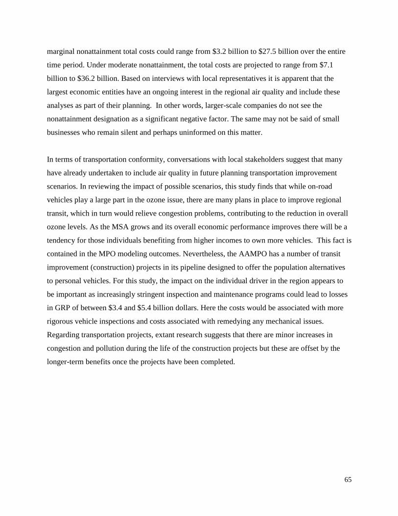
65
marginal nonattainment total costs could range from $3.2 billion to $27.5 billion over the entire
time period. Under moderate nonattainment, the total costs are projected to range from $7.1
billion to $36.2 billion. Based on interviews with local representatives it is apparent that the
largest economic entities have an ongoing interest in the regional air quality and include these
analyses as part of their planning. In other words, larger-scale companies do not see the
nonattainment designation as a significant negative factor. The same may not be said of small
businesses who remain silent and perhaps uninformed on this matter.
In terms of transportation conformity, conversations with local stakeholders suggest that many
have already undertaken to include air quality in future planning transportation improvement
scenarios. In reviewing the impact of possible scenarios, this study finds that while on-road
vehicles play a large part in the ozone issue, there are many plans in place to improve regional
transit, which in turn would relieve congestion problems, contributing to the reduction in overall
ozone levels. As the MSA grows and its overall economic performance improves there will be a
tendency for those individuals benefiting from higher incomes to own more vehicles. This fact is
contained in the MPO modeling outcomes. Nevertheless, the AAMPO has a number of transit
improvement (construction) projects in its pipeline designed to offer the population alternatives
to personal vehicles. For this study, the impact on the individual driver in the region appears to
be important as increasingly stringent inspection and maintenance programs could lead to losses
in GRP of between $3.4 and $5.4 billion dollars. Here the costs would be associated with more
rigorous vehicle inspections and costs associated with remedying any mechanical issues.
Regarding transportation projects, extant research suggests that there are minor increases in
congestion and pollution during the life of the construction projects but these are offset by the
longer-term benefits once the projects have been completed.
66
6. References
Alamo Area Council of Governments (AACOG). 2016. Alamo Ozone Advance Program:
Regional Sustainability Initiatives. San Antonio, TX: AACOG. 76pp.
https://www.epa.gov/sites/production/files/2016-08/documents/update.july_2016.pdf
Alamo Area Metropolitan Planning Organization (AAMPO). 2016a. Transportation Conformity
(Powerpoint Presentation). San Antonio, TX: AAMPO. 11pp.
http://www.alamoareampo.org/AirQuality/conformity-
docs/16.08.22%20AAMPO%20TPB%20Final%20Ver%20Presentation%20Transportation%20C
onformity.pdf (accessed 20 November 2016).
AAMPO. 2016b. Transportation Conformity: Regionally Significant Roadway Definition
(Powerpoint Presentation). San Antonio, TX: AAMPO. 23pp.
http://www.alamoareampo.org/AirQuality/conformity-
docs/Regionally%20Significant%20Roadways%2008%2022%202016.pdf (accessed 20
November 2016).
AAMPO. 2016c. FY 2017 – 2020: Transportation Improvement Program. San Antonio, TX:
AAMPO. 134pp. http://www.alamoareampo.org/Plans/TIP/docs/TIP_2017-2020.pdf (accessed
20 November 2016).
AAMPO. 2015. “Mobility 2040”. Alamo Area Metropolitan Planning Organization
Metropolitan Transportation Plan. San Antonio, TX: AAMPO. 310pp.
http://www.alamoareampo.org/Plans/MTP/docs/Mobility2040/Final%20MTP%20Revised%20M
arch%2010%202015.pdf (accessed 20 November 2016).
Blankenheim, C. 2013. Estimating the Economic Impact of Ozone and Fine Particulate
Nonattainment in the Twin Cities: A Plan B Paper. M.S. Thesis, University of Minnesota.
(April 10, 2013). 63 pp.
http://conservancy.umn.edu/bitstream/handle/11299/150030/Blankenheim_Estimating%20the%2
0Economic%20Impact.pdf;sequence=1 (accessed 31 August 2016).
Capital Area Council of Governments (CAPCOG). 2015. The Potential Costs of an Ozone
Nonattainment Designation to Central Texas. PGA FY14-1, Deliverable 1.3.4, Amendment 1.
Austin, TX: CAPCOG. (September 22, 2015).
City of Wichita (Kansas). 2012. Consequences of Nonattainment Designation for the Wichita
Area. Wichita, KS: Wichita Air Quality Improvement Task Force, Office of Environmental
Initiatives Metropolitan Area Planning Department Wichita. April 2, 2012.
http://www.wichita.gov/Government/News/Supplemental%20Documents/Consequences%20of%
20a%20Nonattainment%20Designation%20042012.pdf (accessed 31 August 2016).
de la Garza, P.E., Anna. Zephyr Environmental Corporation, email correspondence, January 25,
2017.
67
Eastern Research Group, Inc. 2016. Evaluation of the Texas Vehicle Emissions Inspection and
Maintenance Program in the Dallas-Fort Worth and Houston-Galveston-Brazoria Nonattainment
Areas. Prepared for Texas Commission on Environmental Quality. June 30, 2016.
Eastern Research Group, Inc. 2016b. Vehicle Emissions Inspection Program Test Fee Analysis
for AirCheckTexas Program. July 30, 2016. Prepared for: TCEQ Air Quality Division.
Environ International Corporation. 2015. Final Report Potential Emission Control Strategies
Available for Evaluation by the City of San Antonio. Novato, CA: Environ International
Corporation. (March 2015).
https://www.sanantonio.gov/Portals/0/Files/Sustainability/Environ%20Report.pdf. (accessed 31
August 2016).
Environmental Protection Agency (EPA). 2016a. NAAQS Table. Washington, DC: EPA.
https://www.epa.gov/criteria-air-pollutants/naaqs-table (accessed 09 January 2017)
EPA. 2016b. Implementation of the 2015 National Ambient Air Quality Standards for Ozone:
Nonattainment Area Classifications and State Implementation Plan Requirements. Federal
Register Vol. 81, No. 222. November 17, 2016. (81276 – 81317).
https://www.gpo.gov/fdsys/pkg/FR-2016-11-17/pdf/2016-27333.pdf (accessed 11 January 2017)
EPA. 2016c. SIP Status and Information | Criteria Air Pollutants | Nonattainment Area & OTR
SIP Requirements. Washington, DC: EPA,
https://www3.epa.gov/airquality/urbanair/sipstatus/nonattainment.html (accessed 20 September
2016).
EPA. 2016d. SIP Status and Information | Criteria Air Pollutants | Infrastructure SIP
Requirements. Washington, DC: EPA.
https://www3.epa.gov/airquality/urbanair/sipstatus/infrastructure.html (accessed 20 September
2016).
EPA. 2016e. Status of SIP Requirements for Designated Areas | Nonattainment Area & OTR
SIP Requirements | State Implementation Plan Status | Six Common Pollutants | Air & Radiation
| Washington, DC: EPA.
https://www3.epa.gov/airquality/urbanair/sipstatus/reports/tx_elembypoll.html#ozone-
8hr__2008__1404 (accessed 20 September 2016).
EPA. 2016f. New Source Review (NSR) Permitting | Nonattainment NSR Basic Information.
Washington, DC: EPA. https://www.epa.gov/nsr/nonattainment-nsr-basic-information (accessed
22 November 2016).
EPA. 2016g. Implementing Reasonably Available Control Technology Requirements for
Sources Covered by the 2016 Control Techniques Guidelines for the Oil and Natural Gas
Industry. Memo from Anne Marie Wood to Regional Air Division Directors, 1 – 10.
https://www.epa.gov/nsr/nonattainment-nsr-basic-information

68
EPA. 2016h. Required SIP Elements by Nonattainment Classification. Washington, DC: EPA
https://www.epa.gov/ozone-pollution/required-sip-elements-nonattainment-classification
(accessed 06 December 2016).
EPA. 2015a. 40 CFR Part 50, 51, 52, et al., National Ambient Air Quality Standards for Ozone;
Final Rule. Federal Register Vol. 80, No. 206. October 26, 2015. (65291 – 65468)
EPA. 2015b. Clean Air Act Anti-backsliding Requirements and Implications for the Houston
Area. Presentation by Carl Young, U.S. EPA, Region 6 (March 26, 2015). http://www.h-
gac.com/taq/airquality/raqpac/documents/2015/Mar%2026/EPA%20R6%20RAQPAC%20prese
ntation%20for%203-26-2015%20on%20Anti-backsliding.pdf (accessed 15 January 2017).
March 26, 2015EPA. 2014. Regulatory Impact Analysis of the Proposed Revisions to the
National Ambient Air Quality Standards for Ground-Level Ozone. EPA-452/P-14-006.
Washington, DC: EPA. (November 2014). 575 pp.
https://www3.epa.gov/ttnecas1/regdata/RIAs/20141125ria.pdf (accessed 31 August 2016).
EPA. 2012. Transportation Conformity Guidance for 2008 Ozone Nonattainment Areas. EPA-
420-B-12-045. Washington, DC: Transportation and Climate Division Office of Transportation
and Air Quality EPA. 24 pp. July.
http://nepis.epa.gov/Exe/ZyPDF.cgi?Dockey=P100EQWQ.pdf. (accessed 25 October 2016).
EPA. 2006. EPA’s Oversight of the Vehicle Inspection and Maintenance Program Needs
Improvement. Report No. 2007-P-00001. Washington, DC: Office of the Inspector General,
EPA. October 5, 2006. https://www.epa.gov/sites/production/files/2015-
11/documents/20061005-2007-p-00001.pdf (accessed 12 December 2016).
EPA. 1993. 40 CFR Part 6, 51, and 93, Determining Conformity of General Federal Actions to
State or Federal Implementation Plans; Final Rule. Federal Register Vol. 58, No. 228.
November 30, 1993. (63213 – 63259)
Federal Aviation Administration/Environmental Protection Agency (FAA/EPA). 2002. General
Conformity Guidance for Airports: Questions and Answers. Washington, DC: FAA Office of
Airport Planning and Programming, Community and Environmental Needs Division; EPA
Office of Air Quality Planning and Standards, Air Quality Strategies and Standards Division.
September 25, 2002. https://www.epa.gov/sites/production/files/2016-
03/documents/airport_qa.pdf (accessed 20 November 2016).
Federal Highway Administration (FHWA). 2016. Clean Air Act Sanctions. Washington, DC:
FHWA. http://www.fhwa.dot.gov/environment/air_quality/highway_sanctions/index.cfm
(accessed 13 December 2016).
FHWA. 2010. Transportation Conformity: A Basic Guide for State and Local Officials.
FHWA-HEP-11-001. Washington, DC: U.S. Department of Transportation, FHWA.
http://www.fhwa.dot.gov/environment/air_quality/conformity/guide/ (accessed 25 October
2016).

69
Halebic, Maya and Nivin, Steve. 2012. Small Business Study: A Profile of Small Businesses in
the San Antonio Metro Area. February 2012. SABER Institute.
Houston-Galveston Area Council (HGAC). 2016. 2016 Budget and Service Plan. http://www.h-
gac.com/financial/documents/2016-budget-and-service-plan.pdf (accessed 1 February 2017).
IMPLAN. 2015. IMPLAN Data Sources.
http://support.implan.com/index.php?option=com_content&view=article&id=250:250&catid=22
2:222
NERA Economic Consulting. 2015a. Economic Impacts of a 65 ppb National Ambient Air
Quality Standard for Ozone. Prepared for the National Association of Manufacturers. February
2015. 142 pp. http://www.nam.org/Issues/Energy-and-Environment/Ozone/Economic-Impacts-
of-a-65-ppb-NAAQS-for-Ozone-(NERA).pdf (accessed 01 September 2016)
NERA Economic Consulting. 2015b. What Could New Ozone Regulations Cost Texas?
Prepared for the National Association of Manufacturers. http://www.nam.org/Issues/Energy-
and-Environment/Ozone/State-Data/Texas-Ozone-Data-2015.pdf. August 2015. (accessed 31
August 2016)
Office of Management and Budget. 2015. OMB Bulletin No. 15-01: Revised Delineation of
Metropolitan Statistical Areas, Micropolitan Statistical Areas, and Combined Statistical Areas,
and Guidance on Uses of the Delineations of These Areas. July 15, 2015.
https://www.whitehouse.gov/sites/default/files/omb/bulletins/2015/15-01.pdf
PCA. 2015. Ozone NAAQS Concerns. PowerPoint presentation provided by PCA.
San Antonio Business Journal. 2016. 2016-2017 Book of Lists. Business Journal Publications,
Inc. p. 174.
SA Tomorrow. Multimodal Transportation Plan.
http://www.satransportationplan.com/app_pages/view/394 (accessed 30 December 2016).
Small Businesses Administration, Office of Advocacy, Thomas M. Sullivan, letter to EPA
Administrator Stephen Johnson, Small Business Administration, July, 8, 2008, pp. 5–6, at
http://www.uschamber.com/NR/rdonlyres/ews52uzc7sh7u75ygwbmydmu4jnddkqimtlptavoujofl5u
zcwgbtwfj4jp7orw5e7zc7evmcy25nv3aqoxuemk32vb/SBALettertoEPAJuly2008.pdf (January 19,
2010).
Texas Commission on Environmental Quality (TCEQ). 2016a. Agenda Item Request for
Approval of the 2015 Ozone NAAQS Designation Recommendation to the Governor (Docket
No. 2016-0399-SIP). Austin, TX: TCEQ. (Agenda Requested: August 3, 2016).
https://www.tceq.texas.gov/airquality/sip/eighthour.html (accessed 31 August 2016)

70
TCEQ. 2016b. Agenda Item Request for State Implementation Plan Revision Adoption.
(Docket No. 2015-1380-SIP). Agenda Requested: August 3, 2016. (Agenda Requested: July 6,
2016). https://www.tceq.texas.gov/airquality/sip/eighthour.html (accessed 31 August 2016)
TCEQ. 2016c. Texas Counties Exceeding the 2015 Ozone NAAQS Based on Preliminary 2015
Ozone Design Values. Map (February 29, 2016). Austin, TX: TCEQ.
https://www.tceq.texas.gov/airquality/sip/eighthour.html (accessed 31 August 2016).
TCEQ. 2016d. Air NSR Permits: Index of Common Permitted Facilities. Austin, TX: TCEQ.
http://tceq.net/permitting/air/guidance/newsourcereview/ (accessed 9 October 2016)
TCEQ. 2016e. Implementation of the Expedited Permitting Program. TCEQ-(APDG 6258v6,
Revised 09/16). Austin, TX: TCEQ.
https://www.tceq.texas.gov/permitting/air/nav/air_docs_newsource.html (accessed 7 October
2016).
TCEQ. 2016f. Texas Commission on Environmental Quality Fact Sheet - Air Permitting.
Austin, TX: TCEQ. March.
https://www.tceq.texas.gov/assets/public/permitting/air/factsheets/permit_factsheet.pdf (accessed
7 October 2016).
TCEQ. 2016g. Air Quality Successes - Air Permits. Austin, TX: TCEQ. July.
https://www.tceq.texas.gov/airquality/airsuccess/airSuccessPermits (accessed 9 October 2016).
TCEQ. 2016h. Vehicle Emissions Inspections in Texas: Program Overview of the Vehicle
Inspection And Maintenance (I/M) Program In Texas. Austin, TX: TCEQ.
https://tceq.state.tx.us/airquality/mobilesource/vim/overview.html (accessed 12 December 2016).
TCEQ. 2016i. Fact Sheet – Air Permitting. March 2016. Austin, TX: TCEQ.
https://www.tceq.texas.gov/assets/public/permitting/air/factsheets/permit_factsheet.pdf
TCEQ. 2016j. SIP 101. Presentation by to Alamo Area Council of Governments by Dan
Robicheaux (September 12, 2016), Austin, TX: SIP Team, Air Quality Planning Section, Air
Quality Division, TCEQ. http://www.aacog.com/ArchiveCenter/ViewFile/Item/1462 (accessed
11 January 2017).
TCEQ. 2016k. Texas Low Emission Diesel (TxLED) Program. Austin, TX: TCEQ.
https://www.tceq.texas.gov/airquality/mobilesource/txled/cleandiesel.html (accessed 15 January
2017).
TCEQ. 2016l. Gasoline Vapor Recovery (Stages I and II). Austin, TX: TCEQ.
https://www.tceq.texas.gov/airquality/mobilesource/vapor_recovery.html (accessed 15 January
2017).

71
TCEQ. 2016m. Texas Emissions Reduction Program (TERP). January 2016. Austin, TX: TCEQ.
https://www.h-gac.com/taq/airquality/raqpac/documents/2016/2016-01-
28/TERP%20RAQPAC%20012816%204.pdf
TCEQ. 2015a. Consideration of the Adoption of the Dallas-Fort Worth (DFW) Reasonable
Further Progress (RFP) State Implementation Plan (SIP) Revision for the 2008 Eight-Hour
Ozone National Ambient Air Quality Standard (NAAQS). Texas Commission on Environmental
Quality Agenda Item Request for State Implementation Plan Revision Adoption (Docket No.
2014-1249-SIP). Austin, TX: TCEQ. (Agenda Requested: June 3, 2015).
TCEQ. 2015b. Redesignation Substitute Report For The Houston-Galveston-Brazoria 1997
Eight-Hour Ozone Standard Nonattainment Area. Austin, TX: TCEQ.
https://www.tceq.texas.gov/assets/public/implementation/air/sip/hgb/1997ozone_RS_Report/HG
B_RS_1997_8Hr_report.pdf (accessed 13 December 2016).
TCEQ. 2011. Air Permit Reviewer Reference Guide: Air Pollution Control. How to Conduct a
Pollution Control Evaluation (APDG 6110). Austin, TX: TCEQ. 54 pp. .
https://www.tceq.texas.gov/assets/public/permitting/air/Guidance/NewSourceReview/airpoll_gui
dance.pdf (accessed 22 November 2016).
Texas Department of Public Safety (TX DPS). Cost of Inspection.
http://www.dps.texas.gov/RSD/VI/CostOfInsp.htm (accessed 30 December 2017).

Contract (Grant) # 582-16-60180
PGA 582-16-60849-01
Task 5.2
Appendix A
Texas Examples of SIP Requirements for Nonattainment Designation

A-1
Table A.1. Example of SIP Requirements for Nonattainment Designation - Marginal
Texas: Ozone-(8-hr, 2008) / Houston-Galveston-Brazoria
(From EPA, 2016e)
SIP Requirement Deadline Submittal Date Latest Action Date of Latest Action
FR Citation
Click to view
FR notice
Emission Inventory 07/20/2014 07/18/2014 Approval 04/21/2015 80 FR 9204
Emission Statement 07/20/2014 10/27/1992 Approval 10/25/1994 59 FR 44036
Nonattainment NSR rules – Marginal 07/20/2015 11/13/1992 Approval 11/27/1995 60 FR 49781

A-2
Table A.2. Example of SIP Requirements for Nonattainment Designation - Moderate
Texas: Ozone (8-hr, 2008) / Dallas-Fort Worth
(From EPA, 2016e)
SIP Requirement Deadline Submittal
Date Latest Action
Date of Latest
Action
FR
Citation
Click to
view
FR notice
Contingency Measures VOC and NOx 07/20/2015 07/13/2015 Completeness 01/13/2016
Emission Inventory 07/20/2014 07/18/2014 Approval 04/21/2015 80 FR
9204
Emission Statement 07/20/2014 10/27/1992 Approval 10/25/1994 59 FR
44036
I/M Basic 07/20/2015 07/13/2015 Completeness 01/13/2016
Nonattainment NSR rules - Moderate 07/20/2015 11/13/1992 Approval 11/27/1995 60 FR
49781
Ozone Attainment Demonstration 07/20/2015 07/13/2015 Completeness 01/13/2016
RACT Non-CTG VOC for Major Sources 07/20/2014 07/13/2015 Completeness 01/13/2016
RACT NOx for Major Sources 07/20/2014 07/13/2015 Completeness 01/13/2016
RACT VOC CTG Aerospace 07/20/2014 07/13/2015 Completeness 01/13/2016
RACT VOC CTG Auto and Light-Duty Truck Assembly
Coatings (2008) 07/20/2014 07/13/2015 Completeness 01/13/2016
RACT VOC CTG Bulk Gasoline Plants 07/20/2014 07/13/2015 Completeness 01/13/2016
RACT VOC CTG Equipment Leaks from Natural
Gas/Gasoline Processing Plants 07/20/2014 07/13/2015 Completeness 01/13/2016
RACT VOC CTG Factory Surface Coating of Flat Wood
Paneling 07/20/2014 07/13/2015 Completeness 01/13/2016
RACT VOC CTG Fiberglass Boat Manufacturing
Materials (2008) 07/20/2014 07/13/2015 Completeness 01/13/2016
RACT VOC CTG Flat Wood Paneling Coatings (2006) 07/20/2014 07/13/2015 Completeness 01/13/2016
RACT VOC CTG Flexible Packaging Printing Materials
(2006) 07/20/2014 07/13/2015 Completeness 01/13/2016
RACT VOC CTG Fugitive Emissions from Synthetic
Organic Chemical Polymer and Resin Manufacturing
Equipment
07/20/2014 07/13/2015 Completeness 01/13/2016
RACT VOC CTG Graphic Arts - Rotogravure and
Flexography 07/20/2014 07/13/2015 Completeness 01/13/2016
RACT VOC CTG Industrial Cleaning Solvents (2006) 07/20/2014 07/13/2015 Completeness 01/13/2016
RACT VOC CTG Large Appliance Coatings (2007) 07/20/2014 07/13/2015 Completeness 01/13/2016
RACT VOC CTG Large Petroleum Dry Cleaners 07/20/2014 07/13/2015 Completeness 01/13/2016
RACT VOC CTG Leaks from Gasoline Tank Trucks and
Vapor Collection Systems 07/20/2014 07/13/2015 Completeness 01/13/2016
RACT VOC CTG Leaks from Petroleum Refinery
Equipment 07/20/2014 07/13/2015 Completeness 01/13/2016
RACT VOC CTG Lithographic Printing Materials and
Letterpress Printing Materials (2006) 07/20/2014 07/13/2015 Completeness 01/13/2016
RACT VOC CTG Manufacture of High-Density
Polyethylene, Polypropylene, and Polystyrene Resins 07/20/2014 07/13/2015 Completeness 01/13/2016
RACT VOC CTG Manufacture of Pneumatic Rubber
Tires 07/20/2014 07/13/2015 Completeness 01/13/2016

A-3
RACT VOC CTG Manufacture of Synthesized
Pharmaceutical Products 07/20/2014 07/13/2015 Completeness 01/13/2016
RACT VOC CTG Metal Furniture Coatings (2007) 07/20/2014 07/13/2015 Completeness 01/13/2016
RACT VOC CTG Miscellaneous Industrial Adhesives
(2008) 07/20/2014 07/13/2015 Completeness 01/13/2016
RACT VOC CTG Miscellaneous Metal Products Coatings
(2008) 07/20/2014 07/13/2015 Completeness 01/13/2016
RACT VOC CTG Paper, Film, and Foil Coatings (2007) 07/20/2014 07/13/2015 Completeness 01/13/2016
RACT VOC CTG Petroleum Liquid Storage in External
Floating Roof Tanks 07/20/2014 07/13/2015 Completeness 01/13/2016
RACT VOC CTG Plastic Parts Coatings (2008) 07/20/2014 07/13/2015 Completeness 01/13/2016
RACT VOC CTG Refinery Vacuum Producing Systems,
Wastewater Separators, and Process Unit Turnarounds 07/20/2014 07/13/2015 Completeness 01/13/2016
RACT VOC CTG SOCMI Air Oxidation Processes 07/20/2014 07/13/2015 Completeness 01/13/2016
RACT VOC CTG SOCMI Distillation and Reactor
Processes 07/20/2014 07/13/2015 Completeness 01/13/2016
RACT VOC CTG Shipbuilding/repair 07/20/2014 07/13/2015 Completeness 01/13/2016
RACT VOC CTG Solvent Metal Cleaning 07/20/2014 07/13/2015 Completeness 01/13/2016
RACT VOC CTG Stage I Vapor Control Systems -
Gasoline Service Stations 07/20/2014 07/13/2015 Completeness 01/13/2016
RACT VOC CTG Storage of Petroleum Liquids in Fixed
Roof Tanks 07/20/2014 07/13/2015 Completeness 01/13/2016
RACT VOC CTG Surface Coating for Insulation of
Magnet Wire 07/20/2014 07/13/2015 Completeness 01/13/2016
RACT VOC CTG Surface Coating of Automobiles and
Light-Duty Trucks 07/20/2014 07/13/2015 Completeness 01/13/2016
RACT VOC CTG Surface Coating of Cans 07/20/2014 07/13/2015 Completeness 01/13/2016
RACT VOC CTG Surface Coating of Coils 07/20/2014 07/13/2015 Completeness 01/13/2016
RACT VOC CTG Surface Coating of Fabrics 07/20/2014 07/13/2015 Completeness 01/13/2016
RACT VOC CTG Surface Coating of Large Appliances 07/20/2014 07/13/2015 Completeness 01/13/2016
RACT VOC CTG Surface Coating of Metal Furniture 07/20/2014 07/13/2015 Completeness 01/13/2016
RACT VOC CTG Surface Coating of Miscellaneous
Metal Parts and Products 07/20/2014 07/13/2015 Completeness 01/13/2016
RACT VOC CTG Surface Coating of Paper 07/20/2014 07/13/2015 Completeness 01/13/2016
RACT VOC CTG Tank Truck Gasoline Loading
Terminals 07/20/2014 07/13/2015 Completeness 01/13/2016
RACT VOC CTG Use of Cutback Asphalt 07/20/2014 07/13/2015 Completeness 01/13/2016
RACT VOC CTG Wood Furniture 07/20/2014 07/13/2015 Completeness 01/13/2016
RFP VOC and NOx - Moderate 07/20/2015 07/13/2015 Completeness 01/13/2016