potato potential eastern seaboard - university of vermont

Agronomy Journa l • Volume106 , I s sue1 • 2014 43

Biometry, Modeling & Statistics

BiophysicalConstraintstoPotentialProductionCapacityofPotatoacrosstheU.S.EasternSeaboardRegion

JonathanP.Resop,*DavidH.Fleisher,DennisJ.Timlin,andV.R.Reddy

Published in Agron. J. 106:43–56 (2014)doi:10.2134/agronj2013.0277Copyright © 2014 by the American Society of Agronomy, 5585 Guilford Road, Madison, WI 53711. All rights reserved. No part of this periodical may be reproduced or transmitted in any form or by any means, electronic or mechanical, including photocopying, recording, or any information storage and retrieval system, without permission in writing from the publisher.

ABSTRACT� e Eastern Seaboard region (ESR) of the United States is densely populated and depends on imported food. Agricultural systems are vulnerable to uncertainties such as environmental conditions, climate change, and transportation costs. Local populations could bene� t from regional food systems as a way to provide security; however, the potential production capacity of the region would � rst need to be quanti� ed. Potential production capacity for a speci� c crop, potato (Solanum tuberosum L.), was explored in two ways: expansion of the harvested land area and closing the yield gap between observed and potential yield. Potato production was assessed from Maine to Virginia for current land use (land under potato cultivation) and potential land use (other cropland). Simulations were based on two water availability scenarios: limited and nonlimited. A geospatial model implementing the explanatory model SPUDSIM estimated crop production (crop yield, water use, and N uptake) based on spatially variable input data (weather, soil, and management). Potato production was simulated in 35 potato-producing counties and in 346 counties with cropland. Under water-limited conditions, the response surface of production showed greater yield in the northern ESR states (median 28.24 Mg ha–1) than in the southern states (median 15.41 Mg ha–1). Resource requirements (water and N) and biophysical constraints (climate and soil) to production were also evaluated. In general, potato yield was negatively correlated with higher average seasonal temperatures and denser soil pro� les. � e results from this study will be valuable for regional policy planners to assess the capacity of the regional ESR food system.

USDA-ARS, Crop Systems and Global Change Lab., Bldg. 001, Room 342, 10300 Baltimore Ave., Beltsville, MD 20705. Received10 June 2013. *Corresponding author ([email protected]).

Abbreviations: CDL, Cropland Data Layer; ESR, Eastern Seaboard region; MU, modeling unit; NASS, National Agricultural Statistics Service; NL, nonlimited; NLCD, National Land Cover Database; SSURGO, Soil Survey Geographic; WL, water limited.

Foodsystemsplayacriticalrole in the well-being of society and are impacted by many uncertainties, such as the suitability of natural resources (e.g., soil and climate) for plant growth and the fl uctuating energy costs associated with transportation, which lead to concerns over food security. Th is is particularly an issue for densely populated urban areas, such as the U.S. ESR (Maine to Virginia), which represents 23% of the U.S. population (2010 U.S. Census). It is estimated that 12% of the ESR is food insecure, defi ned as households where consumption is reduced due to the lack of resources (Coleman-Jensen et al., 2011). Timmons et al. (2008) estimated the self-suffi ciency of every state by comparing per-capita produc-tion to consumption; weighted by population, the ESR was 24% self-suffi cient, meaning that a majority of food needs to be imported. Individual states ranged from 4% (Massachusetts) to 42% (Delaware). Most other regions in the United States were more self-suffi cient, including highly populated analogs such as California (51%) and Texas (64%). Issues of food security will

only be heightened in future years with uncertainties such as climate change and population growth.

Concerns over food security at the national level have resulted in growing interest for locally produced food. Local food has many potential advantages over larger food systems, such as contributing to local economies, decreasing transportation costs, and creating stronger connections between the local populace and farmers (Feenstra, 1997; Peters et al., 2009; Martinez et al., 2010). Even at the local scale, however, there are ongoing questions and knowledge gaps over issues such as the ability of farms to sustain local populations with the quantity and variety of necessary food and the energy effi ciencies of local-scale food systems (Clancy and Ruhf, 2010; Martinez et al., 2010). As a result, there is increased interest in the study of regional-scale food production systems as a balance between local and global food systems (Stevenson et al., 2011; Peters et al., 2012). While local systems typically encompass 80- to 160-km radii, regional systems are defi ned by boundaries large enough to include multiple states (Clancy and Ruhf, 2010) and thus have the potential to off er greater food production capacity, effi ciency, and security.

Potato production has a long history in the ESR, although the region has been less signifi cant on the national stage in recent years, with only 6.5% of the total U.S. potato production

44 Agronomy Journa l • Volume106, Issue1 • 2014

(2002 Census of Agriculture). There are areas with major potato production, particularly in the northern ESR (such as Aroostook County, Maine). In spite of gains in yield during the last 50 yr, however, overall potato production has decreased (National Agricultural Statistics Service, 2012). The loss of production is the result of a trend of decreasing harvested potato area. The ESR has been losing agricultural land since the early 1900s due to reforestation, industrialization, and a shift of the population to urban areas (Bell, 1989; Foster, 1992). Topsoil erosion resulting from stone removal and continuous cropping has also been a factor in the decline of historically prime farmland (Saini and Grant, 1980; Lal, 1998). The culmination of these dynamics has resulted in the ESR producing fewer potatoes and relying more on importation to satisfy consumption demands. Assuming that 58 kg of potato are consumed per person per year (Economic Research Service, 2012), the annual consumption for the ESR is 4.17 million Mg. Based on the 2002 Census of Agriculture, the total potato production for the ESR was 1.34 million Mg, a self-sufficiency of only 32%. For this reason, potato is a good candidate to study the constraints on potential production for the ESR.

Potential crop yield is defined as the maximum yield of a particular species under optimal soil, water, environment, and management conditions, i.e., no stresses (biotic or abiotic) (Evans and Fischer, 1999; van Ittersum et al., 2003; Cassman et al., 2010). While it is not realistic to achieve full potential, yield simulations can provide theoretical thresholds for the capacity of a region. Yield estimates allow calculation of the difference between theoretical potential yields and actual observed yields—the yield gap (Lobell et al., 2009). Crop yield can be simulated with empirical models or explanatory models. For example, the Erosion–Productivity Impact Calculator (EPIC) was developed for relating soil erosion and productivity but has been used to simulate growth for multiple crops by using a single empirical model (Steiner et al., 1987). This model has been implemented in many studies for predicting crop productivity (Priya and Shibasaki, 2001; Tan and Shibasaki, 2003; Zhang et al., 2010); however, due to the statistical nature of EPIC, it is difficult to make more than generalized predictions of crop yield from the model results. An alternative approach is to use an explanatory model, such as the Decision Support System for Agrotechnology Transfer (DSSAT) models (Jones et al., 2003), Agricultural Production Systems Simulator (APSIM) (McCown et al., 1996), World Food Studies (WOFOST) (van Diepen et al., 1989), and SPUDSIM (Fleisher et al., 2010). Explanatory models are derived based on the physiological processes within the plant and mechanistic depictions of the interface between soil, plant, and atmosphere. As a result, they are better suited to respond to the dynamics related to potential production capacity scenarios, such as land use change and climate change, than are empirical models.

Regional production predictions require the use of geospatial interfaces. The process of linking geospatial data with crop models has been implemented for many applications at various scales (Hartkamp et al., 1999; Hodson and White, 2010). Examples include evaluating climate change effects at the field scale using precision agriculture techniques (Thorp et al., 2008) and at the global scale using coarse-resolution data (Jones and Thornton, 2003). A common strategy is to divide

a region into homogeneous modeling units, simulate crop production independently for each unit, and aggregate the results for analysis (Hansen and Jones, 2000; de Wit et al., 2010). Geospatial crop models have achieved some success in simulating production capacity and yield potential. For example, van Lanen et al. (1992) estimated that 45% of Europe was potentially suitable for wheat (Triticum aestivum L.) production and simulated productivity under water-limited and nonlimited conditions. Lal et al. (1993) simulated the regional productivity of bean (Phaseolus vulgaris L.) for three sites in Puerto Rico and predicted the cultivar and planting date for optimal production at each site. While these studies have demonstrated the effectiveness of quantifying regional productivity with site-specific crop models, they have tended to focus on coarse-resolution data (such as point locations or kilometer-scale rasters). The analysis of regional food systems could be improved by implementing field-scale modeling units to better represent the spatial and temporal heterogeneity of production at the county level (Olesen et al., 2000; Resop et al., 2012).

The purpose of this study was to evaluate the potential production capacity and constraints for potato in the ESR using a geospatial crop model. Potato yield and resource requirements (water use and N uptake) were modeled under water-limited and nonlimited conditions and under current and potential land use scenarios. The sensitivity of the model to variations in climate and soil was used to evaluate constraints. Production of potato was simulated at field-scale modeling units and aggregated to the county level for analysis. Ideally, regional food system analyses should consider multiple crops and socioeconomic factors; however, for the purpose of this study, simulating a single crop was the first step to assessing the biophysical constraints and potential production capacity across the entire region.

METHODS AND MATERIALSGeospatial Crop Model

The process-based crop model SPUDSIM (Fleisher et al., 2010) was implemented for this study to simulate potato production. The model was developed by the USDA-ARS to simulate crop growth at hourly time steps across the length of a season. The mechanistic nature of the model simulates organ-level processes of the plant to estimate crop yield, water use, and N uptake. For simulating root growth and soil water movement, SPUDSIM was combined with the two-dimensional numerical model 2DSOIL (Timlin et al., 1996). Daily weather data were generated with CLIGEN (Nicks et al., 1995) and downscaled to hourly data by SPUDSIM.

Inputs to the crop model can be grouped into three categories: weather (daily values of precipitation, temperature, radiation, relative humidity, and wind speed), soil (initial properties of each horizon such as texture, N, water content, and hydraulic properties), and management (elevation, latitude, longitude, cultivar, irrigation, fertilization, planting depth, planting density, planting date, etc.). Another data type, land use, was not used directly by the crop model, but was instead used to classify the land use and crop cover of each area in the region as a way to determine the locations to simulate (e.g., cropland). For each input category, a data layer was organized for the ESR and georeferenced in ArcGIS version 10.0 (ESRI).

Agronomy Journa l • Volume106, Issue1 • 2014 45

Weather data were generated using the model CLIGEN, a stochastic model that randomly produces daily climate data from monthly statistics based on data observed at National Climatic Data Center weather stations between 1960 and 2009 (Nicks et al., 1995; Meyer et al., 2008). A total of 378 stations was used for the ESR, for a resolution of slightly less than one per county (Fig. 1). Interpolation across the region was performed using Thiessen polygons, which selects the nearest station for each location (Carbone et al., 1996; Liu et al., 2007). For each weather station, 30 independent climate years were generated for the purpose of providing interannual weather variability.

Soil data were derived from the Soil Survey Geographic (SSURGO) database, a high-resolution soil profile database that is available for most areas in the United States at a 1:24,000 scale (Soil Survey Staff, 2012). The data layer divides the ESR into field-scale soil mapping units, which consist of multiple soil components. Each soil component is defined by homogenous soil data. The spatial mapping unit is linked to an extensive database that contains representative values for multiple soil profile properties, such as soil texture, bulk density, and organic matter. Soil hydraulic conductivity and water retention parameters for the van Genuchten equation (van Genuchten, 1980) were determined using the model Rosetta, which estimates using pedotransfer functions (Schaap et al., 2001). Most of the ESR was covered by SSURGO, with the exception of some parts of New Hampshire, New York, and Virginia; however, these areas did not contain any significant amount of cropland.

Due to the lack of high-resolution management data, variables in this category were aggregated at the county scale. For the 13 states in the ESR from Maine to Virginia, there was a total of 435 counties. The centroid latitude and longitude was calculated and the average elevation was derived from the National Elevation Dataset, a 30-m raster (Gesch, 2007). Planting and harvest dates were obtained from the USDA as the average of the most active dates for each state (National Agricultural Statistics Service, 2010) (Table 1).

Other variables were assumed to be constant, such as plant density (4.7 plants m–2), row spacing (84 cm), and initial planting depth (5 cm). The SPUDSIM model was calibrated as described by Fleisher et al. (2010) using 2 yr of growth and yield data for the mid-maturing cultivar Kennebec, which is commonly grown throughout the ESR. The model simulated both water-limited and nonlimited scenarios. It was assumed that crops were grown under unlimited N conditions and were not affected by pests and diseases. National Agricultural Statistics Service (NASS) census data were used for the observed harvested area, yield, and irrigated area at the county level. Area and yield were calculated as the average of the last 4 yr on record (1987, 1992, 1997, and 2002). Irrigation was defined as a percentage of the total harvested area and calculated as the average of the last 2 yr on record (1997 and 2002), except for Rhode Island, for which we used 1992 due to missing data. For counties lacking data, state-level data were used (average of 1990–2009).

The land use data layer was created using a combination of multiple data sources, including Common Land Units (CLUs), the National Land Cover Database (NLCD), and the Cropland Data Layer (CDL). The CLU is a vector polygon data layer developed by the Farm Service Agency that defines agricultural boundaries of contiguous land use and ownership at the field scale (Farm Service Agency, 2012). Land use and land cover were defined by the 2006 NLCD and 2010 CDL, which are both 30-m raster data sets. The NLCD classifies each location into distinct land cover categories, such as developed, forested, pasture, and cropland (Fry et al., 2011). The CDL is similar to the NLCD; however, it also classifies each raster space as a specific crop cover (e.g., potato) for each year (Johnson and Mueller, 2010).

A geospatial crop model interface was developed by combining ArcGIS with SPUDSIM using the scripting language Python version 2.6 (Python Software Foundation). Within ArcGIS, the input data layers (weather, soil, management, and land use) were overlaid to create spatial modeling units (MUs), defined as field-scale polygons with homogeneous properties. The land use and crop cover of

Fig.1.TheNOAAweatherstationsfortheEasternSeaboardregionasanexampleofoneofthegeospatialinputdatalayersusedforanalysis.

Table1.AveragepotatoplantingandharvestdatesintheEasternSeaboardregion(ESR)basedonobserveddata(NationalAgriculturalStatisticsService,2010).

State Plantingdate Harvestdate Seasonlengthd

NorthernESR,fallgrowingseasonMaine 24May 30Sept. 129NewHampshire (nodata,usedMassachusetts)Vermont (nodata,usedMassachusetts)Massachusetts 10May 12Sept. 125RhodeIsland 12May 8Sept. 119Connecticut (nodata,usedMassachusetts)NewYork 5 May 8Sept. 126Pennsylvania 13May 17Sept. 127

SouthernESR,summergrowingseasonNewJersey 11May 25Aug. 106Maryland 20Apr. 31July 102Delaware 21Apr. 7Aug. 108WestVirginia (nodata,usedMaryland)Virginia (nodata,usedMaryland)


each MU were determined by the majority value of the NLCD and CDL, respectively. The MUs were then grouped together based on land use class and unique combinations of the input data used by the crop model (weather, soil, and management). A Python script was used to create a set of unique input combinations for each land use scenario. For each input combination, 30 yr of crop production were simulated to produce outputs of dry tuber mass, water use, and N uptake. Tuber dry mass was converted to a fresh yield area basis (Mg ha–1) using the planting density and assumed moisture content of 80% (Kolbe and Stephan-Beckmann, 1997). Simulations were linked back to the individual MUs, and the field-scale results were aggregated to the county level by averaging across the 30 yr and weighting by the relative area. The Python interface automated the processes of simulation, linkage, and aggregation. For more information about the methodology used in this study, a more detailed description was presented by Resop et al. (2012).

Land Use Availability Scenarios and Water Use Conditions

Potato production was simulated for two land use availability scenarios assuming two water use conditions (Table 2). The land use scenarios were separated into current production areas, defined as agricultural land classified as potato, and potential production areas, defined as all cropland. The purpose of these designations was first to simulate productivity in counties with existing production to compare with observed yield from the NASS and then estimate productivity in all counties where potato could potentially be grown. The land use area for each scenario was determined by overlaying the MUs with the NLCD and CDL to calculate the cover percentage of potato land use and cropland. To reduce the amount of required model runs, counties were selected based on a minimum threshold area. For the current land use scenario, 35 counties were selected with at least 50 ha of potato area based on the 2010 CDL. To adequately represent current potato production, 75% of the available area was simulated, about 9 MUs per county. For the potential land use scenario, 346 counties were selected with at least 100 ha of cropland based on the 2006 NLCD. To control the number of simulations, the top three MUs by area were used for each county (Salazar et al., 2012). Once the available area was determined for each land use scenario, production was simulated for each scenario under both water use conditions.

The first simulation phase used the current land use scenario to establish the baseline production capacity based on where potatoes are currently cultivated. The water-limited (WL) and

nonlimited (NL) results were compared with observed yield and irrigation data from the NASS for validation. Following simulation and validation, the yield gap was evaluated. The yield gap was defined as the difference between actual yield (the average observed NASS yield) and potential (unstressed) yield (the NL theoretical yield) and was expressed as the proportion that observed yield encompassed potential yield. This scenario defined the potential production capacity assuming that only current land is used to its full potential yield.

The second phase simulated WL and NL potato production across an expanded domain using the potential land use scenario to identify trends in yield across the entire ESR. Water use and N uptake were mapped across the region to estimate the expected resource requirements for growing potato in the potential production areas. The resource requirements represent factors affecting yield that are generally under the control of the producer, such as irrigation and fertilization. This scenario defined the potential production capacity assuming that additional land could be used for the potato crop. Following simulation, a sensitivity analysis was performed to evaluate the biophysical constraints (i.e., climate and soil) to production. Constraints represent growth factors that typically cannot be controlled. The sensitivity analysis correlated various climate and soil variables against the estimated yield across all of the simulated MUs in the ESR. The climate variables were precipitation, solar radiation, and maximum and minimum temperatures. Climate variables were averaged across the growing season (except for precipitation, which represented the total rainfall) and across 30 yr of generated weather data. The soil variables were saturated water content, hydraulic conductivity, clay content, and bulk density. Soil variables were averaged along the length of the soil profile, weighted by horizon depth.

RESULTS AND DISCUSSIONLand Use Availability

As a way of validating the land use data layers, the total land in MUs for each land classification as populated by the raster data sets (2006 NLCD and 2010 CDL) was compared with the reported area from the 2007 Census of Agriculture (National Agricultural Statistics Service, 2009). While the mismatched years do not allow a direct comparison, the accuracy of the MUs can be assessed with the closest available data. There are small differences in how cropland is defined by the NASS and the NLCD. The method discussed by Maxwell et al. (2008) for estimating cropland from the NASS (total cropland minus the amount of cropland in pasture and forage) was used to account for these differences. The MUs underestimated the total area in potato cropland by 10% (R2 = 0.98) compared with the NASS surveys (Table 3). For all cropland, the MUs underestimated the total area by 20% (R2 = 0.99). While there is similarity between the land use data sets, the difference in estimating the amount of cropland in the region demonstrates the uncertainty when calculating land use for large areas using different sources of classification data.

There is a large quantity of land that is potentially available for potato production based solely on land use classification (such as cropland, pasture, and grassland). Currently, 41,300 ha are harvested for potato in the ESR (based on the 2007 NASS census) (Table 3). A majority of this takes place in 35 counties

Table2.Descriptionofthelanduseavailabilityscenariosandwateruseconditionsusedforsimulatingtherangeofpotentialproductioncapac-ityfortheEasternSeaboardregion.

Scenario DescriptionLanduseavailabilityscenariosCurrent agriculturallandclassifiedaspotatoPotential allcropland;cultivatedcropsWateruseconditionsWaterlimited cropyieldislimitedbyavailablewater;rainfedagricultureNonlimited cropyieldisnotlimitedbywater;fullyirrigatedagriculture


with at least 50 ha (Fig. 2). The approximately 3.5 million ha of cropland is spread out across the entire ESR, with 346 counties having at least 100 ha. If even a small fraction of the potential area could be converted into potato production, it could result in a dramatic increase in production capacity. For example, if the 311 non-potato-producing counties contributed 50 ha of potato production, it would increase the total harvested area by 38%. The ESR also has a large quantity of uncultivated grassland that could potentially be utilized; however, using these areas for food production could disrupt ecological balances and so it is ideal to first consider increasing production in existing agricultural areas (Lobell et al., 2009).

Before potential land can be used for potato production, other factors need to be considered. First, other limitations, such as rocky soils, steep slopes, and inaccessible fields, may exist. Many of these limitations could be implemented into the geospatial model for future analyses using databases such as SSURGO for soil rockiness, NED for soil slope, and road networks for accessibility. Second, it may not be economically

practical for landowners to convert agricultural land to potato. Ideally, a planner would want to optimize potato production by encouraging growth in areas were potential yield is high and production costs are low. Potato yield is not uniform across the region due to the variability of natural resource constraints.

Current Potato Land Use: Model Validation and Yield Gap

Initial crop model simulations, both water-limited and nonlimited, were performed in areas currently under potato production and compared with observed data from the NASS. The results were first aggregated to the state level to examine regional trends (Table 4). State-level NASS survey data consisted of observed potato yield averaged across 20 yr (1990–2009). The average difference between WL and NL yields was 11.57 Mg ha–1, which represents the gap between the theoretical yield when plants undergo water stress (i.e., rainfed conditions) and the theoretical potential yield assuming no stresses (i.e., a perfectly watered system). This difference was

Table3.Harvestedareaforpotatoandcroplandestimatedbymodel-ingunits(MUs)basedonthe2010CroplandDataLayer(CDL)and2006NationalLandCoverDatabase(NLCD)comparedwiththe2007CensusofAgricultureoftheNationalAgriculturalStatisticsService(NASS).

StatePotato Cropland

NASS CDL NASS NLCD——————————ha——————————

Maine 22,809 25,470 119,171 121,771NewHampshire 32 111 14,013 14,282Vermont 108 47 56,354 67,835Massachusetts 1,059 2,210 31,313 19,213RhodeIsland 219 164 5,244 1,176Connecticut 40 105 28,289 9,118NewYork 7,653 4,928 838,668 810,776Pennsylvania 3,921 1,007 1,102,998 777,180NewJersey 988 726 134,780 143,561Maryland 1,199 498 387,938 392,599Delaware 972 541 165,808 143,349WestVirginia 111 0 54,888 25,453Virginia 2,189 1,450 599,729 317,248Total 41,300 37,257 3,539,193 2,843,561

Fig.2.TotalcroplandareaineachcountyintheEasternSeaboardregionbasedonoverlayingthegeospatialmodelingunitsandthe2006NationalLandCoverDatabase(NLCD).

Table4.Comparisonbetweenobserved(NationalAgriculturalStatisticsService,NASS)andestimatedyield,bothwater-limited(WL)andnonlim-ited(NL),forstatesintheEasternSeaboardregion(ESR)withlandclassifiedascurrentpotatoproductionaswellastheareaofharvestedpotatolandthatwasirrigated.

State

Observed(NASS) Simulated(SPUDSIM)

IrrigatedareaYield WLYield NLYield

Avg. SD Avg. SD Avg. SD%oftotalarea ———————————————————Mgha–1———————————————————

NorthernESR,fallgrowingseasonMaine 12 30.40 2.56 28.81 1.54 38.76 1.29Massachusetts 20 28.89 3.18 26.06 1.38 37.72 0.60RhodeIsland 21 28.08 3.79 27.93 0.81 35.96 0.59NewYork 33 30.97 2.20 27.76 1.49 38.09 0.51Pennsylvania 22 26.98 3.42 27.61 2.19 38.78 0.75SouthernESR,summergrowingseasonNewJersey 74 27.80 2.98 7.62 1.46 25.66 0.47Maryland 67 26.59 6.49 15.11 1.78 25.86 0.73Delaware 70 26.42 4.08 17.45 1.24 27.49 0.68Virginia 53 23.29 3.96 11.21 3.22 25.41 0.60


greater in the southern states than in the northern states. Within the ESR, there existed a clear division between the yield trends in the northern and southern states. Observed potato yields were slightly higher in the north (29.06 Mg ha–1) than in the south (26.02 Mg ha–1). The difference was more profound, however, for the simulated yields. For the WL simulations, the average yield was 27.64 Mg ha–1 in the north compared with 12.85 Mg ha–1 in the south. For the NL simulations, the average yield was 37.86 Mg ha–1 in the north and 26.11 Mg ha–1 in the south.

For a regional-scale scope such as this, there are many potential causes for the differences in yield between the north and south based on the factors affecting production (weather, soil, and management). With respect to weather, potato is known to be a cool-season crop, and the decline in yields for the southern vs. the northern ESR as attributed to climatic differences is probably a result of warmer day- and nighttime air temperatures. Warmer temperatures can result in reduced leaf area, increased senescence rate, a shortened growing

season, and, ultimately, a reduction in biomass including yield (Allen and Scott, 1980). In general, simulations at higher daily temperatures also indicated a higher ratio of respiration to photosynthetic rate (roughly 55% in Virginia and 50% in Maine). In terms of management, two key variables could explain the regional production divide: planting season and irrigation. States in the north are classified by the NASS as having a fall growing season (later planting and harvest dates), while in the south they have a summer growing season (earlier dates and a shorter season) (Table 1). Planting and harvest dates have been shown to affect simulated yield (van Wart et al., 2013) and represent a source of uncertainty that should be explored in future research. Similarly, there is a distinction between irrigation practices in the north and south. Based on the observed area that is irrigated, the averages were 22 and 66% for the north and south, respectively (Table 4). The WL and NL scenarios followed this trend in that in the north the observed yield matched the WL (rainfed) scenario better (relative error 6% for WL and 31% for NL), while in the south

Fig.3.Comparisonbetweencounty-levelobservedyieldintheEasternSeaboardregion(ESR)and(a)water-limitedyieldand(b)nonlimitedyield;(c)thetendencyoferrortoincreaseforwater-limitedyieldastheobservedirrigationincreases;and(d)theadjustedyield,whichtakesirrigationintoaccountandproducedabetterfit.


the observed yield matched the NL (irrigated) scenario better (relative error 50% for WL and 6% for NL).

It is also worth noting that simulations were conducted for the Kennebec cultivar. Kennebec is high yielding and widely adapted to various climates in the United States, including the ESR. The resulting tubers, while predominantly used for chipping, are also suitable for multiple markets including frying and tabletop (Akeley et al., 1948). While this cultivar is moderately resistant to late blight and resistant to tuber net necrosis, it is susceptible to verticillium wilt. There is a large range in the degree to which different potato cultivars possess pest and disease resistance. While we expect the general responses to drought and temperature to be similar among most common cultivars grown in North America, future predictive models that can account for disease prevalence and its associated impact on potato production (not considered in the present case) could potentially reveal an additional source of variation between northern and southern states.

The county-level results had a similar trend as the state level and were compared with observed yields from the NASS. The simulations assuming WL conditions tended to underpredict yield (relative error 22%), while the NL simulations tended to overpredict yield (relative error 31%) (Fig. 3a and 3b). Following the state-level trend between observed irrigation and model accuracy, the WL error increased (Fig. 3c) and NL error decreased (not shown) as irrigation increased. The relative error was 12% for WL yield in the northern counties and 10% for NL yield in the southern counties. These results support the conclusion that regions where management involves more irrigation are better represented by the NL yield, and vice versa. As a result, a composite adjusted yield was calculated by applying the WL yield for the north and NL yield for the south, producing a better fit (relative error 11%) than assuming a single water use condition for the entire region (Fig. 3d). The limitation of regional modeling is that the observed irrigation data are not comprehensive; they are only available at the county level and it is difficult to find data on the amounts of irrigation applied. An alternative approach would be to calculate a weighted yield based on the rainfed area (WL yield) and irrigated area (NL yield), but this approach would also be limited by the observed irrigation data. However, it is important to consider irrigation for regional crop modeling because it is likely to vary and because the model is sensitive to water stress. The need for more irrigation in the south than in the north of the ESR is probably due to many reasons, including seasonal climate conditions, and is explored more below by studying the sensitivity of the model to real-life inputs.

A yield gap analysis was used to evaluate the production capacity for currently cultivated potato areas by quantifying the potential for increasing the average yield. The observed yield was 73% of the potential (nonlimited) yield for the northern (rainfed) counties and 100% for the southern (irrigated) counties. Comparing these numbers with what has been observed in the literature, Lobell et al. (2009) found yield for three crops (corn [Zea mays L.], wheat, and rice [Oryza sativa L.]) to be 50 and 80% of the potential yield for rainfed and irrigated systems, respectively, but noted that yield gap estimates are highly variable. The results for the

southern ESR suggest that actual yield is near the theoretical maximum. Achieving 100% of potential yield in the south is unlikely (considering that the observed irrigated area is not 100%) and realistically the potential for growth should still exist. The underestimation of potential yield is probably due to modeling assumptions and the uncertainty in management factors such as planting date, growing season length, and cultivar. The analysis would also benefit from more observed data on irrigated area and yield; however, census data on potato are sparse. Between the two subregions, there is greater yield potential in the north. Potential yield could be realized by adjusting management practices such as applying irrigation to this historically rainfed region. In the south, if the potential yield gap has truly been eliminated, then attempts to increase local production should focus more on land availability and optimizing the efficiency of resources such as irrigation and fertilization.

Based on the current land use scenario, a few initial conclusions can be made. Assuming WL or NL conditions alone does not adequately represent production for the entire ESR. A better estimate of yield can be generated by considering the observed irrigation practices for the region. The adjusted yield discussed here is a simple example that utilizes both water use scenarios and results in a better fit between observed and estimated yield. Errors observed at the county level are probably due to temporal (climate) and spatial (soil) variability. When estimating regional-scale crop productivity, it is clear that management factors such as planting season and irrigation play an important role in accurate predictions, as emphasized by the differences between northern and southern states as well as between WL and NL model conditions.

Potential Potato Land Use: Resource Requirements and Production Constraints

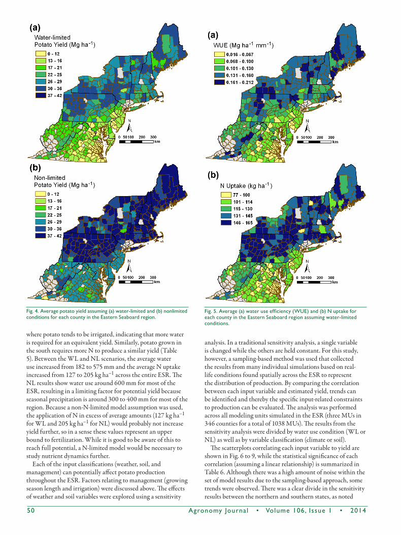
The spatial pattern for the potential land use scenario follows the same trend as the current land use scenario, with yield increasing from south to north (Fig. 4). The median WL yield across the south and north was 15.41 and 28.24 Mg ha–1, respectively, while NL yield was 26.20 and 37.63 Mg ha–1, respectively. The average difference between WL and NL yield was 9.83 Mg ha–1, although it varied among counties (standard deviation 4.63 Mg ha–1). Based on NL yield, the highest productivity was in northwestern Pennsylvania and Maine, where yield was generally >39 Mg ha–1. Assuming no other considerations, these areas represent the greatest potential for production. States in the southern ESR were generally outperformed by the northern states; however, West Virginia stands out because it is not currently a significant potato-producing state in the region. Among the southern states, West Virginia showed the greatest potential for potato production, both for WL and NL yield. With most current potato production occurring in the north, exploring the expansion of potato production into West Virginia could offer high-yielding local production for the southern ESR.

Along with potato yield, plant resource requirements were also estimated under WL and NL conditions. Water use and N uptake followed a similar north–south regional trend as yield, decreasing as yield decreased (Fig. 5). Water use efficiency (crop yield/water use), however, was much lower in the south,


where potato tends to be irrigated, indicating that more water is required for an equivalent yield. Similarly, potato grown in the south requires more N to produce a similar yield (Table 5). Between the WL and NL scenarios, the average water use increased from 182 to 575 mm and the average N uptake increased from 127 to 205 kg ha–1 across the entire ESR. The NL results show water use around 600 mm for most of the ESR, resulting in a limiting factor for potential yield because seasonal precipitation is around 300 to 400 mm for most of the region. Because a non-N-limited model assumption was used, the application of N in excess of average amounts (127 kg ha–1 for WL and 205 kg ha–1 for NL) would probably not increase yield further, so in a sense these values represent an upper bound to fertilization. While it is good to be aware of this to reach full potential, a N-limited model would be necessary to study nutrient dynamics further.

Each of the input classifications (weather, soil, and management) can potentially affect potato production throughout the ESR. Factors relating to management (growing season length and irrigation) were discussed above. The effects of weather and soil variables were explored using a sensitivity

analysis. In a traditional sensitivity analysis, a single variable is changed while the others are held constant. For this study, however, a sampling-based method was used that collected the results from many individual simulations based on real-life conditions found spatially across the ESR to represent the distribution of production. By comparing the correlation between each input variable and estimated yield, trends can be identified and thereby the specific input-related constraints to production can be evaluated. The analysis was performed across all modeling units simulated in the ESR (three MUs in 346 counties for a total of 1038 MUs). The results from the sensitivity analysis were divided by water use condition (WL or NL) as well as by variable classification (climate or soil).

The scatterplots correlating each input variable to yield are shown in Fig. 6 to 9, while the statistical significance of each correlation (assuming a linear relationship) is summarized in Table 6. Although there was a high amount of noise within the set of model results due to the sampling-based approach, some trends were observed. There was a clear divide in the sensitivity results between the northern and southern states, as noted

Fig.4.Averagepotatoyieldassuming(a)water-limitedand(b)nonlimitedconditionsforeachcountyintheEasternSeaboardregion.

Fig.5.Average(a)wateruseefficiency(WUE)and(b)NuptakeforeachcountyintheEasternSeaboardregionassumingwater-limitedconditions.


above. This clustering effect was clearest in the WL radiation data (Fig. 6b). The expected trend was for yield to be positively related to radiation, which was seen in the slight positive trend across each subregion (north and south) individually. Even though the south had higher overall radiation levels than the north, however, it produced smaller yields. This break was also observed in the other scatterplots and suggests that there are other variables, such as management practices (photoperiod, growing season, irrigation, cultivar, etc.) that had a strong regional effect on the estimated yield.

Most of the climate variables had a significant correlation with WL yield. Among all of the variables, temperature by far

had the most influence based on a high negative correlation in both the northern and southern ESR (Fig. 6). As the average seasonal temperature increased, the average yield decreased. For example, the cooler areas of the south, such as West Virginia, generally produced greater yields than the rest of the south. Because seasonal temperature is outside of the control of potato producers, it presents a major constraint to local production. With the effects of future climate change expected to increase global temperatures, this constraint should be evaluated further through additional model simulations to determine the uncertainty in future production. While temperature was a significant factor throughout the ESR, precipitation showed

Table5.Simulatedyieldandresourcerequirements,assumingwater-limited(WL)andnonlimited(NL)conditions,acrossallcountiesintheEasternSeaboardregion(ESR)withpotentialland(i.e.,cropland).

StatisticYield WaterUse NUptake

WL NL WL NL WL NL——————Mgha–1 —————— —————— mm —————— ——————kgha–1 ——————

NorthernESR,fallgrowingseason5thpercentile 19.63 27.03 165 364 115 174Median 28.24 37.63 203 586 147 22195thpercentile 32.75 40.50 228 779 161 229SouthernESR,summergrowingseason5thpercentile 7.06 21.58 136 403 88 177Median 15.41 26.20 165 570 110 19695thpercentile 22.07 29.34 179 690 130 205

Fig.6.Correlationsbetweenaverageweatherconditionsandwater-limitedpotatoyieldintheEasternSeaboardregion(ESR)for(a)precipitation,(b)radiation,(c)maximumtemperature,and(d)minimumtemperature.


no correlation with WL yield in the north and a positive correlation in the south. This pattern could be explained by the observations about irrigation made above. In the north, where the potato crop is predominantly rainfed, there was little plant water stress and so precipitation was not a limiting constraint. In the south, however, the potato crop tends to require irrigation and thus is more likely to experience water stress when relying on rainfed (WL) conditions. For the NL water scenario, the

weather variables were less significant across the board (Fig. 7). This suggests that when water is not a limiting factor, climate conditions play a less dominant role in affecting potato yield.

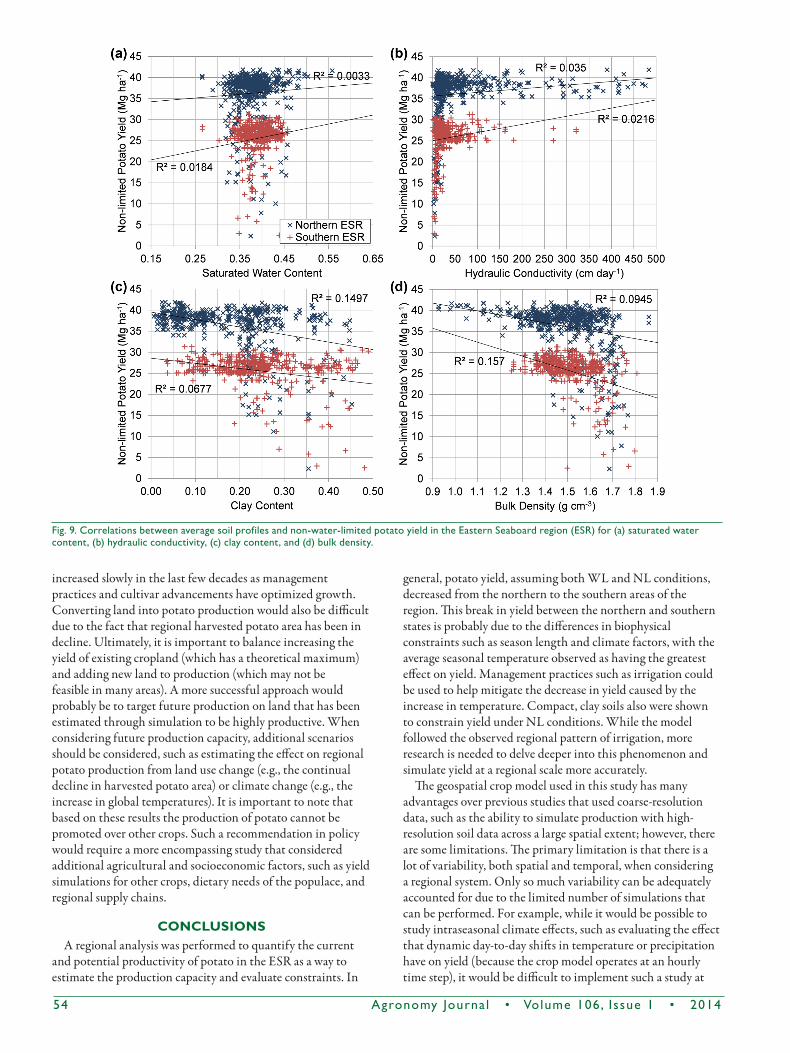
The soil variables did not show a strong correlation with WL yield (Fig. 8). The correlations were much smaller than those of the climate variables, suggesting a dominance of climate factors under WL conditions. For the NL condition, however, the soil variables (except for saturated water content) showed a more

Fig.7.Correlationsbetweenaverageweatherconditionsandnon-water-limitedpotatoyieldintheEasternSeaboardregion(ESR)for(a)precipitation,(b)radiation,(c)maximumtemperature,and(d)minimumtemperature.

Table6.The90%confidenceinterval(CI)andsensitivityanalysisforeachvariable,representedbythecorrelationcoefficient,r,exploringtheeffectofclimateandsoilvariabilityonpotatoyieldintheEasternSeaboardregion(ESR)underbothwater-limited(WL)andnonlimited(NL)conditions.

Variable

NorthernESR SouthernESR

90%CIr

90%CIr

WL NL WL NLClimate Precipitation,mm 302–443 0.08 0.05 270–402 0.19*** 0.05 Radiation,MJm–2d–1 18–21 0.11* –0.06 20–23 0.14** –0.12**

Max.temperature,°C 23–28 –0.55*** –0.20*** 24–29 –0.72*** –0.22***

Min.temperature,°C 10–15 –0.69*** –0.18*** 11–16 –0.85*** –0.19***

Soil Saturatedwatercontent 0.33–0.45 –0.02 0.06 0.34–0.44 0.06 0.14** Hydraulicconductivity,cmd–1 10–350 0.04 0.19*** 10–85 –0.08 0.15*** Claycontent 0.03–0.37 –0.16*** –0.39*** 0.09–0.42 0.10* –0.26*** Bulkdensity,gcm–3 1.18–1.70 –0.03 –0.31*** 1.36–1.69 –0.17*** –0.40****Theslopeforlinearregressionissignificantata=0.05.**Theslopeforlinearregressionissignificantata=0.01.***Theslopeforlinearregressionissignificantata=0.001.


significant correlation with yield (Fig. 9). In essence, the soil variables became more significant than the climate variables when water was no longer a limiting factor. In particular among the soil profile variables, potato yield was constrained when the hydraulic conductivity was <25 cm d–1. This was also evidenced by lower yields when the soil composition was denser, with a higher clay content. While the results show that it was still possible to achieve high potato yields under these conditions (low hydraulic conductivity, denser soil, and higher clay content), this information does help regional planners in determining areas in the ESR where yield is more constrained by the natural environment by avoiding land where soil profiles indicate poor drainage.

Current vs. Potential Production Capacity

The geospatial simulations performed in this study present a way of evaluating the production capacity for potato in the ESR. As discussed above, overall potato production has been on the decline for decades. If one is interested in increasing the amount of local production within the ESR, what is the potential production capacity under various scenarios? As an example, we explored two scenarios: (i) increasing production by increasing actual yield to potential yield (reduce the yield gap); and (ii) increasing production by increasing the harvested potato area and expanding into non-potato-producing counties. Using the current land use scenario as a baseline to

compare simulations, based on the 2010 CDL potato area and the WL yield for the north and NL yield for the south, the current production capacity for the ESR is 1.01 million Mg. As a comparison, the 2002 NASS census observed total production of 1.34 million Mg, which is probably higher due to the decline in harvested potato area during the last decade. The first potential production scenario considered was increasing the yield in current land use areas by eliminating the yield gap and assuming potential (NL) yield in all areas. Under this scenario, the total regional production capacity was estimated to be 1.34 million Mg, an increase of 33% over the baseline value. A majority of new production occurred in the northern ESR, where the yield gap was greater. The second potential scenario assumed an increase in the total land use area by adding 50 ha of production to each county, converting existing cropland to potato. It was assumed that yields followed current patterns using the composite adjusted yield discussed above (WL yield was used in the north and NL yield in the south). Under this scenario, total potato production in the ESR was estimated to be 1.43 million Mg, an increase of 41% over the baseline value. In both cases, the potential production capacity was increased to levels similar to those observed in 2002, regaining production that was lost due to the loss of historic potato land.

Both scenarios discussed here are within the realm of possibility but have limitations. Eliminating the yield gap would be difficult due to the fact that actual yields have

Fig.8.Correlationsbetweenaveragesoilprofilesandwater-limitedpotatoyieldintheEasternSeaboardregion(ESR)for(a)saturatedwatercontent,(b)hydraulicconductivity,(c)claycontent,and(d)bulkdensity.


increased slowly in the last few decades as management practices and cultivar advancements have optimized growth. Converting land into potato production would also be difficult due to the fact that regional harvested potato area has been in decline. Ultimately, it is important to balance increasing the yield of existing cropland (which has a theoretical maximum) and adding new land to production (which may not be feasible in many areas). A more successful approach would probably be to target future production on land that has been estimated through simulation to be highly productive. When considering future production capacity, additional scenarios should be considered, such as estimating the effect on regional potato production from land use change (e.g., the continual decline in harvested potato area) or climate change (e.g., the increase in global temperatures). It is important to note that based on these results the production of potato cannot be promoted over other crops. Such a recommendation in policy would require a more encompassing study that considered additional agricultural and socioeconomic factors, such as yield simulations for other crops, dietary needs of the populace, and regional supply chains.

CONCLUSIONSA regional analysis was performed to quantify the current

and potential productivity of potato in the ESR as a way to estimate the production capacity and evaluate constraints. In

general, potato yield, assuming both WL and NL conditions, decreased from the northern to the southern areas of the region. This break in yield between the northern and southern states is probably due to the differences in biophysical constraints such as season length and climate factors, with the average seasonal temperature observed as having the greatest effect on yield. Management practices such as irrigation could be used to help mitigate the decrease in yield caused by the increase in temperature. Compact, clay soils also were shown to constrain yield under NL conditions. While the model followed the observed regional pattern of irrigation, more research is needed to delve deeper into this phenomenon and simulate yield at a regional scale more accurately.

The geospatial crop model used in this study has many advantages over previous studies that used coarse-resolution data, such as the ability to simulate production with high-resolution soil data across a large spatial extent; however, there are some limitations. The primary limitation is that there is a lot of variability, both spatial and temporal, when considering a regional system. Only so much variability can be adequately accounted for due to the limited number of simulations that can be performed. For example, while it would be possible to study intraseasonal climate effects, such as evaluating the effect that dynamic day-to-day shifts in temperature or precipitation have on yield (because the crop model operates at an hourly time step), it would be difficult to implement such a study at

Fig.9.Correlationsbetweenaveragesoilprofilesandnon-water-limitedpotatoyieldintheEasternSeaboardregion(ESR)for(a)saturatedwatercontent,(b)hydraulicconductivity,(c)claycontent,and(d)bulkdensity.


the regional scale. As another example, the exploratory portion of this research, which used three modeling units per county, was necessary to limit the number of simulations. A more detailed analysis can be performed by doing a coarse analysis like this and then identifying areas for higher resolution simulation. Performing more simulations per county would allow the range of potential yield within each county to be quantified for both productive and marginal land.

The research performed in this study is only the first step in evaluating the potential production capacity of the ESR. Other steps should be taken to further this research and provide regional planners with additional information to optimize food production under multiple uncertainties. For example, additional crops should be included in the analysis as a way to develop a composite yield index. While this study was limited to potato as a way to represent the overall potential productivity, it does not address the fact that certain crops grow better in some areas than others. Such a yield index could be used when performing cost analyses to optimize the regional production of food in a way that lowers transportation costs and increases profit to local farmers. Also, additional sensitivity analyses are needed to quantify the effect of management factors, such as planting date and irrigation, on crop yield. Finally, it is also important to consider the effects of future climate change on regional production in order to determine which areas are most at risk and to figure out how to mitigate any adverse effects.

ACKNOWLEDGEMENTS

This research was supported by the USDA-ARS Headquarters Postdoctoral Research Associate Program and the USDA-NIFA AFRI Grant no. 2011-68004-30057: Enhancing Food Security of Underserved Populations in the Northeast through Sustainable Regional Food Systems. Mention of a trademark or proprietary product does not constitute a guarantee or warranty of the product by the USDA and does not imply the exclusion of other available products. The USDA is an equal opportunity provider and employer.

REFERENCES

Akeley, R.V., F.J. Stevenson, and E.S. Schultz. 1948. Kennebec: A new potato variety resistant to late blight, mild mosaic, and net necrosis. Am. Potato J. 25:351–361. doi:10.1007/BF02883336

Allen, E.J., and R.K. Scott. 1980. An analysis of growth of the potato crop. J. Agric. Sci. 94:583–606. doi:10.1017/S0021859600028598

Bell, M.M. 1989. Did New England go downhill? Geogr. Rev. 79:450–466. doi:10.2307/215118

Carbone, G.J., S. Narurnalan, and M. King. 1996. Application of remote sensing and GIS technologies with physiological crop models. Photogramm. Eng. Remote Sens. 62:171–179.

Cassman, K.G., P. Grassini, and J. van Wart. 2010. Crop yield potential, yield trends, and global food security in a changing climate. In: C. Rosenzweig and D. Hillel, editors, Handbook of climate change and agroecosystems. Imperial College Press, London. p. 37–51.

Clancy, K., and K. Ruhf. 2010. Is local enough? Some arguments for regional food systems. Choices 25(1).

Coleman-Jensen, A., M. Nord, M. Andrews, and S. Carlson. 2011. Household food security in the United States in 2010. USDA Econ. Res. Serv., Washington, DC.

de Wit, A., B. Baruth, H. Boogaard, K. van Diepen, D. van Kraalingen, F. Micale, et al. 2010. Using ERA-INTERIM for regional crop yield forecasting in Europe. Clim. Res. 44:41–53. doi:10.3354/cr00872

Economic Research Service. 2012. Vegetables and pulses: Potatoes. USDA Econ. Res. Serv., Washington, DC.

Evans, L.T., and R.A. Fischer. 1999. Yield potential: Its definition, measurement, and significance. Crop Sci. 39:1544–1551. doi:10.2135/cropsci1999.3961544x

Farm Service Agency. 2012. Common Land Unit data. USDA Farm Serv. Agency, Washington, DC.

Feenstra, G.W. 1997. Local food systems and sustainable communities. Am. J. Altern. Agric. 12:28–36. doi:10.1017/S0889189300007165

Fleisher, D.H., D.J. Timlin, Y. Yang, and V.R. Reddy. 2010. Simulation of potato gas exchange rates using SPUDSIM. Agric. For. Meteorol. 150:432–442. doi:10.1016/j.agrformet.2010.01.005

Foster, D.R. 1992. Land-use history (1730–1990) and vegetation dynamics in central New England, USA. J. Ecol. 80:753–771. doi:10.2307/2260864

Fry, J., G. Xian, S. Jin, J. Dewitz, C. Homer, L. Yang, et al. 2011. Completion of the 2006 National Land Cover Database for the conterminous United States. Photogramm. Eng. Remote Sens. 77:858–864.

Gesch, D.B. 2007. The National Elevation Dataset. In: D. Maune, editor, Digital elevation model technologies and applications: The DEM user’s manual. 2nd ed. Am. Soc. Photogramm. Remote Sens., Bethesda, MD. p. 99–118.

Hansen, J.W., and J.W. Jones. 2000. Scaling-up crop models for climate variability applications. Agric. Syst. 65:43–72. doi:10.1016/S0308-521X(00)00025-1

Hartkamp, A.D., J.W. White, and G. Hoogenboom. 1999. Interfacing geographic information systems with agronomic modeling: A review. Agron. J. 91:761–772. doi:10.2134/agronj1999.915761x

Hodson, D., and J.W. White. 2010. GIS and crop simulation modelling applications in climate change research. In: M.P. Reynolds, editor, Climate change and crop production. CAB Int., Wallingford, UK. p. 245–262.

Johnson, D.M., and R. Mueller. 2010. The 2009 cropland data layer. Photogramm. Eng. Remote Sens. 76:1201–1205.

Jones, J.W., G. Hoogenboom, C.H. Porter, K.J. Boote, W.D. Batchelor, L.A. Hunt, et al. 2003. The DSSAT cropping system model. Eur. J. Agron. 18:235–265. doi:10.1016/S1161-0301(02)00107-7

Jones, P.G., and P.K. Thornton. 2003. The potential impacts of climate change on maize production in Africa and Latin America in 2055. Global Environ. Change 13:51–59. doi:10.1016/S0959-3780(02)00090-0

Kolbe, H., and S. Stephan-Beckmann. 1997. Development, growth and chemical composition of the potato crop (Solanum tuberosum L.): II. Tuber and whole plant. Potato Res. 40:135–153. doi:10.1007/BF02358240

Lal, H., G. Hoogenboom, J.-P. Calixte, J.W. Jones, and F.H. Beinroth. 1993. Using crop simulation models and GIS for regional productivity analysis. Trans. ASAE 36:175–184.

Lal, R. 1998. Soil erosion impact on agronomic productivity and environment quality. Crit. Rev. Plant Sci. 17:319–464. doi:10.1080/07352689891304249

Liu, J., J.R. Williams, A.J.B. Zehnder, and H. Yang. 2007. GEPIC: Modelling wheat yield and crop water productivity with high resolution on a global scale. Agric. Syst. 94:478–493. doi:10.1016/j.agsy.2006.11.019

Lobell, D.B., K.G. Cassman, and C.B. Field. 2009. Crop yield gaps: Their importance, magnitudes, and causes. Annu. Rev. Environ. Resour. 34:179–204. doi:10.1146/annurev.environ.041008.093740

Martinez, S., M. Hand, M. da Pra, S. Pollack, K. Ralston, T. Smith, et al. 2010. Local food systems: Concepts, impacts, and issues. USDA Econ. Res. Serv., Washington, DC.

Maxwell, S.K., E.C. Wood, and A. Janus. 2008. Comparison of the USGS 2001 NLCD to the 2002 USDA Census of Agriculture for the Upper Midwest United States. Agric. Ecosyst. Environ. 127:141–145. doi:10.1016/j.agee.2008.03.012

McCown, R.L., G.L. Hammer, J.N.G. Hargreaves, D.P. Holzworth, and D.M. Freebairn. 1996. APSIM: A novel software system for model development, model testing and simulation in agricultural systems research. Agric. Syst. 50:255–271. doi:10.1016/0308-521X(94)00055-V

Meyer, C.R., C.S. Renschler, and R.C. Vining. 2008. Implementing quality control on a random number stream to improve a stochastic weather generator. Hydrol. Processes 22:1069–1079. doi:10.1002/hyp.6668

National Agricultural Statistics Service. 2009. 2007 Census of agriculture. NASS, Washington, DC.


National Agricultural Statistics Service. 2010. Usual planting and harvesting dates for U.S. field crops. NASS, Washington, DC.

National Agricultural Statistics Service. 2012. Agricultural surveys. NASS, Washington, DC.

Nicks, A.D., L.J. Lane, and G.A. Gander. 1995. Weather generator. In: D.C. Flanagan and M.A. Nearing, editors, USDA-Water Erosion Prediction Project: Hillslope profile and watershed model documentation. Natl. Soil Erosion Res. Lab., West Lafayette, IN. p. 2.1–2.22.

Olesen, J.E., P.K. Bøcher, and T. Jensen. 2000. Comparison of scales of climate and soil data for aggregating simulated yields of winter wheat in Denmark. Agric. Ecosyst. Environ. 82:213–228. doi:10.1016/S0167-8809(00)00227-9

Peters, C.J., N.L. Bills, A.J. Lembo, J.L. Wilkins, and G.W. Fick. 2012. Mapping potential foodsheds in New York state by food group: An approach for prioritizing which foods to grow locally. Renew. Agric. Food Syst. 27:125–137. doi:10.1017/S1742170511000196

Peters, C.J., N.L. Bills, J.L. Wilkins, and G.W. Fick. 2009. Foodshed analysis and its relevance to sustainability. Renew. Agric. Food Syst. 24:1–7. doi:10.1017/S1742170508002433

Priya, S., and R. Shibasaki. 2001. National spatial crop yield simulation using GIS-based crop production model. Ecol. Modell. 136:113–129. doi:10.1016/S0304-3800(00)00364-1

Resop, J.P., D.H. Fleisher, Q. Wang, D.J. Timlin, and V.R. Reddy. 2012. Combining explanatory crop models with geospatial data for regional analyses of crop yield using field-scale modeling units. Comput. Electron. Agric. 89:51–61. doi:10.1016/j.compag.2012.08.001

Saini, G.R., and W.J. Grant. 1980. Long-term effects of intensive cultivation on soil quality in the potato-growing areas of New Brunswick (Canada) and Maine (USA). Can. J. Soil Sci. 60:421–428. doi:10.4141/cjss80-047

Salazar, M.R., J.E. Hook, A.G. Garcia, J.O. Paz, B. Chaves, and G. Hoogenboom. 2012. Estimating irrigation water use for maize in the southeastern USA: A modeling approach. Agric. Water Manage. 107:104–111. doi:10.1016/j.agwat.2012.01.015

Schaap, M.G., F.J. Leij, and M.Th. van Genuchten. 2001. Rosetta: A computer program for estimating soil hydraulic parameters with hierarchical pedotransfer functions. J. Hydrol. 251:163–176. doi:10.1016/S0022-1694(01)00466-8

Soil Survey Staff. 2012. Soil Survey Geographic (SSURGO) database. Natl. Soil Surv. Ctr., Lincoln, NE.

Steiner, J.L., J.R. Williams, and O.R. Jones. 1987. Evaluation of the EPIC simulation model using a dryland wheat–sorghum–fallow crop rotation. Agron. J. 79:732–738. doi:10.2134/agronj1987.00021962007900040030x

Stevenson, G.W., K. Clancy, R. King, L. Lev, M. Ostrom, and S. Smith. 2011. Midscale food value chains: An introduction. J. Agric. Food Syst. Community Dev. 1(4):27–34. doi:10.5304/jafscd.2011.014.007

Tan, G., and R. Shibasaki. 2003. Global estimation of crop productivity and the impacts of global warming by GIS and EPIC integration. Ecol. Modell. 168:357–370. doi:10.1016/S0304-3800(03)00146-7

Thorp, K.R., K.C. DeJonge, A.L. Kaleita, W.D. Batchelor, and J.O. Paz. 2008. Methodology for the use of DSSAT models for precision agriculture decision support. Comput. Electron. Agric. 64:276–285. doi:10.1016/j.compag.2008.05.022

Timlin, D.J., Y.A. Pachepsky, and B. Acock. 1996. A design for a modular, generic soil simulator to interface with plant models. Agron. J. 88:162–169. doi:10.2134/agronj1996.00021962008800020008x

Timmons, D., Q. Wang, and D. Lass. 2008. Local foods: Estimating capacity. J. Ext. 46 (October).

van Diepen, C.A., J. Wolf, H. van Keulen, and C. Rappoldt. 1989. WOFOST: A simulation model of crop production. Soil Use Manage. 5:16–24. doi:10.1111/j.1475-2743.1989.tb00755.x

van Genuchten, M.Th. 1980. A closed-form equation for predicting the hydraulic conductivity of unsaturated soils. Soil Sci. Soc. Am. J. 44:892–898. doi:10.2136/sssaj1980.03615995004400050002x

van Ittersum, M.K., P.A. Leffelaar, H. van Keulen, M.J. Kropff, L. Bastiaans, and J. Goudriaan. 2003. On approaches and applications of the Wageningen crop models. Eur. J. Agron. 18:201–234. doi:10.1016/S1161-0301(02)00106-5

van Lanen, H.A.J., C.A. van Diepen, G.J. Reinds, G.H.J. de Koning, J.D. Bulens, and A.K. Bregt. 1992. Physical land evaluation methods and GIS to explore the crop growth potential and its effects within the European communities. Agric. Syst. 39:307–328. doi:10.1016/0308-521X(92)90102-T

van Wart, J., K.C. Kersebaum, S. Peng, M. Milner, and K.G. Cassman. 2013. Estimating crop yield potential at regional to national scales. Field Crops Res. 143:34–43. doi:10.1016/j.fcr.2012.11.018

Zhang, X., R.C. Izaurralde, D. Manowitz, T.O. West, W.M. Post, A.M. Thomson, et al. 2010. An integrative modeling framework to evaluate the productivity and sustainability of biofuel crop production systems. GCB Bioenergy 2:258–277. doi:10.1111/j.1757-1707.2010.01046.x

potato potential eastern seaboard - university of vermont

Documents