post-tensioned bridge girder anchorage zone enhancement with
TRANSCRIPT
Post-Tensioned Bridge Girder Anchorage Zone
Enhancement with Fiber Reinforced Concrete (FRC)
Final Report
Submitted to
The Florida Department of Transportation (FDOT Contract No. BDB14)
By
Kamal Tawfiq, Ph.D., P.E. Brenda Robinson, Ph.D., P.E., C.G.C.
April 29, 2008

2
DISCLAIMER
The opinions, findings and conclusions expressed in this publication are those of the authors and
do not necessarily reflects those of the State of Florida Department of Transportation
3

4

5
Technical Report Documentation Page 1- Report 2- Government Accession No. 3- Recipients Catalog No.
5- Report Date June 2, 2008
4- Title and Subtitle Post-Tensioned Bridge Girder Anchorage Zone Enhancement with Fiber Reinforced Concrete (FRC)
6- Performing Organization Code
7- Author’s Kamal Tawfiq, and Brenda Robinson
8- Performing organization Report No.
10- Work Unit (TRAIS)
9- Performing Organization Name and Address Florida A & M University Department of Civil and Environmental Engineering FAMU-FSU College of Engineering 2525 Pottsdamer Street Tallahassee, Florida 32312
11-Contract or Grant No BDB14
13 Type of Contract and Period Covered Draft Final (August 2004-March 2008)
12- Sponsoring Agency Name and Address Florida Department of Transportation 605 Suwannee Street Tallahassee, FL 32399-0450
14 Sponsoring Agency Code
15. Supplementary Notes Prepared in cooperation with the U.S. Department of Transportation 16. Abstract The main objective of this research was to investigate the use of steel fiber reinforced concrete (SFRC) in post-tensioning (PT) anchorage zones of bridge girders. The purpose of using SFRC is to enhance the overall performance and to reduce the amount of steel rebar required in the anchorage zone. Reducing steel congestion in post-tensioning anchorage zones can improve the constructability of post-tensioned bridge elements. It was the intent of this investigation of the post-tensioning anchorage zone to consider both the behavior of the local zone and the general zone when steel fiber reinforced concrete is used. To achieve the objectives of this study, both experimental and analytical investigations were conducted aiming at reducing the amount of mild steel reinforcement required by the AASHTO code at the anchorage zone. The experimental part of the study involved laboratory testing of twenty-seven (27) samples representing typical anchorage zone dimensions in post-tensioned girders. The analytical study was conducted using non-linear finite element analysis in order to have a comprehensive stress analysis of the anchorage zones with and without fiber reinforcement and mild steel. Comparison of experimental and analytical results showed that the addition of steel fibers could enhance the performance of post-tensioned anchorage zones and reduce the bursting and confinement mild reinforcement required in these zones. For anchorage specimens with b/h equals to 0.22 and 0.33, it was found that the addition of 0.5 percent steel fibers by volume was enough to decrease the mild steel reinforcement by 40 percent or more. Results from this investigation suggested that the addition of steel fibers to concrete post-tensioned anchorage zones may save labor cost and time but may not significantly change the overall project costs. 17. Key Words: post-tensioning, steel fiber, anchorage zone, prestress
18. Distribution Statement No restriction. This report is available to the public through the National Technical Information Service, Springfield, VA 22161
19. Security Classf. (of this report) Unclassified
20. Security Classf (of this page) Unclassified
21. No of Pages 249
22. Price

6
ACKNOWLEDGEMENTS
The research reported here was sponsored by the Florida Department of Transportation.
Sincere thanks are due to Marc Ansley P.E., the State Structural Engineer, for his guidance,
support, and encouragement. Special thanks to Dr. Nur Yazdani for initiating this research
project. Thanks to the structural laboratory staff for helping in conducting the laboratory testing
on the block samples.

7
EXECUTIVE SUMMARY
The main objective of this research was to investigate the use of steel fiber reinforced concrete
(SFRC) in post-tensioning (PT) anchorage zones of bridge girders. The purpose of using SFRC
is to enhance the overall performance and to reduce the amount of steel rebar required in the
anchorage zone. Reducing steel congestion in post-tensioning anchorage zones can improve the
constructability of post-tensioned bridge elements. It was the intent of this investigation of the
post-tensioning anchorage zone to consider both the behavior of the local zone and the general
zone when steel fiber reinforced concrete is used. To achieve the objectives of this study, both
experimental and analytical investigations were conducted aimed at reducing the amount of mild
steel reinforcement required by the AASHTO code in anchorage zone. The experimental part of
the study involved laboratory testing of twenty-seven (27) specimens representing typical
anchorage zone dimensions in post-tensioned girders. The analytical study was conducted using
non-linear finite element analysis in order to have a comprehensive stress analysis of the
anchorage zones with and without fiber reinforcement and mild steel.
Comparison of experimental and analytical results showed that the addition of steel fibers could
enhance the performance of post-tensioned anchorage zones and reduce the bursting and
confinement mild reinforcement required in these zones. For anchorage specimens with plate
width/block width (b/h) ratios equal to 0.22 and 0.33, it was found that the addition of 0.5
percent steel fibers by volume was enough to decrease the mild steel reinforcement by 40 percent
8
or more. Results from this investigation suggested that the addition of steel fibers to concrete
post-tensioned anchorage zones may save labor and time but may not significantly change the
overall project costs.
This final report presents the work performed for the “Post-Tensioned Bridge Girder Anchorage
Zone Enhancement with Fiber Reinforced Concrete (FRC)” Project from January, 2005 to
December, 2007. All research tasks have been completed for the project and are discussed in
chapters of this report as shown below.
Task 1: Background Information (Chapters 1 and 2)
Task 2: Test Matrix Set-Up (Chapter 3)
Task 3: Procurement of Materials (Chapters 4)
Task 4: Post-Tensioned Anchorage Zone Testing (Chapter 5)
Task 5: Theoretical Modeling (Chapter 4 and 6)
Task 6: Analysis of Results (Chapters 4, 5 and 6)
Task 7: Cost Comparison (Chapter 6)
Task 8: Recommendations to FDOT (Chapter 7)

9
TABLE OF CONTENTS
EXECUTIVE SUMMARY.......................................................................................................................................7
CHAPTER 1 ...........................................................................................................................................................23
1.1 POST-TENSIONED CONCRETE ....................................................................................................................23
1.2 ANCHORAGE ZONE DETAILS .....................................................................................................................25
1.3 ANCHORAGE ZONE REINFORCEMENT........................................................................................................27
1.4 PROBLEMS WITH ANCHORAGE ZONES IN BRIDGES....................................................................................29
1.5 FIBER REINFORCED CONCRETE .................................................................................................................30
1.6 OBJECTIVES OF THE STUDY .......................................................................................................................30
CHAPTER 2 ...........................................................................................................................................................32
2.1 FIBER REINFORCED CONCRETE .................................................................................................................33
2.2 FIBER REINFORCEMENT IN PRESTRESSED CONCRETE................................................................................38
2.3 POST-TENSIONED ANCHORAGE ZONES .....................................................................................................39
2.3.1 Post-Tensioning Systems......................................................................................................................50
2.3.2 Stress Distribution for Post-Tensioning Anchorage Zones..................................................................51
2.3.3 Post-Tensioned Anchorage Zones in AASHTO Design Specifications ................................................51
2.4 RESEARCH METHODS ................................................................................................................................53
CHAPTER 3 ...........................................................................................................................................................57
3.1 CONCRETE MIX DESIGN............................................................................................................................58
3.2 MATERIAL TESTS ......................................................................................................................................58
3.3 MATERIAL TEST RESULTS FOR S1 AND S2 ANCHORAGE SPECIMENS ........................................................60
3.4 COMPARISON OF STRENGTH PROPERTIES WITH OTHER STUDIES...............................................................64
3.4.1 Compressive and Tensile Strength Tests for S1 Specimens .................................................................64
3.4.2 Compressive and Tensile Strength Tests for S2 Specimens .................................................................66
3.4.3 Modulus of Elasticity Tests for S2 Specimens......................................................................................67
3.4.4 Modulus of Rupture Tests for S2 Specimens........................................................................................68
3.5 COMPARISON OF STRENGTH PROPERTIES WITH OTHER STUDIES...............................................................70
CHAPTER 4 ...........................................................................................................................................................78

10
4.1 INTRODUCTION TO SPECIMEN SELECTION .................................................................................................78
4.2 SELECTION OF FULL SCALE BRIDGE SEGMENT..........................................................................................79
4.3 DEVELOPMENT OF THE FINITE ELEMENT MODEL FOR BRIDGE SEGMENT..................................................82
4.4 ELEMENTS & MATERIAL PROPERTIES .......................................................................................................84
4.5 FEM STRESS RESULTS & DISCUSSION ......................................................................................................86
4.6 AASHTO REQUIREMENTS FOR GENERAL ZONE SIZE .............................................................................113
CHAPTER 5 .........................................................................................................................................................120
5.1 POST-TENSIONING ANCHORAGES AND DUCTS ........................................................................................120
5.2 VSL EC 5-7 POST-TENSIONING ANCHORAGES AND DUCTS....................................................................120
5.3 DYWIDAG MA 5-0.6 POST-TENSIONING ANCHORAGES AND DUCTS .......................................................121
5.4 NON-PRESTRESSED STEEL REINFORCEMENT...........................................................................................122
5.4.1 Spiral Reinforcement for VSL Anchors..............................................................................................123
5.4.2 Spiral Reinforcement for Dywidag Anchors ......................................................................................124
5.4.3 Tie Reinforcement for VSL and Dywidag Anchors ............................................................................124
5.5 FIBERS AND FIBER PERCENTAGES USED IN ANCHORAGE TEST SPECIMENS ............................................125
5.6 ANCHORAGE SPECIMENS.........................................................................................................................125
5.7 CONCRETE USED FOR ANCHORAGE TEST SPECIMENS .............................................................................126
5.8 INSTRUMENTATION AND DATA ACQUISITION EQUIPMENT ......................................................................127
5.8.1 Instrumentation of Anchorage Test Specimens ..................................................................................127
5.8.2 Data Acquisition System ....................................................................................................................129
5.9 TESTING SETUP .......................................................................................................................................130
5.10 TESTING PROCEDURE ..............................................................................................................................131
5.11 ANCHORAGE TEST SPECIMENS WITH VSL ANCHORS (S1) ......................................................................131
5.11.1 Anchorage Test Specimen S1-1.....................................................................................................133
5.11.2 Anchorage Test Specimen S1-13...................................................................................................135
5.11.3 Anchorage Test Specimen S1-2.....................................................................................................138
5.11.4 Anchorage Test Specimen S1-3.....................................................................................................142
5.11.5 Anchorage Test Specimen S1-4.....................................................................................................144

11
5.11.6 Anchorage Test Specimen S1-5.....................................................................................................146
5.11.7 Anchorage Test Specimen S1-6.....................................................................................................149
5.11.8 Anchorage Test Specimen S1-7.....................................................................................................151
5.11.9 Anchorage Test Specimen S1-8.....................................................................................................152
5.11.10 Anchorage Test Specimen S1-9.....................................................................................................154
5.11.11 Anchorage Test Specimen S1-10...................................................................................................156
5.11.12 Anchorage Test Specimen S1-11...................................................................................................158
5.11.13 Anchorage Test Specimen S1-14...................................................................................................159
5.12 ANCHORAGE TEST SPECIMENS WITH DYWIDAG ANCHORS (S2)..............................................................161
5.12.1 Anchorage Test Specimen S2-1.....................................................................................................162
5.12.2 Anchorage Test Specimen S2-14...................................................................................................164
5.12.3 Anchorage Test Specimen S2-2.....................................................................................................166
5.12.4 Anchorage Test Specimen S2-3.....................................................................................................168
5.12.5 Anchorage Test Specimen S2-4.....................................................................................................170
5.12.6 Anchorage Test Specimen S2-5.....................................................................................................172
5.12.7 Anchorage Test Specimen S2-6.....................................................................................................174
5.12.8 Anchorage Test Specimen S2-7.....................................................................................................176
5.12.9 Anchorage Test Specimen S2-8.....................................................................................................178
5.12.10 Anchorage Test Specimen S2-9.....................................................................................................180
5.12.11 Anchorage Test Specimen S2-10...................................................................................................182
5.12.12 Anchorage Test Specimen S2-11...................................................................................................184
5.12.13 Anchorage Test Specimen S2-12...................................................................................................186
5.12.14 Anchorage Test Specimen S2-13...................................................................................................187
5.13 DISCUSSION OF ANCHORAGE SPECIMENS TEST RESULTS........................................................................189
5.13.1 Discussion of VSL Anchor Test Specimens Results.......................................................................192
5.13.2 Discussion of Dywidag Anchor Test Specimens Results ...............................................................194
5.13.3 PT Anchor Test Specimens Results Summary ...............................................................................197
CHAPTER 6 .........................................................................................................................................................199
12
6.1 NUMERICAL MODELING OF LABORATORY SPECIMENS............................................................................199
6.2 POST-TENSIONED ANCHORAGE ZONE .....................................................................................................206
6.3 STRUT-AND-TIE METHOD.......................................................................................................................208
6.4 ELASTIC STRESS ANALYSIS.....................................................................................................................211
6.5 COMPARISON OF TEST RESULTS AND EMPIRICAL ANALYSIS...................................................................225
6.6 COMPARISON OF FINITE ELEMENT ANALYSIS AND EMPIRICAL ANALYSIS ..............................................225
6.7 COST COMPARISON FOR REINFORCED CONCRETE AND FIBER REINFORCED CONCRETE..........................227
6.7.1 Cost Comparison for Reinforced Concrete and Fiber Reinforced Concrete .....................................230
CHAPTER 7 .........................................................................................................................................................236
7.1 CONCLUSIONS .........................................................................................................................................236
7.2 RECOMMENDATIONS ...............................................................................................................................243

13
TABLE OF FIGURES
FIGURE 1-1: SEGMENTAL BOX GIRDER BRIDGE ..........................................................................................................24
FIGURE 1-2: SEGMENTAL BOX GIRDERS......................................................................................................................25
FIGURE 1-3: STRESS DISTRIBUTION AT THE ANCHORAGE ZONE....................................................................................26
FIGURE 1-4: EXAMPLE OF A SPECIAL ANCHORAGE DEVICE (VSL CORP)....................................................................28
FIGURE 3-1 STEEL FIBER (A) DRAMIX ZP305 (B) HELIX (C) NOVOMESH 850..............................................................59
FIGURE 3-2: S1 SPECIMENS COMPRESSIVE STRENGTH RESULTS ..................................................................................65
FIGURE 3-3: S1 SPECIMENS AVERAGE SPLIT TENSILE STRENGTH RESULTS.................................................................65
FIGURE 3-4: S2 SPECIMENS COMPRESSIVE STRENGTH RESULTS ..................................................................................67
FIGURE 3-5: S2 SPECIMENS AVERAGE SPLIT TENSILE STRENGTH RESULTS.................................................................67
FIGURE 3-6: MEASURED VS. AASHTO ELASTIC MODULUS FOR CONCRETE SAMPLES ...............................................68
FIGURE 3-7: S2 SPECIMENS MODULUS OF RUPTURE ....................................................................................................69
FIGURE 3-8: COMPRESSIVE STRENGTH OF DRAMIX SFRC. ..........................................................................................70
FIGURE 3-9: COMPRESSIVE STRENGTH OF HELIX SFRC...............................................................................................71
FIGURE 3-10: COMPRESSIVE STRENGTH OF NOVOMESH SFRC. ..................................................................................71
FIGURE 3-11: SPLIT TENSILE STRENGTH OF DRAMIX SFRC.........................................................................................72
FIGURE 3-12: SPLIT TENSILE STRENGTH OF HELIX SFRC. ..........................................................................................73
FIGURE 3-13: SPLIT TENSILE STRENGTH OF NOVOMESH SFRC. ..................................................................................73
FIGURE 3-14: FLEXURAL STRENGTH OF DRAMIX SFRC...............................................................................................74
FIGURE 3-15: FLEXURAL STRENGTH OF HELIX SFRC. .................................................................................................74
FIGURE 3-16: FLEXURAL STRENGTH OF NOVOMESH SFRC..........................................................................................75
FIGURE 4-1: STEPS FOLLOWED IN THIS STUDY TO SELECT THE GEOMETRY OF THE ANCHORAGE BLOCK SPECIMEN. .....79

14
FIGURE 4-2: CHOCTAWHATCHEE BAY BRIDGE SEGMENT ............................................................................................80
FIGURE 4-3: VSL TYPE EC5-19 ANCHORAGE (VSL CORP.) ........................................................................................81
FIGURE 4-4: CHOCTAWHATCHEE MAIN SPAN PIER SEGMENT REINFORCING (FIGG)...................................................82
FIGURE 4-5: ANSYS MODEL OF VOLUMES.................................................................................................................83
FIGURE 4-6: SEGMENTS MODELED FOR FEM ANALYSIS..............................................................................................85
FIGURE 4-7: X-COMPONENT STRESS (LB/FT2) CONTOUR IN SEGMENT 1.......................................................................87
FIGURE 4-8: Y-COMPONENT STRESS (LB/FT2) CONTOUR IN SEGMENT 1.......................................................................88
FIGURE 4-9: Z- COMPONENT STRESS (LB/FT2) CONTOUR IN SEGMENT 1 ......................................................................88
FIGURE 4-10: 1ST PRINCIPAL STRESS (LB/FT2) CONTOUR IN SEGMENT 1 .....................................................................89
FIGURE 4-11: 2ND PRINCIPAL STRESS (LB/FT2) CONTOUR IN SEGMENT 1 .....................................................................89
FIGURE 4-12: 3RD PRINCIPAL STRESS (LB/FT2) CONTOUR IN SEGMENT 1 .....................................................................90
FIGURE 4-13: VON MISES STRESS (LB/FT2) CONTOUR IN SEGMENT 1...........................................................................90
FIGURE 4-14: X-COMPONENT STRESS (LB/FT2) VS. DISTANCE ACROSS DUCTS IN SEGMENT 1......................................91
FIGURE 4-15: X-COMPONENT STRESS (LB/FT2) CONTOUR IN SEGMENT 2.....................................................................92
FIGURE 4-16: Y-COMPONENT STRESS (LB/FT2) CONTOUR IN SEGMENT .......................................................................93
FIGURE 4-17: Z-COMPONENT STRESS (LB/FT2) CONTOUR IN SEGMENT 2 .....................................................................93
FIGURE 4-18: VON MISES STRESS (LB/FT2) CONTOUR IN SEGMENT 2...........................................................................94
FIGURE 4-19: X-COMPONENT STRESS (LB/FT2) VS. DISTANCE ACROSS DUCTS IN SEGMENT 2 .....................................94
FIGURE 4-20: X-COMPONENT STRESS (LB/FT2) CONTOUR IN SEGMENT 4.....................................................................95
FIGURE 4-21: Y-COMPONENT STRESS (LB/FT2) CONTOUR IN SEGMENT 4.....................................................................95
FIGURE 4-22: Z-COMPONENT STRESS (LB/FT2) CONTOUR IN SEGMENT 4 .....................................................................96
FIGURE 4-23: VON MISES STRESS (LB/FT2) CONTOUR IN SEGMENT 4...........................................................................96
FIGURE 4-24: X-COMPONENT STRESS(LB/FT2) VS. DISTANCE ACROSS DUCTS N SEGMENT 4.......................................97

15
FIGURE 4-25: X-COMPONENT STRESS (LB/FT2) CONTOUR IN SEGMENT 6....................................................................97
FIGURE 4-26: Y-COMPONENT STRESS (LB/FT2) CONTOUR IN SEGMENT 6.....................................................................98
FIGURE 4-27: Z-COMPONENT STRESS (LB/FT2) CONTOUR IN SEGMENT 6 .....................................................................98
FIGURE 4-28: VON MISES STRESS (LB/FT2) CONTOUR IN SEGMENT 6...........................................................................99
FIGURE 4-29: X-COMPONENT STRESS (LB/FT2) VS. DISTANCE ACROSS DUCTS IN SEGMENT 6......................................99
FIGURE 4-30: X-COMPONENT STRESS (LB/FT2) CONTOUR IN SEGMENT 8...................................................................100
FIGURE 4-31: Y-COMPONENT STRESS (LB/FT2) CONTOUR IN SEGMENT 8...................................................................100
FIGURE 4-32: Z-COMPONENT STRESS (LB/FT2) CONTOUR IN SEGMENT 8 ...................................................................101
FIGURE 4-33: VON MISES STRESS (LB/FT2) CONTOUR IN SEGMENT 8.........................................................................101
FIGURE 4-34: X-COMPONENT STRESS (LB/FT2) VS. DISTANCE ACROSS DUCTS IN SEGMENT 8....................................102
FIGURE 4-35: CRACKS IN SEGMENT 3 AT FAILURE .....................................................................................................104
FIGURE 4-36: CRACKS IN SEGMENT 5 AT FAILURE .....................................................................................................104
FIGURE 4-37: CRACKS IN SEGMENT 7.........................................................................................................................105
FIGURE 4-38: CRACKS IN SEGMENT 9.........................................................................................................................105
FIGURE 4-39: MAXIMUM X-COMPONENT STRESS VS. % FIBER ..................................................................................107
FIGURE 4-40: X-COMPONENT STRESS (LB/FT2) CONTOUR IN SEGMENT 10.................................................................109
FIGURE 4-41: X-COMPONENT STRESS (LB/FT2) VS. DISTANCE ACROSS DUCTS IN SEGMENT 10 .................................109
FIGURE 4-42: X-COMPONENT STRESS (LB/FT2) CONTOUR IN SEGMENT 11.................................................................110
FIGURE 4-43: X-COMPONENT STRESSES (LB/FT2) VS. DISTANCE ACROSS DUCTS IN SEGMENT 11..............................110
FIGURE 4-44: CRACK DISTRIBUTION AT FAILURE (RED CIRCLES) IN SEGMENT 12 ......................................................111
FIGURE 4-45: STRESSES IN GENERAL ZONE................................................................................................................111
FIGURE 4-46: OVERALL STRESS (LB/FT2) CONTOUR FOR SEGMENT 8 .........................................................................112
FIGURE 4-47: DIMENSIONS OF THE PT ANCHORAGE SPECIMEN .................................................................................118

16
FIGURE 4-48: BLOCK SPECIMENS DURING CONSTRUCTION SHOWING INTERNAL INSTRUMENTATION.......................119
FIGURE 5-1: VSL EC 5-7 POST-TENSIONING ANCHOR...............................................................................................121
FIGURE 5-2: DYWIDAG MA 5-0.6 POST-TENSIONING ANCHOR..................................................................................122
FIGURE 5-3: ANCHORS USED IN THE STUDY ...............................................................................................................123
FIGURE 5-4: ANCHORAGE TEST SPECIMEN STEEL TIE REINFORCEMENT....................................................................125
FIGURE 5-5: INSTRUMENTATION OF BLOCK SPECIMEN...............................................................................................128
FIGURE 5-6: BLOCK SPECIMEN INSTRUMENTATION...................................................................................................128
FIGURE 5-7: INSTALLATION OF EMBEDDED GAUGES..................................................................................................129
FIGURE 5-8: TEST SET UP USED IN THE STUDY ...........................................................................................................130
FIGURE 5-9: CRACK PATTERNS FOR S1 BLOCK (SPIRALS + TIES)...............................................................................134
FIGURE 5-10: APPLIED LOAD VS. DEFLECTION FOR S1 BLOCK (SPIRALS + TIES). ......................................................134
FIGURE 5-11: RANGE OF COMPRESSIVE AND TENSILE STAINS AT THE TOP GAUGES..................................................135
FIGURE 5-12: LOAD VS. DEFLECTION OF S1-13..........................................................................................................136
FIGURE 5-13: LOAD VS. STRAIN RELATIONSHIP FOR EMBEDDED GAUGES IN S1-13..................................................137
FIGURE 5-14: CRACK PATTERN AT THE TOP SURFACE OF S1-13. ...............................................................................137
FIGURE 5-15: CRACK PATTERN AT THE BOTTOM SURFACE OF S1-13.........................................................................138
FIGURE 5-16: LOAD VS. DEFLECTION OF S1-2............................................................................................................139
FIGURE 5-17: LOAD VS. STRAIN RELATIONSHIP FOR EMBEDDED GAUGES IN S1-2....................................................139
FIGURE 5-18: CRACK PATTERN ON THE TOP OF S1-2; TYPICAL FOR ALL SPECIMENS WITHOUT TIES.........................140
FIGURE 5-19: PUNCHING SHEAR FAILURE OF THE ANCHORS IN S1-2. ........................................................................141
FIGURE 5-20: ZONE OF BURSTING CRACKS BETWEEN THE TWO DUCTS IN S1-2. .......................................................141
FIGURE 5-21: LOAD VS. DEFLECTION OF S1-3............................................................................................................142
FIGURE 5-22: LOAD VS. STRAIN RELATIONSHIP FOR EMBEDDED GAUGES IN S1-3....................................................143

17
FIGURE 5-23: CRACK PATTERN ON THE TOP OF S1-3.................................................................................................144
FIGURE 5-24: CRACKS AT THE BASE OF S1-13 ...........................................................................................................144
FIGURE 5-25: LOAD VS. DEFLECTION OF S1-4............................................................................................................145
FIGURE 5-26: LOAD VS. STRAIN RELATIONSHIP FOR EMBEDDED GAUGES OF S1-4. ...................................................146
FIGURE 5-27: LOAD VS. DEFLECTION OF S1-5............................................................................................................147
FIGURE 5-28: LOAD VS. STRAIN RELATIONSHIP FOR EMBEDDED GAUGES OF S1-5. ...................................................148
FIGURE 5-29: LOAD VS. DEFLECTION OF S1-5............................................................................................................149
FIGURE 5-30: LOAD VS. STRAIN RELATIONSHIP FOR EMBEDDED GAUGES OF S1-6. ...................................................151
FIGURE 5-31: LOAD VS. DEFLECTION OF S1-7............................................................................................................152
FIGURE 5-32: LOAD VS. STRAIN RELATIONSHIP FOR EMBEDDED GAUGES OF S1-7. ...................................................152
FIGURE 5-33: LOAD VS. DEFLECTION OF S1-8............................................................................................................153
FIGURE 5-34: LOAD VS. STRAIN RELATIONSHIP FOR EMBEDDED GAUGES OF S1-8. ...................................................154
FIGURE 5-35: LOAD VS. DEFLECTION OF S1-9............................................................................................................155
FIGURE 5-36: LOAD VS. STRAIN RELATIONSHIP FOR EMBEDDED GAUGES OF S1-9....................................................156
FIGURE 5-37: LOAD VS. DEFLECTION OF S1-10..........................................................................................................157
FIGURE 5-38: LOAD VS. STRAIN RELATIONSHIP FOR EMBEDDED GAUGES OF S1-10..................................................157
FIGURE 5-39: LOAD VS. DEFLECTION OF S1-11..........................................................................................................158
FIGURE 5-40: LOAD VS. STRAIN RELATIONSHIP FOR EMBEDDED GAUGES OF S1-11..................................................159
FIGURE 5-41: LOAD VS. DEFLECTION OF S1-12..........................................................................................................160
FIGURE 5-42: LOAD VS. STRAIN RELATIONSHIP FOR EMBEDDED GAUGES OF S1-14..................................................161
FIGURE 5-43: LOAD VS. DEFLECTION OF S2-1............................................................................................................163
FIGURE 5-44: LOAD VS. STRAIN RELATIONSHIP FOR EMBEDDED GAUGES OF S2-1....................................................164
FIGURE 5-45: LOAD VS. DEFLECTION OF S2-14..........................................................................................................165

18
FIGURE 5-46: LOAD VS. STRAIN RELATIONSHIP FOR EMBEDDED GAUGES OF S2-14..................................................166
FIGURE 5-47: LOAD VS. DEFLECTION OF S2-2............................................................................................................167
FIGURE 5-48: LOAD VS. STRAIN RELATIONSHIP FOR EMBEDDED GAUGES OF S2-2....................................................168
FIGURE 5-49: LOAD VS. DEFLECTION OF S2-3............................................................................................................169
FIGURE 5-50: LOAD VS. STRAIN RELATIONSHIP FOR EMBEDDED GAUGES OF S2-3....................................................170
FIGURE 5-51: LOAD VS. DEFLECTION OF S2-4............................................................................................................171
FIGURE 5-52: LOAD VS. STRAIN RELATIONSHIP FOR EMBEDDED GAUGES OF S2-4....................................................172
FIGURE 5-53: LOAD VS. DEFLECTION OF S2-5............................................................................................................173
FIGURE 5-54: LOAD VS. STRAIN RELATIONSHIP FOR EMBEDDED GAUGES OF S2-5....................................................174
FIGURE 5-55: LOAD VS. DEFLECTION OF S2-6............................................................................................................175
FIGURE 5-56: LOAD VS. STRAIN RELATIONSHIP FOR EMBEDDED GAUGES OF S2-6....................................................176
FIGURE 5-57: LOAD VS. DEFLECTION OF S2-7............................................................................................................177
FIGURE 5-58: LOAD VS. STRAIN RELATIONSHIP FOR EMBEDDED GAUGES OF S2-7....................................................178
FIGURE 5-59: LOAD VS. DEFLECTION OF S2-8............................................................................................................179
FIGURE 5-60: LOAD VS. STRAIN RELATIONSHIP FOR EMBEDDED GAUGES OF S2-8....................................................180
FIGURE 5-61: LOAD VS. DEFLECTION OF S2-9............................................................................................................181
FIGURE 5-62: LOAD VS. STRAIN RELATIONSHIP FOR EMBEDDED GAUGES OF S2-9....................................................182
FIGURE 5-63: LOAD VS. DEFLECTION OF S2-10..........................................................................................................183
FIGURE 5-64: LOAD VS. STRAIN RELATIONSHIP FOR EMBEDDED GAUGES OF S2-10..................................................184
FIGURE 5-65: LOAD VS. DEFLECTION OF S2-11..........................................................................................................185
FIGURE 5-66: LOAD VS. STRAIN RELATIONSHIP FOR EMBEDDED GAUGES OF S2-11..................................................185
FIGURE 5-67: LOAD VS. DEFLECTION OF S2-12..........................................................................................................186
FIGURE 5-68: LOAD VS. STRAIN RELATIONSHIP FOR EMBEDDED GAUGES OF S2-12..................................................187

19
FIGURE 5-69: LOAD VS. DEFLECTION OF S2-13..........................................................................................................188
FIGURE 5-70: LOAD VS. STRAIN RELATIONSHIP FOR EMBEDDED GAUGES OF S2-13..................................................189
FIGURE 5-71: LOAD CAPACITY FOR S1 SPECIMENS ....................................................................................................191
FIGURE 5-72: LOAD CAPACITY FOR S2 SPECIMENS ....................................................................................................191
FIGURE 6-1: ANCHOR SPECIMEN AND FINITE ELEMENT MODEL................................................................................200
FIGURE 6-2: CRACKING FROM LAB TESTING AND FINITE ELEMENT ANALYSIS .........................................................203
FIGURE 6-3: STRAIN VALUES FROM LABORATORY TESTING AND FINITE ELEMENT ANALYSIS.................................205
FIGURE 6-4: DEFLECTION FROM LAB TESTING FOR S1-1 AND FINITE ELEMENT ANALYSIS........................................206
FIGURE 6-5: MAXIMUM TENSILE STRESS, SX, VERSUS H/X FOR 0.0% TO 3.0% FIBER................................................212
FIGURE 6-6: MAXIMUM TENSILE STRESS, SX, VERSUS X/H FOR 0.0% FIBER ............................................................213
FIGURE 6-7 MAXIMUM TENSILE STRESS, SX VERSUS X/H FOR 0.5% FIBER ...............................................................213
FIGURE 6-8: MAXIMUM TENSILE STRESS, SX, VERSUS X/H FOR 1.0% FIBER .............................................................214
FIGURE 6-9: MAXIMUM TENSILE STRESS, SX, VERSUS X/H FOR 2.0% FIBER .............................................................214
FIGURE 6-10: MAXIMUM TENSILE STRESS, SX, VERSUS X/H FOR 3.0% FIBER ...........................................................215
FIGURE 6-11: ZERO FIBER BURSTING FORCES VERSUS B/H........................................................................................215
FIGURE 6-12: 0.5% FIBER BURSTING FORCES VERSUS B/H ........................................................................................216
FIGURE 6-13: 1.0% FIBER BURSTING FORCES VERSUS B/H ........................................................................................216
FIGURE 6-14: 2.0% FIBER BURSTING FORCES VERSUS B/H ........................................................................................217
FIGURE 6-15: 3.0% FIBER BURSTING FORCES VERSUS B/H ........................................................................................217
FIGURE 6-16: TMAX (P), PART 1, VERSUS % FIBER ......................................................................................................218
FIGURE 6-17: TMAX (P, B/H), PART 2, VS. % FIBER .....................................................................................................218
FIGURE 6-18: PERCENT DECREASE OF TMAX WITH STEEL FIBER CONTENT ..................................................................219
FIGURE 6-19: STEEL CONGESTION IN POST-TENSIONING ANCHORAGE ZONE ............................................................230

20
FIGURE 6-20: CLOSE-UP VIEW OF STEEL CONGESTION IN POST-TENSIONING ANCHORAGE ZONE .............................231
FIGURE 6-21: PIER SEGMENT OF THE ROOSEVELT BRIDGE .......................................................................................232
FIGURE 6-22: ROOSEVELT BRIDGE PIER SEGMENT REINFORCING STEEL WITH FABRICATION ISSUES .......................233
FIGURE 6-23: CROSS-SECTION OF ROOSEVELT BRIDGE PIER SEGMENT ....................................................................233
FIGURE 6-24: REINFORCING STEEL CAGE FOR A PIER SEGMENT OF THE ROOSEVELT BRIDGE...................................234

21
TABLE OF TABLES
TABLE 3-1: 4000 PSI CONCRETE MIX DESIGN ..............................................................................................................58
TABLE 3-2: STEEL FIBER INFORMATION.......................................................................................................................59
TABLE 3-3: CONCRETE BATCHES 1 TO 5.......................................................................................................................60
TABLE 3-4: CONCRETE BATCHES 6 TO 10 ....................................................................................................................61
TABLE 3-5: CONCRETE BATCHES 11 TO 15...................................................................................................................61
TABLE 3-6: CONCRETE BATCHES 16 TO 20 ..................................................................................................................62
TABLE 3-7: CONCRETE BATCHES 21 TO 25 ..................................................................................................................62
TABLE 3-8: CONCRETE BATCHES 26 TO 30 ..................................................................................................................63
TABLE 3-9: CONCRETE BATCHES 31 TO 35 ..................................................................................................................63
TABLE 3-10: COMPRESSIVE STRENGTH OF SFRC (HAROON 2003) ..............................................................................75
TABLE 3-11: SPLIT TENSILE STRENGTH OF SFRC (HAROON 2003)..............................................................................76
TABLE 3-12: FLEXURAL STRENGTH OF SFRC (HAROON 2003)....................................................................................76
TABLE 3-13: COMPRESSIVE STRENGTH OF SFRC FOR 30 MPA MIX (NATARAJA ET AL., 2005)..................................77
TABLE 3-14: : COMPRESSIVE STRENGTH OF SFRC FOR 50 MPA MIX (NATARAJA ET AL., 2005) .................................77
TABLE 3-15: COMPRESSIVE AND TENSILE STRENGTH FOR SFRC (CUCCHIARA ET AL., 2004)......................................77
TABLE 4-1: COMPARISON OF BRIDGE DIMENSIONS ......................................................................................................80
TABLE 4-2: MATERIAL PROPERTIES FOR ANSYS FINITE ELEMENT MODEL ................................................................84
TABLE 4-3: SEGMENTS MODELED USING ANSYS ......................................................................................................86
TABLE 4-4: COMPARISON OF MAXIMUM X-COMPONENT STRESSES...........................................................................102
TABLE 4-5: FAILURE LOAD RESULTS .........................................................................................................................103
TABLE 4-6: LOAD ADDITION DUE TO STEEL FIBER.....................................................................................................107

22
TABLE 4-7: COMPARISON OF ADDITIONAL SEGMENTS ...............................................................................................108
TABLE 4-8: STRESS ANALYSIS USED TO SIZE ANCHORAGE TEST SPECIMEN, PART 1 ................................................114
TABLE 4-9: STRESS ANALYSIS USED TO SIZE ANCHORAGE TEST SPECIMEN, PART 2 ................................................115
TABLE 4-10: STRESS ANALYSIS USED TO SIZE ANCHORAGE TEST SPECIMEN, PART 3 ..............................................115
TABLE 4-11: STRESS ANALYSIS USED TO SIZE ANCHORAGE TEST SPECIMEN, PART 4 .........................................116
TABLE 4-12: STRESS ANALYSIS USED TO SIZE ANCHORAGE TEST SPECIMEN, PART 5 .........................................116
TABLE 4-13: STRESS ANALYSIS USED TO SIZE ANCHORAGE TEST SPECIMEN, PART 6 .........................................117
TABLE 4-14: STRESS ANALYSIS USED TO SIZE ANCHORAGE TEST SPECIMEN, PART 7 .........................................117
TABLE 4-15: APPROXIMATE STRESS ANALYSIS FOR S1 AND S2 SPECIMENS .............................................................118
TABLE 5-1: COMPARISON OF THE TWO SETS S1 AND S2 ............................................................................................190
TABLE 6-1: COMPARISON BETWEEN TEST AND FEA RESULTS FOR S1 SPECIMENS .....................................................201
TABLE 6-2: COMPARISON BETWEEN TEST AND FEA RESULTS FOR S2 SPECIMENS .....................................................202
TABLE 6-3: STRUT AND TIE TWO DIMENSIONAL APPROXIMATION FOR BURSTING FORCE.......................................209
TABLE 6-4: STRUT AND TIE BURSTING FORCES FOR SPECIMEN S1-1 ........................................................................209
TABLE 6-5: STRUT AND TIE BURSTING FORCES FOR SPECIMEN S1-5 ........................................................................210
TABLE 6-6: STRUT AND TIE BURSTING FORCES FOR SPECIMEN S2-1 .......................................................................210
TABLE 6-7: STRUT AND TIE BURSTING FORCES FOR SPECIMEN S2-13 .....................................................................211
TABLE 6-8: BURSTING FORCES COMPARISON............................................................................................................221
TABLE 6-9: TMAX COMPARISON TO AASHTO.............................................................................................................222
TABLE 6-10: TMAX CONSIDERING 0.23 FACTOR ..........................................................................................................223
TABLE 6-11: TMAX CONSIDERING 0.24 FACTOR...........................................................................................................224
TABLE 6-12 STRUT-AND-TIE, AASHTO EQUATION, AND NEW EQUATION COMPARISON ........................................226
TABLE 6-13: CONSTRUCTION COST ESTIMATES FOR PRECAST SEGMENTAL SUPERSTRUCTURE ................................229

23
CHAPTER 1
INTRODUCTION
1.1 Post-Tensioned Concrete
In reinforced concrete and prestressed concrete, steel reinforcement is used to resist the tensile
forces and stresses in the concrete. In prestressed concrete, compression is introduced in
concrete elements to increase load capacity and improve behavior. The beneficial effects of
prestressing have lead to the development of long span structures, especially long span bridge
structures.
There are two methods for prestressing concrete: pre-tensioning and post-tensioning. In pre-
tensioning, prestressing steel (either rods or strands) are stressed (stretched), held in place,
bonded to concrete which is cast after the steel is stressed, and released after the concrete
reaches a specified strength. When the prestressing steel is released, compressive force is
applied to the concrete. Typically, as long as the concrete strength is strong enough to withstand
the compressive stresses that develop when the load is applied, pre-tensioning increases the
tensile capacity of the structural member.
Fueled by the desire to erect bridges with longer clear spans and smaller cross-sections,
engineers introduced design and construction innovations such as segmental box girder bridge

24
construction. In segmental box girder bridge construction, post-tensioning is used to connect
individual bridge segments together to create bridge spans. In post-tensioning, concrete elements
(i.e. bridge segments) are cast with embedded post-tensioning anchorage devices. When the
segments are assembled, prestressing steel (most commonly steel strands) are threaded through
the anchors and ducts, stressed and locked in place. As a result, large compressive forces are
introduced in the bridge segments at and near the anchors. Figure 1-1 shows a drawing of a
typical box girder bridge span which shows the post-tensioning tendons, duct and anchors.
Figure 1-2. shows segmental box girder segments that are being erected by the balanced
cantilever method. Visible in this figure are shear keys, ducts holes and deviation blocks which
are some of the typical features of segmental box girders.
Figure 1-1: Segmental Box Girder Bridge

25
Figure 1-2: Segmental Box Girders
1.2 Anchorage Zone Details
Post-tensioning tendons transmit high compressive forces to concrete sections. Figure 1-3 shows
stress paths that develop as a result of the post-tensioning force. As shown in Figure 1-3a, the
concentrated post-tensioning force at the surface becomes nearly equivalent to a linearly
distributed force along the members cross-section at a distance away from the load surface. The
distance through which this load transformation takes place is called the “anchorage zone”. In
the 2007 LRFD Bridge Design Specifications, the American Association of State Highway
Officials (AASHTO) considers the post-tensioned anchorage zone as two regions: the local zone
and the general zone (AASHTO, 2007). According to AASHTO the local zone is in the
immediate vicinity of the anchorage device.
26
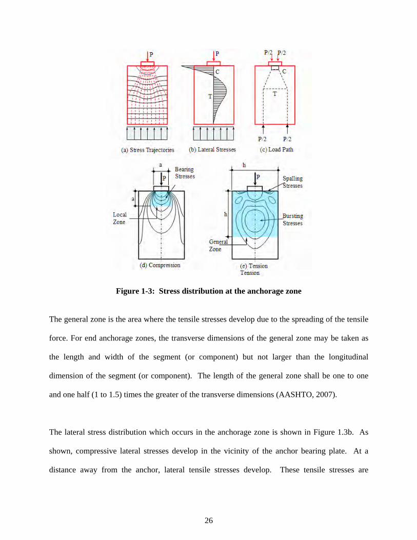
Figure 1-3: Stress distribution at the anchorage zone
The general zone is the area where the tensile stresses develop due to the spreading of the tensile
force. For end anchorage zones, the transverse dimensions of the general zone may be taken as
the length and width of the segment (or component) but not larger than the longitudinal
dimension of the segment (or component). The length of the general zone shall be one to one
and one half (1 to 1.5) times the greater of the transverse dimensions (AASHTO, 2007).
The lateral stress distribution which occurs in the anchorage zone is shown in Figure 1.3b. As
shown, compressive lateral stresses develop in the vicinity of the anchor bearing plate. At a
distance away from the anchor, lateral tensile stresses develop. These tensile stresses are

27
referred to as “bursting stresses”. Reinforcement must be provided to resist the bursting tensile
stresses. Principal compressive and tensile stress contours for a post-tensioning anchorage zone
are shown in Figure 1-3d and Figure 1-3e, respectively. Three critical stress regions which
develop are shown in Figure 1-3d and Figure 1-3e. These are the locations of high bearing
stresses, spalling stresses and bursting stresses.
The anchorage supplier is responsible for providing anchorage devices and information which
complies with AASHTO requirements. The Engineer of Record is responsible for the overall
design of the post-tensioning anchorage zone, both the general zone and the local zone. This
responsibility includes the location of the tendons and anchorage devices, the reinforcement in
the anchorage zone and the tendon stressing sequence. To provide adequate resistance for the
large compressive forces at the anchors and the large tensile forces that develop at a distance
ahead of the anchors, the post-tensioned anchorage zone must be properly designed and detailed.
1.3 Anchorage Zone Reinforcement
If the concrete dimensions are large enough surrounding the anchorage device, adequate
confinement may be provided by the concrete. However, anchorage device suppliers typically
provide spiral reinforcement in the local zone to provide the required confinement for high
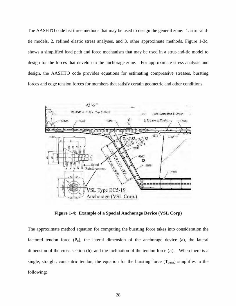
compressive stresses. Figure 1-4 is a cross-section of a bridge box girder segment that shows an
example of a post-tensioning anchorage device (a VSL EC5-19 anchor) and some of the required
steel reinforcement, including the spiral reinforcement in the vicinity of the anchor.
28
The AASHTO code list three methods that may be used to design the general zone: 1. strut-and-
tie models, 2. refined elastic stress analyses, and 3. other approximate methods. Figure 1-3c,
shows a simplified load path and force mechanism that may be used in a strut-and-tie model to
design for the forces that develop in the anchorage zone. For approximate stress analysis and
design, the AASHTO code provides equations for estimating compressive stresses, bursting
forces and edge tension forces for members that satisfy certain geometric and other conditions.
Figure 1-4: Example of a Special Anchorage Device (VSL Corp)
The approximate method equation for computing the bursting force takes into consideration the
factored tendon force (Pu), the lateral dimension of the anchorage device (a), the lateral
dimension of the cross section (h), and the inclination of the tendon force (a). When there is a
single, straight, concentric tendon, the equation for the bursting force (Tburst) simplifies to the
following:

29
Tburst = 0.25 Pu (1- a/h) 1-1
It is the Engineer of Record’s responsibility to design bursting reinforcement to resist the
computed bursting force. Using a reinforcement allowable stress, fs, and a bursting force, Tburst ,
the required area of steel , As, would be computed as follows:
As = Tburst/ fs 1-2
The AASHTO code requires that the bursting steel be distributed such that the distance from the
centroid of the bursting force is equal to dburst. When there is a single, straight, concentric tendon,
dburst is computed by the following equation:
dburst = 0.5h 1-3
1.4 Problems with Anchorage Zones in Bridges
If the post-tensioned anchorage zone is not properly detailed and designed to withstand the
forces and stresses which develop, failure of the anchorage zone can occur. If there is
inadequate confinement reinforcement in the local zone (the vicinity immediately surrounding
the anchorage device) cracking, crushing and spalling of concrete may occur. To prevent failure
in the anchorage zone, non-prestressed (or mild steel) is used to resist the tensile stresses. Due to
the large forces active in the anchorage zones much mild steel is required. Steel congestion in
the area may lead to problems related to poor concrete consolidation.
30
1.5 Fiber Reinforced Concrete
Concrete is a material that is prone to cracking. Research has shown that adding fibers (steel or
polymer fibers) helps to delay the development of cracks and to reduce the size of cracks that do
develop (Khajuria et al, 1991). Since the 1960’s steel fibers have been used in many
construction applications including in shotcrete, precast concrete, concrete slabs, concrete floors
and other applications (Vondran, 1991). Some of the beneficial effects of using fibers in
concrete are enhancing tensile behavior; improving post crack resistance; increasing
development/splice strength of reinforcement; increasing first-crack flexural strength and the
post-cracking flexural stiffness; reducing instantaneous and long term deflections; restraining the
creep of cement matrixes under axial compression; improving creep properties; reducing
shrinkage of cement matrices; and reducing basic creep, shrinkage and total deformation (Tan et
al, 1994).
1.6 Objectives of the Study
The main objective of this research was to investigate the use of steel fiber reinforced concrete
(SFRC) in post-tensioning (PT) anchorage zones of bridge girders. The purpose of using SFRC
is to enhance the overall performance and to reduce the amount of steel rebar required in the
anchorage zone. Reducing steel congestion in post-tensioning anchorage zones can improve the
constructability of post-tensioned bridge elements. Results from an investigation by Haroon
(2003) showed that the use of SFRC improved the local zone capacity and provided a reduction
in secondary mild reinforcement.

31
It was the intent of this study to consider both the behavior of the local zone and the general zone
when steel fiber reinforced concrete is used. Also, It was desirable to implement a test program
that considered material stress levels that are similar to those typically found in post-tensioned
bridge members (such as concrete post-tensioned segmental box girders). To achieve the
objectives of this study, both experimental and analytical investigations were conducted aiming
at reducing the amount of mild steel reinforcement required by the AASHTO code at the
anchorage zone. The experimental part of the study involved laboratory testing of twenty-seven
(27) samples representing typical anchorage zone dimensions in post-tensioned girders. The
analytical study was conducted using non-linear finite element analysis in order to have a
comprehensive stress analysis of the anchorage zones with and without fiber reinforcement and
mild steel reinforcement.
Inherent in the objective is the determination of the proper ratio of steel fibers that can be used
without jeopardizing the constructability of the anchor zone. Meeting the objective of this study
resulted in the development of a rational method to analyze and design the local and general
zones reinforced with steel fibers.

32
CHAPTER 2
LITERATURE REVIEW AND RESEARCH METHODS
Sanders (1990), Stone (1983) and Haroon (2006), reported that failures of the anchorage zones of
precast prestressed concrete girders are brittle in nature. This is the case even when failure is due
to yielding of reinforcing steel. Thus, failure of the post-tensioned anchorage zone should be
avoided. A well designed anchorage zone should safely transfer the tendon forces developed at
ultimate loads such that if a failure occurs in the structures, it is a ductile failure away form the
anchorage zone.
Haroon (2003) reported that, according to Breen et al (1994), cracking rather than complete
failure occurs more frequently in the anchorage zone. Haroon suggests two reasons for this
frequent occurrence; (1) the anchorage zone is inherently tough, and (2) when anchorage zone
fails during construction, the anchorage zone is most likely repaired and not reported as a failure.
To resist tensile forces, a large volume of spiral and other reinforcement may be required at the
end zones of a prestressed bridge girder. Reinforcement congestion in the anchorage zone may
be a cause of poor concrete consolidation, resulting in failures caused by crushing of the concrete
ahead of the anchor (Libby, 1976). As the volume of steel increases in the zone, the difficulty of
placing the steel increases also. In addition, reinforcement components (i.e. anchorage devices
and ducts) used in close proximity cause congestion in the anchorage zone. As a result, it

33
becomes difficult to place concrete, anchorages and post-tensioning ducts in the zone. It is labor
intensive to produce and place secondary anchorage reinforcement. Fiber reinforced concrete
(FRC) possesses better properties, such as tension, compression, shear, bond, flexural toughness
and ductility than conventional concrete. Therefore, it may be possible to utilize FRC in the end
zones of prestressed and post-tensioned bridge girders to reduce the amount of secondary
reinforcement.
2.1 Fiber Reinforced Concrete
Fibers added to concrete could be metallic, polymeric or natural. The metallic fibers have high
modulus and high strength. Their behavior is ductile. Polymeric fibers are strong and ductile but
their modulus is relatively lower than cement composite. Therefore, the addition of polymeric
fibers does not change modulus of elasticity, flexural strength, and compressive strength of
concrete (Berke and Dallaire, 1994).
Fibers in concrete serve mainly three functions: 1) to increase toughness of the composite by
providing energy absorption mechanism related to de-bonding and pull-out processes of the fiber
bridging the cracks, 2) to increase ductility of the composite by permitting multiple cracking, 3)
to increase strength of the composite by transferring stresses and loads across cracks. For fiber
reinforced cementitious composites, load-deflection curves provide information concerning the
effect of the fibers on the toughness of the composite and its crack control potential. The area
under the load-deflection curve represents energy-absorbing capacity. The addition of steel
fibers to concrete improves impact strength, toughness, flexural strength, fatigue strength, crack
resistance and spall resistance (ACI, 2002).

34
Swamy and Al-Ta’an (1982) conducted research to determine the influence of fiber
reinforcement on the deformation characteristics and ultimate strength in flexure of concrete
beams. They tested fifteen (15) reinforced concrete beams. The test parameters included the
fiber content by volume (0.0%, 0.5%, 1.0%) and the use of low carbon crimped steel fibers either
throughout the beam depth or in the effective tension zone only. The researchers concluded that:
(1) steel fibers are effective in resisting deformation at all stages of loading; (2) steel fibers
inhibit crack growth and crack widening; (3) steel fiber reinforced beams showed significant
inelastic deformation and ductility at failure; and (4) steel fibers have limited effect in increasing
flexural strength of reinforced beams.
Bohra and Belaguru (1991) investigated the long term durability of nylon, polypropylene and
polyester fibers in concrete. Specimens with 0.5% fibers (by volume) were stored in lime
saturated water maintained at 50o deg. C. Addition of fibers to the concrete mix resulted in
reduction in slump. In addition, fibers contributed to approximately a 10% reduction in
compressive strength. However, test results indicated that “all three fibers provided post-crack
resistance.” By measuring flexural toughness, the researches found that nylon and
polypropylene fibers are durable in concrete. “Specimens with polyester fibers had lower indices
after accelerated aging.”
Vondran (1991) reported that steel fibers can have up to twice the modulus of rupture, shear
strength, torsional strength, and fatigue endurance; up to 1.4 times the abrasion and erosion
resistance; and up to 5 times the impact energy absorption of plain concrete. He also stated that
35
steel fibers make concrete tougher and more ductile and decrease permeability due to cracking
by preventing microcracks from becoming working cracks.
Shaaban and Gesund (1993) investigated whether consolidation by rodding or vibrating
influenced the compressive strength and split tensile strength of 6”x12” concrete cylinders
containing steel fibers. Acknowledging the sample size was relatively small, the authors
concluded that: 1. “SFRC cylinders tested in compression have essentially the same strength,
whether consolidated by rodding or external vibration.” 2. “Split tensile tests for tensile strength
show significant increases in tensile strength with the addition of steel fibers, and considerably
more strength gain for vibrated specimens than for rodded specimens.” The authors state, “It
also appeared that external vibration produced a more uniform distribution of fibers and fiber
orientations.”
Chaallal et al (1996) conducted a study to compare the performance of steel fiber reinforced
concrete (SFRC) wall/coupling beam joints under cyclic loading with the performance of
conventional reinforced concrete (CRC) joints. The results of the research showed that the
SFRC joint with reduced transverse reinforcement (hoops) performed relatively well. In
particular, the researchers found that the SFRC specimens 1) dissipated 31 percent more energy
than the CRC specimens, 2) improved bond and anchorage of reinforcement, 3) developed more
closely spaced cracks, and 4) showed minimum spalling. The authors concluded that “the use of
SFRC in seismic regions to enhance structural integrity and to ease steel congestion in plastic
hinge regions is potentially viable.”

36
In 1996, the South Dakota (SD) Department of Transportation (DOT), the 3M Company, the
Federal Highway Administration and other entities sponsored an open house in Pierre, South
Dakota to introduce polyolefin fibers to transportation agencies, consultants, concrete suppliers
and academicians. At dosage rates of up to 2% by volume, the addition of polyolefin fibers (2”
long, 0.025” plastic fibers) to concrete was reported to increase concrete ductility, toughness and
resistance to shrinkage and cracking. The South Dakota DOT had used polyolefin fibers in
bridge deck overlays, bridge barriers, concrete paving and bridge deck replacement with good
results.
Harajili and Salloukh (1997) investigated the effect of fibers on the development/splice strength
of reinforcing bars. Using fifteen (15) beam specimens cast without transverse reinforcement in
the constant moment region, differing amounts of tensile reinforcement and fibers (steel and
polypropylene), the researcher tested the beams in flexure. There were six (6) major conclusions
from the research: 1. “Hooked steel fibers considerably increases the development/splice
strength of reinforcing bars in tension”; 2. Steel fibers are more effective in increasing
development/splice strength than transverse reinforcement; 3. Using hooked bars results in more
cracks around spliced bars, less growth of splitting cracks, substantial improvement in the
ductility of bond failure; 4. Polypropylene fibers at 0.6% by volume improved the ductility of
bond failure but were not as effective as steel fibers; 5. The bond strength ratio increases as the
volume fraction of fibers increases, and 6. “Bond tests conducted using pullout specimens
largely underestimate the effect of fibers on the splitting bond resistance of reinforcing bars in
tension.”
37
Bayasi, Gebham and Hill (2004) conducted research on reinforced concrete seismic beam-
column joints. After testing six (6) beam-column joints, the researcher concluded that “addition
of steel fibers to reinforced concrete seismic beam-column joints improves strength, ductility and
toughness of joints. By using steel fibers, hoop spacing in the joint can be relaxed as steel fibers
will have an effect similar to that of reinforcing steel.” According to the recommendation, for
exterior beam-column joints, steel fibers at a volume fraction of 2% can be used with a code
hoop spacing increased by a factor of 2. For high seismic risk areas, it was recommended that in
a SFRC joint, the hoop spacing could be increased by a factor of 1.5. In summarizing literature
on beam-column joints published by other researchers from 1974 to 1992, the authors noted that
the consistent findings were that joints reinforced with steel fibers had higher ultimate moment
capacity, increased ductility, increased cumulative energy dissipation, improved ultimate rotation
capacity, improved stiffness, less spalling, better confinement, better crack control, higher shear
strength, increased tensile strength and increased bearing strength (Bayasi et al, 2004).
Tan et al (1994) investigated instantaneous and long-term deflection of steel fiber reinforced
concrete beams. A total of fourteen (14) beams were tested: four to failure under third point
loading and nine (9) under long term creep tests. Fiber content was varied from 0.55 to 2.0%.
Two of the conclusions from the research were: “1. The inclusion of steel fibers was found to
result in an increase in first-crack flexural strength and post-cracking flexural stiffness of
reinforced concrete beams. 2. Both the instantaneous and long-term deflections of SFRC beams
were smaller than comparable plain concrete beams.”

38
2.2 Fiber Reinforcement in Prestressed Concrete
Wafa (1992) tested 18 axially prestressed and non-prestressed concrete beams subjected to
torsion. The variables included prestressing levels and fiber volumes (0.0% to 2.0%). The
researcher concluded that in torsion, “beams without fibers have practically no ductility and
failure is sudden and violent. Addition of fiber beyond 1 percent [1%] increases ductility and
torsional strength”. However, for fiber volumes less than 1%, “there is practically no increase in
the torsional strength”.
Junior and Hanai (1999) tested nine (9) concrete beams to investigate the influence of steel and
polypropylene fibers on shear performance of thin-walled I-beams with reduced shear
reinforcement. Variables for the beams included prestressing, no prestressing, shear
reinforcement ratios, amount and type of fibers. The authors found that fiber reinforcement
contributed to more effective crack control and smaller deflections. For beams with stirrups,
the presence of fibers resulted in increased shear strength after first cracking and decreased
deflection. However, these beneficial effects did not occur in beams without stirrups. According
to the authors, increases in strength in the fiber reinforced beams varied from 13% to 19%. One
conclusion reached by the authors is that “the contributions of fibers can be considered
equivalent to a fraction of the shear reinforcement” … which “confirms the possibility of an
advantageous partial substitution of stirrups for fibers.”
The authors made reference to ACI Committee 544 and work by Shah and Ouyang. Junior and
Hanai stated, “The use of short fibers in concrete offers noticeable advantages such as limited
cracking and increases toughness. It can also increase shear strength, allowing reduction of

39
stirrup reinforcement, and improved ductility and safety.” Two of the main conclusions from
the research related to fiber reinforcement were as follows: 1. “The addition of fibers does not
increase the compressive strength of concrete, but it can increase tensile strength in some cases.
The modulus of elasticity of concrete can be altered with the introduction of fibers”; 2. “Fiber
effectiveness is higher in beams with stirrups. In all the fiber reinforced beams failure was more
ductile and there was increased strength, always between 8 and 10 kN. The fibers can be
considered as equivalent shear reinforcement. In this aspect, the advantages provided by steel
and polypropylene fibers were similar, but the strain in the stirrups in steel fibers beams was
smaller.”
2.3 Post-Tensioned Anchorage Zones
The development of post-tensioning as one method of prestressing concrete occurred after 1923.
Franz Dischinger designed the first prestressed concrete bridge which was built in Aue, Germany
in 1937 (Hengprathanee, 2004). After the bridge at Aue was constructed, the Dywidag post-
tensioning system was invented by Ulrich Finsterwalder in the 1940’s (Hengprathanee, (2004).
Since the 1940’s, post-tensioning has been used in concrete bridges. The first use of post-
tensioned concrete in the United States was in the Walnut Bridge which was constructed in
Philadelphia in 1950 (Podolny and Muller, 1982). The Walnut Lane Bridge was a cast-in-place,
post-tensioned bridge.
Concrete structural members are prestressed to increase their load carrying ability and improve
their behavior under loading. Post-tensioning is one of two methods (pre-tensioning and post-
tensioning) for prestressing concrete structural elements. In post-tensioning anchorage zones

40
high stresses develop due to the transfer of prestressing force through bearing plates and anchors.
To prevent these stresses from causing splitting, bursting and cracking of the concrete in the
anchorage zone, adequate detailing is required. This detailing includes provision of sufficient
concrete volume and reinforcing steel in the high stress region. Design specifications, anchorage
devices, and design experience are all important for successfully designing and detailing of
anchorage zones.
In 1956, Huang wrote the following: “Although, the post-tensioning method for prestressing
concrete structural members has been used by engineers for thirty years, literature concerning the
end block stresses has been remarkably scarce. In 1946, Professor Mangel made probably the
first publication dealing with the problem.”
If Huang’s statement is accurate, then the design and behavior of post-tensioning anchorage
zones have been an area of concern for over 60 years. While some design guidance was
provided by researchers such as Guyon, Morsch and Leonhardt, codified design procedures were
lacking for a long period of time. The Post-Tensioning Institute first published its Post-
Tensioning Manual in 1972. The American Association of State Transportation Officials
(AASHTO) did not include post-tensioning anchorage design guidelines in its bridge design
specifications until 1994 (Roberts-Wollman and Breen, 2000). This specification resulted from
research conducted by Breen et al (1994) at the University of Texas at Austin.
Huang noted that although the end block (anchorage zone) problem was a three dimensional
problem most of the existing methods for analyzing the end blocks treated the problem as two

41
dimensional by neglecting forces in the vertical direction. These often neglected forces included
the beam support reaction, the dead and live load applied over the anchor block, the weight of
the end block, and the vertical force of an inclined cable. In his investigation, Huang sought to
consider the “actual” distribution of stresses in the end block by using experimental and
analytical methods (Huang, 1956).
To complete his study, Huang instrumented and tested one post-tensioned beam and completed a
two-dimensional numerical analysis. The test beam was modeled based upon a beam with a fifty
(50) foot span. To represent the two end zones, a 9’-6” beam was instrumented, post-tensioned
and loaded. The concrete compressive strength, f’c, of the beam was 6000 psi. Even though
Huang’s study was limited and problems developed with some of the strain gages, he noted that
the existing methods for designing the end block gave “quite different” results from his
experimental and analytical results. He compared his results to design methods proposed by
Guyon, Mandel and others. Huang made four (4) conclusions: 1. For the end block, the optimum
length-depth ratio is probably close to one; 2. To prevent failure in the end zone, vertical and
horizontal reinforcement should be used for a distance of one end block length away from the
load surface; 3. “The horizontal normal stress (parallel to the tendon)…may be assumed to
follow a linear vertical distribution with sufficient accuracy, but laterally, its distribution is better
approximated by a parabola; 4. While some of the other loads in the end zone can be neglected,
“the reaction from the end support and the vertical shear at the juncture should be considered.”
Saadoun (1980) completed a three dimensional photoelastic investigation of the end block. His
investigation considered single and multiple anchorages, external and embedded ducts and end

42
blocks with and without ducts. In addition, he conducted tests on concrete end block models.
Some of his conclusions were as follows:
o High sub-surface shears in the vicinity of the anchorage unit [device] initiate a punching
shear type failure and the subsequent propagation of tensile cracks in a complex
compression-tension stress field caused by wedging action of the concrete cone governs
the failure of the end block”
o For external anchorage end blocks, the sub-surface shear stress reach a maximum value
of three times the mean compression that occurs just beneath the edge of the loaded area
o All two-dimensional theoretical solutions underestimate the critical tensile stresses and
forces and completely overlook the real significance of the high sub-surface shears in the
immediate vicinity of the anchorage units
o The photoelastic methodology provides a realistic picture of the nature of magnitude and
stress distribution and that the Poisson’s ratio differential effect is small”
o Tensile zones were found in the corners of end blocks, the spalling zones and between the
anchorage units

43
o One third of the load applied at the embedded anchorage unit was transmitted through
shear tractions on the longitudinal surface of the anchorage unit. This leads to a reduction
in the level of the maximum tensile stresses and forces
o The maximum transverse tensile forces for the embedded anchorage were only 65 to 70%
of the corresponding values for the external anchorage units
Burdett’s (1990) research included a comparison of existing codes and design guidelines for the
design of anchorages zones. According to Burdett, most of the codes reviewed did not
distinguish between the local and the general anchorage zones. However, the codes did limit the
bearing stresses under the anchorage device and did give some estimate of the tensile bursting
forces. Most formulas for bursting force that Burdett reviewed were in the form of :
F = K P (1 - a1/a2) 2.1
where F = the bursting force, K= a factor between 0.25 and 0.3, P = the tendon force, a1 = the
dimension of the anchorage device and, a2 = the lateral dimension of the member. As reported
by Burdett, Guyon proposed a linear approximation defined by the equation:
Tburst = 0.3P (1-a/h) 2.2
44
where P = the tension force, a= the dimension of the anchorage plate, and h= the depth of the
section. In addition, Burdett noted that most of the design codes gave maximum values for the
maximum tensile stress in the range of 0.5(f’c )1/2 to 7.5(f’c )1/2.
In addition to reviewing existing codes, Burdett conducted finite element analysis (FEA) of the
anchorage zone and evaluated strut-and-tie (SNT) models of the zone. His findings included the
following:
1. The bursting stresses obtained from the FEA, showed good agreement with other
solutions;
2. The stress distribution was closest to the elastic solution obtained by Guyon;
3. Using a factor of 0.25 instead of 0.3 resulted in a better fit of the FEA results, but the
values were smaller than the predicted values for plate sizes smaller than 0.15h;
4. Values of the spalling force obtained from the finite element analysis showed that the
constant value for spalling forces equal to 4% of the applied load proposed by Guyon is
conservative;
5. Stresses from the FEA are reliable and accurate;
6. The strut-and-tie Model results were in close agreement with the finite element method
results.
The investigation conducted by Burdett was part of a comprehensive research program
completed at the University of Texas at Austin to help improve the AASHTO specifications and
provide design guidance for bridge post-tensioned anchorage zones. This research was
sponsored by the Transportation Research Board’s (TRB) National Cooperative Highway

45
Research Program. Other UTA researchers involved with this study included J. E. Breen, C.
Roberts, D. Sanders and G. Wollman (Breen et al, 1994). As a result of this research program,
the team proposed anchorage design specifications for AASHTO. These proposed specifications
included practical design formulas for the tensile bursting force and for the location of the
centroid of the tensile stresses:
Tburst = 0.25(1-a/h) +0.5Psin(α) 2.3
dburst = 0.5(h-2e) + 5 e sin(α) 2.4
where P = the total factored tendon load, a= the lateral dimension of the anchorage device or
group of devices, e = the eccentricity of the anchorage device or group of devices, h= the
transverse dimension of the cross section, and α = the inclination of the resultant of the tendon or
tendons with respect to the centerline of the member. In addition to the equations, the proposed
specification, recommended the subdivision of the anchorage zone into a local zone and a
general zone.
Roberts (1990) conducted research to examine acceptance test procedures for post-tensioning
systems, to consider the performance of post-tensioned anchorage local zones and to propose
specifications for design and construction of anchorage zones. Roberts conducted anchorage
tests using several different testing procedures for acceptance of anchorage hardware. She
evaluated four different testing procedures including the ones recommended by the following
entities:
1. the European FIP code,

46
2. the Post-Tensioning Institute
3. the German DIN code and
4. the Austrian Code
As a result of load tests and evaluations of the existing codes, Roberts proposed a rectangular
prism test block for the local zone. The cross-sectional dimensions of the block were to be
related to the edge distance or minimum spacing of anchors (the smaller of the values) and the
length of the block was to be two times the longer of the cross-sectional dimensions.
In addition, to proposing the test specimen, she proposed a procedure and criteria for acceptance.
Some of her research conclusions were as follows:
1. “The primary parameters which affect the first cracking load are the tensile capacity of the
concrete and the a/h ratio”;
2. An increase in spiral diameter
a) does not increase first cracking load,
b) does not significantly decrease crack widths,
c) does increase the ultimate load, and
d) does increase the ultimate deformation capacity of the specimen.
In summary, Roberts states, “The behavior of the local zone is primarily a function of the A/Ab
ratio, the area confined by the primary confining reinforcement, and the volumetric ratio of the
reinforcing steel to the confined concrete. The interaction of these variables dictates the overall
local zone behavior.”

47
Sanders (1990) conducted a study to develop a generalized approach for the design and proper
reinforcement of post-tensioned anchorage zones. He performed load tests and developed strut-
and-tie model for the research. He performed experimental tests (load tests) on thirty-six (36)
specimens representing different types of anchorage zones: zones with eccentric, concentric,
multiple and inclined tendons. As a result of his work, he developed a modified strut-and-tie
model which “more accurately represents the ultimate behavior and capacity of the anchorage
zone” (Sanders ,1990). The results of his work were used to help develop the AASHTO
specifications for post-tensioned anchorage zones.
Using finite element models, strut-and-tie models and experimental tests, Wollman (1992)
investigated post-tensioned anchorage zones as a part of the research conducted at the University
of Texas at Austin. Wollman concluded that both strut-and-tie models and finite element
analysis can be safely used to design post-tensioned anchorage zones. According to Wollman,
the strut-and-tie models gave conservative predictions for failure loads. Also, he concluded that
the magnitude and location of bursting forces and bursting stresses are affected by the presence
of reaction forces in the anchorage zones. However, the influence of the reaction forces is
conservative and may be neglected for small tendon eccentricity and in the absence of flexural
tensile stresses at the end of the anchorage zone (Wollman, 1992).
The Post-Tensioning Institute published a document entitled Anchorage Zone Design which was
authored by Wollman and Robert-Wollman (2000). This publication provided post-tensioned
anchorage zone design guidance and examples for design professionals.

48
Jo, Byun and Tae (2002) modeled the post-tensioned anchorage zone of a cable-stayed bridge.
They used three-dimensional and two-dimensional finite element models to investigate the stress
distribution in the anchorage zone. Study parameters included the cable inclination, the position
of the anchor plate, the modeling methods and three-dimensional effects. Jo et al reported that
Leonhardt provided an equation for computing the transverse tensile force, T, in 1964. The
Leonhardt equation is as follows:
T = 0.3 ∑ P (1-a/h)+0.5 |∑ Pu sin α| 2.5
where P = the maximum prestressing force due to post-tensioning, a=the anchor plate width, h =
the member depth, Pu = the factored tendon force and α = the angle of inclination of the tendon
force. As can be seen by comparison, this equation is very similar to the equation that is
presented in the AASHTO design specifications for computing Tburst. Two of the conclusions
made by Jo et al were as follows: 1. The inclination of the cable influences the stress distribution.
The maximum bursting stress increases when the cable inclination angle becomes acute; 2. Since
the three-dimensional analysis showed slightly less [stress] values for the anchorage [zone] than
the two-dimensional analysis, for simplicity in analysis and safety in design, two-dimensional
analysis can be used.
Haroon (2003) investigated the feasibility of using steel fibers to reduce the amount of steel
reinforcement in post-tensioned anchorage zones. He performed material tests with concrete
containing Xerox steel fibers, Dramix ZP305 steel and Harbourite H-330 synthetic fibers. For the
material tests, Haroon considered fiber volume percentages of 0.5%, 0.75% and 1.0%. In

49
addition to the material test, Haroon performed AASHTO Special Anchorage Device Acceptance
Tests for 12.5”x12.5”x25” concrete specimens cast with VSL EC 5-7 anchorages and Xerox and
Dramix ZP305 steel fibers. In the test blocks Haroon used 0.75% and 1.0% fibers (by volume).
Cyclic loading tests were performed on the test blocks to evaluate local anchorage zone
reinforcement. Thirty-seven (37) anchorage test blocks with different amounts of spiral
reinforcement, tie reinforcement and steel fiber reinforcement were tested. To help verify test
results, Haroon performed a finite element analysis of the test block. As a result of his research,
Haroon concluded that adding steel fibers increased the concrete 1) compressive strength, 2)
tensile strength, 3) flexural first crack strength and 4) post-crack energy absorption capacity.
Based upon his tests results, Haroon recommended that steel fiber reinforced concrete (SFRC) be
used in the end zones of prestressed girders to reduce or eliminate secondary reinforcement (i.e.
steel spirals and/or tie reinforcement). He stated, ”from the reinforcement congestion
perspective, elimination of the spiral steel is more beneficial than the elimination or reduction of
skin reinforcement [steel ties]”.
Hengprathanee (2004) used the DIANA finite element analysis program to conduct linear and
nonlinear finite analyses of the post-tensioned anchorage zones. He considered the presence of a
support reaction in the anchorage zone and post-tensioning tendons with different configurations
(concentric, eccentric, inclined and inclined eccentric). In addition, he considered strut-and-tie
models for design of anchorage zones. As a result of his research, Hengprathanee proposed a
new approach for the design of non-rectangular anchorage zones. This new approach was based
upon a modified version of the strut-and-tie model. For the reaction forces in the rectangular

50
anchorage zones, Hengrathanee proposed a modification to the AASHTO code equations for
Tburst and dburst.
Tburst = 0.25 ∑ Pu (1-a/(h-2e))+0.4 ∑(Pu sin α)+ R(0.25- 5 sin α)>= 0.125 ∑Pu 2.6
dburst = 0.5 (h -2e)+ 0.25a+0.25 (h-2e) sin α + (R /(∑Pu)) (h -2e) (1.5-10 sin α) 2.7
where Tburst = tensile force; Pu =factored tendon force; dburst = the distance from the anchorage
device to the centroid of the bursting force, Tburst; α = the lateral dimension of the anchorage; e=
the eccentricity of the anchorage; h=the lateral dimension of the anchorage zone in the direction
considered; a= the angle of inclination of the tendon force; and R= the reaction force applied at
the bottom surface of the anchorage zone.
Johnson (2006) completed a finite element analysis model of a post-tensioned (PT) anchorage
zone for one of the box girder anchor segments of the Mid-Bay Bridge which is located in
Florida. The finite element model of the Mid-Bay Bridge segment was used to evaluate the size
of PT anchorage test specimen for the experimental program and the percentage of steel fiber to
use in the anchorage load test program for this study.
2.3.1 Post-Tensioning Systems
Two of the post-tensioning anchorage systems used in the United States of America are the VSL
Post-Tensioning System and the Dywidag Post-tensioning System. The Dywidag System was
developed in the 1940’s. “The VSL Post-Tensioning Systems have been used throughout the
world since 1956 (VSL Corporation, 1996)”. While the two systems are similar, the anchorage

51
devices for each system are unique. Post-tensioned anchorages from these two systems are used
in this research program. Specifications for the two systems are given in Chapter 5.
2.3.2 Stress Distribution for Post-Tensioning Anchorage Zones
Research has shown that a transverse bursting force develops in the anchorage zone a distance
away for the end of a beam where the post-tensioning force is applied to the beam. This tensile
force is transverse to the path of the tendon. The force must be resisted by steel reinforcement.
The total area of steel that is required to resist this force can be computed by dividing the
magnitude of the tensile force by the allowable stress of the reinforcement: As= T/fs, where T is
the tensile force, fs is the allowable stress of the reinforcing steel and As equals the area of steel
required to resist the bursting force. The area of the bearing plate of an anchorage device must
be adequate to satisfy the AASHTO code requirements, including the concrete compressive
stress limit of Section 5.10.9.6.2.
2.3.3 Post-Tensioned Anchorage Zones in AASHTO Design Specifications
According to the AASHTO code (2007), “anchorage and couplers are to develop at least 95% of
the minimum specified ultimate strength of the prestressing steel without exceeding the
anchorage set movement assumed for the design. Unbonded systems are also to pass a dynamic
loading test.” In addition, at critical sections, the strength required of bonded tendon can not
exceed the resistance of the tendon assembly (anchorage or coupler). In Section 5.4.6, AASHTO
provides guidelines for the size and alignment of ducts. The radius of curvature of tendon ducts
in the anchorage areas shall not be less than 12.0 ft. “The size of the duct shall not exceed 0.4
times the least gross concrete thickness at the duct (AASHTO, 2007).”

52
Section 5.10.9 of the code defines anchorage zone dimensions for end anchorage zones and
intermediate anchorage zones. The coded states that for design purposes the anchorage zone
comprises two regions: the local zone and the general zone. The Engineer of Record is
responsible for the design of the anchorage zone. Section 5.10.9.3.1 list three methods that may
be used for the design of the general zone: 1. strut-and-tie models, 2. refined elastic stress
analyses and 3. other approximate methods.
For certain conditions or limitations, the AASHTO code provides equations for estimating
concrete compressive stresses, the location and magnitude of the bursting force, and the edge
tension in post-tensioned anchorage zones in Section 5.10.9.6, Approximate Stress Analyses and
Design. The AASHTO equations for the location and the magnitude of the bursting stresses are
as follows:
Tburst = 0.25 Σ Pu (1-a/h) +0.5|Σ(Pu sin α)| 2.8
dburst = 0.5(h-2e) + 5 e sin α 2.9
In these equations, Tburst =tensile force (or bursting force) in the anchorage zone; Pu=factored
tendon force; dburst =the distance from the anchorage device to the centroid of the bursting force,
Tburst; a = the lateral dimension of the anchorage; e=the eccentricity of the anchorage; h =the
lateral dimension of the anchorage zone in the direction considered; α=the angle of inclination of
the tendon. These equations were considered in the evaluation of the performance of the post-
tensioned anchorage zone with steel fiber reinforced concrete (SFRC).
53
2.4 Research Methods
In the conduct of this research, the work performed included 1. testing materials; 2. load testing
twenty-seven (27) anchorage specimens; 3. using the finite element method to model test
specimens; 4. using empirical equations for computing forces and stresses; and 5) comparing all
test, finite element results and empirical results. Compressive strength, tensile strength, flexural
strength and modulus of elasticity tests were performed for concrete with and without steel
fibers. The actual mix design used for this research project is similar to one recommended by the
Florida Department of Transportation (FDOT) Materials Laboratory. This concrete mix was a
high slump mix design. A 4000 psi concrete mix was used because this is the minimum concrete
strength recommended by VSL, a post-tensioned anchorage manufacturer. For example,
although VSL’s literature states that “maximum prestressing force may be applied when concrete
reaches a cylinder strength of 3500 psi”, the VSL anchorage device dimensions are valid for a
nominal concrete cylinder strength at 28 days of 4000 psi.
The three (3) fibers used in the research project were Dramix ZP305, Helix, and Novomesh 850.
In the initial stages of this research project, Helix was a relatively new product consisting of
“twisted polygon shaped high tensile steel wires” (Polytorx). Novomesh 850 is a combination of
steel and polypropylene fiber blend.
To help determine the types and percentages of steel fiber that could improve the performance of
the post-tensioned anchorage zone, material tests were performed. Tests were performed for
plain concrete and for concrete containing each of the three fibers (Dramix, Helix and
Novomesh). The fiber percentages used varied from 0.25% to 1.0% by volume. Based upon

54
research by Haroon (2003), a 1.0% fiber percentage was originally considered for use for each
anchorage specimen. However, finite element analysis and material tests were performed before
the load test specimens were cast. The fiber percentage selection was made as a result of
considering 1) recommendations from the fiber manufacturers, 2) finite element analysis results,
and 3) material test results. The dosage of 0.5% fiber by volume was selected for the fiber
percentage (by volume) to use in the anchorage test specimens in this research program.
One (1) anchorage test specimen size was used in the load test program. The size of the
anchorage test specimens was based upon the definition of the general post-tensioning anchorage
zone and the AASHTO code. A review of several box girder bridges that have been constructed
in the State of Florida was considered also. These bridges included the Santa Rosa Bay Bridge
(BR# 580174), Choctawhatchee Bay Bridge (Mid-Bay, BR#570091), and SR-600 Bridge (BR#
790187 & 790188). However, the initial geometry of the proposed test specimen was based
primarily upon two main sources of information: 1) the joint manufacturer’s recommendations
concerning minimum edge distances and minimum anchor spacing, and 2) the AASHTO code
definitions of local and general post-tensioning zones and the geometry limitations for use of the
AASHTO “Approximate Method” for designing post-tensioning anchorage zones.
The adequacy of the specimen size was verified twice by using finite element analyses. The first
round of finite element analysis was done on a typical segment of MidBay Bridge where stresses
at the PT anchorage zone were determined and compared with the anticipated stresses from the
proposed laboratory test specimens. Also, the geometry and the boundary conditions of the tested
specimen were obtained based on the distribution of the tensile stresses in the PT anchorage
55
zone. Another round of FEA was conducted after the completion of the laboratory testing
program. This round was needed to compare the strain measurements from tested specimens with
those predicted from the first round of FEA. Additionally, a parametric analysis was done to
obtain a modified relationship for determining the bursting forces in PT anchorage zone when
SFRC is used.
Section 5.10.9.6.1 of the 2007 AASHTO code lists conditions that must be true for stresses and
forces to be estimated using the approximate stress analyses and design equations. One of the
conditions stated in AASHTO Section 5.10.9.6.1 is that “the minimum edge distance of the
anchorage in the main plane of the member is not less than 1.5 times the corresponding lateral
dimension, “a”, of the anchorage device.” The size of the load test specimens used in this
research was based upon having two (2) VSL EC 5-7 anchorage devices embedded in each
specimen.
In this study, the stress distribution at the anchorage zone was investigated using ANSYS
software program. Several models were produced to simulate the laboratory test samples. Using
finite element analysis results, plots of transverse stresses were used to obtain transverse forces
for specimens with different percentages of fiber and anchor plate to transverse depth ratios
(a/h). Based upon empirical equations presented in the AASHTO code for post-tensioning
anchorage zones, transverse tensile forces were calculated. The calculated forces were compared
to the FEA results. In addition, compression and tension forces anticipated in the post-tensioning
anchorage zone were computed using the strut-and-tie method. The transverse tensile forces
calculated by the strut-and-tie method were compared to the test results and the finite element

56
results. Based upon the research, a new equation was proposed for computing the transverse
tensile forces. This equation takes into consideration the percentage of steel fibers used in the
concrete.
Chapter 3 discusses in detail the materials test program. Chapter 4 presents the anchorage test
program parameters considered in casting twenty-seven (27) anchorage specimens and the
laboratory load test results for each of the twenty-seven (27) load test specimens. Chapter 5
presents all the results from the testing program with descriptions of the behavior of each
specimen during testing.. In Chapter 6, numerical calculations based upon the AASHTO code,
experimental results, and finite element analysis results are compared with the laboratory test
results. An approximate cost comparison for using reinforced concrete and fiber reinforced
concrete in post-tensioned anchorage zones is also given in Chapter 6. Finally, Chapter 7
contains conclusions and recommendations resulting from the research program.

57
CHAPTER 3
MATERIALS TESTING
To help determine acceptable fibers and percentage of fibers to use in the anchorage load test
program, extensive materials testing was performed. The materials test program considered a
4000 psi mix design, three (3) different fibers, and a range of fiber percentages: 0%, 0.25%,
0.33%, 0.5%, 0.75% and 1.0%. To investigate materials properties for the fiber reinforced
concrete, compressive strength, tensile strength and flexural strength tests were conducted from
“preliminary” concrete batches which were cast before anchor test specimens were cast. In
addition to conducting material tests from the preliminary concrete batches, sixteen (16) 18” x
18” x 2.5” concrete slabs were cast to help evaluate cracking resistance.
In this chapter the materials used in the testing program are described. After the preliminary
material tests were conducted, twenty-seven (27) anchor test specimens were cast. For these
specimens, additional compressive strength, tensile strength and modulus of elasticity tests were
performed. The material test results for the anchorage test specimens are included in this
chapter. However, the selection of the geometry and the fiber contents of the anchorage test
specimens are described in detail in Chapter 4. In Chapter 4, the load test results for the
anchorage test specimens are presented and discussed.

58
3.1 Concrete Mix Design
A 4000 psi concrete mix was used because the minimum concrete strength recommended by one
post-tensioned anchorage supplier (VSL) is 4000 psi. Recognizing that the inclusion of steel
fibers in the concrete mix would result in a decrease in workability, a high slump concrete mix
was selected. Thus the 4000 psi concrete mix design that was selected had 7 to 9 in slump.
Detailed design mix is shown in Table 3-1.
Table 3-1: 4000 psi Concrete Mix Design
Specifications for Mix Design of f’c = 4000 psi. Slump 7-9 in, Air Content = 0 to 6.0%
Component Specification 1 y3
Cement (lb) Suwannee American (AASHTO M-85-Type II) 509 Coarse Aggregate (lb) E. P. Jahna (57 SG, 2.53 SSD) 1638 Pine Aggregate (lb) Crowder Sand (2.55 50, 2.64 SSD) 1092 Air Entrainment Admixture (oz) AEA 92 Euclid (AASHTO M-154) 1.9 WPDA 64 Admixture (oz) Eucon WP Euclid (AASHTO M-194 Type D) 45.6 Fly Ash (lb) Boral (ASTM 0-618 Class F) 251 Water (gal (lb)) Potable 34.5 (287.5)
3.2 Material Tests
The three (3) fibers used in the research project are Dramix ZP305, Helix, and Novomesh 850.
Dramix ZP305 (a steel fiber with bent ends) was used in earlier tests conducted by Haroon
(2003). Helix is a product consisting of twisted polygon shaped high tensile steel wires.
Novomesh 850 is a steel and polypropylene blend. Although a 1% fiber percentage was
originally considered due to results of the research conducted by Haroon (2003), material test
specimens were cast with different amounts of fibers (0.0%, 0.25%, 0.33%, 0.5%, 0.75% and

59
1.0% by volume). Figure 3-1 shows the three types of fibers used in this study. Table 3-2
describes the properties of these fibers
Figure 3-1 Steel Fiber (a) Dramix ZP305 (b) Helix (c) Novomesh 850
Table 3-2: Steel Fiber Information
Fiber Information
Fiber L (in) Steel Dia. Steel Aspect Ratio
Steel Tensile Strength
Deformation
Recommended Dosage Range and Recommended Concrete Slump
Dramix ZP305
1.18 in (30 mm)
0.02 in (0.55 mm)
55
Min. 145 ksi (1100 N/mm2)
Hooked ends
Less than 2% by Volume- Recommended maximum Dosage based upon 8 mm max aggregate size: 110 kg/m3 (185 lb/y3)
Helix 1 in 0.02 in 50 Twisted
polygon shape 5 to 66 lb/CY ≈ 0.04% to 0.5%
Novomesh 850
1.5 in 34 140-180
ksi
Continuously Deformed Circular Segment
24 to 48 lb/CY ≈ 0.18% to 0.35%

60
3.3 Material Test Results for S1 and S2 Anchorage Specimens
A total of 27 batches of concrete were cast to investigate material properties prior to the casting
of the anchorage test specimens. Ready-mix concrete was used in Concrete Batches 1 through 4.
The ready-mix concrete was mixed and delivered to the FAMU-FSU College of Engineering by
a ready mix vendor. Based upon the material test results and the finite element analysis, the size
of the anchorage block specimens was decided. Finally, another 8 batches of concrete were
mixed and 27 anchorage test specimens using 0.5% fibers by volume were then prepared for
laboratory testing. Concurrently, cylindrical samples were prepared from the last 8 batches to
determine the compressive strength and the split tensile strength of the concrete. Additional
information about concrete mix design for the 35 batches is shown in Table 3-3 to Table 3-9.
Table 3-3: Concrete Batches 1 to 5
Batch Number 1 2 3 4 5 Batch Source TRM TRM TRM TRM FAMU Cast Date 2/28/06 3/1/06 3/2/06 3/3/06 4/18/06 Amount Made (yd3) 2.5 1.0 2.0 2.0 0.18 Cement (lb) 1265 565 1105 1045 91.62 Coarse Aggregate (lb) 4450 2110 3440 3360 294.84 Fine Aggregate (lb) 2780 1110 2370 2240 197 Flyash (lb) 610 255 505 510 45.18 Euclid, Air Entrainment (ml) 5 91 3 3 10.3 Euclid, Water Reducer (ml) 228 182 182 246.3 Superplasticizer (ml) 0 0 0 0 0 Water 28 gal 19 gal 17 gal 51.75 lb Water Cement Ratio (w/c) .18 .15 .14 0.38 Slump Before Fiber (in) 7.5 5 7.5 7.0 9.5 Slump After Fiber (in) 4.5 Fiber Helix Helix Dramix Novomesh NONE
Plain Plain D.25 N.25 Plain H.25 H.75 D.36 N.36 H.36 H1.0 D.50 N.50 H.50 Beams D.75 N.75
Specimens Cast
Slabs D1.0 N1.0

61
Table 3-4: Concrete Batches 6 To 10 Batch Number 6 7 8 9 10 Batch Source FAMU FAMU FAMU FAMU FAMU Cast Date 4/28/06 4/30/06 5/1/06 5/2/06 5/2/06 Amount Made (yd3) 0.10 0.10 0.10 0.10 0.10 Cement (lb) 50.9 50.9 50.9 50.9 50.9 Coarse Aggregate (lb) 163.8 163.8 163.8 163.8 163.8 Fine Aggregate (lb) 109.2 109.2 109.2 109.2 109.2 Flyash (lb) 25.1 25.1 25.1 25.1 25.1 Euclid, Air Entrainment (ml) 6 6 6 6 6 Euclid, Water Reducer (ml) 135 135 135 0 0 Superplasticizer (ml) 0 0 0 450 450 Water (lb) 28.75 28.75 28.75 28.75 28.75 Water Cement Ratio (w/c) 0.38 0.38 0.38 0.38 0.38 Slump Before Fiber (in) 5.75 4.75 10.25 9 Slump After Fiber (in) 4.25 0.5 0.375 4.0 2.75 Fiber Dramix Helix Novomesh Dramix Helix Fiber (lb) 13.2 13.2 13.2 13.2 13.2 Specimens Cast D1.0 H1.0 N1.0 D1.0 H1.0
Table 3-5: Concrete Batches 11 to 15 Batch Number 11 12 13 14 15 Batch Source FAMU FAMU FAMU FAMU FAMU Cast Date 5/3/06 5/3/06 5/4/06 5/5/06 5/5/06 Amount Made (yd3) 0.10 0.10 0.10 0.10 0.10 Cement (lb) 50.9 50.9 50.9 50.9 50.9 Coarse Aggregate (lb) 163.8 163.8 163.8 163.8 163.8 Fine Aggregate (lb) 109.2 109.2 109.2 109.2 109.2 Flyash (lb) 25.1 25.1 25.1 25.1 25.1 Euclid, A. E. (ml) 6 6 6 6 6 Euclid, W. R. (ml) 0 0 0 0 0 Superplasticizer (ml) 650 450 550 450 225 Water (lb) 28.75 28.75 28.75 28.75 28.75 Water Cement Ratio (w/c) 0.38 0.38 0.38 0.38 0.38 Slump Before Fiber (in) 8.75 9.0 8.5 11 10.5 Slump After Fiber (in) 0.75 6.5 3.75 9.75 9 Fiber Type Novomesh Dramix Helix Novomesh NovomeshFiber (lb) 13.2 6.6 6.6 6.6 4.8 Specimens Cast N1.0 D.50 H.50 N.50 N.36

62
Table 3-6: Concrete Batches 16 To 20 Batch Number 16 17 18 19 20 Batch Source FAMU FAMU FAMU FAMU FAMU Cast Date 5/7/06 5/7/06 5/8/06 5/10/06 5/10/06 Amount Made (yd3) 0.10 0.10 0.10 0.10 0.10 Cement (lb) 50.9 50.9 50.9 50.9 50.9 Coarse Aggregate (lb) 163.8 163.8 163.8 163.8 163.8 Fine Aggregate (lb) 109.2 109.2 109.2 109.2 109.2 Fly ash (lb) 25.1 25.1 25.1 25.1 25.1 Euclid, Air Entrainment (ml) 6 6 6 6 6 Euclid, Water Reducer (ml) 0 0 135 135 135 Superplasticizer (ml) 225 225 0 0 0 Water 28.75 28.75 28.75 28.75 28.75 Water Cement Ratio (w/c) 0.38 0.38 0.38 0.38 0.38 Slump Before Fiber (in) 10.25 10.75 10.25 9.5 8.75 Slump After Fiber (in) 9.5 10.5 8.5 7.0 5.75 Fiber Helix Dramix Helix Novomesh Dramix Fiber (lb) 4.8 4.8 9.9 9.9 9.9 Specimens Cast H.36 D.36 H.75 N.75 D.75
Table 3-7: Concrete Batches 21 To 25 Batch Number 21 22 23 24 25 Batch Source FAMU FAMU FAMU FAMU FAMU Cast Date 5/12/06 5/12/06 5/12/06 5/16/06 5/16/06 Amount Made (yd3) 0.10 0.10 0.10 0.10 0.10 Cement (lb) 50.9 50.9 50.9 50.9 50.9 Coarse Aggregate (lb) 163.8 163.8 163.8 163.8 163.8 Fine Aggregate (lb) 109.2 109.2 109.2 109.2 109.2 Flyash (lb) 25.1 25.1 25.1 25.1 25.1 Euclid, A. E. (ml) 6 6 6 6 6 Euclid, W.R. (ml) 135 135 135 135 135 Superplasticizer (ml) 0 0 0 0 0 Water 28.75 28.75 28.75 28.75 28.75 Water Cement Ratio (w/c) 0.38 0.38 0.38 0.38 0.38 Slump Before Fiber (in) 10.0 10.0 10.75 10.0 9.0 Slump After Fiber (in) 10.25 9.875 9.5 5.75 7.0 Fiber Dramix Novomesh Helix Novomesh Helix Fiber (lb) 3.3 3.3 3.3 13.2 13.2 Specimens Cast D.25 N.25 H.25 N1.0 H1.0

63
Table 3-8: Concrete Batches 26 To 30 Batch Number 26 27 28 29 30 Batch Source FAMU FAMU TRM TRM TRM DOT Mix Number 03-1131 03-1131 03-1131 Cast Date 5/16/06 5/19/06 9/28/06 9/28/06 10/3/06 Amount Made (yd3) 0.10 0.10 1.0 2.0 2.0 Cement (lb) 50.9 50.9 510 1018 1025 Coarse Aggregate (lb) 163.8 163.8 1690 3770 3320 Fine Aggregate (lb) 109.2 109.2 1125 2290 5570 Flyash (lb) 25.1 25.1 251 502 1525 Euclid, Air Entrainment 6 ml 6 ml 1 oz 3 3 Euclid, Water Reducer 135 ml 135 ml 92 oz 182 oz 182 oz Superplasticizer (ml) 0 0 Water (gal) 28.75lbs 28.75Lb 15 gal 51 gal 34 gal Water Cement Ratio (w/c) 0.38 0.38 .25 0.42 0.28 Slump Delivery Ticket (in) 7 7 7 Slump at FAMU (in) 9.5 10.0 7.5 Fiber NONE NONE NONE Dramix Helix Fiber (lb) 132 132
Plain Plain S1 Test S1 Test S1 Test Specimens Cast Plain D.50 H.50
Table 3-9: Concrete Batches 31 To 35 Batch Number 31 32 33 34 35 Batch Source TRM TRM TRM TRM TRM DOT Mix Number 03-1131 03-
116CIV 03-116CIV
03-116CIV
03-116CIV
Cast Date 10/3/06 1/16/07 1/16/07 1/17/07 1/17/07 Amount Made (yd3) 2.0 1.00 2.00 2.00 2.00 Cement (lb) 1025 500 1005 1010 1015 Coarse Aggregate (lb) 3380 1660 2410 3290 4050 Fine Aggregate (lb) 2250 1120 1005 2250 2470 Flyash (lb) 502 235 405 535 490 Euclid, Air Entrainment (ml) 3 1 3 4 3 Euclid, Water Reducer (ml) 182 oz 44 90 90 90 Superplasticizer (ml) Water (gal) 41 12 32 37 33 Water Cement Ratio (w/c) Slump Before Fiber (in) 7 7 7 7 7 Slump After Fiber (in) 5.5 6.25 8.5 7.3 6.5 Fiber Novomesh None Dramix Helix Novomesh Fiber (lb) 132 0 132 132 132
S1 Test S2 Test S2 Test S2 Test S2 Test Specimens Cast N0.5 Plain D0.5 H0.5 N0.5

64
3.4 Comparison of Strength Properties with Other Studies
Based upon the preliminary material test results and the finite element modeling, the fiber
percentage used for the test specimens was 0.5% for each of the three fibers. After the
preliminary materials tests were completed, twenty-seven (27) anchorage test specimens were
cast from concrete Batches 28 through 35 which were mixed and delivered by Trinity Materials,
LLC. In the following figures and tables, materials test results are presented for the concrete
cylinders cast from the thirteen (13) anchorage test specimens cast between September 28 and
October 3, 2006 and the fourteen (14) anchorage test specimens cast in January 2007. From
each concrete batch, approximately thirty (30) concrete cylinders were cast. From these
cylinders, compressive strength tests and split tensile strength tests were performed.
3.4.1 Compressive and Tensile Strength Tests for S1 Specimens
The compressive strength test results are presented in Figure 3-2. The average 28 day
compressive strengths for Plain, Dramix, Helix and Novomesh cylinders were 4846 psi, 4767
psi, 2848 psi, and 4305 psi, respectively. The low value for Helix cylinders may have been due
in part to a batching error and an attempted correction made by Trinity Materials, LLC. This
error resulted in a mix design for Helix specimens that contained much more fine aggregate and
fly ash than were used in the other batches. At age 135 days, the compressive strength of the
Helix cylinders was 3770 psi. The anchorage test specimens cast with Helix were tested at ages
145 days and 148 days. It should be noted that the 3770 is less than the concrete design strength
of 4000 psi but it is greater than 3500 psi, the VSL allowable compressive strength for applying
the maximum prestress force.

65
01000200030004000500060007000
(Psi)
1 2 3 4 5
Age (1=3 days, 2=7 days, 3=14 days, 4=28 days, 5=96-=154 days)
S1 Specimens: Average Compressive Strength
PlainDramixHelixNovomesh
Figure 3-2: S1 Specimens Compressive Strength Results
050
100150200250300350400450500
(Psi)
1 2 3 4 5
Age (1=3 days, 2=7 days, 3=14 days, 4=28 days, 5 =95-154 days)
S1 Specimens: Average Split Tensile Strength
PlainDramixHelixNovomesh
Figure 3-3: S1 Specimens Average Split Tensile Strength Results
The tensile strength test results are presented in Figure 3-3. The average 28 day split tensile
strengths for Plain, Dramix, Helix and Novomesh cylinders were 362 psi, 427 psi, 389 psi, and

66
408 psi, respectively. The maximum split tensile strength (427 psi) was for the concrete made
with 0.5% Dramix fibers. However, at age 95 days, the maximum split tensile strength measured
was 359 psi for cylinders with 0.5% Dramix fibers. The 28 day compressive strength of the
Helix cylinders was less than 3000 psi and over 33% less than that for the other cylinders.
However, the 28 day tensile strength of the Helix cylinders was greater than that of the plain
cylinders and within 10% of the tensile strengths of the Dramix and Novomesh cylinders.
3.4.2 Compressive and Tensile Strength Tests for S2 Specimens
The compressive strength test results are presented in a bar chart (Figure 3-4). The average 28
day compressive strengths for Plain, Dramix, Helix and Novomesh cylinders were 4212 psi,
3463 psi, 4550 psi, and 4127 psi, respectively. Thus, for the S2 specimens, the concrete batch
for Dramix cylinders had the lowest compressive strength. In the concrete mix for the Dramix
cylinders, less coarse aggregate, fine aggregate and fly ash were used than was specified in the
design mix. However, at 56 days, the age when the anchorage specimens were tested, the
compressive strength of the Dramix cylinders was 4200 psi, 5% higher than the concrete mix
design strength.
The tensile strength test results are presented in Figure 3-5. The average 28 day tensile strengths
for Plain, Dramix, Helix and Novomesh cylinders were 265 psi, 323 psi, 361 psi, and 410 psi,
respectively. The maximum split tensile strength was for the Novomesh fiber reinforced
concrete. Although the 28 day compressive strength of the Dramix cylinders was 17% less than
that of the plain concrete cylinders, the 28 day tensile strength of the Dramix cylinders was about

67
21% greater than that of the plain concrete cylinders. Thus, the Dramix fibers enhanced the
tensile strength of the concrete.
0
1000
2000
3000
4000
5000
6000
(Psi)
1 2 3 4 5
Age (1=3 days, 2=7 days, 3=14 days, 4=28 days, 5=56 days)
Plain
Dramix
Helix
Novomesh
Figure 3-4: S2 Specimens Compressive Strength Results
050
100150200250300350400450
(Psi)
1 2 3 4 5
Age (1=3 days, 2=7 days, 3=14 days, 4=28 days, 5=56 days)
PlainDramixHelixNovomesh
Figure 3-5: S2 Specimens Average Split Tensile Strength Results
3.4.3 Modulus of Elasticity Tests for S2 Specimens
Using concrete cylinders which remained after the compressive strength tests and tensile strength
tests were completed for the S2 Specimens, modulus of elasticity tests were performed. The
measured modulus of elasticity values are shown in Figure 3-6. Also shown in this figure are the

68
computed modulus values which result from using the AASHTO LRFD Bridge Design
Specifications (2007) code equation (5.4.2.4.-1). As shown in the figure, for all cases except for
cylinders with Helix fibers, the measured modulus is less than the AASHTO computed value.
The modulus of elasticity for the Helix fiber reinforced concrete was 2% greater than the value
computed using the AASHTO equation.
According to the AASHTO LRFD Bridge Design Specifications (2007), the Poisson’s ratio can
be assumed to be 0.2 if physical tests are not conducted. The measured values for Poisson’s ratio
were 0.21, 0.22, 0.23 and 0.25 for plain concrete, Dramix fiber concrete, Helix fiber concrete and
Novomesh fiber concrete, respectively.
4.15
E+06
4.72
E+06
4.13
.E+0
6
4.49
.E+0
6
4.53
.E+0
6
4.44
.E+0
6
4.30
.E+0
6
4.66
.E+0
6
0.00E+00
1.00E+06
2.00E+06
3.00E+06
4.00E+06
5.00E+06
6.00E+06
7.00E+06
Measured AASHTO
Elas
tic M
odul
us (p
si)
Plain Concrete Dramix Fiber Helix Fiber Novomesh Fiber
Figure 3-6: Measured vs. AASHTO Elastic Modulus for Concrete Samples
3.4.4 Modulus of Rupture Tests for S2 Specimens
Modulus of rupture tests were conducted for the concrete used to cast the S2 Anchorage
Specimens. These flexure strength test results are presented in Figure 3-7. As shown in the

69
figure, the cylinders with 0.5% Helix fiber had the greatest modulus of rupture strength (fr = 821
psi = 0.821 ksi). According to the AASHTO code commentary, research data by others show
that most modulus of rupture values are between 0.24√f’c to 0.37√f’c. For the Helix fiber
reinforced concrete, the test value for the modulus of rupture was within the range computed
(0.576 ksi to 0.888 ksi) by using the AASHTO code equations and f’c = 5.757 ksi (at age 56
days). For the Novomesh fiber reinforced concrete, the test value for the modulus of rupture
(0.755 ksi at age 69 days) was within the range computed (0.546 ksi to 0.842 ksi) by using the
AASHTO code equations and f’c = 5.179 ksi (at age 61 days). For the Dramix fiber reinforced
concrete, the test value for the modulus of rupture (0.787 ksi at age 72 days) was higher than the
range (0.492 ksi to 0.758 ksi) computed using the AASHTO code equations and f’c = 4.200 ksi
(at age 56 days). There was less than a 10% difference in high and low modulus of rupture test
values for the three different fibers.
787
821
755
720
740
760
780
800
820
840
1
Mod
ulus
of R
uptu
re (p
si)
Dramix 0.5%Helix 0.5%Novomesh 0.5%
Figure 3-7: S2 Specimens Modulus of Rupture

70
3.5 Comparison of Strength Properties with Other Studies
To derive a meaningful comparison between the SFRC properties from specimens used in this
study and with those reported in literature, it was decided to compare strength results at the 28
days period.
Figure 3-8 to Figure 3-16 present compressive strength (f’c), split tensile strength (f’t) and
flexural strength (fr) for the three types of steel fibers.
Figure 3-8 shows that SFRC with Dramix fiber exhibited variable values for the compressive
strength. For this type of fiber, the trend was not clear for the effect of fiber content on the
compressive strength values. An increase of 18.8% of the compressive strength was noticed
when the percentage fiber increased from 0.25% to 1%. However, increasing the fiber content
from 0.25% to 0.50% improved the compressive strength values by about 27%. SFRC
Specimens with Helix fiber showed some reductions in the compressive strength values as
compared with those obtained from plain concrete. It is possible that this reduction was due to
the formation of lumps when the percentage of fiber increased. SFRC Specimens with
Novomesh fiber followed the same trend as of Helix fiber.
44344860
5443.5
6647
5157
5992
0
1000
2000
3000
4000
5000
6000
7000
8000
0 0.25 0.36 0.5 0.75 1
Fiber Content (%)
Com
pres
sive
Stre
ngth
(psi
)
28 Days Compressive Strength -Dramix

71
Figure 3-8: Compressive Strength of Dramix SFRC.
4434 4362 4415 4419 4305 4181
0
1000
2000
3000
4000
5000
6000
7000
8000
0 0.25 0.36 0.5 0.75 1
Fiber Content (%)
Com
pres
sive
Stre
ngth
(psi
)
28 Days Compressive Strength - Helix
Figure 3-9: Compressive Strength of Helix SFRC.
4434
4926 48324562
40894539
0
1000
2000
3000
4000
5000
6000
7000
8000
0 0.25 0.36 0.50 0.70 1.00
Fiber Content (%)
Com
pres
sive
Stre
ngth
(psi
)
28 days Compressive Strength-Novomesh
Figure 3-10: Compressive Strength of Novomesh SFRC.

72
Figure 3-11 to Figure 3-13 show the split tensile strength results of the three fibers used in this
study. For specimens with Dramix and Helix fibers, the split tensile strength increased as the
fiber content increased. SFRC with Novomesh fiber exhibited the same trend with exceptions for
specimens with 0.36% and 0.5% fiber. At 0.5% steel fiber the specimens produced the same
split tensile strength as for those with 1%.
The flexural strength values increased with the fiber content for Dramix SFRC. The other types
of fibers did not show the same trend indicating that the increasing percentage of fiber may not
appreciate the flexural strength of concrete.
373 382 389.5 396.5362
453
0
100
200
300
400
500
600
0 0.25 0.36 0.50 0.75 1.00
Fiber Content (%)
Spl
it Te
nsile
Stre
ngth
(psi
)
28 days Split Tensile Strength-Dramix
Figure 3-11: Split Tensile Strength of Dramix SFRC.

73
373388 389 380 379
427
0
100
200
300
400
500
600
0 0.25 0.36 0.5 0.75 1.0
Fiber Content (%)
Spl
it Te
nsile
Stre
ngth
(psi
)
28 days Split Tensile Strength-Helix
Figure 3-12: Split Tensile Strength of Helix SFRC.
373
331.5
384366.5
340.5371
0
100
200
300
400
500
600
0 0.25 0.36 0.5 0.75 1
Fiber Content (%)
Split
Ten
sile
Stre
ngth
(psi
)
28 days Split Tensile Strength-Novomesh
Figure 3-13: Split Tensile Strength of Novomesh SFRC.

74
521
644
848909
0
100
200
300
400
500
600
700
800
900
1000
0.25 0.36 0.5 0.75
Fiber Content (%)
Flex
ural
Stre
ngth
(psi
)
Flexural Strength - Dramix
Figure 3-14: Flexural Strength of Dramix SFRC.
803
919
821
719755
0
100
200
300
400
500
600
700
800
900
1000
0.25 0.36 0.5 0.75 1
Fiber Content (%)
Flex
ural
Stre
ngth
(psi
)
Flexural Strength - Helix
Figure 3-15: Flexural Strength of Helix SFRC.

75
647
521
618589
490
0
100
200
300
400
500
600
700
800
0.25 0.36 0.50 0.75 1.00
Fiber Content (%)
Flex
ural
Stre
ngth
(psi
)
Flexural Strength - Novomesh
Figure 3-16: Flexural Strength of Novomesh SFRC.
Haroon (2003), produced almost similar results as of the current study (Tables 3-10 to 3-12).
However, in his study, Harbourite H-330 fiber did not follow the trends of the other fibers. For
this particular type of fiber, the increase in the percentage of fiber resulted in significant
reductions in the compressive, split tensile and flexural strength values. Additionally, Haroon’s
design mix was different than the one used in this study.
Table 3-10: Compressive Strength of SFRC (Haroon 2003) Compressive strength results
Type of Fiber Fiber volume (%) Test value psi Difference with control(%)
Control Specimen 0 6350 - 0.5 6600 +3.94 0.75 6900 +8.66
XOREX
1.0 7350 +15.75 0.5 7300 +14.9 0.75 74001 +16.5
ZP305
1.0 7510 +18.2 0.5 5100 -19.6 0.75 3410 -46.3
Harbourite H-330
1.0 3800 -40.1
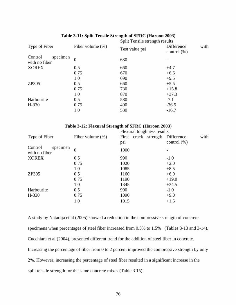
76
Table 3-11: Split Tensile Strength of SFRC (Haroon 2003)
Split Tensile strength results Type of Fiber Fiber volume (%) Test value psi Difference with
control (%) Control specimen with no fiber 0 630 -
0.5 660 +4.7 0.75 670 +6.6
XOREX
1.0 690 +9.5 0.5 660 +5.5 0.75 730 +15.8
ZP305
1.0 870 +37.3 0.5 580 -7.1 0.75 400 -36.5
Harbourite H-330
1.0 530 -16.7
Table 3-12: Flexural Strength of SFRC (Haroon 2003) Flexural toughness results
Type of Fiber Fiber volume (%) First crack strength psi
Difference with control (%)
Control specimen with no fiber 0 1000 -
0.5 990 -1.0 0.75 1020 +2.0
XOREX
1.0 1085 +8.5 0.5 1160 +6.0 0.75 1190 +19.0
ZP305
1.0 1345 +34.5 0.5 990 -1.0 0.75 1090 +9.0
Harbourite H-330
1.0 1015 +1.5 A study by Nataraja et al (2005) showed a reduction in the compressive strength of concrete specimens when percentages of steel fiber increased from 0.5% to 1.5% (Tables 3-13 and 3-14). Cucchiara et al (2004), presented different trend for the addition of steel fiber in concrete. Increasing the percentage of fiber from 0 to 2 percent improved the compressive strength by only 2%. However, increasing the percentage of steel fiber resulted in a significant increase in the split tensile strength for the same concrete mixes (Table 3.15).

77
Table 3-13: Compressive Strength of SFRC FOR 30 MPa Mix (Nataraja et al., 2005)
Table 3-14: : Compressive Strength of SFRC for 50 MPa Mix (Nataraja et al., 2005)
Table 3-15: Compressive and Tensile Strength for SFRC (Cucchiara et al., 2004)
78
CHAPTER 4
ANCHORAGE SPECIMENS SELECTION AND TESTING
4.1 Introduction to Specimen Selection
In this study the dimensions of the tested samples were selected based on preliminary analyses
conducted using finite element modeling (Figure 4-1). Initially, a bridge segment was chosen,
modeled and thoroughly analyzed under post tensioned loading conditions similar to what are
encountered in the field. The purpose this analysis was to define the extent of the post-tensioning
stresses around the anchorage zones in a full scale mode. Such a step was necessary to delineate
the boundary conditions of the anchorage zone if smaller sections were to be considered.
Constitutive properties for finite element modeling including compressive strength, tensile
strength and percentage of fiber contents were selected from a similar study conducted by
Haroon 2003 using the steel fiber proposed for this investigation.
After the full scale analyses of the bridge segment, a scaled block containing two posttensioning
anchors was separated from the web area of the bridge segment. This block was then analyzed
using three dimensional finite element modeling to determine the boundary conditions at which
stress distributions were not affected by the length of the block. For this block, the final
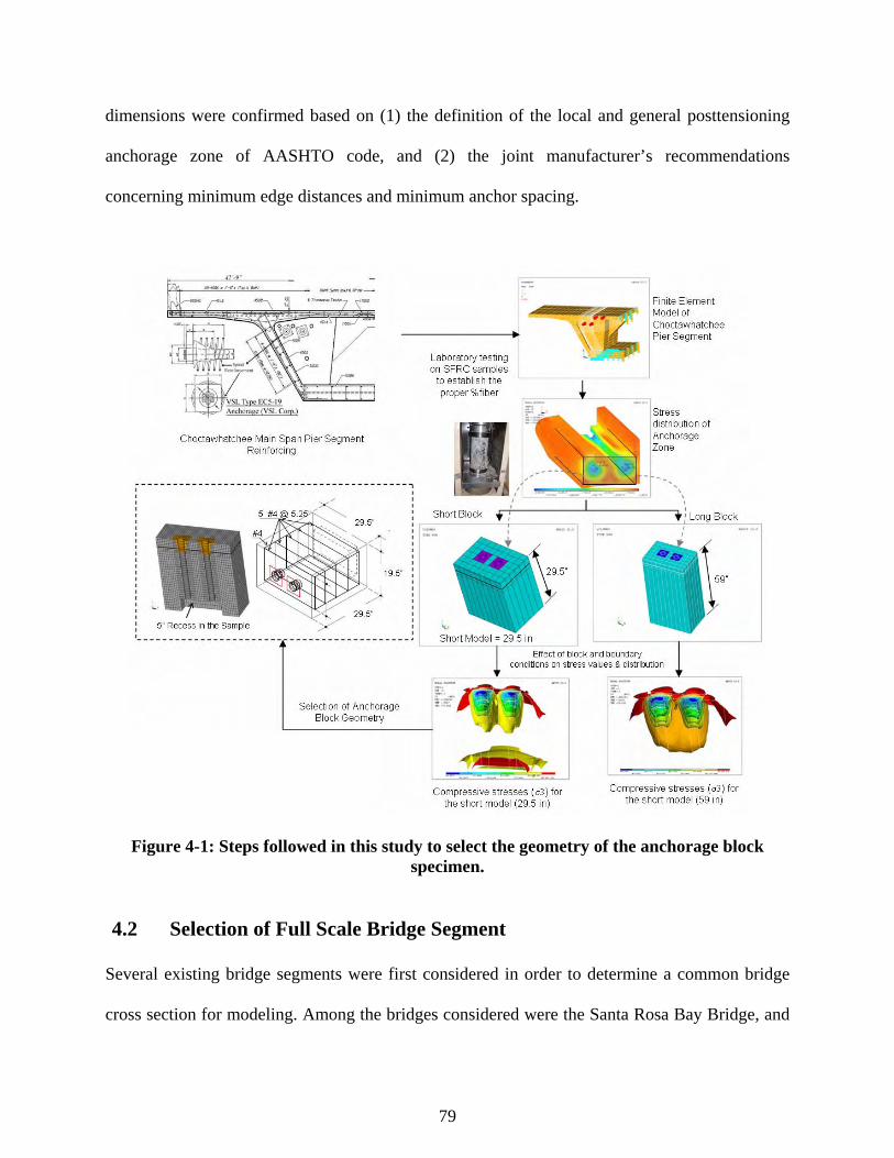
79
dimensions were confirmed based on (1) the definition of the local and general posttensioning
anchorage zone of AASHTO code, and (2) the joint manufacturer’s recommendations
concerning minimum edge distances and minimum anchor spacing.
Figure 4-1: Steps followed in this study to select the geometry of the anchorage block specimen.
4.2 Selection of Full Scale Bridge Segment
Several existing bridge segments were first considered in order to determine a common bridge
cross section for modeling. Among the bridges considered were the Santa Rosa Bay Bridge, and

80
the Choctawhatchee Bay Bridge (Mid-Bay). Both bridges were designed by FIGG Engineering
Group. Further comparison between the two bridge segments revealed that the cross sections
were also fairly similar (Table 4.1). Due to geometry and modeling complexity, the
Choctawhatchee Bay Bridge was chosen to be a representative model and a simplified drawing
can be seen in Figure 4.1.
Table 4-1: Comparison of Bridge Dimensions Project Width Height Length
Santa Rosa Bay Bridge 7’-10” 8’-0” 9’-5”
Choctawhatchee Bay Bridge 8’-1” 9’-0” 9’-5”
Figure 4-2: Choctawhatchee Bay Bridge Segment
The post-tensioning steel required for the bridge was provided in the contract plans of the
Choctawhatchee Bay Bridge. The segment that was chosen detailed two 19-0.6” diameter
longitudinal tendons (Figure 4-2) on each face. VSL type EC 5-19 anchorages were used in
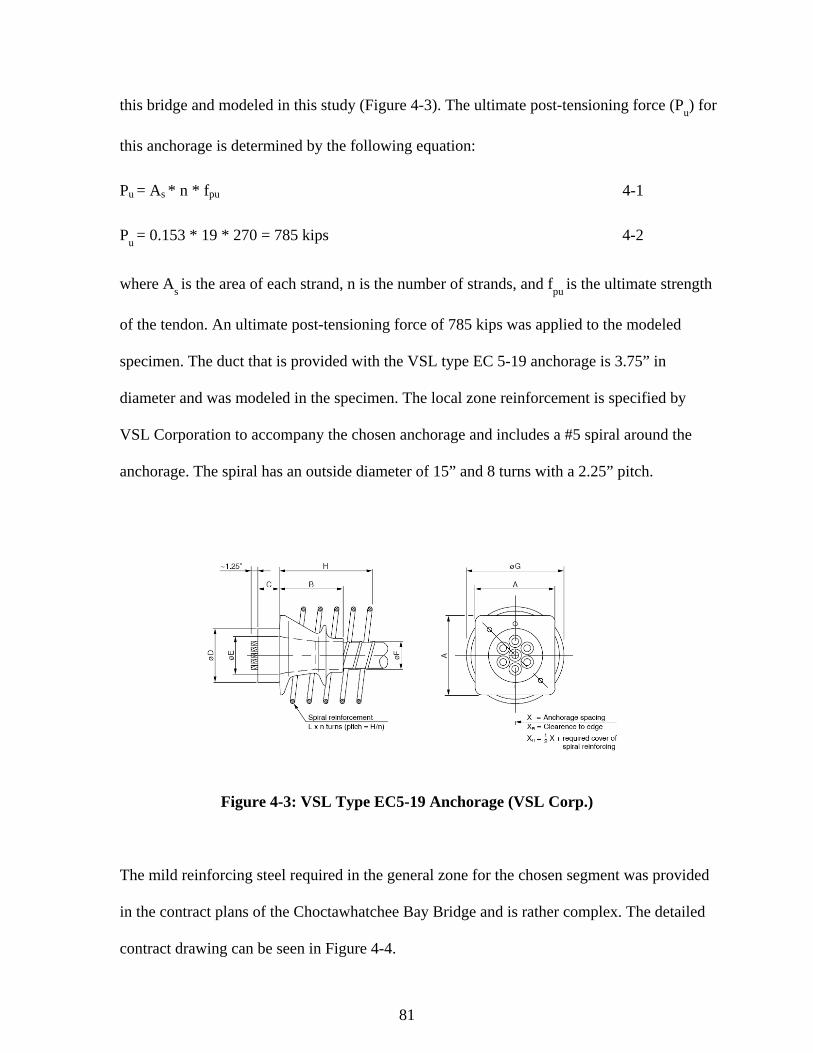
81
this bridge and modeled in this study (Figure 4-3). The ultimate post-tensioning force (Pu) for
this anchorage is determined by the following equation:
Pu = As * n * fpu 4-1
Pu = 0.153 * 19 * 270 = 785 kips 4-2
where As is the area of each strand, n is the number of strands, and fpu is the ultimate strength
of the tendon. An ultimate post-tensioning force of 785 kips was applied to the modeled
specimen. The duct that is provided with the VSL type EC 5-19 anchorage is 3.75” in
diameter and was modeled in the specimen. The local zone reinforcement is specified by
VSL Corporation to accompany the chosen anchorage and includes a #5 spiral around the
anchorage. The spiral has an outside diameter of 15” and 8 turns with a 2.25” pitch.
Figure 4-3: VSL Type EC5-19 Anchorage (VSL Corp.)
The mild reinforcing steel required in the general zone for the chosen segment was provided
in the contract plans of the Choctawhatchee Bay Bridge and is rather complex. The detailed
contract drawing can be seen in Figure 4-4.

82
Figure 4-4: Choctawhatchee Main Span Pier Segment Reinforcing (FIGG)
4.3 Development of the Finite Element Model for Bridge Segment
The first step in developing the 3-D finite element model was to input the geometry of the
segment, including the post-tensioning duct and anchorage, into ANSYS. First, the key
points for the model were defined. Then the lines were drawn between key points to form the
boundaries of the segment and also to break the segment into subunits for meshing purposes.
Lastly, volumes were created based on the areas in the model. Several ways of breaking up
the segment were explored and the optimal segment was taken as seen in Figure 4.5.

83
Figure 4-5: ANSYS Model of Volumes
The optimal designation has to do with the meshing capabilities of the program. A few rules
to follow are given. The mesh should consist of quad (brick) elements; therefore all volumes
must be either four or six sided. Due to the complex geometry of the segment, there were
volumes that had to be five sided. In this situation two sides were chosen to act as one, which
the program calls concatenation. This means that the mesh will flow from one side and
disperse to the two concatenated sides. The mesh should also be fairly consistent. The density
of the mesh should be similar throughout the segment to prevent clusters of nodes from
forming in places with tight geometry. These clusters can cause stress concentrations in the
analysis, raising questions on the validity of the results. The current model has the 463 key
points, 1,155 lines, 914 areas, 230 volumes, and 6,082 solid and shell elements.
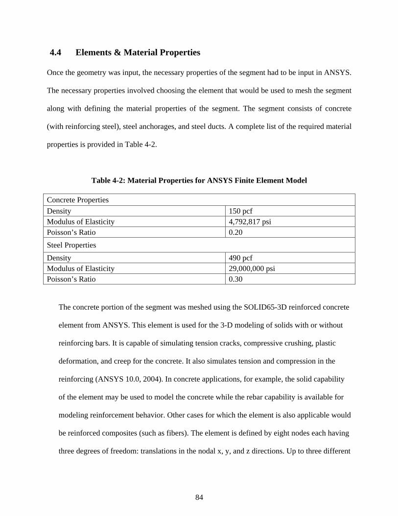
84
4.4 Elements & Material Properties
Once the geometry was input, the necessary properties of the segment had to be input in ANSYS.
The necessary properties involved choosing the element that would be used to mesh the segment
along with defining the material properties of the segment. The segment consists of concrete
(with reinforcing steel), steel anchorages, and steel ducts. A complete list of the required material
properties is provided in Table 4-2.
Table 4-2: Material Properties for ANSYS Finite Element Model
Concrete Properties Density 150 pcf Modulus of Elasticity 4,792,817 psi Poisson’s Ratio 0.20 Steel Properties Density 490 pcf Modulus of Elasticity 29,000,000 psi Poisson’s Ratio 0.30
The concrete portion of the segment was meshed using the SOLID65-3D reinforced concrete
element from ANSYS. This element is used for the 3-D modeling of solids with or without
reinforcing bars. It is capable of simulating tension cracks, compressive crushing, plastic
deformation, and creep for the concrete. It also simulates tension and compression in the
reinforcing (ANSYS 10.0, 2004). In concrete applications, for example, the solid capability
of the element may be used to model the concrete while the rebar capability is available for
modeling reinforcement behavior. Other cases for which the element is also applicable would
be reinforced composites (such as fibers). The element is defined by eight nodes each having
three degrees of freedom: translations in the nodal x, y, and z directions. Up to three different

85
rebar specifications may be defined. The meshed finite element model is shown in Figure
4-6.
Figure 4-6: Segments Modeled for FEM Analysis
Table 4-3 details these segments. As previously mentioned, the compressive and tensile
strengths increase with the addition of steel fiber. The segments had varying amounts of steel
fibers and the design required mild steel reinforcement. The designation of 100% mild
reinforcement is based on the design-required amount and indicates that 100% of what was
required by design was modeled. The purposes of the differing amounts of fiber were to
determine the optimal amount of fiber to add for increased strength. Additional segments
were analyzed with the optimal amount of fiber and decreased mild reinforcement to prove
that the addition of fiber allows a reduction in mild reinforcement.

86
Table 4-3: Segments Modeled Using ANSYS
Finite Element Model No.
Fiber Volume
(% concrete vol.)
Mild Reinforcement (% required)
Compressive Strength (psi)
Tensile Strength (psi)
1 0 100 6,250 625
2 0.25 100 7,112 631
3 0.25 0 7,112 631
4 0.50 100 7,187 655
5 0.50 0 7,187 655
6 0.75 100 7,281 724
7 0.75 0 7,281 724
8 1.0 100 7,393 863
9 1.0 0 7,393 863
4.5 FEM Stress Results & Discussion
Stress results obtained from the FEM are presented and discussed in this section. A
discussion of each analysis along with the reasoning behind the particular analysis follows.
Individual analysis results are presented separately. Finally, a comparison of the analyses is
presented. Segment 1 (Table 4.3) was the control analysis that contained the design required
amount of mild steel reinforcement with no steel fiber reinforcement. This analysis was
performed to provide predicted results to a solution in order to prove the validity of the
model. It also gave a basis for which to compare results of segments with fiber. This segment
was loaded with 1,256 kips of post-tensioning force on each face and the resulting stress
contours at the general zone can be seen in Figures 4.7 through 4.14. Figures 4.7 through 4.9
show the X-, Y-, and Z-component stresses, respectively. Figures 4.10 through 4.12 show the
1st, 2
nd, and 3
rd principal stresses, respectively and Figure 4.13 shows the Von Mises stress

87
contour. These are shown in order to emphasize that all stresses were studied to provide
confidence in the finite element model and results. Out of all of the stresses considered in this
study, the X-component stress is the most important since it reflects the tensile bursting force
in the general anchorage zone. Figure 4-14 shows a plot of the X-component stresses versus
distance across the ducts in the general zone. Table 4-4 details the maximum X-component
stress results in the general zone for segment 1.
Figure 4-7: X-Component Stress (lb/ft2) Contour in Segment 1

88
Figure 4-8: Y-Component Stress (lb/ft2) Contour in Segment 1
Figure 4-9: Z- Component Stress (lb/ft2) Contour in Segment 1
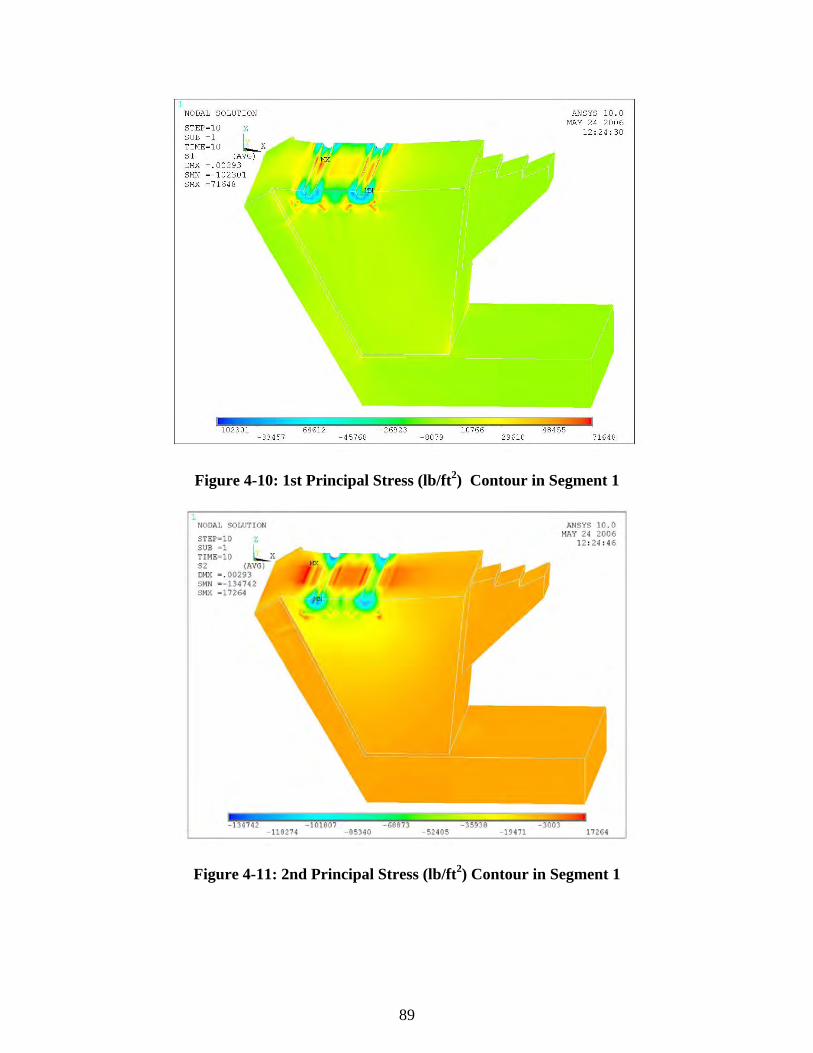
89
Figure 4-10: 1st Principal Stress (lb/ft2) Contour in Segment 1
Figure 4-11: 2nd Principal Stress (lb/ft2) Contour in Segment 1

90
Figure 4-12: 3rd Principal Stress (lb/ft2) Contour in Segment 1
Figure 4-13: Von Mises Stress (lb/ft2) Contour in Segment 1
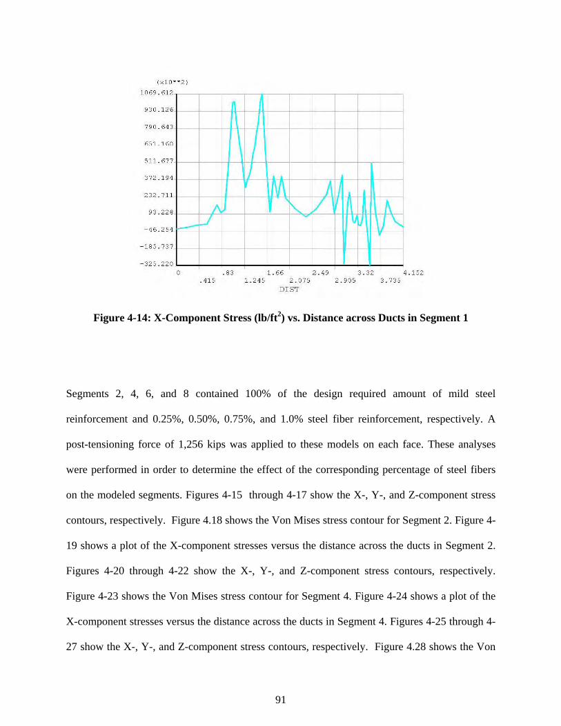
91
Figure 4-14: X-Component Stress (lb/ft2) vs. Distance across Ducts in Segment 1
Segments 2, 4, 6, and 8 contained 100% of the design required amount of mild steel
reinforcement and 0.25%, 0.50%, 0.75%, and 1.0% steel fiber reinforcement, respectively. A
post-tensioning force of 1,256 kips was applied to these models on each face. These analyses
were performed in order to determine the effect of the corresponding percentage of steel fibers
on the modeled segments. Figures 4-15 through 4-17 show the X-, Y-, and Z-component stress
contours, respectively. Figure 4.18 shows the Von Mises stress contour for Segment 2. Figure 4-
19 shows a plot of the X-component stresses versus the distance across the ducts in Segment 2.
Figures 4-20 through 4-22 show the X-, Y-, and Z-component stress contours, respectively.
Figure 4-23 shows the Von Mises stress contour for Segment 4. Figure 4-24 shows a plot of the
X-component stresses versus the distance across the ducts in Segment 4. Figures 4-25 through 4-
27 show the X-, Y-, and Z-component stress contours, respectively. Figure 4.28 shows the Von

92
Mises stress contour for Segment 6. Figure 4-29 shows a plot of the X-component stresses versus
the distance across the ducts in Segment 6. Figures 4-30 through 4-32 show the X-, Y-, and Z-
component stress contours, respectively and Figure 4-33 shows the Von Mises stress contour for
Segment 8. Figure 4-34 shows a plot of the X-component stresses versus the distance across the
ducts in Segment 8. Table 4-4 also details the maximum X-component stresses in the general
zones of segments 2, 4, 6, and 8.
Figure 4-15: X-Component Stress (lb/ft2) Contour in Segment 2

93
Figure 4-16: Y-Component Stress (lb/ft2) Contour in Segment
Figure 4-17: Z-Component Stress (lb/ft2) Contour in Segment 2

94
Figure 4-18: Von Mises Stress (lb/ft2) Contour in Segment 2
Figure 4-19: X-Component Stress (lb/ft2) vs. Distance Across Ducts in Segment 2

95
Figure 4-20: X-Component Stress (lb/ft2) Contour in Segment 4
Figure 4-21: Y-Component Stress (lb/ft2) Contour in Segment 4

96
Figure 4-22: Z-Component Stress (lb/ft2) Contour in Segment 4
Figure 4-23: Von Mises Stress (lb/ft2) Contour in Segment 4

97
Figure 4-24: X-Component Stress(lb/ft2) vs. Distance Across Ducts n Segment 4
Figure 4-25: X-Component Stress (lb/ft2) Contour in Segment 6

98
Figure 4-26: Y-Component Stress (lb/ft2) Contour in Segment 6
Figure 4-27: Z-Component Stress (lb/ft2) Contour in Segment 6

99
Figure 4-28: Von Mises Stress (lb/ft2) Contour in Segment 6
Figure 4-29: X-Component Stress (lb/ft2) vs. Distance across Ducts in Segment 6
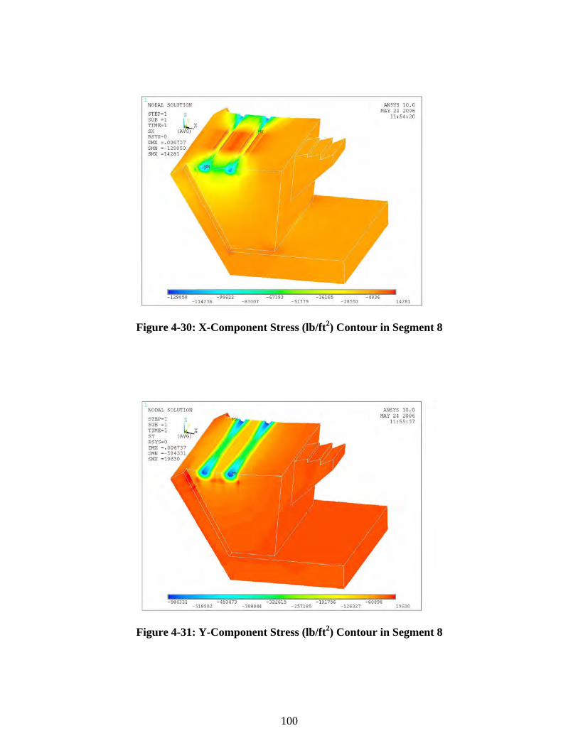
100
Figure 4-30: X-Component Stress (lb/ft2) Contour in Segment 8
Figure 4-31: Y-Component Stress (lb/ft2) Contour in Segment 8

101
Figure 4-32: Z-Component Stress (lb/ft2) Contour in Segment 8
Figure 4-33: Von Mises Stress (lb/ft2) Contour in Segment 8

102
Figure 4-34: X-Component Stress (lb/ft2) vs. Distance across Ducts in Segment 8
Table 4-4: Comparison of Maximum X-Component Stresses
Finite Element Model No.
Fiber Volume (% concrete volume)
Mild Reinforcement (% required)
Max. X-Component Stress (psi)
1 0 100 175.1 2 0.25 100 105.0 4 0.50 100 97.0 6 0.75 100 95.7 8 1.0 100 99.2
Segments 3, 5, 7, and 9 contained no mild steel reinforcement and 0.25%, 0.50%, 0.75%, and
1.0% steel fiber reinforcement, respectively. These analyses were performed in order to study
the behavior of segments that contain only steel fiber reinforcement in the corresponding
amounts. Segments 3 and 5 failed at approximately 40% of the load application in the

103
analyses. This was determined because the finite element model would not produce a
converged solution past the 40% load step. Failure cracking occurred around the ducts and
can be seen in Figures 4-35 and 4-36. Segments 7 and 9 sustained the entire load. However,
severe cracks formed around the ducts similar to those in segments 3 and 5, and can be seen
in Figures 4-37 and 4-38. It may be inferred that mild steel in the general zone cannot be
completely replaced by steel fiber, at least in the amounts studied. Therefore, these cases
were not further investigated herein. See Table 4-5 for failure load results of segments 3, 5, 7,
& 9.
Table 4-5: Failure Load Results
Finite Element Model No.
Fiber Volume (% concrete volume)
Mild Reinforcement (% required)
Failure Load (kips)
3 0.25 0 502.4 5 0.50 0 502.4 7 0.75 0 1256 9 1.00 0 1256

104
Figure 4-35: Cracks in Segment 3 at Failure
Figure 4-36: Cracks in Segment 5 at Failure

105
Figure 4-37: Cracks in Segment 7
Figure 4-38: Cracks in Segment 9

106
Maximum stress versus amount of steel fiber results were plotted for segments 1, 2, 4, 6, and
8 and are shown in Figure 4-39. As expected, the curve shows that stresses decreased with
the addition of steel fiber. From the curve, it can be seen that the greatest stress reduction
occurred when 0.75% steel fibers were added to the concrete. It can also be seen that the
addition of steel fiber in 1.0% amounts actually causes an increase in stresses in the general
zone as compared to the 0.50% and 0.75%. Placement of steel fiber adds dead load to the
segment. This increase in dead load causes an increase in stresses in all directions, since the
steel fibers are placed in all directions. Table 4-6 shows the amount of load that was added to
the general zone with each amount of steel studied. These loads are relatively small in
comparison to the post-tensioning load and the increase in stress is relatively small in
comparison to the lower fiber percentages.
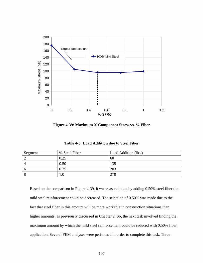
107
0
20
40
60
80
100
120
140
160
180
200
0 0.2 0.4 0.6 0.8 1 1.2% SFRC
100% Mild Steel
Max
imum
Stre
ss (p
si)
Stress Reducation
Figure 4-39: Maximum X-Component Stress vs. % Fiber
Table 4-6: Load Addition due to Steel Fiber
Segment % Steel Fiber Load Addition (lbs.) 2 0.25 68 4 0.50 135 6 0.75 203 8 1.0 270
Based on the comparison in Figure 4-39, it was reasoned that by adding 0.50% steel fiber the
mild steel reinforcement could be decreased. The selection of 0.50% was made due to the
fact that steel fiber in this amount will be more workable in construction situations than
higher amounts, as previously discussed in Chapter 2. So, the next task involved finding the
maximum amount by which the mild steel reinforcement could be reduced with 0.50% fiber
application. Several FEM analyses were performed in order to complete this task. Three

108
additional segments were loaded with 1256 kips and studied. Table 4-7 shows results for
steel amounts and X-component stress values in comparison to the control analysis.
Table 4-7: Comparison of Additional Segments
Segment Fiber Volume (% concrete volume)
Mild Reinforcement (% required)
Max. X-Component Stress (psi)
1 0 100 175.1 10 0.50 50 129.3 11 0.50 45 143.1 12 0.50 44 Failure
Segment 10 contained 0.50% steel fiber and 50% design required mild steel reinforcement.
Figure 4-40 shows the X-component stress contour of segment 10 at the general zone. Figure
4-41 shows a plot of X-component stresses versus distance across the ducts. The resulting
maximum X-component stress was lower than the control analysis; so further reduction of
the mild steel reinforcement was possible. Segment 11 contained 0.50% steel fiber and 45%
design required mild steel. Figure 4-42 shows the X-component stress contour of segment 11
at the general zone. Figure 4-43 shows a plot of X-component stresses versus distance across
the ducts. The maximum stress was still lower than the control analysis. In a final attempt to
determine the maximum reduction, segment 12 was analyzed with 0.50% steel fiber and 44%
mild steel reinforcement. The segment failed at 70% load application, or at approximately
879 kips. The cracking around the ducts was similar to segments 7 and 9 and is presented in
Figure 4-44. The geometry of the block that contains the general stress zone in the segment
is shown in Figure 4-45.

109
Figure 4-40: X-Component Stress (lb/ft2) Contour in Segment 10
Figure 4-41: X-Component Stress (lb/ft2) vs. Distance Across Ducts in Segment 10

110
Figure 4-42: X-Component Stress (lb/ft2) Contour in Segment 11
Figure 4-43: X-Component Stresses (lb/ft2) vs. Distance across Ducts in Segment 11

111
Figure 4-44: Crack distribution at Failure (red circles) in Segment 12
Figure 4-45: Stresses in General Zone

112
The maximum permissible reduction of mild steel reinforcement with the addition of 0.50% steel
fiber was 55% in the general zone. However, the segment failed with a 56% reduction.
Therefore, reducing the mild steel reinforcement in the general zone by 55% is not
recommended. The optimal reduction would occur at 50% in order to be conservative and safe.
As previously mentioned, the addition of the steel fiber added self weight of the segment. It is
reasonable to consider that the increased self weight would also impact other areas of the
segment. Figure 4-46 shows the overall stress contour of segment 8, which contained 1.0% steel
fiber and 100% mild steel reinforcement. Some stress concentrations could be seen at the top
slab of the segment near the web-flange connection and at the unsupported portion of the top slab
of the segment near the diaphragm (where the plates are located).
Figure 4-46: Overall Stress (lb/ft2) Contour for Segment 8

113
4.6 AASHTO Requirements for General Zone Size
Section 5.10.9.6.1 of the AASHTO code lists conditions that must be true for stresses and forces
to be estimated using the approximate stress analyses and design equations. One of the
conditions stated in AASHTO Section 5.10.9.6.1 is that “the minimum edge distance of the
anchorage in the main plane of the member is not less than 1.5 times the corresponding lateral
dimension, a, of the anchorage device.” Since the research team believed consideration should
be given to the stresses that will develop between the two anchorage devices, the size of the
anchorage test specimen was based upon the use of two (2) VSL EC 5-7 anchorage devices
embedded in each specimen.
By considering the conditions necessary for use of the approximate analysis method, calculations
were made to help determine the anchorage test specimen size needed to meet the conditions.
The calculated values are shown Table 4-8 to Table 4-14. An examination of these tables will
show that several different parameters were considered in determining the size of the anchorage
test specimen. These parameters included number, of PT anchorages, size of PT anchorages, and
concrete cover. From Table 4-8 to Table 4-9, it can be seen that for using two (2) VSL anchors,
the minimum specimen dimensions are X = 29.03”, Y = 19.5” and Z = 29.03”. Therefore, the
anchorage test specimen was chosen to be 29.5” x 19.5” x 29.5” (or 19.5” x 29.5” x 29.5”
depending upon the orientation of the specimen). The bearing surface for the anchorages was
selected to be 19.5” x 29.5”. The length of the specimen (parallel to the tendon path) was
selected to be 29.5”. As shown in the other tables, values were computed for the approximate
bursting force, bursting steel, etc. However, these values were based upon using the design force

114
for the tendons, a total tendon force of 520.2 Kips (1.2 x the tendon jacking force) for the two
tendons. For this load, Tburst and dburst were computed as 64.86 Kips and 14.52”, respectively.
Maximum load values from the load tests were used to compute Tburst and dburst based upon the
approximate stress analysis method and the equations given in Section 5.10.9.6.3 of the
AASHTO code. These computed values are shown in Table 4-15 for the block specimens which
will be used in the laboratory testing program. The geometric dimensions of the PT test
specimens and a photograph of one test specimen are shown in Figure 4-47 and Figure 4-48.
The laboratory testing program is presented in Chapter 5.
Table 4-8: Stress Analysis Used To Size Anchorage Test Specimen, Part 1

115
Table 4-9: Stress Analysis Used To Size Anchorage Test Specimen, Part 2
Table 4-10: Stress Analysis Used To Size Anchorage Test Specimen, Part 3
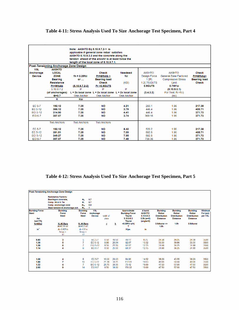
116
Table 4-11: Stress Analysis Used To Size Anchorage Test Specimen, Part 4
Table 4-12: Stress Analysis Used To Size Anchorage Test Specimen, Part 5

117
Table 4-13: Stress Analysis Used To Size Anchorage Test Specimen, Part 6
Table 4-14: Stress Analysis Used To Size Anchorage Test Specimen, Part 7

118
Table 4-15: Approximate Stress Analysis For S1 and S2 Specimens
Figure 4-47: Dimensions of the PT Anchorage Specimen

119
Figure 4-48: Block Specimens during Construction Showing Internal Instrumentation

120
CHAPTER 5
LABORATORY TESTING OF BLOCK SPECIMENS
5.1 Post-Tensioning Anchorages and Ducts
Two of the major post-tensioning anchorage system suppliers in the United States are VSL
Corporation and Dywidag Systems International. Two (2) different post-tensioning anchorage
systems (one supplied by each of the two manufacturers) were used in this test program. The
size of the post-tensioning anchors was limited based upon consideration of the 1000K load
capacity of the FDOT load testing frame. Thus, based upon the size of the test specimen and the
use of two (2) anchors in each specimen, a relatively small anchor system (with design capacity
of 289K) was used. The PT test specimen size was selected with the intent of ensuring that most
of the specimens would fail under loading prior to reaching the load capacity of the FDOT 1,000
kips loading frame.
5.2 VSL EC 5-7 Post-Tensioning Anchorages and Ducts
The VSL anchor designation for the 289Kips capacity PT anchor is VSL Type EC 5-7. Figure
5-1 shows the geometry of the EC 5-7 anchor. In addition to PT anchors, post-tensioning ducts
and spirals were embedded in the test specimens. The duct used is a plastic duct.

121
Figure 5-1: VSL EC 5-7 Post-Tensioning Anchor
5.3 Dywidag MA 5-0.6 Post-Tensioning Anchorages and Ducts
The Dywidag anchor designation for the 289K capacity PT anchor is Dywidag MA 5-0.6.
Figure 5-2 gives the dimensions for the anchor. In addition to PT anchors, the post-tensioning
ducts were also used in the test specimens. The duct used is a 59 mm plastic duct.

122
Figure 5-2: Dywidag MA 5-0.6 Post-Tensioning Anchor
5.4 Non-Prestressed Steel Reinforcement
The AASHTO code divides the post-tensioning (PT) anchorage zone into two sections, the local
zone and the general zone. In accordance with the AASHTO code, the anchorage device
supplier is responsible for providing anchorage devices and records of acceptance tests which
comply with the AASHTO requirements. In addition, the anchorage device supplier “shall
specify auxiliary and confining reinforcement, minimum edge distance, minimum anchor
spacing, and minimum concrete strength at time of stressing required for proper performance of
the local zone (AASHTO, 2007)”. The local zone includes the anchor system and the
surrounding concrete. To help prevent failure of the anchor system, for both the VSL and the

123
Dywidag anchors, the anchorage device design includes a steel spiral which is to be installed
with the anchors. Thus, the spiral size and geometry are specified for each anchor. In the
general zone, bursting steel is provided to prevent excessive cracking due to the bursting stresses
that develop in the concrete. For PT test specimens, the bursting steel design is based upon the
equations given in Sections 5.9 and 5.10 of the AASHTO LRFD Bridge Design Specifications
(2007).
5.4.1 Spiral Reinforcement for VSL Anchors
As shown in the VSL Type E anchor table, Figure 5-1, the spiral to be used with the VSL EC 5-7
anchor was # 4 bar spiral with a diameter of 9.0 inches and 6 turns. Twelve inches (12”) is the
distance that the spiral shall extend beyond the outer surface of the PT anchor into the PT anchor
zone. Using this information, the computed pitch for the spiral is 2” (Figure 5-3).
Figure 5-3: Anchors used in the Study

124
5.4.2 Spiral Reinforcement for Dywidag Anchors
As shown in the Dywidag Multi-plane Anchorage MA table, Figure 5-2, the spiral used with the
MA 5-0.6 anchor was # 4 bar with a diameter of 7.75 inches. Ten inches (10”) is the distance that
the spiral shall extend beyond the outer surface of the PT anchor into the anchor zone. The pitch
for the spiral is 1.875”.
5.4.3 Tie Reinforcement for VSL and Dywidag Anchors
The tie reinforcement used for the anchor test specimens was determined by considering the
2004 AASHTO code, Section 5.10.9.6.3 and Section 5.10.10.1 for post-tensioned anchorage
zone design using “Approximate Stress Analysis”. For the VSL EC 5-7 anchor with a
Guaranteed Ultimate Tensile Strength (GUTS) of 289 K, the approximate bursting force, Tburst
was computed to be 48.2 K. The distance used to determine the distribution distance for the
bursting steel, dburst, was computed to be 9.75”. In accordance with AASHTO Section 5.10.9.6.3
the bursting rebar should be distributed for a distance of 2.5(dburst) but less than or equal to a
distance of 1.5h, where h equals 19.5” for the anchorage specimen using two (2) EC5-7 anchors.
Tie reinforcement was provided to satisfy the AASHTO recommendation by using five (5) # 4
bars spaced at 5.25” (Figure 5-4). However, in the test specimen matrix, in order to consider the
effect of reducing the amount of bursting steel in favor of adding steel fiber, some specimens
were cast with only three (3), # 4 bars spaced at 10.5 inches.

125
Figure 5-4: Anchorage Test Specimen Steel Tie Reinforcement.
5.5 Fibers and Fiber Percentages Used In Anchorage Test Specimens
The three (3) fibers used in the research project are Dramix ZP305, Helix, and Novomesh 850.
Dramix ZP305 (a steel fiber) was used in earlier tests conducted for the Florida Department of
Transportation (FDOT) by Yazdani, et al (2002) and Haroon (2003). The Dramix, Helix and
Novomesh fibers are shown in Figure 3-1. PT anchorages test specimens were cast using each of
the three fibers.
5.6 Anchorage Specimens
In an effort to consider the effects of several variables (type of steel fiber, confinement steel,
bursting steel and anchorage device), twenty-seven (27) test specimens were cast with embedded
post-tensioning anchors and ducts. Twenty-three (23) of the specimens were cast with steel
fibers and four (4) were cast with plain concrete.

126
5.7 Concrete Used for Anchorage Test Specimens
As presented in Chapter 3, the concrete mix design selected for use in this project is a 4000 psi
mix recommended by the FDOT Materials Lab. A mix with a relatively high slump was used
since the addition of steel fibers was expected to reduce the concrete slump. Table 3-1 shows the
concrete mix design for the 4000 psi which is the minimum concrete strength recommended for
post-tensioned anchorage.
A total of 8 batches of concrete were cast to make the twenty-seven (27) test specimens:
Thirteen (13) specimens (S1 Specimens) were cast with VSL PT anchors. Fourteen (14)
specimens (S2 Specimens) were cast with Dywidag PT anchors. Table 3-3 and Table 3-9 show
the mix proportions of the four concrete batches used to cast S1 Specimens. The four concrete
batches used to cast the S2 Specimens are shown in Table 3-9. Based upon the preliminary
material test results (which were presented in Chapter 3) and the finite element modeling
(Chapter 4), the fiber percentage used for the test specimens was 0.5% for each of the three
fibers.
From each concrete batch, concrete cylinders were cast and tested to obtain material properties
for the anchorage test specimens. From these cylinders, compressive strength tests and split
tensile strength tests were performed. The test results were presented earlier (Figure 3-2 to
Figure 3.7). For S1 Specimens, The average 28 day compressive strengths for Plain, Dramix,
Helix and Novomesh cylinders were 4846 psi, 4767 psi , 2848 psi, and 4305 psi, respectively.

127
For S1 Specimens, the average 28 day split tensile strengths for Plain, Dramix, Helix and
Novomesh cylinders were 362 psi, 427 psi, 389 psi and 408 psi, respectively.
5.8 Instrumentation and Data Acquisition Equipment
This section provides information about the instrumentation and data acquisition system used in
the test program. Internal instrumentation, strain gages were purchased from Vishay
Micromeasurements. All external gages and the data acquisition system were supplied by the
Florida Department of Transportation’s Structures Research Center.
5.8.1 Instrumentation of Anchorage Test Specimens
During the test, both strains and displacements were measured and recorded. Internal and
external strain gages were used. The internal gages were mainly 5” gages by Vishay
Micromeasurements (models EPG-5-350W and EPG-5-120W). The external (surface) gages
were TML Model PL-60-11, 60 mm, 120 ohm, foil strain gages. Displacements of the test
specimens were measured using a TML Model SDP-2000, full bridge, displacement transducers
and Balluf Model BOD 66M Class II Laser distance measurement sensors. Instrument locations
for internal gages are as indicated in Figure 5-5 and Figure 5-6. Installation of internal gages is
shown in Figure 5-7.

128
Figure 5-5: Instrumentation of Block Specimen
Figure 5-6: Block Specimen Instrumentation

129
Figure 5-7: Installation of Embedded Gauges
5.8.2 Data Acquisition System
The test data was sampled and recorded using a data acquisition system manufactured by
National Instruments: Chassis Model PXI-1011 combo PXI/SCXI, Controller Model PXI-8176
embedded controller running Windows XP/LabView, DAC (ADC) Card Model PXI-6251,
Signal Conditioning Model SCXI-1530 strain gage module. With this data acquisition system,
the data was sampled at 1 kHz, averaging every 100 samples for a recording rate of 10 Hz.
During testing the target strain rate was three (3) microstrains per second.

130
5.9 Testing Setup
The PT anchor test specimens were load tested at the Florida Department of Transportation’s
Structures Research Center in Tallahassee, Florida. Photographs of the test setup is shown in
Figure 5-8. As shown in the figure, the 1000 Kip load frame (RSFrame) provided resistance for
two (2) 800 Kips Enerpac actuators (Model #RR-40018). The load of each actuator was
measured by an Interface 600 Kips load cell (Model #1260CHG-600K). The loads were applied
to a heavy steel box which transferred the load to two (2) round steel tendon wedge anchor plates
which loaded the anchors of the test specimen. For the first specimen tested, S1-1, the concrete
test specimen rested on a neoprene bearing pad. For all other tests, the specimens rested in a box
of sand.
Figure 5-8: Test Set up used in the Study

131
5.10 Testing Procedure
Once a test specimen was properly positioned, instrumented and connected to the data
acquisition system, the load was applied to the specimen. Using manual controls, the equipment
operator controlled the load rate and relative magnitude of the load being applied by each
Enerpac actuator. The target load range was three (3) microstrains per second. In general, the
load was applied continuously to a test specimen until the specimen either failed or the capacity
of the load frame was reached. In a few instances, based upon the behavior of the specimen (i.e.
cracking) the load was held steady for a brief period. However, due to the high capacity of the
applied loads, the specimens were observed from a distance until the load cycles were
completed. After the end of a load test, the tested specimen was examined closely. Cracks were
noted and the specimen was photographed. During and after testing, any notable information
was recorded (i.e. load at first cracking, failure mechanism). In the following sections the load
test results for the twenty-seven (27) anchorage test specimens are presented and discussed.
5.11 Anchorage Test Specimens with VSL Anchors (S1)
The bearing surface (bottom surface) of the first test specimen, Specimen S1-1, rested on a
neoprene bearing pad. This pad was larger on all sides than the specimen and was approximately
5” thick. The pad was not new. It was a salvaged bridge bearing pad which was being stored at
the FDOT lab. During testing, Specimen S1-1 experienced differential settlement at the bottom.
This contributed to spalling originating on the east side (one of the narrow sides) of the
specimen. To improve bearing conditions for the next tested specimen, S1-2, the bearing end
rested in a wooden sandbox. Based upon the performance of Specimen S1-2 during the load
test, using the sandbox was considered an improvement. Therefore, all other S1 and S2

132
specimens were tested with the sandbox at bearing surface. In the load testing program, each
specimen was loaded until 1) it failed suddenly due to punching shear or bursting tension, 2) it
failed to carry additional load, or 3) the capacity of the load frame was reached.
Each of the S1 Specimens was cast with two (2) EC5-7 VSL anchors, and each anchor was
designed for a tendon with at Guaranteed Ultimate Tensile Strength (GUTS) of 289 kips. This is
the minimum breaking load for a tendon made of seven (7), 0.5”, 270 ksi low relaxation strands.
Thus, for two anchors the GUTS is 578 kips. For design purposes, VSL literature allows a
temporary overstressing to 80% of the GUTS for the anchor. This load, 80% of GUTS, is 231.2
kips for each anchor. For each test specimen, 80% of GUTS for two anchors is 462.4 kips.
The AASHTO code, Section 5.10.9.7.2 limits the factored bearing resistance of the anchorage to
be Pr = F f’n Ab where fn is the lesser of fn = 0.7f’ci S (A/Ag) and fn = 2.25 f’ci . In the equation
for Pr, Ab is the effective area of the bearing plate. If f’ci, the specified compressive strength of
concrete at the time of initial loading or prestressing, is 3,500 psi (the minimum concrete
compressive strength required for applying maximum prestress force to the anchor), and fn =
2.25f’ci, then for the VSL EC 5-7 anchor, Pr would be calculated as approximately 222 kips for
each anchor. Thus for two anchors, the total bearing resistance would be approximately 444
kips.
By considering 80% of GUTS and the limiting bearing resistance computed above for each
anchor, a total applied load in excess of 444 kips applied to a S1 test specimen would be a load
that approximately exceeds the design capacity of the VSL anchors based on the assumed design

133
parameters. For load testing purposes, if a specimen successfully resists 462.4 kips, the
specimen has fulfilled load capacity requirements for the VSL EC5-7 anchor system.
5.11.1 Anchorage Test Specimen S1-1
Specimen S1-1 was the first one load tested at the FDOT Structures Lab. This specimen
contained plain concrete, two (2) VSL EC5-7 anchors & ducts, a steel spiral and steel ties.
Specimen S1-1 was tested at the age of 138 days. The 28 day compressive strength and the
ninety-six (96) day compressive strength were 4846 psi and 6618 psi, respectively. The 28 day
tensile strength and the ninety-five (95) day tensile strength were 362 psi and 457 psi,
respectively. The first visible surface crack occurred at a load in excess of 400 K. The failure
load of 627.92 Kips was approximately 9% greater than twice the GUTS for one VSL anchor
(2x289K = 578 K).
During the load test it was evident that differential settlement was taking place. At the bottom
of the test specimen on the east side the concrete started to spall before other signs of
deterioration were evident. Failure was initiated by excessive crushing and cracking at the
bottom of the specimen, particularly on the east side. At the highest applied load (627.9 Kips),
the northeast corner of the specimen sheared off. Figure 5-9 shows a network of cracked
developed on the top surface. The development of the cracks can be attributed to the presence of
the bursting reinforcement (#4 bar ties spaced at 5.25”) and the spirals in the local zone. Figure
5-10 to Figure 1-1Figure 5-11 show deflection and strain data from the surface and embedded
gages for Specimen S1-1.

134
Figure 5-9: Crack Patterns for S1 Block (Spirals + Ties)
0
100
200
300
400
500
600
700
800
900
1000
0.0E+00 1.0E-01 2.0E-01 3.0E-01 4.0E-01 5.0E-01 6.0E-01 7.0E-01 8.0E-01 9.0E-01
Deflection (in )
Load
(Kip
s)
S1-1 (Ties & Spirals)
627.917 Kips
Edge Failure
Figure 5-10: Applied Load vs. Deflection for S1 Block (Spirals + Ties).

135
Top Surface Strains (None/Y/Y)
0
100
200
300
400
500
600
700
800
900
1000
-500-300-100100300500
Strain (microstrain)
Tota
l Loa
d (K
ips)
S_Top_SG N_Top_SG
Crack approaching the N_Top_SG
Figure 5-11: Range of Compressive and Tensile Stains at the Top Gauges
5.11.2 Anchorage Test Specimen S1-13
Specimen S1-13 contained plain concrete two (2) VSL EC5-7 anchors, two ducts, approximate
50% of the steel spiral recommended by VSL for the local zone and 60% of the steel ties used in
Specimen S1-1. For this Specimen, the spacing of the steel ties was twice the tie spacing used in
Specimens S1-1. At the bearing end of the specimen, the specimen rested in a wooden sandbox.
S1-13 was tested at an age of 155 days. Cracks developed on all surfaces of Specimen S1-13
during testing. These cracks are show in Figure 5-14 to 5-15. After the load was removed and
the Specimen’s bottom was exposed, it was noted that the bottom surface was greatly
deteriorated with large concrete spalls and cracks. On a portion of the bottom of the specimen,
the bottom layer of the tie reinforcement was exposed.

136
Specimen S1-13 was loaded until failure; a total load of 732.53 Kips was reached. From
looking at the bottom surface of the Specimen it seems that structural integrity of the specimen
was exceeded prior to the application of the final load. However, the specimen was loaded until
it failed to carry additional load since the deteriorated condition of the bottom was not evident
until after the load test was concluded. Similar to S1 block, punching shear did not occur at the
anchors. With a 50% reduction in steel spirals and a 40% reduction in steel ties, Specimen S1-
13 accepted 17% more load than Specimens S1-1. Figure 5-12 to Figure 5-13 show plots of load
vs. deflection and load vs. stain measurements, respectively.
0
100
200
300
400
500
600
700
800
900
1000
0 0.1 0.2 0.3 0.4 0.5 0.6 0.7 0.8 0.9 1
Deflection (in)
Load
(Kip
s)
S1-13- (None/0.5/0.6)
Crack development
Crack propagationaround the anchors
Figure 5-12: Load vs. Deflection of S1-13.

137
Top Surface Strains
0
100
200
300
400
500
600
700
800
900
1000
-600 -400 -200 0 200 400 600
Strain (microstrain)
Tota
l Loa
d (K
ips)
S_Top_SG
N_Top_SG
N Top SG
Figure 5-13: Load vs. Strain Relationship for Embedded Gauges in S1-13.
Figure 5-14: Crack Pattern at the Top Surface of S1-13.

138
Figure 5-15: Crack Pattern at the Bottom Surface of S1-13.
5.11.3 Anchorage Test Specimen S1-2
Specimen S1-2 contained concrete with 0.5% Dramix ZP305 fibers by volume, two (2) VSL
EC5-7 anchors and ducts. The specimen did not contain spirals and ties. At the bearing end of
the specimen, the specimen rested in a wooden sandbox. This was considered an improvement
over using the neoprene bearing pad. Therefore, all other specimens were tested with the
sandbox at bearing surface.
Specimen S1-2 was tested at the age of 153 days. The 28 day compressive strength and the
ninety-six (96) day compressive strength were 4767 psi and 5748 psi, respectively. The 28 day
tensile strength and the ninety-six (96) day tensile strength were 408 psi and 359 psi,
respectively. The failure load of 794 Kips was approximately 137% greater than twice the
GUTS for each VSL anchor (2x289Kips = 578 Kips) (Figure 5-16). Although both the
compressive strength and the tensile strength of the concrete in Specimen S1-2 was less than that
for Specimen S1-1, the failure load of Specimen S1-2 was 26% greater than the failure load for

139
S1-1. The differential settlement of S1-1 may have been the reason for early failure of S1-1.
Strain measurements from embedded gauges show the sudden punching failure for these types of
block specimens Figure 5-17.
0
100
200
300
400
500
600
700
800
900
1000
0 0.1 0.2 0.3 0.4 0.5 0.6 0.7 0.8 0.9 1
Defelction (in)
App
lied
Load
(Kip
s)
S1-2 (Dramix/N/N)
Punching Shear Failure
Figure 5-16: Load vs. Deflection of S1-2.
Embedded Gauges (Dramix/N/N)
0
100
200
300
400
500
600
700
800
900
1000
-600 -400 -200 0 200 400 600 800 1000
Strain (%)
Tota
l Loa
d (K
ips)
EMB_0523_47
EMB_0523_44
Sudden Increase inTensile StressesIndicating Development of Cracks at EMB-0523-44
Figure 5-17: Load vs. Strain Relationship for Embedded Gauges in S1-2.

140
At failure, a major tension (bursting) crack developed on both the east and west faces (on the
19.5’’ sides) of the specimen (Figure 5-19). Steel ties were not present to resist the tensile
forces. Figure 5-19 to Figure 5-20 show the specimen split into two halves. The major break
through the specimen was not accompanied by a network of many small cracks as was the case
in Specimen S1-1. Few other cracks developed on the surfaces. This indicates that the steel
fibers were effective in reducing tension cracks in the surface even though no steel spirals or tie
reinforcement were present. The failure due to punching of the anchors and development of the
large splitting crack on the short sides was sudden and accompanied with a loud explosive sound.
Another major crack was noticed along the lower part of the block indicating bursting stresses
due to the strut and tie action in the general stress zone.
Figure 5-18: Crack Pattern on the Top of S1-2; Typical for all Specimens without Ties.

141
Figure 5-19: Punching Shear Failure of the Anchors in S1-2.
Figure 5-20: Zone of Bursting Cracks Between the two Ducts in S1-2.

142
5.11.4 Anchorage Test Specimen S1-3
Specimen S1-3 contained concrete with 0.5% Dramix ZP305 fibers by volume, two (2) VSL
EC5-7 anchors, two ducts, and steel spirals. The specimen did not contain steel ties. Using the
typical load set-up (the same as used for Specimen S1-2), Specimen S1-3 was loaded until it
failed at a total load of 865.48K (Figure 5-21). Figure 5-22 shows the magnitudes of strain
measurements of embedded gauges.
Specimen 1-3 was tested at the age of 154 days. Specimens S1-2 through S1-5 were all cast
from the same batch of concrete. Thus, the 96 day compressive strength and the 96 day tensile
strength were 5748 psi and 359 psi, respectively. The failure load of this specimen was 9%
higher than the failure load of Specimen S1-2. Thus, test results indicated that the presence of
spirals in the local zone contributed to a 9% increase in load capacity.
0
100
200
300
400
500
600
700
800
900
1000
0 0.1 0.2 0.3 0.4 0.5 0.6 0.7 0.8 0.9 1Defelction (in)
App
lied
Load
(Kip
s)
S1-3 (Dramix/Y/N)
Punching Shear Failure
Figure 5-21: Load vs. Deflection of S1-3.

143
Embedded Gauges (Dramix/Y/N)
0
100
200
300
400
500
600
700
800
900
1000
-800 -600 -400 -200 0 200 400 600 800
Strain (%)
Tota
l Loa
d (K
ips)
EMB_0523-57EMB_0523-49EMB_0523-48
Figure 5-22: Load vs. Strain Relationship for Embedded Gauges in S1-3.
At failure, a major tension (bursting) crack developed on both the east and west faces (on the
19.5’’ sides) of the specimen (Figure 5-23). The major break through the specimen was not
accompanied by a networks of many small cracked as was the case in Specimen S1-1. Few other
cracks developed on the surfaces (Figure 5-24). This indicates that the steel fibers were effective
in reducing tension cracks in the surface even though no steel tie reinforcement was present.
Although, the failure was relatively sudden without a good network of cracks developing, Unlike
S1-2, the punching failure in S1-3 was for the block of steel anchors and the spirals. Two
distinct blocks were resulted from the failure of this specimen as shown in Figure 5-24.
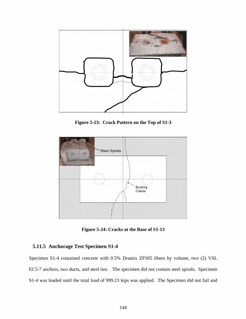
144
Figure 5-23: Crack Pattern on the Top of S1-3
Figure 5-24: Cracks at the Base of S1-13
5.11.5 Anchorage Test Specimen S1-4
Specimen S1-4 contained concrete with 0.5% Dramix ZP305 fibers by volume, two (2) VSL
EC5-7 anchors, two ducts, and steel ties. The specimen did not contain steel spirals. Specimen
S1-4 was loaded until the total load of 999.23 kips was applied. The Specimen did not fail and
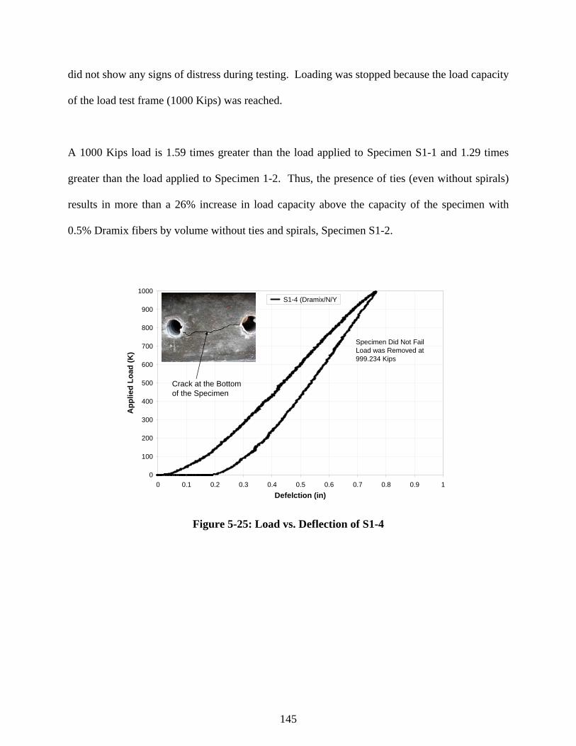
145
did not show any signs of distress during testing. Loading was stopped because the load capacity
of the load test frame (1000 Kips) was reached.
A 1000 Kips load is 1.59 times greater than the load applied to Specimen S1-1 and 1.29 times
greater than the load applied to Specimen 1-2. Thus, the presence of ties (even without spirals)
results in more than a 26% increase in load capacity above the capacity of the specimen with
0.5% Dramix fibers by volume without ties and spirals, Specimen S1-2.
0
100
200
300
400
500
600
700
800
900
1000
0 0.1 0.2 0.3 0.4 0.5 0.6 0.7 0.8 0.9 1Defelction (in)
App
lied
Load
(K)
S1-4 (Dramix/N/Y
Specimen Did Not FailLoad was Removed at 999.234 Kips
Crack at the Bottom of the Specimen
Figure 5-25: Load vs. Deflection of S1-4

146
Embedded Gauges (Dramix/Y/N)
0
100
200
300
400
500
600
700
800
900
1000
-1000 -800 -600 -400 -200 0 200 400 600 800 1000
Strain (microstrain)
Tota
l Loa
d (K
ips)
EMB_0500-38EMB_0523-46EMB_0523-53EMB_0523-33
Figure 5-26: Load vs. Strain Relationship for Embedded Gauges of S1-4.
5.11.6 Anchorage Test Specimen S1-5
Specimen S1-5 contained concrete with 0.5% Dramix ZP305 fibers by volume, two (2) VSL
EC5-7 anchors, two ducts, approximate 50% of the steel spiral recommended by VSL for the
local zone and 60% of the steel ties used in Specimen S1-1. For this specimen, the spacing of
the steel ties was twice the spacing used in Specimens S1-1 and S1-3. Specimen S1-5 was
loaded until a total load of 1000.36 Kips was reached Figure 5-27. The load test was stopped
because the capacity of the load frame was reached.

147
0
100
200
300
400
500
600
700
800
900
1000
0 0.1 0.2 0.3 0.4 0.5 0.6 0.7 0.8 0.9 1Defelction (in)
App
lied
Load
(K)
S1-5 (Dramix/0.5/0.6)
Specimen Did Not FailLoad was Removed at 1,000 Kips
Top Cracks
Bottom Cracks
Figure 5-27: Load vs. Deflection of S1-5.
Cracks developed on the top surface, the east face and the bottom surface of Specimen S1-5
during testing. These cracks are shown in Figure 5-27 and Figure 5-28. The development of
more cracks on the surface than developed for Specimen S1-4 can be attributed to the doubled tie
spacing used in Specimen S1-5. Based upon the strain gage data it is estimated that the first
cracks did not develop until after an applied load of approximately 850 Kips was reached (Figure
5-28).

148
387.5 ( μ strain)
0
100
200
300
400
500
600
700
800
900
1000
1100
-1000 -800 -600 -400 -200 0 200 400 600 800 1000
Strain (Microstrain)
Tota
l Loa
d (K
ips)
EMB_0066-7
EMB_0060-12
EMB_0060-5
EMB_0060-10
Figure 5-28: Load vs. Strain Relationship for Embedded Gauges of S1-5.
With 0.5% fiber by volume, a 50% reduction in steel spirals and a 40% reduction in steel ties,
Specimen S1-5 had greater than 59% more load capacity than Specimen S1-1. Specimens S1-2
through S1-5 were cast from the same batch of concrete with 0.5% Dramix fibers by volume.
Specimen S1-2 had no spiral or ties. Specimens S1-3 had spirals but not ties. Specimen S1-4
had ties but no spirals. The load capacity of Specimen S1-5 was over 26% and 16% greater than
that of Specimens S1-2 and S1-3, respectively. Since load application was stopped at 1000 K
for both Specimens S1-4 and S1-5, a strength comparison of the two is not feasible. From
comparing Specimen S1-5 with Specimen S1-13, it is evident that the steel fibers contribute a
37% increase in load capacity. This is case even though both the concrete compressive strength
and the tensile strength for Specimen S1-13 (plain concrete specimen) are greater than those for
the S1-5 (Dramix specimen).

149
5.11.7 Anchorage Test Specimen S1-6
Specimen S1-6 contained concrete with 0.5% Helix fibers by volume, two (2) VSL EC5-7
anchors and ducts. The specimen did not contain steel spirals and steel ties. Specimen S1-6 was
tested at the age of 145 days. The 28 day compressive strength and the 136 day compressive
strength were 2848 psi and 3770 psi, respectively. The 28 day tensile strength and the 135 day
tensile strength were 389 psi and 350 psi, respectively. The failure load of 600 Kips was
approximately 3.8% greater than twice the GUTS for each of the two VSL anchors (2x289Kips =
578 Kips).
0
100
200
300
400
500
600
700
800
900
1000
0 0.1 0.2 0.3 0.4 0.5 0.6 0.7 0.8 0.9 1
Defelction (in)
App
lied
Load
(K)
S1-6 (Helix/N/N)
Punching Shear Failure
Figure 5-29: Load vs. Deflection of S1-5.
Both the compressive strength and the tensile strength of the concrete in Specimen S1-6 was less
than that for Specimen S1-1. The 28 day strength (2848 psi) of the concrete used in the Helix
Specimens, S1-6 to S1-9, was less than the 4000 psi mix design strength. The ratios of the 28
day compressive strengths and the tensile strengths of the Helix Specimens to that of plain

150
concrete specimens were 0.59 and 1.07, respectively. Thus, although the compressive strength of
the concrete with Helix fibers was approximately 41% less, the tensile strength was
approximately 7% greater than that of the plain concrete specimens. For the highest ages
recorded, the ratio of compressive strength of Helix specimens to that of the plain concrete
specimens was 0.57 and the ratio of tensile strength of the Helix specimens to that of plain
concrete specimens was 0.77. Even with these strength differences, the failure load of Specimen
S1-6 (with Helix) was only 4% less than the failure load for S1-1. Thus, the presence of Helix
fibers in the concrete mix, even with low strength concrete, improves the tensile strength of the
specimen. Perhaps, the use of the neoprene bearing pad for Specimen S1-1 contributed to a lower
load capacity for Specimen S1-1. Although this may be the case, it still must be noted that
Specimen S1-6 carried a maximum load (600 K) that was 1.04 times greater than the GUTS load
(578Kips) for the two (2) VSL anchors. In the final stage of loading, failure was initiated by
punching shear at the anchors. This was accompanied by the development of bursting tension
cracks on the side surfaces. Figure 5.30 shows the specimen broke into pieces and the
development of bursting stresses at the lower part of the sample. At maximum applied load the
tensile strains ranged between 147 to 180 microstrain (Figure 5-30).

151
Embedded Gauges (Helix/N/N)
0
100
200
300
400
500
600
700
800
900
1000
-600 -400 -200 0 200 400 600 800 1000
Strain (%)
Tota
l Loa
d (K
ips)
EMB_0523-40
EMB_0523-58
Sudden Increase inTensile StressesIndicating Development of Cracks at EMB-0523-44
Bursting Cracks
Figure 5-30: Load vs. Strain Relationship for Embedded Gauges of S1-6.
5.11.8 Anchorage Test Specimen S1-7
Specimen S1-7 contained concrete with 0.5% Helix fibers by volume, two (2) VSL EC5-7
anchors, two ducts, and steel spirals. The specimen did not contain steel ties. Using the typical
load set-up (the same as used for Specimen S1-2), Specimen S1-7 was loaded until it failed at a
total load of 677.21 Kips (Figure 5-31).
Specimen 1-7 was tested at the age of 148 days. Specimens S1-6 through S1-9 were all cast
from the same batch of concrete. The failure load for S1-7 was 17% greater the GUTS for the
two anchors. With lower strength concrete, the strength capacity of S1-7 was 1.08 times greater
than that of S1-1. Comparing the ultimate load applied to S1-7 and S1-6, reveals that the
inclusion of spirals in the local zone contributes to a 13% increase in load capacity. Figure 5-32
presents relationship of load vs. strain measurements from embedded gauges.

152
0
100
200
300
400
500
600
700
800
900
1000
0 0.1 0.2 0.3 0.4 0.5 0.6 0.7 0.8 0.9 1
Defelction (in)
App
lied
Load
(K)
S1-7 (Helix/Y/N)Spiral
Cracks Along theSpiral Reinforcement
Punching Shear Failure
Figure 5-31: Load vs. Deflection of S1-7.
Embedded Gauges (Helix/Y/N)
0
100
200
300
400
500
600
700
800
900
1000
-600 -400 -200 0 200 400 600 800 1000
Strain (microstrain)
Tota
l Loa
d (K
ips)
EMB_0523-39
EMB_0523-51
Figure 5-32: Load vs. Strain Relationship for Embedded Gauges of S1-7.
5.11.9 Anchorage Test Specimen S1-8
Specimen S1-8 contained concrete with 0.5% Helix fibers by volume, two (2) VSL EC5-7
anchors, two ducts, and steel ties. The specimen did not contain steel spirals. Specimen S1-8

153
was loaded until the total load of 919.7 kips was applied (Figure 5-33). Figure 5-34 shows the
relationship between applied load and strain measurements for embedded gauges. A 919.7 Kips
load is 1.38 times greater than the load applied to Specimen S1-1 and 1.59 times greater than the
load GUTS for the VSL anchors. Comparing the ultimate load applied to S1-8 and the ultimate
load applied to S1-6 (which has 0.5% fiber but not spirals and ties), the test results showed that
the presence of steel ties results in a 53% increase in load capacity. Even with low strength
concrete, the addition of Helix fibers to the section results in a significant increase in load
carrying capacity. The increase in strength attributable to ties in the specimen with Helix fibers
is even greater than the 26% increase attributable to ties in the specimens with Dramix fibers.
0
100
200
300
400
500
600
700
800
900
1000
0 0.1 0.2 0.3 0.4 0.5 0.6 0.7 0.8 0.9 1
Defelction (in)
App
lied
Load
(K)
S1-8 (Helix, N,Y)
Cracks surrounding thetwo anchors indicatingpunching failure
Figure 5-33: Load vs. Deflection of S1-8.
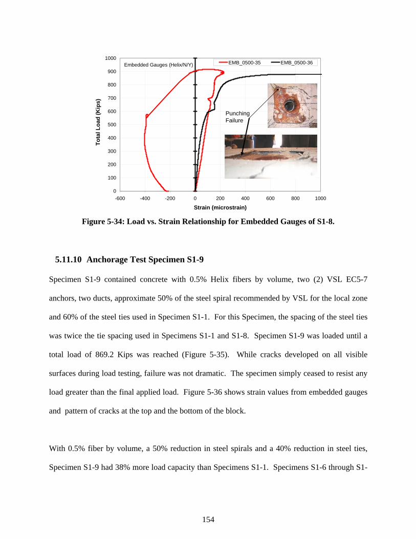
154
Embedded Gauges (Helix/N/Y)
0
100
200
300
400
500
600
700
800
900
1000
-600 -400 -200 0 200 400 600 800 1000
Strain (microstrain)
Tota
l Loa
d (K
ips)
EMB_0500-35 EMB_0500-36
PunchingFailure
Figure 5-34: Load vs. Strain Relationship for Embedded Gauges of S1-8.
5.11.10 Anchorage Test Specimen S1-9
Specimen S1-9 contained concrete with 0.5% Helix fibers by volume, two (2) VSL EC5-7
anchors, two ducts, approximate 50% of the steel spiral recommended by VSL for the local zone
and 60% of the steel ties used in Specimen S1-1. For this Specimen, the spacing of the steel ties
was twice the tie spacing used in Specimens S1-1 and S1-8. Specimen S1-9 was loaded until a
total load of 869.2 Kips was reached (Figure 5-35). While cracks developed on all visible
surfaces during load testing, failure was not dramatic. The specimen simply ceased to resist any
load greater than the final applied load. Figure 5-36 shows strain values from embedded gauges
and pattern of cracks at the top and the bottom of the block.
With 0.5% fiber by volume, a 50% reduction in steel spirals and a 40% reduction in steel ties,
Specimen S1-9 had 38% more load capacity than Specimens S1-1. Specimens S1-6 through S1-

155
9 were all cast from the same batch of concrete with 0.5% Helix fibers by volume. Specimen
S1-6 had no spiral or ties. Specimens S1-7 had spirals but not ties. Specimen S1-8 had ties but
no spirals. The load capacity of Specimen S1-9 was 45% and 28% greater than that of Specimen
S1-6 and Specimen S1-7, respectively. The load capacity for Specimen S1-9 was 5% less than
the load capacity of Specimen S1-8. Based upon these load tests, the presence of steel ties in the
general zone contributes more to load capacity than does the presence of spirals in the local zone.
Comparing Specimen S1-9 with Specimen S1-13 shows that the steel fibers contributed to a 19%
increase in load capacity.
0
100
200
300
400
500
600
700
800
900
1000
0 0.1 0.2 0.3 0.4 0.5 0.6 0.7 0.8
Deflection (in)
Tota
l Loa
d (K
)
S1-9 (Heli, 0.5, 0.6)PunchingShear & Bursting Cracks
Figure 5-35: Load vs. Deflection of S1-9.

156
0
200
400
600
800
1000
-500 -400 -300 -200 -100 0 100 200 300 400 500 600 700 800 900 1000
Strain (Microstrain)
Tota
l Loa
d (K
ips)
EMB_0500-34 EMB_0523-43
Bursting Cracks
294 microstrain
506 microstrain
Punching Shear
Figure 5-36: Load vs. Strain Relationship for Embedded Gauges of S1-9
5.11.11 Anchorage Test Specimen S1-10
Specimens S1-10, S1-11 and S1-14 were all cast from the same batch of concrete with 0.5%
Novomesh fibers by volume. In addition to the Novomesh fibers, Specimen S1-10 contained
two (2) VSL EC5-7 anchors and ducts. The specimen did not contain steel spirals and steel ties.
Specimen S1-10 was tested at the age of 149 days. The 28 day compressive strength and the 154
day compressive strength were 4305 psi and 5752 psi, respectively. The 28 day tensile strength
and the 154 day tensile strength were 410 psi and 295 psi, respectively. The failure load of 838.5
Kips was approximately 45% greater than twice the GUTS for each VSL anchor (2x289Kips =
578 Kips) and 34% greater than the maximum load applied to Specimen S1-1. The failure of
Specimen S1-10 was a sudden, explosive failure (Figure 5-37). The first visible surface crack
did not develop until a load of approximately 750 Kips was applied to the specimen (Figure
5-38). Steel ties were not present to resist the bursting tensile stresses.

157
0
100
200
300
400
500
600
700
800
900
1000
0 0.1 0.2 0.3 0.4 0.5 0.6 0.7 0.8
Deflection (in)
Tota
l Loa
d (K
ips)
S1-10 (Novomesh, N, N)
Figure 5-37: Load vs. Deflection of S1-10
0
200
400
600
800
1000
-500 -400 -300 -200 -100 0 100 200 300 400 500 600 700 800 900 1000
Strain (Microstrain)
Tota
l Loa
d (K
ips)
EMB_0523-52 EMB_0523-38
Figure 5-38: Load vs. Strain Relationship for Embedded Gauges of S1-10

158
5.11.12 Anchorage Test Specimen S1-11
Specimen S1-11 contained concrete with 0.5% Novomesh fibers by volume, two (2) VSL EC5-7
anchors, two ducts, and steel spirals. The specimen did not contain steel ties. Using the typical
load setup, Specimen S1-11 was loaded until it failed at a total load of 706.32 Kips (Figure
5-39). Specimen S1-11 was tested at the age of 149 days. The failure load for S1-11 was 22%
greater the GUTS for the two anchors and 12% greater than the load applied to Specimen S1-1.
However, the total load applied to Specimen S1-11 was 16% less than the load applied to
Specimen S1-10. Based upon the shape of Specimen S1-11, form racking occurred during the
casting of the specimen. The top and side surfaces of the specimen were slightly angled. This
may have contributed to the reduced load capacity. For both Dramix and Helix specimens, the
addition of spirals in the local zone resulted in an increase in load capacity not a decrease.
0
100
200
300
400
500
600
700
800
900
1000
0 0.1 0.2 0.3 0.4 0.5 0.6 0.7 0.8
Deflection (in)
Tota
l Loa
d (K
ips)
S1-11 (Novomesh, Y, N)SuddenPunching and SplittingFailure
Figure 5-39: Load vs. Deflection of S1-11
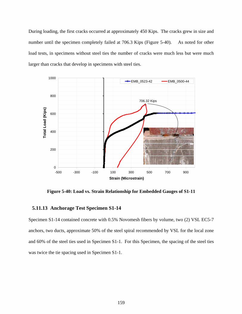
159
During loading, the first cracks occurred at approximately 450 Kips. The cracks grew in size and
number until the specimen completely failed at 706.3 Kips (Figure 5-40). As noted for other
load tests, in specimens without steel ties the number of cracks were much less but were much
larger than cracks that develop in specimens with steel ties.
0
200
400
600
800
1000
-500 -300 -100 100 300 500 700 900
Strain (Microstrain)
Tota
l Loa
d (K
ips)
EMB_0523-42 EMB_0500-44
706.32 Kips
Figure 5-40: Load vs. Strain Relationship for Embedded Gauges of S1-11
5.11.13 Anchorage Test Specimen S1-14
Specimen S1-14 contained concrete with 0.5% Novomesh fibers by volume, two (2) VSL EC5-7
anchors, two ducts, approximate 50% of the steel spiral recommended by VSL for the local zone
and 60% of the steel ties used in Specimen S1-1. For this Specimen, the spacing of the steel ties
was twice the tie spacing used in Specimen S1-1.

160
Specimen S1-14 was loaded until a total load of 995.59 Kips was reached. The Specimen did
not fail. The load application was stopped because the load limit for the load testing frame (1000
Kips) was reached, essentially. At the conclusion of the load test, there were no visible cracks
on the surface of Specimen S1-14. When the load was removed the specimen looked as if no
load had been applied. Figure 5-41 shows load vs. deflection relationship for S1-14.
0
100
200
300
400
500
600
700
800
900
1000
0 0.1 0.2 0.3 0.4 0.5 0.6 0.7 0.8 0.9 1
Deflection (in)
Tota
l Loa
d (K
)
S1-14 (Novomesh, 0.5,0.6)
Figure 5-41: Load vs. Deflection of S1-12
Considering a final load capacity in excess of 1000 Kips, Specimen S1-14 was greater than 59%
stronger than Specimen S1-1 and greater than 19% stronger than Specimen S1-10. Since
Specimen S1-14 had a load capacity that was over 1.36 times greater than that of Specimen S1-
13, the steel fibers contributed at least a 36% increase in load capacity.
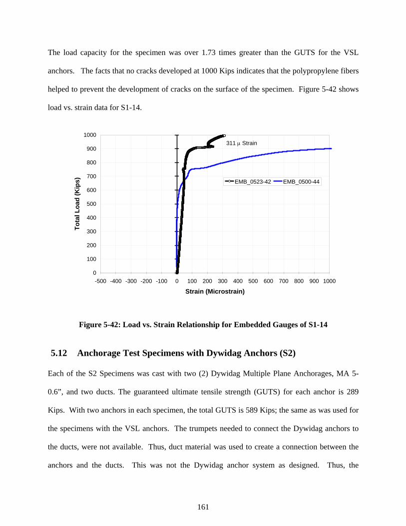
161
The load capacity for the specimen was over 1.73 times greater than the GUTS for the VSL
anchors. The facts that no cracks developed at 1000 Kips indicates that the polypropylene fibers
helped to prevent the development of cracks on the surface of the specimen. Figure 5-42 shows
load vs. strain data for S1-14.
0
100
200
300
400
500
600
700
800
900
1000
-500 -400 -300 -200 -100 0 100 200 300 400 500 600 700 800 900 1000
Strain (Microstrain)
Tota
l Loa
d (K
ips) EMB_0523-42 EMB_0500-44
311 μ Strain
Figure 5-42: Load vs. Strain Relationship for Embedded Gauges of S1-14
5.12 Anchorage Test Specimens with Dywidag Anchors (S2)
Each of the S2 Specimens was cast with two (2) Dywidag Multiple Plane Anchorages, MA 5-
0.6”, and two ducts. The guaranteed ultimate tensile strength (GUTS) for each anchor is 289
Kips. With two anchors in each specimen, the total GUTS is 589 Kips; the same as was used for
the specimens with the VSL anchors. The trumpets needed to connect the Dywidag anchors to
the ducts, were not available. Thus, duct material was used to create a connection between the
anchors and the ducts. This was not the Dywidag anchor system as designed. Thus, the

162
strengths obtained in the test program may have been affected by the absence of the trumpets.
However, since all of the S2 specimens were fabricated in the same way, strength comparisons
can still be made for the various fiber and steel combinations considered in the S2 specimens.
The bearing surface for all S2 specimens was a wooden sandbox.
5.12.1 Anchorage Test Specimen S2-1
Specimen S2-1 contained plain concrete, two Dywidag MA 5-0.6 anchors with ducts, two steel
spirals and steel ties. Specimens 2-1 was tested at the age of 55 days. The 28 day compressive
strength and the fifty-five (55) day compressive strength were 4406 psi and 5598 psi,
respectively. The 28 day tensile strength and the fifty-six (56) day tensile strength were 265 psi
and 275 psi, respectively.
The maximum load applied to the specimen was 723.25 Kips. This load was 1.25 times greater
than the GUTS for the two anchors. Figure 5-44 shows some punching did occur at the anchors.
However, this occurred near the upper limit of the load applied to the specimen. Failure
occurred due to the application of an excessive load; significant cracking and/or breaking of the
specimen occurred on all surfaces during the load test.

163
0
100
200
300
400
500
600
700
800
900
1000
0 0.1 0.2 0.3 0.4 0.5 0.6 0.7 0.8 0.9 1Deflection (in)
App
lied
Load
(Kip
s)
S2-1 (None/Y/Y)
Figure 5-43: Load vs. Deflection of S2-1
A major difference between Specimens S2-1 and Specimen S1-1 are the anchors that were
embedded in each; S2-1 had Dywidag anchors and S1-1 had VSL anchors. Another difference
was in the testing setup for the two specimens. At the bearing surface, for Specimen S1-1 a
neoprene bearing pad was used instead of the sandbox that was used for Specimen S2-1. The
maximum load applied to Specimen S2-1 was approximately 15% greater than the maximum
load applied to S1-1. However, the concrete compressive strength of the S2-1 was
approximately 15% less than the concrete strength of Specimen S1-1. The relationship between
load vs. strain measurements is shown in Figure 5-44.

164
0
100
200
300
400
500
600
700
800
900
1000
-500 -400 -300 -200 -100 0 100 200 300 400 500 600 700 800 900 1000
Strain (Microstrain)
Tota
l Loa
d (K
ips)
EMB_0523-56 EMB_0523-54
Figure 5-44: Load vs. Strain Relationship for Embedded Gauges of S2-1
5.12.2 Anchorage Test Specimen S2-14
Specimen S2-14 contained plain concrete two (2) Dywidag MA5-0.6” anchors, two ducts,
approximate 50% of the steel spiral recommended by Dywidag for the local zone and 60% of the
steel ties used in Specimen S2-1. For this specimen, the spacing of the steel ties was twice the
tie spacing used in Specimens S2-1 (and the same as that used in S1-2). At the bearing end of
the specimen, the specimen rested in a wooden sandbox.
Specimen S2-14 was tested at an age of 56 days. The first visible cracks on the surface of the
specimen did not develop until a load in excess of 600 kips was reached. Medium cracks exist
on all surfaces of the specimen. Bursting tension cracks are on the east and west faces of the
walls. Failure was initiated in the general zone of the anchorage specimen. The failure load

165
was 645.8 Kips (1.117 times greater than GUTS). Figure 5-45 load vs. deflection relationship,
and Figure 5-46 shows strain measurements of embedded gauges in S1-14.
0
100
200
300
400
500
600
700
800
900
1000
0 0.1 0.2 0.3 0.4 0.5 0.6 0.7 0.8 0.9 1
Defelction (in)
App
lied
Load
(Kip
s)
S2-14 (None/0.5/0.6)
Figure 5-45: Load vs. Deflection of S2-14
With approximately 50% of the spiral steel and 60% of the tie steel used in Specimen S2-1,
Specimen S2-14 had over 89% of the strength of Specimen S2-1. Except for the different
anchors and the different concrete strengths, Specimens S2-14 and S1-13 were similar. The total
load applied to S2-14 (646 Kips) was 12% less than the load applied to S1-13. As stated
previously, the concrete strength of Specimen S2-14 was over 15% less than that of Specimen
S1-13.

166
280.5 μ Strain
0
100
200
300
400
500
600
700
800
900
1000
-500 -400 -300 -200 -100 0 100 200 300 400 500 600 700 800 900 1000
Strain (Microstrain)
Tota
l Loa
d (K
ips)
EMB_1 EMB_2 EMB_3 EMB_4 EMB_5
Figure 5-46: Load vs. Strain Relationship for Embedded Gauges of S2-14
5.12.3 Anchorage Test Specimen S2-2
Specimen S2-2 contained concrete with 0.5% Dramix ZP305 fibers by volume, two (2) Dywidag
MA5-0.6” anchors and ducts. The specimen did not contain steel spirals and steel ties.
Specimens S2-2 through Specimen S2-5 were all cast from the same batch of concrete with 0.5%
Dramix ZP305 fibers by volume. Specimen S2-2 was tested at the age of 55 days. The 28 day
compressive strength and the 55 day compressive strength were 3463 psi and 4200 psi,
respectively. The 28 day split tensile strength and the 56 day split tensile strength were 323 psi
and 365 psi, respectively. The compressive strength of 4200 psi was slightly above the concrete
mix design strength of 4000 psi.
The failure load of 557.2 Kips (Figure 5-47) was approximately 4% less than twice the GUTS
for the anchors (578 Kips). The failure was sudden and without warning. The two factors which

167
most contributed to this reduced load capacity are absence of steel spirals and the absence of
steel ties. Even without the reinforcing steel, the load capacity of Specimen S2-2 was
approximately 77% of the load capacity of Specimen S2-1, which contained plain concrete, the
full Dywidag recommended spirals, and steel ties.
0
100
200
300
400
500
600
700
800
900
1000
0 0.1 0.2 0.3 0.4 0.5 0.6 0.7 0.8 0.9 1
Defelction (in)
App
lied
Load
(Kip
s)
S2-2 (Dramix/N/N)
Figure 5-47: Load vs. Deflection of S2-2
Figure 5-48 shows strain values from embedded gauges along with an image of the anchors
punching through the concrete. Large cracks developed on the east and west faces (short sides)
of the specimen. These cracks were very wide because steel tie reinforcement was not present to
distribute the tensile forces. Much smaller cracks developed on the north and south faces of the
specimen.

168
0
100
200
300
400
500
600
700
800
900
1000
-500 -300 -100 100 300 500 700 900
Defelction (in)
App
lied
Load
(Kip
s)EMB_0066-2EMB_0066-11
Figure 5-48: Load vs. Strain Relationship for Embedded Gauges of S2-2
5.12.4 Anchorage Test Specimen S2-3
Specimen S2-3 contained concrete with 0.5% Dramix ZP305 fibers by volume, two (2)
Dywidag MA5-0.6” anchors, two ducts, and steel spirals. The specimen did not contain steel
ties. Specimen S2-3 was tested at the age of 55 days. Using the typical load set-up, Specimen
S2-3 was loaded until it failed at a total load of 628.3 Kips (Figure 5-49).
The first visible crack developed at approximately 600 Kips. This crack developed on the north
face of the specimen. At the failure load, a large tension (bursting) crack developed on west face
(on a 19.5’’ side) of the specimen. Figure 5-50 shows strain measurements from embedded
gauges. As shown from the figure a very large crack developed on the west face of the specimen

169
at the failure load. At the final load magnitude, some punching did occur at the anchors. The
failure load of this specimen was approximately 13% higher than the failure load of Specimen
S2-2. Thus, test results indicate that the presence of spirals in the local zone contributes to a
13% increase in load capacity.
0
100
200
300
400
500
600
700
800
900
1000
0 0.1 0.2 0.3 0.4 0.5 0.6 0.7 0.8 0.9 1
Defelction (in)
App
lied
Load
(K)
S2-3 (Dramix/Y/N)
Figure 5-49: Load vs. Deflection of S2-3

170
0
100
200
300
400
500
600
700
800
900
1000
-500 -300 -100 100 300 500 700 900
Defelction (in)
App
lied
Load
(Kip
s)EMB_0085-7EMB_0085-3
Figure 5-50: Load vs. Strain Relationship for Embedded Gauges of S2-3
5.12.5 Anchorage Test Specimen S2-4
Specimen S2-4 contained concrete with 0.5% Dramix ZP305 fibers by volume, two (2) Dywidag
MA5-0.6” anchors, two ducts, and steel ties. The specimen did not contain steel spirals.
Specimen S2-4 was loaded until the total load of 673.97 kips was applied (Figure 5-51). During
testing, the first visible crack developed on the north face at a load of approximately 560 kips.
At the failure load, the specimen could not maintain the applied load. Therefore, the load test
was stopped. Figure 5-52 shows the load vs. strain relationship of embedded gauges in the
specimen.

171
The failure load was approximately 17% greater than GUTS for the anchors, 7% less than the
load applied to Specimen S2-1, 21% greater than the load applied to S2-2 and 7% greater than
the load applied to S2-3. Thus, the presence of ties without spirals results in more than a 21%
increase in load capacity above the capacity of the specimen with 0.5% Dramix fibers by volume
without ties and spirals, Specimen S2-2.
0
100
200
300
400
500
600
700
800
900
1000
0 0.1 0.2 0.3 0.4 0.5 0.6 0.7 0.8 0.9 1
Defelction (in)
App
lied
Load
(Kip
s)
S2-4 (Dramix/N/Y)
Figure 5-51: Load vs. Deflection of S2-4

172
0
100
200
300
400
500
600
700
800
900
1000
-400 -200 0 200 400 600 800 1000
Defelction (in)
App
lied
Load
(Kip
s)
EMB_0060-11EMB_0060-2
Figure 5-52: Load vs. Strain Relationship for Embedded Gauges of S2-4
5.12.6 Anchorage Test Specimen S2-5
Specimen S2-5 contained concrete with 0.5% Dramix ZP305 fibers by volume, two (2) Dywidag
MA5-0.6” anchors, two ducts, approximate 50% of the steel spiral recommended by Dywidag
for the local zone and 60% of the steel ties used in Specimen S2-1. For this Specimen, the
spacing of the steel ties was twice the tie spacing used in Specimens S2-1 and S2-3. Specimen
S2-5 was loaded until a total load of 665.56 Kips was reached.
The first cracks developed a total load in excess of 500 Kips. At the failure load, approximately
666 Kips, the specimen ceased to maintain the applied load (Figure 5-53). Thus, the load test
was stopped. Some punching of the anchors did occur. Based upon the crack pattern, it appears
that the failure of the specimen was due to both local and general zone failure. Figure 5-54
shows load vs. strain relationship for the two embedded gauges in the block.

173
0
100
200
300
400
500
600
700
800
900
1000
0 0.1 0.2 0.3 0.4 0.5 0.6 0.7 0.8 0.9 1
Defelction (in)
App
lied
Load
(Kip
s)S2-5 (Dramix/0.5/0.6)
Figure 5-53: Load vs. Deflection of S2-5
With 0.5% fiber by volume, a 50% reduction in steel spirals and a 40% reduction in steel ties,
Specimen S2-5 had 8% less load capacity than Specimen S2-1. Specimens S2-2 through S2-5
were cast from the same batch of concrete with 0.5% Dramix fibers by volume. Specimen S2-2
had no spiral or ties. Specimens S2-3 had spirals but not ties. Specimen S1-4 had ties but no
spirals. The load capacity of Specimen S2-5 was 8% less, 19% greater, 6% greater and 1% less
than the strengths of Specimens S2-1, S2-2, S2-3, and S2-4, respectively. Although the strength
of S2-5 was less than that of Specimen S2-1, load capacity of S2-5 was 15% greater than the
GUTS for the anchors. Figure 5-54 shows load vs. strain data for Specimen S2-5.

174
0
100
200
300
400
500
600
700
800
900
1000
-400 -200 0 200 400 600 800 1000
Strain (Microstrain)
Tota
l Loa
d (K
ips)
EMB_0066-6 EMB_0060-9
Figure 5-54: Load vs. Strain Relationship for Embedded Gauges of S2-5
5.12.7 Anchorage Test Specimen S2-6
Specimens S2-6, S2-7, S2-8 and S2-9 were all cast from the same batch of concrete, which
contained 0.5% Helix fiber by volume. Specimen S2-6 contained concrete with 0.5% Helix
fibers by volume, two (2) Dywidag MA5-0.6” anchors and ducts. The specimen did not contain
steel spirals and did not contain steel ties. Specimen S2-6 was tested at the age of 56 days. The
28 day compressive strength and the 56 day compressive strength were 4550 psi and 5757 psi,
respectively. The 28 day split tensile strength and the 56 day split tensile strength were 361 psi
and 388 psi, respectively. The failure load of 567.7 Kips was approximately 2% less than the
GUTS for the two anchors (578 Kips).

175
0
100
200
300
400
500
600
700
800
900
1000
0 0.1 0.2 0.3 0.4 0.5 0.6 0.7 0.8 0.9 1
Defelction (in)
App
lied
Load
(Kip
s) S2-6 (Helix/N/N)
Figure 5-55: Load vs. Deflection of S2-6
The first visible surface crack occurred at approximately 450 Kips. During the load test, cracks
developed on all visible surfaces of the Specimen (Figure 5-55 and Figure 5-56). For this
specimen, failure resulted from punching shear at the anchors. The absence of steel spirals
contributed to this result. The compressive strength and the tensile strength of the concrete in
Specimen S2-6 was greater than the strengths of the concrete in the S2-1 Specimen. However,
the failure load of Specimen S2-6 was 22% less than the failure load for S2-1. Comparing S2-6
with S2-2, reveals that the two Specimens broke at approximately the same strength (an average
of about 97% of the GUTS load for the two anchors); the failure load for Specimen S2-6 was
approximately 2% greater than the failure load of Specimen S2-2. Both of these specimens had
steel fibers but did not have any other steel reinforcement.

176
0
100
200
300
400
500
600
700
800
900
1000
-400 -200 0 200 400 600 800 1000
Strain (Microstrain)
Tota
l Loa
d (K
ips)
EMB_0500-32 EMB_0500-45
Vertical cracks
Figure 5-56: Load vs. Strain Relationship for Embedded Gauges of S2-6
5.12.8 Anchorage Test Specimen S2-7
Specimen S2-7 contained concrete with 0.5% Helix fibers by volume, two (2) Dywidag MA5-
0.6” anchors, two ducts, and two steel spirals. The specimen did not contain steel ties. Specimen
S2-7 was tested at the age of 56 days. Using the typical load set-up (the same as used for all
specimens except S2-1), Specimen S2-7 was loaded until it failed at a total load of 691.14 Kips
(Figure 5-57).
The first visible cracks developed on the north and west sides of the specimen at an approximate
applied load of 400 Kips. Failure was noted when the specimen ceased to withstand additional
applied load; an increase in load resulted in an increase in deflection which prevented resistance
of the load. The failure load for Specimen S2-7 was approximately 20% greater than the GUTS

177
for the two anchors. The strength capacity of Specimen S2-7 was 4% less than that of Specimen
S2-1.
0
100
200
300
400
500
600
700
800
900
1000
0 0.1 0.2 0.3 0.4 0.5 0.6 0.7 0.8 0.9 1
Defelction (in)
App
lied
Load
(Kip
s)
S2-7 (Helix/Y/N)
Figure 5-57: Load vs. Deflection of S2-7
Comparing the ultimate load applied to Specimens S2-7 and S2-6, revealed that the inclusion of
spirals in the local zone contributed to a 22% increase in load capacity. A relatively small
displacement of the anchors (punching) did occur in Specimen S2-7. Cracks developed on all
surfaces of the specimen. The crack widths were small to medium. The cracks appear larger in
the photographs because (to increase visibility) the cracks were traced with a marker. Figure
5-58 presents the load-strain relationship for the two embedded gauges inside the specimen.

178
0
100
200
300
400
500
600
700
800
900
1000
-400 -200 0 200 400 600 800 1000
Strain (Microstrain)
Tota
l Loa
d (K
ips)
EMB_0060-1
EMB_0060-3
Figure 5-58: Load vs. Strain Relationship for Embedded Gauges of S2-7
5.12.9 Anchorage Test Specimen S2-8
Specimen S2-8 contained concrete with 0.5% Helix fibers by volume, two (2) Dywidag MA5-
0.6” anchors, two ducts, and steel ties. The specimen did not contain steel spirals. Specimen
S2-8 was loaded until the total load of 747.7 kips was applied (Figure 5-59). Figure 5-60
presents load vs. strain measurements. Also, it can be seen that some displacement of the
anchors did occur during testing. The first cracks on the specimen developed at an applied load
of approximately 675 Kips. Cracks developed on all surfaces of the specimen. Some cracks
initiated on the bearing surface and some cracks initiated on the load surface at or near the
anchors. Both local and general zone failure occurred in this specimen.
At the maximum applied load, the specimen would not adequately resist additional loads; the
system load would not stabilize. A 747.7 K final load was 1.03 times greater than the load

179
applied to Specimen S2-1 and 1.29 times greater than the GUTS load for the Dywidag anchors.
Comparing the ultimate load applied to S2-8 and the ultimate load applied to S2-6 (which has
0.5% fiber but no spirals and no ties) showed that the presence of steel ties results in a 32%
increase in load capacity. This increase in strength attributable to ties in the specimen with
Helix fibers was greater than the 21% increase attributable to ties in the specimen with Dramix
fibers.
0
100
200
300
400
500
600
700
800
900
1000
0 0.1 0.2 0.3 0.4 0.5 0.6 0.7 0.8 0.9 1Defelction (in)
App
lied
Load
(Kip
s)
S2-8 (Helix/N/Y)Bursting crack
Figure 5-59: Load vs. Deflection of S2-8

180
0
100
200
300
400
500
600
700
800
900
1000
-400 -200 0 200 400 600 800 1000
Strain (Microstrain)
Tota
l Loa
d (K
ips)
EMB_0500-48 EMB_0500-42
Figure 5-60: Load vs. Strain Relationship for Embedded Gauges of S2-8
5.12.10 Anchorage Test Specimen S2-9
Specimen S2-9 contained concrete with 0.5% Helix fibers by volume, two (2) Dywidag MA5-
0.6” anchors, two ducts, approximate 50% of the steel spirals recommended by Dywidag for the
local zone and 60% of the steel ties used in Specimen S2-1. For this specimen, the spacing of
the steel ties was twice the tie spacing used in Specimens S2-1, S2-4 and S2-8. Specimen S2-9
was loaded until a total load of 752.594 Kips was reached (Figure 5-61). This load was 30%
greater than the GUTS for the two anchors.
The first crack (a crack on the north face) occurred at the bottom of the specimen at
approximately 550 Kips. The second crack (also on the north face starting at the bottom)
occurred at approximately 740 Kips. At the maximum applied load, the specimen would not
adequately resist additional loads; the magnitude of the applied load would not stabilize due to

181
deflection of the specimen at the load application points. At the end of the load cycle, only small
width cracks existed on the surfaces of the specimen. However, it appears that the failure was
due to both local and general zone failure; failure of the local anchorage zone was apparent.
Figure 5-61 shows the surfaces of Specimen S2-9 after the load after the load test was complete.
0
100
200
300
400
500
600
700
800
900
1000
0 0.1 0.2 0.3 0.4 0.5 0.6 0.7 0.8 0.9 1Defelction (in)
App
lied
Load
(Kip
s)
S2-9 (Helix/0.5/0.6)
Figure 5-61: Load vs. Deflection of S2-9
With 0.5% fiber by volume, a 50% reduction in steel spirals and a 40% reduction in steel ties,
Specimen S2-9 had 4% more load capacity than Specimen S2-1. Specimens S2-6 through S2-9
were all cast from the same batch of concrete with 0.5% Helix fibers by volume. Specimen S2-6
had no spiral or ties. Specimen S2-7 had spirals but no ties. Specimen S2-8 had ties but no
spirals. Specimen S2-9 had 33%, 9% and 1% greater load capacity of than did specimen S2-6,
Specimen S2-7 and Specimen S2-8, respectively. Figure 5-62 shows load-strain data for
Specimen S2-9.

182
0
100
200
300
400
500
600
700
800
900
1000
-400 -300 -200 -100 0 100 200 300 400 500 600 700 800 900 1000Strain (Microstrain)
Tota
l Loa
d (K
)EMB_0062-10 EMB_0060-8
Figure 5-62: Load vs. Strain Relationship for Embedded Gauges of S2-9
5.12.11 Anchorage Test Specimen S2-10
Specimens S2-10, S2-11, S2-12 and S1-13 were all cast from the same batch of concrete with
0.5% Novomesh fibers by volume. In addition to the Novomesh fibers, Specimen S2-10
contained two (2) Dywidag MA5-0.6” anchors and two ducts. The specimen did not contain
steel spirals and steel ties. Specimen S2-10 was tested at the age of 57 days. The 28 day
compressive strength and the 61 day compressive strength were 4127 psi and 5179 psi,
respectively. The 28 day tensile strength and the 61 day tensile strength were 410 psi and 295
psi, respectively.
The first crack developed on the east side of the specimen at an applied load of approximately
600 Kips. The failure of Specimen S2-10 was sudden and due to punching shear. As a result of
the punching shear failure, major tension cracks developed on the east and west faces (short
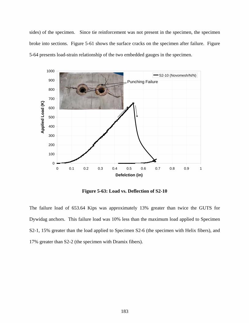
183
sides) of the specimen. Since tie reinforcement was not present in the specimen, the specimen
broke into sections. Figure 5-61 shows the surface cracks on the specimen after failure. Figure
5-64 presents load-strain relationship of the two embedded gauges in the specimen.
0
100
200
300
400
500
600
700
800
900
1000
0 0.1 0.2 0.3 0.4 0.5 0.6 0.7 0.8 0.9 1
Defelction (in)
App
lied
Load
(K)
S2-10 (Novomesh/N/N)
Punching Failure
Figure 5-63: Load vs. Deflection of S2-10
The failure load of 653.64 Kips was approximately 13% greater than twice the GUTS for
Dywidag anchors. This failure load was 10% less than the maximum load applied to Specimen
S2-1, 15% greater than the load applied to Specimen S2-6 (the specimen with Helix fibers), and
17% greater than S2-2 (the specimen with Dramix fibers).

184
0
100
200
300
400
500
600
700
800
900
1000
-400 -300 -200 -100 0 100 200 300 400 500 600 700 800 900 1000Strain (Microstrain)
Tota
l Loa
d (K
ips)
EMB_0066-3 EMB_0066-10
Figure 5-64: Load vs. Strain Relationship for Embedded Gauges of S2-10
5.12.12 Anchorage Test Specimen S2-11
Specimen S2-11 contained concrete with 0.5% Novomesh fibers by volume, two (2) Dywidag
MA5-0.6” anchors, two ducts, and steel spirals. The specimen did not contain steel ties.
Specimen S2-11 was tested at the age of 57 days. Using the typical load setup, Specimen S2-11
was loaded until it failed at a total load of 569.723 Kips (Figure 5-65).
The first cracks occurred on the north and south faces of the specimen at approximately 450
Kips. The failure at approximately 570 Kips was accompanied by a small “thud”. Figure 5-65
shows the failed Specimen S2-11, and Figure 5-66 presents load-strain relationship. The failure
load for S2-11 was approximately 99% of the GUTS for the two anchors and 21% less than the
load applied to Specimen S2-1. The maximum load applied to Specimen S2-11 was only 91%
and 82% of the total load applied to Specimens S2-3 and S2-7, respectively.

185
0
100
200
300
400
500
600
700
800
900
1000
0 0.1 0.2 0.3 0.4 0.5 0.6 0.7 0.8 0.9 1Defelction (in)
App
lied
Load
(K)
S2-11 (Novomesh/Y/N)
BurstingCrack
PunchingFailure
Figure 5-65: Load vs. Deflection of S2-11
0
100
200
300
400
500
600
700
800
900
1000
-400 -300 -200 -100 0 100 200 300 400 500 600 700 800 900 1000Strain (Microstrain)
Tota
l Loa
d (K
ips)
EMB_0523-41
EMB_0500-46
570 Kips
Punching Failure
Figure 5-66: Load vs. Strain Relationship for Embedded Gauges of S2-11

186
5.12.13 Anchorage Test Specimen S2-12
Specimen S2-12 contained concrete with 0.5% Novomesh fibers by volume, two (2) Dywidag
MA5-0.6” anchors, two ducts, and steel ties. The specimen did not contain steel spirals.
Specimen S2-12 was loaded at an age of 61 days until a total load of 750 Kips was reached
(Figure 5-67). The first crack on the surface of the specimen was not visible until approximately
750 Kips, just prior to the final load application. At higher loads, visible displacement of the
anchors occurred such that additional load was not resisted by the specimen. Figure 5-68
presents load-strain relationship. The final load of 750 Kips was 4% greater than the load
capacity of Specimen S2-1 and approximately 30% greater than the GUTS for the anchors in the
specimen. The strength of S2-12 was 15% greater than S2-10 and 32% greater than Specimen
S2-11.
0
100
200
300
400
500
600
700
800
900
1000
0 0.1 0.2 0.3 0.4 0.5 0.6 0.7 0.8 0.9 1Defelction (in)
App
lied
Load
(Kip
s)
S2-12 (Novomesh/N/Y)
Figure 5-67: Load vs. Deflection of S2-12

187
0
100
200
300
400
500
600
700
800
900
1000
-400 -300 -200 -100 0 100 200 300 400 500 600 700 800 900 1000Strain (Microstrain)
Tota
l Loa
d (K
ips)
EMB_0065-6 EMB_0065-9
Figure 5-68: Load vs. Strain Relationship for Embedded Gauges of S2-12
5.12.14 Anchorage Test Specimen S2-13
Specimen S2-13 contained concrete with 0.5% Novomesh fibers by volume, two (2) Dywidag
MA5-0.6” anchors, two ducts, approximate 50% of the steel spiral recommended by Dywidag
for the local zone and 60% of the steel ties used in Specimen S2-1. For this Specimen, the
spacing of the steel ties was twice the tie spacing used in Specimens S2-1, S2-4, S2-8 and S2-12.
At an age of 61 days, Specimen S2-13 was loaded until a total load of 752.68 Kips was reached
(Figure 5-69). At this load, only hairline cracks were on the surface of the specimen. The failure
was a local zone failure of the anchor system. Load-strain relationships of embedded gauges are
presented in Figure 5-70.

188
The final load applied to Specimen S2-13 was 4% greater than the load applied to S2-1. The
load was 30% greater than the GUTS for the Specimen. The load capacity for Specimen S2-13
was approximately the same as the capacity for S2-12. This further indicates that the failure was
due to local zone failure in the vicinity of the anchorage system. Essentially, Specimens S2-8,
S2-9, S2-12 and S2-13 all failed at approximately 752 Kips and the failure appeared to be due to
failure in the local anchorage zone.
0
100
200
300
400
500
600
700
800
900
1000
0 0.1 0.2 0.3 0.4 0.5 0.6 0.7 0.8 0.9 1
Defelction (in)
App
lied
Load
(K)
S2-13 (Novomesh/0.5/0.6)
Local Zone Failure
Figure 5-69: Load vs. Deflection of S2-13

189
0
100
200
300
400
500
600
700
800
900
1000
-400 -300 -200 -100 0 100 200 300 400 500 600 700 800 900 1000Strain (Microstrain)
Tota
l Loa
d (K
)EMB_1 EMB_2 EMB_3
EMB_4 EMB_5 EMB_6
752.68 Kips
Figure 5-70: Load vs. Strain Relationship for Embedded Gauges of S2-13
5.13 Discussion of Anchorage Specimens Test Results
In this section the load test results for the various test specimens are summarized. An attempt is
made to discuss in brief the relevant findings from the two sets of test specimens. The discussion
includes a comparison of the performance of the S1 and S2 specimens. Table 5-1, Figure 5-71
Figure 5-72 show comparison of the two sets of specimens based on the maximum applied load
(kips) and development of first crack.

190
Table 5-1: Comparison of the Two Sets S1 and S2
Specimen Fiber/Spiral/Ties Failure Load (Kips)
First Crack (Kips)
Observations
S1-1 None/Y/Y 627.9 400+ S1-2 Dramix/N/N 794.0 287 Major Bursting Tension Crack on E and W Faces S1-3 Dramix/Y/N 865.6 830+ S1-4 Dramix/N/Y 999.2 1000 Stopped at 1000K, No visible cracks on the surfaces S1-5 Dramix/0.5/0.6 1000.4 1000 Stopped At 1000K, Few small cracks E sides. Cracks on bottom. S1-6 Helix/N/N 600.0 535+ Punching Shear. Loud boom At failure. S1-7 Helix/Y/N 677.2 S1-8 Helix/N/Y 916.7 800 S1-9 Helix/0.5/0.6 869.2 Specimen Began to Loose Load; Ceased to accept additional load. S1-10 Novomesh/N/N 838.5 750 Sudden, explosive failure. S1-11 Novomesh/Y/N 706.3 450 S1-13 None/0.5/0.6 732.5 500 S1-14 Novomesh/0.5/0.6 995.6 NA Load Stopped At 995K, No visible cracks at 980K.
S2-1 None/Y/Y 723.2 Punching Shear (Test Not Observed by FAM/FSU) S2-2 Dramix/N/N 557.2 550 Sudden Failure S2-3 Dramix/Y/N 628.3 600 Large Crack on West face. S2-4 Dramix/N/Y 674.0 560 Specimen Began to Loose Load; Ceased to accept additional load. S2-5 Dramix/0.5/0.6 665.6 500+ Specimen Began to Loose Load; Ceased to accept additional load. S2-6 Helix/N/N 567.7 450 Bursting Tension, Punching Shear S2-7 Helix/Y/N 691.1 400 Specimen Began to Loose Load; Ceased to accept additional load. S2-8 Helix/N/Y 747.7 675 Only minor cracks at 725K S2-9 Helix/0.5/0.6 752.6 550 Specimen Began to Loose Load; Failure of Anchor System. S2-10 Novomesh/N/N 653.6 600 Punching/Bursting Tension S2-11 Novomesh/Y/N 569.7 450 Sudden/ Small Thud/ Bursting Tension S2-12 Novomesh/N/Y 750.1 720+ Sudden, Soft Punching (displacement) of anchors. S2-13 Novomesh/0.5/0.6 752.7 550 Specimen Began to Loose Load; Ceased to accept additional load. S2-14 None/0.5/0.6 645.8 600+ Bursting Tension Crack on E and W Faces

191
794 86
6
999
1000
600 67
7
917
869
839
706 733
996
628
0
200
400
600
800
1000
1200
None/Y
/Y
Dramix/
N/N
Dramix/
Y/N
Dramix/
N/Y
Dramix/
0.5/0.
6
Helix/N
/N
Helix/Y
/N
Helix/N
/Y
Helix/0
.5/0.6
Novom
esh/N
/N
Novom
esh/Y
/N
None/0
.5/0.6
Novom
esh/0
.5/0.6
Specimen
Failu
re L
oad
(kip
s)
S1 Specimens
Figure 5-71: Load Capacity for S1 Specimens
557 62
8 674
666
568
691 74
8
753
654
570
750
753
64672
3
0
200
400
600
800
1000
1200
None/Y
/Y
Dramix/
N/N
Dramix/
Y/N
Dramix/
N/Y
Dramix/
0.5/0.
6
Helix/N
/N
Helix/Y
/N
Helix/N
/Y
Helix/0
.5/0.6
Novom
esh/N
/N
Novom
esh/Y
/N
Novom
esh/N
/Y
Novom
esh/0
.5/0.6
None/0
.5/0.6
Specimen
Failu
re L
oad
(kip
s)
S2 Specimens
Figure 5-72: Load Capacity for S2 Specimens
192
5.13.1 Discussion of VSL Anchor Test Specimens Results
A review of the results for the S1 test specimens, specimens cast with VSL anchors, showed that
adding steel fibers to the concrete mix did improve the performance of concrete in post-tensioned
anchorage zones. This was true for all three of the fiber types.
Comparing specimens cast with Dramix ZP305 fibers with plain concrete specimens showed that
steel fibers provide enough tensile strength such that it was possible to totally eliminate both
steel spirals and ties without reducing the load capacity of the specimen. In fact, for Specimen
S1-2, the load capacity was 26% greater than that of Specimen S1-1. The Dramix Specimen S1-
3 indicated that adding steel spiral with the steel fibers in the local anchorage zone resulted in a
9% increase in strength. While the Dramix Specimen S1-4 showed that adding steel ties with the
steel fibers resulted in a 26% increase in strength. However, the test results showed that spiral
reinforcement was necessary to prevent sudden failure due to punching shear and tie
reinforcement was necessary to prevent sudden failure due to excessive bursting tension. Thus,
it was not feasible to totally eliminate non-prestressed reinforcement. Yet, consideration of
Dramix Specimen S1-5 clearly showed that it was possible to greatly reduce the amount of non-
prestressed reinforcement when steel fiber reinforcement was added to the concrete. The load
capacity of Specimen S1-5 was over 1.59 times greater than the capacity of Specimen S1-1 with
plain concrete and full spiral and tie reinforcement. Comparing Specimen S1-5 and Specimen
S1-13 clearly showed that adding steel fibers greatly improved the load capacity of the
anchorage zone. While both specimens had 50% less spirals and 40 % less ties than S1-1, the
difference in the two specimens is that S1-5 had 0.5% steel fiber by volume and S1-13 had plain
concrete (no steel fibers). The use of the steel fibers resulted in a 37% increase in load capacity.
193
In addition to improving load capacity, the presence of steel fibers resulted in less surface crack
development. This can be a significant factor relating to durability of structural elements.
The beneficial effects of adding steel fibers to the anchorage zone was also evident by comparing
the different specimens cast with Helix fibers. Although, the specimen that was cast with 0.5%
Helix fiber and without any non-prestressed reinforcement (Specimen S1-6) did not have as great
a load capacity as Specimen S1-1; the load capacity of Specimen S1-6 was 96% as great as the
load capacity of Specimen S1-1. This was so even though the concrete compressive and tensile
strengths for Specimen S1-6 were significantly less than the concrete strengths of Specimen S1-
1. This showed that the addition of steel fibers did contribute to increased strength in the
anchorage zone. The Helix Specimen S1-7 indicated that adding steel spiral in the local
anchorage zone resulted in a 13% increase in strength. The Helix Specimen S1-8 showed that
adding steel ties resulted in a 53% increase in strength. Thus, the Helix fibers coupled with steel
ties resulted in a very large increase in load capacity. As was stated for the Dramix Specimen,
the load test results showed that adding Helix steel fibers resulted in increased strength and an
improved failure mechanism when steel spirals and ties were present. Helix Specimen S1-9,
which had 0.5% fiber, 50% steel spiral and 40% steel ties, was loaded to a 19% higher load
capacity than Specimen S1-13, which had plain concrete, 50% steel spiral and 40% steel ties.
The load capacity of Specimen S1-9 was over 1.38 times greater than the capacity of Specimen
S1-1 with plain concrete and full spiral and tie reinforcement. Thus, steel fibers did increase the
strength and improve the behavior of local and general post-tensioned anchorage zones.
194
Using Novomesh steel and polypropylene fibers resulted in improved strengths in the anchorage
zone also. Specimen S1-10 was cast with steel fibers but without other steel reinforcement in the
local and general anchorage zones. The load test results showed that the load capacity of S1-10
was 34% greater than that of S1-1 which had plain concrete and 100% steel spirals and 100%
steel ties. While Specimen S1-11, which had 0.5% fiber and spirals, had less load capacity that
S1-10, the capacity of S1-11 was 12% greater than that of S1-1. The reduced load capacity of
S1-11 may have been due to a small degree of raking of the forms during pouring. In spite of
this, the Novomesh fibers contributed to an increase of load capacity. The load capacity of
Specimen S1-14 was greater than 1000 K, the capacity of the load frame. The load application
was stopped prematurely due to the close proximity of the applied load to the load frame
capacity. Novomesh Specimen S1-14, which had 0.5% fiber, 50% steel spiral and 40% steel
ties, was loaded to a 36% higher load capacity than Specimen S1-13, which had plain concrete,
50% steel spiral and 40% steel ties. This Novomesh Specimen S1-14 performed similarly to the
Dramix Specimen S1-5. Possibly, the Helix Specimen S1-9 would have achieved a higher
strength, similar to the strengths of S1-5 and S1-14, if the concrete strength for the Helix
specimen was not reduced. In summary, the load test results for the S1 Specimens showed that
adding 0.5% steel fibers by volume to the concrete mix improved the load capacity of the
anchorage zones to the degree that the spiral and tie reinforcement could be greatly reduced by
50% and 40%, respectively. The spiral and tie reinforcement should not be totally eliminated.
5.13.2 Discussion of Dywidag Anchor Test Specimens Results
For the greatest failure loads applied to the S2 Specimens which contained Dywidag anchors, the
loads caused failure in the local and the general zones. In several specimens, deflection at the

195
anchors prevented the specimen from resisting additional loads. Thus, the failure loads were
closer to the limiting loads, Guaranteed Ultimate Strength, of the anchor systems. Yet, the S2
Specimen test results do indicate that steel fibers improve the tensile strength of the anchorage
zones. As was the case for the S1 Specimens, with 0.5% steel fibers in the concrete mix, the
addition of steel spirals resulted in an increase in load capacity. The addition of steel ties
resulted in a greater strength increase than was found for the spirals.
For S2 Specimens with 0.5% Dramix fibers, Specimen S2-2, which had no spirals or ties, had
77% of the load capacity of the S2-1 Specimen which had plain concrete and 100% of steel
spirals and 100% of steel ties based upon design recommendations. Similarly, the specimens
with 0.5% Helix fiber (Specimen S2-6) and 0.5% Novomesh fibers (Specimen S2-10) had 78%
and 90% the load capacity of Specimen S2-1. Thus, fibers in concrete contributes to a the
specimens having a load capacity of 77% to 90% of the strength of the sections with steel spirals
and ties with plain concrete. The Dramix Specimens S2-3 and S2-4 showed that adding steel
spirals and steel ties added 13% and 21%, respectively, to the strength of the sections. Although
Specimen S2-5 had less capacity than S2-1, the measured load capacity for S2-5 showed that the
strength achieved by using 0.5% steel fibers by volume, 50% steel spirals and 40% steel ties was
92% of the load capacity of Specimen S2-1 and 15% greater than the GUTS strength of the two
PT anchors. Thus, it was feasible to achieve more than adequate strength in the anchorage zone
using 0.5% steel fiber and significant reductions in non-prestressed reinforcement.
Considering the Helix Specimens S2-7 and S2-8 showed that adding steel spirals and steel ties
with the 0.5% fiber resulted in a 22% and a 32%, increase in load capacity. The presence of steel

196
ties contributed greater strength than the presence of steel spirals. The measured load capacity
for S2-9 showed that the strength achieved by using 0.5% steel fibers, 50% steel spirals and 40%
steel ties was 104% of that of Specimen S2-1. Thus, adding Helix steel fibers and reducing the
non-prestressed reinforcement yielded a specimen 4% stronger than the plain concrete specimen
with full spirals and ties. The presence of steel fibers did improve the load carrying ability of
the anchorage zone.
Novomesh S2-11 did not show an increase in load capacity due to the addition of spirals; it
showed a 13% decrease in load capacity. However, the maximum applied load was 99% of the
GUTS load for the specimen. Since the maximum anticipated post-tensioning force is 80% of
the GUTS load, the strength of the specimen was more than adequate. In addition, it is not
recommended that an anchorage zone be constructed without steel ties. The load capacity of S2-
12 showed a 15% increase in capacity over S2-10 due to the addition of steel ties. Specimen S2-
13 with 0.5% fibers, 50% steel spirals and 40% steel ties had 4% greater load capacity than did
Specimen S2-1. Since Specimens S2-8, S2-9, S2-12 and S2-13 all failed at approximately the
same load, approximately 750 K, this seems to be the upper limit of the specimens ability to
resist the general zone bursting tensile forces and the compression forces in the local zone. The
upper limit on strength capacity for these four specimens was 4% greater than the strength
capacity of specimen S2-1 and 30% greater than the GUTS for the two anchors. Comparing
Specimens S2-5, S2-9 and S2-13, to Specimen S2-14 which was cast with the same reinforcing
configuration but plain concrete instead of fibers, showed that the addition of steel fibers resulted
in strength increase of 3% to 17%. From these tests, it is evident that adding fibers to the
anchorage zones resulted in increased load capacities which were more than adequate for the

197
strength of the PT anchors even when the non-prestressed reinforcement was significantly
reduced.
5.13.3 PT Anchor Test Specimens Results Summary
In summary, consideration of both S1 Specimens test results and S2 Specimens test results
showed the following:
1. Adding 0.5% steel fibers to the concrete mix without adding non-prestressed
reinforcement in the local and general anchorage zones resulted in test specimens having load
capacities that ranged from 77% to 134% of the load capacity of test specimens with plain
concrete and 100% of the local zone reinforcement recommended by the anchorage manufacturer
and 100% of the general zone reinforcement recommended by the approximate design method of
the AASHTO code.
2. Adding steel spirals along with the 0.5% steel fibers resulted in strength increases of up
to 22%. However, for two specimens cast with Novomesh fibers (S1-11 and S2-11) the addition
of spiral did not result in increases in strength instead a 13% to 17% decrease in strength
resulted.
3. Adding steel ties along with the 0.5% steel fibers resulted in strength increases of up to
32%.
4. Even though the addition of 0.5% steel fibers did add up to 37% increase in strength to
test specimens, steel spirals and steel ties are needed to prevent sudden failure due to punching
shear at the anchors (in the local zone) and to prevent sudden failure due to bursting tension in
the general zones.

198
5. With 0.5% fibers by volume, 50% of steel spirals (recommended by PT anchor
manufacturers) and 40% of steel ties (based upon AASHTO design guidelines) , the load
capacities of the anchorage zone test specimens were from 92% to 159% the load capacity of the
plain specimens with the recommend local and general zone reinforcement. Thus, the addition
of steel fibers did increase the strength of the anchorage zone even with reductions in non-
prestressed reinforcing steel.
6. In addition, to improving the strength of the specimens, the addition of fibers (steel and steel
and polypropylene fibers) resulted in smaller and few cracks developing on the surface of the test
specimens. Thus, the use of fibers in PT anchorage zones may contribute to improvements in the
durability of structural elements.

199
CHAPTER 6
COMPARISON OF NUMERICAL ANALYSIS AND EXPERIMENTAL RESULTS
6.1 Numerical Modeling of Laboratory Specimens
As stated in Chapter 4, the geometry of the block specimens used in laboratory testing was based
on prior finite element analysis on a typical bridge segment to determine the magnitudes and
distribution of the stresses in the anchor zone and on the AASHTO requirements for the general
zone size. After the completion of laboratory tests on anchor specimens, another round of finite
element analysis was conducted to compare results from both methods.
The finite element models used in the analysis comprise of blocks as shown in Figure 6-1 with
reinforcements similar those used in the actual laboratory specimens. Steel as well as concrete
with fiber reinforcement were modeled using different real constants for elements SOLID 45 and
SOLID65, respectively. The smeared method was used to distribute the fiber inside the concrete
elements. A more detailed description of the modeling process was presented in Chapter 4.
The load application on all Finite element block was set to maximum as 800 kips. The loading
steps started with a gradual increase in the load by dividing the maximum load to 20 load steps.
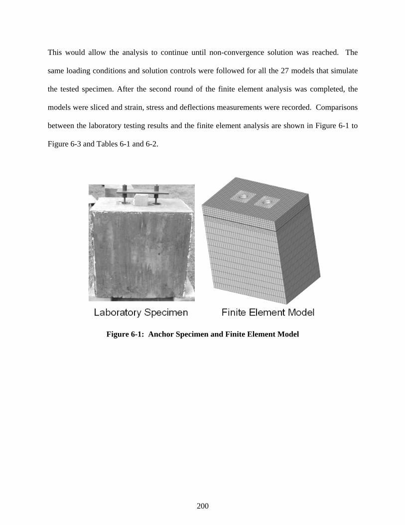
200
This would allow the analysis to continue until non-convergence solution was reached. The
same loading conditions and solution controls were followed for all the 27 models that simulate
the tested specimen. After the second round of the finite element analysis was completed, the
models were sliced and strain, stress and deflections measurements were recorded. Comparisons
between the laboratory testing results and the finite element analysis are shown in Figure 6-1 to
Figure 6-3 and Tables 6-1 and 6-2.
Figure 6-1: Anchor Specimen and Finite Element Model

201
Table 6-1: Comparison between Test and FEA results for S1 Specimens
Embedded Strain Gauges (at 80% of the max load)
Specimen Strain Type
Failure Load (kips)
Deflection (in)
Emb 1 (� strain)
Emb 2 (� strain)
Emb 3 (� strain)
Emb 4 (� strain)
Test 628 0.509 -205 112 158 96.4 S1-1-None/Y/Y FEM 600 0.485 -170 120 146 110 Test 795 0.530 - 121 - 740 S1-2- Dramix/N/N FEM 600 0.505 - 120 - 270 Test 866 0.594 - 313 385 -635 S1-3-Dramix/Y/N FEM 600 0.500 - 210 255 -400 Test 999 0.721 -407 - 262 -229 S1-4-Dramix/N/Y FEM 600 0.495 -380 - 240 -186 Test 1000 0.651 - 224 208 - S1-5-Dramix/0.5/0.6 FEM 600 0.485 - 190 180 - Test 600 0.406 - 82 124 - S1-6-Helix/N/N FEM 600 0.505 - 120 170 - Test 677 0.524 - 82 91 - S1-7-Helix/Y/N FEM 600 0.500 - 126 136 - Test 917 0.619 - 112 108 - S1-8-Helix/N/Y FEM 600 0.495 - 120 160 - Test 869 0.556 - 140 174 - S1-9-Helix/0.5/0.6 FEM 600 0.485 - 120 160 - Test 841 0.549 - 85 283 - S1-10-Novomesh/N/N FEM 600 0.505 - 120 160 - Test 720 0.566 - 458 38 - S1-11-Novomesh/Y/N FEM 600 0.500 - 120 160 - Test 734 0.501 - -193 96 - S1-13- Novomesh/0.5/0.6
FEM 600 0.485 - 120 160 - Test 996 0.684 - 38 83 - S1-14- None/0.5/0.6 FEM 600 0.485 - 80 120 -

202
Table 6-2: Comparison between Test and FEA results for S2 Specimens
Embedded Strain Gauges (at 80% of the max load)
Specimen Strain Type
Failure Load (kips)
Deflection (in)
Emb 1 (� strain)
Emb 2 (� strain)
Emb 3 (� strain)
Emb 4 (� strain)
Test 723 0.550 62 - 158 - S2-1-None/Y/Y FEM 600 0.485 80 - 160 - Test 557 0.434 58 - 100 - S2-2- Dramix/N/N FEM 600 0.505 86 - 170 - Test 628 0.475 100 - 159 S2-3-Dramix/Y/N FEM 600 0.500 120 - 160 - Test 674 0.539 34 - 200 - S2-4-Dramix/N/Y FEM 600 0.495 60 - 170 - Test 666 0.594 109 - 124 - S2-5-Dramix/0.5/0.6 FEM 600 0.485 120 - 140 - Test 568 0.480 17 - 165 - S2-6-Helix/N/N FEM 600 0.505 60 - 140 - Test 691 0.503 -15 - 98 - S2-7-Helix/Y/N FEM 600 0.500 60 - 120 - Test 748 0.504 62 - 120 - S2-8-Helix/N/Y FEM 600 0.495 80 - 120 - Test 753 0.650 39 - 200 - S2-9-Helix/0.5/0.6 FEM 600 0.485 60 - 160 - Test 654 0.475 78 - 124 - S2-10-Novomesh/N/N FEM 600 0.505 60 - 120 - Test 570 0.458 53 - 160 - S2-11-Novomesh/Y/N FEM 600 0.500 60 - 120 - Test 750 0.538 16 - 264 - S2-12-Novomesh/N/Y FEM 600 0.495 60 - 180 - Test 753 0.595 71 - 194 - S2-13-Novomesh/0.5/0.6 FEM 600 0.485 80 - 140- - Test 646 0.570 239 186 143 280 S2-14-None/0.5/0.6 FEM 600 0.485 180 160 120 220

203
Tables 6-1 and 6-2 show that the finite element models sustained loads less that those
encountered in the laboratory tests on anchor specimens. The maximum load in the lab was
1000 kips for S1-5 with Dramix steel fiber and 50% of the spiral reinforcement and 60% of the
ties. The loading capacity for the equivalent FE model was 640 kips. In the second set of
laboratory specimen, the loading capacity of S2-4 was 674 kips. On the other hand, the loading
capacity of S1-1 with full reinforcement and no fibers was 628 kips and the equivalent FE model
was 600 kips. For S2-1, the loading capacity was 723 kips. It was noticed that the cracking
pattern of the S1-1 and S2-1 specimens were similar to those obtained from finite element model
(Figure 6-2).
Figure 6-2: Cracking From Lab Testing and Finite Element Analysis

204
Strain measurements from laboratory testing were also compared with those obtained from the
FEA (Figure 6-3). Tables 6-1 and 6-2 presented strain measurements from embedded gauges in
all the specimens. Since compressive and tensile strains are very high at failure especially when
cracking or crushing occurred at the gauges locations, it was decided to present measurements at
loading levels less than the failure loads. This was also true for the finite element models.
Therefore, it was decided to record strain values for the load steps preceding the failure loads.
Figure 6-3 shows the strain value of the top gauge in S1-1. The Test measurements showed a
value of 237 microstrain (compression) and the FE model resulted in 274 microstrain
(compression).
In general, stress and strain results obtained from the first round of finite element analysis on a
typical bridge segment and from the laboratory testing program on block specimens with two
anchors were comparable. Further validation from the second round of finite element analysis
after laboratory testing confirmed this conclusion. Strain measurements from lab testing were
comparable to those obtained from the finite element models. Deflections from laboratory tests
were mostly higher than those obtained from finite element analysis (Figure 6-4). The reasons
for higher deflections in test specimens were the type of bearing pad underneath the specimens.
At on test a rubber pad was used and then it was replaced by a sand box. Additionally, the initial
applied load on the anchors caused some deflections before the two actuators’ loads were fully
transferred to a specimen. To pass the setting deflections, measurements were taken at the first
inflection point of the load-deformations curve. In most of the cases the setting deflections
ranged between 0.15 to 0.2 in and were subtracted from the total deflection of the specimens.

205
Figure 6-3: Strain Values From Laboratory Testing and Finite Element Analysis
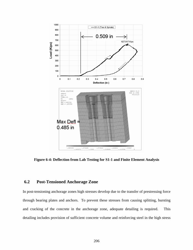
206
Figure 6-4: Deflection from Lab Testing for S1-1 and Finite Element Analysis
6.2 Post-Tensioned Anchorage Zone
In post-tensioning anchorage zones high stresses develop due to the transfer of prestressing force
through bearing plates and anchors. To prevent these stresses from causing splitting, bursting
and cracking of the concrete in the anchorage zone, adequate detailing is required. This
detailing includes provision of sufficient concrete volume and reinforcing steel in the high stress
207
region. Design specifications, anchorage devices and systems, and design experience are
important elements for successfully designing and detailing anchorage zones.
The 2007 AASHTO LRFD Bridge Design Specifications provides recommendations and
guidelines for post-tensioned anchorage zones in Section 5.10.9. In 1994, researchers at the
University of Texas proposed anchorage design specifications for AASHTO as requested
through the National Cooperative Highway Research Program (Breen et al, 1994). The current
AASHTO specification for post-tensioning anchorage zones is based upon the work of Breen et
al. AASHTO states that “for anchorage zones at the end of a segment, the transverse dimensions
may be taken as the depth and width of the section but not larger than the longitudinal dimension
of the component or segment.” The longitudinal dimension of the anchorage zone shall be
greater than or equal to the larger of the transverse dimensions but not greater than 1.5 times this
dimension. In section 5.10.9.2, AASHTO identifies two sections in the anchorage zone, the
general zone and the local zone. The local zone is the region of high compressive stresses
immediately ahead of the anchorage device. The general zone is the remainder of the anchorage
zone and contains the region where the tensile stresses develop as a result of the tendon force
spreading across the section. The Engineer of Record is responsible for the design of the
anchorage zone. Section 5.9.10.9.3 of the AASHTO code lists three methods that may be used
to design the general zone: 1. strut-and-tie models, 2. refined elastic analyses, or 3. other
approximate methods.

208
6.3 Strut-And-Tie Method
Using the AASHTO Guidelines of Section 5.10.9.4 of the code, a strut-and-tie model was made
for the anchorage specimen. The model assumes approximately a 45 degree angle for the
compression struts. By assuming that the maximum bursting force occurs approximately in the
middle of the anchorage zone (for the distance measured along the length of the tendon) and
considering two dimensional approximations, the bursting forces (total tie forces) are computed
for the cross-sectional dimensions of the anchorage block. As shown in the Table 6-3, the
maximum tensile bursting force occurs along the widest cross-sectional dimension (width =
29.5”). The maximum tensile force varies with the magnitude of the applied load (which
simulates the post-tensioning force). Based upon the anchor block geometry and the maximum
applied load of 1000.36 kips, Specimen S1-5 has a maximum computed tie force, bursting force,
of 138.44 kips.
Table 6-4 presents strut-and-tie calculations for Specimen S1-1 for various strut angles relative
to the load surface. As shown in the table, as the angle of the strut with respect to the bearing
surface increases, the magnitude of the bursting force decreases and the distance of the force
away for the load surface increases. Table 6-5, Table 6-6, and Table 6-7 show strut-and-tie
calculations for different strut angles for anchorage test specimens S1-5, S2-1, and S2-13,
respectively. Similar calculations were done for all of the other anchorage test specimens.

209
Table 6-3: Strut And Tie Two Dimensional Approximation For Bursting Force
Strut & Tie (Truss Calculations) : Two - 2D Approximations Added Together
Specimen Specimen MembersID Total West East 9+11 10+12 1 2 3 4 5 6 7 8 9 10 11 12 13 14 15 16
Load Actuator Actuator Tie Total Tie Total Tie Tie Tie Tie(K) P1 (K) P2 (K) (Kips) (Kips)
S1 Specimens LONG SHORT LONG SHORT LONG SHORT1 S1-1 627.92 314.93 312.99 86.82 67.28 43.41 33.53 43.41 33.74 175.44 174.52 174.52 175.44 43.41 33.53 43.41 33.74 157.32 156.84 156.84 157.322 S1-2 794.00 389.24 404.75 108.77 85.07 54.39 43.37 54.39 41.70 218.35 225.69 225.69 218.35 54.39 43.37 54.39 41.70 195.77 199.65 199.65 195.773 S1-3 865.33 428.84 436.49 119.07 92.71 59.53 46.77 59.53 45.95 239.77 243.39 243.39 239.77 59.53 46.77 59.53 45.95 214.99 216.90 216.90 214.994 S1-4 999.23 500.18 499.05 138.05 107.06 69.03 53.47 69.03 53.59 278.80 278.27 278.27 278.80 69.03 53.47 69.03 53.59 250.01 249.73 249.73 250.015 S1-5 1000.36 502.79 497.56 138.44 107.18 69.22 53.31 69.22 53.87 279.92 277.44 277.44 279.92 69.22 53.31 69.22 53.87 251.01 249.70 249.70 251.016 S1-6 599.94 293.80 306.15 82.15 64.28 41.08 32.80 41.08 31.48 164.86 170.71 170.71 164.86 41.08 32.80 41.08 31.48 147.81 150.90 150.90 147.817 S1-7 676.74 337.42 339.32 93.35 72.51 46.67 36.36 46.67 36.15 188.31 189.20 189.20 188.31 46.67 36.36 46.67 36.15 168.85 169.32 169.32 168.858 S1-8 916.70 460.24 456.45 126.81 98.22 63.40 48.91 63.40 49.31 256.31 254.52 254.52 256.31 63.40 48.91 63.40 49.31 229.84 228.89 228.89 229.849 S1-9 869.23 436.39 432.84 120.24 93.13 60.12 46.38 60.12 46.76 243.03 241.35 241.35 243.03 60.12 46.38 60.12 46.76 217.93 217.04 217.04 217.93
10 S1-10 827.22 403.18 424.04 113.06 88.63 56.53 45.43 56.53 43.20 226.58 236.44 236.44 226.58 56.53 45.43 56.53 43.20 203.13 208.35 208.35 203.1311 S1-11 704.80 349.84 354.96 97.04 75.51 48.52 38.03 48.52 37.48 195.50 197.93 197.93 195.50 48.52 38.03 48.52 37.48 175.30 176.58 176.58 175.3012 S1-13 732.53 365.46 367.07 101.07 78.49 50.53 39.33 50.53 39.16 203.92 204.68 204.68 203.92 50.53 39.33 50.53 39.16 182.85 183.25 183.25 182.8513 S1-14 995.59 496.17 499.43 137.30 106.67 68.65 53.51 68.65 53.16 276.94 278.48 278.48 276.94 68.65 53.51 68.65 53.16 248.32 249.14 249.14 248.32
S2 Specimens 14 S2-1 723.25 365.94 357.31 100.36 77.49 50.18 38.28 50.18 39.21 203.32 199.24 199.24 203.32 50.18 38.28 50.18 39.21 182.33 180.17 180.17 182.3315 S2-2 552.87 273.10 279.77 75.97 59.24 37.99 29.97 37.99 29.26 152.85 156.00 156.00 152.85 37.99 29.97 37.99 29.26 137.04 138.71 138.71 137.0416 S2-3 626.89 316.41 310.48 86.90 67.17 43.45 33.27 43.45 33.90 175.93 173.12 173.12 175.93 43.45 33.27 43.45 33.90 157.76 156.28 156.28 157.7617 S2-4 673.86 332.58 341.29 92.57 72.20 46.28 36.57 46.28 35.63 186.18 190.30 190.30 186.18 46.28 36.57 46.28 35.63 166.93 169.11 169.11 166.9318 S2-5 665.56 323.08 342.47 90.82 71.31 45.41 36.69 45.41 34.62 181.79 190.96 190.96 181.79 45.41 36.69 45.41 34.62 162.98 167.82 167.82 162.9819 S2-6 566.51 280.34 286.17 77.90 60.70 38.95 30.66 38.95 30.04 156.81 159.57 159.57 156.81 38.95 30.66 38.95 30.04 140.60 142.06 142.06 140.6020 S2-7 691.14 347.09 344.05 95.61 74.05 47.81 36.86 47.81 37.19 193.28 191.84 191.84 193.28 47.81 36.86 47.81 37.19 173.32 172.56 172.56 173.3221 S2-8 747.70 371.67 376.03 103.01 80.11 51.50 40.29 51.50 39.82 207.61 209.68 209.68 207.61 51.50 40.29 51.50 39.82 186.16 187.25 187.25 186.1622 S2-9 752.57 370.22 382.36 103.24 80.63 51.62 40.97 51.62 39.67 207.46 213.20 213.20 207.46 51.62 40.97 51.62 39.67 186.01 189.04 189.04 186.0123 S2-10 653.63 327.53 326.10 90.34 70.03 45.17 34.94 45.17 35.09 182.51 181.83 181.83 182.51 45.17 34.94 45.17 35.09 163.66 163.30 163.30 163.6624 S2-11 569.55 285.02 284.53 78.68 61.02 39.34 30.49 39.34 30.54 158.89 158.65 158.65 158.89 39.34 30.49 39.34 30.54 142.48 142.35 142.35 142.4825 S2-12 749.99 374.45 375.53 103.51 80.36 51.75 40.24 51.75 40.12 208.89 209.40 209.40 208.89 51.75 40.24 51.75 40.12 187.31 187.58 187.58 187.3126 S2-13 752.68 370.37 382.32 103.27 80.64 51.63 40.96 51.63 39.68 207.53 213.18 213.18 207.53 51.63 40.96 51.63 39.68 186.07 189.05 189.05 186.0727 S2-14 645.77 326.27 319.50 89.56 69.19 44.78 34.23 44.78 34.96 181.36 178.15 178.15 181.36 44.78 34.23 44.78 34.96 162.64 160.94 160.94 162.64
Table 6-4: Strut And Tie Bursting Forces For Specimen S1-1 Strut & Tie (Truss Calculations) : Two - 2D Approximations Added Together
Specimen Specimen # ID Total West East 9+11 10+12
Load Actuator Actuator Tie Total Tie Total 19.5 29.5(K) P1 (K) P2 (K) (Kips) (Kips) SHORT Degrees Radians LONG Degrees Radians
X H1 X/H1 Theta1 Theta1 X H2 X/H2 Theta2 Theta21 S1-1 627.92 314.93 312.99 1571.77 1217.94 0.725 19.5 0.04 7.34 0.13 0.725 29.5 0.02 5.71 0.101 S1-1 627.92 314.93 312.99 930.23 720.82 1.225 19.5 0.06 12.29 0.21 1.225 29.5 0.04 9.59 0.171 S1-1 627.92 314.93 312.99 785.88 608.97 1.450 19.5 0.07 14.45 0.25 1.450 29.5 0.05 11.31 0.201 S1-1 627.92 314.93 312.99 523.92 405.98 2.175 19.5 0.11 21.14 0.37 2.175 29.5 0.07 16.70 0.291 S1-1 627.92 314.93 312.99 465.12 360.41 2.450 19.5 0.13 23.54 0.41 2.450 29.5 0.08 18.67 0.331 S1-1 627.92 314.93 312.99 392.94 304.49 2.900 19.5 0.15 27.27 0.48 2.900 29.5 0.10 21.80 0.381 S1-1 627.92 314.93 312.99 314.35 243.59 3.625 19.5 0.19 32.80 0.57 3.625 29.5 0.12 26.57 0.461 S1-1 627.92 314.93 312.99 310.08 240.27 3.675 19.5 0.19 33.16 0.58 3.675 29.5 0.12 26.88 0.471 S1-1 627.92 314.93 312.99 261.96 202.99 4.350 19.5 0.22 37.72 0.66 4.350 29.5 0.15 30.96 0.541 S1-1 627.92 314.93 312.99 232.56 180.21 4.900 19.5 0.25 41.06 0.72 4.900 29.5 0.17 34.05 0.591 S1-1 627.92 314.93 312.99 224.54 173.99 5.075 19.5 0.26 42.06 0.73 5.075 29.5 0.17 34.99 0.611 S1-1 627.92 314.93 312.99 196.47 152.24 5.800 19.5 0.30 45.88 0.80 5.800 29.5 0.20 38.66 0.671 S1-1 627.92 314.93 312.99 186.05 144.16 6.125 19.5 0.31 47.44 0.83 6.125 29.5 0.21 40.19 0.701 S1-1 627.92 314.93 312.99 174.64 135.33 6.525 19.5 0.33 49.24 0.86 6.525 29.5 0.22 41.99 0.731 S1-1 627.92 314.93 312.99 166.91 129.33 6.827 19.5 0.35 50.52 0.88 6.827 29.5 0.23 43.28 0.761 S1-1 627.92 314.93 312.99 157.18 121.79 7.250 19.5 0.37 52.19 0.91 7.250 29.5 0.25 45.00 0.791 S1-1 627.92 314.93 312.99 155.04 120.14 7.350 19.5 0.38 52.57 0.92 7.350 29.5 0.25 45.39 0.791 S1-1 627.92 314.93 312.99 146.70 113.68 7.768 19.5 0.40 54.09 0.94 7.768 29.5 0.26 46.97 0.821 S1-1 627.92 314.93 312.99 132.89 102.97 8.575 19.5 0.44 56.74 0.99 8.575 29.5 0.29 49.79 0.871 S1-1 627.92 314.93 312.99 116.88 90.57 9.750 19.5 0.50 60.02 1.05 9.750 29.5 0.33 53.37 0.931 S1-1 627.92 314.93 312.99 116.28 90.10 9.800 19.5 0.50 60.15 1.05 9.800 29.5 0.33 53.51 0.931 S1-1 627.92 314.93 312.99 103.36 80.09 11.025 19.5 0.57 62.97 1.10 11.025 29.5 0.37 56.67 0.991 S1-1 627.92 314.93 312.99 98.78 76.54 11.536 19.5 0.59 64.01 1.12 11.536 29.5 0.39 57.85 1.011 S1-1 627.92 314.93 312.99 93.02 72.08 12.250 19.5 0.63 65.34 1.14 12.250 29.5 0.42 59.38 1.041 S1-1 627.92 314.93 312.99 86.82 67.28 13.125 19.5 0.67 66.80 1.17 13.125 29.5 0.44 61.08 1.071 S1-1 627.92 314.93 312.99 77.26 59.87 14.750 19.5 0.76 69.13 1.21 14.750 29.5 0.50 63.82 1.11

210
Table 6-5: Strut And Tie Bursting Forces For Specimen S1-5
Strut & Tie (Truss Calculations) : Two - 2D Approximations Added Together
Specimen Specimen # ID Total West East 9+11 10+12
Load Actuator Actuator Tie Total Tie Total 19.5 29.5(K) P1 (K) P2 (K) (Kips) (Kips) SHORT Degrees Radians LONG Degrees Radians
X H1 X/H1 Theta1 Theta1 X H2 X/H2 Theta2 Theta25 S1-5 1000.36 502.79 497.56 2506.23 1940.35 0.725 19.5 0.04 7.34 0.13 0.725 29.5 0.02 5.71 0.105 S1-5 1000.36 502.79 497.56 1483.28 1148.37 1.225 19.5 0.06 12.29 0.21 1.225 29.5 0.04 9.59 0.175 S1-5 1000.36 502.79 497.56 1253.12 970.17 1.450 19.5 0.07 14.45 0.25 1.450 29.5 0.05 11.31 0.205 S1-5 1000.36 502.79 497.56 835.41 646.78 2.175 19.5 0.11 21.14 0.37 2.175 29.5 0.07 16.70 0.295 S1-5 1000.36 502.79 497.56 741.64 574.18 2.450 19.5 0.13 23.54 0.41 2.450 29.5 0.08 18.67 0.335 S1-5 1000.36 502.79 497.56 626.56 485.09 2.900 19.5 0.15 27.27 0.48 2.900 29.5 0.10 21.80 0.385 S1-5 1000.36 502.79 497.56 501.25 388.07 3.625 19.5 0.19 32.80 0.57 3.625 29.5 0.12 26.57 0.465 S1-5 1000.36 502.79 497.56 494.43 382.79 3.675 19.5 0.19 33.16 0.58 3.675 29.5 0.12 26.88 0.475 S1-5 1000.36 502.79 497.56 417.71 323.39 4.350 19.5 0.22 37.72 0.66 4.350 29.5 0.15 30.96 0.545 S1-5 1000.36 502.79 497.56 370.82 287.09 4.900 19.5 0.25 41.06 0.72 4.900 29.5 0.17 34.05 0.595 S1-5 1000.36 502.79 497.56 358.03 277.19 5.075 19.5 0.26 42.06 0.73 5.075 29.5 0.17 34.99 0.615 S1-5 1000.36 502.79 497.56 313.28 242.54 5.800 19.5 0.30 45.88 0.80 5.800 29.5 0.20 38.66 0.675 S1-5 1000.36 502.79 497.56 296.66 229.67 6.125 19.5 0.31 47.44 0.83 6.125 29.5 0.21 40.19 0.705 S1-5 1000.36 502.79 497.56 278.47 215.59 6.525 19.5 0.33 49.24 0.86 6.525 29.5 0.22 41.99 0.735 S1-5 1000.36 502.79 497.56 266.14 206.05 6.827 19.5 0.35 50.52 0.88 6.827 29.5 0.23 43.28 0.765 S1-5 1000.36 502.79 497.56 250.62 194.03 7.250 19.5 0.37 52.19 0.91 7.250 29.5 0.25 45.00 0.795 S1-5 1000.36 502.79 497.56 247.21 191.39 7.350 19.5 0.38 52.57 0.92 7.350 29.5 0.25 45.39 0.795 S1-5 1000.36 502.79 497.56 233.92 181.10 7.768 19.5 0.40 54.09 0.94 7.768 29.5 0.26 46.97 0.825 S1-5 1000.36 502.79 497.56 211.90 164.05 8.575 19.5 0.44 56.74 0.99 8.575 29.5 0.29 49.79 0.875 S1-5 1000.36 502.79 497.56 186.36 144.28 9.750 19.5 0.50 60.02 1.05 9.750 29.5 0.33 53.37 0.935 S1-5 1000.36 502.79 497.56 185.41 143.55 9.800 19.5 0.50 60.15 1.05 9.800 29.5 0.33 53.51 0.935 S1-5 1000.36 502.79 497.56 164.81 127.60 11.025 19.5 0.57 62.97 1.10 11.025 29.5 0.37 56.67 0.995 S1-5 1000.36 502.79 497.56 157.51 121.95 11.536 19.5 0.59 64.01 1.12 11.536 29.5 0.39 57.85 1.015 S1-5 1000.36 502.79 497.56 148.33 114.84 12.250 19.5 0.63 65.34 1.14 12.250 29.5 0.42 59.38 1.045 S1-5 1000.36 502.79 497.56 138.44 107.18 13.125 19.5 0.67 66.80 1.17 13.125 29.5 0.44 61.08 1.075 S1-5 1000.36 502.79 497.56 123.19 95.37 14.750 19.5 0.76 69.13 1.21 14.750 29.5 0.50 63.82 1.11
Table 6-6: Strut And Tie Bursting Forces For Specimen S2-1 Strut & Tie (Truss Calculations) : Two - 2D Approximations Added Together
Specimen Specimen # ID Total West East 9+11 10+12
Load Actuator Actuator Tie Total Tie Total 19.5 29.5(K) P1 (K) P2 (K) (Kips) (Kips) SHORT Degrees Radians LONG Degrees Radians
X H1 X/H1 Theta1 Theta1 X H2 X/H2 Theta2 Theta214 S2-1 723.25 365.94 357.31 1816.93 1402.85 0.725 19.5 0.04 7.34 0.13 0.725 29.5 0.02 5.71 0.1014 S2-1 723.25 365.94 357.31 1075.32 830.26 1.225 19.5 0.06 12.29 0.21 1.225 29.5 0.04 9.59 0.1714 S2-1 723.25 365.94 357.31 908.46 701.43 1.450 19.5 0.07 14.45 0.25 1.450 29.5 0.05 11.31 0.2014 S2-1 723.25 365.94 357.31 605.64 467.62 2.175 19.5 0.11 21.14 0.37 2.175 29.5 0.07 16.70 0.2914 S2-1 723.25 365.94 357.31 537.66 415.13 2.450 19.5 0.13 23.54 0.41 2.450 29.5 0.08 18.67 0.3314 S2-1 723.25 365.94 357.31 454.23 350.71 2.900 19.5 0.15 27.27 0.48 2.900 29.5 0.10 21.80 0.3814 S2-1 723.25 365.94 357.31 363.39 280.57 3.625 19.5 0.19 32.80 0.57 3.625 29.5 0.12 26.57 0.4614 S2-1 723.25 365.94 357.31 358.44 276.75 3.675 19.5 0.19 33.16 0.58 3.675 29.5 0.12 26.88 0.4714 S2-1 723.25 365.94 357.31 302.82 233.81 4.350 19.5 0.22 37.72 0.66 4.350 29.5 0.15 30.96 0.5414 S2-1 723.25 365.94 357.31 268.83 207.57 4.900 19.5 0.25 41.06 0.72 4.900 29.5 0.17 34.05 0.5914 S2-1 723.25 365.94 357.31 259.56 200.41 5.075 19.5 0.26 42.06 0.73 5.075 29.5 0.17 34.99 0.6114 S2-1 723.25 365.94 357.31 227.12 175.36 5.800 19.5 0.30 45.88 0.80 5.800 29.5 0.20 38.66 0.6714 S2-1 723.25 365.94 357.31 215.06 166.05 6.125 19.5 0.31 47.44 0.83 6.125 29.5 0.21 40.19 0.7014 S2-1 723.25 365.94 357.31 201.88 155.87 6.525 19.5 0.33 49.24 0.86 6.525 29.5 0.22 41.99 0.7314 S2-1 723.25 365.94 357.31 192.94 148.97 6.827 19.5 0.35 50.52 0.88 6.827 29.5 0.23 43.28 0.7614 S2-1 723.25 365.94 357.31 181.69 140.29 7.250 19.5 0.37 52.19 0.91 7.250 29.5 0.25 45.00 0.7914 S2-1 723.25 365.94 357.31 179.22 138.38 7.350 19.5 0.38 52.57 0.92 7.350 29.5 0.25 45.39 0.7914 S2-1 723.25 365.94 357.31 169.58 130.93 7.768 19.5 0.40 54.09 0.94 7.768 29.5 0.26 46.97 0.8214 S2-1 723.25 365.94 357.31 153.62 118.61 8.575 19.5 0.44 56.74 0.99 8.575 29.5 0.29 49.79 0.8714 S2-1 723.25 365.94 357.31 135.10 104.31 9.750 19.5 0.50 60.02 1.05 9.750 29.5 0.33 53.37 0.9314 S2-1 723.25 365.94 357.31 134.42 103.78 9.800 19.5 0.50 60.15 1.05 9.800 29.5 0.33 53.51 0.9314 S2-1 723.25 365.94 357.31 119.48 92.25 11.025 19.5 0.57 62.97 1.10 11.025 29.5 0.37 56.67 0.9914 S2-1 723.25 365.94 357.31 114.19 88.17 11.536 19.5 0.59 64.01 1.12 11.536 29.5 0.39 57.85 1.0114 S2-1 723.25 365.94 357.31 107.53 83.03 12.250 19.5 0.63 65.34 1.14 12.250 29.5 0.42 59.38 1.0414 S2-1 723.25 365.94 357.31 100.36 77.49 13.125 19.5 0.67 66.80 1.17 13.125 29.5 0.44 61.08 1.0714 S2-1 723.25 365.94 357.31 89.31 68.95 14.750 19.5 0.76 69.13 1.21 14.750 29.5 0.50 63.82 1.11
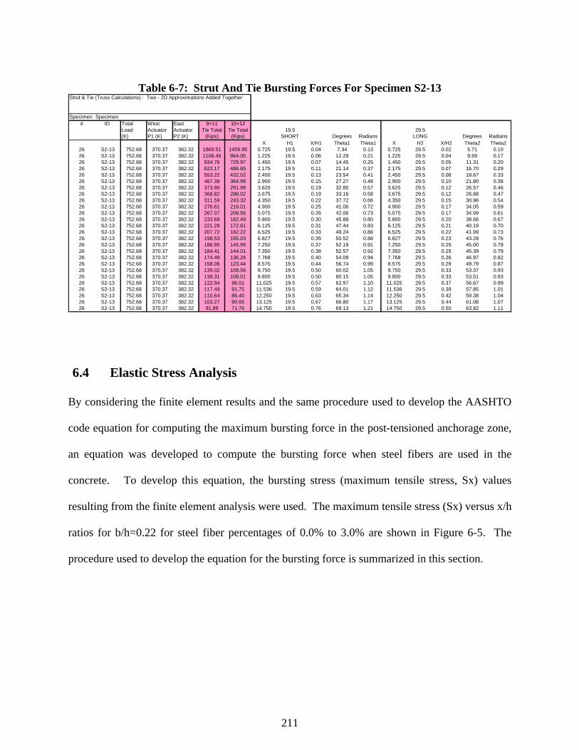
211
Table 6-7: Strut And Tie Bursting Forces For Specimen S2-13
Strut & Tie (Truss Calculations) : Two - 2D Approximations Added Together
Specimen Specimen # ID Total West East 9+11 10+12
Load Actuator Actuator Tie Total Tie Total 19.5 29.5(K) P1 (K) P2 (K) (Kips) (Kips) SHORT Degrees Radians LONG Degrees Radians
X H1 X/H1 Theta1 Theta1 X H2 X/H2 Theta2 Theta226 S2-13 752.68 370.37 382.32 1869.51 1459.95 0.725 19.5 0.04 7.34 0.13 0.725 29.5 0.02 5.71 0.1026 S2-13 752.68 370.37 382.32 1106.45 864.05 1.225 19.5 0.06 12.29 0.21 1.225 29.5 0.04 9.59 0.1726 S2-13 752.68 370.37 382.32 934.76 729.97 1.450 19.5 0.07 14.45 0.25 1.450 29.5 0.05 11.31 0.2026 S2-13 752.68 370.37 382.32 623.17 486.65 2.175 19.5 0.11 21.14 0.37 2.175 29.5 0.07 16.70 0.2926 S2-13 752.68 370.37 382.32 553.22 432.02 2.450 19.5 0.13 23.54 0.41 2.450 29.5 0.08 18.67 0.3326 S2-13 752.68 370.37 382.32 467.38 364.99 2.900 19.5 0.15 27.27 0.48 2.900 29.5 0.10 21.80 0.3826 S2-13 752.68 370.37 382.32 373.90 291.99 3.625 19.5 0.19 32.80 0.57 3.625 29.5 0.12 26.57 0.4626 S2-13 752.68 370.37 382.32 368.82 288.02 3.675 19.5 0.19 33.16 0.58 3.675 29.5 0.12 26.88 0.4726 S2-13 752.68 370.37 382.32 311.59 243.32 4.350 19.5 0.22 37.72 0.66 4.350 29.5 0.15 30.96 0.5426 S2-13 752.68 370.37 382.32 276.61 216.01 4.900 19.5 0.25 41.06 0.72 4.900 29.5 0.17 34.05 0.5926 S2-13 752.68 370.37 382.32 267.07 208.56 5.075 19.5 0.26 42.06 0.73 5.075 29.5 0.17 34.99 0.6126 S2-13 752.68 370.37 382.32 233.69 182.49 5.800 19.5 0.30 45.88 0.80 5.800 29.5 0.20 38.66 0.6726 S2-13 752.68 370.37 382.32 221.29 172.81 6.125 19.5 0.31 47.44 0.83 6.125 29.5 0.21 40.19 0.7026 S2-13 752.68 370.37 382.32 207.72 162.22 6.525 19.5 0.33 49.24 0.86 6.525 29.5 0.22 41.99 0.7326 S2-13 752.68 370.37 382.32 198.53 155.03 6.827 19.5 0.35 50.52 0.88 6.827 29.5 0.23 43.28 0.7626 S2-13 752.68 370.37 382.32 186.95 145.99 7.250 19.5 0.37 52.19 0.91 7.250 29.5 0.25 45.00 0.7926 S2-13 752.68 370.37 382.32 184.41 144.01 7.350 19.5 0.38 52.57 0.92 7.350 29.5 0.25 45.39 0.7926 S2-13 752.68 370.37 382.32 174.49 136.26 7.768 19.5 0.40 54.09 0.94 7.768 29.5 0.26 46.97 0.8226 S2-13 752.68 370.37 382.32 158.06 123.44 8.575 19.5 0.44 56.74 0.99 8.575 29.5 0.29 49.79 0.8726 S2-13 752.68 370.37 382.32 139.02 108.56 9.750 19.5 0.50 60.02 1.05 9.750 29.5 0.33 53.37 0.9326 S2-13 752.68 370.37 382.32 138.31 108.01 9.800 19.5 0.50 60.15 1.05 9.800 29.5 0.33 53.51 0.9326 S2-13 752.68 370.37 382.32 122.94 96.01 11.025 19.5 0.57 62.97 1.10 11.025 29.5 0.37 56.67 0.9926 S2-13 752.68 370.37 382.32 117.49 91.75 11.536 19.5 0.59 64.01 1.12 11.536 29.5 0.39 57.85 1.0126 S2-13 752.68 370.37 382.32 110.64 86.40 12.250 19.5 0.63 65.34 1.14 12.250 29.5 0.42 59.38 1.0426 S2-13 752.68 370.37 382.32 103.27 80.65 13.125 19.5 0.67 66.80 1.17 13.125 29.5 0.44 61.08 1.0726 S2-13 752.68 370.37 382.32 91.89 71.76 14.750 19.5 0.76 69.13 1.21 14.750 29.5 0.50 63.82 1.11
6.4 Elastic Stress Analysis
By considering the finite element results and the same procedure used to develop the AASHTO
code equation for computing the maximum bursting force in the post-tensioned anchorage zone,
an equation was developed to compute the bursting force when steel fibers are used in the
concrete. To develop this equation, the bursting stress (maximum tensile stress, Sx) values
resulting from the finite element analysis were used. The maximum tensile stress (Sx) versus x/h
ratios for b/h=0.22 for steel fiber percentages of 0.0% to 3.0% are shown in Figure 6-5. The
procedure used to develop the equation for the bursting force is summarized in this section.

212
Figure 6-5: Maximum Tensile Stress, Sx, versus h/x for 0.0% To 3.0% Fiber
Using the finite element results, for different fiber percentages (0% to 3.0%), plots were made of
the maximum tensile stress versus distances along the anchorage zone. The maximum tensile
stress (Sx) versus x/h ratios plots for 0.0% to 3.0% steel fibers are shown in Figure 6-6 to Figure
6-10. The b/h ratios ranged from 0.0 to 1.0. The areas under the Sx versus x/h curves for each
percentage of fiber were computed to obtain the bursting force, Tmax. By plotting the bursting
forces (areas under the stress curves) versus b/h for each percentage of fiber, an equation relating
Tmax to b/h was obtained by fitting a line through the plot. See Figure 6-11 to Figure 6-15. Each
of these figures shows an equation for the best fit line to the curve for Tmax. These equations
were used to compute the Tmax values shown in Table 6-8. The bursting force (Tmax) values
computed in Table 6-8 to Table 6-11 are based on a one Kip (1 K) tendon force (unit value).

213
Figure 6-6: Maximum Tensile Stress, Sx, Versus x/h For 0.0% Fiber
Figure 6-7 Maximum Tensile Stress, Sx Versus x/h For 0.5% Fiber

214
Figure 6-8: Maximum Tensile Stress, Sx, Versus x/h For 1.0% Fiber
Figure 6-9: Maximum Tensile Stress, Sx, Versus x/h For 2.0% Fiber
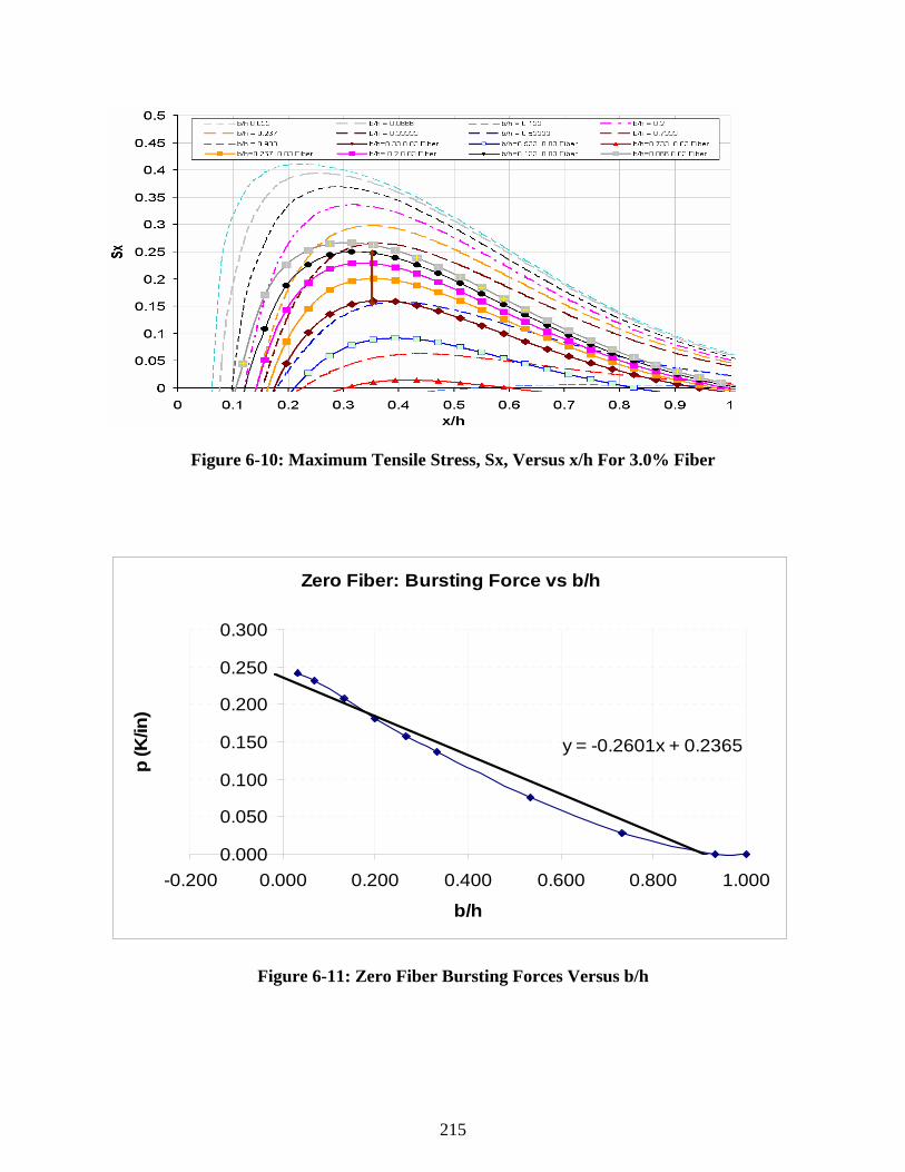
215
Figure 6-10: Maximum Tensile Stress, Sx, Versus x/h For 3.0% Fiber
Zero Fiber: Bursting Force vs b/h
y = -0.2601x + 0.2365
0.000
0.050
0.100
0.150
0.200
0.250
0.300
-0.200 0.000 0.200 0.400 0.600 0.800 1.000
b/h
p (K
/in)
Figure 6-11: Zero Fiber Bursting Forces Versus b/h

216
0.5% Fiber: Bursting Force vs b/h
y = -0.2307x + 0.2077
0.000
0.050
0.100
0.150
0.200
0.250
0.000 0.100 0.200 0.300 0.400 0.500 0.600 0.700 0.800 0.900 1.000
b/h
P (K
)
Figure 6-12: 0.5% Fiber Bursting Forces Versus b/h
1.0% Fiber: Bursting Force vs b/h
y = -0.2166x + 0.1905
0.000
0.050
0.100
0.150
0.200
0.250
0.000 0.100 0.200 0.300 0.400 0.500 0.600 0.700 0.800 0.900 1.000
b/h
P (K
)
Figure 6-13: 1.0% Fiber Bursting Forces Versus b/h

217
2.0% Fiber: Bursting Force vs b/h
y = -0.1818x + 0.1576
0.000
0.050
0.100
0.150
0.200
0.250
0.000 0.100 0.200 0.300 0.400 0.500 0.600 0.700 0.800 0.900 1.000
b/h
P (K
)
Figure 6-14: 2.0% Fiber Bursting Forces Versus b/h
3.0% Fiber: Bursting Force vs b/h
y = -0.1523x + 0.1298
0.000
0.050
0.100
0.150
0.200
0.250
0.000 0.100 0.200 0.300 0.400 0.500 0.600 0.700 0.800 0.900 1.000
b/h
P (K
)
Figure 6-15: 3.0% Fiber Bursting Forces Versus b/h
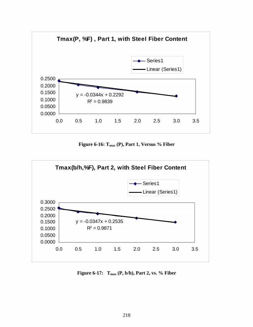
218
Tmax(P, %F) , Part 1, with Steel Fiber Content
y = -0.0344x + 0.2292R2 = 0.9839
0.00000.05000.10000.15000.20000.2500
0.0 0.5 1.0 1.5 2.0 2.5 3.0 3.5
Series1
Linear (Series1)
Figure 6-16: Tmax (P), Part 1, Versus % Fiber
Tmax(b/h,%F), Part 2, with Steel Fiber Content
y = -0.0347x + 0.2535R2 = 0.9871
0.00000.05000.10000.15000.20000.25000.3000
0.0 0.5 1.0 1.5 2.0 2.5 3.0 3.5
Series1
Linear (Series1)
Figure 6-17: Tmax (P, b/h), Part 2, vs. % Fiber

219
% Decrease of Tmax with Steel Fiber Content (b/h=0.333)
y = 0.1372x + 0.1317R2 = 0.9815
0.0%10.0%20.0%30.0%40.0%50.0%60.0%
0.0 0.5 1.0 1.5 2.0 2.5 3.0 3.5
Figure 6-18: Percent Decrease of Tmax with Steel Fiber Content
Next, considering the Tmax equations obtained for each percentage of fiber, the equations were
separated into two parts (Part 1 and Part 2). Plotting the coefficients versus fiber percentages for
Part 1 and getting a best fit line for the curve to this part yields an equation relating Tmax to the
applied compressive load (tendon force, P) and the fiber percentage. Plotting the coefficients
versus fiber percentages for Part 2 and obtaining the best fit line for the curve, yields an equation
relating Tmax to the b/h ratio and the fiber percentage. Then by adding the two equations for Part
1 and Part 2, an equation is obtained which relates Tmax to the applied compressive force (P), the
b/h ratio and the fiber percentage. The full equation (by adding Part 1 and Part 2), is as follows:
Tmax=0.23 P - 0.034 P(%F) – P (0.25) (b/h) + P(0.03) (b/h)(%F) 6-1

220
Using the equation determined for Tmax, the Tmax values can be computed and compared to both
the AASHTO equation Tmax and the Tmax values computed by using the finite element results
(Sx/h versus b/h plots). In Table 6.9, bursting force values are computed for b/h = 0.33 for fiber
percentages ranging from 0.0% (no fiber) to 3.0%. Table 6-9 shows that the Tmax values
computed using the developed equation are on average 0.02% different from the values
computed by determining the area under the curves of the Sx versus b/h plots for b/h = 0.333.
The table also shows that by adding steel fibers in the concrete, the finite element results indicate
that the maximum tensile force developed will be approximately 20% less for 0.5% fibers and
approximately 54.3% less for 3.0% fibers.
By rounding the numbers in the equation to two decimal places, the equation proposed for
computing the bursting force with consideration for both fiber percentage and b/h ratio becomes:
Tmax = 0.23 P [1-1.11(b/h)-0.15(b)+0.15(b/h)(F%)] 6-2
Table 6-10 shows Tmax values computed by the proposed equation for various b/h ratios and fiber
percentages. Table 6-10 and Table 6-11 show comparisons with the Tmax values computed by
the AASHTO equation and the new equation for various b/h ratios and two different equation
coefficients (0.23 and 0.24). As shown by comparing the two tables, if a coefficient equal to
0.24 is used, the bursting forces calculated are more conservative and are almost always greater
than the AASHTO values.

221
Table 6-8: Bursting Forces Comparison If Max b/h=1.0
AASHTO: A(P)(1-b/h) = A(P)-(P)(B)(b/h)= Tmax(P) % % change FEM: A(P)-B(P)(b/h) AASHTO in Tmax
Assume P=1.0 Decrease% Fiber A B b/h Tmax 1/Tmax
AASHTO 0 0.25 0.25 0.033 0.242 4.1 100.0% 0%0.25 0.25 0.067 0.233 4.3 100.0% 0%0.25 0.25 0.133 0.217 4.6 100.0% 0%0.25 0.25 0.200 0.200 5.0 100.0% 0%0.25 0.25 0.267 0.183 5.5 100.0% 0%0.25 0.25 0.333 0.167 6.0 100.0% 0%0.25 0.25 0.533 0.117 8.6 100.0% 0%0.25 0.25 0.733 0.067 15.0 100.0% 0%
FEM 0 0.2365 0.2601 0.033 0.228 4.4 94.3% 5.7%0.2365 0.2601 0.067 0.219 4.6 93.9% 6.1%0.2365 0.2601 0.133 0.202 5.0 93.1% 6.9%0.2365 0.2601 0.200 0.184 5.4 92.2% 7.8%0.2365 0.2601 0.267 0.167 6.0 91.2% 8.8%0.2365 0.2601 0.333 0.150 6.7 89.9% 10.1%0.2365 0.2601 0.533 0.098 10.2 83.8% 16.2%0.2365 0.2601 0.733 0.046 21.8 68.6% 31.4%
FEM 0.5 0.2077 0.2307 0.033 0.200 5.0 82.8% 17.2%0.2077 0.2307 0.067 0.192 5.2 82.4% 17.6%0.2077 0.2307 0.133 0.177 5.7 81.7% 18.3%0.2077 0.2307 0.200 0.162 6.2 80.8% 19.2%0.2077 0.2307 0.267 0.146 6.8 79.7% 20.3%0.2077 0.2307 0.333 0.131 7.6 78.5% 21.5%0.2077 0.2307 0.533 0.085 11.8 72.6% 27.4%0.2077 0.2307 0.733 0.039 26.0 57.8% 42.2%
FEM 1.0 0.1905 0.2166 0.033 0.183 5.5 75.8% 24.2%0.1905 0.2166 0.067 0.176 5.7 75.5% 24.5%0.1905 0.2166 0.133 0.162 6.2 74.6% 25.4%0.1905 0.2166 0.200 0.147 6.8 73.6% 26.4%0.1905 0.2166 0.267 0.133 7.5 72.4% 27.6%0.1905 0.2166 0.333 0.118 8.5 71.0% 29.0%0.1905 0.2166 0.533 0.075 13.3 64.3% 35.7%0.1905 0.2166 0.733 0.032 31.6 47.5% 52.5%
FEM 2.0 0.1576 0.1818 0.033 0.152 6.6 62.7% 37.3%0.1576 0.1818 0.067 0.145 6.9 62.3% 37.7%0.1576 0.1818 0.133 0.133 7.5 61.6% 38.4%0.1576 0.1818 0.200 0.121 8.2 60.6% 39.4%0.1576 0.1818 0.267 0.109 9.2 59.5% 40.5%0.1576 0.1818 0.333 0.097 10.3 58.2% 41.8%0.1576 0.1818 0.533 0.061 16.5 52.0% 48.0%0.1576 0.1818 0.733 0.024 41.2 36.4% 63.6%
FEM 3.0 0.1298 0.1532 0.033 0.125 8.0 51.6% 48.4%0.1298 0.1523 0.067 0.120 8.4 51.3% 48.7%0.1298 0.1523 0.133 0.109 9.1 50.5% 49.5%0.1298 0.1523 0.200 0.099 10.1 49.7% 50.3%0.1298 0.1523 0.267 0.089 11.2 48.6% 51.4%0.1298 0.1523 0.333 0.079 12.7 47.4% 52.6%0.1298 0.1523 0.533 0.049 20.6 41.6% 58.4%0.1298 0.1523 0.733 0.018 55.2 27.2% 72.8%

222
Table 6-9: Tmax Comparison To AASHTO If Max b/h=1.0
FEM Tmax= Part 1-Part 2FEM Tmax= 0.2292P-0.0344P(%F) -P(0.2535(b/h)+P(0.0347(b/h)(%F)
Tmax= 0.2292P[1-1.1060(b/h)-0.1501(%F)+0.1514(b/h)(%F)]Tmax P b/h %F %AASHTO %Decease %AASHTO DIFF
EQ FEM Q-SAASHTO 0.167 1.0 0.3333 0.0 100.00% 0.00% 100.0% 0.00%
EQ 0.145 1.0 0.3333 0.0 86.82% 13.18% 89.9% -3.06%EQ 0.133 1.0 0.3333 0.5 79.97% 20.03% 78.5% 1.49%EQ 0.122 1.0 0.3333 1.0 73.12% 26.88% 71.0% 2.14%EQ 0.099 1.0 0.3333 2.0 59.42% 40.58% 58.2% 1.22%EQ 0.076 1.0 0.3333 3.0 45.72% 54.28% 47.4% -1.70%
AVERAGE 0.02%Tmax= 0.23P[1-1.11(b/h)-0.15(%F)+0.15(b/h)(%F)]
FEM DIFFAASHTO 0.167 1.0 0.3333 0.0 100.00% 0.00% 100.0% 0.00%
EQ 0.145 1.0 0.3333 0.0 86.94% 13.06% 89.9% -2.94%EQ 0.133 1.0 0.3333 0.5 80.04% 19.96% 78.5% 1.56%EQ 0.122 1.0 0.3333 1.0 73.14% 26.86% 71.0% 2.16%EQ 0.099 1.0 0.3333 2.0 59.34% 40.66% 58.2% 1.14%EQ 0.076 1.0 0.3333 3.0 45.54% 54.46% 47.4% -1.88%
AVERAGE 0.01%Tmax= 0.24P[1-1.11(b/h)-0.15(%F)+0.15(b/h)(%F)]
FEM DIFFAASHTO 0.167 1.0 0.3333 0.0 100.00% 0.00% 100.0% 0.00%
EQ 0.151 1.0 0.3333 0.0 90.72% 9.28% 89.9% 0.84%EQ 0.139 1.0 0.3333 0.5 83.52% 16.48% 78.5% 5.04%EQ 0.127 1.0 0.3333 1.0 76.32% 23.68% 71.0% 5.34%EQ 0.103 1.0 0.3333 2.0 61.92% 38.08% 58.2% 3.72%EQ 0.079 1.0 0.3333 3.0 47.52% 52.48% 47.4% 0.10%
AVERAGE 2.51%

223
Table 6-10: Tmax Considering 0.23 Factor Tmax= 0.23P[1-1.11(b/h)-0.15(%F)+0.15(b/h)(%F)]Tmax P b/h %F %AASHTO %Decease %AASHTO DIFF
EQ EQ FEM EQ-FEMAASHTO 0.1667 1.0 0.3333 0.0 100.00% 0.00% 100.0% 0.00%
EQ 0.1449 1.0 0.3333 0.0 86.94% 13.06% 89.9% -2.94%EQ 0.1334 1.0 0.3333 0.5 80.04% 19.96% 78.5% 1.56%EQ 0.1219 1.0 0.3333 1.0 73.14% 26.86% 71.0% 2.16%EQ 0.0989 1.0 0.3333 2.0 59.34% 40.66% 58.2% 1.14%EQ 0.0759 1.0 0.3333 3.0 45.54% 54.46% 47.4% -1.88%EQ 0.2216 1.0 0.033 0 91.7% 8.35% 94.3% -2.62%EQ 0.2130 1.0 0.067 0 91.3% 8.72% 93.9% -2.65%EQ 0.1960 1.0 0.133 0 90.4% 9.56% 93.1% -2.70%EQ 0.1789 1.0 0.200 0 89.5% 10.53% 92.2% -2.77%EQ 0.1618 1.0 0.267 0 88.3% 11.69% 91.2% -2.85%EQ 0.1449 1.0 0.333 0 86.9% 13.06% 89.9% -2.94%EQ 0.0939 1.0 0.533 0 80.4% 19.55% 83.8% -3.38%EQ 0.0428 1.0 0.733 0 64.2% 35.83% 68.6% -4.47%EQ 0.2049 1.0 0.033 0.5 84.8% 15.25% 82.8% 1.99%EQ 0.1969 1.0 0.067 0.5 84.4% 15.62% 82.4% 1.95%EQ 0.1810 1.0 0.133 0.5 83.5% 16.46% 81.7% 1.88%EQ 0.1651 1.0 0.200 0.5 82.6% 17.43% 80.8% 1.79%EQ 0.1492 1.0 0.267 0.5 81.4% 18.59% 79.7% 1.68%EQ 0.1334 1.0 0.333 0.5 80.0% 19.96% 78.5% 1.56%EQ 0.0859 1.0 0.533 0.5 73.5% 26.45% 72.6% 0.97%EQ 0.0382 1.0 0.733 0.5 57.3% 42.73% 57.8% -0.51%EQ 0.1882 1.0 0.033 1.0 77.9% 22.15% 75.8% 2.01%EQ 0.1808 1.0 0.067 1.0 77.5% 22.52% 75.5% 2.02%EQ 0.1661 1.0 0.133 1.0 76.6% 23.36% 74.6% 2.05%EQ 0.1513 1.0 0.200 1.0 75.7% 24.33% 73.6% 2.08%EQ 0.1365 1.0 0.267 1.0 74.5% 25.49% 72.4% 2.12%EQ 0.1219 1.0 0.333 1.0 73.1% 26.86% 71.0% 2.16%EQ 0.0778 1.0 0.533 1.0 66.6% 33.35% 64.3% 2.37%EQ 0.0336 1.0 0.733 1.0 50.4% 49.63% 47.5% 2.88%EQ 0.1549 1.0 0.033 2.0 64.1% 35.95% 62.7% 1.34%EQ 0.1486 1.0 0.067 2.0 63.7% 36.32% 62.3% 1.33%EQ 0.1362 1.0 0.133 2.0 62.8% 37.16% 61.6% 1.29%EQ 0.1237 1.0 0.200 2.0 61.9% 38.13% 60.6% 1.25%EQ 0.1113 1.0 0.267 2.0 60.7% 39.29% 59.5% 1.20%EQ 0.0989 1.0 0.333 2.0 59.3% 40.66% 58.2% 1.14%EQ 0.0617 1.0 0.533 2.0 52.8% 47.15% 52.0% 0.86%EQ 0.0244 1.0 0.733 2.0 36.6% 63.43% 36.4% 0.15%EQ 0.1215 1.0 0.033 3.0 50.3% 49.75% 51.6% -1.35%EQ 0.1164 1.0 0.067 3.0 49.9% 50.12% 51.3% -1.40%EQ 0.1063 1.0 0.133 3.0 49.0% 50.96% 50.5% -1.49%EQ 0.0961 1.0 0.200 3.0 48.1% 51.93% 49.7% -1.60%EQ 0.0860 1.0 0.267 3.0 46.9% 53.09% 48.6% -1.73%EQ 0.0759 1.0 0.333 3.0 45.5% 54.46% 47.4% -1.88%EQ 0.0456 1.0 0.533 3.0 39.0% 60.95% 41.6% -2.60%EQ 0.0152 1.0 0.733 3.0 22.8% 77.23% 27.2% -4.40%
Average Diff -0.07%

224
Table 6-11: Tmax Considering 0.24 Factor Tmax= 0.24P[1-1.11(b/h)-0.15(%F)+0.15(b/h)(%F)]Tmax P b/h %F %AASHTO %Decease %AASHTO DIFF
EQ EQ FEM EQ-FEMAASHTO 0.1667 1.0 0.3333 0.0 100.00% 0.00% 100.0% 0.00%
EQ 0.1512 1.0 0.3333 0.0 90.72% 9.28% 89.9% 0.84%EQ 0.1392 1.0 0.3333 0.5 83.52% 16.48% 78.5% 5.04%EQ 0.1272 1.0 0.3333 1.0 76.32% 23.68% 71.0% 5.34%EQ 0.1032 1.0 0.3333 2.0 61.92% 38.08% 58.2% 3.72%EQ 0.0792 1.0 0.3333 3.0 47.52% 52.48% 47.4% 0.10%EQ 0.2312 1.0 0.033 0 95.6% 4.36% 94.3% 1.36%EQ 0.2223 1.0 0.067 0 95.2% 4.75% 93.9% 1.32%EQ 0.2045 1.0 0.133 0 94.4% 5.62% 93.1% 1.23%EQ 0.1867 1.0 0.200 0 93.4% 6.64% 92.2% 1.12%EQ 0.1689 1.0 0.267 0 92.2% 7.85% 91.2% 0.99%EQ 0.1512 1.0 0.333 0 90.7% 9.28% 89.9% 0.84%EQ 0.0980 1.0 0.533 0 83.9% 16.05% 83.8% 0.12%EQ 0.0446 1.0 0.733 0 67.0% 33.04% 68.6% -1.68%EQ 0.2138 1.0 0.033 0.5 88.4% 11.56% 82.8% 5.67%EQ 0.2055 1.0 0.067 0.5 88.0% 11.95% 82.4% 5.62%EQ 0.1889 1.0 0.133 0.5 87.2% 12.82% 81.7% 5.51%EQ 0.1723 1.0 0.200 0.5 86.2% 13.84% 80.8% 5.38%EQ 0.1557 1.0 0.267 0.5 85.0% 15.05% 79.7% 5.22%EQ 0.1392 1.0 0.333 0.5 83.5% 16.48% 78.5% 5.04%EQ 0.0896 1.0 0.533 0.5 76.7% 23.25% 72.6% 4.17%EQ 0.0398 1.0 0.733 0.5 59.8% 40.24% 57.8% 1.98%EQ 0.1964 1.0 0.033 1.0 81.2% 18.76% 75.8% 5.40%EQ 0.1887 1.0 0.067 1.0 80.8% 19.15% 75.5% 5.39%EQ 0.1733 1.0 0.133 1.0 80.0% 20.02% 74.6% 5.38%EQ 0.1579 1.0 0.200 1.0 79.0% 21.04% 73.6% 5.37%EQ 0.1425 1.0 0.267 1.0 77.8% 22.25% 72.4% 5.36%EQ 0.1272 1.0 0.333 1.0 76.3% 23.68% 71.0% 5.34%EQ 0.0812 1.0 0.533 1.0 69.5% 30.45% 64.3% 5.26%EQ 0.0350 1.0 0.733 1.0 52.6% 47.44% 47.5% 5.07%EQ 0.1616 1.0 0.033 2.0 66.8% 33.16% 62.7% 4.13%EQ 0.1551 1.0 0.067 2.0 66.4% 33.55% 62.3% 4.10%EQ 0.1421 1.0 0.133 2.0 65.6% 34.42% 61.6% 4.02%EQ 0.1291 1.0 0.200 2.0 64.6% 35.44% 60.6% 3.94%EQ 0.1161 1.0 0.267 2.0 63.4% 36.65% 59.5% 3.84%EQ 0.1032 1.0 0.333 2.0 61.9% 38.08% 58.2% 3.72%EQ 0.0644 1.0 0.533 2.0 55.1% 44.85% 52.0% 3.16%EQ 0.0254 1.0 0.733 2.0 38.2% 61.84% 36.4% 1.74%EQ 0.1268 1.0 0.033 3.0 52.4% 47.56% 51.6% 0.84%EQ 0.1215 1.0 0.067 3.0 52.0% 47.95% 51.3% 0.77%EQ 0.1109 1.0 0.133 3.0 51.2% 48.82% 50.5% 0.64%EQ 0.1003 1.0 0.200 3.0 50.2% 49.84% 49.7% 0.49%EQ 0.0897 1.0 0.267 3.0 49.0% 51.05% 48.6% 0.31%EQ 0.0792 1.0 0.333 3.0 47.5% 52.48% 47.4% 0.10%EQ 0.0476 1.0 0.533 3.0 40.7% 59.25% 41.6% -0.90%EQ 0.0158 1.0 0.733 3.0 23.8% 76.24% 27.2% -3.41%
Average Diff 2.80%
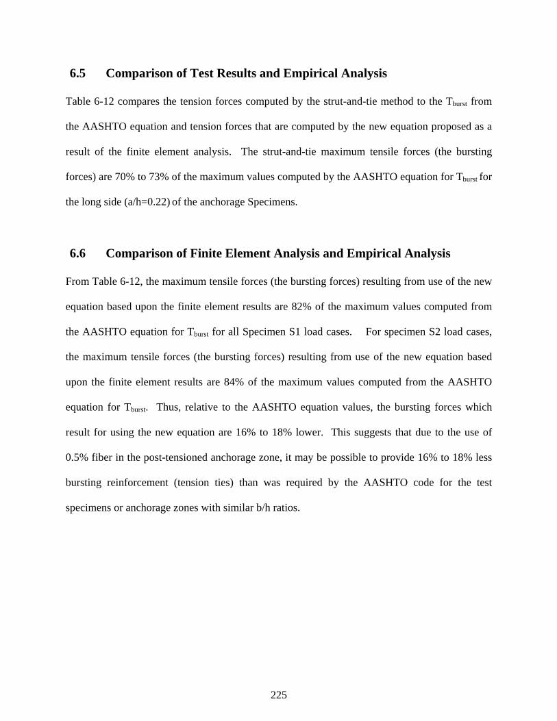
225
6.5 Comparison of Test Results and Empirical Analysis
Table 6-12 compares the tension forces computed by the strut-and-tie method to the Tburst from
the AASHTO equation and tension forces that are computed by the new equation proposed as a
result of the finite element analysis. The strut-and-tie maximum tensile forces (the bursting
forces) are 70% to 73% of the maximum values computed by the AASHTO equation for Tburst for
the long side (a/h=0.22) of the anchorage Specimens.
6.6 Comparison of Finite Element Analysis and Empirical Analysis
From Table 6-12, the maximum tensile forces (the bursting forces) resulting from use of the new
equation based upon the finite element results are 82% of the maximum values computed from
the AASHTO equation for Tburst for all Specimen S1 load cases. For specimen S2 load cases,
the maximum tensile forces (the bursting forces) resulting from use of the new equation based
upon the finite element results are 84% of the maximum values computed from the AASHTO
equation for Tburst. Thus, relative to the AASHTO equation values, the bursting forces which
result for using the new equation are 16% to 18% lower. This suggests that due to the use of
0.5% fiber in the post-tensioned anchorage zone, it may be possible to provide 16% to 18% less
bursting reinforcement (tension ties) than was required by the AASHTO code for the test
specimens or anchorage zones with similar b/h ratios.
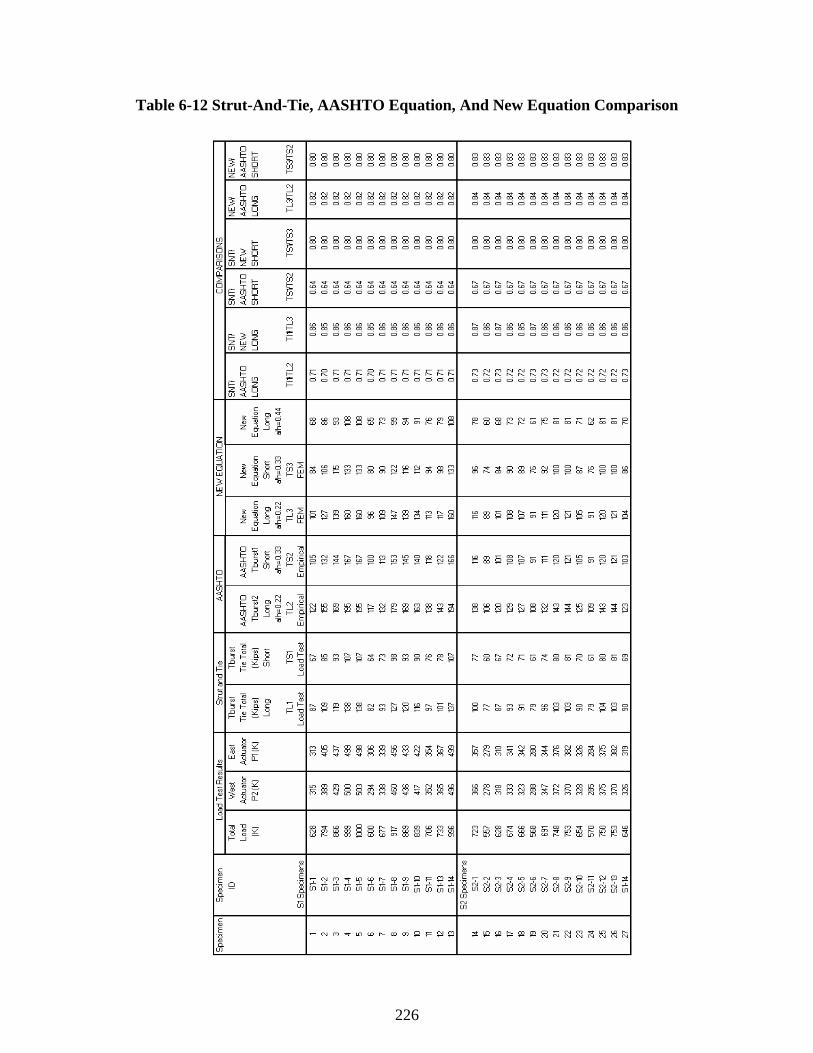
226
Table 6-12 Strut-And-Tie, AASHTO Equation, And New Equation Comparison

227
6.7 Cost Comparison for Reinforced Concrete and Fiber Reinforced
Concrete
In an effort to estimate whether the addition of steel fibers to post-tensioned anchorage zones of
bridge segment will result in a significant cost change, the authors solicited information from the
Florida Department of Transportation’s Construction Estimates Section and several prestressed
concrete manufacturers. In addition, the authors used material cost data and construction
drawings from two bridge projects completed in Florida to consider cost effects. The results of
these cost considerations are discussed in this chapter.
Only one concrete products manufacturer provided information as requested. Pomeroy
Corporation supplied the cost information by considering the Manteca Box Girder project. This
project consisted of 20-3’ W xs3’7” H x 100’ L box girders. Each box segment was
approximately 24 CY of concrete. The following cost data is based upon using Novomesh 850
at a cost of $0.74 per lb and a dosage rate of 66 lb of per CY of concrete (0.5% fiber by volume):
if the amount of black rebar is reduced by 50%, the cost of steel is reduced by 15% relative to the
total materials costs. The concrete cost increases by 55% and is a 12.41% increase relative to
total material costs. The labor cost is reduced by 12 to 20%. The total cost of materials
decreases by 5.9%. The retail price decreases by 8%. These cost changes were dependent upon
material costs prevailing in Summer 2007.
A representative of Unistress Corporation did not have any cost data to share but did speculate
that adding fibers would result in an increase in costs due to the alteration in batching procedure.
One steel fiber manufacturer did not readily supply material costs. A representative of another
228
fiber retailer suggested that adding steel fibers at the dosage rate 66 lb per cubic yard (0.5% fiber
by volume) could result in a material costs increase of approximately $75.00 per cubic yard of
concrete. A sales representative for Novomesh 850, stated that a 24 lb bag of the steel and
polypropylene fiber blend costs approximately $20.00/ bag. So for 66 lbs per cubic yard, the
cost of fibers would be approximately $60.00 plus tax. A representative of The Florida
Department of Transportation’s Estimating Section did supply cost data from a recent
construction project, State Road No. 9 (I-95)/ SR9A (I-295) North Interchange. This project is
located in Jacksonville, Florida.
Using the information obtained, the authors concluded that the addition of steel fibers to concrete
and a 40% reduction of non-prestressed steel in the post-tensioned anchorage zone of bridge
segment will not result in a significant change in the costs of bridge segments for a precast
segmental superstructure. Based upon the calculations and cost considerations used only a
0.44% cost savings would result. However, a 40% reduction in non-prestressed reinforcement
may not be feasible with other design requirements. For a reduction in steel of 36% or less, the
use of fibers would result in an increase in material and labor costs based upon the cost
assumptions made. The information considered to reach this conclusion is summarized in Table
6-13.

229
Table 6-13: Construction Cost Estimates For Precast Segmental Superstructure Table 10.1: Construction Cost Estimates For Precast Segmental Superstructure
With and Without Steel Fiber ReinforcementSample Bridge Project: SR 9/SR9A Let in April 2007
Item # Item Units Quantity Average Unit Price Extended PriceWithout Steel Fibers:
1 Concrete: Class V, Precast Segmental Superstructure CY 7830.2 $1,324.50 $10,371,099.902 Steel: Reinforcing Steel-Superstructure LB 1367927 $0.85 $1,162,737.953 Reinforcing Steel Labor Costs LB 1367927 $0.32 $437,736.64
Cost $11,971,574.49
With Steel Fibers & 40% Less Reinforcing Steel :1 Concrete: Class V, Precast Segmental Superstructure CY 7830.2 $1,324.50 $10,371,099.902 Steel: Reinforcing Steel-Superstructure LB 820756.2 $0.85 $697,642.773 Reinforcing Steel Labor Costs LB 820756.2 $0.32 $262,641.984 Steel Fibers CY 7830.2 $75.00 $587,265.00
Cost $11,918,649.65Cost Decrease $52,924.84
% Savings 0.44%
With Steel Fibers & 36% Less Reinforcing Steel :1 Concrete: Class V, Precast Segmental Superstructure CY 7830.2 $1,324.50 $10,371,099.902 Steel: Reinforcing Steel-Superstructure LB 875473.28 $0.85 $744,152.293 Reinforcing Steel Labor Costs LB 875473.28 $0.32 $280,151.454 Steel Fibers CY 7830.2 $75.00 $587,265.00
Cost $11,982,668.64Cost Increase -$11,094.15
% Increase -0.09%
Considering a 50% reduction in steel and the addition of 66 lb/CY of Novomesh fiber, Pomeroy
Corporation estimated an 8% reduction in retail costs. Based upon a 40% reduction in steel, the
author has estimated less than a 1% reduction in cost. Thus, it is possible that steel fibers can be
added to post-tensioning anchorage zones without altering the costs of construction significantly.
However, in addition to considering material and labor direct costs, a potential cost savings may
be associated with time saving associated with installing less steel reinforcement. For instance,
if the labor productivity rate for installing rebar (size no. 6 and larger) is 800-1000 lbs of steel
per 8 hour day, then installing 40% less steel would save approximately 4377 to 5471 man hours.

230
6.7.1 Cost Comparison for Reinforced Concrete and Fiber Reinforced Concrete
As stated above it is possible to presume that reducing the amount of steel congestion in post-
tensioning anchorage zone may have beneficial effects related to construction costs. When less
steel exists in the post-tensioning anchorage zone, the potential is reduced for construction delays
related to steel congestion. This could lead to significant dollar savings by the avoidance of
construction delays and associated construction claims. Figure 6-19 and Figure 6-20 show
examples of steel congestion in bridge segments.
Figure 6-19: Steel Congestion in Post-Tensioning Anchorage Zone
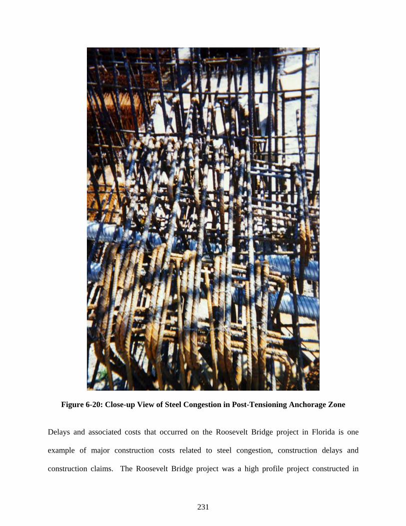
231
Figure 6-20: Close-up View of Steel Congestion in Post-Tensioning Anchorage Zone
Delays and associated costs that occurred on the Roosevelt Bridge project in Florida is one
example of major construction costs related to steel congestion, construction delays and
construction claims. The Roosevelt Bridge project was a high profile project constructed in

232
Stuart, Florida in the mid-1990. The project included the integral pier being cast integrally with
box girder pier segments. Post-tensioned anchorage zones existed in the pier segments. Figure 6-
21 shows a constructed pier segment. In Figure 6-22 a close-up picture of the top of pier rebar
shows rebar spacing problems which occurred due to fabrication and construction tolerances.
Figure 6-21: Pier Segment of the Roosevelt Bridge

233
Figure 6-22: Roosevelt Bridge Pier Segment Reinforcing Steel with Fabrication Issues
Due to the design of the pier segment reinforcement and related construction tolerances, the
contractor was unable to properly construct the integral pier. The vertical steel in the pier
segment was difficult to fit into the forms and conflicted with the location of the longitudinal
post-tensioning ducts in the bottom flange of the box girder. A section drawing of the fixed pier
which shows the longitudinal ducts in the bottom flange is shown in Figure 6-23.
Figure 6-23: Cross-Section of Roosevelt Bridge Pier Segment
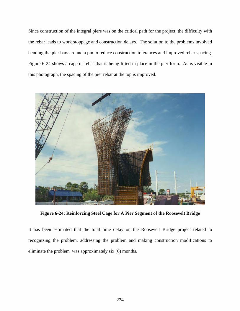
234
Since construction of the integral piers was on the critical path for the project, the difficulty with
the rebar leads to work stoppage and construction delays. The solution to the problems involved
bending the pier bars around a pin to reduce construction tolerances and improved rebar spacing.
Figure 6-24 shows a cage of rebar that is being lifted in place in the pier form. As is visible in
this photograph, the spacing of the pier rebar at the top is improved.
Figure 6-24: Reinforcing Steel Cage for A Pier Segment of the Roosevelt Bridge
It has been estimated that the total time delay on the Roosevelt Bridge project related to
recognizing the problem, addressing the problem and making construction modifications to
eliminate the problem was approximately six (6) months.

235
In the final analysis, the cost associated with the penalty for delay (approximately $20,000/day)
and the payment for accelerating the project to get back on schedule resulted in a construction
claim being paid to the contractor in the amount of approximately 6 to 7 million dollars. This
was a major cost which was related to steel congestion and fabrication.
Avoiding such high expenditures due to construction problem will be beneficial to the Florida
Department of Transportation. Thus, if the use of steel fiber reinforced concrete (SFRC) in the
post-tensioned anchorage zones can reduce steel congestion in these zones, using SFRC may be
very beneficial to the FDOT.
Source: Interview of Tom Andres, FDOT Structures Engineer, on March 28, 2008, Tallahassee,
Florida.

236
CHAPTER 7
CONCLUSIONS AND RECOMMENDATIONS
7.1 Conclusions
An examination of the material test data and the finite element analysis revealed that using
greater than 0.5% fiber by volume does not assure an increase in the average compressive
strength of the concrete. For both Dramix and Novomesh fibers, the concrete with 1.0% fiber
had lower average compressive strengths than the concrete with 0.5% fibers and the concrete
with 0.75% fibers had approximately the same compressive strength as the concrete with 0.5%
fibers. Just as was the case for the compressive strengths tests, the split tensile strength test
results showed that using fiber percentages greater than 0.5% by volume did not guarantee
higher tensile strengths. These results were based upon material tests on 6”x12” concrete
cylinders.
Based upon the seven (7) batches cast with Helix, the following observations were made:
o If the concrete slump was very small, the compressive strength was low. As the Helix
fiber percentage increased, there was a greater tendency for steel balls to develop in the
mix.
o The formation of steel balls probably contributed to low compressive strengths.

237
Based upon the six (6) batches cast with Dramix fibers, the following observations were made:
o Using 0.75% and 1.0% fiber did not greatly improve the concrete compressive strength
above similar mixes with much less fiber.
o While relatively high compressive strength and adequate slumps were achieved with
1.0% Dramix fiber, using fiber percentages greater than 0.5% was not necessary.
o Comparing concrete with Dramix fiber to the same concrete mix with Helix fiber showed
that greater concrete slumps and compressive strengths were achieved for the concrete
with Dramix fibers.
Based upon the seven (7) batches cast with Novomesh fibers, the following observations were
made:
o Even with the variations in the concrete mixes, the compressive strength of the concrete
containing Novomesh fibers had much less fluctuation than the Helix mixes and slightly
less fluctuation that the Dramix mixes.
o Even with the variations in the concrete mixes, the compressive strength of the concrete
containing Novomesh fibers was within 2% or greater than the design strength of 4000
psi.
o Using 0.75% and 1.0% fiber did not necessarily improve the concrete compressive
strength above similar mixes with much less fiber.
o Given the variation in compressive strength, using more than 0.5% fiber may not be
beneficial.
238
o Comparing concrete with Novomesh fiber to the same concrete mix with Helix fiber
showed that greater compressive strengths were achieved for the concrete with
Novomesh fibers.
o Comparing concrete with Novomesh fiber to the same concrete mix with Dramix fiber
showed that greater concrete slumps and compressive strengths were achieved for the
concrete with Dramix fibers.
Based upon all of the material tests, the following observations were made:
o For all batches of concrete (Batches 1 to 35) tested, the measured split tensile strengths
for fiber reinforced concrete were less than the tensile strength computed from the
AASHTO equation:
f’t = 0.23 √f’c 7.1
o For all cases except for cylinders with Helix fibers, the measured modulus was less than
the AASHTO computed value. The modulus of elasticity for the Helix fiber reinforced
concrete was 2% greater than the value computed using the AASHTO equation.
o According to the AASHTO LRFD Bridge Design Specifications (2007), the Poisson’s
ratio can be assumed to be 0.2 if physical tests are not conducted.
o The measured values for Poisson’s ratio were 0.21, 0.22, 0.23 and 0.25 for plain concrete,
Dramix fiber concrete, Helix fiber concrete and Novomesh fiber concrete, respectively
o For Batch 1 to 4, for all of the Helix cylinders except for the cylinders with 0.75% fiber,
the modulus of rupture was greater than the AASHTO range. For the H0.36 cylinders
239
(0.36% fiber) the modulus of rupture was 919 psi which was 17% greater than the
AASHTO value.
o For Anchorage Test Specimens S2 which had Dramix fibers (Specimens S2-2 to S2-5),
the modulus of rupture was greater than the AASHTO range.
o For the Helix and Novomesh cylinders from the S2 Specimens, the modulus of rupture
values was within the AASHTO range.
o There was less than a 10% difference in high and low modulus of rupture test values for
three different fibers.
o Given the variation in compressive strength, using more than 0.5% fiber may not be
beneficial.
Based upon all of the finite element analysis results, the following observation were made:
o The finite element analysis showed that using higher amounts of fiber reinforcement
(0.75% and 1.0%) did not improve the anchorage zone performance much above the
performance that could be achieved by using 0.5% fibers.
o Based upon the nine (9) different finite element (FE) models considered in this research
for a box girder bridge segment, Johnson (2006) concluded that adding steel fibers at a
percentage of 0.5% would be beneficial for the post-tensioning anchorage zone.
o The finite element analysis showed that using higher levels of fiber reinforcement (0.75%
and 1.0%) did not improve the anchorage zone performance much above the performance
that could be achieved by using 0.5% fibers.
Consideration of both S1 and S2 Specimens test results showed the following:

240
o Adding 0.5% steel fibers to the concrete mix without adding non-prestressed
reinforcement in the local and general anchorage zones resulted in test specimens having
load capacities that ranged from 77% to 134% of the load capacity of test specimens with
plain concrete, 100% of the local zone reinforcement recommended by the anchorage
manufacturer and 100% of the general zone reinforcement recommended by the
approximate design method of the AASHTO code.
o Adding steel spiral along with the 0.5% steel fibers resulted in strength increases of up to
22%. However, for two specimens cast with Novomesh fibers (S1-11 and S2-11) the
addition of spiral did not result in increase in strength instead a 13% to 17% decrease in
strength resulted.
o Adding steel ties along with the 0.5% steel fibers resulted in strength increases of up to
32%.
o Even though the addition of 0.5% steel fibers did add up to 37% increase in strength to
test specimens, steel spirals and steel ties are needed to prevent sudden failure
due to punching shear at the anchors (in the local zone) and to prevent sudden failure due
to bursting tension in the general zones.
o With 0.5% fibers by volume, 50% of steel spirals (recommended by PT anchor
manufacturers) and 40% of steel ties (based upon AASHTO design guidelines) , the load
capacities of the anchorage zone test specimens were from 92% to 159% the load
capacity of the plain specimens with the recommend local and general zone
reinforcement. Thus, the addition of steel fibers did increase the strength of the anchorage
zone even with significant reductions in non-prestressed reinforcing steel.

241
o In addition, to improving the strength of the specimens, the addition of fibers (steel and
steel with polypropylene fibers) resulted in smaller and few cracks developing of the
surface of the test specimens. Thus, the use of fibers in PT anchorage zones may
contribute to improvements in the durability of structural elements.
Based upon the maximum loads in the anchorage load tests, the strut-and-tie maximum tensile
forces (the bursting forces) computed are 70% to 73% of the maximum values computed by the
AASHTO equation for Tburst.
The following equation is proposed for computing the tensile bursting force in post-tensioning
anchorage zones when steel fibers are used in the concrete. This equation considers both the
percentage of steel fibers by volume and b/h ratio:
Tma x= 0.23 P [ 1- 1.11(b/h) - 0.15 (F%) + 0.15 (b/h) (F%)] 7.2
Where P = the maximum factored tendon force, h= the transverse dimension of the anchor zone,
b= the width of the anchorage plate, and F%= the percentage of steel fiber by volume.
The strut-and-tie maximum tensile forces (the bursting forces) computed are 85% to 87% of the
maximum values computed by the new equation proposed based upon the finite element results.
Comparison of the bursting force values resulting from the new equation to the bursting tensile
forces (Tburst) resulting from the AASHTO equation, shows that new equation values are 16% to
242
18% less than the AASHTO values. Thus, the experimental results suggest that the results
computed the equation may be quite reasonable.
The maximum tensile forces (the bursting forces) resulting from use of the new equation based
upon the finite element results are 82% of the maximum values computed from the AASHTO
equation for Tburst for all Specimen S1 load cases.
For Specimen S2 load cases, the maximum tensile forces (the bursting forces) resulting from use
of the new equation based upon the finite element results are 84% of the maximum values
computed from the AASHTO equation for Tburst. Thus, relative to the AASHTO equation
values, the bursting forces which result for using the new equation are 16% to 18% lower. This
suggest that due to the use of 0.5% fiber in the test in the post-tensioned anchorage zone, it may
be possible to provide 16% to 18% less bursting reinforcement (tension ties) than are required by
the AASHTO code. According to the finite element analysis on the anchorage test specimens
and the proposed equations, using higher percentages of steel fiber will lead to higher reductions
in the bursting force. The percentage of reduction in the bursting force is related to the b/h ratio
and the percentage of fibers. According to the proposed equation, with 3.0% fibers and
b/h=0.733, there can be a 77.2% reduction in the tensile bursting force. More load tests are
needed to verify the applicability of the new equation for fiber percentages greater than 0.5%
fiber by volume.
Considering a 50% reduction in steel and the addition of 66 lb/CY of concrete (0.5% fiber by
volume) Pomeroy Corporation estimated an 8% reduction in retail costs. Based upon a 40%

243
reduction in steel, the author has estimated less than a 1% reduction in cost. Thus, it is possible
that steel fibers can be added to post-tensioning anchorage zones without altering the costs of
construction significantly.
Comparison of experimental and analytical results showed that steel fibers can be added to
concrete to increase the strength of post-tensioned anchorage zones and reduce the bursting and
confinement mild reinforcement required in these zones. Research results suggest that the
addition of steel fibers to concrete post-tensioned anchorage zones may result in labor cost
savings and time savings but may not significantly change the overall project costs.
Based upon load test results, it was found that the addition of 0.5 percent steel fibers by volume
to a post-tensioned concrete anchorage zone with an anchor plate width to transverse section
depth ratio equal to 0.22 and 0.33 could lead to a 40 percent or more reduction in mild steel
reinforcement (steel spiral and ties). The proposed equation was developed based upon finite
element analysis results and takes into consideration the b/h ratio and the percentage of fibers in
the concrete. Depending upon the b/h ratio and the percentage of steel fibers used in the
concrete, the anchorage zone bursting forces computed by the proposed equation may be 15% to
77% less than bursting force values computed by the AASHTO code equation.
7.2 Recommendations
This research suggests that steel fibers can be used successfully to reduce steel congestion in the
anchorage zone without decreasing the capacity of the member. Based upon this research, the
authors recommend that 0.5% steel fiber by volume be used in the concrete. While greater
244
percentages of fiber may produce greater load capacity, this research showed that a greater
percentage of fiber is not required to achieve the desired objective. It is recommend that
confinement reinforcing (spirals) be used in the local zone and bursting steel (steel ties) be used
in the general zone. However, the spacing of this steel can be increased above the current design
recommendations and the current AASHTO recommendations for the approximate design
method. Based upon the load test results for the parameters used in the test specimens, it was
possible to double the tie spacing for the bursting reinforcement.
When designing post-tensioned anchorage zones with steel fibers, it is recommended that the
newly proposed equation be used to take into consideration both the percentage of steel fibers
and the bearing plate to transverse depth ratio. However, to provide greater confirmation that the
proposed equation is applicable for steel fiber percentages greater than 0.5%, it may be necessary
to load test specimens with greater than 0.5% steel fibers by volume. Also, It would also be
beneficial to conduct long term durability tests on concrete specimens with steel fibers to verify
that the strength of steel fiber reinforced concrete members do not become significantly weaker
with time. This study did not include long term durability tests on anchorage test specimens.

245
BIBLIOGRAPHY
ACI Committee 544 (1998). Guide for Specifying, Proportioning, Mixing, Placing and Finishing Steel Fiber Reinforced Concrete, ACI 544.3R-93, American Concrete Institute. ACI Committee 544 (1999). Design Considerations for Fiber Reinforced Concrete, ACI 544.4R-88), American Concrete Institute. ACI Committee 544 (1999). Measurement of Properties of Fiber Reinforced Concrete, ACI 544.2R-89), American Concrete Institute. ACI Committee 544 (2002). State-of-the Art Report on Fiber Reinforced Concrete, ACI 544.1R-96, American Concrete Institute. Ahmed, A., (2001). Characterization of Steel Fiber And/Or Polymer Concrete Mixes and Applications to Slender Rectangular and I-Beams, Ph.D. Dissertation, University of Nevada. Almansa, E. M. and Cavonas, M. F. (1997). “Mix Design of Steel Fiber Reinforced Concrete”, Materiales De Construccion, Vol. 47, No. 247-248, Julio/Septiembre-Octubre/Diciembre. Al-Saadoun, S.S. (1980). A Three-Dimensional Photoelastic Investigation of the Stress Distribution in the Anchorage Zones of Post-tensioned Beams, Master’s Thesis, University of Petroleum & Minerals, Dhahran, Saudi Arabia. American Association of State Highway and Transportation Officials (2007). AASHTO LRFD Bridge Design Specification, Customary U. S. Units, 4th edition, AASHTO: Washington, D.C. American Concrete Institute, Steel Fiber Reinforced Concrete, Compilation 27. American Concrete Institute, Synthetic And Other Non-Metallic Fiber Reinforcement Of Concrete, Compilation 28. ASTM C31/C31M-03a,“Standard Practice for Making and Curing Concrete Test Specimens in the Field”. ASTM C39/C 39M-05,“Standard Test Method for Compressive Strength of Cylindrical Concrete Specimens.” ASTM C78-02,“Standard Test Method for Flexural Strength of Concrete (Using Simple Beam With Third-Point Loading).”

246
ASTM C138/C 138M-01a,“Standard Test Method for Density (Unit Weight), Yield, and Air Content (Gravimetric) of Concrete.” ASTM C143/C 143M-05a,“Standard Test Method for Slump of Hydraulic-Cement Concrete.” ASTM C157/C 157M-04,“Standard Test Method for Length Change of Hardened Hydraulic-Cement Mortar and Concrete”. ASTM C172,“Standard Practice for Sampling Freshly Mixed Concrete.” ASTM C173/C 173M-01,“Standard Test Method for Air Content of Freshly Mixed Concrete by the Volumetric Method”. ASTM C192/C 192M-05,“Standard Practice for Making and Curing Concrete Test Specimens in the Laboratory”. ASTM C293-02,“Standard Test Method for Flexural Strength of Concrete (Using Simple Beam With Center-Point Loading). ASTM C469 -02,“Standard Test Method for Static Modulus of Elasticity and Poisson’s Ratio of Concrete in Compression.” ASTM C512-02,“Standard Test Method for Creep of Concrete in Compression.” ASTM C1550-02,“Standard Test Method for Flexural Toughness of Fiber Reinforced Concrete (Using Centrally Loaded Round Panel)..” Banthia, N., “Toughness Performance of Hybrid (Steel + Polypropylene) Fiber Reinforced Concrete”, Department of Civil Engineering, The University of British Columbia, Vancouver, Canada, V6T1Z4. Barbosa, A. F. and Ribeiro, G. O. (1998). “Analysis of Reinforced Concrete Structures Using Ansys Nonlinear Concrete Model”, Computational Mechanics, Barcelona, Spain. Bayasi, Z., Gebman, M. J., and Hill. H. B., “Steel Fiber Reinforced Concrete Beam-Column Joint Test”, http://kahuna.sdsu.edu/~sfrc/. Bekaert (1998). “Dramix: The Properties of Dramix Steel Fiber Concrete”, Editor, Nemegeer-Harelbeke, D. , N. V. Bekaert S.A. Bernard, E. S. and Pircher, M. (2001). “The Influence of Thickness on Performance of Fiber-Reinforced Concrete in a Round Determinate Panel Test”, Cement, Concrete, and Aggregates, CCAGDP, Vol. 23, No. 1, pp. 27-33.

247
Breen, J.E., Burdet, O., Roberts, C., Sanders, D., and Wollmann, G. (1994). Anchorage Zone Reinforcement for Post-Tensioned Concrete Girders, National Cooperative Highway Research Program Report 356, Washington D.C., pp. 204. Burdet, O.L. (1990). Analysis and Design of Anchorage Zones in Post-Tensioned Concrete Bridges, Ph.D. Dissertation, The University of Texas at Austin. Casanova, P. and Rossi, P. (1997). ”Analysis and Design of Steel Fiber Reinforced Concrete Beams”, ACI Structural Journal, September-October, pp. 595-602. Chaallal, O., Thibodeau, S., Lescelleur, J., and Malenfant, P. (1996). “Steel Fiber or Conventional Reinforcement for Concrete Shearwalls?”, Concrete International, American Concrete Institute, June, pp.39-42. Collins, M. P. and Mitchell, D. (1991). Prestressed Concrete Structures. Englewood Cliffs: Prentice-Hall. Cruso, B.., “Concrete Reinforcement: Nycon Fibers vs. Welded-Wire Fabric”, Nycon/Reinforced Concrete (Form #020199), Nycon, Inc., Westerly, RI Cucchiara, C., Lidia, L. M., Papia, M. (2004) Effectiveness of stirrups and steel fibres as shear reinforcement, Cement and Concrete Composites, Volume 26, Issue 7, pp 777-786. Department of Structural Engineering and Materials, Technical University of Denmark, “Design of Steel Fiber Reinforced Concrete”, RILEM TC 162-TDF: Test and Design Methods for Steel Fiber Reinforced Concrete, Recommendations for Design of Steel Fiber Reinforced Concrete. Dilger, W. H. and Ghali, A. (1974). “Remedial Measures For Cracked Webs of Prestressed Concrete Bridges”, Journal – Prestressed Concrete Institute, Vol. 19, No. 4, July/August, pp 76-85. Dwarakanath, H.V. and Nagaraj, T.S. (1991). “Comparative Study of Predictions of Flexural Strength of Steel Fiber Concrete”, ACI Structural Journal, November-December, pp. 714-719. Dwarakanath, H.V. and Nagaraj, T.S. (1992). “Deformational Behavior of Reinforced Fiber Reinforced Concrete Beams in Bending”, Journal of Structural Engineering, Volume 118, No. 10, November. Florida Department of Transportation (1989). Post-Tensioning Manual: A Guide to Post-Tensioning of Bridges, Tallahassee: Florida Department of Transportation. Franzen, T. (1992). “Shotcrete For Underground Support: A State-of–the-Art Report With Focus on Steel-Fiber Reinforcement”, Tunneling and Underground Space Technology, Volume 7, Number 4, pp. 383-390.
248
Gaylord, Jr., E. H. and Charles G. N. (editors) (1990). Structural Engineering Handbook, 3 rd. Edition. New York: McGraw-Hill Publishing Company. Gebman, M. (2001). Application of Steel Fiber Reinforced Concrete in Seismic Beam-Column Joints, Master’s Thesis, San Diego State University. Guerrini, G. L., Rosati, G., and Ragazzi, L., “Flexural Behavior of Prestressed Fiber Reinforced Concrete Bridge Beams”. Harajli, M. H., and Salloukh, K. A. (1997). Effect of Fibers on development/ Splice Strength of Reinforcing Bars in Tension, ACI Materials Journal, July-August, pp. 317-324. Haroon, S. A. (2003). Application of Fiber Reinforced Concrete in the End Zones of Precast Prestressed Bridge Girders, Ph.D. Dissertation, Florida State University, FAMU-FSU College of Engineering. Hengprathanee, S. (2004). Linear and Nonlinear Finite Element Analyses of Anchorage Zones in Post-Tensioned Concrete Structures, PH.D. Dissertation, Virginia Polytechnic Institute and State University. Hsu, L. S. and Hsu, C.T. (1994). “Stress-Strain Behavior of Steel-Fiber High Strength Concrete Under Compression”, ACI Structural Journal, July-August, pp. 448-457. Hsu, C.T., He., R. L., and Ezeldin, A. S. (1992). “Load Deformation Behavior of Steel Fiber Reinforced Concrete Beams”, ACI Structural Journal, November-December, pp. 650-657. Huang, Ti (1959). An Experimental Study of Stresses In The End Blocks Of Post-Tensioned Prestressed Concrete Beams, Ph. D. Dissertation, The University of Michigan. Jo, B., Byun, Y., and Tae, G. (2002). “Structural Behavior of Cable Anchorage Zones in Prestressed Concrete Cable-Stayed Bridge”, Canadian Journal of Civil Engineering, 29:171-180. Johnson, S. (2006). Analytical Modeling of Fiber Reinforced Post-Tensioned Concrete Anchorage Zones, Master’s Thesis, Florida State University. Junior, S. F. and Hanai, J. B. (1999). ”Prestressed Fiber Reinforced Concrete Beams with Reduced Ratios of Shear Reinforcement”, Cement & Concrete Composites, Vol. 21, No. 3, pp. 213-217. Khajuria, A., Bohra, K. and Balaguru, P., “Long-Tern Durability of Synthetic Fibers in Concrete”, SP 126-46, American Concrete Institute. Libby, J. R. (1990). Modern Prestressed Concrete: Design Principles and Construction Methods, 4th edition. New York: Van Nostrand Reinhold.

249
Lin, T. Y. and Ned H. Burns (1981). Design of Prestressed Concrete Structures, 3 rd. Edition, New York: John Wiley & Sons. Moens, J. and Nemegeer, D. (1991). ”Designing Fiber Reinforced Concrete Based on Toughness Characteristics”, Concrete International, November, pp. 38-42. Natarajaa, M.C., Nagarajb, T.S., and Basavaraja, S. B (2005) Reproportioning of steel fiber reinforced concrete mixes and their impact resistance, Cem. Concr. Res. (35): 2350-2359. Nawy, Edward G. (1996). Prestressed Concrete: A Fundamental Approach, 2nd ed. Upper Saddle River: Prentice-Hall. Naaman, A. (1998). “New Fiber Technology”, Concrete International, July, pp. 57-62. Narayanan, R. and Darwish, I.Y.S. (1987). “Use of Steel Fibers As Shear Reinforcement”, ACI Structural Journal, May-June, pp. 216-227. Orabone, Bill (2007). Polytorx, e-mail from [email protected] to Brenda Robinson. Pacios, A. and Canovas, M. F. (1997). “Interface Study of Reinforced Concrete”, Materiales De Construccion, Vol 47, no. 247-248, Julio/Septiembre-Octubre/Diciembre. Podony, Jr., W. and Muller, Jean M. (1982). Construction and Design of Prestressed Concrete Segmental Bridges, John Wiley & Sons: New York. Polytorx, Helix Product Profile, pp1-2. Post-Tensioning Institute (1972). Post-Tensioning Manual, 4th edition, Phoenix: Post-Tensioning Institute. Post-Tensioning Institute (1978). Post-Tensioned Box Girder Bridge Manual, Phoenix: Post-Tensioning Institute. Post-Tensioning Institute (1978). Precast Segmental Box Girder Bridge Manual, Phoenix: Post-Tensioning Institute. Ramakrishnan, V., Wu, G.Y., and Hosalli, G., “Flexural Behavior and Toughness of Fiber Reinforced Concretes”, Transportation Research Record 1226, pp. 69-77. Roberts, C. (1990). Behavior And Design Of The Local Anchorage Zone Of Post-Tensioned Concrete, M.S. Thesis, The University of Texas at Austin. Roberts-Wollmann, C.L. (1994). Load Transfer Test with Anchorage CS 5-31, North Carolina University Structures Lab, September.

250
Roberts-Wollmann, C.L. and Breen, John E. (2000). “Design and Test Specifications for Local Tendon Anchorage Zones”, ACI Structural Journal, November-December, pp. 867-875. Sanders, D.H. (1990). Design and Behavior of Post-Tensioned Concrete Anchorage Zones, Ph.D. Dissertation, The University of Texas at Austin. Sanguineti, Dante (2007). E-mail From Dante.Sanguineti@wgint to Brenda Robinson. Shaaban, A. M. and Gesund, H. (1993). “Splitting Tensile Strength of Steel Fiber Reinforced Concrete Cylinders Consolidated by Rodding or Vibration”, ACI Materials Journal, July/August 1993, pp. 356-369. Shah, S. P., Sarigaphuti, M. and Karaguler, M.E. “Comparison of Shrinkage Cracking Performance of Different Types of Fibers and Wiremesh”, ACI SP 142-1., pp. 1-59. Soroushian, P, Mirza, F., and Alhozaimy, A. (1994). “Bonding of Confined Steel Fiber Reinforced Concrete To Deformed Bars”, ACI Materials Journal, March-April, pp. 141-149. Soroushian, P. and Bayasi, Z. (1987). “Prediction of Tensile Strength of Steel Fiber Reinforced Concrete: A Critique of the Composite Material Concept”, American Concrete Institute, SP-105-4., pp. 71-84. Soroushian, P. and Lee, C. (1990). “Tensile Strength of Steel Fiber Reinforced Concrete: Correlation with Some Measures of Fiber Spacing”, ACI Materials Journal, November-December, pp. 541-546. Swamy, R. N. and Al-Ta’an, Sa’ad A. (1981). “Deformation And Ultimate Strength In Flexure Of Reinforced Concrete Beams Made With Steel Fiber Concrete”, ACI Journal, September-October, pp. 395-405. Tan, K. H., Paramasivam, P., and Tan, K.C. (1994). ”Instantaneous and Long-Term Deflections of Steel Fiber Reinforced Concrete Beams”, ACI Structural Journal, July/August, pp. 384-393. Vondran, G. L. (1991). “Application of Steel Fiber Reinforced Concrete”, Concrete International, November, pp. 44-49. VSL Corporation (1996). VSL Post-Tensioning Systems, Litho, Singapore. VSL Corporation (2002). “VSL Post-Tensioning Systems”, Website of VSL Structural Group. VSL International LTD. Detailing For Post-Tensioning, 3 VSL Report Series, Bern, Switzerland. Wafa, F. F., Hasnat, A. and Tarabolsi, O. F. (1992). “Prestressed Fiber Reinforced Concrete Beams Subjected to Torsion”, ACI Structural Journal, May-June, 272-283.

251
Winter, G. and Nilson, A. H. (1979). Design of Concrete Structures, McGraw-Hill: New York, Ninth Edition. Wollman, G.P. (1992). Anchorage Zones in Post-Tensioned Concrete Structures, Ph.D. Dissertation, The University of Texas at Austin. Wollmann, G.P., and Roberts-Wollmann, C.L. (2000). “Anchorage Zone Design”, Preprint of Chapter VIII, Post-Tensioning Manual, Sixth Edition, pp. 46. Wollmann, G.P., and Roberts-Wollmann, C.L. (2000). Anchorage Zone Design, Post-Tensioning Institute. Yazdani, N., Spainhour, L., and Haroon, S. (2002). Application of Fiber Reinforced Concrete in the End Zones of Precast Prestressed Bridge Girders, Florida Department of Transportation Report. Yazdani, N., Tawfiq, K. (2004). “Post-Tensioned Bridge Girder Anchorage Zones Enhancement With Fiber Reinforced Concrete (FRC)”, Proposal Submitted to the Florida Department of Transportation. FAMU-FSU College of Engineering, September. Zellers, B., “Steel and Synthetic Fiber Blends”, Steel/Synthetic Fiber Blends (Form #120102), Nycon, Inc., Westerly, RI. Zellers, Robert (2004). “High Cost of Steel Not the Only Reason for Using Fibers as Shotcrete Reinforcement”, Shotcrete, Fall , pp. 2-4.