post-main-sequence planetarysystemevolution

rsos.royalsocietypublishing.org

ReviewCite this article: Veras D. 2016Post-main-sequence planetary systemevolution. R. Soc. open sci. 3: 150571.http://dx.doi.org/10.1098/rsos.150571

Received: 23 October 2015Accepted: 20 January 2016

Subject Category:Astronomy

Subject Areas:extrasolar planets/astrophysics/solar system

Keywords:dynamics, white dwarfs, giant branch stars,pulsars, asteroids, formation

Author for correspondence:Dimitri Verase-mail: [email protected]

Post-main-sequenceplanetary system evolutionDimitri VerasDepartment of Physics, University of Warwick, Coventry CV4 7AL, UK

The fates of planetary systems provide unassailable insightsinto their formation and represent rich cross-disciplinarydynamical laboratories. Mounting observations of post-main-sequence planetary systems necessitate a complementary levelof theoretical scrutiny. Here, I review the diverse dynamicalprocesses which affect planets, asteroids, comets and pebblesas their parent stars evolve into giant branch, white dwarfand neutron stars. This reference provides a foundation for theinterpretation and modelling of currently known systems andupcoming discoveries.

1. IntroductionDecades of unsuccessful attempts to find planets around otherSun-like stars preceded the unexpected 1992 discovery ofplanetary bodies orbiting a pulsar [1,2]. The three planets aroundthe millisecond pulsar PSR B1257+12 were the first confidentlyreported extrasolar planets to withstand enduring scrutiny due totheir well-constrained masses and orbits. However, a retrospectivehistorical analysis reveals even more surprises. We now know thatthe eponymous celestial body that Adriaan van Maanen observedin the late 1910s [3,4] is an isolated white dwarf (WD) with ametal-enriched atmosphere: direct evidence for the accretion ofplanetary remnants.

These pioneering discoveries of planetary material aroundor in post-main-sequence (post-MS) stars, although exciting,represented a poor harbinger for how the field of exoplanetaryscience has since matured. The first viable hints of exoplanetsfound around MS stars (γ Cephei Ab and HD 114762 b) [5,6],in 1987–1989, were not promulgated as such due to uncertaintiesin the interpretation of the observations and the inability toplace upper bounds on the companion masses. A confidentdetection of an MS exoplanet emerged with the 1995 discoveryof 51 Pegasi b [7], followed quickly by 70 Virginis b [8] and 47Ursae Majoris b [9], although in all cases the mass degeneracyremained. These planets ushered in a burgeoning and flourishingera of astrophysics. Now, two decades later, our planet inventorynumbers in the thousands; over 90% of all known exoplanetsorbit MS stars that will eventually become WDs, and WDs willeventually become the most common stars in the Milky Way.

2016 The Authors. Published by the Royal Society under the terms of the Creative CommonsAttribution License http://creativecommons.org/licenses/by/4.0/, which permits unrestricteduse, provided the original author and source are credited.

http://crossmark.crossref.org/dialog/?doi=10.1098/rsos.150571&domain=pdf&date_stamp=

mailto:[email protected]

2

rsos.royalsocietypublishing.orgR.Soc.opensci.3:150571

................................................abbreviations:

section 1: Introduction section 2: Stellar evolution key points

2.1: Single star evolution 2.2: Common envelope and binary star evolution

section 3: Observational motivation 3.1: Planetary remnants in and around WDs3.2: Major and minor planets around WDs3.3: Subgiant and giant star planet systems3.4: Putative planets in post-CE binaries

AGB: asymptotic giant branchCE: common envelopeGB: giant branchMS: main sequence NS: neutron star RGB: red giant branchSB: substellar bodySN: supernovaWD: white dwarf

3.5: Pulsar planets3.6: Circumpulsar asteroid and disc signatures

section 4: Stellar mass ejecta4.1: The mass-variable point-mass two-body problem4.2: The mass-variable solid body two-body problem4.3: Stellar wind/gas/atmospheric drag

section 5: Star–planet tides5.1: Tidal theory

often-used variables:

5.2: Simulation resultssection 6: Stellar radiation

6.1: Giant branch radiation6.2: Compact object radiation

section 7: Multi-body interactions7.1: Collisions within debris discs

a semimajor axise eccentricityG gravitational constanti inclinationL luminosity

M massr distanceR radiust timeT temperaturev velocityr density

7.2: One star, one planet and asteroids7.3: One star, multiple planets and no asteroids subscripts:

7.4: Two stars, planets and no asteroids7.5: Two stars, one planet and asteroids7.6: Three stars only

section 8: Formation from stellar fallback

none mutual property of SB and starstar

b binary stellar companiond disc

8.1: Post-CE formation around WDs8.2: Post-SN formation around NSs8.3: Formation from tidal disruption of companions

section 9: WD disc formation from 1st-GEN SBssection 10: WD disc evolutionsection 11: Accretion onto WDssection 12: Other dynamics

section 13: The fate of the solar systemsection 14: Numerical codessection 15: Future directions

12.1: General relativity

15.1: Pressing observations15.2: Theoretical endeavours

12.2: Magnetism12.3: External influences12.4: Climate and habitability

disambiguation equations:2.3: initial-to-final mass relation2.4: WD radius-to-mass relation2.5: WD luminosity-to-mass relation3.2: probability of transit or occultation3.3: duration of transit or occultation4.12: semimajor axis change from SN4.13: escape condition from SN4.14: eccentricity change from SN4.16: accretion rate onto SB4.20: gravitational drag force4.21 + 10.8: frictional drag force5.1: semimajor axis evolution from tides6.1: orbital evolution from stellar radiation9.1: tidal disruption radius

GB

WD

fron

t mat

ter

body

end

mat

ter

NS

Figure 1. Paper outline and nomenclature. Some section titles are abbreviated to save space. Variables not listed here are described insitu, and usually contain descriptive subscripts and/or superscripts. The important abbreviation ‘substellar body’ (SB) can refer to, forexample, a brown dwarf, planet, moon, asteroid, comet or pebble. ‘Disambiguation equations’ refer to relations that have appeared inmultiple different forms in the literature. In this paper, these other forms are referenced in the text that surrounds these equations, so thatreaders can decidewhich form is best to use (or newly derive) for their purposes. Overdots always refer to time derivatives. The expression〈〉 refers to averaged quantities.

Nevertheless, major uncertainties linger. MS exoplanet detection techniques currently provideminimal inferences about the bulk chemical composition of exoplanetary material. How planets form anddynamically settle into their observed states remains unanswered and represents a vigorous area of activeresearch. Calls for a better understanding of post-MS evolution arise from MS discoveries of planets nearthe end of their lives [10] and a desire to inform planet formation models [11]. Direct observation ofMS smaller bodies, such as exo-asteroids, exo-comets or exo-moons, remains tantalizingly out of reach,except in a handful of cases [12–16].

3


................................................

mass ejecta orbital changessection 4

mass ejecta physical changessection 4

star–planet tidessection 5

stellar radiationsection 6

general relativitysection 12a

magnetic fieldssection 12b

galactic tidessection 12c

stellar flybyssection 12c

distance in AU 10–3 10–2

giant branch (GB) phases

10–1 1 10 102 103 104 105

mass ejecta orbital changessection 4

mass ejecta physical changessection 4

star–planet tidessection 5

stellar radiationsection 6

general relativitysection 12a

magnetic fieldssection 12b

galactic tidessection 12c

stellar flybyssection 12c

distance in AU

definitely non-negligible for at least some substellar bodies (SBs)

possibly non-negligible for at least some substellar bodies (SBs)

negligible for all substellar bodies (SBs)

10–3 10–2

white dwarf (WD) and neutron star (NS) phases

10–1 1 10 102 103 104 105

Figure 2. Important forces in post-MS systems. These charts represent just a first point of reference. Every system should be treated ona case-by-case basis. Magnetic fields include those of both the star and the SB, and external effects are less penetrative in the GB phasesbecause they are relatively short.

Post-MS planetary system investigations help alleviate these uncertainties, particularly withescalating observations of exoplanetary remnants in WD systems. Unlike for pulsar systems, planetarysignatures are common in and around WD stars. The exquisite chemical constraints on rockyplanetesimals that are gleaned from WD atmospheric abundance studies is covered in detail by thereview of Jura & Young [17], and is not a focus of this article. Similarly, I do not focus on the revealingobservational aspects of the nearly forty debris discs orbiting WDs, a topic recently reviewed byFarihi [18].

Instead, I place into context and describe the complex and varied dynamical processes that influenceplanetary bodies after the star has turned off of the MS. I attempt to touch upon all theoretical aspects ofpost-MS planetary science, although my focus is on the giant branch (GB) and WD phases of stellarevolution. The vital inclusion of bodies smaller than planets—e.g. exo-asteroids and exo-comets—inthis review highlights both the necessity of incorporating Solar system constraints and models and theinterdisciplinary nature of post-MS planetary science.

4


................................................Table 1. Some notable post-MS planetary systems.

name type sections

BD+48 740a GB star with possible pollution 3.3.1. . . . . . . . . . . . . . . . . . . . . . . . . . . . . . . . . . . . . . . . . . . . . . . . . . . . . . . . . . . . . . . . . . . . . . . . . . . . . . . . . . . . . . . . . . . . . . . . . . . . . . . . . . . . . . . . . . . . . . . . . . . . . . . . . . . . . . . . . . . . . . . . . . . . . . . . . . . . . . . . . . . . . . . . . . . . . . . . . . . . . . . . . . . . . . . . . . . . . . . . . . . . . . . . . . . . . . . . .

G 29-38b WD with disc and pollution 3.1.2. . . . . . . . . . . . . . . . . . . . . . . . . . . . . . . . . . . . . . . . . . . . . . . . . . . . . . . . . . . . . . . . . . . . . . . . . . . . . . . . . . . . . . . . . . . . . . . . . . . . . . . . . . . . . . . . . . . . . . . . . . . . . . . . . . . . . . . . . . . . . . . . . . . . . . . . . . . . . . . . . . . . . . . . . . . . . . . . . . . . . . . . . . . . . . . . . . . . . . . . . . . . . . . . . . . . . . . . .

GD 362c WD with disc and pollution 3.1.2. . . . . . . . . . . . . . . . . . . . . . . . . . . . . . . . . . . . . . . . . . . . . . . . . . . . . . . . . . . . . . . . . . . . . . . . . . . . . . . . . . . . . . . . . . . . . . . . . . . . . . . . . . . . . . . . . . . . . . . . . . . . . . . . . . . . . . . . . . . . . . . . . . . . . . . . . . . . . . . . . . . . . . . . . . . . . . . . . . . . . . . . . . . . . . . . . . . . . . . . . . . . . . . . . . . . . . . . .

GJ 86d binary WD–MS with planet 3.2.2. . . . . . . . . . . . . . . . . . . . . . . . . . . . . . . . . . . . . . . . . . . . . . . . . . . . . . . . . . . . . . . . . . . . . . . . . . . . . . . . . . . . . . . . . . . . . . . . . . . . . . . . . . . . . . . . . . . . . . . . . . . . . . . . . . . . . . . . . . . . . . . . . . . . . . . . . . . . . . . . . . . . . . . . . . . . . . . . . . . . . . . . . . . . . . . . . . . . . . . . . . . . . . . . . . . . . . . . .

NN Sere binary WD–MS with planets 3.4, 7.4.1, 7.4.2, 8.1, 15.1.1. . . . . . . . . . . . . . . . . . . . . . . . . . . . . . . . . . . . . . . . . . . . . . . . . . . . . . . . . . . . . . . . . . . . . . . . . . . . . . . . . . . . . . . . . . . . . . . . . . . . . . . . . . . . . . . . . . . . . . . . . . . . . . . . . . . . . . . . . . . . . . . . . . . . . . . . . . . . . . . . . . . . . . . . . . . . . . . . . . . . . . . . . . . . . . . . . . . . . . . . . . . . . . . . . . . . . . . . .

PSR B1257+12f pulsar with planets 1, 3.5, 7.3.3, 8.2, 8.3. . . . . . . . . . . . . . . . . . . . . . . . . . . . . . . . . . . . . . . . . . . . . . . . . . . . . . . . . . . . . . . . . . . . . . . . . . . . . . . . . . . . . . . . . . . . . . . . . . . . . . . . . . . . . . . . . . . . . . . . . . . . . . . . . . . . . . . . . . . . . . . . . . . . . . . . . . . . . . . . . . . . . . . . . . . . . . . . . . . . . . . . . . . . . . . . . . . . . . . . . . . . . . . . . . . . . . . . .

PSR B1620-26g binary pulsar-WD with planet 3.2.1, 7.4.1. . . . . . . . . . . . . . . . . . . . . . . . . . . . . . . . . . . . . . . . . . . . . . . . . . . . . . . . . . . . . . . . . . . . . . . . . . . . . . . . . . . . . . . . . . . . . . . . . . . . . . . . . . . . . . . . . . . . . . . . . . . . . . . . . . . . . . . . . . . . . . . . . . . . . . . . . . . . . . . . . . . . . . . . . . . . . . . . . . . . . . . . . . . . . . . . . . . . . . . . . . . . . . . . . . . . . . . . .

SDSS J1228+1040h WD with disc and pollution 3.1.2, 10, 15.1.2. . . . . . . . . . . . . . . . . . . . . . . . . . . . . . . . . . . . . . . . . . . . . . . . . . . . . . . . . . . . . . . . . . . . . . . . . . . . . . . . . . . . . . . . . . . . . . . . . . . . . . . . . . . . . . . . . . . . . . . . . . . . . . . . . . . . . . . . . . . . . . . . . . . . . . . . . . . . . . . . . . . . . . . . . . . . . . . . . . . . . . . . . . . . . . . . . . . . . . . . . . . . . . . . . . . . . . . . .

WD 0806-661i WD with planet 3.2.1. . . . . . . . . . . . . . . . . . . . . . . . . . . . . . . . . . . . . . . . . . . . . . . . . . . . . . . . . . . . . . . . . . . . . . . . . . . . . . . . . . . . . . . . . . . . . . . . . . . . . . . . . . . . . . . . . . . . . . . . . . . . . . . . . . . . . . . . . . . . . . . . . . . . . . . . . . . . . . . . . . . . . . . . . . . . . . . . . . . . . . . . . . . . . . . . . . . . . . . . . . . . . . . . . . . . . . . . .

WD 1145+017j WD with asteroids, disc and pollution 3.2.1., 15.1.1. . . . . . . . . . . . . . . . . . . . . . . . . . . . . . . . . . . . . . . . . . . . . . . . . . . . . . . . . . . . . . . . . . . . . . . . . . . . . . . . . . . . . . . . . . . . . . . . . . . . . . . . . . . . . . . . . . . . . . . . . . . . . . . . . . . . . . . . . . . . . . . . . . . . . . . . . . . . . . . . . . . . . . . . . . . . . . . . . . . . . . . . . . . . . . . . . . . . . . . . . . . . . . . . . . . . . . . . .

WD J0959-0200k WD with disc and pollution 3.1.2., 10, 15.1.1. . . . . . . . . . . . . . . . . . . . . . . . . . . . . . . . . . . . . . . . . . . . . . . . . . . . . . . . . . . . . . . . . . . . . . . . . . . . . . . . . . . . . . . . . . . . . . . . . . . . . . . . . . . . . . . . . . . . . . . . . . . . . . . . . . . . . . . . . . . . . . . . . . . . . . . . . . . . . . . . . . . . . . . . . . . . . . . . . . . . . . . . . . . . . . . . . . . . . . . . . . . . . . . . . . . . . . . . .

vMa2l WD with pollution 1, 3.1.1. . . . . . . . . . . . . . . . . . . . . . . . . . . . . . . . . . . . . . . . . . . . . . . . . . . . . . . . . . . . . . . . . . . . . . . . . . . . . . . . . . . . . . . . . . . . . . . . . . . . . . . . . . . . . . . . . . . . . . . . . . . . . . . . . . . . . . . . . . . . . . . . . . . . . . . . . . . . . . . . . . . . . . . . . . . . . . . . . . . . . . . . . . . . . . . . . . . . . . . . . . . . . . . . . . . . . . . . .

aPotentially polluted with lithium.bFirst WD debris disc.cPolluted with 17 different metals.dPlanet orbits the MS star.eMultiple circumbinary planets.f First confirmed exoplanetary system.gFirst confirmed circumbinary planet.hDisc probably eccentric and axisymmetric.iPlanet at several thousand astronomical units.jOnly WD with transiting SBs, a disc and pollution.kHighly variable WD disc.lFirst polluted WD.

1.1. Article layoutI begin by providing a visual table of contents in figure 1, which includes handy references for theabbreviations and commonly used variables in this article. I use the abbreviation ‘SB’ (‘substellar body’or ‘smaller body’) extensively in the text and equations; constraining relations to just one of planets,asteroids, comets or pebbles is too restrictive for the strikingly diverse field of post-MS planetary science.The term also includes brown dwarfs, for which many physical relations presented here also apply.‘Planetary systems’ is defined as systems which include SBs. The ‘disambiguation’ equations identifiedin figure 1 refer to relations that have appeared in multiple different forms in the previous post-MSplanetary literature; I attempt to consolidate these references. In figure 2, I characterize distances fromthe star in which various forces are important, or might be important. This figure may be used as a guidewhen modelling a particular system or set of systems. Table 1 lists some notable post-MS planetarysystems, along with brief descriptions and pointers to where they are mentioned in the text.

My deliberately basic treatment of introductory material (stellar evolution and observations from§§2 to 3) is intended to provide the necessary background for subsequent sections, and not meant toemulate an in-depth synopsis. The body of the article (§§4–12) provides more detail on the dynamicalaspects of post-MS planetary science. This review concludes with brief comments on the fate of the Solarsystem (§13), a hopefully helpful summary of the numerical codes that have or may be used in theoreticalinvestigations (§14) and a promising outlook on the future of this science (§15), with guidance for howupcoming observations can maximize scientific return.

2. Stellar evolution key pointsThe infrangible link between SBs and their host star is highlighted during post-MS evolution, andrequires one to understand the star’s temporal evolution. My treatment below is purposefully simplified

5


................................................to provide the necessary information for post-MS planetary system studies; for more detail, seee.g. [19,20].

2.1. Single star evolution

2.1.1. Main sequence

The MS evolution is important because it provides the historical context and initial conditions fordedicated post-MS studies. MS stars quiescently burn hydrogen to produce helium in their cores, anddo lose mass through winds according to eqn 4 of [21] and eqn 9 of [22]. The Sun currently loses mass ata rate of about 2.4 × 10−14 M� yr−1 (p. 15 of [23]). The MS lifetime is sensitively dependent on the initialvalue of M(MS)

� and less so on the star’s metallicity Z�. This lifetime decreases drastically (by two ordersof magnitude, from about 10 to 0.1 Gyr) as the initial mass increases from 1 to 6 M� (see fig. 5 of [24]).

2.1.2. Giant branches

All stars experience the ‘red giant branch’ (RGB) phase, when hydrogen in the core is exhausted and theremaining hydrogen burns in a contracting shell as the envelope expands. The extent of convection inthe star increases, potentially ‘dredging-up’ already-burnt matter. Eventually, core temperatures becomehigh enough to burn helium. For stars with M(MS)

� < 2.0 M�, helium ignition sets off so-called ‘heliumflashes’. This value of 2.0 M� represents a key transition mass; the duration and character of the massloss changes markedly when crossing this threshold. After the core helium is exhausted, a helium-burning shell is formed. At this point, the star is said to have begun evolving on the ‘asymptotic giantbranch’ (AGB). Another expansion of convection may then cause a ‘second dredge-up’. When, duringthe AGB, the helium-burning shell reaches the hydrogen outer envelope, a different type of helium flashoccurs (denoted a ‘thermal pulse’), one which emits a sudden burst of luminosity and mass. This event,which can occur many times, also causes a sudden increase and then drop in stellar radius (see fig. 3of [25]). Therefore, AGB thermal pulses literally cause the star to pulsate. Changes in the star’s convectiveproperties during this violent time may also allow for a ‘third dredge-up’ to then occur.

During both the RGB and AGB phases, the star undergoes significant mass loss (up to 80%), radiusvariability (up to about 10 AU, from an initial value of 10−3 − 10−2 AU), and luminosity variability (upto many tens of thousand times the MS value) regardless of the extent of the pulses. Figure 3 providesrepresentative values; the highlighted rows indicate the most typical progenitors for the currentlyobserved Milky Way WD population. These changes along the GB phases may completely transforma planetary system; indeed linking WD and MS planetary systems is a goal and a challenge, and mayalso help constrain stellar evolution. Unfortunately, identifying the dominant mechanisms responsiblefor mass loss—both isotropic and anisotropic—on the RGB and AGB continues to prove difficult.

Red giant branch mass loss. On the RGB, mass-loss is traditionally parametrized by the Reimers formula,a series of proportionalities that was later calibrated [28] and recently improved upon [29] to finally give

dM(RGB)�

dt= 8 × 10−14M� yr−1

(L(RGB)

�

L�

)(R(RGB)

�

R�

)(M(RGB)

�

M�

)−1

×(

T(RGB)�

4000 K

)7/2⎡⎣1 + 2.3 × 10−4

(g(RGB)�

g�

)−1⎤⎦ , (2.1)

where g refers to surface gravity. Traditional formulations of equation (2.1), which are still widely used,do not include the final two terms, and have a leading coefficient of 2 × 10−13 M� yr−1.

Asymptotic giant branch mass loss. Applying the Reimers formula on the AGB can produce significantlyerroneous results (fig. 13 of [30]). Instead, during this phase a different prescription is often applied,whose formulation [31] has stood the test of ongoing observations and can be found, for example, ineqns 2–3 of [32]. Accompanying each AGB pulse is a variation in mass loss of potentially a few ordersof magnitude, a phenomenon now claimed to have been observed [33]. At the final stage of the AGB—‘the tip’ of the AGB—the wind is particularly powerful and is known as the ‘superwind’ (e.g. [34]).A star’s peak mass loss rate typically occurs during the superwind unless the AGB phase is non-existentor negligible.

Giant branch mass ejecta speed. The speed at which mass is ejected is generally a function of the internalproperties of the star and the location of ejection. One simplified estimate that may be useful for post-MS

6


................................................MS

stellartype

B3 6.30 1.18 6.19 9.27 × 10–5 2.0 × 10–466200 0.086 0.92

B4 5.00 1.00 4.98 6.51 × 10–5 2.5 × 10–446100 0.25 1.41

B5 4.30 0.91 4.29 5.15 × 10–5 3.0 × 10–435900 0.49 1.89

B8 3.00 0.75 2.86 2.78 × 10–5 4.5 × 10–418700 2.42 4.19

A0 2.34 0.65 2.26 2.33 × 10–5 6.0 × 10–412700 7.71 5.72

A5 2.04 0.64 1.86 1.88 × 10–5 1.4 × 10–39500 20.0 6.27

F0 1.66 0.60 1.55 1.32 × 10–5 0.0407140 88.0 5.24

F5 1.41 0.57 1.35 9.56 × 10–6 0.115800 220 5.08

G0 1.16 0.53 1.15 1.14 × 10–5 0.414520 536 4.82

G2 1.11 0.53 1.11 7.44 × 10–6 0.574300 621 4.77

G5 1.05 0.52 1.07 6.89 × 10–6 0.824130 684 4.77

K0 0.90 0.51 0.92 2.07 × 10–7 4.143590 888 5.01

MSmass

WDmass

(M�) (M�)

maxAGBradius(AU)

maxmass loss

rate(M�/yr)

maxlum-

inosity(L�)

RGBtimespan

(Myr)

AGBtimespan

(Myr)

RGB massloss/

AGB massloss

Figure 3. Useful values for 12 different stellar evolution tracks. I mapped the first column to the second by using appendix B of [26], andthen created the remaining columns by using the SSE code [27] by assuming its default values (which includes Solar metallicity). The fourhighlighted rows roughly represent the range of themost common progenitor stars for the present-dayWD population in theMilkyWay.

studies is [35]

vwind =

√√√√√(2GM�

R�

)⎛⎝1 − [v(rot)� ]

2R�

GM�sin2 θ

⎞⎠, (2.2)

where θ is the stellar co-latitude and v(rot)� is the stellar rotational speed at the equator.

Giant branch changes from substellar body ingestion. If a large SB such as a brown dwarf of planetis ingested during the GB phases, two significant events might result: an enhancement of lithiumin the photosphere and spin-up of the star. The former was predicted in 1967 by Alexander [36].Adamów et al. [37] claimed that SB accretion onto stars can increase their Li surface abundance fora few Myr. However, an enhanced abundance of Li in GB stars could also indicate dredge-up bythe Cameron–Fowler mechanism, mixing through tides, or thermohaline or magneto-thermohalineprocesses. Therefore, a planetary origin interpretation for Li overabundance remains degenerate.

Several investigations have considered how a GB star spins up due to SB accretion. In his eqn 1,Massarotti [38] computed the change in the star’s rotational speed. He suggested that a population ofGB fast-rotators due to planet ingestion would be detectable if the speed increased by at least 2 km s−1.Carlberg et al. [39] found that a few percent of the known population of exoplanets (at the time) couldcreate rapid rotators, where rapid is defined as having a rotational speed larger than about 10 km s−1.

Substellar body ingestion may cause other changes, such as enhanced mass loss [40,41] anddisplacement on the Hertzsprung–Russel diagram [42]. The presence or ingestion of an SB could be areason [43] why some GB stars prematurely lose their entire envelope before core fusion of helium begins.These stars are known as ‘extreme horizontal branch stars’, which are also known as ‘hot subdwarfs’or ‘sdB’ stars (see [44] for a review specifically of these types of stars). This SB ingestion explanationis particularly relevant for hot subdwarfs with no known stellar binary companions. When modelling

7


................................................AGB envelopes for this or other purposes, one may use a power-law density profile (see, e.g. Sec. 2 [45]);Willes & Wu [46] instead gave a more complex form in their eqn 5.

2.1.3. White dwarfs

For stars with M(MS)� � 8 M�, after the GB envelope is completely blown away the remaining core

becomes a WD [27,47,48]. In the Milky Way, about 95% of all stars will become WDs [47]. The term ‘white’in WD originates from the notion that the majority of known WDs are hotter than the Sun [47]. Theexpelled material photoionizes and the resulting observed structure, which might not have any relationto planets whatsoever, is confusingly termed a ‘planetary nebula’. Although the expelled material willencounter remnant planets and asteroids, few investigations so far have tried to link these nebulae withplanets. Even the link between nebula morphology and stellar configurations remains uncertain [49]although SBs that are at least as massive as planets, as well as stellar-mass companions, are thought toplay a significant role in shaping and driving the nebulae (e.g. [50,51]).

The time elapsed since the moment an AGB star becomes a WD is denoted the ‘cooling age’ becausethe WD is in a state of monotonic cooling (as nuclear burning has now stopped). The term cooling ageallows one to distinguish from the total age of the star, which includes its previous evolutionary phases.Although some investigations refer to planetary nebula or ‘post-AGB’ as the name of a separate stellarevolutionary phase [52,53], I do not, and assume that the transition from AGB to WD contains no otherevolutionary phase.

White dwarf designations. WDs have and continue to be characterized observationally by the dominantspectral absorption lines in their atmospheres. These designations [54] include ‘D’, which stands fordegenerate, ‘A’, for hydrogen rich, ‘B’ for helium rich, ‘Z’ for metal-rich (metals are elements heavierthan helium) and ‘H’ for magnetic. About 80–85% of the WD population are DA WDs [47,48]. Non-DAWDs probably lost their hydrogen in a relatively late-occurring shell flash.

White dwarf composition. The composition of the WD core is some combination of carbon (from theburning of helium), oxygen (from the burning of carbon) and rarely neon (from the burning of oxygen).The vast majority of WD cores contain carbon and oxygen because they are not hot enough to hostcopious quantities of oxygen and neon. Only trace amounts of other metals should exist.

White dwarf mass. The initial mass function combined with the current age of the Galaxy has conspiredto yield a present-day distribution of WD masses according to fig. 2 of [47] and figs 8, 10 and 11 of [55].These figures indicate a unimodal distribution that is peaked at about 0.6 M� and contains a longtail at masses higher than 0.8 M�. This distribution also conforms with a previous large (348 objects)survey [56], where 0.4 M� and 0.8 M� values are considered to be ‘low-mass’ and ‘high-mass’ [57].In principle, WD masses can range up to about 1.4 M�. Only single stars with M(MS)

� � 0.8 M� couldhave already become WDs, and hence single WDs must have masses that satisfy M(WD)

� � 0.4 M�. Forcomparable or lower mass single WDs, perhaps substellar companions could have stripped away someof this mass during the CE phase [58].

How the mass of a WD is related to its progenitor MS mass represents an extensive field of studycharacterized by the ‘initial-to-final-mass relation’. Observationally, this relation is often determinedwith WDs that are members of stellar clusters whose ages are well constrained. However, the relationis dependent on stellar metallicity, and in particular the chemistry of individual stars. Ignoring thosedependencies, some relations used in the post-MS planetary literature include eqn 6 of [59] (originallyfrom [60]), eqn 9 of [61] (originally from [21]) and eqn 6 of [62] (originally from [63]).

One study which did evaluate how the initial–final mass relationship is a function of metallicityis Meng et al. [64]. They found that metallicity can change the final mass by 0.4 M�, a potentially alarmingvariation given the difference between a ‘low-mass’ WD (0.4 M�) and a ‘high-mass’ WD (0.8 M�). Menget al. [64] also provided in their appendix potentially useful WD–MS mass relations as a functionof metallicity, for Z� = [0.0001, 0.0003, 0.001, 0.004, 0.01, 0.02, 0.03, 0.04, 0.05, 0.06, 0.08, 0.1]. For Solarmetallicity (Z� = Z� = 0.02) and any star that will become a WD for 0.8 M� < M(MS)

� < 6.0 M�, they found

M(WD)�

M�= min

⎡⎣0.572 − 0.046

M(MS)�

M�+ 0.0288

(M(MS)

�

M�

)2

, 1.153 − 0.242M(MS)

�

M�+ 0.0409

(M(MS)

�

M�

)2⎤⎦ .

(2.3)

White dwarf radius. Usefully for modellers, the radius of the WD can be estimated entirelyin terms of M(WD)

� with explicit formulae. A particularly compact but broad approximation isR(WD)

� /R� ∼ 10−2(M(WD)� /M�)−1/3. Alternatively, more accurate formulae—which are derived assuming

8


................................................that the WD temperature is zero—that are within a few percent of one another are from eqn 15 of [65],and, as shown below, eqns 27–28 of [66]:

R(WD)�

R�≈ 0.0127

(M(WD)

�

M�

)−1/3√√√√1 − 0.607

(M(WD)

�

M�

)4/3

. (2.4)

From equation (2.4), I obtain a canonical WD radius of 8750 km = 0.0126R�, assuming the fiducial valueof M(WD)

� = 0.6 M�.White dwarf luminosity. The luminosity of WDs can be estimated in multiple ways. A rough

approximation that does not include dependencies on stellar mass or metallicity is from eqn 8 of [67],which is originally from Althaus et al. [68]: L� = L(tcool = 0) × [tcool/105 years]−1.25, where tcool is the WDcooling age. I include these dependencies by combining the prescription originally from Mestel [69] withexpressions used in post-MS planetary contexts from eqn 6 of [32] and eqn 5 of [70] to obtain

L(WD)� = 3.26L�

(M(WD)

�

0.6 M�

)(Z�

0.02

)0.4 (0.1 + tcool

Myr

)−1.18, (2.5)

where Z� is the assumed-to-be-fixed stellar metallicity. Depending on the WD cooling age, the star’sluminosity can range from about 103L� to 10−5L�. This formula also applies only until ‘crystallization’sets in, which occurs for T(WD)

� � 6000–8000 K [71].

2.1.4. Neutron stars

For stars with M(MS)� � 8 M�, the end of the AGB phase results in an explosion: a core collapse plus

an outwardly expanding shockwave that nearly instantaneously (with velocities of approx. 103 −104 km s−1) expels the envelope and causes the star to lose at least half of its mass. This event is asupernova (SN). Any asymmetry in the SN will cause a velocity ‘kick’. The remaining stellar corebecomes either a neutron star (NS) or a black hole. Of most relevance to post-MS planetary science arepulsars, which are an august class of NSs that represent precise, stable and reliable clocks.

Although NSs and WDs are together grouped as ‘compact stars’, NSs are much more compact, withradii on the order of 10 km. NS masses are greater than those of WD stars. Typically M(NS)

� ≥ 1.4 M�.NSs cool much faster than WDs, with a decreasing luminosity which can be modelled by (p. 30 of [72])

L(NS)� = 0.02L�

(M(NS)

�

M�

)2/3 [max(tcool, 0.1 Myr)

Myr

], (2.6)

where tcool represents the NS cooling time in this context.Millisecond pulsars have rotational periods on the order of milliseconds. They are thought to have

been spun up by accretion, and are hence said to be ‘recycled’. Miller & Hamilton [73] argued that thepresence of planets around millisecond pulsars can constrain the evolutionary history of the star. Inparticular, they posed that the moon-sized SB around the millisecond pulsar PSR B1257+12 demonstrateshow that particular star is not recycled by (i) favouring a second-generation formation scenario for theSB (see §8) and (ii) suggesting that the formation cannot have occurred during an accretional event norin a post-spin-up disc. They claimed that the moon-sized SB must have formed, post-SN, around the staras is with its current rotational frequency and magnetic moment.

2.2. Common envelope and binary star evolutionStellar binary systems are important because they represent several tens of percent of all Milky Waystellar systems. The presence of a stellar binary companion can significantly complicate the evolution ifthe mutual separation is within a few tens of AU. Both star–star tides and the formation of a ‘commonenvelope’ (CE) can alter the fate otherwise predicted from single-star evolution. Ivanova et al. [74]reviewed the theoretical work performed on and the physical understanding of CEs; see their fig. 1 forsome illustrative evolutionary track examples. Taam & Ricker [75] provided a shorter, simulation-basedreview of the topic.

A CE is a collection of mass that envelopes either (i) two stars or (ii) one star and one large SB likea giant planet. In both cases, as the smaller binary component spirals into the larger one, the formertransfers energy to the envelope. The transfer efficiency is a major unknown in the theory of stellarevolution. The smaller companion may blow off the CE by depositing a sufficient amount of energy in

9


................................................the envelope during inspiral. Relevant equations describing this process include eqn 17 of [76], eqns 2–5 of [77] and eqn 8 of [78]. A more complete treatment that takes into account shock propagation androtation may be found in eqns 6–25 of [77]; also see the earlier work by [79]. The more massive thecompanion, and the more extended the envelope, the more likely ejection will occur. The speed of infallwithin the CE may be expressed generally as a quartic equation in terms of the radial velocity (eqn 9of [51]), but only if the SB’s tangential velocity is known, as well as the accretion rate onto the SB. Eqn 1of [58] approximates the final post-CE separation after inspiral.

Even without a CE, the interaction between both stars might dynamically excite any SBs in thatsystem, particularly when one or both stars leave the MS. Both stars might be similar enough in age(and hence MS mass) to undergo coupled GB mass loss. Section 5.2 of [80] quantified this possibility, andfinds that the MS masses of both components must roughly lie within 10% of one another in order forboth to simultaneously lose mass during their AGB phases.

3. Observational motivationPost-MS planetary systems provide multiple insights that are not available from MS planetary systems,including: (i) substantive access to surface and interior SB chemistry, (ii) a way to link SB fateand formation, (iii) different constraints on tidal, mass-losing and radiative processes and (iv) theenvironments to allow for detections of extreme SBs. The agents for all this insight come from GB, WDand NS planetary systems. Overall, the total number of WD remnant planetary systems is of the sameorder (approx. 1000) as MS planetary systems, and about one order of magnitude more than GB planetarysystems. The number of remnant planetary systems around NSs is a few.

3.1. Planetary remnants in and around white dwarfsFragments and constituents of disrupted SBs that were planets, asteroids, moons, comets, boulders andpebbles observationally manifest themselves in the atmospheres of WDs and the debris discs whichsurround WDs. The mounting evidence for and growing importance of both topics is, respectively,highlighted in recent reviews [17,18]. Here, I devote just one subsection to the observational aspectsof each topic.

3.1.1. White dwarf atmospheric pollution

Because WDs are roughly the size of the Earth but contain approximately the mass of the Sun, WDsare about 105 as dense as the Sun. Consequently, due to gravitational settling, WD atmospheres quicklyseparate light elements from heavy elements [81], causing the latter to sink as oil would in water. Thisstratification of WD atmospheres by atomic weight provides a tabula rasa upon which any ingestedcontaminants conspicuously stand out—as long as we detect them before they sink.

Composition of intrinsic white dwarf photosphere. The chemical composition of the atmosphere isdependent on (i) how the WD evolved from the GB phase and (ii) the WD’s cooling age. At the endof the AGB phase, the star’s photosphere becomes either hydrogen-rich (DA), helium-rich (DB) or amixed hydrogen–helium composition (DAB, DBA). The link between spectral type and composition issometimes not so clear, as more literally a DA WD refers to a WD whose strongest absorption featuresarise from H, and similarly a DB WD has the strongest absorption features arising from He. If thecooling age is within a few tens of Myr, then the WD is hot enough to still contain heavy elements inthe photosphere. These elements are said to be ‘radiatively levitated’. For cooling ages between tensof Myr and about 500 Myr, the atmosphere consists of hydrogen and/or helium only. For cooling agesgreater than 500 Myr, some carbon—but usually only carbon—from the core may be dredged up ontothe atmosphere. Effectively then, WDs that are older than a few tens of Myr and do not accrete anythinghave atmospheres which are composed of some combination of hydrogen, helium and carbon only.

Composition of polluted white dwarf photosphere. Yet, we have now detected a total of 18 metals heavierthan carbon in WDs with 30 Myr � tcool � 500 Myr. These metals, which are said to ‘pollute’ the WD(thereby adding a ‘Z’ designation to its spectral class), are, with atomic number, O(8), Na(11), Mg(12),Al(13), Si(14), P(15), S(16), Ca(20), Sc(21), Ti(22), V(23), Cr(24), Mn(25), Fe(26), Co(27), Ni(28), Cu(29) andSr(38). Although N(7) has not been directly detected, there are published upper limits for that chemicalelement. These metals include rock-forming elements (Si, Fe, Mg, O), refractory lithophiles (Ca, Al, Ti),volatile elements (C, N, P, S) and siderophiles (Cr, Mn, S, Ni). The first polluted WD (Van Maanen 2, orvMa 2), discovered in the late 1910s, contains observable Ca, which happens to be the strongest signature

10


................................................

108

10–2

1

102

104

106

atm

osph

eric

sin

king

tim

e in

yr

H-dominatedDA

He-dominatednon-DA

109

white dwarf age (cooling time) in yr

60 Myr

CaCFeMgSiNa

300 Myr 1000 Myr 5000 Myr

Figure 4. Cosmetically enhanced version of fig. 1 of [98]. Shown are the sinking times of six metals in WD atmospheres. These times areorders of magnitude less than the WD cooling ages. The sinking timescales of DAWDs younger than about 300 Myr are days to weeks.

20

8

6

4log 10

(M

/g s

–1)

.

25 000 20 000 15 000 10 000 5000

50 100white dwarf age (cooling time) in Myr

white dwarf temperature in kelvins

500

certain pollutionpossible pollution

50001000

Figure 5. Cosmetically reconstructed version of the top panel of fig. 8 of [96]. The blue downward triangles refer to upper limits. The plotillustrates that accretion rate appears to be a flat function of WD cooling age: pollution occurs at similar rates for young and old WDs.

in WD spectra (Mg is next) [3,4]. Only about 90 years later, with the availability of high-resolutionspectroscopy from the Hubble Space Telescope, plus ground-based observations with Keck, VLT, HSTand SDSS, did the floodgates open with the detection of 17 of the above metals all within the same WD(GD 362) [82]. A steady stream of highly metal-polluted WDs has now revealed unique, detailed andexquisite chemical signatures (e.g. [83–89]). Two notable cases [90,91] include a high-enough level ofoxygen to indicate that the origin of the pollution consisted of water, a possibility envisaged by e.g. [92].

Planetary origin of pollution. A common explanation for the presence of all these metals isaccretion of remnant planetary material. The now-overwhelming evidence includes: (i) the presence ofaccompanying debris discs (see §3.1.2), (ii) SBs caught in the act of disintegrating around a pollutedWD (see §3.2.1), (iii) chemical abundances that resemble the bulk Earth to zeroth order (see e.g. [17]),(iv) a variety of chemical signatures that are comparable to the diversity seen across Solar systemmeteorite families (see e.g. [17]), (v) the debunking of the possibility of accretion from the interstellarmedium (see, e.g. eqns 2–6 and table 3 of [93]) and (vi) the fraction of polluted WD systems, which is 25–50% [94–96] and hence roughly commensurate with estimates of Milky Way MS planet-hosting systems[97]. This last point is particularly remarkable because metals heavier than carbon will sink (or ‘diffuse’,‘settle’ or ‘sediment’) through the convection or ‘mixing’ zone quickly (figure 4): in days or weeks for DAWDs younger than about 300 Myr and within Myr for DB WDs. In all cases, the sinking times are ordersof magnitude shorter than the WD cooling age. Therefore, we should always expect to detect heavy metalpollution at a level well-under 0.1%.

Because the percentage is actually 25–50%, then for most DA WDs (which represent about 80% of allWDs [55]) the accretion is ongoing right now. The accretion occurs at similar levels along all detectableWD cooling ages (up to approx. 5 Gyr; figure 5), highlighting an important challenge for theorists: what

11


................................................planetary architectures can generate comparably high levels of accretion at such late ages? (The firstpolluted WD, vMa 2, is relatively ‘old’, with tcool = 3 Gyr.)

Implications for planetary chemistry and surfaces/interiors. For the foreseeable future, the only reliableway to study the chemistry of SBs will be through spectroscopic observations of their tidally disruptedremnants in WD atmospheres. Samples from Solar system meteorites, comets and planets (includingthe Earth) allow us to make direct connections to chemical element distributions in WD atmospheres.For example, we know that an overabundance of S, Cr, Fe and Ni indicates melting and perhapsdifferentiation [83]. Signatures of core and crust formation are imbued in the ratio of iron to siderophilesor refractory lithophiles. Also, in particular, Fe-rich cores, Fe-poor mantles or Al-rich crusts may all bedistinguished [99]. A carbon-to-oxygen ratio �0.8 would result in drastically different physical setupthan the Solar system’s [100]. For more details, see [17].

Implications for planetary statistics. Because polluted WDs signify planetary systems, these stars canbe used to probe characteristics of the Galactic exoplanet population. Zuckerman [101] considered thepopulation of polluted WDs which are in wide binary systems, and concluded that a comparable fractionof both single-star and wide binary-star systems with rb � 1000 AU host planets. For rb � 1000 AU,however, the binary planet-hosting fraction is less, implying perhaps that in these cases the binarycompanion suppresses planet formation or more easily creates dynamical instability.

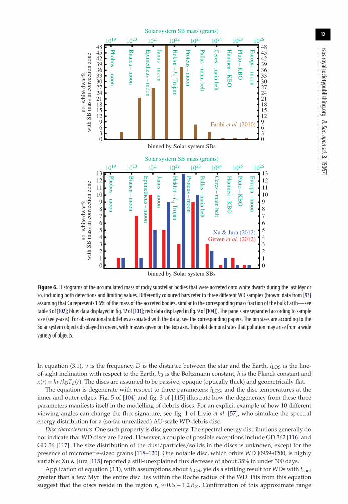
Accumulated metal mass in the convection zone. For DB WDs, the situation is different. Their convectionzones are deep enough to hold a record of all remnant planetary accretion over the last Myr or so. Thisfeature allows us to estimate lower bounds for the total amount accreted over this timescale. Figure 6illustrates the amount of mass in metals, in terms of Solar system asteroids, moons and one L4 JupiterTrojan, that has been accreted in two different WD samples.

Other constraints. Some metal-polluted WDs are magnetic (denoted with an ‘H’ in the spectralclassification). At least 10 DZH WDs harbour magnetic fields of 0.5–10 MG [105], although thispreliminary work indicates this number is likely to be double or triple. The theoretical implications ofmagnetic fields have previously only briefly been touched upon (§12.2).

Further, hydrogen abundance in WD atmospheres, although not considered a ‘pollutant’, neverthelessmight provide an important constraint on pollution. Because hydrogen does not diffuse out of a WDatmosphere, this chemical element represents a permanent historical tracer of accretion throughout theWD lifetime (even if the WD’s spectral type changes as a function of time). Accretion analyses andinterpretations, however, must assume that the WD begins life with a certain amount of primordialH. This accretion arises from a combination of the interstellar medium, asteroids, comets and anyplanets. Of these, comets—and in particular exo-Oort cloud comets—might provide the greatest amountof this hydrogen through ices. Consequently, linking WD hydrogen content with cooling age mayhelp determine the accretion rate of exo-Oort cloud comets soon after the WD is formed [67] andover time [106]. Fig. 5 of [91] illustrates how WD hydrogen mass appears to be a steadily increasingfunction of cooling age, and increases at a rate far greater than realistic estimates of accretion from theinterstellar medium.

3.1.2. White dwarf debris discs

Debris discs have been detected orbiting nearly 40 polluted WDs. The first disc discovered orbits the WDGiclas 29–38 (commonly known as G 29–38) [107] in 1987. Nearly two decades passed before the seconddisc, orbiting GD 362 [108,109], prompted rapid progress. No confidently reported debris disc around asingle unpolluted WD exists, suggesting the link between pollution and discs is strong. At least a fewpercent and up to 100% of all WDs host discs [110–112]. The lower limit for the Galactic population isbased on actually observed discs, whereas the one-to-one potential correspondence between pollutionand the presence of a disc is based on most discs likely being too faint to detect. Although observationalsensitivities allow pollution to be discovered in WDs with tcool as high as about 5 Gyr, discs are difficultto detect for tcool > 0.5 Gyr [112]. Farihi [18] recently summarized observations of these discs. See alsotable 1 of [110], table 1 of [103] and table 2 of [113] for some details of dust-only discs found before 2012.

Detection constraints. All these discs are dusty, and dust comprises the major if not sole component.Consequently, the detection and characterization of the discs rely on modelling spectral energydistributions with a signature (‘excess’ with respect to the flux from the WD) in the infrared and a totalflux, F , prescription that is given in eqn 3 of [114]:

F ≈ 12π1/3 cos (iLOS)R2

�

D2

(2kBT�

3hν

)8/3 hν3

c2

∫ x(out)

x(in)

x5/3

exp(x) − 1dx. (3.1)

12


................................................

48454239363330272421181512

Farihi et al. (2010)9630

484542393633302724211815129630

binned by Solar system SBs

Solar system SB mass (grams)

Phobos–

moon

1019 1020 1021 1022 1023 1024 1025 1026

Bianca

–m

oon

Epim

etheus–

moon

Janus–

moon

Europa

–m

oon

Hektor–

L4 T

rojam

Proteus–

moon

Pallas–

main belt

Ceres

–m

ain belt

Haum

ea–

KB

O

Pluto–

KB

O

no. w

hite

dw

arfs

with

SB

mas

s in

con

vect

ion

zone

Girven et al. (2012)Xu & Jura (2012)

131211109876543210

131211109876543210

binned by Solar system SBs

Solar system SB mass (grams)

Phobos–

moon

1019 1020 1021 1022 1023 1024 1025 1026

Bianca

–m

oon

Epim

etheus–

moon

Janus–

moon

Europa

–m

oon

Hektor–

L4 T

rojan

Proteus–

moon

Pallas–

main belt

Ceres

–m

ain belt

Haum

ea–

KB

O

Pluto–

KB

O

no. w

hite

dw

arfs

with

SB

mas

s in

con

vect

ion

zone

Figure 6. Histograms of the accumulated mass of rocky substellar bodies that were accreted onto white dwarfs during the last Myr orso, including both detections and limiting values. Differently coloured bars refer to three different WD samples (brown: data from [93]assuming that Ca represents 1.6% of the mass of the accreted bodies, similar to the corresponding mass fraction of the bulk Earth—seetable 3 of [102]; blue: data displayed in fig. 12 of [103]; red: data displayed in fig. 9 of [104]). The panels are separated according to samplesize (see y-axis). For observational subtleties associated with the data, see the corresponding papers. The bin sizes are according to theSolar system objects displayed in green, with masses given on the top axis. This plot demonstrates that pollution may arise from a widevariety of objects.

In equation (3.1), ν is the frequency, D is the distance between the star and the Earth, iLOS is the line-of-sight inclination with respect to the Earth, kB is the Boltzmann constant, h is the Planck constant andx(r) ≡ hν/kBTd(r). The discs are assumed to be passive, opaque (optically thick) and geometrically flat.

The equation is degenerate with respect to three parameters: iLOS, and the disc temperatures at theinner and outer edges. Fig. 5 of [104] and fig. 3 of [115] illustrate how the degeneracy from these threeparameters manifests itself in the modelling of debris discs. For an explicit example of how 10 differentviewing angles can change the flux signature, see fig. 1 of Livio et al. [57], who simulate the spectralenergy distribution for a (so-far unrealized) AU-scale WD debris disc.

Disc characteristics. One such property is disc geometry. The spectral energy distributions generally donot indicate that WD discs are flared. However, a couple of possible exceptions include GD 362 [116] andGD 56 [117]. The size distribution of the dust/particles/solids in the discs is unknown, except for thepresence of micrometre-sized grains [118–120]. One notable disc, which orbits WD J0959-0200, is highlyvariable: Xu & Jura [115] reported a still-unexplained flux decrease of about 35% in under 300 days.

Application of equation (3.1), with assumptions about iLOS, yields a striking result for WDs with tcoolgreater than a few Myr: the entire disc lies within the Roche radius of the WD. Fits from this equationsuggest that the discs reside in the region rd ≈ 0.6 − 1.2 R�. Confirmation of this approximate range

13


................................................

750

500

250

0

Vy

[km

s–1

]

Vx [km s–1]

2016–12

2006

–07

2015–06

2012–03

2009–04

–250

–500

–750

750 500 250 0 –250 –500 –75020

03–0

3

2.0R

�

0.2R

�

Figure 7. Exact reproduction of fig. 5 of [122]. This image is a velocity spacemap of the gaseous component of the debris disc orbiting theWD SDSS J1228+1040. The subscripts x and y refer to their usual Cartesianmeanings, and theWD is located at the origin. Observations atparticular dates are indicated by solidwhite lines. The image suggests that the disc is highly non-axisymmetric and precessing on decadaltimescales.

arose with the discovery of both dusty and gaseous components in seven of these discs. The gaseouscomponents constrain the disc geometry. This distance range clearly demonstrates that (i) the discs donot extend all the way to the WD surface (photosphere) and that (ii) the discs could not have formedduring the MS or GB phases. Regarding this first point, some spectral features do suggest the presenceof gas within 0.6R� (e.g. see the bottom-left panel of fig. 3 in [83]), but not yet in a disc form.

The first gaseous disc component found (around SDSS J122859.93+104032.9, also known as SDSSJ1228+1040) [121], also exhibits striking morphological changes, which occur secularly and smoothlyover decades (whereas the disc orbital period is just a few hours) [122] (figure 7). The figure is a velocityspace intensity distribution where the radial white lines indicate different times from the years 2003–2016. Four other discs with time-resolved observations of gaseous components are SDSS J0845+2258,SDSS J1043+0855, SDSS J1617+1620 and SDSS J0738+1835. The first three of these—which change shapeor flux over yearly and decadal timescales—represent exciting dynamical objects, while the last, whichexists in an apparently steady state (given just a handful of epochs so far), might provide an importantand intriguing contrast.

One notable exception to all of the above WD discs is a very wide (35–150 AU) dusty structureinferred orbiting the extremely young (tcool 1 Myr) WD 2226-210 [123]. The interpretation of this dustyannulus representing a remnant exo-Kuiper belt is degenerate and is not favoured compared to a stellarorigin [124]: i.e. this annulus might represent a planetary nebula.

3.2. Major and minor planets around white dwarfs

3.2.1. Orbiting white dwarfs

A few WDs host orbiting SBs, and they are all exoplanetary record-breakers (as of time of writing) in atleast one way.

The fastest, closest and smallest SBs. Transit photometry of WD 1145+017 revealed signatures of one toseveral SBs (with RSB < 103 km) which are currently disintegrating within the WD disruption radius withorbital periods of 4.5–5.0 h [125,126]. Gänsicke [127] have since constrained the orbital periods of at leastsix SBs to within 15 s of 4.4930 h each, indicating almost exactly coplanar and equal orbits. Further, within

14


................................................the same system, Xu et al. [128] have detected circumstellar absorption lines from likely gas streams, aswell as 11 different metals in the WD atmosphere.

Because this WD is both polluted and hosts a dusty debris disc, these minor planet(s) furtherconfirm the interpretation that accretion onto WDs and the presence of circumstellar discs is linkedto first-generation SB disruption (see §9). This type of discovery was foreshadowed by previousprognostications. (i) Soker [129] found that for stars transitioning from the AGB to WD phase, theirshocked winds can create mass ablation from surviving planets into a detectable debris tail. (ii) Villaver &Livio [52] predicted that planets evaporating and emitting Parker winds could be detected withspectroscopic observations, but was thinking of atmospheric mass outflows at several AU around GBstars. (iii) Di Stefano et al. [130] demonstrated specifically that the Kepler space mission should be ableto detect WD transits of minor planets. Ironically, although the paper was written with the primaryKepler mission in mind, only during the secondary mission were enough WDs observed to achieve thisdiscovery. (iv) Alternatively, Spiegel & Madhusudhan [131] claimed that the process of a stellar windaccreting onto an SB might produce a detectable coronal envelope around the SB.

The furthest and slowest exoplanet. WD 0806-661 b is a planetary mass (7MJup) SB orbiting the WD atan approximate distance of 2500 AU [132]. Although some in the literature refer to the object as a browndwarf, the mass is well constrained to be in the planet regime (see fig. 4 of [132]). The difference ofopinions is perhaps partly informed by contrasting assumptions about the SB’s dynamical origin ratherthan its physical properties. The planet was discovered using direct imaging, and holds the currentrecord for the bound exoplanet with the widest orbit known.

The first circumbinary exoplanet. The first successfully predicted [133,134] and confirmed [135]circumbinary exoplanet, PSR B1620-26AB b, orbits both a WD (with mass ≈0.34 M� and cooling ageof approx. 480 Myr) and a millisecond pulsar (with mass ≈1.35 M� and rotation period of 11 ms). TheWD cooling age and pulsar rotation period importantly help constrain the dynamical history of thesystem. The planet’s physical and orbital parameters are MSB ∼ 2.5MJup, a ∼ 23 AU and i ∼ 40◦, whereasthe binary orbital parameters are ab ≈ 0.8 AU and eb ≈ 0.025.

PSR B1620-26AB b is the only known planet in a system with two post-MS stars, and one of thefew exoplanets ever observed in a metal-poor environment and cluster environment (the M4 globularcluster). The planet name contains ‘PSR’ because the pulsar was the first object in the system discoveredand is the most massive object (the primary). However, the planet was originally thought to orbit (andform around) the progenitor of the WD, and hence is more appropriately linked to that star. Further, I donot classify this system as a post-CE binary (see §3.4) because both the system does not fit the definition ofcontaining a WD and a lower-mass MS companion, and the system is typically not included in the post-CE binary literature [136]. This combination of pulsar, WD and planet suggests a particularly fascinatingdynamical history (see §7.3.2).

Hints of detections. In addition to the above observations, there are several hints of SBs orbiting WDs.The magnetic WD GD 365 exhibits emission lines which could indicate the presence of a rocky planetwith a conducting composition [137]. Later data has been able to rule out an SB with MSB ≥ 12MJup [25],which is consistent with the rocky planet hypothesis. Also, the spectral energy distribution of PG0010+280 may be fit with an SB with r ≈ 60 AU [138]. In order for this SB to be hot enough for detection,it may have been re-heated; see their Sec. 3.3.2.

Further, a few tenths of percent of Milky Way WDs host brown dwarf-mass SBs [139]. Thesecompanions were found to orbit at distances beyond the tidal engulfment radius of the AGB progenitorof the WD until the notable discovery of WD 0137-349 B [140]. This brown dwarf has MSB = 0.053 M�.For the primary WD star, M� = 0.39 M�. The orbit is close enough—(a sin iLOS = 0.375R� = 0.0017 AU)—that WD 0137-349 B must have survived engulfment in the GB envelope of the progenitor. The low massof the WD is characteristic of premature CE ejection by a companion.

Search methods. For a recent short summary of the different techniques employed to search for planetsaround WDs, see Section 1 of [141]. The discovery of SBs orbiting WD 1145+017 based on transitphotometry [125] highlights interest in this technique. Faedi et al. [142] placed limits (less than 10%)on the frequency of gas giants or brown dwarfs on circular orbits with orbital periods of several hours,and mentioned that exo-moons orbiting WDs can generate 3% transit depths. An important caveat to thistransit method is that it requires follow-up with other methods, at least according to [143], who wrotethat for WDs, ‘planet detection based on photometry alone would not be credible’.

Existing relevant formulae suppose that the SB is smaller than the star (which is not true for giantplanets or Earth-sized SBs orbiting WDs), and some formulae make other approximations (like circularityof orbits) which would be ill-suited for the type of transits suggested by e.g. [144]. Useful formulae frompost-MS studies are provided by eqns 1–2 of [142], eqn 1 of [145] and eqns 18–19 of [76]. Faedi et al. [142]

15


................................................estimate the depth of the transit to be equal to unity if RSB ≥ R� and, instead, to approximately equalR2

SB/R2� if RSB < R�. The probability of transit and the duration of transit represent other quantities of

interest. I display these by repackaging the fairly general expressions from eqns 9–10 of [146]:

probability =(

R� + RSB

a

)(1 ± e sin ω

1 − e2

), (3.2)

where ω is the argument of pericentre of the orbit, the upper sign is for transits (SB passing in front ofthe WD) and the lower sign is for occultations (or ‘secondary eclipses’, when the SB passes in back ofthe WD). Both formulae assume grazing eclipses, and that eclipses are centred around conjunctions.Maintaining this sign convention, I then combine eqns 7, 8, 14, 15 and 16 of [146] to obtain thetransit/occultation duration:

duration = 2

( √1 − e2

1 + e sin ω

)√a3

G(M� + MSB)

× sin−1

⎡⎣ R�

a sin iLOS

{(1 ± RSB

R�

)2− a2 cos2 iLOS(1 − e2)2

R2�(1 + e sin ω)2

}1/2⎤⎦ , (3.3)

where iLOS is the inclination of the orbit with respect to the line of sight of an observer on the Earth. Byconvention, an edge-on orientation corresponds to iLOS = 90◦.

3.2.2. Orbiting the companions of white dwarfs

Three stellar systems are known to harbour a planet-hosting star and a WD: GJ 86, ε Reticulum (or ε

Ret), and HD 147513. In no case is the WD (yet) known to be polluted nor host debris discs, planets orasteroids.

The star GJ 86B is an unpolluted WD [147] whose binary companion GJ 86A is an MS star thathosts a MSB � 4.5MJup planet in an a = 0.11 AU orbit [148,149]. With Hubble Space Telescope data, Farihiet al. [147] helped constrain the physical and orbital parameters of the system (see their table 4), whichfeatures a current binary separation of many tens of AU. The planet GJ 86Ab survived the GB evolutionof GJ 86B, when ab expanded by a factor of a few, but eb remained fixed (see §4).

A similar scenario holds for the HD 27442 system. The star ε Ret, or HD 27442A, hosts a MSB �1.6MJup planet in a a = 1.27 orbit [150]. The projected separation between ε Ret and its WD binarycompanion, HD 27442B, is approximately a couple hundred AU [151]. The HD 147513 system is notas well constrained [152]. However, the separation between the binary stars in that system is thoughtto be several thousand AU, placing it in the interesting ‘non-adiabatic’ mass loss evolutionary regime(equation (4.10)).

3.2.3. White dwarf–comet collisions

In the 1980s, the potential for collisions between exo-comets and their parent stars, or other stars, toproduce observable signatures was realized [153–155]. Alcock et al. [156] more specifically suggested thatcomet accretion onto WDs can constrain number of exo-Oort cloud comets in other systems. Pineault &Poisson [155] and Tremaine [157] included detailed analytics that may still be applicable today. Some ofthis analysis was extended to binary star systems in Pineault & Duquet [158], with specific application tocompact objects in their Sec. 4.3. Perhaps, these speculations have been realized with the mysterious X-ray signature from IGR J17361-4441 reported in Del Santo et al. [159], although that potential disruptionevent may also have just been caused by planets or asteroids rather than comets.

3.3. Subgiant and giant star planetary systems

3.3.1. Giant branch planets

Gross characteristics. As of 30 Nov 2015, 79 SBs were recorded in the planets-around-GB-stars database1,although this number may be closer to 100 [160]. About 85% of these SBs are giant planets with MSB ∼ 1 −−13MJup, proving that planets can survive over the entire MS lifetime of their parent stars. The host starsfor these SBs have not undergone enough GB evolution to incite mass loss or radius variations which aremarkedly different from their progenitor stars. These barely evolved host stars are observed in their early

1Sabine Reffert maintains this database at www.lsw.uni-heidelberg.de/users/sreffert/giantplanets.html.

16


................................................RGB phase, sometimes known as the ‘subgiant’ phase. Because RGB tracks on the Hertzprung–Russelldiagram are so close to one another, RGB masses are hard to isolate; there is an ongoing debate over thesubgiant SB-host masses [161–166].

Regardless, the population of these SBs shows a distinct characteristic: a paucity of planets (less than10%) within half of an AU of their parent star. In contrast, a < 0.5 AU holds true for about three-quartersof all known exoplanets. This difference highlights the need to better understand the long-term evolutionof planetary systems. Further, a handful of GB stars have been observed to host multiple planets. Thesesystems may reveal important constraints on dynamical history. For example, the two planets orbitingη Ceti may be trapped in a 2:1 mean motion resonance (see the fourth and fifth rows of plots in fig. 6of [167]). A resonant configuration during the GB phase would help confirm the stabilizing nature of (atleast some types of) resonances throughout all of MS evolution.

Regarding the planet–giant star metallicity correlation, Maldonado et al. [168] and Reffert et al. [169]arrived at somewhat different conclusions. The former concluded that planet-hosting giant stars arepreferentially not metal rich compared to giant stars that do not host planets. The latter, using a differentsample, showed that there was strong evidence for a planet—giant star metallicity correlation.

Lithium pollution? One case of particular interest is the BD+48 740 system [37], which contains both(i) a candidate planet with an unusually high planet eccentricity (e = 0.67) compared with other evolvedstar planets and (ii) a host star that is overabundant in lithium. Taken together, these features aresuggestive of recent planet engulfment: Lillo-Box et al. [10] wrote: ‘The first clear evidence of planetengulfment’. They also helped confirm existence of the MS planet Kepler-91b, a tidally-inspiralingextremely close-in planet with r ≈ 1.32R�, and estimate that its fate might soon (within 55 Myr) mirrorthat of the engulfed planet in BD+48 740.

Transit detection prospects. In principle, SBs may be detected by transits around GB stars. Theapplication of equations (3.2 and 3.3) to this scenario is interesting because, as observed by Assefet al. [170], despite the orders of magnitude increase in stellar radius from the MS to GB phases, thereis a corresponding increase in values of a for surviving SBs. Therefore, the transit probability shouldnot be markedly different. The equations neglect however, just how small the transit depth becomes:R2

SB/R2� ∼ 10−5.

3.3.2. Giant branch debris discs

Importantly, planets are not the only SBs that survive MS evolution. Bonsor et al. [171] revealed the firstresolved images of a debris disc orbiting a 2.5 Gyr-old subgiant ‘retired’ A star (κ Coronae Borealis or κ

CrB), although they could not distinguish between one belt from 20 to 220 AU from two rings or narrowbelts at about 40 and 165 AU. This finding demonstrates that either the structure survived for the entiremain sequence lifetime, or underwent second-generation formation. This discovery was followed upwith a survey of 35 other subgiant stars, three of which (HR 8461, HD 208585 and HD 131496) exhibitinfrared excess thought to be debris discs [172]. Taken together, these four disc-bearing GB stars suggestthat large quantities of dust could survive MS evolution.

3.4. Putative planets in post-common-envelope binariesSome binary stars which have already experienced a CE phase are currently composed of (i) either a WDor hot subdwarf star, plus (ii) a lower-mass companion. These binaries are classified as either ‘detached’or ‘semi-detached cataclysmic variables’ depending on the value of rb. Over 55 of these binaries havejust the right orientation to our line of sight to eclipse one another. These systems are known as post-CE binaries. The eclipse times in these binaries should be predictable if there are no other bodies in thesystem and if the stars are physically static objects.

In several cases, this idealized scenario has not been realized, allowing for the exciting possibilityof exoplanet detections. Zorotovic & Schreiber [136] reviewed the potential origin of eclipse timingvariations for all known post-CE binaries (see their table 1 and appendix A), and emphasized that‘extreme caution’ must be exercised when evaluating a first-generation origin for these putative planets.The reason is that binary stars are complex structures and can mimic planetary signals. Of the 12 systemshighlighted in that table for potentially hosting planets or brown dwarfs, the existence of these SBsremain in doubt due to stability analyses (see §7.4). For SBs which are thought to exist, their dynamicalorigin remains in question. Section 5 of [136] discusses the possibility of second-generation formation;see also §8 of this paper.

17


................................................The most robust detections are the putative planets around the post-CE binary NN Serpentis, or NN

Ser. Beuermann et al. [173,174] found excellent agreement with a two-planet fit, and found resonantsolutions with true librating angles [174]. A recent analysis of 25 years worth of eclipse timing datafor this system (see fig. 2 of [175]) strengthens the planetary hypothesis, particularly because timingsbetween the years of 2010–2015 matched the predicted curve. They do not, however, claim that theseplanets are confirmed, because there still exists a degeneracy in the orbital solutions. In fact, Mustillet al. [176] provided evidence against the first-generation nature of these planets by effectively backwardsintegrating in time to determine if the planets could have survived on the MS. The largest uncertainty intheir study is not with the orbital fitting but rather how the CE evolved and blew off in that system.

If confirmed, other reported systems which may be dynamically stable would prove exciting.However, pulsation signals, which are intrinsic to the parent star, can mask timing variations that wouldotherwise indicate the presence of SBs (e.g. [177]). Charpinet et al. [178] detected signals around the hotsubdwarf star KIC 05807616 which could correspond to SBs with distances of 0.0060 and 0.0076 AU.Silvotti et al. [179] instead detected timing variations around the subdwarf pulsator KIC 10001893 withperiods of 5.3, 7.8 and 19.5 h.

3.5. Pulsar planetsPulsar arrival timings in systems with a single pulsar are generally better constrained than those in post-CE binaries because pulsars are more reliable clocks than WD or MS stars, and radiation from a singlesource simplifies the interpretation. Identifying the origin of residual signals for millisecond pulsars iseven easier.

These highly precise cosmic clocks, combined with a fortuitous spell of necessary maintenancework on the Arecibo radio telescope, provided Alexander Wolszczan with the opportunity to find PSRB1257+12 c and d [1] (sometimes known as PSR B1257+12 B and C), and eventually later PSR B1257+12 b(sometimes known as PSR B1257+12 A) [2]. Wolszczan [180] detailed the history of these discoveries. Notincluded in that history is how the identities of the first two planets were almost prematurely leaked bythe British newspaper The Independent in October 1991 [181]. The article referred to these planets as ‘onlythe second and third planets to be found outside our own solar system’ because of the ironic assumptionthat the first-ever exoplanet was the (later-retracted [182]) candidate PSR 1829-10 b.

The observed and derived parameters for the PSR B1257+12 system remain among the bestconstrained of all exoplanets (see table 1 of [180]), with eccentricity precision to the 10−4 level, a valuefor the mutual inclination of planets c and d (which is about 6 degrees), and a derived mass forplanet b of 0.020 M⊕ = 1.6MMoon. However, these values are based on the assumption that M� = 1.4 M�.PSR B1257+12 b has the smallest mass of any known extrasolar SB, given that we do not yet havewell-constrained masses for the (disintegrating) SBs orbiting WD 1145+017. The other two planets are‘super-Earths’, with masses of planets c and d of 4.3M⊕ and 3.9M⊕. All three planets lie within 0.46 AUof the pulsar and travel on nearly circular (e < 0.026) orbits. The orbital period ratio of planets b and c isabout 1.4759, which is close to the 3:2 mean motion commensurability.

I have already described the one other bona-fide planet discovered orbiting a millisecond pulsar,PSR B1620-26AB b, in §3.2.1, because that planet also orbits a WD. For an alternative and expandedaccounting of this planet as well as the PSR B1257+12 system, see the 2008 review of neutron star research[183].

Pulsar planets are rare. A recent search of 151 young (<2 Myr old) pulsars (not ms pulsars) with theFermi telescope yielded no planets for MSB > 0.4M⊕ and with orbital periods of under 1 year [184]. Theauthors used this result as strong evidence against post-SN fallback second-generation discs (see §8.2),particularly because theoretical models constrain these discs to reside within about 2 AU.

3.6. Circumpulsar asteroid and disc signaturesSometimes the deviations in pulse timing are not clean in the sense that they cannot be fit with one or afew planets or moon-sized SBs. Rather, the deviations may be consistent with other structures, such asdiscs, rings, arcs or clouds. Wang [185] recently reviewed observational results from debris disc searchesaround single pulsars.

The residuals for the millisecond pulsar B1937+21 are consistent with an asteroid disc of mass lessthan about 0.05 M⊕ [186], and with constrained properties given in their table 2. Asteroids can affectthe timing precision of received signals from millisecond pulsars down to the ns level. Their fig. 5nicely compares their sensitivity limits for asteroids in PSR B1937+21 with the PSR B1257+12 planets.

18


................................................Unfortunately, the asteroids interpretation is degenerate with other possibilities, and difficult to test (seetheir section 7).

Previously, Lazio et al. [187] and Löhmer [188] placed limits on the masses of dust discs in othermillisecond pulsars. However, unlike for PSR B1937+21, these other pulsars did not have timingresiduals that were fit to specific asteroid belt or disc architectures [186]. Bryden et al. [189] searched for adust disc in PSR B1257+12, but were not able to exclude the presence of a Solar system-like asteroid beltwith a mass as large as 0.01M⊕ and SBs with radii up to 100 km. The X-ray pulsar or young magnetar4U 0142+61 might host a disc [190,191], although the infrared excess in that system instead could beexplained by magnetospheric emission [192]. Also, anomalous timing and radio emission signaturesof the pulsar PSR J0738-4042 [193] cannot be explained by known stellar evolutionary processes. Suchabrupt changes can be caused by encounters with asteroids, as argued by the authors.

Cordes & Shannon [194] expect asteroids to enter pulsar magnetospheres and create the largestdetectable signals for large spin periods, large spin-down ages, large magnetospheres, low surfacetemperatures and low non-thermal luminosities (see their fig. 1). They also posed that interstellar cometsimpacting with circumpulsar discs may produce observable episodic behaviour. They stated that foran AU-scale dense disc with a high optical thickness, events may occur at the rate of once per year.Mitrofanov [195] postulated that these events may produce gamma ray bursts and prompt a ‘re-ignition’of the pulsar.

4. Stellar mass ejectaHaving motivated the study of post-MS planetary systems, I now turn to important forces in thesesystems. Stellar mass loss is arguably the most important driver of all post-MS forces because it non-negligibly affects the orbits of all SBs at all distances (figure 2). In this vein, the classical mechanics-basedmass-variable two-body problem has gained renewed importance with the mounting discoveries of post-MS planetary systems. For decades, this same problem has been relevant and applicable to binary stars,which represented the physical picture envisaged by early (pre-exoplanet era) studies.

The mass variable two-body problem is dynamically rich and not energy conserving. The problem canbe broken down into the following questions: (i) How many bodies are losing mass? (ii) Is the mass lossisotropic? (iii) Is the mass loss instantaneous? (iv) Does a natal kick accompany the mass loss? (v) Arethe bodies assumed to be point masses? (vi) How are one or both bodies dragged through the ejecta?These questions are not mutually exclusive, complicating a straightforward presentation. I proceed bygrouping the first four questions into §4.1, the fifth question into §4.2 and the last question into §4.3.

4.1. The mass-variable point-mass two-body problemPublished investigations of the problem itself date back to the late nineteenth century: Razbitnaya [196]provided a brief historical review. Table 1 of that paper exhaustively lays out the equations of motionin 22 different cases, depending on the reference frame, relative velocities, whether one or both of themasses is variable, and whether the mass loss is isotropic. In all cases, both bodies are assumed to bepoint masses. For most post-MS planetary science applications, when the SB mass is considered fixed,rows #6 (anisotropic mass loss) and #7 (isotropic mass loss) of that table provide the relevant equations.When the SB itself is shedding mass (perhaps due to atmospheric evaporation; see §6.1.2 of this paper)or when its accreting the mass ejected from the star, then the equations in rows #1 (anisotropic mass loss)and #2 (isotropic mass loss) should instead be used.

4.1.1. Isotropic mass loss set-up

In the most general point-mass isotropic mass loss case where both bodies are losing mass (row #2), theequation appears to be no different from the fixed masses case:

d2rdt2 = −G(M� + MSB)

r3 r. (4.1)

What is different is that both masses are functions of time. In order to help understand the implicationsand provide physical intuition for their meaning, John D. Hadjidemetriou and Tuken B. Omarovindependently, and using different approaches in different languages, derived in 1962–1963 thecorresponding equations of motion for isotropic mass loss in planetary orbital elements [197,198]. Thelack of internet and political considerations in the early 1960s prevented the eventual good friends fromknowing about each other’s work until long after.

19


................................................Both Hadjidemetriou and Omarov realized that equation (4.1) may be expressed as

d2rdt2 = −G(M�(t = 0) + MSB(t = 0))

r3 r − 12(M�(t) + MSB(t))

d(M�(t) + MSB(t))dt

r, (4.2)

such that the classic orbitally static two-body problem is perturbed by a single mass loss term. Isolatingthis term helps quantify the motion. Equation (4.2) is derived from equation (4.1) by determining thetotal derivative of velocity with respect to time. This derivative is the sum of the partial derivative with(M� + MSB) held constant, plus the partial derivative with r held constant. The results of their derivationsof the equations of motion entirely in terms of planetary elliptical orbital elements are as follows. I writethem in terms of both true anomaly f and eccentric anomaly E:

dadt

= − a(1 + e2 + 2e cos f )1 − e2

M� + MSB

M� + MSB= −a

(1 + e cos E1 − e cos E

)M� + MSB

M� + MSB, (4.3)

dedt

= −(e + cos f )M� + MSB

M� + MSB= −

[(1 − e2) cos E

1 − e cos E

]M� + MSB

M� + MSB, (4.4)

didt

= 0 = 0, (4.5)

dΩ

dt= 0 = 0 (4.6)

anddω

dt= −

(sin f

e

)M� + MSB

M� + MSB= −

[√1 − e2 sin E

e(1 − e cos E)

]M� + MSB

M� + MSB. (4.7)

Here Ω and ω refer to the longitude of ascending node and argument of pericentre. In order to completethe sets, the evolution of the anomalies themselves are

dfdt

= −dω

dt+ n(1 + e cos f )2

(1 − e2)3/2 (4.8)

anddEdt

= − 1√1 − e2

dω

dt+ n

1 − e cos E. (4.9)

In these equations, n = G1/2(M� + MSB)1/2a−3/2 represents the mean motion. Between the mid-1960s andthe 2010s, these relations have not appeared often in other literature. One notable example is Alexanderet al. [199], whose equations (3.11)–(3.13) can be reduced to the above relations. Equation (4.3) illustratesthat the semi-major axis always increases due to isotropic mass loss. Together equations (4.3) and (4.4)may be combined to show that the orbital pericentre also always increases. The argument of pericentreis not defined for circular orbits and changes rapidly for near-circular orbits.

As observed by Adams et al. [200], a danger of using osculating Keplerian orbital elements is theinterpretation of their non-Keplerian time evolution: for example, apparent oscillations in e can maskthe motion’s actual smooth spiral. Iorio [201] further emphasized the importance of considering the timeevolution of all the orbital elements concurrently to obtain a true picture of the motion. An alternativeway of describing the motion is through a radial equation of motion [202]. Adams et al. [200] recentlydeveloped a dimensionless form of this equation and derived resulting relations for time-dependentmass-loss prescriptions in this framework.

4.1.2. Anisotropic mass loss set-up

Equations (4.3)–(4.9) assume that the mass is lost isotropically. If one removes this assumption, andmodels direction-dependent mass loss and differential mass ejecta speeds, then additional terms appearin the equations. These terms are given by eqns 34–38 of [203]2 and are expressed in terms of mass fluxrelations from their eqn 4. These modified equations demonstrate that (i) the inclination and longitude ofascending node do change with time, and that (ii) anisotropy becomes more important the further awayan SB is, as the anisotropic terms contain an additional factor of

√a. Veras et al. [203] proved that mass-

loss variations must be asymmetric about the stellar equator in order to affect the motion of SBs. They

2Appropriately, after a distinguished career pioneering the dynamical field of periodic orbits, Hadjidemetriou returned to the topicof mass loss, and in his final paper [203] helped derived the anisotropic mass loss equations of motion and applied them to pre-and post-MS planetary systems. Confirmation of some of these equations can be found in Omarov’s work [197] in his eqn 13. ForEnglish-language context, see also eqns 19–24 of [204].

20


................................................showed that for most post-MS applications with SBs within a few hundred AU, isotropy is an excellentapproximation.

Although motivated by atmospheric evaporation on the MS, the mass loss formalisms presented by[205,206] provide potentially useful alternative approaches. Iorio [205] expressed the mass loss term inradial and tangential components, and then applied the Gaussian equations in that coordinate system;a variation on Omarov’s approach [197]. Boué et al. [206] instead treated radial mass loss from a solidangle patch of the atmosphere of one body (different from the one-dimensional jets from [203]) so thatthe mass emanates in a conical shape.

Parriott & Alcock [207] modelled anisotropy of mass loss in a different manner: through a kick, or avelocity impulse, of the star. Their equations of motion (in their eqn 1, which must contain a typographicerror) include a term which requires a priori knowledge of the star’s final (WD) mass given a velocityimpulse prescription.

4.1.3. Isotropic non-instantaneous mass loss solutions

Veras et al. [208] extensively analysed equations (4.3)–(4.9), and observed that they can be derivedvia either perturbation techniques or the vis viva equation, combined with conservation of angularmomentum expressed in polar coordinates. They also found importantly that the osculating pericentremonotonically increases with mass loss (their eqn 21), regardless of the mass loss prescription chosen.Although early studies like Hadjidemetriou [209] used the equations to show that orbital eccentricitychanges are triggered by high mass loss, even for an initially circular orbit, the mounting observations ofpost-MS systems have led to a renewed interest in this problem.

Parametrizing solutions. Equations (4.3)–(4.9) do not appear to have a complete analytical solution.They do, however, admit two well-defined solution regimes and a difficult-to-characterize transitionregime. In order to identify these solution regimes, consider the (dimensionless) scaled ratio of thetimescales of orbital period to mass loss

Ψ ≡ M�

M�n= 1

2π

(M�

M� yr−1

)(M�

M�

)−3/2 ( aAU

)3/2. (4.10)

When Ψ 1, the system is commonly said to be in the ‘adiabatic’ regime. When Ψ 1, the system is ina regime without a widely used moniker. The transition regime lies between these two extremes, and Ψ

itself changes with time (eqn 16 of [208]) so that if mass loss continued indefinitely, the system wouldenter the Ψ 1 regime from the adiabatic regime. The term ‘adiabatic’ in this context does not referto heat, but rather conservation of eccentricity. The reason is that when Ψ 1, the right-hand-sides ofequations (4.4) and (4.7) may be approximated as zero. Further, in this limit, equation (4.3) simplifies to:da/dt = −(M� + MSB)−1(dM�/dt).

As indicated by the maximum mass loss rates in figure 3 and equation (4.10), Ψ 1 for thevast majority of known exoplanets (because a < 100 AU and M(MS)

� ≤ 3 M� in almost every case).Consequently, these exoplanets will expand, but not stretch, their osculating orbits during post-MS massloss by a factor approximately equal to (M(MS)

� /M(WD)� ). During this process, Ψ remains much less than

unity.Critical angles. However, exo-Oort clouds, exo-scattered discs and some exoplanets (like WD 0806-

661 b from [132]) have a more complex post-MS fate. For these systems, either Ψ ∼ 1 or Ψ 1. In thelatter case, special solutions of the equations of motion exist, as outlined in section 2.6.2 of [208]. Relatedfundamental properties of the two-body problem derived in section 2.5 of [208] are the two critical trueanomalies fcrit

fcrit ≡ π ± 12

cos(

79

)≈ 160.5◦ and 199.5◦ (4.11)

at which the orbital eccentricity incurs an initial decrease at the onset of mass loss. Consequently, thesevalues mark the boundaries at which some eccentric SBs for Ψ 1 are protected from escape (fig. 16of [208] and figs 9–10 of [210]).

Transition to non-adiabaticity. Based on angular momentum conservation, non-adiabatic motion doesnot ensure that the expansion of the semi-major axis proceeds faster than the adiabatic rate unless theorbit is initially circular (see eqns 1–3 of [176]). The transition regime can be wide in extent, spanningan order of magnitude in a(MS) (see e.g. the bottom two panels in fig. 10 of [210]). In the top panel, themass loss is strong enough to ensure Ψ 1. For the most non-adiabatic of all the plots in that top panel(bottom-rightmost plot), the analytic values of fcrit well predict which systems eventually feature escape.

21


................................................Debes & Sigurdsson [211] mentioned an important caveat to the adiabatic transition: the mass loss rate

(from the orbit, and not the star) is dictated by the asymptotic wind velocity and not the ejection velocity.If, at Oort cloud distances, this speed is several orders of magnitude less than the escape speed, thenthe lower wind crossing time effectively decreases the mass loss rate. Consequently, Ψ might decreaseenough for the evolution to still be adiabatic.

Mass loss prescriptions. Up until now, I have not assumed a particular analytic form for the mass lossprescription. Real stars do not follow simple prescriptions, particularly if they lose significant mass onboth the RGB and AGB and pulse violently. Regardless, separately each branch has been fit to linear orexponential forms. Very early work from the 1890s [212,213] assumed dependencies with time. In 2009,Rahoma et al. [214] summarized (in their section 3) different mass-loss prescriptions used throughout theliterature.

More recently, fig. 4 of [215] provided a comparison of the eccentricity excitation due to both linearand exponential mass loss, supposing the same total amount of mass lost. Adams et al. [200] adopted adimensionless mass loss prescription index dependence, and used it to derive an explicit criterion for SBescape (see their eqn 86).

A Hamiltonian framework. Rahoma et al. [214] also treated the point-mass two-body non-instantaneousmass loss problem in the Hamiltonian framework. In their section 2, they provided a brief historicalreview of the problem with many references not listed here. One such reference is the classicallyentertaining paper of Deprit [216], which discusses, among other topics, time-dependent Delaunaytransformations.

4.1.4. Isotropic instantaneous mass loss solutions

Now consider the limit Ψ → ∞, which is relevant (although technically not ever realized) for SNs. Anadvantage of modelling ‘instantaneous’ or ‘impulsive’ mass loss is that no assumptions about mass lossrates nor wind speeds are necessary: Hadjidemetriou [209] showed in this case how the stability of thesesystems crucially depends on the true anomaly at mass loss, with periastron and apastron being thelimiting cases. Nevertheless, a SN process often creates a velocity ‘kick’ from asymmetries within theexploding star. The link between the mass lost and the magnitude and direction of the kick is unclear.Therefore, one best treat the general case of impulsive mass lost plus an arbitrary kick velocity equal tov(NS) − v(MS), which reduces to the mass-loss only situation in the limit of a zero-kick velocity.

Early treatments of this problem [217,218] predate confirmed exoplanets and were motivated by apotential pulsar planet at the time. Both studies, in 1970, considered the effect of instantaneous mass losson a planet’s orbit due to a SN. Only 13 years later, however, was a comprehensive and general treatmentpresented [219].

Explicit expressions. Hills [219] used angular momentum and energy conservation, and theassumptions of instantaneous mass loss from a point-mass MS star, to provide explicit expressionsfor a(NS), e(NS) and the critical value of M(NS)

� /M(MS)� for which the SB escapes, in terms of only MS

orbital parameters (including the true anomaly f ). The expressions for the semi-major axis and massratio include an arbitrary kick, but the eccentricity expression does not because an additional degree offreedom would have to be introduced (see his section IIIb of [219]). By repackaging his eqn 13, includingan arbitrary kick, I obtain

a(NS) =[

a(MS) M(NS)� + MSB

M(MS)� + MSB

]

×⎡⎣1 −

2(

1 + e(MS) cos f (MS))

1 − e(MS)2

(M(MS)

� − M(NS)�

M(MS)� + MSB

)− a(MS)(v(NS)2 − v(MS)2

)

G(M(MS)� + MSB)

⎤⎦

−1

, (4.12)

which I have written in a form that illustrates how the adiabatic approximation (first square brackets) ismodified. The SB will escape the system if, including an arbitrary kick (eqn 15 of [219])

M(MS)� − M(NS)

� >

[M(MS)

� + MSB

2

](1 − e(MS)2

1 + e(MS) cos f (MS)

)(1 − a(MS)(v(NS)2 − v(MS)2

)

G(M(MS)� + MSB)

). (4.13)

I write equation (4.13) in a form which illustrates how the oft-used notion that half of the original mass(in square brackets) must be lost for escape to occur is modified by other parameters. For high values of

22


................................................e(MS), this modification may be severe (see fig. 12 of [208]). In equations (4.12 and 4.13), the expression

v(NS)2 − v(MS)2may be replaced by an expression with the kick velocity, kick angle and v(MS). The final

eccentricity, without an arbitrary kick, is the following repackaged form of their eqn 6:

e(NS)2 = 1 − (1 − e(MS)2)

×[

M(NS)� + MSB

M(MS)� + MSB

]−2 [1 − 2

(M(MS)

� − M(NS)�

M(MS)� + MSB

)(1 + e(MS) cos f (MS)

1 − e(MS)2

)]. (4.14)

Modern re-derivations. Later studies have attempted to reproduce special cases of equations (4.12)–(4.14), without kicks, and typically under the (usually secure) assumption that MSB M�. Veraset al. [208] provided the mass ratio boundedness condition in this case in their eqn 48, except the signof their inequality should be flipped. Even with the above assumption, the expressions for the mass ratioand final eccentricity in eqns 1–2 of [220] do not appear to exactly agree with a reduction of the equationsfrom [219]. Other, alternative formulations of the orbital evolution resulting from SN kicks have beendeveloped (see, e.g. appendix A of [221]).

Equations (4.12)–(4.14) are useful because they are explicit closed equations for which functionaldependencies can quickly be read off. However, if one wished to apply impulsive mass loss together witha kick in an arbitrary Cartesian direction, and derive the post-kick orbital elements, one could instead usethe relations in appendix B of [67]. In the most general case, where the system is in an arbitrary frame, theequations in appendix A of [222], along with those in their section 2, provide a starting point for derivingexplicit expressions of post-kick elements.

4.2. The mass-variable solid body two-body problemSo far, the vast majority of post-MS planetary investigations have treated orbital changes due to stellarmass loss assuming that the SB is a point mass. However, as models become more detailed and take intoaccount physical changes to SBs, one may wish to lift the point mass assumption.

4.2.1. Orbital evolution

If the SB is treated as a solid body, then it will increase in mass through accretion by the stellar wind.Consequently, equation (4.1) is no longer strictly usable. Because mass is no longer ejected from the orbitin the direction of the SB, the mass loss becomes anisotropic, leading to more complex equations (§4.1.2).Hadjidemetriou [198] derived compact expressions in his eqn 44 for how the orbital motion wouldchange in this case, but assumed that the ejecta was moving at the speed of light, and did not accountfor gravitational focusing. In any case, incorporating solid body accretion into the orbital equations ofmotion would need to account for both extra terms in the equations of motion and the time-dependentchange in the SB mass.

4.2.2. Physical evolution

The level of accretion onto the SB itself might be significant. Small enough SBs like pebbles might accretean amount of mass so great that the pebble might be transformed into a boulder, or just be destroyed.Large SBs like planets with atmospheres could have the composition and nature of those atmospherespermanently altered.

What is the accretion rate onto the SB? The literature is replete with answers to this question. Manyanswers differ depending on whether the authors assumed, for example, that gravitational focusing isimportant, the SB is on a circular orbit, and the wind speed is much greater than v. Some expressionsinclude an explicit dependence on M�, whereas others instead show a dependence on ρwind. Thesetwo important quantities are often related through a constant-velocity spherically symmetric (isotropic)mass loss assumption, and when the ‘ejected mass is stratified in concentric spherical layers of constantdensity’ [209]. Consequently (his eqn 2)

ρwind = M�

4πr2|vwind| . (4.15)

By using equation (4.15), one may compare different expressions for MSB which appear in the literature.These include eqn 2 of [223], eqns 1–2 of [224], eqn 1 of [225], eqn 11 of [226] and eqn 4 of [131].

23


................................................The formulation from [221] is expressed in terms of e: repackaging their eqns 6–9 gives

⟨dMSB

dt

⟩= −dM�

dt3

4a2√

1 − e2

(GMSB

v2wind

)2 [1 + G2(M� + MSB)2

a2v2wind

]−3/2

. (4.16)

By using expressions for the accretion rate onto the SB some authors [131,223,224], then estimated thetotal mass accreted by the SB. However, doing so necessitates integrating with respect to time, and M�

is a non-monotonic function of time, initial mass and metallicity along the GB. Nevertheless, Spiegel &Madhusudhan [131] found that brown dwarfs and large planets could accrete an amount of mass that isa multiple of their MS atmospheric masses.

4.3. Stellar wind/gas/atmospheric dragUp until now, I have neglected the physical interaction between the ejected stellar mass and the SB.This assumption might be good for large SBs like planets, and/or tenuous stellar winds. However, fortypical GB stars, the interaction between the stellar wind and smaller SBs like pebbles or asteroids maybe significant. I also include here the treatment of SBs within stellar atmospheres. Although strictly notunder the umbrella of ‘stellar ejecta’, stellar atmospheres provide a similar medium within which dragtakes place, just with a (typically) higher density than the stellar wind. Both the wind and atmosphereare considered to be gaseous media.

4.3.1. Physical evolution

Sufficiently small SBs are in danger of catastrophically disrupting due to ram pressure. For spherical SBswhich are hydrostatic, isothermal and self-gravitating, eqn 1 of [226] provides the following conditionfor stability against disruption:

gSB � 2πρSBρwindv2

RSB(ρ2SB − ρ2

wind), (4.17)

where g is surface gravity. They then specialize to the case ρSB ρwind and g ≈ GMSB/R2SB. These

simplifications yield the following range of masses for which disruption would occur (their eqn 2).I rewrite this equation first from the perspective on atmospheric infall and then for GB winds outsideof the atmosphere:

MSB � 0.02M⊕(

ρwind

10−4 g cm−3

)3/2 (ρSB

2 g cm−3

)−2 (v

100 km s−1

)3(4.18)

∼ 100 kg(

ρwind

10−16 g cm−3

)3/2 (ρSB

2 g cm−3

)−2 (v

10 km s−1

)3. (4.19)

Although approximate, equation (4.18) suggests that giant planets and brown dwarfs should survivecatastrophic disruption while inside stellar atmospheres, and equation (4.19) suggests that asteroids,comets, planets and brown dwarfs will easily survive stellar winds. The situation for boulders andpebbles requires further analysis: Jura [224] assumes that an SB ‘is destroyed if it encounters its ownmass in the wind’ due to hydrodynamic friction, whereas Dong et al. [227] claimed that when the dragforce exceeds the parent star gravitational force, then the SB is ‘entrained’ by the wind.

4.3.2. Orbital evolution

Context for drag. Surviving SBs will have their orbits altered by interactions with the surroundingmedium. The existing post-MS planetary literature has used a variety of names and expressions for theresulting forces. I group the forces into two categories: one consisting of a purely gravitational force dueto the wake generated, and one due to friction. I refer to the former as ‘gravitational drag’ and the latter as‘frictional drag’, in line with Villaver and colleagues [225,228]. Willes & Wu [46] and Rybicki & Denis [229]referred to the frictional drag as ‘bow shock drag’. Schröder & Smith [230] referred to the combinedeffects of gravitational drag and frictional drag as ‘dynamical friction’. In combined expressions, dragterms containing G typically refer to gravitational drag and those without G refer to frictional drag.Schröder & Smith [230] suggested that within the atmosphere, if v ≈ (2 − 3)vsound, where vsound is thesound speed, then both gravitational drag and frictional drag play nearly equal roles.

Gravitational drag. However, gravitational drag is negligible outside of a stellar atmosphere.Consequently, the seminal pre-exoplanet era gravitational drag study of Alexander et al. [199] defined

24


................................................a type of cutoff in their eqn 2.1. Goldstein [231] claimed that this value is ‘usually defined as the neutralpoint between planet and star’, whereas Livio [232] took this value as ‘the mean radius of the planet’sRoche lobe’ and went on to derive analytical relations with this assumption. Alexander et al. [199] thenused their gravitational drag expression and parametrized vwind into radial and tangential componentsin order to derive evolution equations in orbital elements (their eqns 3.11–3.13). These equations alsocontain isotropic mass loss terms and are sufficiently general to reduce to my equations (4.3)–(4.7) in theappropriate limits.

In a seminal later study, Ostriker [233] used time-dependent linear perturbation theory to derive anexpression for the gravitational drag force, which she denotes the ‘dynamical drag force’. This expressionhas subsequently been used for post-MS planetary system applications by others [225,228,230]. For Machnumbers of interest within the atmospheres of GB stars both eqn 5 of [225] and eqn 4 of [228] give

F(grav)drag = 2πG2M2

SBρwind

v2sound

, (4.20)

where F denotes force and ρwind is the density of the atmosphere. Combining equation (4.20) withequation (4.15) would not be appropriate in this context because the star need not be losing mass.Schröder & Smith [230] state that a typical value of vsound within the stellar chromosphere is about8 km s−1. In their study on SB engulfment into GB stars, Villaver & Livio [225] found that v/vsound >

3 always. They adopted vwind = 5 km s−1, whereas Mustill et al. [176] adopted a wind speed of10–15 km s−1. In general, vwind ∝ M� (footnote #1 in [230]).

Frictional drag. The frictional drag force has appeared in several different forms in the post-MSliterature: (i) eqn 6 of [225] and eqn (4) of [228], (ii) eqn 3 of [227] and (iii) eqns 37–39 of [234].The last of these references considers both the Epstein and Stokes regimes of motion, given respectivelyby the upper and lower relations in:

F(fric)drag =

⎧⎪⎪⎪⎨⎪⎪⎪⎩

(MSBρwindvsound

ρSBRSB

)(vwind − v), RSB ζ

(MSBρwindU

ρSBRSB

)(vwind − v)|vwind − v|, RSB ζ ,

(4.21)

where ζ is the mean free path length of the gas. Eqn 56 of [234] provides the following numericalconstraint on the path length: ρwindζ ∼ 10−8 kg m−2. The quantity U is given by

U =

⎧⎪⎪⎪⎪⎪⎪⎨⎪⎪⎪⎪⎪⎪⎩

9[

6RSB

ζvsound|vwind − v|

]−1, Re ≤ 1

9[

6RSB

ζvsound|vwind − v|

]−0.6, 1 ≤ Re ≤ 800

0.165, Re ≥ 800,

⎫⎪⎪⎪⎪⎪⎪⎬⎪⎪⎪⎪⎪⎪⎭

(4.22)

where Re represents the Reynolds number of the flow and is given by

Re = 6RSB

ζvsound|vwind − v|. (4.23)

5. Star–planet tidesThe vast majority of known exoplanets will experience violent tidal interactions with their parent stars.Almost every planet discovered by transit photometry is close enough to its parent star for tides toeventually play a significant role in its evolution. Consequently, the last 15 years have seen a surge intidal-based investigations around MS stars. However, the results of this effort, unlike for mass loss inthe last section, have proven to be controversial. The physics involved in tidal dissipation is sufficientlycomplex that basic open questions remain unsolved: e.g. how close does a planet have to be to the stellarsurface to be engulfed?

Because we have room to improve our understanding of tides on the MS, extrapolating to post-MSsystems might seem difficult. Nevertheless, much recent progress has been made on GB star–planet tides.

5.1. Tidal theoryImportant questions need to be answered before modelling a tidally-influenced system. (i) Do SBs inducetidal bulges in the star, does the star induce tidal bulges in the SB, or both? (ii) In each case, what is

25


................................................the dominant tidal mechanism acting? The answers depend on the properties of both the star and theSB; for a recent review of tides between stars and gas giant planets with zero solid matter, see [235].Depending on the level of accuracy one seeks, Efroimsky & Makarov [236] proved that some classicaltidal theories should be used with caution, or not at all. However, these theories provide appealinganalytically tractable forms that have been implemented by much of the community.

Only stellar tides matter. For GB systems, large SBs like planets or brown dwarfs within a few AU willalmost certainly induce a tidal bulge in GB stars because these stars will grow their convective envelopesto AU-scales (in fact, Mustill & Villaver [30] approximated the stellar radius to be equal to the radialextent of the envelope). Alternatively, GB stars are unlikely to induce tidal bulges in large SBs. Mustill &Villaver [30] and Villaver et al. [228] consider this possibility with a constant tidal lag model. By adoptinga generous range (many orders of magnitude) of tidal quality factors, they find that planetary tides arenegligible.

Stellar tides matter only if the SB is large enough: at least planet-sized. An asteroid or comet wouldlikely induce too small a tidal bulge in the star to cause a significant orbital change (for quantification,see e.g. eqn 8 of [237], eqns 10–11 of [238] or eqns (5.1)–(5.2) below).

Orbital retardation. The dominant tidal mechanism for GB stellar tides is turbulent viscous dissipationin the envelope. Schröder & Smith [230] alternatively describe the process as ‘retardation of theequilibrium tide by interaction with convective motions’. This phenomenon has been described withstandard mixing length theory in the pre-exoplanet era by Zahn [239,240], and has been recentlyemployed by others [30,225,228,241,242]. Dissipation in the convective envelope causes the SB’s orbitalsemi-major axis and eccentricity to change. To leading order in eccentricity (an unfortunately restrictivebut computationally feasible assumption) the orbital evolution is dictated through [30,228]

dadt

= − a9tconv

M(env)�

M�

MSB

M�

(1 + MSB

M�

)(R�

a

)8 [2p2 + e2

(78

p1 − 10p2 + 4418

p3

)](5.1)

and

dedt

= − e36tconv

M(env)�

M�

MSB

M�

(1 + MSB

M�

)(R�

a

)8 [54

p1 − 2p2 + 1474

p3

], (5.2)

where M(env)� is the stellar envelope mass, tconv is the eddy turnover timescale within the stellar envelope

tconv =[

M(env)� (R� − R(env)

� )2

3L�

]1/3

(5.3)

and p1, p2 and p3 are frequency components of the tidal force (below). In their study of planet–GB tides,Kunitomo et al. [241] provide the same expression for the eddy turnover timescale (their eqn 4) althoughthe expression in eqn 31 of [221] is slightly different due to the convection zone reference point they use.Regarding equation (5.1) above, that equation contains individual frequency components, unlike eqn 1of [241], eqn 8 of [243] and eqn 29 of [221].

The p components are functions of a, M�, MSB and one’s choice about the nature of the dissipationthrough a functional dependence. This last choice, importantly, does not critically impact the tidal modelfor GB stars [228]. Consequently, by adopting the values from Laskar & Gastineau [225], the frequencycomponents are well approximated (i.e. calibrated with observations of post-MS binaries by Verbunt &Phinney [244]) by

pl ≈ 92

min

[1,

(4π2a3

l2G(M� + MSB)[tconv]2

)](5.4)

where l = {1, 2, 3}. See Section 4.4 of [30] for an analysis of the goodness of the approximation inequation (5.4).

By using an appropriate stellar evolution model (see §14) that computes the time evolution of thestellar envelope mass and radii, one can then integrate equations (5.1)–(5.4) to determine the SB’s orbitalevolution. Note that these equations are secular, and hence cannot resolve changes on orbital timescales.

Contribution of stellar spin. Hidden in equations (5.1)–(5.4) is the omission of the GB star’s spin.A GB star’s spin is likely to be negligible due to conservation of spin angular momentum from theMS. Consequently, neglecting stellar spin in a model is likely a good approximation. The larger theSB, however, the more important a role any extant stellar spin might play. Nordhaus & Spiegel [242]used a different expression for the semi-major axis evolution, including stellar spin, that is similar to

26


................................................

4.56

0.5

1.0

1.5a in

AU 2.0

2.5

3.0

3.5

4.57 4.58 4.59

engulfed

survived

time in Gyr

R

4.60 4.61 4.62

Figure 8. Cosmetically enhanced version of fig. 1 of [228]. The prospects for survival of Jupiter-mass planets orbiting a RGB star withM(MS)

� = 1.5M� and evolving due to tides and mass loss. The stellar surface is given by the upper curve on the solid red shape. The redplanetary tracks end in engulfment, whereas planets on green tracks remain safe. The solid black curve shows the closest planet thatsurvives, and the dotted black curve illustrates the closest planet that is not visually affected by RGB tides on the scale of this plot.

equation (5.1) but assumed circular orbits and a different parametrization for p. They also included aseparate equation of motion for the stellar spin. In principle, one may derive equations for a, e and s�,where s� is the stellar spin, to arbitrary orders in eccentricity and spin, akin to the second-order treatmentprovided by Zahn [245] in his eqns 17–19.

Tidal quality factor. An alternative tidal approach is one that places the unknown physics of dissipationinto a single parameter (in a similar way to the α viscosity parametrization in viscous discs): the tidalquality factor [246]. Equation (5.1) may be expressed in terms of the tidal quality factor (e.g. cf. eqns 1and 8 of [241]). A tidal quality factor approach also allows one to generate evolution equations in termsof arbitrary eccentricities with no series expansion [247]. However, for GB stars, the formalism from Zahn[239] is better constrained than one with a tidal quality factor partly because (i) the time and frequencydependence of the tidal quality factor is unknown and (ii) the ‘constant time lag model’, which uses thequality factor, is inherently inconsistent when applied to SBs containing solid material [236].

Analytical engulfment distances. By employing a series of assumptions, a few investigations havederived explicit semi-analytical and analytical formulae for the minimum distance at which an SBwould be engulfed during the GB phases. These derivations require assumptions about both tidal effectsand prescriptions for the mass loss rates, meaning that during application one must keep in mind theaccuracy sought. Informed by numerical simulations, eqn 7 of [241] provides scalings which indicatethat the most important consideration for RGB engulfment is the maximum RGB stellar radius. Themore general study of Adams & Bloch [243] assumed power-law dependencies for tidal dissipation (theireqn 6), and a power-law prescription for mass loss (their eqn 4), which includes a modification for AGBpulse mass loss (their eqn 27). Their final expression for the critical engulfment distance (their eqn 38) isa function of these power-law indices and other coefficients.

Compact object tides. For DA WDs and other compact objects where the convection zone is negligible,one must seek an alternative tidal approach than that from Zahn [239]. In compact objects, both radiativeand convective regions produce tidal dissipation, and a coupled treatment (as in eqn 31 of [248]) mightbe desirable. Also, generally, if a WD and MS star have the same convective properties, then they willappear equivalent from the point of view of tidal dynamics.

5.2. Simulation resultsThe emphasis in GB–planet tidal investigations is on engulfment: how could planets survive and whereand when do they die. The implications of the answers help determine what architectures can and should

27


................................................

0

1

2

3

a in

AU

4

5

0.2 0.4 0.6 0.8

time since start of AGB in Myr

Jupiter-mass planets Earth-mass planets

R

1.0 0 0.2 0.4 0.6 0.8

time since start of AGB in Myr

1.0

(b)(a)

R

Figure 9. Cosmetically enhanced version of fig. 3 of [30]. The prospects for survival of Jupiter-mass planets (a) and Earth-mass planets(b) orbiting a AGB star withM(MS)

� = 2.0M� and evolving due to tides andmass loss. Unlike in figure 8, here the stellar surface pulses. (a)Illustrates that surviving Jovian-mass planets must begin their orbits at least 20 per cent further away than the maximum stellar radius.(b) Earth-mass planets with starting orbits that are within the maximum stellar radius can survive.

exist around WDs and help constrain GB planet discovery space. The differences in these answers amongdifferent studies [225,228,241] emphasize the sensitive dependence on the stellar models adopted.

The process of engulfment along the RGB is illustrated in figure 8, which displays the evolution (massloss and tides) of a M(MS)

� = 1.5 M� star with Jupiter-mass planets that will be engulfed (red curves), thatare affected by tides but not engulfed (green curves), and survive without being affected by tides (blackcurves). Note that surviving planets that are ‘stalled’ by GB tidal effects harbour WD–planet distanceswhich are smaller than that predicted from adiabatic mass loss expansion alone.

If SBs survive the RGB phase, however, they might still be ingested during the AGB phase. Figure 9illustrates the fate of Jovian-mass planets and Earth-mass planets around a thermally pulsing M(MS)

� =2.0 M� AGB star. The plots (originally from [30]) demonstrate how lower-mass planets feel weaker tidalforces than giant planets. Consequently, the former can reside on MS orbits within the maximum AGBradius and still survive GB evolution. Not shown on these plots is how eccentricity affects engulfment:eccentric giant planet orbits can circularize more quickly than terrestrial planet orbits due to tides. Thisquick circularization acts as a protection mechanism for giant planets.

The results of Villaver et al. [228] have an important observational link: they show that the RGB starregion which is void of planets (within about 0.5 AU) is too wide to have been depleted by tidal effectsalone. Therefore, if the retired A star hosts actually have smaller masses, as argued by Lloyd [165], thenthe origin of the void is even a larger mystery.

6. Stellar radiationThe importance of stellar radiation in post-MS science is highlighted by a pre-exoplanet-eraprediction [249] that the Solar system’s Kuiper belt will be eventually evaporated from GB radiation.Further, WD and pulsar radiation determine how volatile-rich planetary remnants behave and maydictate the shape and properties of surrounding debris discs.

6.1. Giant branch radiationDuring stellar evolution, a GB star’s luminosity can reach a value that is several orders of magnitudegreater than the current Sun’s (figure 3). The consequences are varied. SBs within hundreds of AU willfeel the result, as the snowlines in those systems might extend out to that distance [67,249]. Pebbles,asteroids and comets (§6.1.1) incur orbital changes more complex than those from mass loss alone, andasteroids and comets might self-destruct through overspinning. Within debris discs, the size distributionand collision rates might change [32]. Giant planet and terrestrial planet atmospheres (§6.1.2) will betransformed both physically and chemically.

28


................................................6.1.1. Effect on pebbles, asteroids and comets

The total radiative effect on a two-body system consisting of a star and a solid body SB with noatmosphere yields the following expressions for the orbital and physical equations of motion.

Orbital evolution. I obtain the orbital equation of motion by combining eqns 9 and 29 of [234], yielding


r3 r + ASBL�

4πMSBcr2

{(1 − v · r

cr

) rr

− vc

}

×

⎡⎢⎣QabsI + QrefI +

⎧⎪⎨⎪⎩H

⎛⎜⎝RSB −

√√√√KSBP(spin)SB

πρSBCSB

⎞⎟⎠⎫⎪⎬⎪⎭w(Qabs − Qref)Y

⎤⎥⎦ . (6.1)

In equation (6.1), c is the speed of light, ASB is the SB’s cross-sectional area, Qabs is the SB’s absorptionefficiency, Qref is the SB’s reflecting efficiency (or albedo), I is the 3 × 3 identity matrix, H is the Heaviside

function, KSB is the SB’s thermal conductivity, P(spin)SB is the SB’s spin period, CSB is the specific thermal

capacity of the SB, w is a value between 0 and 14 that indicates the extent of the temperature difference

between the heated and non-heated sections of the SB (no difference corresponds to w = 0) and Y is the3 × 3 Yarkovsky matrix (given through eqns 13–20 and 28 of [234]).

The three terms in the square brackets in equation (6.1) correspond respectively to the accelerationcaused by absorbed radiation, immediately reflected radiation and re-emission from delayed radiation.The motion resulting from this last term is known as the ‘Yarkovsky effect’, which has beenacknowledged as a potential driver of planetary debris [61,95] and described further for particles incompact object debris discs (appendix A of [194] and section 2.2 of [250]), but not considered in moregeometric detail until Veras et al. [234] (their section 2.6). The hallmark of the Yarkovsky effect, whichis re-emission from delayed radiation, arises from a thermal imbalance and redistribution within theSB. Hence, if the SB is too small or spins too quickly, the Yarkovsky effect is not triggered. When theYarkovsky effect vanishes, the tangential and radial components of the sum of the other two terms areknown respectively as ‘Poynting-Robertson drag’ and, confusingly, ‘radiation pressure’. The term in thefirst set of curly brackets is the relativistically corrected direction of incoming radiation.

Other important features of this equation include the following. (i) The presence of the Heavisidefunction indicates that the Yarkovsky effect does not ‘turn on’ unless RSB is above a critical size. Veras

et al. [234] found that across the entire range of realistic values of KSB, P(spin)SB and CSB, this critical value lies

between 1 cm and 10 m (their fig. 2). (ii) Even below this threshold, equation (6.1) is applicable only whenthe SB is at least a few orders of magnitude greater than the wavelength of the radiation. Veras et al. [70]argued that for WDs, this wavelength is always less than a micrometre. (iii) Because, for spherical SBs,the acceleration due to radiation is inversely proportional to RSB, the orbits of planet-sized (thousands ofkm) SBs will only negligibly be affected by radiation.

In order to provide a rough idea of the potential importance of the Yarkovsky effect, I compare theaveraged eccentricity changes expected from the Yarkovsky effect (eqn 108 of [234])

⟨dedt

⟩(Yarkovsky)=O

(1c

ASBL�

8πMSBna3

)∼ 0.08

Myr

(M�

1M�

)−1/2 (ρSB

2 g cm−3

)−1

×(

RSB

1 km

)−1 ( a5 AU

)−3/2(

L�

103L�

)(6.2)

with those from the combined averaged effect of Poynting–Robertson drag and radiation pressure(eqn 109 of [234])

⟨dedt

⟩(PR+rp)=O

(1c2

5ASBL�

8πMSBa2

)∼ 1.8 × 10−5

Myr

(ρSB

2 g cm−3

)−1

×(

RSB

1 km

)−1 ( a5 AU

)−2(

L�

103L�

). (6.3)

The four order-of-magnitude difference in the coefficients of the expressions is largely attributable tothe difference in powers of (1/c) in equations (6.2 and 6.3). Averaging eliminates the (1/c) terms in theexpressions for Poynting–Robertson drag and radiation pressure, but not for the Yarkovsky effect.

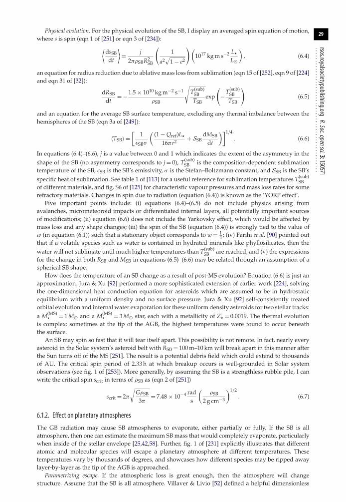
29


................................................Physical evolution. For the physical evolution of the SB, I display an averaged spin equation of motion,

where s is spin (eqn 1 of [251] or eqn 3 of [234]):⟨dsSB

dt

⟩= j

2πρSBR2SB

(1

a2√

1 − e2

)(1017 kg m s−2 L�

L�

), (6.4)

an equation for radius reduction due to ablative mass loss from sublimation (eqn 15 of [252], eqn 9 of [224]and eqn 31 of [32]):

dRSB

dt= −1.5 × 1010 kg m−2 s−1

ρSB

√T(sub)

SBTSB

exp

(−T(sub)

SBTSB

)(6.5)

and an equation for the average SB surface temperature, excluding any thermal imbalance between thehemispheres of the SB (eqn 3a of [249]):

〈TSB〉 =[

1εSBσ

((1 − Qref)L�

16πr2 + SSBdMSB

dt

)]1/4. (6.6)

In equations (6.4)–(6.6), j is a value between 0 and 1 which indicates the extent of the asymmetry in theshape of the SB (no asymmetry corresponds to j = 0), T(sub)

SB is the composition-dependent sublimationtemperature of the SB, εSB is the SB’s emissivity, σ is the Stefan–Boltzmann constant, and SSB is the SB’sspecific heat of sublimation. See table 1 of [113] for a useful reference for sublimation temperatures T(sub)

SBof different materials, and fig. S6 of [125] for characteristic vapour pressures and mass loss rates for somerefractory materials. Changes in spin due to radiation (equation (6.4)) is known as the ‘YORP effect’.

Five important points include: (i) equations (6.4)–(6.5) do not include physics arising fromavalanches, micrometeoroid impacts or differentiated internal layers, all potentially important sourcesof modifications; (ii) equation (6.6) does not include the Yarkovsky effect, which would be affected bymass loss and any shape changes; (iii) the spin of the SB (equation (6.4)) is strongly tied to the value ofw (in equation (6.1)) such that a stationary object corresponds to w = 1

4 ; (iv) Farihi et al. [90] pointed outthat if a volatile species such as water is contained in hydrated minerals like phyllosilicates, then thewater will not sublimate until much higher temperatures than T(sub)

SB are reached; and (v) the expressionsfor the change in both RSB and MSB in equations (6.5)–(6.6) may be related through an assumption of aspherical SB shape.

How does the temperature of an SB change as a result of post-MS evolution? Equation (6.6) is just anapproximation. Jura & Xu [92] performed a more sophisticated extension of earlier work [224], solvingthe one-dimensional heat conduction equation for asteroids which are assumed to be in hydrostaticequilibrium with a uniform density and no surface pressure. Jura & Xu [92] self-consistently treatedorbital evolution and internal water evaporation for these uniform density asteroids for two stellar tracks:a M(MS)

� = 1 M� and a M(MS)� = 3 M� star, each with a metallicity of Z� = 0.0019. The thermal evolution

is complex: sometimes at the tip of the AGB, the highest temperatures were found to occur beneaththe surface.

An SB may spin so fast that it will tear itself apart. This possibility is not remote. In fact, nearly everyasteroid in the Solar system’s asteroid belt with RSB = 100 m–10 km will break apart in this manner afterthe Sun turns off of the MS [251]. The result is a potential debris field which could extend to thousandsof AU. The critical spin period of 2.33 h at which breakup occurs is well-grounded in Solar systemobservations (see fig. 1 of [253]). More generally, by assuming the SB is a strengthless rubble pile, I canwrite the critical spin scrit in terms of ρSB as (eqn 2 of [251])

scrit = 2π

√GρSB

3π= 7.48 × 10−4 rad

s

(ρSB

2 g cm−3

)1/2. (6.7)

6.1.2. Effect on planetary atmospheres

The GB radiation may cause SB atmospheres to evaporate, either partially or fully. If the SB is allatmosphere, then one can estimate the maximum SB mass that would completely evaporate, particularlywhen inside of the stellar envelope [25,42,58]. Further, fig. 1 of [231] explicitly illustrates that differentatomic and molecular species will escape a planetary atmosphere at different temperatures. Thesetemperatures vary by thousands of degrees, and showcases how different species may be ripped awaylayer-by-layer as the tip of the AGB is approached.

Parametrizing escape. If the atmospheric loss is great enough, then the atmosphere will changestructure. Assume that the SB is all atmosphere. Villaver & Livio [52] defined a helpful dimensionless

30


................................................quantity

Γ ≡ GMSBMH

kBRSBTex, (6.8)

where Tex is the temperature of the exosphere (which may be different from the SB’s effectivetemperature), MH is the mass of a hydrogen atom and kB is the Boltzmann constant. The quantity Γ

represents the ratio of the gravitational potential energy to the particle kinetic energy, or the square ofthe ratio of the atmospheric escape velocity to thermal velocity. Villaver & Livio [52] found that theatmospheric structure is maintained for Γ � 20.

Determining Tex depends on how one models heat transfer within an SB atmosphere. This transfer isdetermined by a combination of convection and conduction. Villaver & Livio [52] neglected convectionbecause SBs orbiting GB stars are unlikely to be tidally synchronized. Consequently, they solved aconduction-dominated energy equation (their eqns 6 and 8) in order to obtain an expression whichcan be implicitly solved for Tex (their eqn 7) given a wide variety of thermal properties (conductivity,thermospheric base temperature, intensity reaching atmosphere).

Quantifying escape—number density flux If the atmospheric structure is maintained (Γ � 20), then alower limit to the escape rate by thermal evaporation can be expressed through a number flux Φ as(eqn 9 of [52])

Φ = −√

kBTex

2πMHδ(1 + Γ ) exp(−Γ ), (6.9)

where δ is the number density of the escaping constituent. The restriction that Γ � 20 limits the useof equation (6.9). A more complete treatment requires considering potential feedback factors, rampressure stripping, photodissociation, immersion into a postshocked hot bubble, and the solution ofthe atmospheric structure equations; estimating the result with a single explicit expression like theireqn 10 still requires many assumptions that rely on results of numerical simulations anyway. Also, assuggested by Spiegel & Madhusudhan [131], extant pebbles and boulders could be accreted onto theSB’s atmosphere during post-MS evolution due to N-body interactions (see §7), altering the compositionand structure of the atmosphere.

Quantifying escape—mass flux. With the same functional form of equation (6.9), Livio & Soker [248]provided an expression (in their eqn 6) for SB atmospheric mass loss while in the midst of a redgiant. More recent treatments have also been provided [43,129]. Bear & Soker [43] incorporated bothevaporation and ionization of the evaporated gas, and pointed out that recombination of the ionizedgas is not necessarily an important process for MS exosystems, unlike in post-MS exosystems. Bymanipulating and rewriting their eqns 7 and 10, as well as assigning a negative sign for mass loss, Iobtain

dMSB

dt≈ −1

2

⎡⎣2πGMSBv2

outηΠR +

√4π2G2M2

SBv4out

η2Π2R2 + 8πRSBv2outHEUV

ΠR

⎤⎦ , (6.10)

where vout is the outflow speed, η is the efficiency factor for channeling EUV radiation to evaporation,Π is the average energy of ionizing photons, R is a recombination rate coefficient and HEUV is the totalEUV power from a given wavelength range. Some characteristic values might be vout = 2 × 105 m s−1,η = 0.2, Π = 20 eV, R= 5 × 1034 m3 kg−2 s−1 and HEUV = 4 × 1023 J s−1.

Giant planet atmospheres—chemical changes. Campbell et al. [52] and Spiegel & Madhusudhan [131]are important studies because they speak directly to the fate of the giant planets in our Solar systemand, in particular, Jupiter. We know that Jupiter will survive Solar mass loss and not undergo scatteringinstability, but will it evaporate completely? Section 4 of [131] is devoted to the chemical changes Jupiterwill undergo during the Sun’s post-MS evolution, as well as what Jupiter’s spectrum would look like(their fig. 6). This spectrum includes some abundance alterations in carbon, methane and water.

6.2. Compact object radiation

6.2.1. White dwarf radiation

Comet sublimation WD radiation causes an SB to lose mass, particularly if the SB is volatile rich. This massloss may arise in the form of sublimation or outgassing. Veras et al. [254] made a distinction between thetwo terms, referring to the former as the homogeneous mass exodus of surface particles and the latteras localized violent eruptions. In either case, from equations (4.3)–(4.9), one can see that whatever massis lost from the system by the SB will negligibly change its orbit. Instead, the largest orbital change will

31


................................................come from the kick due to mass loss-induced linear momentum recoil. Veras et al. [254] did not treat thekick as impulsive. They assumed the SB was continuously losing mass in a manner physically motivatedby Solar system comets.

By assuming that an SB has a volatile content M(vola)SB which is subject to sublimation and is made of

a single species with molecular or atomic mass Mvola, they found that the equations of motion become(their eqn 6)


r3 r − {H(M(vola)SB )} D0v0Mvola

MSB − M(vola)SB

( r0

r

)9/4 rr

, (6.11)

where H is the Heaviside function and D0, v0 and r0 are fiducial values representing, respectively, thenumber of molecules or atoms of the volatile species sublimating per time, the mean ejection velocity ofthat species, and distance to the WD.

Using this formulation, Veras et al. [254] found that for nearly parabolic orbits (e � 0.998)—as expectedof SBs which pollute WDs—the orbital pericentre robustly resists changes to sublimative forces eventhough other orbital parameters might easily change. They generalized this result to arbitrary integralpower-law dependencies on distance (their appendix A). Therefore, comets whose orbital pericentre isoutside of the WD disruption sphere will not self-perturb themselves into the disruption sphere unlessacted on by other agents.

Stone et al. [67], using a different set of assumptions than Veras et al. [254], approximated the location,rsub at which a volatile-rich SB completely sublimates. By generalizing eqn 12 of [67], I obtain

rsub ∼ 9L2�

64GM�R2SBρ2

SBT 2SB

, (6.12)

where TSB is the SB’s latent heat of transformation (given as 3 × 1010 erg s−1) and is claimed to be similarfor ice and silicates. If instead the comet partially sublimates at each pericentre passage, and the amountof mass lost per passage decreases steeply enough, then the total mass lost can be approximated by anconverging sum as in eqn C2 of [67].

Stone et al. [67] also, in their footnote #4, estimates the terminal speed of ice ejected to be

vterm =√

14kBTice

27MH, (6.13)

where kB is the Boltzmann constant, Tice is the sublimation temperature of ice and MH is the mass ofa hydrogen atom. They commented that the ejection velocity for dust is highly model-dependent (andhence more unconstrained than ice). They also discussed and quantified the potential distribution ofdebris left over from cometary sublimation (see their sections 3.2–3.3). These distributions rely on thespecific orbital energy of the sublimating debris.

Drag on substellar bodies. Besides mass loss, the pressure of WD radiation on SBs will cause them todrift inward according to equation (6.1). Belts or rings with non-uniform size distributions might thenrespond to WD radiation in complex ways. I discuss the implications of this process in the context offorming WD discs from first-generation SBs in §9.

Sublimating white dwarf debris discs. WD radiation plays a crucial role in the morphology andevolution of WD debris discs. This radiation sublimates dust into gas and mingles the two. I discussthe implications of this sublimation in §11.

Effects on substellar body atmospheres. The relatively small size and quickly dimming nature of WDsprovide for interesting SB atmospheric dynamics. In contrast with the extreme MS planet Kepler-91b,which is so close to its parent star that 70% of the planet atmosphere is illuminated by the host star (fig. 10of [10]), in WD systems much less than 50% of a giant planet atmosphere would be illuminated (theradius of a WD is an order of magnitude smaller than that of a giant planet). I summarize SB atmosphericstudies from WD systems in §12.4 in the context of climate and habitability.

6.2.2. Pulsar radiation

The radiation emitted from pulsars contains highly energetic and relativistic particles. The consequencesfor SBs are different than in MS, GB and WD planetary systems. Also, processes like ohmic dissipation, orinduction heating (see Appendix B of [194]), might not be as prevalent in MS, GB or WD systems. Further,pulsar radiation evaporates and ionizes infalling bodies. When remaining charges are accelerated torelativistic energies, they can interact with the magnetic field to produce observable signatures [193].

32


................................................Implications for second-generation formation. In the context of second-generation formation, relativistic

particles can break apart complex nuclei and prevent metals from forming [73]. Therefore, shieldingfrom particle radiation may be necessary to allow planet formation for a high-enough luminosity.Miller & Hamilton [73] considered how the luminosity of a pulsar changes as it is being spun-up, withimplications for second-generation planet formation (see §8).

Implications for formed substellar bodies. The putative asteroid disc that orbits PSR B1937+21 might becomposed of many asteroid-sized objects on non-crossing orbits that range down to a few tenths of anAU [186]. Consequently, the Yarkovsky effect, driven by the magnetosphere from beamed X-rays, mightplay a significant role in the evolution of this disc. They adopted the formalism of Cordes & Shannon[194] and find that only SBs with RSB � 5 km could survive infall due to the Yarkovsky effect if in thenascent disc a � 1 AU. This estimation provides a strong constraint on the potential present-day sizedistribution in the disc.

7. Multi-body interactionsThe forces I described in §§4–6 involve the star and SB only: effectively, the two-body problem. Now Iconsider the N-body problem, where N ≥ 3 and one of the bodies is the parent star. Because the three-body problem is generally unsolvable, N-body interactions—particularly in post-MS systems with somany additional forces involved—are often modelled with numerical simulations, a prominent themein this section. The actual computer codes used by the authors are not mentioned here, but rather in adedicated section (§14) for easier reference.

A single N-body numerical integration of a chaotic system is not a deterministic prediction. Fig. 1bof [255] illustrates the maximum eccentricity that the planet Mercury will achieve over the next 5 Gyr:this value can vary by nearly unity for two simulations with equivalent initial conditions except for avariation of 0.38 mm in Mercury’s initial semi-major axis. The authors refer to the search of a precisesolution over this interval as ‘hopeless’.

Although the long-term MS orbital evolution of planets and planetesimals has been studiedextensively (see [256] for a review), rarely have previous investigations carried out numericalintegrations for the entire duration of the MS. Consequently, the initial orbital architectures for post-MSstudies are poorly understood, much less the subsequent multi-body interactions with the complexitiesintroduced by GB evolution.

Common simulation features. A common assumption is that all SBs change their orbits simultaneouslydue to stellar mass loss. In reality, there is an ejecta-lag crossing time. The orbit of the closest SB will shiftbefore the orbits of any other SBs. The consequences of this assumption have not yet been explored indetail, but are likely to be greatest, as pointed out by Veras et al. [24], (i) for widely spaced orbits, and/or(ii) for non-adiabatic mass loss dynamics. According to observations [33], ejecta may take on the order of100 days to travel just 1 AU.

Also, simulations which feature mass loss do not conserve energy. Many, however, do conserveangular momentum. Angular momentum conservation then provides an important check on theaccuracy of simulations and a check on the physics. Bear et al. [41] demonstrated how conservationof angular momentum arguments alone can help exclude additional bodies from playing a significantdynamical role (or existing at all) during the history of a system.

In the common case of SBs experiencing adiabatic motion due to stellar mass loss, while the systemis stable, eccentricity variations can be attributed primarily to their mutual interactions rather than frommass loss. The true anomaly and eccentric anomaly evolution is also negligibly affected by mass loss.These attributes are useful for disentangling the effects of mutual interactions and mass loss.

7.1. Collisions within debris discsGiven the variety of forces affecting substellar bodies in post-MS systems, debris discs may geometricallyrepresent ‘discs’ only in a loose sense. Nevertheless, for the purposes of this section, assume that the disccan be represented by an annulus with inner and outer boundaries represented by r(min)

d and r(max)d , where

r is exactly in-between those two values.If mutual velocities are sufficiently high for collisions to be destructive, then collisional erosion

continuously replenishes smallest bodies. Therefore, the collisional lifetimes of bodies of different sizesare key parameters. In general, the collisional lifetime, tcoll, for particles of a given size is provided by

33


................................................

0 100 200 300time in Myr since start of GB phase

disc

mas

s in

M

�

10 AU

50 AU

100 AU

102

1

10–2

10–4

1 M�

10 M�

100 M�

400 500 600

Figure 10. Cosmetically enhanced version of the lowest panel of fig. 4 of [32]. How GB evolution of a M(MS)� = 2.9M� star depletes

a debris disc due to collisional evolution alone. The legend indicates the initial disc masses. The solid lines correspond to {r = 10 AU,r(min)d = 7.5 AU, r(max)d = 12.5 AU}, the dotted lines correspond to {r = 50 AU, r(min)d = 37.5 AU, r(max)d = 62.5 AU} and the dashed linescorrespond to {r = 100 AU, r(min)d = 75 AU, r(max)d = 125 AU}.

eqn 7 of [257] as

tcoll = 2〈i〉r5/2(r(max)d − r(min)

d )√

GM1/2� Σdξb

(7.1)

with Σd representing the cross-sectional area, ξ representing the ratio of the relative collisional velocityto the Keplerian velocity and b representing the fraction of the disc’s cross-sectional area in whichcatastrophic collisions with these large objects may occur. Generally, tcoll decreases as the disc approachesthe central star. The shorter the collisional lifetime, the more quickly collisional equilibrium is reached.In this case, memory of the initial mass is erased. However, collisional equilibrium might not hold for allevolved discs [258].

Various specific cases of equation (7.1) have been used in the subsequent literature. Among the mostrelevant for post-MS evolution is contained within the study by Bonsor & Wyatt [32]. They find that thedisc mass evolves according to (their eqns 20 and 21)

M(GB)d = M(MS)

d

[1 + CM(MS)

d

∫M17/3

� dt]−1

, (7.2)

where

C ≡[

2.8 × 10−9

(r(max)

d − r(min)d

r

)e−5/3 max(RSB)Q5/6r(MS)13/3

M(MS)�

13/3]−1

(7.3)

and Q is the dispersal threshold for collisions. Figure 10 illustrates how disc mass decreases with timeaccording to equation (7.2).

7.2. One star, one planet and asteroidsAt least five investigations so far [59,61,227,259,260] have modelled the post-MS interactions betweenone planet and a collection or sometimes belt of smaller objects with numerical simulations.

7.2.1. A Kuiper belt with a Neptune

Bonsor et al. [259] modelled a 1 M� MS star that loses 23 of its mass at a constant rate (6.7 × 10−6 M� yr−1)

over 105 yr. Because of the constant mass loss rate assumption, stellar metallicity is not taken intoaccount. They placed a Neptune-mass planet initially at 30 AU in a circular orbit, with 500 test particleswith initial semi-major axes from 30 to 47.6 AU such that their initial eccentricities and inclinations wereless than 0.1 and 10 degrees, respectively. In effect, this setup represents a cold exo-Kuiper belt. Giventhe distances involved, stellar mass loss is adiabatic in all their systems.

In order to develop initial conditions for the post-MS simulations, they integrated these systems for107 years with a static parent star (along the MS) to scatter away dynamically fragile members and settle

34


................................................1.00

0.1

0.2

tidally disruptedasteroid

0.3

1.5 2.0orbital period of planet/orbital period of asteroid

ecce

ntri

city

of

aste

roid

2.5 3.0

Figure 11. Cosmetically enhanced version of fig. 2 of [59]. How the GB-induced expansion of the libration width of the 2 : 1 meanmotionresonance between a planet and asteroids induces the latter to be scattered towards and inside of the WD disruption radius. The solidand dashed lines are the libration widths for, respectively,M(MS)

� = 1.0M� andM(WD)� = 0.5M�. Note that a couple asteroids near the

3 : 2 mean motion commensurability are also scattered towards the WD and disrupted.

the belt. This timescale is typically three orders of magnitude smaller than MS lifetimes, and was adoptedto effectively create a largely dynamically settled exo-Kuiper belt.

The simulations demonstrate that changing stability boundaries from mass loss allow a fraction of thebelt to be scattered inwards, creating an inner reservoir of material after the star has become a WD. Ifadditional planets on circular orbits exist inward of the Neptune, then subsequent scattering with the testparticles can be constrained analytically, and allow these particles to achieve WD-grazing orbits [261].

7.2.2. An asteroid belt with a Jupiter

Debes et al. [59] simulated the orbital evolution of one planet with the physical and orbital propertiesof Jupiter, along with 710 interior-lying asteroids with orbital properties equivalent to Solar systemasteroids. The parent star contained 1 M� on the MS, and lost 0.46 M� over 1000 years accordingto a prescription from Schröder & Smith [230], corresponding to an average mass loss rate of 4.6 ×10−4 M� yr−1. Ten simulations were run for 100 Myr, four for 200 Myr and three for 1 Gyr. Theirsimulations tracked test particles until they reached 1R�, upon which they were removed.

Debes et al. [59] also emphasized the importance of resonant interactions between a planet and testparticle. They showed how the libration width of the interior 2 : 1 mean motion resonance grows duringmass loss, capturing test particles (figure 11). The eccentricity of these particles then increase until theypotentially enter the WD disruption distance. Over all their simulations, about 2% of test particlesfollowed this path; just one asteroid per simulation disrupted after 200 Myr. They found that in order tomatch WD observations on aggregate, exo-asteroid belts would need to be between 4 × 100 and 6 × 105

as massive as the Solar system asteroid belt. The large range perhaps emphasizes that a single model hasdifficulty explaining the entire population of polluted WDs.

Frewen & Hansen [61] explored a wider region of phase space than Debes et al. [59] through a seriesof separate MS, GB and WD numerical simulations. The MS simulations were run for 0.1 Gyr (abouttwo orders of magnitude less than a typical MS lifetime), the GB simulations were run for 2700 yr andthe WD simulations were run for 1.0 Gyr. Among these simulations the authors adopted planet masses of0.03, 0.3, 1.0 and 4.0MJup and eccentricities of 0.02, 0.2, 0.4, 0.6 and 0.8 (one planet per simulation). In everycase, the planet’s MS and resulting WD semi-major axes were 4 and 7.42 AU, as the 1.0 M� MS parentstar was modelled to lose a total of 0.461 M�, and at a constant (1.7 × 10−4 M� yr−1) rate. The particlebelt surrounded the planet in order to achieve coverage of many first- and second-order internal andexternal mean motion commensurability locations. They discussed the potential importance of the effects

35


................................................of wind drag and Yarkovsky forces (their section 5.1), but did not include them in simulations. Thesesimulations importantly demonstrated that higher planetary eccentricities and smaller masses enhancethe accretion rate.

7.2.3. Other configurations

Dong et al. [227] performed a set of simulations with a single planet and a few planetesimals (see theirfigs 3–5). The planet mass was a Jupiter-mass, and the planet was initially placed on a circular orbit at20 AU. Planetesimals of different sizes were placed on circular orbits at 35 AU, and the 4 M� parent starwas made to lose mass linearly at a rate of 3 × 10−5 M� yr−1 for 105 yr. Unlike the above four studies[59,61,259,260], wind drag (see §4.3) was also included in the simulations from Dong et al. [227]. Theyillustrated that in this setup, capture into the external 3 : 2 mean motion resonance occurs.

7.3. One star, multiple planets and no asteroids

7.3.1. Few-planet stability boundary changes

Two planets. The discovery of the post-MS PSR B1257+12 planets in 1992 [1] provoked a resurgenceof interest in celestial mechanics and in particular the three-body problem. The following year,Gladman [262] conveyed a concept from algebraic topology—that of Hill stability (in a Hill stablesystem, two planetary orbits never cross)—to the wider astronomical audience by expressing the relevantcriterion in orbital elements and in the context of two coplanar small planets orbiting a star. A decadelater, Debes & Sigurdsson [211] then illustrated how in post-MS systems, mass loss can convert a Hillstable system into an unstable one. A decade after that, Veras et al. [24] considered this transition to Hillinstability with arbitrarily eccentric and inclined orbits. However, mounting progress in characterizinginstability in the few-body problem (see, e.g. [263] for a review) is not limited to Hill stability. Severalauthors have since popularized Lidov–Kozai motions, gave attention to Lagrange instability (a proxyfor the global stability boundary), and generally provided an appreciation for orbital architecturespreviously assumed to be unorthodox and perhaps ignorable (see [256] for a review).

Three planets. For systems with more than two planets, Hill stability no longer applies. Instead, authorshave introduced the concept of a critical separation for instability where a single relation links theconsecutive pairwise planet separations. Mustill et al. [264] derived the following estimate for the criticalseparation � (adapted from their eqns 2 and 6) assuming three equal-mass planets

� ≈ 0.7ainner

(MSB

3 M�

)1/3(

MSB

MJup

)−1/12 (M(i)

�

M�

)1/12 (M(f)

�

M(i)�

)−1/4

×[

logtf − ti

Myr− 1

2log

M(i)�

M�+ log

MSB

MJup− 3

2log

aAU

+ logM(f)

�

M(i)�

+ 11.0

], (7.4)

where the superscripts i and f refer to initial and final states, and not necessarily MS and WD. Thisrelation helps show that higher mass stars produce greater amounts of instability because the planet–starmass ratio becomes more unequal.

More than three planets. For more than three planets, Duncan & Lissauer [223] found a roughly linearrelationship between instability time and amount of stellar mass lost. Veras & Gänsicke [144] quantifiedthe initial separations for which the planetary system would significantly alter its initial configuration (orbecome unstable, by some definitions). They adopted the mutual separation distance formulation (seetheir eqn 1) from Smith & Lissauer [265], which is measured in number of ‘mutual Hill radii’, denotedby β. Veras & Gänsicke [144] found that closely packed giant planets with β ≈10–12 typically unpack orbecome unstable during the post-MS phases. For terrestrial planets, instead β ≈ 6.

7.3.2. GB and white dwarf planet simulations

Two planets. In 2002, Debes & Sigurdsson [211] demonstrated that adiabatic mass loss changes thestability boundary in multi-planet systems, and can induce instability in previously stable systems. Theyillustrated that although the ratio of semi-major axes of two planets remained unchanged through theGB phases, the critical Hill stability separation does not scale in the same way. Consequently, during GBmass loss, two planets can cross this boundary. They performed numerical simulations which involvedincreasing the mass of the planets rather than decreasing the mass of the star. The planet mass increase

36


................................................

1.15

WD

MS

10

8

6

4

2

1.25

log 10

(t in

st in

yr)

1.35

MS

Hill

sta

ble

limit

MS

lagr

ange

sta

ble

limit

WD

lagr

ange

sta

ble

limit

initial semi-major axis ratio of both planets1.45 1.55

5 : 4 4 : 3 3 : 2 5 : 3 2 : 1

Figure 12. Cosmetically enhanced version of the bottom-rightmost panel of fig. 9 of [24]. I show instability timescales, tinst, as blackdots for individual two-planet simulations with the given initial semi-major axis ratio and all with a parent star ofM(MS)

� = 3.0M�. Bluestars indicate that all simulations sampled at that particular semi-major axis ratio were stable over a total of 5 Gyr of evolution. The twocoloured horizontal lines represent the RGB and AGB phases, and the upper axis illustrates some mean motion commensurabilities. Thisplot demonstrates that (i) systems which are stable on the MSmay become unstable beyond the MS and (ii) that Lagrange instability onthe MS can manifest itself late, right before the RGB phase.

corresponded to a halving of the stellar mass over 105 orbits of the inner planet; the simulations wererun for up to 107 of these orbits. The authors adopted planet–star mass ratios of 10−7, 10−5 and 10−3.

The complementary work of Voyatzis et al. [215] a decade later explored how non-adiabatic mass losschanges stability in two-planet systems. For real systems with stars that become WDs, this situationwould arise only for two SBs which are at least several hundred AU away from the GB star. Theyfound that the resulting changes in eccentricity enhance the prospects for instability. One way of tracingthe susceptibility of a two-planet system to become unstable over a Hubble time (or current age ofthe Universe) is to track the Lyapunov exponent [200,215]. Adams et al. [200] found that althoughthe Lyapunov exponent varies by orders of magnitude depending on the mass loss timescale, bothtimescales are comparable.

Motivated by instability induced by crossing the Hill stable boundary, Veras et al. [24] performednumerical integrations incorporating both planetary and stellar evolution for two planets across allpost-formation phases of evolution. They adopted ainner = 10 AU, M(MS)

� = [3, 4, 5, 6, 7, 8]M�, and ransimulations for 5 Gyr, a long enough period to cover the MS and GB phases and several Gyr on theWD phase (see their fig. 7). They primarily adopted initially coplanar planets with Jovian masses,eccentricities of 0.1 and initial separations that cover a range of possible stability outcomes (see fig. 12 ofthis paper).

Their results demonstrated that (i) post-MS mass loss alone can trigger instability not only during theGB phase, but well after. In fact, because in almost every case the mass loss is adiabatic, the architectureof the system inflates without a notable initial change. But that process in effect ‘resets’ the system, so thatsubsequent dynamical instability occurs on timescales similar to those one might expect after formationon the MS (figure 12). (ii) The ejection of one planet perturbs the other onto a moderately to highlyeccentric orbit, sometimes with an orbital pericentre of just a few AU. This eccentric planet could thenperturb any interior asteroids (not modelled), providing a dynamical environment for pollution. Due toconservation of angular momentum, the semi-major axis of the surviving planet is well-approximatedanalytically (see their eqn 8 and figs 14 and 16), unlike its eccentricity, which can be determined only ifthe hyperbolic eccentricity and semi-major axis of the escaping planet are known.

Three planets. In a follow-up paper that integrated systems with three Jovian planets instead of two,Mustill et al. [264] improved upon Veras et al. [24] in several respects, including: (i) they explored multi-generational instability. For example, with three planets, one instability can occur on the MS, with thesecond on the WD (see their fig. 5). In about 1% of all cases, all three planets were lost. (ii) Theymore accurately quantified the fraction of unstable post-MS systems which lead to direct planet–WDcollisions by adopting the WD disruption radius instead of the actual WD radius, and by giving thethree planets slightly non-coplanar inclinations (in line with Solar system observations). They foundthat, like in the two-planet case, ejection during the WD phase is the most commonly occurring type

37


................................................

0

100

10

1

0.1

10–2

1 2 3 4 5 6 7time in Gyr

orbi

tal p

eric

entr

e in

AU

detectableby

transit?

MS WD

M (t = 0) = 1.5 M�GB

breaksup

R ,GB(max)

8 9 10 11 12 13 14

Figure 13. Cosmetically enhanced version of the upper-left panel of fig. 1 of [144]. Late unpacking of four tightly-packed terrestrialplanets throughout theMS and GB phases. The orbit meandering which follows scattering instability perturbs the red planet into a likelytransit-detectable orbit before it enters the WD disruption radius.

of instability (see their fig. 4). These ejected planets help ensure that WD planets rarely evolve to a hotJupiter state, and provide a potentially non-negligible contribution [266] to the purported free-floatingplanet population [267].

More than three planets. Veras & Gänsicke [144] then extended earlier work [24,264] by adoptingM(MS)

� = 1.5 − 2.5 M�, which corresponds to the primary source of progenitors of the currently observedWDs (figure 3), and by considering the evolution of packed systems with four and ten planets. Theyalso integrated these systems for the current age of the Universe, 14 Gyr, and focused on lower-mass,terrestrial planets. As figure 13 demonstrates, these packed, stable and quiescent terrestrial planets on theMS can remain so throughout the GB phase, and for several Gyr along the WD phase, before ‘unpacking’.Subsequent to unpacking, the planets may meander and approach the WD closely enough for tidalcircularization to occur, increasing prospects for transit detectability by decreasing the orbital period.Interactions between these terrestrial planets were not strong enough to cause escape in any of theirsimulations, unlike for the giant planet case, representing a fundamental difference between their earlierstudies ([24] and [264]).

More than three planets plus moons. The presence of exo-moons in WD systems can provide a potentiallyimportant mass reservoir for heavy metal pollution. In our Solar system, the total mass of moons exceedsthat of the asteroid belt by over two orders of magnitude. Using the data from the simulations of Veras& Gänsicke [144], Payne et al. [268] considered how susceptible moons are to planet–planet scatteringwhich occurs during the WD phase. They found that after adiabatic mass loss, the Hill radius rHill of aplanet increases according to (their eqn 7):

r(WD)Hill

r(MS)Hill

=(

M(MS)�

M(WD)�

)4/3

. (7.5)

Nevertheless, even though moons become more entrenched, and hence stable, after post-MS mass loss,Payne et al. [268] showed that planet–planet scattering on the WD phase is highly destructive to moons.They demonstrated that moons may be regularly liberated from their parent planets. Although theultimate fate of the moons was not explicitly tracked, the moons may subsequently be perturbed intoWDs directly or act as agents to perturb smaller bodies, fragments or dust into WDs.

One earlier work [223] performed a variety of multi-planet simulations with different planet–starmass scalings which mirror those measured in the Solar system. In some cases they treated mass lossas constant, and in others used a fitted, observationally-motivated prescription. The latter case helpsdemonstrate that the four outer Solar system planets are likely to survive post-MS mass loss and remainstable at least for tens of Gyr (see §13).

7.3.3. Pulsar planet simulations

The exquisite data available for PSR B1257+12 [269] (with e.g. eccentricity accuracy at the 10−4 level)represents an opportunity to study the dynamics of a multi-planet system at a standard of detail that is

38


................................................largely unattainable in MS planetary systems. Gozdziewski et al. [270] performed an extensive analysisof the system with 1 Gyr numerical integrations, stability maps and Lyapunov exponent analyses. Theyfound (i) the system is long-term stable, (ii) none of the planets experience (notable) secular variations insemi-major axis, eccentricity or inclination, (iii) the outermost two planets are locked in a secular apsidalresonance with a libration centre of 180◦ and (iv) the line of nodes of the inner planet must be within 60degrees of the nodes of the outer planets.

7.4. Two stars, planets and no asteroidsSimulations for this physical setup cover a wide range of physical architectures and numerical codes.Here, I divide previous investigations according to whether or not the numerical codes adopted modelstellar evolution.

7.4.1. Simulations not incorporating stellar evolution

PSR B1620-26 The fascinating PSR B1620-26 system contains a millisecond pulsar (PSR B1620-26A), aWD (PSR B1620-26B) and a circumbinary planet (PSR B1620-26AB b) [135]. The dynamical pathwayleading to this scenario is thought to proceed along the following lines: (i) the planet forms around theMS progenitor of the currently-observed WD, (ii) that MS star-planet system flies by a NS and its originalunknown companion within the M4 globular cluster, (iii) this flyby induces an exchange reaction, wherethe NS’s companion is ejected and the NS captures the star and planet, (iv) the planet begins orbitingboth stars in a circumbinary fashion, (v) the MS star evolves into a GB star, (vi) mass transfer from theGB onto the NS spins the latter up and converts it into a millisecond pulsar and (vii) the GB star evolvesinto a WD. The result is the currently observed system.

The third part of this scenario was simulated with four-body dynamics [133], and remains an accuratequalitative description of the exchange despite the now-outdated orbital parameters used. This exchangeoccurs too quickly for stellar evolution to play a role.

Post-CE binaries. The future dynamical stability of the putative post-CE binary planetary systems (§3.4)have been explored with simulations in many studies: for HU Aquarii (HU Aqr) [271,272]; for QS Virginis(QS Vir) [273]; for NSVS 14256825 [274]; for NN Serpentis (NN Ser) [275]. The overall conclusions fromthese investigations is that all systems except for NN Ser undergo instability on short (approx. 103 − 104

years) timescales, placing doubt on the planetary interpretation of the signals. However, a few isolatedlong-term stable solutions also do exist for HU Aqr. Marsh et al. [175] criticized the above studies byclaiming that the initial conditions for their simulations are not consistent with the data, as the strongcorrelations between the orbital parameters were not taken into account. They do not necessarily believethat the qualitative stability conclusions of these other papers would change as a result, but do think thata re-evaluation is needed to be sure.

7.4.2. Simulations incorporating stellar evolution

The intriguing dynamics of post-MS evolution in binary systems which hosts planets has been exploredwith stellar evolution simulations by only a handful of investigations. The first two presented here[176,276] took alternate approaches to studying two of the post-CE binary systems from the last section:NN Ser and HU Aqu. The third [277] is an altogether different type of study that considered how a planetcan ‘hop’ from one star to another, and the fourth [278] quantified where circumbinary planets are subjectto escape.

NN Ser. For the purposes of investigating the stability of NN Ser, Mustill et al. [176] took an alternateapproach from Horner et al. [275] by looking at its past rather than its future. If the putative planetscould not maintain stable orbits on the MS, then the current observations are of either second-generationplanets, or of other phenomena entirely. Through the GB phases, the planets’ orbits increase due toadiabatic mass loss (see §4) while the stellar binary orbit shrinks because star–star tides dominate theevolution of their mutual orbit (see their fig. 1). Therefore, the MS stability of this system is moreprecarious than after the CE because a(MS)

inner < a(GB)inner, a(MS)

outer < a(GB)outer and a(MS)

b > a(GB)b .

To perform this investigation they (i) computed what MS orbital and physical parameters of the binarycorrespond with current observations by using a stellar evolution code, (ii) analytically determined,by assuming adiabatic mass loss and negligible other forces, the MS orbits of the putative planets and(iii), finally, integrated them along the MS with a planetary evolution code to assess their stability. Theyfound that in nearly all (99.74%) cases the planets become unstable before the end of the MS of the highermass star, suggesting that the currently observed planet candidates do not have a first-generation origin.

39


................................................HU Aqr. The putative planets around the cataclysmic variable HU Aqr are less certain to exist

because of the widespread instability found amongst the simulations performed [271,272]. Nevertheless,the existence of at least one long-term stable solution prompted Portegies Zwart [276] to perform a‘reconstruction’ of the dynamical history of that system through its CE phase.

As a first step, Portegies Zwart [276] determined what physical and orbital binary system parametersreproduce the system seen today. Then, he integrated the planets’ orbits by making assumptions aboutthe CE, such as the CE resulting in differing mass loss rates felt by both planets. An important outcomeof that study is the ability to restrict CE parameters, assuming that the planets exist now in the post-CE phase. He found that the fraction of orbital energy needed to unbind the CE during inspiral was45 ± 17%.

Planet hopping. Kratter & Perets [277] explored the exciting possibility that an SB can unbind from itsparent star due to stellar mass loss and then be captured by the stellar companion, performing a ‘hop’.This mechanism works because the change in the SB’s orbit is greater than the binary companion’s if theexpansion of both are adiabatic (a realistic possibility for ab � 103 AU). Suppose the binary companion isan MS star which remains as such throughout the primary star’s post-MS evolution. Suppose also thatthe primary star becomes a WD. Then, assuming full adiabaticity, MSB M�, and MSB Mb, I obtain(see also eqn 6 of [279])

a(WD)b = a(MS)

b

(M(MS)

� + Mb

M(WD)� + Mb

)(7.6)

and

a(WD)SB = a(MS)

SB

(M(MS)

�

M(WD)�

). (7.7)

The other orbital parameters remain the same in the adiabatic limit (see §4.1). The differential orbitalexpansion of the binary and planetary orbit in addition to the mass change can (i) allow a stabilitythreshold to be crossed, or, as explored by Bonsor & Veras [260], (ii) allow the binary orbit to be wideenough to incite future instability due to Galactic tides. If the binary orbital expansion in non-adiabatic,but the planetary expansion is adiabatic, then a previously stable system might remain so, depending onthe effect of Galactic tides.

As explained further by Kratter & Perets [277] and visualized in their fig. 2, in order for the SB to becaptured by the binary companion, the Jacobi constant must adhere to certain values. Although definedfor the circular restricted three-body problem with fixed masses (including one massless particle), theJacobi constant still represents a reliable proxy for capture in post-MS binaries with a single planet.

Kratter & Perets [277] performed simulations with 70 different binary configurations which includedifferent stellar masses, binary separations in the range a(MS)

b = 75 − 105 AU and a fixed a(MS)SB = 15 AU,

e(MS)b = 0.0 and e(MS)

SB = 0.0. They ran simulations for the entire duration of mass loss, plus 30 Myr. Theiroutputs show that about 10% of all SBs are captured by the companion, with typically prograde eccentricorbits satisfying e(MS)

SB > 0.4. Unstable systems typically featured a planet–star collision.Circumbinary escape Veras & Tout [278] instead determined where in phase space will a circumbinary

SB’s evolution become non-adiabatic (defined as Ψ > 1; see equation (4.10)) and consequently in dangerof escape due to post-MS evolution. They illustrated this critical SB semi-major axis in a series of contourplots, which explored dependencies on stellar masses (both M(MS)

� and M(MS)b ranging from 0.2 M�

to 8 M�), initial binary semi-major axis (ab = [10, 50, 100, 500, 1000, 5000]R�), initial binary eccentricity(eb = [0.0, 0.5, 0.9]), stellar metallicity (Z� = Zb = [0.0001, 0.0005, 0.001, 0.005, 0.01, 0.02]) and CE-blow offtimescale ([10, 102, 103, 104] years). The SBs themselves were not included in these stellar evolutionsimulations.

Veras & Tout [278] found that the complex physics of binary star evolution, which include CEs andSNs, reduces the adiabatic limit significantly (to several tens of AU) from the single-star case (at severalhundreds of AU). Therefore, the post-MS contribution to the free-floating exoplanet population [266]is expected to be higher for circumbinary rather than single star systems. Their study also backward-engineered the adiabaticity condition to yield a potentially useful constraint on stellar mass loss. Supposean SB is bound to two MS stars and harbours an initial semi-major axis a(MS)

CM with respect to the centreof mass of the stars. Now the primary star becomes a WD. During that process, the maximum value of|M�| which guarantees that the SB remains bound is (corrected from their eqn 6, which should contain

40


................................................an extra factor of G1/2; their eqn 4 is also missing a factor of G−1/2)

max(−M�) ≈√

G

⎡⎣ 1.4 M� + Mb√

a(MS)CM (M(MS)

� + Mb)

⎤⎦

3

. (7.8)

This result could be generalized to higher multiplicity cases or simplified to the single-star case (seetheir fig. 1).

7.5. Two stars, one planet and asteroidsBonsor & Veras [260] considered a set-up with an exo-Kuiper belt and a planet orbiting one star of a widestellar binary (rb ∼ 103 − 104 AU). After the parent star has become a WD the two stars experience a closeencounter due to Galactic tides (see §12.3 for more details). This encounter perturbs the planet, which isturn perturbs the asteroids into the WD, polluting it. They model a Neptune-mass planet on a circularorbit at 30 AU, and a belt of test particles from 30–50 AU. These simulations did not require the parentstar to evolve because it was already a WD. The dynamics of the encounter between the secondary star,planet and belt reveals that the more intrusive the encounter, the higher the rate of inwardly scatteredparticles.

7.6. Three stars onlyAlthough focused on the dynamics of hierarchical triple stellar systems with mass loss and without SBs,both Shappee & Thompson [62] and Michaely & Perets [280] derived results which may be applicableto SBs in the appropriate limits. Shappee & Thompson [62] modelled linear and adiabatic mass lossfrom a component of the inner binary with N-body integrations and considered the resulting change orinduction of Lidov–Kozai behaviour. Michaely & Perets [280] instead adopted a Hamiltonian formalism,derived doubly averaged equations including mass loss up to octupole order and derived the secularequations of motion in the case when all mass loss is adiabatic. They also consider the general case whenall three bodies lose mass. Secular equations allow for relatively quick integrations over long timescales,but by definition cannot resolve characteristics on orbital timescales.

8. Formation from stellar fallbackSome mass ejected by post-MS stars might not escape the system, and infalling material may bedecelerated due to phenomena such as reverse shock waves [281]. Both WDs and NSs could host remnantdiscs of matter through which ‘second-generation’ SBs form. First-generation SB formation proceedsat timescales less than 10 Myr. If second-generation formation is similar, then we should not expectit to occur later than WD or NS cooling ages of 10 Myr. Consequently, because the vast majority ofobservations of remnant planetary systems (§3.1) are snapshots in time where tcool 10 Myr, we arecurrently not observing activity from stellar fallback. Further, the chemical imprint of pollution observedwithin WD atmospheres is incongruous with the chemical composition of stellar mass ejecta.

Nevertheless, the prospect of second-generation formation of SBs at very early WD and NS coolingages remains viable, and has been explored by researchers for decades. The PSR B1257+12 systemwas a strong driver for this research [282,283], and recent pulsar observations [186,193] provide furthermotivation. Incentive also arises from putative planetary systems whose first-generation provenance isdisputed based on dynamical grounds (as in [25,176]). In an exceptional system like NN Ser, where theWD is known to harbour tcool ∼ 1 Myr [136], a second-generation planet would be the youngest knownexoplanet, and help constrain the formation process.

Second-generation formation provides intriguing possibilities for planetary system evolution.Perets [279] highlighted some important concepts on this topic: (i) post-MS evolution opens updynamically ‘previously forbidden’ regions of SB formation, (ii) pre-existing first-generation planetsmay interact with newly-formed second-generation planets, (iii) when each of two binary componentsundergoes post-MS evolution, there exists the prospects for third-generation formation, which is distinctfrom second-generation formation and (iv) second- and third-generation discs may be metal-enriched inorder to mirror the expected composition in stellar ejecta. These systems may conspicuously stand outin very metal-poor environments like globular clusters (on their outskirts, from dynamical stability) orsimply around metal-poor stars.

41


................................................8.1. Post-common envelope formation around white dwarfsThe amount of disc mass available for planet formation is a fraction of the amount of mass that remainsbound after the CE. The process for planet formation then proceeds along similar lines to the MS case,except here the disc may be influenced by photoheating, photoionization and radiation pressure (seesections 4.1–4.3 of [77]) in different manners. The metal content may also be different.

Bear & Soker [284] used angular momentum arguments to suggest that planets orbiting post-CEbinaries are more likely to be first generation than second generation. Their table 1 displays the minimumangular momentum of the putative post-CE binary planetary systems, as well as angular momentumefficiency factors for each system. The crucial unknowns are the efficiency factors, which determine(i) how much initial angular momentum is deposited into planets and (ii) how much of the envelopeends up in the disc. For NN Ser in particular, Schleicher & Dreizler [77] provided in their table 1 somemodel parameters for the formation by gravitational instability. Völschow et al. [220] observed that assecond-generation planets form in systems like NN Ser, the formation disc may still be expanding.

In WD–AGB binary systems, the formation of a second-generation disc may be quantified in a similarway as in an MS–AGB binary system. Through angular momentum arguments, Perets & Kenyon [285]provided a criterion for second-generation disc formation around the primary star from the wind of abinary companion (their eqn 1):

1 �(

M� + Mb

2.5 M�

)(M�

M�

)3/2 ( R�

R�

)−1/2 ( a100 AU

)−3/2(

|v(wind)b − v|

10 km s−1

)−4

. (8.1)

8.2. Post-supernova formation around neutron starsGeneral considerations Miller & Hamilton [73] and Hansen [286], and references therein, summarizedmultiple possible scenarios for the formation of a circumpulsar disc: (i) a disc forms from binary masstransfer, where the donor is disrupted or evaporated, (ii) a disc forms from donor ejecta, then the donor isevaporated, (iii) a disc forms from donor ejecta, and then the donor goes SN and gravitationally unbindsthe disc-bearing pulsar, (iv) a disc forms from ejecta from an SN-induced direct collision (where theSN kick was in the direction of the other star) and (v) a disc forms from ejecta from a WD–WD directcollision, which could form a pulsar and an accompanying disc. Second-generation pulsar planets donot necessarily need a disc if the planets either formed directly from fallback matter or the companionwas evaporated just the right amount to achieve a planet mass.

Miller & Hamilton [73], who do not favour first-generation scenarios for the known pulsar planets,also placed restrictions on post-SN second-generation formation through stellar evolution arguments:if a pulsar was transformed into a millisecond pulsar by accreting matter, then they argue that theluminosity from the accretion would evaporate the planet. If this accretion process occurred and lefta remnant second-generation disc, then the authors argued that stellar luminosity would disperse thedisc too quickly too allow for formation.

In a wide-ranging dynamical study of second-generation formation and evolution, the cleverly titledpaper by Cordes and Shannon [194] covered collisional migration, the Yarkovsky effect, magnetosphericcurrents, electromagnetic capture, heating and evaporation of SBs, and disc lifetimes. Their main findingis that second-generation asteroids, but not planets, could easily form and create observable signaturesin systems like B1931+24. This scenario relies on (i) the SN fallback disc to be metal-rich and ‘sufficientlycompact and low in mass (10−6 M�) to prevent’ massive planet formation, (ii) the mass inflow intothe light cylinder to be large enough to influence magnetospheric current flows on relevant timescalesand (iii) the disc survival time must be long enough (greater than or equal to 10 Myr) to alter theelectrodynamics of old pulsars. A couple of interesting ancillary findings include the fact that (i) rockswith high tensile strengths can form metal-rich gas inside the tidal disruption radius. These second-generation rocks are not like the strengthless rubble piles seen in the Solar system because they aremetal-rich and fractionated. Further, (ii) the radiative effects on second-generation asteroids near thepulsar’s light cone are comparable to currently observed Solar system Yarkovsky drift rates (approx.10−3 AU Myr−1).

PSR B1257+12. Before delving into the possibilities for second-generation formation in PSR B1257+12,one may ask if mass loss alone hypothetically (ignoring engulfment) could induce ejection of the SBs. Tohelp answer this question, Veras et al. [208] considered the likely value of Ψ (see equation (4.10)) for thePSR B1257+12 planets during their SN mass loss. Even though the mass is lost from SN quickly, the smallMS semi-major axis values (<0.1 AU) of all three planets was too small to place them in the strongly

42


................................................non-adiabatic regime. Actually, Ψ ∼ 0.1–1.0, and therefore the planet eccentricities were not pumpedsufficiently high to cause ejection.

For a second-generation origin, Currie & Hansen [287] performed a dedicated modelling suite for thePSR B1257+12 disc. They considered both fully viscous discs and layered accretion discs. They found thatdiscs typically contain material out to 1–2 AU, and are sufficiently massive to produce the PSR B1257+12planets. Because the gas in these discs dissipates in under 0.1 Myr, gas giants are unlikely to form. Thefollow-up study of Hansen et al. [288] considered how planetesimals from second-generation discs wouldassemble into a planetary architecture. They found that because the density of solid material must besufficiently high for planet formation to commence, one can impose restrictions on the speed of dustsedimentation during disc cooling. Their study provides further support of the post-SN fallback scenario(as opposed to a binary companion disruption scenario) for the origin of the PSR B1257+12 planets.

8.3. Formation from tidal disruption of companionsPulsar stellar binaries. The PSR B1257+12 planets may have been formed through one of a few differentsecond-generation channels. Currie & Hansen [287] provided a comparison. Instead of forming outof stellar fallback, these planets might have formed out of shorn-off binary star matter. As opposedto fallback discs, with angular momentum values as low as 1042 J s−1, disruption discs could harbourangular momentum values three orders of magnitude higher. Because fallback discs tend to be morecompact than disruption discs, a fallback disc is more likely to reproduce the planets in the PSR B1257+12system. Similar to the SN fallback disc, in an SN disc formed from tidal disruption gas dissipates tooquickly to form giant planets.

In a similar vein, Shannon et al. [186] suggested that if the putative asteroid disc around PSR B1937+21is a second-generation disc, then it might have formed from the ablated material of a disrupted stellarcompanion. They proposed that the resulting disc was too tenuous to form planets, which is why noneare detected. Instead, the planet formation process would stop after a brief period of runaway growth,when asteroids were formed. Formation could occur throughout a radial distance of several AU, becausethe disc would not be truncated by the presence of planets. This second-generation disc itself mightfeature many SBs on non-crossing orbits and whose evolution is described in their sections 4.1–4.2.They suggested that inwardly-migrating SBs will never reach the star’s magnetosphere before beingevaporated.

White dwarf stellar binaries. Livio et al. [57] predicted the existence of second-generation debris discs,and possibly planets, around massive WDs as a result of a previous WD–WD merger. They envisagedthe merger of two 0.5 M� WDs forming a single approximately 1.0 M� WD with a residual disc. Basedon angular momentum arguments and a power-law surface density disc profile, they found

Md = 0.81 M�

(R�

r(max)d

)1/2

, (8.2)

where the inner (minimum) disc radius is presumed to coincide with the WD surface. They do not modelplanetesimal formation, but assume that it commences when r(max)

d exceeds the dust grain condensationline, which they estimated to be

r(dgline)d = 0.02 AU

(R�

6 × 106 m

)(T�

50000 K

)2⎛⎝T(dgline)

d1600 K

⎞⎠

−2

, (8.3)

where T(dgline)d is the disc temperature at which dust grains condense.

Large substellar bodies. Bear & Soker [289] indicated that while the envelope of a massive planet thatis being destroyed may form a gaseous disc, the rocky fragments could represent small planets thatthen migrate within the disc; Bear & Soker [290] made a similar suggestion. Alternatively, Guillochonet al. [291] and Liu et al. [292] intimated that a first-generation planet may be transformed into a second-generation planet by being tidally disrupted. In other words, after each close disruptive pericentrepassage of a gas giant planet and an MS (or, nearly equivalently, WD) star, the planet fundamentallychanges character. For coreless planets [291], when free-falling ejecta accretes onto the post-encounterplanetary remnant, then its outer layers spin faster and contain more mass, changing the atmosphericstructure. Although subsequent passages may destroy the planet, other bodies further away couldperturb the disrupting planet into a stable orbit. Cored giant planets can transform into super-Earthsor Neptune-like planets through this process [292].

43


................................................9. White dwarf disc formation from first-generation substellar bodiesThe compact debris discs which have been observed to orbit isolated (single) WDs at distances of(rd � 1.2R�) cannot have formed during the MS or GB phases. These discs also cannot have formedfrom fallback stellar material because of their age and composition. The canonical explanation is thatthey formed from the disruption of first-generation SBs [114,224,293], and in particular, asteroids. SeeFarihi [18] for an observationally based review of these discs. The orbits of the progenitors are assumedto be highly eccentric (e � 0.998) because their semi-major axes must be at the very least a few AU.Otherwise, these SBs would have been engulfed, vapourized or spun-up to fission during the GB phases.

Tidal disruption radius. Consequently, and emphasized by the WD 1145+017 system (see §3.2.1), theprocess of tidal disruption plays a crucial role in the interpretation of observations of post-MS systems.A primary consideration is then identifying the tidal disruption distance, rt, which defines a disruptionsphere, or Roche sphere, around the WD. This value depends on many factors, including the SB’s shape,spin state, composition and orbital state, as well as if disruption is defined as cracking, deforming ordissociating entirely.

A formulation which includes the internal strength of the SB is (rearranged from eqn 8 of [290]):

rt =[

2GM�ρSBR2SB

γSB + 43 πGρ2

SBR2SB

]1/3

, (9.1)

where γSB is the critical tensile strength of the SB that is disrupting. For a strengthless SB,which is representative of many ‘rubble pile’ Solar system asteroids, this equation reduces tort ≈ 1.26R�(ρ�/ρSB)1/3. However, because of the multiple dependencies mentioned above, Bear &Soker [294] re-expressed this relation in their eqn 1 with the following range of coefficients: rt ≈[1.3 − 2.9]R�(ρ�/ρSB)1/3. Alternatively, for bodies with high tensile strengths, equation (9.1) reduces toeqn 3 of [194], modulo a factor of 1.26. Another alternative is eqn 5 of [67], where the internal strengthdominates and the SB is characterized by solid-state forces and a corresponding internal sound speed.Then, rt ∝ G1/3M1/3

� R2/3SB v

−2/3sound. Typical SB speeds within the disruption radius can reach 103 km/s (eqn 7

of [295]).Tidal disruption simulations. The above relations allow one to consider modelling the process of tidal

disruption with analytics and simulations. Debes et al. [59] performed simulations of the breakup ofstrengthless 5000-particle rubble-pile asteroids by a 0.5 M� WD with initial orbital semi-major axes of4.77 AU and pericentres of 60, 65, 70, 75 and 80 R� (so e > 0.999). They modelled a single pericentrepassage and analysed the cumulative size distribution of the resulting fragments in the stream (see theirfig. 6). They found that for smaller pericentres, more large fragments are generated, and that the streamlargely followed the initial orbit.

Veras et al. [295] later also modelled the tidal disruption of highly eccentric strengthless 5000-particlerubble-pile asteroids, but did so for over 100 orbits. They established that the time an SB spends withinthe disruption sphere is largely independent of a (their fig. 1), enabling them to perform multi-orbitsimulations by scaling down the orbit. They found that the SB disruption eventually creates a highlycollisionless eccentric ring in the same shape as the original orbit, in the absence of other forces. Otherforces might cause the ring to become collisional, as suggested by Bear & Soker [294].

Ring formation analytics. Veras et al. [295] also derived a closed-form expression for the filling time, tfill,of this ring (their eqn 25) supposing that the breakup occurs instantaneously at some ru < rt:

tfill

PSB= r3/2

u

⎡⎣{ r2

u + 2aRSB − ruRSB

ru − RSB

}3/2

−{

r2u − 2amin(rcrit − ru, RSB) + rumin(rcrit − ru, RSB)

ru + min(rcrit − ru, RSB)

}3/2⎤⎦

−1

,

(9.2)

where PSB is the orbital period of the SB and where rcrit is the location at which the SB’s orbit wouldbecome parabolic

rcrit = 2aru(1 + MSB

M�

)(2a − ru)

≈ 2aru

2a − ru. (9.3)

Equation (9.2) does not make any assumptions about orbital eccentricity.However, as indicated by figure 2, considering gravity alone in a regime where r � 10−3 AU is

inadequate. Veras et al. [70] modelled the long-term effect of WD radiation on these collisionless rings.They found that WD radiation alone compresses and circularizes orbits of SBs with RSB ≈ 10−5–10−1 m towithin the WD disruption radius. See their eqns 20–22 for closed-form approximations of the evolution

44


................................................

10–2 10–1 1white dwarf age (cooling time) in Myr

orbital compression timescales

observeddiscs

au = 1000 AUau = 100 AUau = 30 AUau = 10 AUau = 5 AU

RSB = 10–5 m

RSB = 10–1 m

au = 1 AU

t shr i

n yr

t shr i

n yr

1

102

104

106

108

1

102

104

106

1010

108

10–2

1

102

104

106

108

1

102

104

106

1010

108

10–2

10 102 103 10410–3

Figure 14. Cosmetically enhanced version of fig. 2 of [70]. How particles of given radii and semi-major axis shrink due to the effects ofradiation alone, as a function of WD cooling time.

of a and e. Outside of this SB size range, radiative effects such as the Yarkovsky effect and radiationscattering may dictate the motion, and have not yet been explored. For this size range, they derive intheir eqn 23 a closed-form expression for the shrinking time tshr, which is better expressed as(

1 + 10(tshr + tu)Myr

)−1/5=(

1 + 10tu

Myr

)

− 2.39

(ρSBRSBc2q3/2

u

L�(tcool = 0)[Qabs + Qref]Myr

)(√au −√2qu + rt

), (9.4)

where c is the speed of light, where Qabs and Qref are the SB’s absorption efficiency and reflectingefficiency (albedo), tu is the cooling age at which disruption occurred, and au and qu are the orbital semi-major axis and pericentre at disruption. The value of tshr may change when additional effects, such assublimation, are taken into account. Figure 14 illustrates the shrinking time as a function of cooling age.Because the shrinking timescale is dependent on RSB, differently-sized pebbles will shrink at differentrates, fanning out the original ring. Further, as the SBs approach the WD, the effect of general relativitybecomes more important (see §12.1). Throughout the contraction, collisions may occur, which could affectsubsequent shrinking times.

Stone et al. [67] instead adopted a constant WD luminosity and in the high-eccentricity limit obtaineda characteristic shrinking timescale (their eqn D6) that is proportional to a1/2

u q3/2u /L�. The quality of this

approximation increases as the WD gets older, when L� experiences less-drastic changes.Other disruption processes. How the tidal disruption of an asteroid encountering a WD compares with

much better-studied tidal disruption situations in the literature is not yet clear. As observed by Bear &Soker [294], stars that pass close to black holes typically result in about half of their mass being ejected,with the remaining mass residing on highly eccentric orbits. A perhaps more relevant case are planetsdisrupting around MS stars [291,292]. In a rough qualitative sense, this situation should be similar forplanet destruction around WDs.

10. White dwarf disc evolutionOur understanding of how WD discs evolve crucially impacts observational targeting strategies andtouches upon both how these discs formed (§9) and how they accrete onto the WD (§11). More directlyand perhaps just as importantly, we cannot yet explain the variability in the dusty components of discssuch as that around WD J0959-0200 [115] and the axisymmetric structures in the gaseous components of

45


................................................discs such as that around SDSS J1228+1040 [122]. Xu & Jura [115] speculated that the drop in the fluxof the WD J0959-0200 disc could be attributed to a recent SB impact or instability within the disc. Moredetailed models may help distinguish these possibilities.

Solid body evolution during impact. Jura [114] emphasized the potential connection of WD discs withplanetary rings in the Solar system. In line with this analogy, Jura [224] discussed disc evolutionfollowing additional impacts (which can generate additional dust). He posed that the disc evolutionwould be determined by size: small entrants would be destroyed by sputtering, whereas large bodiesmore massive than the disc would imprint their trajectories on the disc.

Assume that an asteroid tidally breaks up and produces a stream of identical grains with density ρSBand orbital inclination i measured with respect to the existing WD debris disc plane. Assume also thatthe orbit of the grains passes through the disc twice per orbit, the orbit does not change, and that thegrain material is equivalent to the disc material. After many orbits, the minimum surviving grain size is(from eqns 15–17 of [224])

R(min)SB = yt

Σd

4πρSB sin i

√GM�

a3SB

, (10.1)

where y is the (dimensionless) sputtering yield, and Σd is the debris disc density. The detectable infraredexcess which results from the dust produced in the encounters diminishes as the grain radius decreases.Jura [224] found that the excess from the encounter dissipates on a much shorter timescale than thecharacteristic disc lifetime.

Gas generation. Now consider the incidence of gas in these discs. When and where gas is producedrepresents a crucial aspect of the disc evolution. In principle, all dusty discs should produce gas throughsublimation as the inner rim falls towards the WD. However, this gas has been detected in only 7 of thenearly 40 dusty discs so far (see §3.1), and in those 7 discs, the gas has a wide radial extent, overlappingwith the dust. This overlap highlights a curious puzzle.

An alternative gas generation mechanism is collisions of solid particles. Jura [224] suggested thatmutual velocities between the grains may be as high as 103 km s−1 (perhaps in line with eqn 7 of [295]),which could generate copious amounts of gas. However, Metzger et al. [296] suggested (in theirsection 6.4) that this process produces a negligible amount of gas because the initially high relativevelocities are quickly damped through inelastic collisions. They pose that more gas would be generatedand persist for tens or hundreds of years immediately after a disruption event, as with an incoming SBinteracting with an already evolving disc.

Returning to sublimation, the distance at which the sublimation takes place, rsub (often refereed to asthe sublimation radius), is usually expressed as (eqn 1 of [250])

rsub = R�

2

(T�

T(sub)SB

)2

≈ 22R�

(T�

104 K

)2(

T(sub)SB

1500 K

)−2

, (10.2)

demonstrating that particles typically sublimate at a distance of a few tens of WD radii. However,Rafikov & Garmilla [113] argued that one fundamental difference between WD debris discs andprotoplanetary discs is that because the former is hydrogen poor, values of T(sub)

SB should be severalhundred K higher. Also, equation (10.2) does not include physics such as conduction or reflectance(eqn 1 of [297] includes a factor incorporating particle and stellar emissivity). Note tangentially that adirect comparison with the other sublimation distance expression in this paper (equation (6.12)) showssignificant differences: In equation (10.2), the only explicit dependence on SB properties is through itssublimation temperature.

Disc temperature. That equation does not actually require the presence of a disc. If a disc does exist,then the temperature is not necessarily uniform throughout: an isothermal disc would in fact not produceany detectable flux, according to equation (3.1).

The temperature at a given location in the disc is dependent on (i) the optical thickness at that location,(ii) the amount of shielding, (iii) heating by the WD, (iv) heating by gas, (v) cooling by sublimating atomsand (vi) cooling by thermal radiation from particle surfaces. Rafikov & Garmilla [113] began to addressthese issues in their appendix A, and related disc temperatures in optically thin and thick parts of thedisc through (their eqns 1–2)

T(thin)d (rd) ≈ T�

(12

)1/2 (R�

rd

)1/2(10.3)

46


................................................and

T(thick)d (rd) ≈ T�

(2

3π

)1/4 (R�

rd

)3/4. (10.4)

Disc viscosity. One key aspect of WD discs is the viscous timescale of their gaseous components

t(visc)d, gas only ∼ r2

dυd

, (10.5)

where υd is the viscosity of the gaseous component, and is assumed to be constant, and rd represents alocation in the disc. Unfortunately, the viscous timescale parameter is unconstrained. In fact, the t(visc)

dvalues reported by Bear & Stoker [294] and Metzger et al. [296] differ by six orders of magnitude (0.75day to 2000 years). Bear & Soker [294] attributes this discrepancy to different assumptions about whenthe disc was formed, and the resulting different values of sound speed, viscosity parameter and scaleheight.

Gas will exist inside of any dusty disc where r(out)d > rsub > r(in)

d , with r(in)d and r(out)

d representing the

boundaries of the disc. Gas will also exist outside of the disc, at r < r(in)d , as the gas accretes onto the

WD. Gas is thought to accrete onto the WD in order to maintain angular momentum conservation withthe gas’s outward viscous spreading. For the seven discs with both dusty and gaseous components,the latter is no more massive than the former. This statement arises from estimates of the dust mass[114,117,119,224] and of the gas mass [298]. For a disc like SDSS J1228+1040, the dust mass may be about1019–1024g whereas the gas mass is about 1019g [122,298]. The presence of dust and gas, even if notin the same proportion, showcase the necessity of considering coupled evolution models. As observedby Metzger et al. [296], just how gas and dust could exist in the same location in different phases is anoutstanding question.

Nevertheless, considering gas only can provide initial helpful insight. By assuming an isothermalgas-only disc is turbulent with a viscosity equal to αv2

soundr3/2d /

√GM� (according to the typical α

parametrization with the sound speed vsound), this disc’s viscous timescale can be expressed as (eqn 2 of[296])

t(visc)d, gas only ≈ 2 yr × α−1

⎛⎝ T(gas)

d5000 K

⎞⎠

−1 (μ

28MH

)(M�

0.6 M�

)1/2 ( rsub

0.2R�

)1/2, (10.6)

where MH is the mass of hydrogen and μ is mean molecular weight (equal to 28MH for silicon). Thelargest source of uncertainty in equation (10.6) is the unknown α. For an alternative formulation of theviscosity, as expressed by a power law and with sources and sinks of mass, see appendix B of [296]. Note

also that if equation (10.6) is applied to a disc containing dust (as all WD discs do), then T(gas)d would not

be equal to T(dust)d due to their different heating and cooling sources and sinks.

As a first approximation, equations like equation (10.6) help provide scalings for observed discs likeSDSS J1228+1040 [122], and can help assess the steady-state accretion assumption (equation (11.2)) forindividual WDs. However, one should keep in mind that angular momentum transfer in a gaseous discis more efficient than in a dusty counterpart, leading to a shorter lifetime.

Coupled dust-gas evolution. The coupling between dust and gas in WD debris discs has been studied[113,250,296,297,299]. Rafikov [297] suggested that the coupling leads to ‘runaway’ accretion due topositive feedback from newly formed gas. Forces between concomitant gas and dust rotating at differentrates enhances solid body angular momentum loss, causing this runaway. Rafikov [250] supported theseresults, in part, by evaluating and discounting the prospect for the Yarkovsky force (see §6.1.1 of thispaper) opposing the inward Poynting-Robertson drag, even despite the unknown size distribution inthe WD debris disc. Bochkarev & Rafikov [299] performed a global disc analysis. They found a ‘universalappearance’ of a sharp outer edge in optically thick discs. But this edge moves inward, and so can easilyturn into a narrow ring. Rafikov & Garmilla [113] explored the effect of shielding and vapour pressure.

Metzger et al. [296] performed the most recent global time-dependent simulations of WD discs withdust and gas, and included (i) aerodynamic coupling in two limiting cases of optical depth (their sections2.1.1 and 2.1.2) and (ii) mass exchange (their section 3). In the optically thin case, where solid particlesindividually interact with the gas, they provide expressions for the particle Reynolds number (theireqn 13)

Re =2RSBv

(rel)φ

υm(10.7)

47


................................................

102

‘build-up’

solid disk present no solid disk

‘runaway’with gas dragwithout gas drag

accr

eted

fra

ctio

nlo

g 10 (

M·/g

s–1

)

time in units of td,gas only(visc)

103 1041010–3

10–2

10–1

1

7

8

9

10

Figure 15. Cosmetically enhanced version of fig. 7 of [296]. How a coupled gas and dust WD debris disc becomes a ‘runaway’ disc, whichfeatures a burst of accretion at the inner rim. The difference in the dotted blue and solid red lines illustrates the importance of includingcoupling in WD debris disc models.

and frictional drag force (their eqn 14)

F(fric)drag =

⎧⎪⎨⎪⎩

4π

3R2

SBρgasvsoundv(rel)φ , RSB � ζ

6πRSBρgasυmv(rel)φ , RSB � ζ .

(10.8)

In equations (10.7) and (10.8), vsound is the sound speed, the value υm is the molecular shear viscosity(not turbulent viscosity), ρgas is the midplane gas density and v

(rel)φ is the azimuthal speed difference

between the particles and gas. Comparing these equations with equations (4.21) and (4.23) illustratesthat, besides numerical factors of order unity, the difference comes here from the inclusion of molecularshear viscosity. Also, as in equation (4.21), the upper and lower pieces of equation (10.8) correspond tothe Epstein and Stokes regimes, respectively.

Metzger et al. [296] ultimately provide support for the runaway theory, characterizing the process as a‘buildup’ and then ‘runaway’ phase as an optically thick disturbance migrates inwards and then providespositive feedback at the inner rim (figure 15). Their finding that eccentricity in gas motions as small as10−4 are highly efficient at driving runaway accretion enables them to make an important prediction:the asymmetric line profiles in observed gaseous disc components indicate non-axisymmetric surfacebrightness rather than eccentric gas motions.

Secular evolution. Observations by Manser et al. indicate that at least one disc (SDSS J1228+1040; seefigure 7 of this paper) has secular modes which act on timescales (tens of years) that are five orders ofmagnitude greater than orbital timescales (hours). The authors discuss several possible origins for thedisc evolution: (i) an external perturber, (ii) the youth of the disc and (iii) self-generated perturbations.An almost certainly important consideration in all three scenarios is precession due to general relativity:the disc will precess over one complete orbit due to general relativity (see equation (12.1)) in about 27years, which matches with the secular period (the precession period ranges between 1.5 and 134 yearsfor small eccentricities and a = 0.2R� − 1.2R�). The authors excluded the first scenario based on N-bodysimulations of an external perturbing body, which changes the disc too quickly (only during pericentrepassages). Either or both of the other scenarios might work, but require further modelling with radiativeand collisional effects. In the second scenario, the disc just formed from a tidal disruption and is in theprocess of settling and circularizing. Modelling the third scenario is difficult because the mass ratio ofgas to dust in the disc is poorly constrained, ranging from 10−5 to unity.

48


................................................11. Accretion onto white dwarfsWDs with photospheric signatures of heavy metals are considered to be polluted because they accretethese metals from an external origin. Understanding the process of pollution is then vital to achieve linkswith observables.

Settling phases. Assume that a particular chemical element is accreting onto the WD at a constantrate Mele with a constant characteristic diffusion, or settling timescale t(elm)

set through the bottom ofthe convection zone. The mass of the convection zone is Mconv, which is calculated from a stellarmodel. These assumptions allow one to obtain the following explicit formula (eqn 5 of [300]) for thetime evolution of the mass fraction of that chemical element, Xelm(t), assuming that the element startsaccreting at t = tstart:

Xelm(t) = Xelm(tstart) · exp

(− t − tstart

t(elm)set

)+ t(elm)

setMele

Mconv

[1 − exp

(− t − tstart

t(elm)set

)]. (11.1)

Equation (11.1) describes three important regimes, as explained by Koester [48,300]: (i) onset: t −tstart t(elm)

set , (ii) steady state: t − tstart t(elm)set and (iii) trailing: t − tstart t(elm)

set plus Mele → 0.Distinguishing between these modes for observations of accretion in helium-rich WDs (‘DB WDs’) isunfortunately not yet possible, because of the long sinking times (up to Myr). This degeneracy does notarise for hydrogen-rich WDs (‘DA WDs’) which are older than about 300 Myr (see fig. 1 of [98]) becausetheir convection zones are too small and the element diffusion times are too fast (typically, days to weeks).The typically-used steady state assumption importantly allows one to obtain abundance ratios betweenchemical element pairs (labelled #1 and #2 below) because in this regime, both exponential terms inequation (11.1) vanish while accretion is ongoing. Consequently,

Xelm#1

Xelm#2= t(elm#1)

set Melm#1

t(elm#2)set Melm#2

, (11.2)

where the quantities on the right-hand-side are known. Therefore, abundance ratios of different speciesare quantities which are readily reported in WD pollution literature.

Note importantly that equation (11.1) does not necessarily require the existence of a debris disc, ratherjust a constant stream of pollution from an external source (perhaps from a stream of tidally-disruptedmatter). Jura et al. [301] (and also [92]) considered the case when a debris disc exists, was formed by asingle progenitor, and decays in an exponential manner, with a characteristic time of td. In this case, theyderived an expression for the total mass of a particular element that existed in the progenitor, denotedby M(elm)

SB . By also assuming td > t(elm)set and that the currently-measured/modelled convection zone mass

of that element only is M(elm)conv , they derive (from eqn 8 of [301] or from eqns 7–8 of [92])

M(elm)SB = M(elm)

conv

(td

t(elm)set

− 1

){exp

(− t − tstart

td

)− exp

(− t − tstart

t(elm)set

)}−1

. (11.3)

Thermohaline convection. The above analysis is for gravitational settling alone. Deal et al. [302] warnedthat neglecting thermohaline (or fingering) convection could induce steady states before they actuallyoccur in DAZ (hydrogen and metal-enriched) WDs. Thermohaline convection occurs when upper layersof a WD atmosphere are heavier than lower layers, which could induce localized mixing. Wyatt et al. [98]helpfully used the analogy of salt fingers in Earth’s oceans. However, Xu et al. [88] argued againstthe conclusions of Deal et al. [302], claiming that (i) their thermohaline prescription asymptoticallyapproaches infinity at the bottom of the convection zone, (ii) one of their models does not contain anyatmospheric convection and therefore cannot be representative of canonical polluted WDs like G 29-38and (iii) they do not consider the fuzziness of the convection zone boundary, and the consequences formixing. Koester [303] presented more detailed arguments.

Convective overshooting. Because convection zones in WD atmospheres are usually defined as theboundaries where instabilities to convection occur (the Schwarzschild criterion), these zones do not takeinto account real convection cells, or bubbles, that traverse or are said to ‘overshoot’ the boundaries.Freytag et al. [304] pioneered the modelling of this process in WDs. Recent progress (e.g. section 5.2of [305]) suggests that overshooting may represent an important consideration for polluted WDs,although further modelling is necessary.

Accretor size distributions. Observationally derived accretion rates can help us distinguish the sizedistribution of the accreting SBs. The metal content of the SB combined with the type of WD (DA ornon-DA) determines the sinking time through the convection zone. If SBs (from a disc or not) of a certain

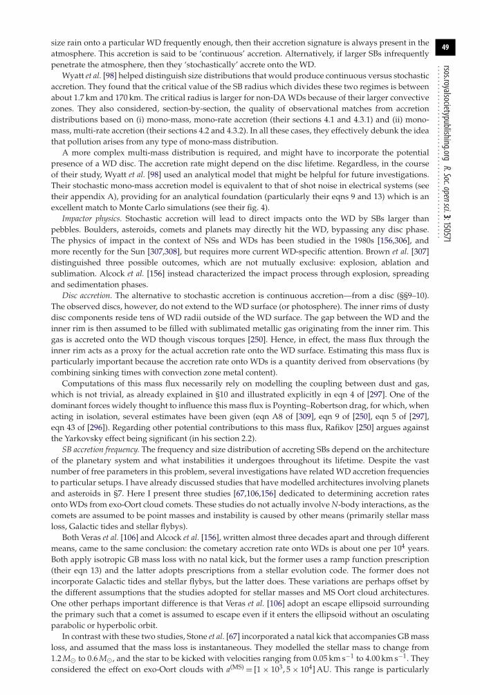
49


................................................size rain onto a particular WD frequently enough, then their accretion signature is always present in theatmosphere. This accretion is said to be ‘continuous’ accretion. Alternatively, if larger SBs infrequentlypenetrate the atmosphere, then they ‘stochastically’ accrete onto the WD.

Wyatt et al. [98] helped distinguish size distributions that would produce continuous versus stochasticaccretion. They found that the critical value of the SB radius which divides these two regimes is betweenabout 1.7 km and 170 km. The critical radius is larger for non-DA WDs because of their larger convectivezones. They also considered, section-by-section, the quality of observational matches from accretiondistributions based on (i) mono-mass, mono-rate accretion (their sections 4.1 and 4.3.1) and (ii) mono-mass, multi-rate accretion (their sections 4.2 and 4.3.2). In all these cases, they effectively debunk the ideathat pollution arises from any type of mono-mass distribution.

A more complex multi-mass distribution is required, and might have to incorporate the potentialpresence of a WD disc. The accretion rate might depend on the disc lifetime. Regardless, in the courseof their study, Wyatt et al. [98] used an analytical model that might be helpful for future investigations.Their stochastic mono-mass accretion model is equivalent to that of shot noise in electrical systems (seetheir appendix A), providing for an analytical foundation (particularly their eqns 9 and 13) which is anexcellent match to Monte Carlo simulations (see their fig. 4).

Impactor physics. Stochastic accretion will lead to direct impacts onto the WD by SBs larger thanpebbles. Boulders, asteroids, comets and planets may directly hit the WD, bypassing any disc phase.The physics of impact in the context of NSs and WDs has been studied in the 1980s [156,306], andmore recently for the Sun [307,308], but requires more current WD-specific attention. Brown et al. [307]distinguished three possible outcomes, which are not mutually exclusive: explosion, ablation andsublimation. Alcock et al. [156] instead characterized the impact process through explosion, spreadingand sedimentation phases.

Disc accretion. The alternative to stochastic accretion is continuous accretion—from a disc (§§9–10).The observed discs, however, do not extend to the WD surface (or photosphere). The inner rims of dustydisc components reside tens of WD radii outside of the WD surface. The gap between the WD and theinner rim is then assumed to be filled with sublimated metallic gas originating from the inner rim. Thisgas is accreted onto the WD though viscous torques [250]. Hence, in effect, the mass flux through theinner rim acts as a proxy for the actual accretion rate onto the WD surface. Estimating this mass flux isparticularly important because the accretion rate onto WDs is a quantity derived from observations (bycombining sinking times with convection zone metal content).

Computations of this mass flux necessarily rely on modelling the coupling between dust and gas,which is not trivial, as already explained in §10 and illustrated explicitly in eqn 4 of [297]. One of thedominant forces widely thought to influence this mass flux is Poynting–Robertson drag, for which, whenacting in isolation, several estimates have been given (eqn A8 of [309], eqn 9 of [250], eqn 5 of [297],eqn 43 of [296]). Regarding other potential contributions to this mass flux, Rafikov [250] argues againstthe Yarkovsky effect being significant (in his section 2.2).

SB accretion frequency. The frequency and size distribution of accreting SBs depend on the architectureof the planetary system and what instabilities it undergoes throughout its lifetime. Despite the vastnumber of free parameters in this problem, several investigations have related WD accretion frequenciesto particular setups. I have already discussed studies that have modelled architectures involving planetsand asteroids in §7. Here I present three studies [67,106,156] dedicated to determining accretion ratesonto WDs from exo-Oort cloud comets. These studies do not actually involve N-body interactions, as thecomets are assumed to be point masses and instability is caused by other means (primarily stellar massloss, Galactic tides and stellar flybys).

Both Veras et al. [106] and Alcock et al. [156], written almost three decades apart and through differentmeans, came to the same conclusion: the cometary accretion rate onto WDs is about one per 104 years.Both apply isotropic GB mass loss with no natal kick, but the former uses a ramp function prescription(their eqn 13) and the latter adopts prescriptions from a stellar evolution code. The former does notincorporate Galactic tides and stellar flybys, but the latter does. These variations are perhaps offset bythe different assumptions that the studies adopted for stellar masses and MS Oort cloud architectures.One other perhaps important difference is that Veras et al. [106] adopt an escape ellipsoid surroundingthe primary such that a comet is assumed to escape even if it enters the ellipsoid without an osculatingparabolic or hyperbolic orbit.

In contrast with these two studies, Stone et al. [67] incorporated a natal kick that accompanies GB massloss, and assumed that the mass loss is instantaneous. They modelled the stellar mass to change from1.2 M� to 0.6 M�, and the star to be kicked with velocities ranging from 0.05 km s−1 to 4.00 km s−1. Theyconsidered the effect on exo-Oort clouds with a(MS) = [1 × 103, 5 × 104] AU. This range is particularly

50


................................................interesting because it lies at the limit between adiabaticity and non-adiabaticity in the non-instantaneousmass ejecta case [208,210]. One can observe the straddling of this boundary in fig. 3 of [67]. Theyultimately find that this combination of instantaneous mass loss and kick succeeds in producing cometson near-parabolic orbits so that at least some will enter the ice line and sublimate.

None of these three studies modelled interstellar comets. Veras et al. [106] justify this neglect (see theirsection 3) by (i) estimating that a typical exo-Oort cloud should be a few orders of magnitude more densethan the interstellar medium, (ii) estimating that Oort cloud comet velocities are likely to be less than anorder of magnitude smaller than those of interstellar comets and (iii) pointing out that no Sun-grazingcomet has ever been observed to harbour a hyperbolic orbit.

Spectral simulations. An exciting alternative, complementary method to measure the chemicalcomposition of planetary remnants through accreted material is to derive the chemical composition of theobserved dusty [118,119] and gaseous [310,311] components of WD discs (as opposed to the atmosphericpollution) by simulating their spectra. However, successful models for the gaseous discs require knowingthe origin of the heating, particularly for the Ca II emission lines. The accretion rate derived by Hartmannet al. [310] (1017 − 1018 g s−1) is too high by several orders of magnitude to match observations. For dustydiscs, fig. 14 of [88] compared abundances derived from infrared spectra and atmospheric analyses; theJames Webb Space Telescope (JWST) should provide much better constraints.

12. Other dynamics12.1. General relativityThe sub-AU scales of WD debris discs, and the multi-AU scales of the orbits of disc progenitors, suggestthat general relativity (GR) may play a significant role in the secular evolution of remnant planetarysystems. GR does alter a, e and ω on orbital timescales [312], which can be important for volatile-rich SBswith orbital pericentres close to the disruption radius [254]. On secular timescales, a and e do not change,but ω famously does. GR will cause precession of the argument of pericentre over one full orbit on thetimescale

t(GR)ω ≈ 107 years

(M�

0.60 M�

)−3/2 ( a1.00R�

)5/2(1 − e2) (12.1)

≈ 0.15 Myr(

M�

0.60 M�

)−3/2 ( a1.00 AU

)5/2[

1 − e2

1 − 0.9992

]. (12.2)

Equations (12.1) and (12.2) may be useful, respectively, for WD debris discs and their potentially highly-eccentric progenitors.

12.2. MagnetismUnipolar inductors. Magnetic WDs may provide newfound opportunities to detect post-MS planets.Willes & Wu [46,313] demonstrated how terrestrial planets orbiting WDs with a period of less than about30 h may be detectable as electron-cyclotron maser sources. Both papers invoke the unipolar inductormodel for WD–planet pairs [137], where a circuit is formed between the conducting planet (or planetcore)—which would be inside of the WD magnetosphere—and the poles of the WD. Consequently, theWD atmosphere is heated. This scenario is visualized in figs 1–2 of [137], fig. 1 of [313] and fig. 1 of [46].

Within this framework, Willes & Wu [46,313] made an analogy with the detectable radio emissionsfrom Jupiter due to its magnetic interaction with Galilean moons. For WD planetary systems, Jupiterwould be replaced with the magnetic WD. The discovery space of WDs by this method is presented infig. 2 of [46], and is a function of WD magnetic moment and SB orbital period.

One consequence of the unipolar inductor model is magnetically induced drag on the planet (or largeenough SB to be a conductor). This interaction can cause an inward migration, with an inward drift speedof (eqn 7 of [137])

v(drift) = 4Wr2

GM�MSB, (12.3)

where W is the heating rate associated with the current. Li et al. [137] claimed that the drift is negligiblefor r � 200R�. Within this distance, the SB might already be undergoing tidal breakup (see §9). Whetherthere exist a planet-mass SB which represents this type of unipolar conductor orbiting the magnetic WDnamed GD 356 is an open question. If so, Wickramasinghe et al. [25] claimed that the planet is then likelyto have a second-generation origin, in particular from the remnants of a WD–WD merger.

51


................................................Accretion onto compact objects. Some metal-rich WDs are magnetic [105]. None of these stars have

observed discs. Therefore, the pollution could arise from stochastic accretion of neutral material thatis not affected by magnetism. Hollands et al. [105] asserted that rocky debris would be largely unaffectedby even a large magnetic field, although Metzger et al. [296] claimed that a sufficiently strong field couldaffect solid body accretion by inductive coupling.

Alternatively, impactors might sublimate and produce charged gas. In order for this gas to be accreted,it must orbit faster than the magnetosphere at the Alfvén radius [194]. Further, this gas would be accretedalong magnetic field lines. The Alfvén radius, rAlf, for a typical accreting WD is (eqn 63 of [296])

rAlf ≈(

3B2�R6

�

2M�

√GM�

)2/7

(12.4)

≈ 1.2R�(

B�

kG

)4/7(

M�

108 g s−1

)−2/7 (R�

0.01R�

)12/7 ( M�

0.6 M�

)−1/7, (12.5)

where B� is the star’s magnetic field.Planetary atmospheres. A planet’s or large moon’s magnetic field could act as a form of protection

from erosion, which might otherwise proceed rapidly. Bear & Soker [289] posed that magnetic fields cansuppress evaporation from an SB’s atmosphere due to post-MS stellar radiation. They claimed that thissuppression will occur when the ram pressure of the outflowing gas is less than the magnetic pressure.This relation leads to the following condition for the evaporation to be suppressed (their eqn 4)

B(crit)SB �

2√

MSBvwind

RSB(12.6)

≈ 5.5 × 10−3 kG

(MSB

1010 kg s−1

)1/2 (RSB

0.8R⊕

)−1 (vwind

2 × 103 m s−1

)−1, (12.7)

where BSB is the SB’s magnetic field.Other effects. Three other important points about magnetism are: (i) currents in the atmospheres of SB

may be driven by electric fields which are induced by stellar winds crossing the magnetic fields [131],(ii) for CE evolution, as an SB companion spirals in, it could spin up the envelope, consequently moredifferential rotation could enhance magnetic fields, which could represent a driver for the mass loss [51],(iii) Nordhaus & Spiegel [242] speculated that if the stellar wind is magnetically coupled to the source,then this coupling might affect both the mass loss rate and the star’s moment of inertia. The latter couldaffect tidal interactions with SBs which are brown dwarfs or massive planets (see §5).

12.3. External influencesPlanetary systems are not isolated entities. They are embedded within a galaxy and are subject to flybysand global tidal forces. These ‘external’ forces may play a crucial role in exosystem evolution. The largerthe value of r, the greater chance the chance that an SB’s evolution will be affected by these external forces.Post-MS mass loss will increase the value of r by at least a few, and possibly by orders of magnitude.Therefore, an MS system not influenced by tides or flybys might become so after the parent star hasbecome a WD or NS.

Galactic tides. Veras et al. [80] quantified external influences in the midst of post-MS mass loss. Theyfound that AGB mass loss occurs on a short-enough timescale to be decoupled from the influence ofGalactic tides (their fig. 1) but not necessarily stellar flybys. This result holds everywhere in the MilkyWay galaxy. During the WD phase, however, Galactic tides can play a significant role [260]. Further,Galactic tides has its own ‘adiabatic’ regime, where adiabatic refers to conservation of semi-major axis,and the adiabatic/non-adiabatic regime is much further away (at approx. 105 AU). Consequently, anySB near this boundary is already in the mass loss-based non-adiabatic regime. Their fig. 5 presentsa flowchart of evolutionary possibilities, and their table 1 provides equations for the adiabatic andnon-adiabatic SB evolution due to Galactic tides.

Hill ellipsoid. Galactic tides carve a region around the primary within which SBs orbit the primaryand not the centre of the Galaxy. This region, which is not a sphere, is known as the Hill ellipsoid, withdimensions provided by eqns 21–22 of [80]. The Hill ellipsoid lies close to the adiabatic/non-adiabaticGalactic tidal boundary, and can help determine, for example, which Oort cloud comets escape before,during and after GB evolution [106]. For M(MS)

� = 2 M�, about three-quarters of the volume of the entire

52


................................................MS Hill ellipsoid includes the semi-major axis range for which post-MS mass loss will cause an SBto escape.

Stellar flybys. Although stellar flybys are unpredictable, the stellar space density in the Milky Way ishigh enough to expect a close encounter at a few hundred AU over a typical Solar-like MS lifetime. Thecloser to the centre of Galaxy the star-SB system resides, the more susceptible it is to flybys. Fig. 3 of [80]quantifies the expected close encounter distance, and many of the above notions in this section; note thatmost known exoplanets reside at approximately 8 kpc from the Galactic centre.

Wide stellar binaries. Galactic tides trigger close encounters between wide binary systems for the firsttime many Gyr into the WD phase of the initially more massive star. This encounter in turn triggersinstabilities in extant, and perhaps formerly quiescent, planetary systems around one or both stars [260].This mechanism provides an avenue to pollute WDs which are many Gyr old. Importantly, the mass lossexperienced in the post-MS evolution of the more massive star is adiabatic with respect to its daughterplanetary system, but non-adiabatic with respect to the stellar binary companion. Consequently, the finalsuper-adiabatic binary separation will be affected by Galactic tides and create eccentricity changes.

12.4. Climate and habitabilityCan habitable climates exist on SBs orbiting compact objects? At least a few studies [143,145,242,314]have explored this possibility in some detail. In just about every case, the SB is assumed to have tidallycircularized around the compact object. Agol [145] claimed that planets in the WD continuously habitablezones with orbital periods of ≈4 − 32 h will be circularized and tidally locked in ≈10 − 1000 years.

Fossati et al. [143] used a modified radiative transfer model to demonstrate that photosyntheticprocesses can be self-sustaining on planets in a continuously habitable zone around a non-magnetic WD.WDs provide stable luminosity sources with ultraviolet radiation doses which may be less damagingthan those of MS stars. Although the WD luminosity continuously decreases, Fossati et al. [143] claimedthat while a WD cools from 6000 K to 4000 K, a planet which is about 0.01 AU distant can remain in thehabitable zone for about 8 Gyr, sufficiently long to allow complex life to develop.

Alternatively, Agol [145] performed computations of one-dimensional radiative–convectiveatmosphere models with water loss at the inner edge and a maximum carbon dioxide greenhouse at theouter edge. Barnes & Heller [314] adopted multiple tidal models, and found that a WD’s strong extremeultraviolet emission is a significant barrier to sustain life. Nordhaus & Spiegel [242] estimated that if aplanet is perturbed close enough to a WD to be tidally circularized (as in Veras & Gänsicke [144]), thenthe amount of orbital energy dissipated as heat, I, would be (their eqn 6)

I ∼ −4 × 1035 J(

M�

0.6 M�

)(MSB

M⊕

)(a

R�

)−1, (12.8)

enough to scupper the prospects for habitability. Agol [145] also considered the prospects of other SBsdelivering volatiles to a planet after it entered the WD habitable zone (a realistic possibility: see e.g. [67,106,156]), and Nordhaus & Spiegel [242] estimated that the impacts would impart orders of magnitudemore of specific energy to those planets than the impacts which wiped out the dinosaurs.

Finally, Perets [279] mentioned that second-generation formation can provide new developmentalpathways for habitable planets unavailable to first-generation planets, and Spiegel & Madhusudhan [131]speculated that a giant planet’s atmosphere could be carbon-enriched during the GB phases by accretinga stellar wind from a star that has undergone third dredge-up. Similarly, the chemical imprint of accretionin a terrestrial planet’s atmosphere during the GB phase might affect habitability during the WD phase.

13. The fate of the Solar systemThe post-MS fate of the Solar system is of intrinsic human interest; Sackmann et al. [315] ‘could notresist exploring the Sun’s future’. However, the conclusions of the studies that investigated this futuredo not agree, highlighting the need for additional work in this area. The Solar system consists of fourterrestrial planets, four giant planets, many asteroids, comets and moons, and many more smaller SBs.The gravitational influence of the Sun extends to 1 × 105 − 3 × 105 AU (eqns 21–22 of [80]), with objectslikely existing out to that edge through the Oort cloud. In short, the fate of the Solar system is complex.

Tackling this problem requires all relevant forces to be brought to bear (figure 2). A planet willsimultaneously expand its orbit, accrete stellar ejecta, evaporate from stellar radiation and be tidallyinfluenced from Solar tides. Each planet will experience these effects to different extents, but are

53


................................................close enough to the Sun (a � 30 AU) such that external influences are negligible, and are large enough(RSB > 103 km) to not be bothered by stellar wind drag, the Yarkovsky or YORP effects.

Remainder of main sequence. Barring a close stellar flyby, the current gross architecture of the Solarsystem should be maintained throughout the remainder of the MS. Although the outer four planets willremain stable until the end of the MS, there is a one to few percent chance that the inner four planetswill become collisional and/or unhinged [255,316]. The asteroid and Kuiper belt will likely continue tocollisionally deplete.

Mercury and Venus. All studies agree that Mercury will be engulfed. The Sun’s surface will expandto such a great extent (to approx. 1 AU) that even Mercury’s expanded orbit (at approx. 0.8 AU) wouldlie within the Sun’s GB surface. Venus will almost certainly suffer a similar fate, despite the findingsof Sackmann et al. [315], because of Sun–planet tides [229,230]. Because Sackmann et al. [315] did notincorporate tidal effects in their analysis, Venus’ expanded orbit (at approx. 1.5 AU) does escape theSun’s reach in that (physically unrealistic) scenario.

Earth. The Earth’s fate is sensitive to both the Solar model and tidal model adopted. Schröder &Smith [230], using the updated Reimers mass loss prescription from equation (2.1) and the tidalformalism of Zahn [239,245], found that the Earth will be engulfed unless all tweakable parameterswithin the model were at one edge of their uncertainty ranges. They predict that Mercury, Venus andEarth will all be engulfed about 4.3, 1.5 and 0.5 Myr before the Sun’s RGB phase ends, which will occurabout 7.59 Gyr from now. If Earth does survive, it won’t be habitable. The post-MS state of its atmosphereand surface has not though been modelled in detail. Schröder & Smith [230] do speculate that the Solarsystem’s habitable zone during the RGB tip would extend from about 49 to 71 AU, beyond the currentlocation of Neptune.

Outer 5 planets and asteroid belt. Mars and the giant planets will survive, but the asteroid belt willlikely not. Dynamically, the giant planets will not undergo instability [223] and experience a quiescentexistence around the Solar WD. Mars should also survive dynamically because the semi-major axis ratioof Jupiter and Mars is greater than 3, and that ratio will be maintained during post-MS evolution due toadiabatic mass loss. Physically, how these five planets will fare has only started to be explored. Villaver &Livio [52] warned that planets in Jupiter’s location might undergo significant evaporation. Spiegel &Madhusudhan [131] specifically considered the fate of Jupiter’s atmosphere: how it is chemically andthermally altered by Solar wind accretion and the Sun’s GB radiation. SBs in the asteroid belt will eitherbe evaporated or spun up to fission [251] given their close proximity to the Sun.

Moons. The moons of the Solar system have diverse physical characteristics and orbit theirparent planets out to about half of one Hill radius. These orbits will become more stable after theSun has become a WD because of the effect of mass loss on Hill radius (see equation (7.5)) andbecause the remaining planets are not expected to undergo potentially disruptive scattering [268]. Theconsequences of GB radiation on the ice crusts and oceans of moons like Europa and Enceladus remainunexplored.

Kuiper belt and scattered disc. How the Kuiper belt and scattered disc will be altered by post-MSSolar evolution remains unclear. The re-distribution of Kuiper belt objects due to the Yarkovsky effect,even if slight, may affect the edges of the belt and the resonant characteristics of many of these objectswith Neptune. Consequently, the extent of the depletion [59,61,259] might change from current levels.An expanded scattered disc would be more susceptible to dynamical reshuffling from stellar flybys,particularly over several Gyr during the Solar WD phase (fig. 3 of [80]). The critical MS distance at whichscattered disc objects might escape during post-MS phases is between 103 and 104 AU [210].

Oort cloud. The Oort cloud will be dynamically excited by the combination of stellar mass loss, orbitalexpansion, Galactic tides and stellar flybys [80]. The latter two will change from their present dayprescriptions because the Milky Way and the Andromeda galaxies will collide before the Sun turns off ofthe MS [317]. Veras et al. [106] and Alcock et al. [156] disagree on the extent to which Oort clouds wouldbe depleted during the GB phase, but interestingly are in rough agreement about the number of thesecomets reaching the inner Solar system (approx. 1 in every 104 years). The distribution of ejected cometswould not necessarily scale with semi-major axis [210] and the subsequent interactions with survivingplanets has not been considered in detail.

14. Numerical codesPost-MS planetary science has benefited with improvement in numerical tools since the discovery ofthe PSR 1257+12 planets. The two most widely used classes of tools for this science are stellar evolution

54


................................................Table 2. Some numerical codes used by cited investigations. ‘Type’ refers to either a stellar evolution code, or an N-body dynamics code,or both.

name type ref used by

AMUSE both [318] [276]. . . . . . . . . . . . . . . . . . . . . . . . . . . . . . . . . . . . . . . . . . . . . . . . . . . . . . . . . . . . . . . . . . . . . . . . . . . . . . . . . . . . . . . . . . . . . . . . . . . . . . . . . . . . . . . . . . . . . . . . . . . . . . . . . . . . . . . . . . . . . . . . . . . . . . . . . . . . . . . . . . . . . . . . . . . . . . . . . . . . . . . . . . . . . . . . . . . . . . . . . . . . . . . . . . . . . . . . .

BSE stellar [221] [176,278]. . . . . . . . . . . . . . . . . . . . . . . . . . . . . . . . . . . . . . . . . . . . . . . . . . . . . . . . . . . . . . . . . . . . . . . . . . . . . . . . . . . . . . . . . . . . . . . . . . . . . . . . . . . . . . . . . . . . . . . . . . . . . . . . . . . . . . . . . . . . . . . . . . . . . . . . . . . . . . . . . . . . . . . . . . . . . . . . . . . . . . . . . . . . . . . . . . . . . . . . . . . . . . . . . . . . . . . . .

MESA stellar [319,320] [131,226,241]. . . . . . . . . . . . . . . . . . . . . . . . . . . . . . . . . . . . . . . . . . . . . . . . . . . . . . . . . . . . . . . . . . . . . . . . . . . . . . . . . . . . . . . . . . . . . . . . . . . . . . . . . . . . . . . . . . . . . . . . . . . . . . . . . . . . . . . . . . . . . . . . . . . . . . . . . . . . . . . . . . . . . . . . . . . . . . . . . . . . . . . . . . . . . . . . . . . . . . . . . . . . . . . . . . . . . . . . .

SSE stellar [27] [24,32,144,264,277]. . . . . . . . . . . . . . . . . . . . . . . . . . . . . . . . . . . . . . . . . . . . . . . . . . . . . . . . . . . . . . . . . . . . . . . . . . . . . . . . . . . . . . . . . . . . . . . . . . . . . . . . . . . . . . . . . . . . . . . . . . . . . . . . . . . . . . . . . . . . . . . . . . . . . . . . . . . . . . . . . . . . . . . . . . . . . . . . . . . . . . . . . . . . . . . . . . . . . . . . . . . . . . . . . . . . . . . . .

STAREVOL stellar [321] [228]. . . . . . . . . . . . . . . . . . . . . . . . . . . . . . . . . . . . . . . . . . . . . . . . . . . . . . . . . . . . . . . . . . . . . . . . . . . . . . . . . . . . . . . . . . . . . . . . . . . . . . . . . . . . . . . . . . . . . . . . . . . . . . . . . . . . . . . . . . . . . . . . . . . . . . . . . . . . . . . . . . . . . . . . . . . . . . . . . . . . . . . . . . . . . . . . . . . . . . . . . . . . . . . . . . . . . . . . .

STARS stellar [322] [25,230]. . . . . . . . . . . . . . . . . . . . . . . . . . . . . . . . . . . . . . . . . . . . . . . . . . . . . . . . . . . . . . . . . . . . . . . . . . . . . . . . . . . . . . . . . . . . . . . . . . . . . . . . . . . . . . . . . . . . . . . . . . . . . . . . . . . . . . . . . . . . . . . . . . . . . . . . . . . . . . . . . . . . . . . . . . . . . . . . . . . . . . . . . . . . . . . . . . . . . . . . . . . . . . . . . . . . . . . . .

HERMITE N-body [323] [277]. . . . . . . . . . . . . . . . . . . . . . . . . . . . . . . . . . . . . . . . . . . . . . . . . . . . . . . . . . . . . . . . . . . . . . . . . . . . . . . . . . . . . . . . . . . . . . . . . . . . . . . . . . . . . . . . . . . . . . . . . . . . . . . . . . . . . . . . . . . . . . . . . . . . . . . . . . . . . . . . . . . . . . . . . . . . . . . . . . . . . . . . . . . . . . . . . . . . . . . . . . . . . . . . . . . . . . . . .

MERCURY Bulirsch-Stoer N-body [324] [24,59,61,106,144,208,264,325]. . . . . . . . . . . . . . . . . . . . . . . . . . . . . . . . . . . . . . . . . . . . . . . . . . . . . . . . . . . . . . . . . . . . . . . . . . . . . . . . . . . . . . . . . . . . . . . . . . . . . . . . . . . . . . . . . . . . . . . . . . . . . . . . . . . . . . . . . . . . . . . . . . . . . . . . . . . . . . . . . . . . . . . . . . . . . . . . . . . . . . . . . . . . . . . . . . . . . . . . . . . . . . . . . . . . . . . . .

MERCURY Hybrid N-body [324] [61,271,273,275,326]. . . . . . . . . . . . . . . . . . . . . . . . . . . . . . . . . . . . . . . . . . . . . . . . . . . . . . . . . . . . . . . . . . . . . . . . . . . . . . . . . . . . . . . . . . . . . . . . . . . . . . . . . . . . . . . . . . . . . . . . . . . . . . . . . . . . . . . . . . . . . . . . . . . . . . . . . . . . . . . . . . . . . . . . . . . . . . . . . . . . . . . . . . . . . . . . . . . . . . . . . . . . . . . . . . . . . . . . .

MERCURY Radau N-body [324] [259,260]. . . . . . . . . . . . . . . . . . . . . . . . . . . . . . . . . . . . . . . . . . . . . . . . . . . . . . . . . . . . . . . . . . . . . . . . . . . . . . . . . . . . . . . . . . . . . . . . . . . . . . . . . . . . . . . . . . . . . . . . . . . . . . . . . . . . . . . . . . . . . . . . . . . . . . . . . . . . . . . . . . . . . . . . . . . . . . . . . . . . . . . . . . . . . . . . . . . . . . . . . . . . . . . . . . . . . . . . .

PKDGRAV N-body [327] [59,295]. . . . . . . . . . . . . . . . . . . . . . . . . . . . . . . . . . . . . . . . . . . . . . . . . . . . . . . . . . . . . . . . . . . . . . . . . . . . . . . . . . . . . . . . . . . . . . . . . . . . . . . . . . . . . . . . . . . . . . . . . . . . . . . . . . . . . . . . . . . . . . . . . . . . . . . . . . . . . . . . . . . . . . . . . . . . . . . . . . . . . . . . . . . . . . . . . . . . . . . . . . . . . . . . . . . . . . . . .

codes and N-body codes. In table 2, I list codes that have been used in references from this paper. Anotherclass of codes not listed are model atmosphere codes, like the IRAP and La Plata codes used by Deal etal. [302].

Full-lifetime integrations over the entire MS, GB and much of the WD or NS phases remaincomputationally challenging for several reasons: (i) the simulations often require a method to combinean N-body code with a stellar evolution code, (ii) this combination should ensure that errors convergeas timesteps decrease (consider fig. 1 of [24]), (iii) the additional relevant forces from figure 2 needto be included and (iv) the bodies (stellar and SBs) must be on sufficiently wide orbits, otherwise thesimulations will take months or years of real time to finish. Fortunately, the transition from MS to WDexpands the orbits of surviving SBs and decreases the parent mass, allowing for quicker integrationsby an order of magnitude (see fig. 8 of [24]). Consequently, the shorter the MS lifetime, and the largerthe value of M(MS)

� , the more quickly the simulations will finish. Although energy is not a conservedquantity, angular momentum typically is, and represents an important benchmark for accuracy. Strongclose encounters between SBs increase angular momentum errors (footnote #7 of [144]).

Two recent N-body codes which may prove useful for future studies are the GENGA code [328] andIAS15 code [329]. GENGA uses graphical processing units (GPUs) to speed up computations. Theyclaim their code runs up to 30 times faster than MERCURY and 8 times faster than PKDGRAV2, andcan handle up to 2048 massive bodies or 106 test particles. IAS15 is a 15th-order N-body integrator thatcan handle close encounters, high-eccentricity orbits and non-conservative forces, with systematic errorsbelow machine precision. Section 1 of Rein & Spiegel [329] usefully explains the concept of symplecticity,and how symplectic integrators encounter difficulties when modelling binary systems or incorporatingnon-conservative forces.

15. Future directionsThe fast-growing field of post-MS planetary science demands that theorists and observers work inconcert to achieve shared goals, but should not obscure the importance of purely theoretical pursuitsfor such a dynamically rich and unexplored topic. In this section, I present ideas for future directions forboth groups.

15.1. Pressing observations

15.1.1. Continued monitoring of known objects

WD 1145+017. The one to several disintegrating SBs orbiting the polluted and disc-bearing WD1145+017 [125] requires vigilant monitoring (i) first to constrain the number of SBs and their masses,(ii) to detect the onset of future breakup events from the large SBs, as they reside within the disruption

55


................................................radius, (iii) to determine how the surrounding disc varies due to direct injection of material and (iv) todetect variability in the accretion rates onto the WD. A chemical analogy may also be made with theplanets breaking up around MS stars. Bochinski et al. [330] provided recent and strong evidence for alow-mass rocky planet disrupting around the MS star KIC 12557548 B, following up on the suggestionfrom Rappaport et al. [331]. Two other potentially disintegrating planets (KOI-2700b [332] and K2-22b [333]) raise the possibility even more that analysis of additional light curves from these systemscould help measure grain composition of the broken-up debris.

WD J0959-0200. Continued monitoring of the variable disc around WD J0959-0200 [115] is important.Given that the flux dropped almost 35% within a 300-day period, there is a possibility that (i)instability in the disc will create an observable flare, as predicted by Bear & Soker [294] and (ii)photospheric abundances can be measured during the flux change, which will allow us to observevariability in accretion rates. Detecting variability in accretion onto DA WDs (like WD J0959-0200) maycrucially constrain sinking timescales and disc lifetimes. Further, the WD J0959-0200 contains a gaseouscomponent, and monitoring the gas and dust simultaneously might help us understand the interplaybetween dust, gas and variability.

SDSS J1617+1620. The variability of the gaseous component of the WD disc orbiting SDSS J1617+1620since the year 2006 [334] generates the exciting possibilities that (i) potential future flare-ups due torepeated impacts of leftover debris from a tidal disruption event could be observed and (ii) we can seethe inner rim of the disc moving outward through changes in the width of Ca II lines.

SDSS J1228+1040. Following the evolution of the axisymmetric and eccentric WD gaseous and dustydisc shown in figure 7 is particularly important to constrain WD disc evolution theory. Manser et al. [122]provided a clear prediction: In December 2016, the WD debris disc in SDSS J1228+1040 should reachhalfway through its precession cycle.

NN Ser. Additional observations of NN Ser, particularly over the next couple years, will significantlyhelp pin down the constraints for the number and properties of planets in this post-CE binary. The eclipsetiming trajectory features a crest in the years 2019–2020 (fig. 9 of [175]) which will help confirm or refutethe nature of the putative planets.

15.1.2. Monitoring new objects

Giant branch planets. One of the most pressing theoretical concerns is the uncertainty about tidaldissipation mechanisms and their relation to planetary rheology. Planet-bearing GB systems can helpus constrain some of the relevant physics. The tidally-based RGB study of Villaver et al. [228] illustratedthat the region void of planets is too wide to have been depleted by tidal effects alone, providing uswith a mystery. We need observations of greater numbers of GB planets in order to obtain a moredetailed parameter distribution of these objects, and in particular to identify a cluster at the tidaldisruption edge [242]. Separately, a greater sample of GB planets will help us resolve the difference inthe planet–metallicity correlation in MS systems versus GB systems [168,169].

Massive polluted white dwarfs. How massive can host stars of exoplanets be? This fundamental questioninforms planetary formation and evolution, and current technology dictates that the answer is bestobtained through observing high-mass WDs for signatures of pollution. For example, the polluted WDSDSS J1228+1040, which also happens to be the first WD discovered with a gaseous disc component,had a likely progenitor MS mass of M(MS)

� ∼ 4 M�. No MS planet has yet been discovered around such amassive star.

Magnetic polluted white dwarfs. Planetary remnants, through split metal lines in the spectrum, helpus understand magnetism in WDs, particularly in the oldest and coolest WDs. Therefore, we need toidentify additional DZH stars [105], and further build up enough of a sample to distinguish the incidenceof magnetic hydrogen-rich and magnetic helium-rich WDs. Further, a planetary core heating up a DHWD might have optically detectable Hα emission [137].

Binary systems with white dwarfs. Kratter & Perets [277] explicitly suggested from their theoreticalresults that future surveys might find planets orbiting WDs in WD–MS binaries within the progenitorAGB radius. Further, Perets [279] claimed that WD–MS and WD–WD systems with separations of tensor hundreds of AU should be prime targets. He also provided specific examples of candidate second-generation exoplanetary systems. The likelihood of a second-generation disc formation scenario frombinary stellar winds may be assessed from the frequency of wide WD companions to WD debrisdiscs [285].

James Webb Space Telescope. Stone et al. [67] specifically studied the capacity of JWST to discover newWD debris discs, and found the prospects excellent (see their eqn 35). JWST observations of young WD

56


................................................debris discs could help distinguish an origin from exo-Oort cloud disruption versus from a remnantexo-Kuiper belt. The former would produce a different and detectable brightness profile (see section 4.4and figs 7–9 of [67]). JWST, along with SPICA, should also find older, fainter discs [112]. Further, theEuropean Mid-InfraRed Instrument on-board JWST will identify specific minerals in the debris orbitingWDs (currently G 29-38 is the only WD with a high-quality infrared spectrum; see fig. 4 of [119]),and this data can be combined with the known atomic abundances measured with HST. For pulsarplanetary systems, Shannon et al. [186] suggested that tens to hundreds of hours of JWST time coulddetect the putative asteroid disc around B1937+21. Identifying the disc is particularly important partlybecause they suggest that second-generation circumpulsar planetesimal formation may be common;JWST observations will provide the timing precision ‘noise floor’, which in turn informs us about thestability of these stars. Finally, Wang [185] claimed that the ability of a pulsar to heat up circumstellarmaterial is still unclear, and can be resolved with JWST along with WISE and the TMT.

Other telescopes. ALMA, due to its high spatial resolution, can directly resolve exo-Kuiper beltsorbiting WDs [67]. Di Stefano [335] touted the potential of gravitational lensing to discover WDplanetary systems, particularly with Pan-STARRS and LSST. The putative subdwarf planets inferredfrom pulsations may be confirmed or refuted with the PEPSI at LBT [179]. Gaia, LSST and PLATO willrepeatedly (tens to thousands of times) survey 105–106 WDs, and by the year 2020 the combined effortsof the ESA missions Gaia and Euclid will increase the number of known WD debris discs by at least anorder of magnitude. PLATO will find planets orbiting WDs. Gaia, LSST and WFIRST will help detectfree-floaters, which may help constrain the fraction of ejected planets due to mass loss [80], particularlyif high mass stars are targeted. Gaia will also provide better constraints on the wide binary population,potentially allowing for a test of the pollution mechanism suggested by Bonsor & Veras [260]. The SKAwill also aid post-MS planetary science through the radio portion of the electromagnetic spectrum: thearray will improve the chances of detection of radio emissions from WD–terrestrial planet systems [46]and help confirm the existence of circumpulsar discs [194].

Other considerations. The drastic increase then decline in luminosity from a tidal disruption event couldcreate detectable outburst events. Bear & Soker [294] made a comparison with dwarf novae (see theirtable 1), which also create outbursts. Bear & Soker [290] proposed that young, hot WDs should ionizenebulae formed from an episode of AGB reincarnation due to engulfment of planetary hydrogen. Fossatiet al. [143] suggested that polarimetry can be used to detect non-transiting WD habitable zone planetsbecause the signal would be 2–5 orders of magnitude larger than for habitable planets around typicalM-dwarf to Sun-like stars. Finally, exomoons in MS systems are on the verge of discovery; Pasqua &Khudhair [336] calculated the time-of-arrival signal that a hypothetical exomoon on an inclined orbitaround a circumpulsar planet would induce.

15.2. Theoretical endeavoursTheoretical progress is lagging behind both the mounting observations of post-MS systems and themultitude of theory papers about MS planetary systems. Post-MS systems includes rich dynamics thatis not found in MS systems (figure 2), and which needs to be explored in greater detail in order tounderstand physics and improve models.

Effects of radiation. Firstly, no study has yet self-consistently integrated the set of equations (6.1), (6.4),(6.5) and (6.6), or a similar set. Also, the applicability of the Yarkovsky geometry in equation (6.1) forhighly eccentric objects is limited. In general, w may be a function of time, even for spherical SBs. Wealso know that asteroid-sized SBs are generally not spherical, and for those objects equation (6.1) shouldbe modified. Further, equation (6.4) provides an averaged quantity. The high luminosity of GB stars andthe duration of the SB orbit may require one to model spin changes on orbital rather than just seculartimescales. We also need to characterize the debris fields produced from YORP spin-up of SBs so thatwe understand from where WD pollution arises, and can make a chemical link with first-generationformation. Equation (6.5) applies only for a single-species homogeneous sphere. We know that realasteroids are multi-layered, aspherical and contain many chemical species. In order to quantify theamount of water remaining in these SBs, more sophisticated models are required. Finally, the equationsof motion for a moon (which orbits some SB) will be different than what is presented here, partly becauseof shadowing.

How do atmospheres change from post-MS stellar radiation? An important follow-up to previousstudies [43,52,131] would be to solve the hydrodynamical equations for atmospheric escape. Further,these studies do not necessarily agree about the extent of Jupiter’s atmosphere that will escape. How

57


................................................much will Saturn, Uranus and Neptune be ablated? We know that the four giant planets in the Solarsystem will remain on stable orbits during the Solar GB phase, but how will they physically evolve?

Effects of tides. As is also true for MS tidal studies, tidal investigations for GB, WD and NSs canbe improved by sampling tidal dissipation prescriptions for different planetary rheologies and stellarstructures. Doing so will better constrain the timescales for SB destruction and the critical engulfmentradius. Treating a population of known exoplanets with similar prescriptions (as in fig. 4 of [242]) mightyield a very different result than a more individualized treatment of each planet (fig. 15 and table 2of [337]). For GB systems, equations (5.1) and (5.2) need to be extended to higher SB eccentricities, andpotentially coupled with stellar spin dynamics [242] at those higher eccentricities. For stars with similarradial extensions during both the RGB and AGB phases, different tidal prescriptions may apply [30,228]and might need to be treated together self-consistently within a single simulation.

Effects of mass loss. Compared with radiation and tides, our understanding of how SBs evolve due tostellar mass loss is better. Nevertheless, the consequences of accretion onto SBs has largely been ignored,as has the potential for GB stars to experience kicks during non-instantaneous mass loss. The effects ofram pressure and entrainment on smaller SBs such as boulders and pebbles need better quantification.How these effects, along with frictional drag, affect the transition between adiabatic and non-adiabaticmotion is not yet clear. The transition itself, even in the non-accreting case, needs further explorationin order to explain e.g. the non-monotonic behaviour in fig. 10 of [210]. How resonances are formed,broken and maintained [215] may crucially affect WD pollution rates [59] and need further analysis ona commensurability-by-commensurability basis. Finally, simulations of the long-term MS future of theSolar system typically do not include effects from MS Solar mass loss. Although small, mass loss duringthe MS will cause a shift much greater than the instability-inducing 0.38 mm shift suggested by Laskar& Gastineau [255].

Different planetary architectures. So far, self-consistent full-lifetime numerical simulations of planetarysystems have been limited in scope in terms of number of bodies, amount of time simulated and numberof simulations. Room for improvement is significant, but must overcome computational hurdles. Weneed post-MS multi-planet simulations with an asteroid or Kuiper belt, a situation that will mirror thefate of our own Solar system. The planetary mass which maximizes the accretion rate onto the eventualWD is still unknown [61]. Where is the sweet spot for one-planet and other configurations? We need todetermine the orbital and physical evolution of post-MS exomoons, Trojan asteroids and exorings, andhow they will be subject to close encounters from other objects. We need to determine how fragmentsfrom SB–SB collisions evolve and are subject to scattering events. Mustill et al. [264] estimated throughsimulations of three planets only that no more than 1% of WDs should eventually host close-in giantsplanets. We must improve that estimate with (i) terrestrial-mass planets, (ii) unequal-mass planets and(iii) SBs smaller than planets. Also, further exploration of binary and triple stellar planet-hosting systems[62,280] will provide us with a more representative, population-based perspective on the evolution ofplanetary systems in the Milky Way.

Investigations detailing the fates of specific known exoplanetary systems are lacking. The famousHR 8799 system has a parent star with a progenitor mass that is typical of the currently observed WDpopulation (figure 3) and represents a potential exemplar for polluted WD systems. The fates of otherwide-orbit multi-planet systems on the current edge of MS stability (see e.g. section 6.3 of [24]) are notyet clear.

Second-generation formation. Currie & Hansen [287] called for more sophisticated extensions oftheir models of second-generation circumpulsar disc formation. In their section 7, they list severalsimplifications and assumptions adopted, which have not yet been lifted nearly a decade after that paperhas been published. Many of the recent advancements in first-generation planet formation theory wouldalso be applicable to second-generation SB formation.

White dwarf debris disc formation and evolution. The details of tidal disruption of an SB entering theWD Roche radius (and forming a disc) should be improved, particularly given the fine detail of someobservations like those of Manser et al. [122] and in figure 7. As mentioned by Veras et al. [295], improvedN-body rubble pile simulations may include ‘soft spheres’, with rolling and twisting friction betweenparticles at multiple points of contact [338]. Alternatively, the spheres could have internal strength, ornot be in the shapes of spheres at all. Movshovitz et al. [339] instead used polyhedral regular or orirregular grains to represent the building blocks of SBs. The SBs can be different shapes and spins, andwhen appropriate, harbour different equations of state [291]. Numerical modelling of the disruption ofan incoming SB at an already existing disc would help characterize this likely scenario.

The evolution of the disc requires coupled modelling of the dust and gas, as in Metzger et al. [296].They provided many useful relations which may be used for further modelling. Considering the simpler

58


................................................case of gas only, with potential self-generation of eccentricity and precession, is another approach whichmay help us disentangle different effects in these complex systems. Further work on spectral modellingof these discs [310,311] can link their composition with orbital evolution.

WD accretion. Improvements in atmospheric modelling will allow us to better distinguish accretedmaterial from radiatively levitated material in hot WDs and from dredged-up carbon in cool WDs. Inconcert with observations, modelling the onset and tail-off of accretion events with different functionalforms than equation (11.1) and as a function of chemical elements may help us better constrain progenitormasses and evaluate the steady-state assumption in DBZ WDs. Accretion from direct collisions betweenan SB and WD needs to be explored in more detail, to distinguish fragmentation, sublimation andexplosion regimes.

Finally. Will the Sun become a polluted WD? The chances are good, with multiple surviving planetspotentially perturbing Kuiper belt and asteroid belt fragments onto the Solar WD. However, otherpolluted WDs will have harboured different planetary architectures on the MS. Extrasolar planets, firstunknowingly seen inside of a WD [3] and then by their own right orbiting a pulsar [1], have taught us that‘their diversity cannot be easily foreseen from extrapolations of our knowledge of the Solar System’ [180].

Competing interests. I have no competing interests.Funding. This research benefited by support from both the European Union through ERC grant no. 320964 and theRoyal Society through grant no. IE140641.Acknowledgements. I solicited input on this manuscript from many researchers, from graduate students to seniorprofessors, and was rewarded with valuable comments and perspectives that improved the final product. WilliamF. McDonough provided initial stage advice, and later the following individuals provided explicit suggestionsfor text, equations and physics: Siegfried Eggl, Jay Farihi, Boris T. Gänsicke, Nikolaos Georgakarakos, Mark A.Hollands, Michael Jura, Detlev Koester, Christopher J. Manser, Thomas R. Marsh, Noam Soker, Nicholas C. Stone,Pier-Emmanuel Tremblay, Andrew Vanderburg, David J. Wilson and Siyi Xu. Boris T. Gänsicke and Jay Farihi kindlyprovided updated data for, respectively, figures 5 and 6. I also appreciate the referee’s comments, which helpedimprove the narrative.

References1. Wolszczan A, Frail DA. 1992 A planetary system

around the millisecond pulsar PSR1257+12. Nature355, 145–147. (doi:10.1038/355145a0)

2. Wolszczan A. 1994 Confirmation of Earth-massplanets orbiting the millisecond pulsar PSRB1257+12. Science 264, 538–542. (doi:10.1126/science.264.5158.538)

3. van Maanen A. 1917 Two faint stars with largeproper motion. Publ. Astron. Soc. Pac. 29, 258–259.(doi:10.1086/122654)

4. van Maanen A. 1919 Stellar parallaxes derived fromphotographs made with the 60-inch reflector ofthe Mount Wilson Observatory. Astron. J. 32,86–88. (doi:10.1086/104334)

5. Campbell B, Walker GAH, Yang S. 1988 A search forsubstellar companions to solar-type stars.Astrophys. J. 331, 902–921. (doi:10.1086/166608)

6. Latham DW, Mazeh T, Stefanik RP, Mayor M, BurkiG. 1989 The unseen companion of HD114762: aprobable brown dwarf. Nature 339, 38–40.(doi:10.1038/339038a0)

7. Mayor M, Queloz D. 1995 A Jupiter-masscompanion to a solar-type star. Nature 378,355–359. (doi:10.1038/378355a0)

8. Marcy GW, Butler RP. 1996 A planetary companionto 70 virginis. Astrophys. J. 464, L147–L151.(doi:10.1086/310096)

9. Butler RP, Marcy GW. 1996 A planet orbiting 47Ursae Majoris. Astrophys. J. 464, L153–L156.(doi:10.1086/310102)

10. Lillo-Box J, Barrado D, Moya A et al. 2014Kepler-91b: a planet at the end of its life. Planetand giant host star properties via light-curve

variations. Astron. Astrophys. 562, A109.(doi:10.1051/0004-6361/201322001)

11. Carter-Bond JC, O’Brien DP, Delgado Mena E,Israelian G, Santos NC, González Hernández JI. 2012LowMg/Si planetary host stars and theirMg-depleted terrestrial planets. Astrophys.J. 747, L2. (doi:10.1088/2041-8205/747/1/L2)

12. Lagrange-Henri AM, Beust H, Ferlet R,Vidal-Madjar A, Hobbs LM. 1990 HR 10—a newBeta Pictoris-like star? Astron. Astrophys. 227,L13–L16.

13. Melnick GJ, Neufeld DA, Ford KES,Hollenbach DJ, Ashby MLN. 2001 Discoveryof water vapour around IRC+ 10216 asevidence for comets orbiting another star.Nature 412, 160–163. (doi:10.1038/35084024)

14. Welsh BY, Montgomery S. 2013 Circumstellargas-disk variability around A-type stars: thedetection of exocomets? Publ. Astron.Soc. Pac. 125, 759–774. (doi:10.1086/671757)

15. Kiefer F, Lecavelier des Etangs A, Augere J-C,Vidal-Madjar A, Lagrange A-M, Beust H. 2014Exocomets in the circumstellar gas disk of HD172555. Astron. Astrophys. 561, L10. (doi:10.1051/0004-6361/201323128)

16. Kiefer F, des Etangs AL, Boissier J, Vidal-Madjar A,Beust H, Lagrange A-M, Hébrard G, Ferlet R. 2014Two families of exocomets in theβ Pictorissystem. Nature 514, 462–464. (doi:10.1038/nature13849)

17. Jura M, Young ED. 2014 Extrasolar cosmochemistry.Annu. Rev. Earth Planet Sci. 42, 45–67.(doi:10.1146/annurev-earth-060313-054740)

18. Farihi J. Submitted. Circumstellar debris andpollution at white dwarf stars.

19. Iben I. 2013 Stellar evolution physics, volume 1:physical processes in stellar interiors. Cambridge,UK: Cambridge University Press.

20. Iben I. 2013 Stellar evolution physics, volume 2:advanced evolution of single stars. Cambridge, UK:Cambridge University Press.

21. Wood BE, Muller H-R, Zank GP, Linsky JL. 2002Measured mass-loss rates of solar-like stars as afunction of age and activity. Astrophys. J. 574,412–425. (doi:10.1086/340797)

22. Zendejas J, Segura A, Raga AC. 2010 Atmosphericmass loss by stellar wind from planets aroundmain sequence M stars. Icarus 210, 539–544.(doi:10.1016/j.icarus.2010.07.013)

23. Vial JC. 2013 Nature and variability of plasmasejected by the Sun, Lecture notes in physics,vol. 857. Berlin, Heidelberg: Springer.

24. Veras D, Mustill AJ, Bonsor A, Wyatt MC. 2013Simulations of two-planet systems through allphases of stellar evolution: implications for theinstability boundary and white dwarf pollution.Mon. Not. R. Astron. Soc. 431, 1686–1708.(doi:10.1093/mnras/stt289)

25. Wickramasinghe DT, Farihi J, Tout CA, Ferrario L,Stancliffe RJ. 2010 Does GD 356 have a terrestrialplanetary companion?Mon. Not. R. Astron. Soc.404, 1984–1991. (doi:10.1111/j.1365-2966.2010.16417.x)

http://dx.doi.org/doi:10.1038/355145a0

http://dx.doi.org/doi:10.1126/science.264.5158.538

http://dx.doi.org/doi:10.1126/science.264.5158.538

http://dx.doi.org/doi:10.1086/122654







http://dx.doi.org/doi:10.1051/0004-6361/201322001

http://dx.doi.org/doi:10.1088/2041-8205/747/1/L2








http://dx.doi.org/doi:10.1038/nature13849


http://dx.doi.org/doi:10.1146/annurev-earth-060313-054740


http://dx.doi.org/doi:10.1016/j.icarus.2010.07.013

http://dx.doi.org/doi:10.1093/mnras/stt289

http://dx.doi.org/doi:10.1111/j.1365-2966.2010.16417.x


59


................................................26. Gray DF. 2008 The observation and analysis of

stellar photospheres. Cambridge, UK: CambridgeUniversity Press.

27. Hurley JR, Pols OR, Tout CA. 2000 Comprehensiveanalytic formulae for stellar evolution as afunction of mass and metallicity.Mon. Not. R.Astron. Soc. 315, 543–569. (doi:10.1046/j.1365-8711.2000.03426.x)

28. Kudritzki RP, Reimers D. 1978 On the absolute scaleof mass-loss in red giants. II. Circumstellarabsorption lines in the spectrum of alpha Sco Band mass-loss of alpha Sco A. Astron. Astrophys.70, 229–239.

29. Schröder K-P, Cuntz M. 2005 A new version ofReimers’ law of mass loss based on a physicalapproach. Astrophys. J. 630, L73–L76. (doi:10.1086/491579)

30. Mustill AJ, Villaver E. 2012 Foretellings ofRagnarök: world-engulfing asymptotic giants andthe inheritance of white dwarfs. Astrophys. J. 761,121. (doi:10.1088/0004-637X/761/2/121)

31. Vassiliadis E, Wood PR. 1993 Evolution of low- andintermediate-mass stars to the end of theasymptotic giant branch with mass loss.Astrophys. J. 413, 641–657. (doi:10.1086/173033)

32. Bonsor A, Wyatt M. 2010 Post-main-sequenceevolution of A star debris discs.Mon. Not. R.Astron. Soc. 409, 1631–1646. (doi:10.1111/j.1365-2966.2010.17412.x)

33. Maercker M et al. 2012 Unexpectedly large massloss during the thermal pulse cycle of the red giantstar R Sculptoris. Nature 490, 232–234.(doi:10.1038/nature11511)

34. Lagadec E, Zijlstra AA. 2008 The trigger of theasymptotic giant branch superwind: theimportance of carbon.Mon. Not. R. Astron. Soc.390, L59–L63. (doi:10.1111/j.1745-3933.2008.00535.x)

35. Owocki SP, Cranmer SR, Gayley KG. 1998 Mass lossfrom rotating hot-stars: inhibition of windcompressed disks by nonradial line-forces.Astrophys Space Sci. 260, 149–159.(doi:10.1023/A:1001895508424)

36. Alexander JB. 1967 A possible source of lithium inthe atmospheres of some red giants. TheObservatory 87, 238–240.

37. AdamówM, Niedzielski A, Villaver E, Nowak G,Wolszczan A. 2012 BD+48 740–Li overabundantgiant star with a planet: a case of recentengulfment? Astrophys. J. 754, L15. (doi:10.1088/2041-8205/754/1/L15)

38. Massarotti A. 2008 Stellar rotation and planetingestion in giants. Astron. J. 135, 2287–2290.(doi:10.1088/0004-6256/135/6/2287)

39. Carlberg JK, Majewski SR, Arras P. 2009 The role ofplanet accretion in creating the next generationof red giant rapid rotators. Astrophys. J. 700,832–843. (doi:10.1088/0004-637X/700/1/832)

40. Siess L, Livio M. 1999 The accretion of browndwarfs and planets by giant stars—II. Solar-massstars on the red giant branch.Mon. Not. R. Astron.Soc. 308, 1133–1149. (doi:10.1046/j.1365-8711.1999.02784.x)

41. Bear E, Soker N, Harpaz A. 2011 Possibleimplications of the planet orbiting the redhorizontal branch star HIP 13044. Astrophys. J.733, L44. (doi:10.1088/2041-8205/733/2/L44)

42. Soker N. 1998 Can planets influence the horizontalbranch morphology? Astron. J. 116, 1308–1313.(doi:10.1086/300503)

43. Bear E, Soker N. 2011 Evaporation of Jupiter-likeplanets orbiting extreme horizontal branch stars.Mon. Not. R. Astron. Soc. 414, 1788–1792.(doi:10.1111/j.1365-2966.2011.18527.x)

44. Heber U. 2009 Hot subdwarf stars. Annu. Rev.Astron. Astrophys. 47, 211–251. (doi:10.1146/annurev-astro-082708-101836)

45. Harpaz A, Soker N. 1994 Evaporation of browndwarfs in AGB envelopes.Mon. Not. R. Astron.Soc. 270, 734–742. (doi:10.1093/mnras/270.4.734)

46. Willes AJ, Wu K. 2005 Radio emissions fromterrestrial planets around white dwarfs. Astron.Astrophys. 432, 1091–1100. (doi:10.1051/0004-6361:20040417)

47. Althaus LG, Córsico AH, Isern J, García-Berro E. 2010Evolutionary and pulsational properties of whitedwarf stars. Astron. Astrophys. Rev 18, 471–566.(doi:10.1007/s00159-010-0033-1)

48. Koester D. 2013 White dwarf stars. In Planets, starsand stellar systems. Volume 4. Stellar structure andevolution (ed. MA Barstow), pp. 559–612.Dordrecht, The Netherlands: Springer.

49. De Marco O, Soker N. 2011 The role of planets inshaping planetary Nebulae. Publ. Astron. Soc. Pac.123, 402–411. (doi:10.1086/659846)

50. Soker N. 1996 What planetary nebulae can tell usabout planetary systems. Astrophys. J. Lett. 460,L53. (doi:10.1086/309970)

51. Nordhaus J, Blackman EG. 2006 Low-massbinary-induced outflows from asymptotic giantbranch stars.Mon. Not. R. Astron. Soc. 370,2004–2012. (doi:10.1111/j.1365-2966.2006.10625.x)

52. Villaver E, Livio M. 2007 Can planets survive stellarevolution? Astrophys. J. 661, 1192–1201.(doi:10.1086/516746)

53. Soker N. 2008 Defining the termination of theasymptotic giant branch. Astrophys. J. 674,L49–L52. (doi:10.1086/528987)

54. Sion EM, Greenstein JL, Landstreet JD, Liebert J,Shipman HL, Wegner GA. 1983 A proposed newwhite dwarf spectral classification system.Astrophys. J. 269, 253–257. (doi:10.1086/161036)

55. Kleinman SJ et al. 2013 SDSS DR7 white dwarfcatalog. Astrophys. J. Suppl. Ser. 204, 5.(doi:10.1088/0067-0049/204/1/5)

56. Liebert J, Bergeron P, Holberg JB. 2005 Theformation rate and mass and luminosity functionsof DA white dwarfs from the palomar greensurvey. Astrophys. J. Suppl. Ser. 156, 47–68.(doi:10.1086/425738)

57. Livio M, Pringle JE, Wood K. 2005 Disks and planetsaround massive white dwarfs. Astrophys. J. 632,L37–L39. (doi:10.1086/497577)

58. Nelemans G, Tauris TM. 1998 Formation ofundermassive single white dwarfs and theinfluence of planets on late stellar evolution.Astron. Astrophys. 335, L85–L88.

59. Debes JH, Walsh KJ, Stark C. 2012 The link betweenplanetary systems, dusty white dwarfs, andmetal-polluted white dwarfs. Astrophys. J. 747,148. (doi:10.1088/0004-637X/747/2/148)

60. Williams KA, Bolte M, Koester D. 2009 Probing thelower mass limit for supernova progenitors andthe high-mass end of the initial-final massrelation fromwhite dwarfs in the open cluster M35

(NGC 2168). Astrophys. J. 693, 355–369.(doi:10.1088/0004-637X/693/1/355)

61. Frewen SFN, Hansen BMS. 2014 Eccentric planetsand stellar evolution as a cause of polluted whitedwarfs.Mon. Not. R. Astron. Soc. 439, 2442–2458.(doi:10.1093/mnras/stu097)

62. Shappee BJ, Thompson TA. 2013 Themass-loss-induced eccentric Kozai mechanism: anew channel for the production of close compactobject-stellar binaries. Astrophys. J. 766, 64.(doi:10.1088/0004-637X/766/1/64)

63. Kalirai JS, Hansen BMS, Kelson DD, Reitzel DB, RichRM, Richer HB. 2008 The initial-final mass relation:direct constraints at the low-mass end. Astrophys.J. 676, 594–609. (doi:10.1086/527028)

64. Meng X, Chen X, Han Z. 2008 Initial-final massrelationship for stars of different metallicities.Astron. Astrophys. 487, 625–635. (doi:10.1051/0004-6361:20078841)

65. Verbunt F, Rappaport S. 1988 Mass transferinstabilities due to angular momentum flows inclose binaries. Astrophys. J. 332, 193–198.(doi:10.1086/166645)

66. Nauenberg M. 1972 Analytic approximationsto the mass-radius relation and energy ofzero-temperature stars. Astrophys. J. 175, 417–430.(doi:10.1086/151568)

67. Stone N, Metzger BD, Loeb A. 2015 Evaporationand accretion of extrasolar comets following whitedwarf kicks.Mon. Not. R. Astron. Soc. 448,188–206. (doi:10.1093/mnras/stu2718)

68. Althaus LG, Panei JA, Miller Bertolami MM,García-Berro E, Córsico AH, Romero AD, Kepler SO,Rohrmann RD. 2009 New evolutionary sequencesfor hot H-deficient white dwarfs on the basis of afull account of progenitor evolution. Astrophys.J. 704, 1605–1615. (doi:10.1088/0004-637X/704/2/1605)

69. Mestel L. 1952 On the theory of white dwarf stars:I. The energy sources of white dwarfs.Mon. Not. R.Astron. Soc. 112, 583–597. (doi:10.1093/mnras/112.6.583)

70. Veras D, Leinhardt ZM, Eggl S, Gänsicke BT. 2015Formation of planetary debris discs around whitedwarfs—II. Shrinking extremely eccentriccollisionless rings.Mon. Not. R. Astron. Soc. 451,3453–3459. (doi:10.1093/mnras/stv1195)

71. Metcalfe TS, Montgomery MH, Kanaan A. 2004Testing white dwarf crystallization theory withasteroseismology of the massive pulsating DAstar BPM 37093. Astrophys. J. 605, L133–L136.(doi:10.1086/420884)

72. Shapiro SL, Teukolsky SA. 1983 Black holes, whitedwarfs, and neutron stars: the physics of compactobjects. New York, NY: Wiley-Interscience.

73. Miller MC, Hamilton DP. 2001 Implications of thePSR 1257+12 planetary system for isolatedmillisecond pulsars. Astrophys. J. 550, 863–870.(doi:10.1086/319813)

74. Ivanova N et al. 2013 Common envelope evolution:where we stand and howwe can move forward.Astron. Astrophys. Rev. 21, 59. (doi:10.1007/s00159-013-0059-2)

75. Taam RE, Ricker PM. 2010 Common envelopeevolution. New Astron. Rev. 54, 65–71.(doi:10.1016/j.newar.2010.09.027)

76. Nordhaus J, Spiegel DS, Ibgui L, Goodman J,Burrows A. 2010 Tides and tidal engulfment inpost-main-sequence binaries: period gaps for





http://dx.doi.org/doi:10.1088/0004-637X/761/2/121







http://dx.doi.org/doi:10.1023/A:1001895508424



http://dx.doi.org/doi:10.1088/0004-6256/135/6/2287









http://dx.doi.org/doi:10.1146/annurev-astro-082708-101836


http://dx.doi.org/doi:10.1093/mnras/270.4.734


http://dx.doi.org/doi:10.1051/0004-6361:20040417


http://dx.doi.org/doi:10.1007/s00159-010-0033-1












http://dx.doi.org/doi:10.1093/mnras/stu097












http://dx.doi.org/doi:10.1093/mnras/stv1195





http://dx.doi.org/doi:10.1016/j.newar.2010.09.027

60


................................................planets and brown dwarfs around white dwarfs.Mon. Not. R. Astron. Soc. 408, 631–641.(doi:10.1111/j.1365-2966.2010.17155.x)

77. Schleicher DRG, Dreizler S. 2014 Planet formationfrom the ejecta of common envelopes. Astron.Astrophys. 563, A61. (doi:10.1051/0004-6361/201322860)

78. Soker N. 2015 Close stellar binary systems bygrazing envelope evolution. Astrophys. J. 800, 114.(doi:10.1088/0004-637X/800/2/114)

79. Soker N. 1993 Effects of convection on pressurewave excitation in common envelopes. Astrophys.J. 417, 347–350. (doi:10.1086/173317)

80. Veras D, Evans NW, Wyatt MC, Tout CA. 2014 Thegreat escape—III. Placing post-main-sequenceevolution of planetary and binary systems in aGalactic context.Mon. Not. R. Astron. Soc. 437,1127–1140. (doi:10.1093/mnras/stt1905)

81. Schatzman E. 1945 Théorie du débit d’énergie desnaines blanches. Ann. Astrophys. 8, 143–209.

82. Zuckerman B, Koester D, Melis C, Hansen BM, JuraM. 2007 The chemical composition of an extrasolarminor planet. Astrophys. J. 671, 872–877.(doi:10.1086/522223)

83. Gänsicke BT, Koester D, Farihi J, Girven J, ParsonsSG, Breedt E. 2012 The chemical diversity ofexo-terrestrial planetary debris around whitedwarfs.Mon. Not. R. Astron. Soc. 424, 333–347.(doi:10.1111/j.1365-2966.2012.21201.x)

84. Klein B, Jura M, Koester D, Zuckerman B, Melis C.2010 Chemical abundances in the externallypolluted white dwarf GD 40: evidence of a rockyextrasolar minor planet. Astrophys. J. 709,950–962. (doi:10.1088/0004-637X/709/2/950)

85. Klein B, Jura M, Koester D, Zuckerman B. 2011Rocky extrasolar planetary compositions derivedfrom externally polluted white dwarfs. Astrophys.J. 741, 64. (doi:10.1088/0004-637X/741/1/64)

86. Jura M, Xu S, Klein B, Koester D, Zuckerman B. 2012Two extrasolar asteroids with lowvolatile-element mass fractions. Astrophys. J. 750,69. (doi:10.1088/0004-637X/750/1/69)

87. Xu S, Jura M, Klein B, Koester D, Zuckerman B. 2013Two beyond-primitive extrasolar planetesimals.Astrophys. J. 766, 132. (doi:10.1088/0004-637X/766/2/132)

88. Xu S, Jura M, Koester D, Klein B, Zuckerman B. 2014Elemental compositions of two extrasolar rockyplanetesimals. Astrophys. J. 783, 79. (doi:10.1088/0004-637X/783/2/79)

89. Wilson DJ, Gansicke BT, Koester D, Toloza O, PalaAF, Breedt E, Parsons SG. 2015 The composition ofa disrupted extrasolar planetesimal at SDSSJ0845+2257 (Ton 345).Mon. Not. R. Astron. Soc.451, 3237–3248. (doi:10.1093/mnras/stv1201)

90. Farihi J, Gänsicke BT, Koester D. 2013 Evidence forwater in the rocky debris of a disrupted extrasolarminor planet. Science 342, 218–220. (doi:10.1126/science.1239447)

91. Raddi R, Gansicke BT, Koester D, Farihi J, HermesJJ, Scaringi S, Breedt E, Girven J. 2015 Likelydetection of water-rich asteroid debris in ametal-polluted white dwarf.Mon. Not. R. Astron.Soc. 450, 2083–2093. (doi:10.1093/mnras/stv701)

92. Jura M, Xu S. 2010 The survival of water withinextrasolar minor planets. Astron. J. 140, 1129–1136.(doi:10.1088/0004-6256/140/5/1129)

93. Farihi J, BarstowMA, Redfield S, Dufour P, HamblyNC. 2010 Rocky planetesimals as the origin of

metals in DZ stars.Mon. Not. R. Astron. Soc. 404,2123–2135. (doi:10.1111/j.1365-2966.2010.16426.x)

94. Zuckerman B, Koester D, Reid IN, Hunsch M. 2003Metal lines in DA white dwarfs. Astrophys. J. 596,477–495. (doi:10.1086/377492)

95. Zuckerman B, Melis C, Klein B, Koester D, Jura M.2010 Ancient planetary systems are orbiting alarge fraction of white dwarf stars. Astrophys. J.722, 725–736. (doi:10.1088/0004-637X/722/1/725)

96. Koester D, Gänsicke BT, Farihi J. 2014 Thefrequency of planetary debris around young whitedwarfs. Astron. Astrophys. 566, A34. (doi:10.1051/0004-6361/201423691)

97. Cassan A et al. 2012 One or more bound planets perMilky Way star frommicrolensing observations.Nature 481, 167–169. (doi:10.1038/nature10684)

98. Wyatt MC, Farihi J, Pringle JE, Bonsor A. 2014Stochastic accretion of planetesimals on to whitedwarfs: constraints on the mass distribution ofaccreted material from atmospheric pollution.Mon. Not. R. Astron. Soc. 439, 3371–3391.(doi:10.1093/mnras/stu183)

99. Jura M, Klein B, Xu S, Young ED. 2014 A pilot searchfor evidence of extrasolar earth-analog platetectonics. Astrophys. J. 791, L29. (doi:10.1088/2041-8205/791/2/L29)

100. Moriarty J, Madhusudhan N, Fischer D. 2014Chemistry in an evolving protoplanetary disk:effects on terrestrial planet composition.Astrophys. J. 787, 81. (doi:10.1088/0004-637X/787/1/81)

101. Zuckerman B. 2014 The occurrence of wide-orbitplanets in binary star systems. Astrophys. J. 791,L27. (doi:10.1088/2041-8205/791/2/L27)

102. McDonoughWF. 2000 Earthquakethermodynamics and phase transformation in theEarth’s interior. In The composition of the Earth (edsR Teisseyre, E Majewski). New York, NY: AcademicPress.

103. Xu S, Jura M. 2012 Spitzer observations of whitedwarfs: the missing planetary debris around DZstars. Astrophys. J. 745, 88. (doi:10.1088/0004-637X/745/1/88)

104. Girven J, Brinkworth CS, Farihi J, Gänsicke BT,Hoard DW, Marsh TR, Koester D. 2012 Constraintson the lifetimes of disks resulting from tidallydestroyed rocky planetary bodies. Astrophys. J.749, 154. (doi:10.1088/0004-637X/749/2/154)

105. Hollands M, Gänsicke BT, Koester D. 2015 Theincidence of magnetic fields in cool DZ whitedwarfs.Mon. Not. R. Astron. Soc. 450, 681–690.(doi:10.1093/mnras/stv570)

106. Veras D, Shannon A, Gänsicke BT. 2014 Hydrogendelivery onto white dwarfs from remnantexo-Oort cloud comets.Mon. Not. R. Astron.Soc. 445, 4175–4185. (doi:10.1093/mnras/stu2026)

107. Zuckerman B, Becklin EE. 1987 Excess infraredradiation from a white dwarf–an orbiting browndwarf? Nature 330, 138–140. (doi:10.1038/330138a0)

108. Becklin EE, Farihi J, Jura M, Song I, Weinberger AJ,Zuckerman B. 2005 A dusty disk around GD 362, awhite dwarf with a uniquely high photosphericmetal abundance. Astrophys. J. 632, L119–L122.(doi:10.1086/497826)

109. Kilic M, von Hippel T, Leggett SK, Winget DE. 2005Excess infrared radiation from the massive DAZ

white dwarf GD 362: a debris disk? Astrophys. J.632, L115–L118. (doi:10.1086/497825)

110. Farihi J, Jura M, Zuckerman B. 2009 Infraredsignatures of disrupted minor planets at whitedwarfs. Astrophys. J. 694, 805–819.(doi:10.1088/0004-637X/694/2/805)

111. Barber SD, Patterson AJ, Kilic M, Leggett SK,Dufour P, Bloom JS, Starr DL. 2012 The frequency ofdebris disks at white dwarfs. Astrophys. J. 760, 26.(doi:10.1088/0004-637X/760/1/26)

112. Bergfors C, Farihi J, Dufour P. 2014 Signs of a faintdisc population at polluted white dwarfs.Mon.Not. R. Astron. Soc. 444, 2147–2156. (doi:10.1093/mnras/stu1565)

113. Rafikov RR, Garmilla JA. 2012 Inner edges ofcompact debris disks around metal-rich whitedwarfs. Astrophys. J. 760, 123. (doi:10.1088/0004-637X/760/2/123)

114. Jura M. 2003 A tidally disrupted asteroid aroundthe white dwarf G29-38. Astrophys. J. 584,L91–L94. (doi:10.1086/374036)

115. Xu S, Jura M. 2014 The drop during less than 300days of a dusty white dwarf’s infrared luminosity.Astrophys. J. 792, L39. (doi:10.1088/2041-8205/792/2/L39)

116. Jura M, Farihi J, Zuckerman B, Becklin EE. 2007Infrared emission from the dusty disk orbiting GD362, an externally polluted white dwarf. Astron. J.133, 1927–1933. (doi:10.1086/512734)

117. Jura M, Farihi J, Zuckerman B. 2007 Externallypolluted white dwarfs with dust disks. Astrophys.J. 663, 1285–1290. (doi:10.1086/518767)

118. Reach WT, Kuchner MJ, von Hippel T, Burrows A,Mullally F, Kilic M, Winget DE. 2005 The dust cloudaround the white dwarf G29-38. Astrophys. J. 635,L161–L164. (doi:10.1086/499561)

119. Reach WT, Lisse C, von Hippel T, Mullally F. 2009The dust cloud around the white dwarf G 29-38. II.Spectrum from 5 to 40 µm andmid-infraredphotometric variability. Astrophys. J. 693, 697–712.(doi:10.1088/0004-637X/693/1/697)

120. Jura M, Farihi J, Zuckerman B. 2009 Six whitedwarfs with circumstellar silicates. Astron. J. 137,3191–3197. (doi:10.1088/0004-6256/137/2/3191)

121. Gansicke BT, Marsh TR, Southworth J,Rebassa-Mansergas A. 2006 A gaseous metal diskaround a white dwarf. Science 314, 1908–1910.(doi:10.1126/science.1135033)

122. Manser CJ, Gänsicke BT, Marsh TR, Veras D, KoesterD, Breedt E, Pala AF, Parsons SG, Southworth J.2016 Doppler imaging of the planetary debris discat the white dwarf SDSS J122859.93+104032.9.Mon. Not. R. Astron. Soc. 455, 4467–4478.(doi:10.1093/mnras/stv2603)

123. Su KYL, Chu Y-H, Rieke GH, Huggins PJ, Gruendl R,Napiwotzki R, Rauch T, Latter WB, Volk K. 2007 Adebris disk around the central star of the helixnebula? Astrophys. J. 657, L41–L45. (doi:10.1086/513018)

124. Clayton GC, De Marco O, Nordhaus J, Green J,Rauch T, Werner K, Chu Y-H. 2014 Dusty disksaround central stars of planetary nebulae. Astron.J. 147, 142. (doi:10.1088/0004-6256/147/6/142)

125. Vanderburg A et al. 2015 A disintegrating minorplanet transiting a white dwarf. Nature 526,546–549. (doi:10.1038/nature15527)

126. Croll B et al. 2015 Multiwavelength transitobservations of the candidate disintegrating

















http://dx.doi.org/doi:10.1126/science.1239447
















































61


................................................planetesimals orbiting WD 1145+017.(http://arxiv.org/abs/1510.06434)

127. Gänsicke BT et al. 2016 High-speed photometry ofthe disintegrating planetesimals at WD1145+017:evidence for rapid dynamical evolution.(http://arxiv.org/abs/1512.09150)

128. Xu S, Jura M, Dufour P, Zuckerman B. 2015Evidence for gas from a disintegrating extrasolarasteroid. Astrophys. J. Lett. 816, L22. (doi:10.3847/2041-8205/816/2/L22)

129. Soker N. 1999 Detecting planets in planetarynebulae.Mon. Not. R. Astron. Soc. 306, 806–808.(doi:10.1046/j.1365-8711.1999.02568.x)

130. Di Stefano R, Howell SB, Kawaler SD. 2010 A searchfor asteroids, moons, and rings orbiting whitedwarfs. Astrophys. J. 712, 142–146. (doi:10.1088/0004-637X/712/1/142)

131. Spiegel DS, Madhusudhan N. 2012 Jupiter willbecome a hot Jupiter: consequences ofpost-main-sequence stellar evolution on gas giantplanets. Astrophys. J. 756, 132. (doi:10.1088/0004-637X/756/2/132)

132. Luhman KL, Burgasser AJ, Bochanski JJ. 2011Discovery of a candidate for the coolest knownbrown dwarf. Astrophys. J. 730, L9. (doi:10.1088/2041-8205/730/1/L9)

133. Sigurdsson S. 1993 Genesis of a planet in Messier 4.Astrophys. J. 415, L43–L46. (doi:10.1086/187028)

134. Thorsett SE, Arzoumanian Z, Taylor JH. 1993 PSRB1620-26—a binary radio pulsar with a planetarycompanion? Astrophys. J. 412, L33–L36.(doi:10.1086/186933)

135. Sigurdsson S, Richer HB, Hansen BM, Stairs IH,Thorsett SE. 2003 A young white dwarf companionto pulsar B1620-26: evidence for early planetformation. Science 301, 193–196. (doi:10.1126/science.1086326)

136. Zorotovic M, Schreiber MR. 2013 Origin ofapparent period variations in eclipsingpost-common-envelope binaries. Astron.Astrophys. 549, A95.(doi:10.1051/0004-6361/201220321)

137. Li J, Ferrario L, Wickramasinghe D. 1998 Planetsaround white dwarfs. Astrophys. J. 503, L151–L154.(doi:10.1086/311546)

138. Xu S, Jura M, Pantoja B, Klein B, Zuckerman B, SuKYL, Meng HYA. 2015 A young white dwarf with aninfrared excess. Astrophys. J. 806, L5. (doi:10.1088/2041-8205/806/1/L5)

139. Farihi J, Becklin EE, Zuckerman B. 2005Low-luminosity companions to white dwarfs.Astrophys. J. Suppl. Ser. 161, 394–428.(doi:10.1086/444362)

140. Maxted PFL, Napiwotzki R, Dobbie PD, BurleighMR. 2006 Survival of a brown dwarf afterengulfment by a red giant star. Nature 442,543–545. (doi:10.1038/nature04987)

141. Xu S, Ertel S, Wahhaj Z, Milli J, Scicluna P, BertrangGHM. 2015 An extreme-AO search for giant planetsaround a white dwarf. Astron. Astrophys. 579, L8.(doi:10.1051/0004-6361/201526179)

142. Faedi F, West RG, Burleigh MR, Goad MR, Hebb L.2011 Detection limits for close eclipsing andtransiting substellar and planetary companions towhite dwarfs in the WASP survey.Mon. Not. R.Astron. Soc. 410, 899–911. (doi:10.1111/j.1365-2966.2010.17488.x)

143. Fossati L, Bagnulo S, Haswell CA, Patel MR,Busuttil R, Kowalski PM, Shulyak DV, Sterzik MF.

2012 The habitability and detection of Earth-likeplanets orbiting cool white dwarfs. Astrophys. J.757, L15. (doi:10.1088/2041-8205/757/1/L15)

144. Veras D, Gänsicke BT. 2015 Detectable close-inplanets around white dwarfs through lateunpacking.Mon. Not. R. Astron. Soc. 447,1049–1058. (doi:10.1093/mnras/stu2475)

145. Agol E. 2011 Transit surveys for earths in thehabitable zones of white dwarfs. Astrophys. J. 731,L31. (doi:10.1088/2041-8205/731/2/L31)

146. Winn JN. 2014 Transits and occultations. InExoplanets (an updated version of a chapter of thisgraduate-level textbook at arXiv:1001.2010) (ed. SSeager). Tucson, AZ: University of Arizona Press.

147. Farihi J, Bond HE, Dufour P, Haghighipour N,Schaefer GH, Holberg JB, BarstowMA, BurleighMR. 2013 Orbital and evolutionary constraints onthe planet hosting binary GJ 86 from the HubbleSpace Telescope.Mon. Not. R. Astron. Soc. 430,652–660. (doi:10.1093/mnras/sts677)

148. Queloz D et al. 2000 The CORALIE survey forsouthern extra-solar planets. I. A planet orbitingthe star Gliese 86. Astron. Astrophys. 354, 99–102.

149. Mugrauer M, Neuhäuser R. 2005 Gl 86B: a whitedwarf orbits an exoplanet host star.Mon. Not. R.Astron. Soc. 361, L15–L19. (doi:10.1111/j.1745-3933.2005.00055.x)

150. Butler RP et al. 2006 Catalog of nearby exoplanets.Astrophys. J. 646, 505–522. (doi:10.1086/504701)

151. Farihi J, Burleigh MR, Holberg JB, Casewell SL,BarstowMA. 2011 Evolutionary constraints on theplanet-hosting subgiant ε Reticulum from itswhite dwarf companion.Mon. Not. R. Astron. Soc.417, 1735–1741. (doi:10.1111/j.1365-2966.2011.19354.x)

152. Desidera S, Barbieri M. 2007 Properties of planetsin binary systems. Astron. Astrophys. 462,345–353. (doi:10.1051/0004-6361:20066319)

153. Bhatt HC. 1985 Comet-star close encounters andtransient emission line activity of stars. Astron.Astrophys. 146, 363–365.

154. Pineault S. 1987 Accretion of gas and comets ontoa nearby degenerate star. Icarus 70, 52–60.(doi:10.1016/0019-1035(87)90074-1)

155. Pineault S, Poisson E. 1989 Encounters betweendegenerate stars and extrasolar comet clouds.Astrophys. J. 347, 1141–1154. (doi:10.1086/168203)

156. Alcock C, Fristrom CC, Siegelman R. 1986 On thenumber of comets around other single stars.Astrophys. J. 302, 462–476. (doi:10.1086/164005)

157. Tremaine S. 1986 Can comet clouds aroundneutron stars explain gamma-ray bursts?Astrophys. J. 301, 155–163. (doi:10.1086/163883)

158. Pineault S, Duquet J-R. 1993 Binary capture ofsmall bodies by three-body interactions andimpact on to compact objects.Mon. Not. R. Astron.Soc. 261, 246–262. (doi:10.1093/mnras/261.2.246)

159. Del Santo M, Nucita AA, Lodato G, Manni L, DePaolis F, Farihi J, De Cesare G, Segreto A. 2014 Thepuzzling source IGR J17361-4441 in NGC 6388: apossible planetary tidal disruption event.Mon.Not. R. Astron. Soc. 444, 93–101. (doi:10.1093/mnras/stu1436)

160. Wittenmyer RA, Gao D, Ming Hu S, Villaver E, EndlM, Wright D. 2015 The Weihai observatory searchfor close-in planets orbiting giant stars. Publ.Astron. Soc. Pac. 127, 1021–1026. (doi:10.1086/683258)

161. Bowler BP et al. 2010 Retired A stars and theircompanions. III. Comparing the mass-perioddistributions of planets around A-type stars andsun-like stars. Astrophys. J. 709, 396–410.(doi:10.1088/0004-637X/709/1/396)

162. Johnson JA, Aller KM, Howard AW, Crepp JR. 2010Giant planet occurrence in the stellarmass-metallicity plane. Publ. Astron. Soc. Pac. 122,905–915. (doi:10.1086/655775)

163. Johnson JA, Morton TD, Wright JT. 2013 Retired AStars: the effect of stellar evolution on the massestimates of subgiants. Astrophys. J. 763, 53.(doi:10.1088/0004-637X/763/1/53)

164. Lloyd JP. 2011 ‘Retired’ planet hosts: not somassive, maybe just portly after lunch. Astrophys.J. 739, L49. (doi:10.1088/2041-8205/739/2/L49)

165. Lloyd JP. 2013 The mass distribution of subgiantplanet hosts. Astrophys. J. 774, L2. (doi:10.1088/2041-8205/774/1/L2)

166. Schlaufman KC, Winn JN. 2013 Evidence for thetidal destruction of hot Jupiters by subgiant stars.Astrophys. J. 772, 143. (doi:10.1088/0004-637X/772/2/143)

167. Trifonov T, Reffert S, Tan X, Lee MH, Quirrenbach A.2014 Precise radial velocities of giant stars. Astron.Astrophys. 568, A64. (doi:10.1051/0004-6361/201322885)

168. Maldonado J, Villaver E, Eiroa C. 2013 Themetallicity signature of evolved stars with planets.Astron. Astrophys. 554, A84. (doi:10.1051/0004-6361/201321082)

169. Reffert S, Bergmann C, Quirrenbach A, Trifonov T,Künstler A. 2015 Precise radial velocities of giantstars. Astron. Astrophys. 574, A116. (doi:10.1051/0004-6361/201322360)

170. Assef RJ, Gaudi BS, Stanek KZ. 2009 Detectingtransits of planetary companions to giant stars.Astrophys. J. 701, 1616–1626. (doi:10.1088/0004-637X/701/2/1616)

171. Bonsor A, Kennedy GM, Crepp JR, Johnson JA,Wyatt MC, Sibthorpe B, Su KYL. 2013 Spatiallyresolved images of dust belt(s) around theplanet-hosting subgiant κ CrB.Mon. Not. R.Astron. Soc. 431, 3025–3035. (doi:10.1093/mnras/stt367)

172. Bonsor A, Kennedy GM, Wyatt MC, Johnson JA,Sibthorpe B. 2014 Herschel observations of debrisdiscs orbiting planet-hosting subgiants.Mon. Not.R. Astron. Soc. 437, 3288–3297. (doi:10.1093/mnras/stt2128)

173. Beuermann K et al. 2010 Two planets orbiting therecently formed post-common envelope binaryNN Serpentis. Astron. Astrophys. 521, L60.(doi:10.1051/0004-6361/201015472)

174. Beuermann K, Dreizler S, Hessman FV. 2013 Thequest for companions to post-common envelopebinaries. Astron. Astrophys. 555, A133.(doi:10.1051/0004-6361/201220510)

175. Marsh TR, Parsons SG, Bours MCP, Littlefair SP,Copperwheat CM, Dhillon VS, Breedt E, Caceres C,Schreiber MR. 2014 The planets around NNSerpentis: still there.Mon. Not. R. Astron. Soc. 437,475–488. (doi:10.1093/mnras/stt1903)

176. Mustill AJ, Marshall JP, Villaver E, Veras D, Davis PJ,Horner J, Wittenmyer RA. 2013 Main-sequenceprogenitor configurations of the NN Ser candidatecircumbinary planetary system are dynamicallyunstable.Mon. Not. R. Astron. Soc. 436, 2515–2521.(doi:10.1093/mnras/stt1754)

http://arxiv.org/abs/1510.06434

http://arxiv.org/abs/1512.09150


























http://dx.doi.org/doi:10.1093/mnras/sts677







http://dx.doi.org/doi:10.1016/0019-1035(87)90074-1


































62


................................................177. Hermes JJ, Montgomery MH, Bell KJ. 2015 A

second case of outbursts in a pulsating whitedwarf observed by Kepler. Astrophys. J. 810, L5.(doi:10.1088/2041-8205/810/1/L5)

178. Charpinet S et al. 2011 A compact system of smallplanets around a former red-giant star. Nature480, 496–499. (doi:10.1038/nature10631)

179. Silvotti R et al. 2014 Kepler detection of a newextreme planetary system orbiting thesubdwarf-B pulsator KIC 10001893. Astron.Astrophys. 570, A130. (doi:10.1051/0004-6361/201424509)

180. Wolszczan A. 2012 Discovery of pulsar planets. NewAstron. Rev. 56, 2–8. (doi:10.1016/j.newar.2011.06.002)

181. Watts S. 1991 Radio astronomer ‘finds two planetsin distant space’. Independent.

182. Lyne AG, Bailes M. 1992 No planet orbiting PSR1829-10. Nature 355, 213. (doi:10.1038/355213b0)

183. Wolszczan A. 2008 Fifteen years of the neutronstar planet research. Phys. Scr. T130, 014005.(doi:10.1088/0031-8949/2008/T130/014005)

184. Kerr M, Johnston S, Hobbs G, Shannon RM. 2015Limits on planet formation around young pulsarsand implications for supernova fallback disks.Astrophys. J. 809, L11. (doi:10.1088/2041-8205/809/1/L11)

185. Wang Z. 2014 Searching for debris disks aroundisolated pulsars. Planet. Space Sci. 100, 19–25.(doi:10.1016/j.pss.2014.04.007)

186. Shannon RM et al. 2013 An asteroid beltinterpretation for the timing variations of themillisecond pulsar B1937+21. Astrophys. J. 766, 5.(doi:10.1088/0004-637X/766/1/5)

187. Lazio T, Joseph W, Fischer J. 2004 Mid- andfar-infrared Infrared Space Observatory limits ondust disks around millisecond pulsars. Astron. J.128, 842–845. (doi:10.1086/422492)

188. Löhmer O, Wolszczan A, Wielebinski R. 2004 Asearch for cold dust around neutron stars. Astron.Astrophys. 425, 763–766. (doi:10.1051/0004-6361:20041263)

189. Bryden G, Beichman CA, Rieke GH, Stansberry JA,Stapelfeldt KR, Trilling DE, Turner NJ, Wolszczan A.2006 Spitzer MIPS limits on asteroidal dust in thepulsar planetary system PSR B1257+12. Astrophys.J. 646, 1038–1042. (doi:10.1086/504976)

190. Wang Z, Chakrabarty D, Kaplan DL. 2006 A debrisdisk around an isolated young neutron star. Nature440, 772–775. (doi:10.1038/nature04669)

191. Wang Z, Bassa C, Kaspi VM, Bryant JJ, Morrell N.2008 Optical/infrared observations of theanomalous X-ray pulsar 1E 1048.1-5937 during its2007 X-ray flare. Astrophys. J. 679, 1443–1446.(doi:10.1086/587505)

192. Beloborodov AM, Thompson C. 2007 Corona ofmagnetars. Astrophys. J. 657, 967–993.(doi:10.1086/508917)

193. Brook PR, Karastergiou A, Buchner S, Roberts SJ,Keith MJ, Johnston S, Shannon RM. 2014 Evidenceof an asteroid encountering a pulsar. Astrophys. J.780, L31. (doi:10.1088/2041-8205/780/2/L31)

194. Cordes JM, Shannon RM. 2008 Rocking thelighthouse: circumpulsar asteroids and radiointermittency. Astrophys. J. 682, 1152–1165.(doi:10.1086/589425)

195. Mitrofanov IG. 1990 Re-ignition of dead pulsars bypassages of interstellar comets through the

magnetosphere: possible nature of cosmicgamma-ray bursts. Astrophys. Space Sci. 165,137–145. (doi:10.1007/BF00653665)

196. Razbitnaya EP. 1985 The problem of two bodieswith variable masses classification of differentcases. Sov. Astron. 29, 684–687.

197. Omarov TB. 1962 On differential equations foroscillating elements in the theory of variable massmovement [in Russian]. Izv. Astrofiz. Inst. Acad.Nauk. KazSSR 14, 66–71.

198. Hadjidemetriou JD. 1963 Two-body problem withvariable mass: a new approach. Icarus 2, 440–451.(doi:10.1016/0019-1035(63)90072-1)

199. Alexander ME, Chau WY, Henriksen RN. 1976Orbital evolution of a singly condensed, closebinary, by mass loss from the primary and byaccretion drag on the condensed member.Astrophys. J. 204, 879–888. (doi:10.1086/154236)

200. Adams FC, Anderson KR, Bloch AM. 2013 Evolutionof planetary systems with time-dependent stellarmass-loss.Mon. Not. R. Astron. Soc. 432, 438–454.(doi:10.1093/mnras/stt479)

201. Iorio L. 2010 Orbital effects of Sun’s mass loss andthe Earth’s fate. Nat. Sci. 2, 329–337. (doi:10.4236/ns.2010.24041)

202. Jeans JH. 1924 Cosmogonic problems associatedwith a secular decrease of mass.Mon. Not. R.Astron. Soc. 85, 2–11. (doi:10.1093/mnras/85.1.2)

203. Veras D, Hadjidemetriou JD, Tout CA. 2013 Anexoplanet’s response to anisotropic stellar massloss during birth and death.Mon. Not. R. Astron.Soc. 435, 2416–2430. (doi:10.1093/mnras/stt1451)

204. Omarov TB. 1964 The restricted problem ofperturbed motion of two bodies with variablemass. Sov. Astron. 8, 127–131.

205. Iorio L. 2012 Orbital effects of non-isotropic massdepletion of the atmospheres of evaporating hotJupiters in extrasolar systems. New Astron. 17,356–361. (doi:10.1016/j.newast.2011.09.010)

206. Boué G., Figueira P, Correia ACM, Santos NC. 2012Orbital migration induced by anisotropicevaporation. Astron. Astrophys. 537, L3.(doi:10.1051/0004-6361/201118084)

207. Parriott J, Alcock C. 1998 On the number of cometsaround white dwarf stars: orbit survival during thelate stages of stellar evolution. Astrophys. J. 501,357–366. (doi:10.1086/305802)

208. Veras D, Wyatt MC, Mustill AJ, Bonsor A, EldridgeJJ. 2011 The great escape: how exoplanets andsmaller bodies desert dying stars.Mon. Not. R.Astron. Soc. 417, 2104–2123. (doi:10.1111/j.1365-2966.2011.19393.x)

209. Hadjidemetriou JD. 1966 Binary systems withdecreasing mass. Z. Astrophys. 63, 116–130.

210. Veras D, Wyatt MC. 2012 The Solar system’spost-main-sequence escape boundary.Mon. Not.R. Astron. Soc. 421, 2969–2981. (doi:10.1111/j.1365-2966.2012.20522.x)

211. Debes JH, Sigurdsson S. 2002 Are there unstableplanetary systems around white dwarfs?Astrophys. J. 572, 556–565. (doi:10.1086/340291)

212. Mestschersky J. 1893 Ein specialfall desgyldén’schen problems. Astron. Nachr. 132,129–132. (doi:10.1002/asna.18931320902)

213. Mestschersky J. 1902 Ueber die Integration derBewegungsgleichungen im Probleme zweierKörper von veränderlicher Masse. Astron. Nachr.159, 229–242. (doi:10.1002/asna.19021591502)

214. RahomaWA, Abd El-Salam FA, Ahmed MK. 2009Analytical treatment of the two-body problemwith slowly varying mass. J. Astrophys. Astron. 30,187–205. (doi:10.1007/s12036-009-0012-y)

215. Voyatzis G, Hadjidemetriou JD, Veras D, VarvoglisH. 2013 Multiplanet destabilization and escape inpost-main-sequence systems.Mon. Not. R. Astron.Soc. 430, 3383–3396. (doi:10.1093/mnras/stt137)

216. Deprit A. 1983 The secular acceleratons in Gylden’sproblem. Celest. Mech. 31, 1–22. (doi:10.1007/BF01272557)

217. Hills JG. 1970 Planetary companions of pulsars.Nature 226, 730–731. (doi:10.1038/226730a0)

218. Michel FC. 1970 Pulsar planetary systems.Astrophys. J. 159, L25–L28. (doi:10.1086/180471)

219. Hills JG. 1983 The effects of sudden mass loss and arandom kick velocity produced in a supernovaexplosion on the dynamics of a binary star ofarbitrary orbital eccentricity—applications toX-ray binaries and to the binary pulsars. Astrophys.J. 267, 322–333. (doi:10.1086/160871)

220. VölschowM, Banerjee R, Hessman FV. 2014 Secondgeneration planet formation in NN Serpentis?Astron. Astrophys. 562, A19. (doi:10.1051/0004-6361/201322111)

221. Hurley JR, Tout CA, Pols OR. 2002 Evolution ofbinary stars and the effect of tides on binarypopulations.Mon. Not. R. Astron. Soc. 329,897–928. (doi:10.1046/j.1365-8711.2002.05038.x)

222. Jackson AP, Wyatt MC, Bonsor A, Veras D. 2014Debris froms giant impacts between planetaryembryos at large orbital radii.Mon. Not. R. Astron.Soc. 440, 3757–3777. (doi:10.1093/mnras/stu476)

223. Duncan MJ, Lissauer JJ. 1998 The effects ofpost-main-sequence solar mass loss on thestability of our planetary system. Icarus 134,303–310. (doi:10.1006/icar.1998.5962)

224. Jura M. 2008 Pollution of single white dwarfs byaccretion of many small asteroids. Astron. J. 135,1785–1792. (doi:10.1088/0004-6256/135/5/1785)

225. Villaver E, Livio M. 2009 The orbital evolution ofgas giant planets around giant stars. Astrophys.J. 705, L81–L85. (doi:10.1088/0004-637X/705/1/L81)

226. Passy J-C, Mac LowM-M, De Marco O. 2012 On thesurvival of brown dwarfs and planets engulfed bytheir giant host star. Astrophys. J. 759, L30.(doi:10.1088/2041-8205/759/2/L30)

227. Dong R, Wang Y, Lin DNC, Liu X-W. 2010 Dustydisks around white dwarfs. I. Origin of debris disks.Astrophys. J. 715, 1036–1049. (doi:10.1088/0004-637X/715/2/1036)

228. Villaver E, Livio M, Mustill AJ, Siess L. 2014 Hotjupiters and cool stars. Astrophys. J. 794, 3.(doi:10.1088/0004-637X/794/1/3)

229. Rybicki KR, Denis C. 2001 On the final destiny of theEarth and the Solar system. Icarus 151, 130–137.(doi:10.1006/icar.2001.6591)

230. Schröder K-P, Smith RC. 2008 Distant future of theSun and Earth revisited.Mon. Not. R. Astron. Soc.386, 155–163. (doi:10.1111/j.1365-2966.2008.13022.x)

231. Goldstein J. 1987 The fate of the Earth in the redgiant envelope of the Sun. Astron. Astrophys. 178,283–285.

232. Livio M. 1982 On the origin of lowmass cataclysmicbinaries. Astron. Astrophys. 112, 190–194.







http://dx.doi.org/doi:10.1038/355213b0

http://dx.doi.org/doi:10.1038/355213b0

http://dx.doi.org/doi:10.1088/0031-8949/2008/T130/014005



http://dx.doi.org/doi:10.1016/j.pss.2014.04.007











http://dx.doi.org/doi:10.1007/BF00653665




http://dx.doi.org/doi:10.4236/ns.2010.24041

http://dx.doi.org/doi:10.4236/ns.2010.24041




http://dx.doi.org/doi:10.1016/j.newast.2011.09.010








http://dx.doi.org/doi:10.1002/asna.18931320902

http://dx.doi.org/doi:10.1002/asna.19021591502

http://dx.doi.org/doi:10.1007/s12036-009-0012-y













http://dx.doi.org/doi:10.1006/icar.1998.5962


http://dx.doi.org/doi:10.1088/0004-637X/705/1/L81

http://dx.doi.org/doi:10.1088/0004-637X/705/1/L81








63


................................................233. Ostriker EC. 1999 Dynamical friction in a gaseous

medium. Astrophys. J. 513, 252–258. (doi:10.1086/306858)

234. Veras D, Eggl S, Gänsicke BT. 2015 The orbitalevolution of asteroids, pebbles and planets fromgiant branch stellar radiation and winds.Mon. Not.R. Astron. Soc. 451, 2814–2834. (doi:10.1093/mnras/stv1047)

235. Ogilvie GI. 2014 Tidal dissipation in stars and giantplanets. Annu. Rev. Astron. Astrophys. 52, 171–210.(doi:10.1146/annurev-astro-081913-035941)

236. Efroimsky M, Makarov VV. 2013 Tidal friction andtidal lagging. Applicability limitations of a popularformula for the tidal torque. Astrophys. J. 764, 26.(doi:10.1088/0004-637X/764/1/26)

237. Beaugé C, Nesvorný D. 2012 Multiple-planetscattering and the origin of hot Jupiters. Astrophys.J. 751, 119. (doi:10.1088/0004-637X/751/2/119)

238. Nagasawa M, Ida S. 2011 Orbital distributions ofclose-in planets and distant planets formed byscattering and dynamical tides. Astrophys. J. 742,72. (doi:10.1088/0004-637X/742/2/72)

239. Zahn J-R. 1977 Tidal friction in close binary stars.Astron. Astrophys. 57, 383–394.

240. Zahn J-R. 1978 Erratum; tidal friction in closebinary stars. Astron. Astrophys. 67, 162.

241. Kunitomo M, Ikoma M, Sato B, Katsuta Y, Ida S.2011 Planet engulfment by∼1.5-3M� redgiants. Astrophys. J. 737, 66. (doi:10.1088/0004-637X/737/2/66)

242. Nordhaus J, Spiegel DS. 2013 On the orbits oflow-mass companions to white dwarfs and thefates of the known exoplanets.Mon. Not. R.Astron. Soc. 432, 500–505. (doi:10.1093/mnras/stt569)

243. Adams FC, Bloch AM. 2013 Evolution of planetaryorbits with stellar mass loss and tidal dissipation.Astrophys. J. 777, L30. (doi:10.1088/2041-8205/777/2/L30)

244. Verbunt F, Phinney ES. 1995 Tidal circularizationand the eccentricity of binaries containing giantstars. Astron. Astrophys. 296, 709–721.

245. Zahn J-R. 1989 Tidal evolution of close binary starsI—revisiting the theory of the equilibrium tide.Astron. Astrophys. 220, 112–116.

246. Goldreich P, Soter S. 1966 Q in the solar system.Icarus 5, 375–389. (doi:10.1016/0019-1035(66)90051-0)

247. Matsumura S, Peale SJ, Rasio FA. 2010 Tidalevolution of close-in planets. Astrophys. J. 725,1995–2016. (doi:10.1088/0004-637X/725/2/1995)

248. Livio M, Soker N. 1984 Star-planet systems aspossible progenitors of cataclysmic binaries.Mon.Not. R. Astron. Soc. 208, 763–781. (doi:10.1093/mnras/208.4.763)

249. Stern SA, Shull JM, Brandt JC. 1990 Evolution anddetectability of comet clouds duringpost-main-sequence stellar evolution. Nature 345,305–308. (doi:10.1038/345305a0)

250. Rafikov RR. 2011 Metal accretion onto white dwarfscaused by poynting-robertson drag on their debrisdisks. Astrophys. J. 732, L3. (doi:10.1088/2041-8205/732/1/L3)

251. Veras D, Jacobson SA, Gänsicke BT. 2014Post-main-sequence debris from rotation-inducedYORP break-up of small bodies.Mon. Not. R.Astron. Soc. 445, 2794–2799. (doi:10.1093/mnras/stu1926)

252. Jura M. 2004 Other Kuiper belts. Astrophys. J. 603,729–737. (doi:10.1086/381570)

253. Jacobson SA, Marzari F, Rossi A, Scheeres DJ, DavisDR. 2014 Effect of rotational disruption on thesize-frequency distribution of the Main Beltasteroid population.Mon. Not. R. Astron. Soc. 439,L95–L99. (doi:10.1093/mnrasl/slu006)

254. Veras D, Eggl S, Gänsicke BT. 2015Sublimation-induced orbital perturbations ofextrasolar active asteroids and comets: applicationto white dwarf systems.Mon. Not. R. Astron. Soc.452, 1945–1957. (doi:10.1093/mnras/stv1417)

255. Laskar J, Gastineau M. 2009 Existence of collisionaltrajectories of Mercury, Mars and Venus with theEarth. Nature 459, 817–819. (doi:10.1038/nature08096)

256. Davies MB, Adams FC, Armitage P, Chambers J,Ford E, Morbidelli A, Raymond SN, Veras D. 2014The long-term dynamical evolution of planetarysystems. Protostars Planets VI 914, 787–808.(doi:10.2458/azu_uapress_9780816531240-ch034)

257. Wyatt MC, Smith R, Greaves JS, Beichman CA,Bryden G, Lisse CM. 2007 Transience of hot dustaround Sun-like Stars. Astrophys. J. 658, 569–583.(doi:10.1086/510999)

258. Löhne T, Krivov AV, Rodmann J. 2008 Long-termcollisional evolution of debris disks. Astrophys. J.673, 1123–1137. (doi:10.1086/524840)

259. Bonsor A, Mustill AJ, Wyatt M. 2011 Dynamicaleffects of stellar mass-loss on a Kuiper-like belt.Mon. Not. R. Astron. Soc. 414, 930–939.(doi:10.1111/j.1365-2966.2011.18524.x)

260. Bonsor A, Veras D. 2015 A wide binary trigger forwhite dwarf pollution.Mon. Not. R. Astron. Soc.454, 53–63. (doi:10.1093/mnras/stv1913)

261. Bonsor A, Wyatt M. 2012 The scattering of smallbodies in planetary systems: constraints on thepossible orbits of cometary material.Mon. Not. R.Astron. Soc. 420, 2990–3002. (doi:10.1111/j.1365-2966.2011.20156.x)

262. Gladman B. 1993 Dynamics of systems of two closeplanets. Icarus 106, 247–263. (doi:10.1006/icar.1993.1169)

263. Georgakarakos N. 2008 Stability criteria forhierarchical triple systems. Celest. Mech. Dyn.Astron. 100, 151–168. (doi:10.1007/s10569-007-9109-2)

264. Mustill AJ, Veras D, Villaver E. 2014 Long-termevolution of three-planet systems to thepost-main sequence and beyond.Mon. Not. R.Astron. Soc. 437, 1404–1419. (doi:10.1093/mnras/stt1973)

265. Smith AW, Lissauer JJ. 2009 Orbital stability ofsystems of closely-spaced planets. Icarus 201,381–394. (doi:10.1016/j.icarus.2008.12.027)

266. Veras D, Raymond SN. 2012 Planet–planetscattering alone cannot explain the free-floatingplanet population.Mon. Not. R. Astron. Soc.421, L117–L121. (doi:10.1111/j.1745-3933.2012.01218.x)

267. Sumi T et al. 2011 Unbound or distant planetarymass population detected by gravitationalmicrolensing. Nature 473, 349–352. (doi:10.1038/nature10092)

268. Payne MJ, Veras D, Holman MJ, Gänsicke BT. 2016Liberating exomoons in white dwarf planetarysystems.Mon. Not. R. Astron. Soc. 457, 217–231.(doi:10.1093/mnras/stv2966)

269. Konacki M, Wolszczan A. 2003 Masses and orbitalinclinations of planets in the PSR B1257+12system. Astrophys. J. 591, L147–L150.(doi:10.1086/377093)

270. Gozdźiewski K, Konacki M, Wolszczan A. 2005Long-term stability and dynamical environmentof the PSR 1257+12 planetary system. Astrophys.J. 619, 1084–1097. (doi:10.1086/426775)

271. Horner J, Marshall JP, Wittenmyer RA, Tinney CG.2011 A dynamical analysis of the proposed HUAquarii planetary system.Mon. Not. R. Astron. Soc.416, L11–L15. (doi:10.1111/j.1745-3933.2011.01087.x)

272. Wittenmyer RA, Horner J, Marshall JP, Butters OW,Tinney CG. 2012 Revisiting the proposed planetarysystem orbiting the eclipsing polar HU Aquarii.Mon. Not. R. Astron. Soc. 419, 3258–3267.(doi:10.1111/j.1365-2966.2011.19966.x)

273. Horner J, Wittenmyer RA, Hinse TC, Marshall JP,Mustill AJ, Tinney CG. 2013 A detailed dynamicalinvestigation of the proposed QS Virginis planetarysystem.Mon. Not. R. Astron. Soc. 435, 2033–2039.(doi:10.1093/mnras/stt1420)

274. Wittenmyer RA, Horner J, Marshall JP. 2013 On thedynamical stability of the proposed planetarysystem orbiting NSVS 14256825.Mon. Not. R.Astron. Soc. 431, 2150–2154. (doi:10.1093/mnras/stt299)

275. Horner J, Wittenmyer RA, Hinse TC, Tinney CG. 2012A detailed investigation of the proposed NNSerpentis planetary system.Mon. Not. R. Astron.Soc. 425, 749–756. (doi:10.1111/j.1365-2966.2012.21620.x)

276. Portegies Zwart S. 2013 Planet-mediated precisionreconstruction of the evolution of the cataclysmicvariable HU Aquarii.Mon. Not. R. Astron. Soc. 429,L45–L49. (doi:10.1093/mnrasl/sls022)

277. Kratter KM, Perets HB. 2012 Star hoppers: planetinstability and capture in evolving binary systems.Astrophys. J. 753, 91. (doi:10.1088/0004-637X/753/1/91)

278. Veras D, Tout CA. 2012 The great escape—II.Exoplanet ejection from dying multiple-starsystems.Mon. Not. R. Astron. Soc. 422, 1648–1664.(doi:10.1111/j.1365-2966.2012.20741.x)

279. Perets HB. 2011 Planets in evolved binary systems.AIP Conf. Proc. 1331, 56–75. (doi:10.1063/1.3556185)

280. Michaely E, Perets HB. 2014 Secular dynamics inhierarchical three-body systems with mass lossand mass transfer. Astrophys. J. 794, 122.(doi:10.1088/0004-637X/794/2/122)

281. Chevalier RA. 1989 Neutron star accretion in asupernova. Astrophys. J. 346, 847–859.(doi:10.1086/168066)

282. Phinney ES, Hansen BMS. 1993 The pulsar planetproduction process. ASP Conf. Ser. 36, 371–390.

283. Podsiadlowski P. 1993 Planet formation scenarios.ASP Conf. Ser. 36, 149–165.

284. Bear E, Soker N. 2014 First- versussecond-generation planet formation inpost-common envelope binary (PCEB) planetarysystems.Mon. Not. R. Astron. Soc. 444, 1698–1704.(doi:10.1093/mnras/stu1529)

285. Perets HB, Kenyon SJ. 2013 Wind-accretion disks inwide binaries, second-generation protoplanetarydisks, and accretion onto white dwarfs. Astrophys.J. 764, 169. (doi:10.1088/0004-637X/764/2/169)


























http://dx.doi.org/doi:10.1093/mnrasl/slu006




http://dx.doi.org/doi:10.2458/azu_uapress_9780816531240-ch034













http://dx.doi.org/doi:10.1016/j.icarus.2008.12.027
















http://dx.doi.org/doi:10.1093/mnrasl/sls022




http://dx.doi.org/doi:10.1063/1.3556185






64


................................................286. Hansen BMS. 2002 Stellar collisions and pulsar

planets. Stellar Collisions Mergers Consequences263, 221–237.

287. Currie T, Hansen B. 2007 The evolution ofprotoplanetary disks around millisecond pulsars:the PSR 1257+12 system. Astrophys. J. 666,1232–1244. (doi:10.1086/520327)

288. Hansen BMS, Shih H-Y, Currie T. 2009 The pulsarplanets: a test case of terrestrial planet assembly.Astrophys. J. 691, 382–393. (doi:10.1088/0004-637X/691/1/382)

289. Bear E, Soker N. 2012 A tidally destructed massiveplanet as the progenitor of the two light planetsaround the SDB star KIC 05807616. Astrophys. J.749, L14. (doi:10.1088/2041-8205/749/1/L14)

290. Bear E, Soker N. 2015 Planetary systems and realplanetary nebulae from planet destruction nearwhite dwarfs.Mon. Not. R. Astron. Soc. 450,4233–4239. (doi:10.1093/mnras/stv921)

291. Guillochon J, Ramirez-Ruiz E, Lin D. 2011Consequences of the ejection and disruption ofgiant planets. Astrophys. J. 732, 74. (doi:10.1088/0004-637X/732/2/74)

292. Liu S-F, Guillochon J, Lin DNC, Ramirez-Ruiz E. 2013On the survivability and metamorphism of tidallydisrupted giant planets: the role of dense cores.Astrophys. J. 762, 37. (doi:10.1088/0004-637X/762/1/37)

293. Graham JR, Matthews K, Neugebauer G, Soifer BT.1990 The infrared excess of G29-38—a browndwarf or dust? Astrophys. J. 357, 216–223.(doi:10.1086/168907)

294. Bear E, Soker N. 2013 Transient outburst eventsfrom tidally disrupted asteroids near white dwarfs.New Astron. 19, 56–61. (doi:10.1016/j.newast.2012.08.004)

295. Veras D, Leinhardt ZM, Bonsor A, Gänsicke BT. 2014Formation of planetary debris discs around whitedwarfs—I. Tidal disruption of an extremelyeccentric asteroid.Mon. Not. R. Astron. Soc. 445,2244–2255. (doi:10.1093/mnras/stu1871)

296. Metzger BD, Rafikov RR, Bochkarev KV. 2012 Globalmodels of runaway accretion in white dwarf debrisdiscs.Mon. Not. R. Astron. Soc. 423, 505–528.(doi:10.1111/j.1365-2966.2012.20895.x)

297. Rafikov RR. 2011 Runaway accretion of metals fromcompact discs of debris on to white dwarfs.Mon.Not. R. Astron. Soc. 416, L55–L59.(doi:10.1111/j.1745-3933.2011.01096.x)

298. Kinnear T. 2011 Irradiated gaseous discs aroundwhite dwarfs. Master’s Thesis, University ofWarwick. http://www2.warwick.ac.uk/fac/sci/physics/research/astro/publications/phd_msc/timothykinnear.msc.pdf.

299. Bochkarev KV, Rafikov RR. 2011 Global modeling ofradiatively driven accretion of metals fromcompact debris disks onto white dwarfs.Astrophys. J. 741, 36. (doi:10.1088/0004-637X/741/1/36)

300. Koester D. 2009 Accretion and diffusion in whitedwarfs. Astron. Astrophys. 498, 517–525.(doi:10.1051/0004-6361/200811468)

301. Jura M, Muno MP, Farihi J, Zuckerman B. 2009X-ray and infrared observations of two externallypolluted white dwarfs. Astrophys. J. 699,1473–1479. (doi:10.1088/0004-637X/699/2/1473)

302. Deal M, Deheuvels S, Vauclair G, Vauclair S,Wachlin FC. 2013 Accretion from debris disks onto

white dwarfs. Fingering (thermohaline) instabilityand derived accretion rates. Astron. Astrophys. 557,L12. (doi:10.1051/0004-6361/201322206)

303. Koester D. 2014 ASP Conf. Series: 19th EuropeanWorkshop onWhite Dwarfs 439, 129–132.

304. Freytag B, Ludwig H-G, Steffen M. 2015Hydrodynamical models of stellar convection. Therole of overshoot in DA white dwarfs, A-type stars,and the Sun. Astron. Astrophys. 313, 497–516.

305. Tremblay P-E, Ludwig H-G, Freytag B, Fontaine G,Steffen M, Brassard P. 2015 Calibration of themixing-length theory for convective white dwarfenvelopes. Astrophys. J. 799, 142. (doi:10.1088/0004-637X/799/2/142)

306. Colgate SA, Petschek AG. 1981 Gamma ray burstsand neutron star accretion of a solid body.Astrophys. J. 248, 771–782. (doi:10.1086/159201)

307. Brown JC, Potts HE, Porter LJ, Le Chat G. 2011 Massloss, destruction and detection of Sun-grazing and-impacting cometary nuclei. Astron. Astrophys.535, A71. (doi:10.1051/0004-6361/201015660)

308. Brown JC, Carlson RW, Toner MP. 2015 Destructionand observational signatures of Sun-impactingcomets. Astrophys. J. 807, 165. (doi:10.1088/0004-637X/807/2/165)

309. Farihi J, Jura M, Lee J-E, Zuckerman B. 2010Strengthening the case for asteroidal accretion:evidence for subtle and diverse disks at whitedwarfs. Astrophys. J. 714, 1386–1397.(doi:10.1088/0004-637X/714/2/1386)

310. Hartmann S, Nagel T, Rauch T, Werner K. 2011Non-LTE models for the gaseous metal componentof circumstellar discs around white dwarfs. Astron.Astrophys. 530, A7. (doi:10.1051/0004-6361/201116625)

311. Hartmann S, Nagel T, Rauch T, Werner K. 2014Non-LTE spectral models for the gaseousdebris-disk component of Ton-345. Astron.Astrophys. 571, A44. (doi:10.1051/0004-6361/201423690)

312. Veras D. 2014 A simple bound for the variation atclosest approach of a small body and star due togeneral relativity.Mon. Not. R. Astron. Soc. 442,L71–L75. (doi:10.1093/mnrasl/slu053)

313. Willes AJ, Wu K. 2004 Electron-cyclotron maseremission from white dwarf pairs and white dwarfplanetary systems.Mon. Not. R. Astron. Soc.348, 285–296. (doi:10.1111/j.1365-2966.2004.07363.x)

314. Barnes R, Heller R. 2013 Habitable planets aroundwhite and brown dwarfs: the perils of a coolingprimary. Astrobiology 13, 279–291. (doi:10.1089/ast.2012.0867)

315. Sackmann I-J, Boothroyd AI, Kraemer KE. 1993 OurSun. III. Present and future. Astrophys. J. 418,457–468. (doi:10.1086/173407)

316. Zeebe RE. 2015 Dynamic stability of the solarsystem: statistically inconclusive results fromensemble integrations. Astrophys. J. 798, 8.(doi:10.1088/0004-637X/798/1/8)

317. Cox TJ, Abraham L. 2008 The collision between theMilky Way and Andromeda.Mon. Not. R. Astron.Soc. 386, 461–474. (doi:10.1111/j.1365-2966.2008.13048.x)

318. Pelupessy FI, van Elteren A, de Vries N, McMillanSLW, Drost N, Portegies Zwart SF. 2013 Theastrophysical multipurpose software environment.Astron. Astrophys. 557, A84. (doi:10.1051/0004-6361/201321252)

319. Paxton B, Bildsten L, Dotter A, Herwig F, LesaffreP, Timmes F. 2011 Modules for experiments instellar astrophysics (MESA). Astrophys. J.Suppl. Ser. 192, 3. (doi:10.1088/0067-0049/192/1/3)

320. Paxton B et al. 2015 Modules for experiments instellar astrophysics (MESA): binaries, pulsations,and explosions. Astrophys. J. Suppl. Ser. 220, 15.(doi:10.1088/0067-0049/220/1/15)

321. Siess L. 2006 Evolution of massive AGB stars.Astron. Astrophys. 448, 717–729. (doi:10.1051/0004-6361:20053043)

322. Stancliffe RJ, Tout CA, Pols OR. 2004 Deepdredge-up in intermediate-mass thermallypulsing asymptotic giant branch stars.Mon. Not. R.Astron. Soc. 352, 984–992. (doi:10.1111/j.1365-2966.2004.07987.x)

323. Hut P, Makino J, McMillan S. 1995 Building abetter leapfrog. Astrophys. J. 443, L93–L96.(doi:10.1086/187844)

324. Chambers JE. 1999 A hybrid symplectic integratorthat permits close encounters between massivebodies.Mon. Not. R. Astron. Soc. 304, 793–799.(doi:10.1046/j.1365-8711.1999.02379.x)

325. Raymond SN, Armitage PJ. 2013 Mini-Oort clouds:compact isotropic planetesimal clouds fromplanet–planet scattering.Mon. Not. R. Astron.Soc. 429, L99–L103. (doi:10.1093/mnrasl/sls033)

326. Beuermann K, Dreizler S, Hessman FV, Deller J.2012 The quest for companions to post-commonenvelope binaries. Astron. Astrophys. 543, A138.(doi:10.1051/0004-6361/201219391)

327. Richardson DC, Quinn T, Stadel J, Lake G. 2000Direct large-scaleN-body simulations ofplanetesimal dynamics. Icarus 143, 45–59.(doi:10.1006/icar.1999.6243)

328. Grimm SL, Stadel JG. 2014 The GENGA code:gravitational encounters in N-body simulationswith GPU acceleration. Astrophys. J. 796, 23.(doi:10.1088/0004-637X/796/1/23)

329. Rein H, Spiegel DS. 2015 ias15: a fast, adaptive,high-order integrator for gravitational dynamics,accurate to machine precision over a billion orbits.Mon. Not. R. Astron. Soc. 446, 1424–1437.(doi:10.1093/mnras/stu2164)

330. Bochinski JJ, Haswell CA, Marsh TR, Dhillon VS,Littlefair SP. 2015 Direct evidence for an evolvingdust cloud from the exoplanet KIC 12557548 B.Astrophys. J. 800, L21. (doi:10.1088/2041-8205/800/2/L21)

331. Rappaport S et al. 2012 Possible disintegratingshort-period super-Mercury orbiting KIC 12557548.Astrophys. J 752, 1.(doi:10.1088/0004-637X/752/1/1)

332. Rappaport S, Barclay T, DeVore J, Rowe J,Sanchis-Ojeda R, Still M. 2014 KOI-2700b—aplanet candidate with dusty effluents on a 22 hrorbit. Astrophys. J. 784, 40. (doi:10.1088/0004-637X/784/1/40)

333. Sanchis-Ojeda R et al. 2015 The K2-ESPRINT project.I. Discovery of the disintegrating rocky planetK2-22b with a cometary head and leading tail.Astrophys. J. 812, 112. (doi:10.1088/0004-637X/812/2/112)

334. Wilson DJ, Gansicke BT, Koester D, Raddi R, BreedtE, Southworth J, Parsons SG. 2014 Variableemission from a gaseous disc around ametal-polluted white dwarf.Mon. Not. R. Astron.
















http://www2.warwick.ac.uk/fac/sci/physics/research/astro/publications/phd_msc/timothykinnear.msc.pdf




















http://dx.doi.org/doi:10.1093/mnrasl/slu053



http://dx.doi.org/doi:10.1089/ast.2012.0867

http://dx.doi.org/doi:10.1089/ast.2012.0867





























65


................................................Soc. 445, 1878–1884. (doi:10.1093/mnras/stu1876)

335. Di Stefano R. 2011 Planets orbiting white dwarfs.InWhite dwarf atmospheres and circumstellarenvironments (ed. DW Hoard), pp. 89–116.Weinheim, Germany: Wiley.

336. Pasqua A, Assaf KA. 2014 Possibility of detection ofexomoons with inclined orbits orbiting pulsar

planets using the time-of-arrival analysis. Adv.Astron. 2014, 450864. (doi:10.1155/2014/450864)

337. Henning WG, Hurford T. 2014 Tidal heating inmultilayered terrestrial exoplanets. Astrophys. J.789, 30. (doi:10.1088/0004-637X/789/1/30)

338. Schwartz SR, Richardson DC, Michel P. 2012 Animplementation of the soft-sphere discreteelement method in a high-performance parallel

gravity tree-code. Granular Matter 14, 363–380.(doi:10.1007/s10035-012-0346-z)

339. Movshovitz N, Asphaug E, Korycansky D. 2012Numerical modeling of the disruption of COMETD/1993 F2 shoemaker-levy 9 representing theprogenitor by a gravitationally bound assemblageof randomly shaped polyhedra. Astrophys. J. 759,93. (doi:10.1088/0004-637X/759/2/93)



http://dx.doi.org/doi:10.1155/2014/450864


http://dx.doi.org/doi:10.1007/s10035-012-0346-z


post-main-sequence planetarysystemevolution

Documents