possible direct measures for alleviating multicollinearity 1 what can you do about multicollinearity...
TRANSCRIPT
POSSIBLE DIRECT MEASURES FOR ALLEVIATING MULTICOLLINEARITY
1
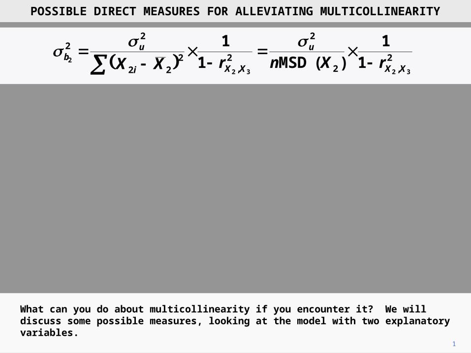
What can you do about multicollinearity if you encounter it? We will discuss some possible measures, looking at the model with two explanatory variables.
2,2
2
2,
222
22
3232
2 11
)(MSD11
XX
u
XXi
ub rXnrXX
2
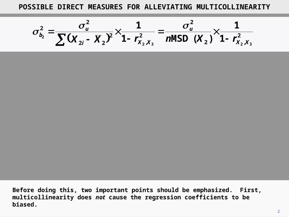
Before doing this, two important points should be emphasized. First, multicollinearity does not cause the regression coefficients to be biased.
POSSIBLE DIRECT MEASURES FOR ALLEVIATING MULTICOLLINEARITY
2,2
2
2,
222
22
3232
2 11
)(MSD11
XX
u
XXi
ub rXnrXX
3
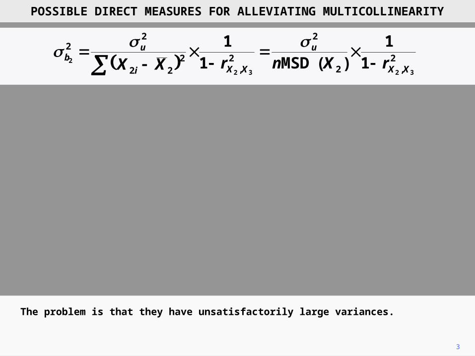
The problem is that they have unsatisfactorily large variances.
POSSIBLE DIRECT MEASURES FOR ALLEVIATING MULTICOLLINEARITY
2,2
2
2,
222
22
3232
2 11
)(MSD11
XX
u
XXi
ub rXnrXX
4
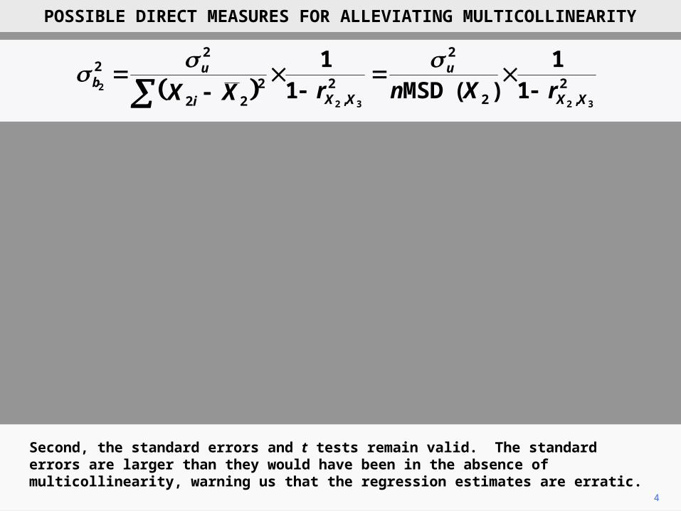
Second, the standard errors and t tests remain valid. The standard errors are larger than they would have been in the absence of multicollinearity, warning us that the regression estimates are erratic.
POSSIBLE DIRECT MEASURES FOR ALLEVIATING MULTICOLLINEARITY
2,2
2
2,
222
22
3232
2 11
)(MSD11
XX
u
XXi
ub rXnrXX
5
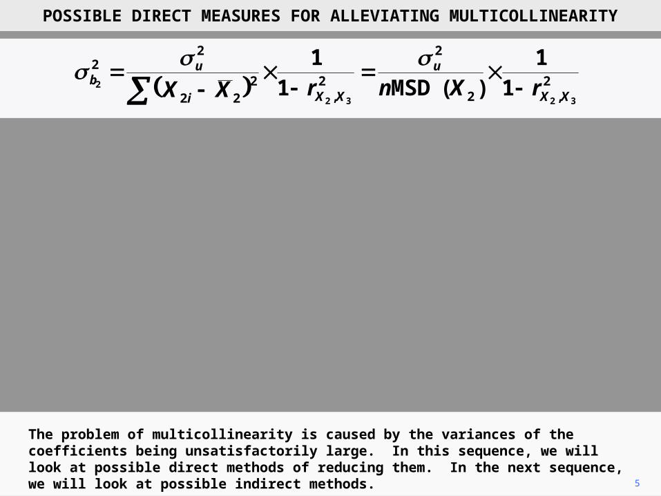
The problem of multicollinearity is caused by the variances of the coefficients being unsatisfactorily large. In this sequence, we will look at possible direct methods of reducing them. In the next sequence, we will look at possible indirect methods.
POSSIBLE DIRECT MEASURES FOR ALLEVIATING MULTICOLLINEARITY
2,2
2
2,
222
22
3232
2 11
)(MSD11
XX
u
XXi
ub rXnrXX
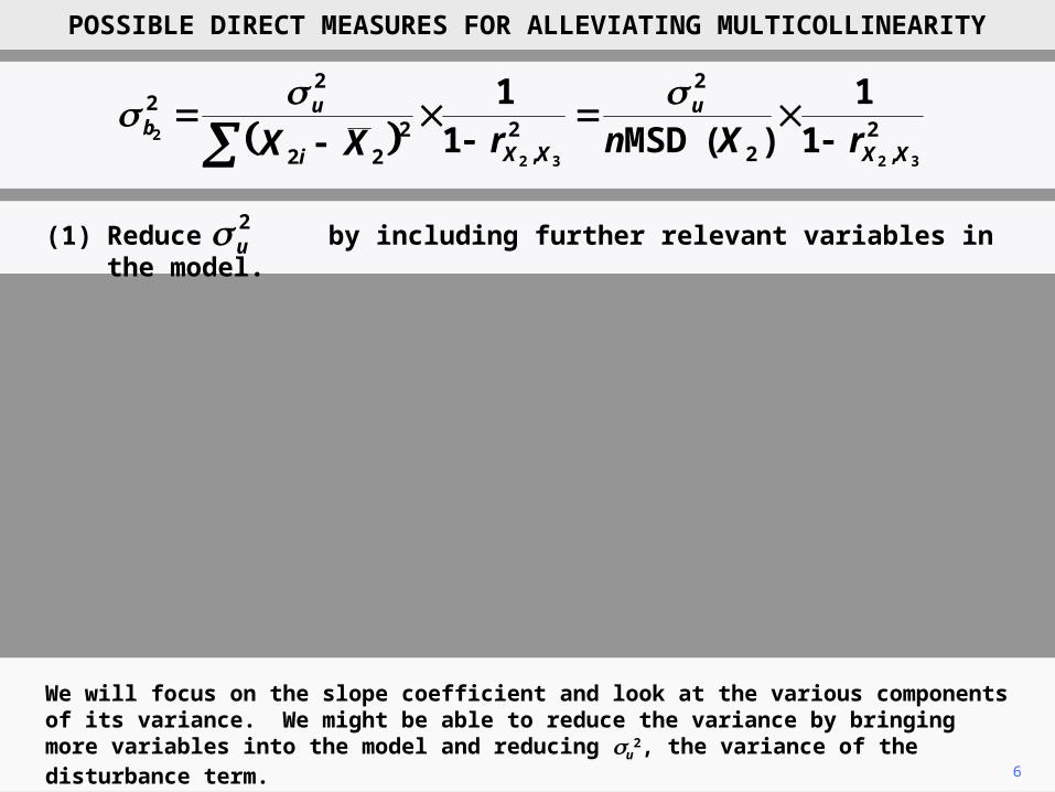
(1) Reduce by including further relevant variables in the model.2u
6
We will focus on the slope coefficient and look at the various components of its variance. We might be able to reduce the variance by bringing more variables into the model and reducing su
2, the variance of the disturbance term.
POSSIBLE DIRECT MEASURES FOR ALLEVIATING MULTICOLLINEARITY
2,2
2
2,
222
22
3232
2 11
)(MSD11
XX
u
XXi
ub rXnrXX
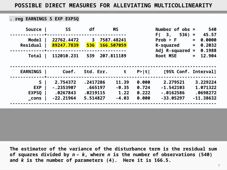
7
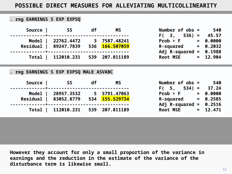
The estimator of the variance of the disturbance term is the residual sum of squares divided by n – k, where n is the number of observations (540) and k is the number of parameters (4). Here it is 166.5.
. reg EARNINGS S EXP EXPSQ
Source | SS df MS Number of obs = 540-------------+------------------------------ F( 3, 536) = 45.57 Model | 22762.4472 3 7587.48241 Prob > F = 0.0000 Residual | 89247.7839 536 166.507059 R-squared = 0.2032-------------+------------------------------ Adj R-squared = 0.1988 Total | 112010.231 539 207.811189 Root MSE = 12.904
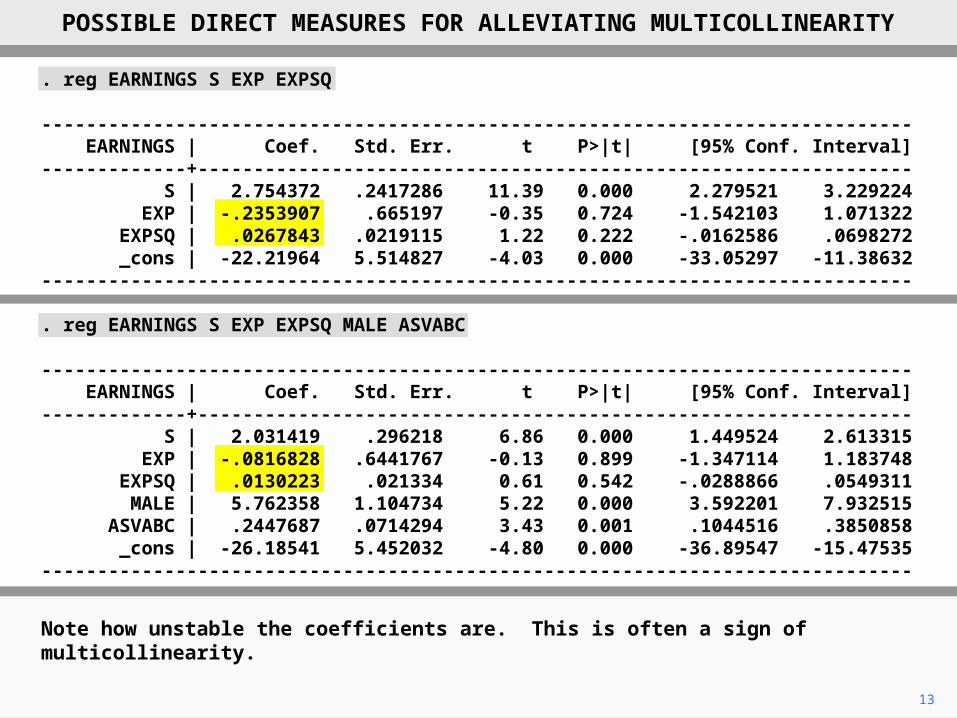
------------------------------------------------------------------------------ EARNINGS | Coef. Std. Err. t P>|t| [95% Conf. Interval]-------------+---------------------------------------------------------------- S | 2.754372 .2417286 11.39 0.000 2.279521 3.229224 EXP | -.2353907 .665197 -0.35 0.724 -1.542103 1.071322 EXPSQ | .0267843 .0219115 1.22 0.222 -.0162586 .0698272 _cons | -22.21964 5.514827 -4.03 0.000 -33.05297 -11.38632------------------------------------------------------------------------------
POSSIBLE DIRECT MEASURES FOR ALLEVIATING MULTICOLLINEARITY
8
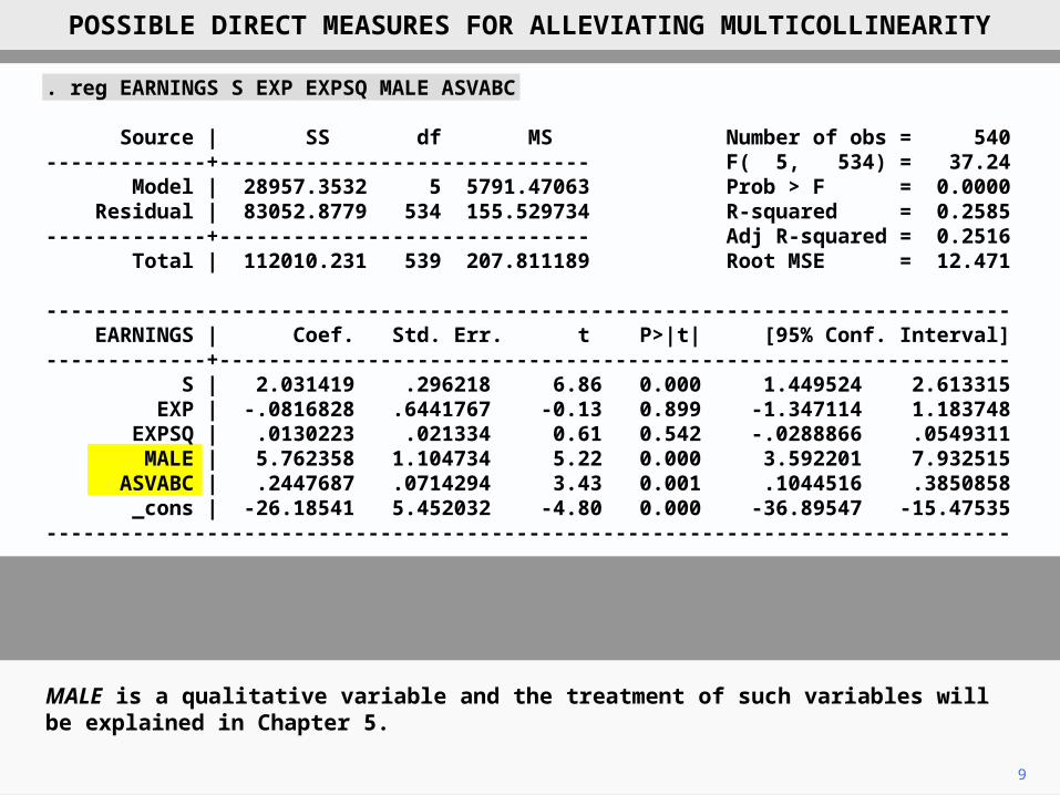
. reg EARNINGS S EXP EXPSQ MALE ASVABC
Source | SS df MS Number of obs = 540-------------+------------------------------ F( 5, 534) = 37.24 Model | 28957.3532 5 5791.47063 Prob > F = 0.0000 Residual | 83052.8779 534 155.529734 R-squared = 0.2585-------------+------------------------------ Adj R-squared = 0.2516 Total | 112010.231 539 207.811189 Root MSE = 12.471
------------------------------------------------------------------------------ EARNINGS | Coef. Std. Err. t P>|t| [95% Conf. Interval]-------------+---------------------------------------------------------------- S | 2.031419 .296218 6.86 0.000 1.449524 2.613315 EXP | -.0816828 .6441767 -0.13 0.899 -1.347114 1.183748 EXPSQ | .0130223 .021334 0.61 0.542 -.0288866 .0549311 MALE | 5.762358 1.104734 5.22 0.000 3.592201 7.932515 ASVABC | .2447687 .0714294 3.43 0.001 .1044516 .3850858 _cons | -26.18541 5.452032 -4.80 0.000 -36.89547 -15.47535------------------------------------------------------------------------------
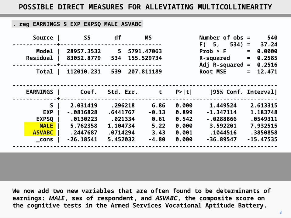
We now add two new variables that are often found to be determinants of earnings: MALE, sex of respondent, and ASVABC, the composite score on the cognitive tests in the Armed Services Vocational Aptitude Battery.
POSSIBLE DIRECT MEASURES FOR ALLEVIATING MULTICOLLINEARITY
9
MALE is a qualitative variable and the treatment of such variables will be explained in Chapter 5.
POSSIBLE DIRECT MEASURES FOR ALLEVIATING MULTICOLLINEARITY
. reg EARNINGS S EXP EXPSQ MALE ASVABC
Source | SS df MS Number of obs = 540-------------+------------------------------ F( 5, 534) = 37.24 Model | 28957.3532 5 5791.47063 Prob > F = 0.0000 Residual | 83052.8779 534 155.529734 R-squared = 0.2585-------------+------------------------------ Adj R-squared = 0.2516 Total | 112010.231 539 207.811189 Root MSE = 12.471
------------------------------------------------------------------------------ EARNINGS | Coef. Std. Err. t P>|t| [95% Conf. Interval]-------------+---------------------------------------------------------------- S | 2.031419 .296218 6.86 0.000 1.449524 2.613315 EXP | -.0816828 .6441767 -0.13 0.899 -1.347114 1.183748 EXPSQ | .0130223 .021334 0.61 0.542 -.0288866 .0549311 MALE | 5.762358 1.104734 5.22 0.000 3.592201 7.932515 ASVABC | .2447687 .0714294 3.43 0.001 .1044516 .3850858 _cons | -26.18541 5.452032 -4.80 0.000 -36.89547 -15.47535------------------------------------------------------------------------------
10
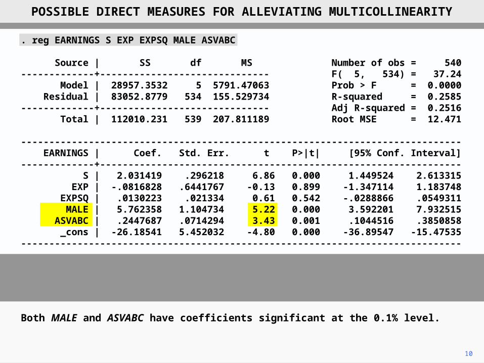
Both MALE and ASVABC have coefficients significant at the 0.1% level.
POSSIBLE DIRECT MEASURES FOR ALLEVIATING MULTICOLLINEARITY
. reg EARNINGS S EXP EXPSQ
Source | SS df MS Number of obs = 540-------------+------------------------------ F( 3, 536) = 45.57 Model | 22762.4472 3 7587.48241 Prob > F = 0.0000 Residual | 89247.7839 536 166.507059 R-squared = 0.2032-------------+------------------------------ Adj R-squared = 0.1988 Total | 112010.231 539 207.811189 Root MSE = 12.904
11
However they account for only a small proportion of the variance in earnings and the reduction in the estimate of the variance of the disturbance term is likewise small.
POSSIBLE DIRECT MEASURES FOR ALLEVIATING MULTICOLLINEARITY
. reg EARNINGS S EXP EXPSQ MALE ASVABC
Source | SS df MS Number of obs = 540-------------+------------------------------ F( 5, 534) = 37.24 Model | 28957.3532 5 5791.47063 Prob > F = 0.0000 Residual | 83052.8779 534 155.529734 R-squared = 0.2585-------------+------------------------------ Adj R-squared = 0.2516 Total | 112010.231 539 207.811189 Root MSE = 12.471
12
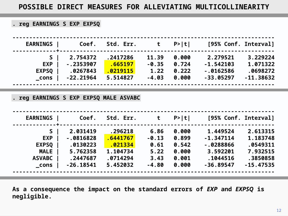
As a consequence the impact on the standard errors of EXP and EXPSQ is negligible.
POSSIBLE DIRECT MEASURES FOR ALLEVIATING MULTICOLLINEARITY
. reg EARNINGS S EXP EXPSQ
------------------------------------------------------------------------------ EARNINGS | Coef. Std. Err. t P>|t| [95% Conf. Interval]-------------+---------------------------------------------------------------- S | 2.754372 .2417286 11.39 0.000 2.279521 3.229224 EXP | -.2353907 .665197 -0.35 0.724 -1.542103 1.071322 EXPSQ | .0267843 .0219115 1.22 0.222 -.0162586 .0698272 _cons | -22.21964 5.514827 -4.03 0.000 -33.05297 -11.38632------------------------------------------------------------------------------
. reg EARNINGS S EXP EXPSQ MALE ASVABC
------------------------------------------------------------------------------ EARNINGS | Coef. Std. Err. t P>|t| [95% Conf. Interval]-------------+---------------------------------------------------------------- S | 2.031419 .296218 6.86 0.000 1.449524 2.613315 EXP | -.0816828 .6441767 -0.13 0.899 -1.347114 1.183748 EXPSQ | .0130223 .021334 0.61 0.542 -.0288866 .0549311 MALE | 5.762358 1.104734 5.22 0.000 3.592201 7.932515 ASVABC | .2447687 .0714294 3.43 0.001 .1044516 .3850858 _cons | -26.18541 5.452032 -4.80 0.000 -36.89547 -15.47535------------------------------------------------------------------------------
13
Note how unstable the coefficients are. This is often a sign of multicollinearity.
POSSIBLE DIRECT MEASURES FOR ALLEVIATING MULTICOLLINEARITY
14
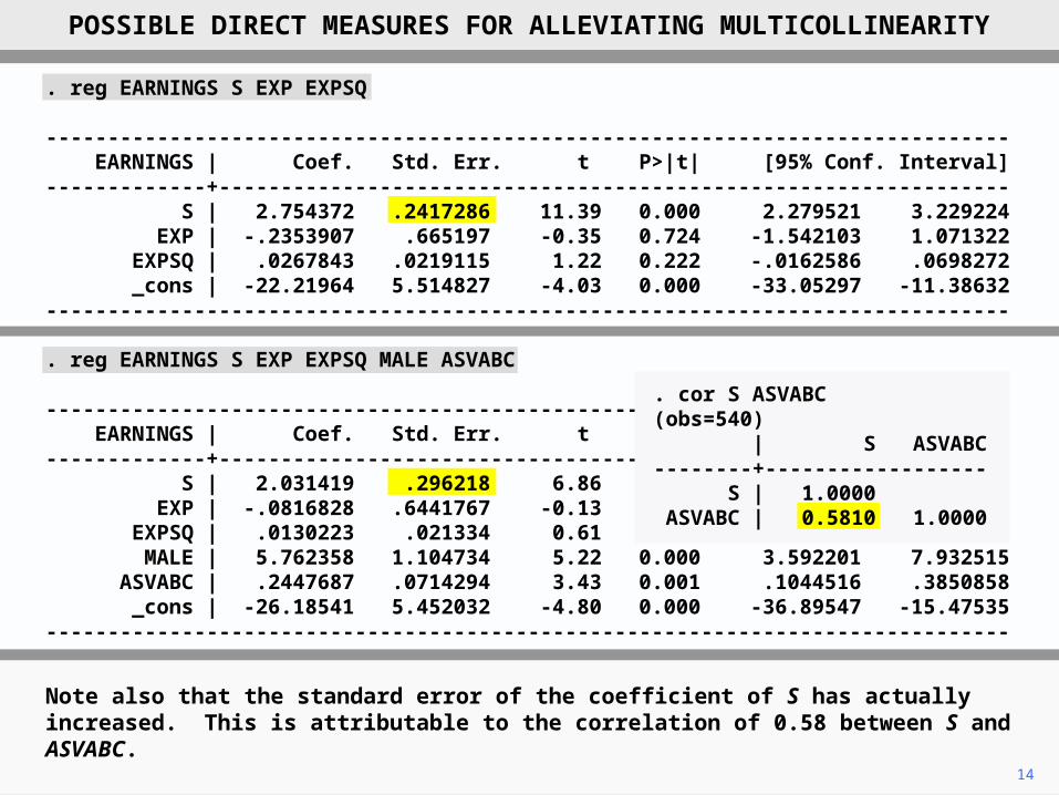
Note also that the standard error of the coefficient of S has actually increased. This is attributable to the correlation of 0.58 between S and ASVABC.
POSSIBLE DIRECT MEASURES FOR ALLEVIATING MULTICOLLINEARITY
. reg EARNINGS S EXP EXPSQ
------------------------------------------------------------------------------ EARNINGS | Coef. Std. Err. t P>|t| [95% Conf. Interval]-------------+---------------------------------------------------------------- S | 2.754372 .2417286 11.39 0.000 2.279521 3.229224 EXP | -.2353907 .665197 -0.35 0.724 -1.542103 1.071322 EXPSQ | .0267843 .0219115 1.22 0.222 -.0162586 .0698272 _cons | -22.21964 5.514827 -4.03 0.000 -33.05297 -11.38632------------------------------------------------------------------------------
. reg EARNINGS S EXP EXPSQ MALE ASVABC
------------------------------------------------------------------------------ EARNINGS | Coef. Std. Err. t P>|t| [95% Conf. Interval]-------------+---------------------------------------------------------------- S | 2.031419 .296218 6.86 0.000 1.449524 2.613315 EXP | -.0816828 .6441767 -0.13 0.899 -1.347114 1.183748 EXPSQ | .0130223 .021334 0.61 0.542 -.0288866 .0549311 MALE | 5.762358 1.104734 5.22 0.000 3.592201 7.932515 ASVABC | .2447687 .0714294 3.43 0.001 .1044516 .3850858 _cons | -26.18541 5.452032 -4.80 0.000 -36.89547 -15.47535------------------------------------------------------------------------------
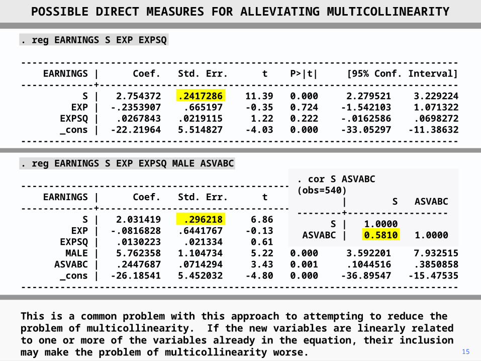
. cor S ASVABC(obs=540) | S ASVABC--------+------------------ S | 1.0000 ASVABC | 0.5810 1.0000
15
This is a common problem with this approach to attempting to reduce the problem of multicollinearity. If the new variables are linearly related to one or more of the variables already in the equation, their inclusion may make the problem of multicollinearity worse.
. reg EARNINGS S EXP EXPSQ
------------------------------------------------------------------------------ EARNINGS | Coef. Std. Err. t P>|t| [95% Conf. Interval]-------------+---------------------------------------------------------------- S | 2.754372 .2417286 11.39 0.000 2.279521 3.229224 EXP | -.2353907 .665197 -0.35 0.724 -1.542103 1.071322 EXPSQ | .0267843 .0219115 1.22 0.222 -.0162586 .0698272 _cons | -22.21964 5.514827 -4.03 0.000 -33.05297 -11.38632------------------------------------------------------------------------------
. reg EARNINGS S EXP EXPSQ MALE ASVABC
------------------------------------------------------------------------------ EARNINGS | Coef. Std. Err. t P>|t| [95% Conf. Interval]-------------+---------------------------------------------------------------- S | 2.031419 .296218 6.86 0.000 1.449524 2.613315 EXP | -.0816828 .6441767 -0.13 0.899 -1.347114 1.183748 EXPSQ | .0130223 .021334 0.61 0.542 -.0288866 .0549311 MALE | 5.762358 1.104734 5.22 0.000 3.592201 7.932515 ASVABC | .2447687 .0714294 3.43 0.001 .1044516 .3850858 _cons | -26.18541 5.452032 -4.80 0.000 -36.89547 -15.47535------------------------------------------------------------------------------
. cor S ASVABC(obs=540) | S ASVABC--------+------------------ S | 1.0000 ASVABC | 0.5810 1.0000
POSSIBLE DIRECT MEASURES FOR ALLEVIATING MULTICOLLINEARITY
16
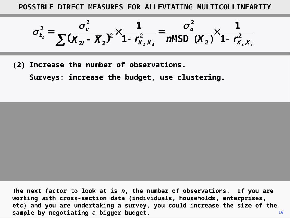
The next factor to look at is n, the number of observations. If you are working with cross-section data (individuals, households, enterprises, etc) and you are undertaking a survey, you could increase the size of the sample by negotiating a bigger budget.
POSSIBLE DIRECT MEASURES FOR ALLEVIATING MULTICOLLINEARITY
2,2
2
2,
222
22
3232
2 11
)(MSD11
XX
u
XXi
ub rXnrXX
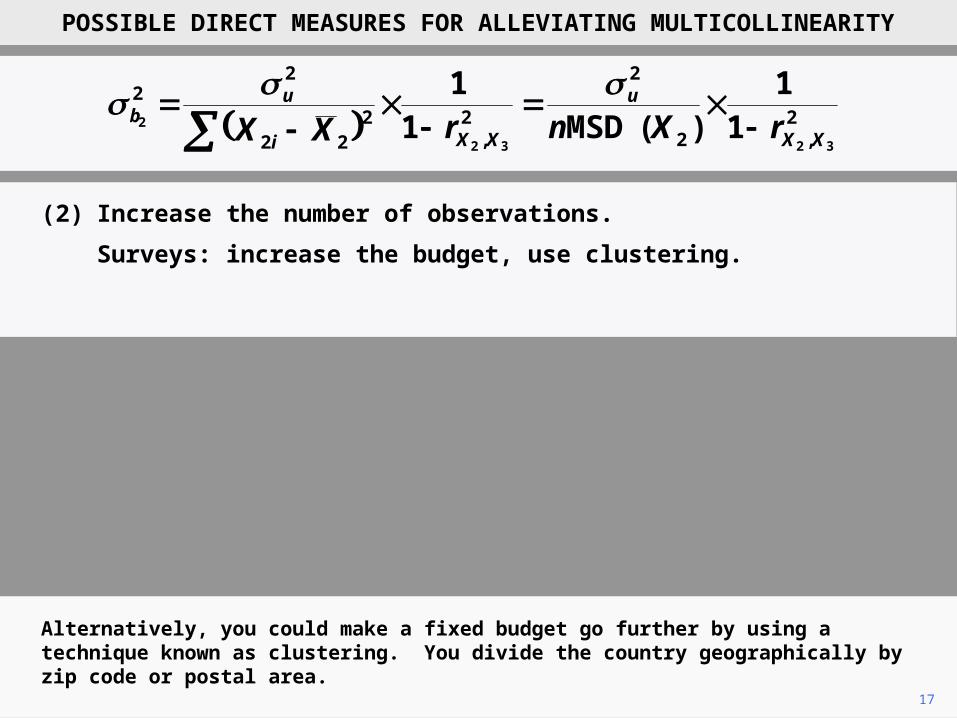
(2) Increase the number of observations.
Surveys: increase the budget, use clustering.
17
Alternatively, you could make a fixed budget go further by using a technique known as clustering. You divide the country geographically by zip code or postal area.
POSSIBLE DIRECT MEASURES FOR ALLEVIATING MULTICOLLINEARITY
2,2
2
2,
222
22
3232
2 11
)(MSD11
XX
u
XXi
ub rXnrXX
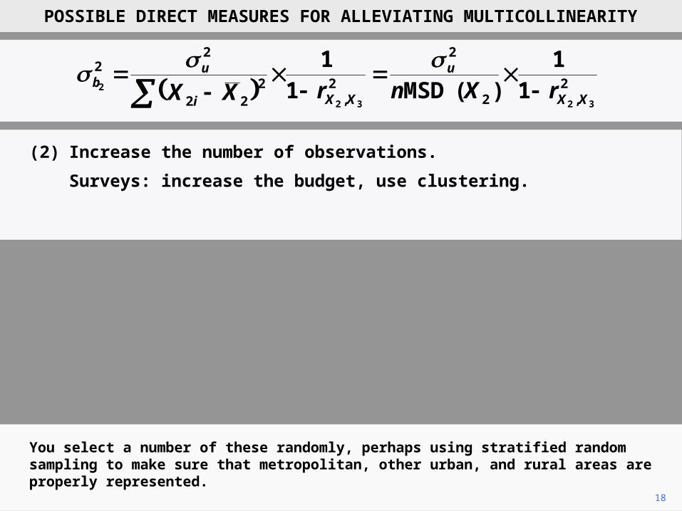
(2) Increase the number of observations.
Surveys: increase the budget, use clustering.
18
You select a number of these randomly, perhaps using stratified random sampling to make sure that metropolitan, other urban, and rural areas are properly represented.
POSSIBLE DIRECT MEASURES FOR ALLEVIATING MULTICOLLINEARITY
2,2
2
2,
222
22
3232
2 11
)(MSD11
XX
u
XXi
ub rXnrXX
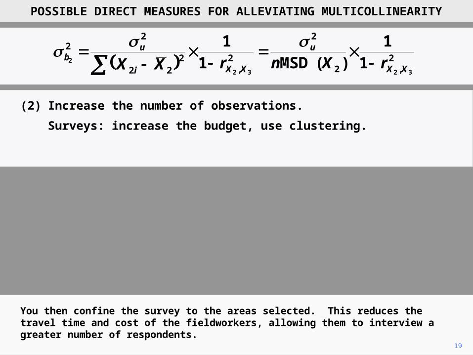
(2) Increase the number of observations.
Surveys: increase the budget, use clustering.
19
You then confine the survey to the areas selected. This reduces the travel time and cost of the fieldworkers, allowing them to interview a greater number of respondents.
POSSIBLE DIRECT MEASURES FOR ALLEVIATING MULTICOLLINEARITY
2,2
2
2,
222
22
3232
2 11
)(MSD11
XX
u
XXi
ub rXnrXX
(2) Increase the number of observations.
Surveys: increase the budget, use clustering.
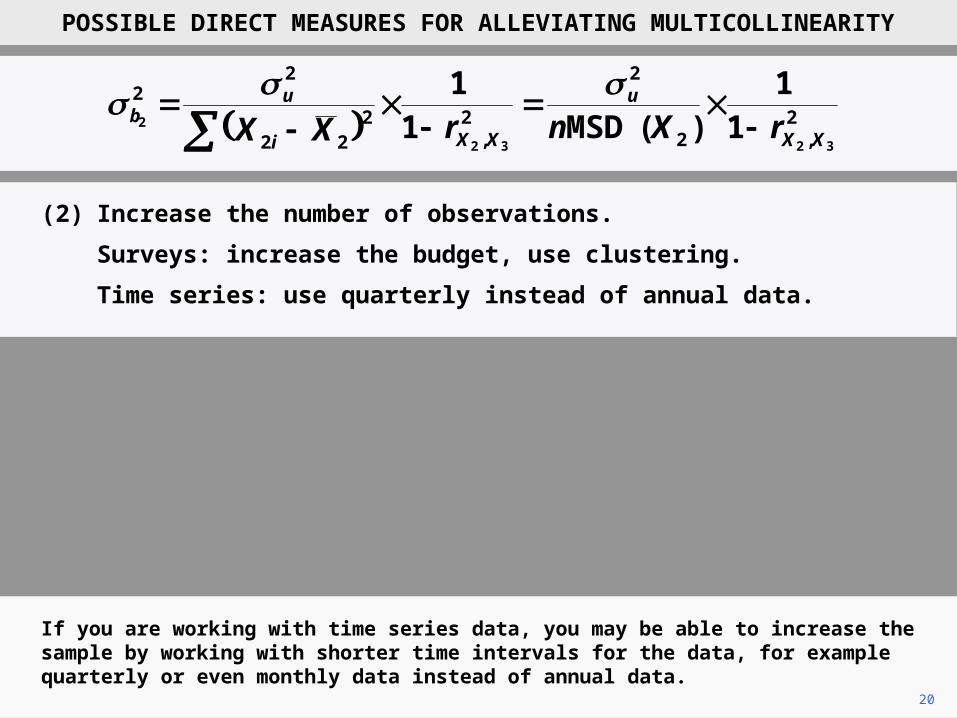
(2) Increase the number of observations.
Surveys: increase the budget, use clustering.
Time series: use quarterly instead of annual data.
20
If you are working with time series data, you may be able to increase the sample by working with shorter time intervals for the data, for example quarterly or even monthly data instead of annual data.
POSSIBLE DIRECT MEASURES FOR ALLEVIATING MULTICOLLINEARITY
2,2
2
2,
222
22
3232
2 11
)(MSD11
XX
u
XXi
ub rXnrXX
. reg EARNINGS S EXP EXPSQ MALE ASVABC
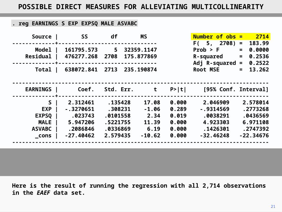
Source | SS df MS Number of obs = 2714-------------+------------------------------ F( 5, 2708) = 183.99 Model | 161795.573 5 32359.1147 Prob > F = 0.0000 Residual | 476277.268 2708 175.877869 R-squared = 0.2536-------------+------------------------------ Adj R-squared = 0.2522 Total | 638072.841 2713 235.190874 Root MSE = 13.262
------------------------------------------------------------------------------ EARNINGS | Coef. Std. Err. t P>|t| [95% Conf. Interval]-------------+---------------------------------------------------------------- S | 2.312461 .135428 17.08 0.000 2.046909 2.578014 EXP | -.3270651 .308231 -1.06 0.289 -.9314569 .2773268 EXPSQ | .023743 .0101558 2.34 0.019 .0038291 .0436569 MALE | 5.947206 .5221755 11.39 0.000 4.923303 6.971108 ASVABC | .2086846 .0336869 6.19 0.000 .1426301 .2747392 _cons | -27.40462 2.579435 -10.62 0.000 -32.46248 -22.34676------------------------------------------------------------------------------
21
Here is the result of running the regression with all 2,714 observations in the EAEF data set.
POSSIBLE DIRECT MEASURES FOR ALLEVIATING MULTICOLLINEARITY
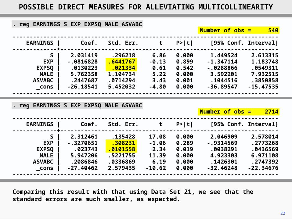
. reg EARNINGS S EXP EXPSQ MALE ASVABC Number of obs = 540------------------------------------------------------------------------------ EARNINGS | Coef. Std. Err. t P>|t| [95% Conf. Interval]-------------+---------------------------------------------------------------- S | 2.031419 .296218 6.86 0.000 1.449524 2.613315 EXP | -.0816828 .6441767 -0.13 0.899 -1.347114 1.183748 EXPSQ | .0130223 .021334 0.61 0.542 -.0288866 .0549311 MALE | 5.762358 1.104734 5.22 0.000 3.592201 7.932515 ASVABC | .2447687 .0714294 3.43 0.001 .1044516 .3850858 _cons | -26.18541 5.452032 -4.80 0.000 -36.89547 -15.47535------------------------------------------------------------------------------
. reg EARNINGS S EXP EXPSQ MALE ASVABC Number of obs = 2714------------------------------------------------------------------------------ EARNINGS | Coef. Std. Err. t P>|t| [95% Conf. Interval]-------------+---------------------------------------------------------------- S | 2.312461 .135428 17.08 0.000 2.046909 2.578014 EXP | -.3270651 .308231 -1.06 0.289 -.9314569 .2773268 EXPSQ | .023743 .0101558 2.34 0.019 .0038291 .0436569 MALE | 5.947206 .5221755 11.39 0.000 4.923303 6.971108 ASVABC | .2086846 .0336869 6.19 0.000 .1426301 .2747392 _cons | -27.40462 2.579435 -10.62 0.000 -32.46248 -22.34676------------------------------------------------------------------------------
22
Comparing this result with that using Data Set 21, we see that the standard errors are much smaller, as expected.
POSSIBLE DIRECT MEASURES FOR ALLEVIATING MULTICOLLINEARITY
23
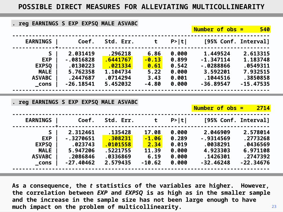
As a consequence, the t statistics of the variables are higher. However, the correlation between EXP and EXPSQ is as high as in the smaller sample and the increase in the sample size has not been large enough to have much impact on the problem of multicollinearity.
. reg EARNINGS S EXP EXPSQ MALE ASVABC Number of obs = 540------------------------------------------------------------------------------ EARNINGS | Coef. Std. Err. t P>|t| [95% Conf. Interval]-------------+---------------------------------------------------------------- S | 2.031419 .296218 6.86 0.000 1.449524 2.613315 EXP | -.0816828 .6441767 -0.13 0.899 -1.347114 1.183748 EXPSQ | .0130223 .021334 0.61 0.542 -.0288866 .0549311 MALE | 5.762358 1.104734 5.22 0.000 3.592201 7.932515 ASVABC | .2447687 .0714294 3.43 0.001 .1044516 .3850858 _cons | -26.18541 5.452032 -4.80 0.000 -36.89547 -15.47535------------------------------------------------------------------------------
. reg EARNINGS S EXP EXPSQ MALE ASVABC Number of obs = 2714------------------------------------------------------------------------------ EARNINGS | Coef. Std. Err. t P>|t| [95% Conf. Interval]-------------+---------------------------------------------------------------- S | 2.312461 .135428 17.08 0.000 2.046909 2.578014 EXP | -.3270651 .308231 -1.06 0.289 -.9314569 .2773268 EXPSQ | .023743 .0101558 2.34 0.019 .0038291 .0436569 MALE | 5.947206 .5221755 11.39 0.000 4.923303 6.971108 ASVABC | .2086846 .0336869 6.19 0.000 .1426301 .2747392 _cons | -27.40462 2.579435 -10.62 0.000 -32.46248 -22.34676------------------------------------------------------------------------------
POSSIBLE DIRECT MEASURES FOR ALLEVIATING MULTICOLLINEARITY
24
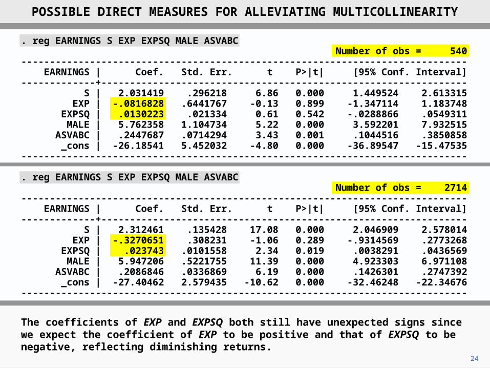
The coefficients of EXP and EXPSQ both still have unexpected signs since we expect the coefficient of EXP to be positive and that of EXPSQ to be negative, reflecting diminishing returns.
. reg EARNINGS S EXP EXPSQ MALE ASVABC Number of obs = 540------------------------------------------------------------------------------ EARNINGS | Coef. Std. Err. t P>|t| [95% Conf. Interval]-------------+---------------------------------------------------------------- S | 2.031419 .296218 6.86 0.000 1.449524 2.613315 EXP | -.0816828 .6441767 -0.13 0.899 -1.347114 1.183748 EXPSQ | .0130223 .021334 0.61 0.542 -.0288866 .0549311 MALE | 5.762358 1.104734 5.22 0.000 3.592201 7.932515 ASVABC | .2447687 .0714294 3.43 0.001 .1044516 .3850858 _cons | -26.18541 5.452032 -4.80 0.000 -36.89547 -15.47535------------------------------------------------------------------------------
. reg EARNINGS S EXP EXPSQ MALE ASVABC Number of obs = 2714------------------------------------------------------------------------------ EARNINGS | Coef. Std. Err. t P>|t| [95% Conf. Interval]-------------+---------------------------------------------------------------- S | 2.312461 .135428 17.08 0.000 2.046909 2.578014 EXP | -.3270651 .308231 -1.06 0.289 -.9314569 .2773268 EXPSQ | .023743 .0101558 2.34 0.019 .0038291 .0436569 MALE | 5.947206 .5221755 11.39 0.000 4.923303 6.971108 ASVABC | .2086846 .0336869 6.19 0.000 .1426301 .2747392 _cons | -27.40462 2.579435 -10.62 0.000 -32.46248 -22.34676------------------------------------------------------------------------------
POSSIBLE DIRECT MEASURES FOR ALLEVIATING MULTICOLLINEARITY
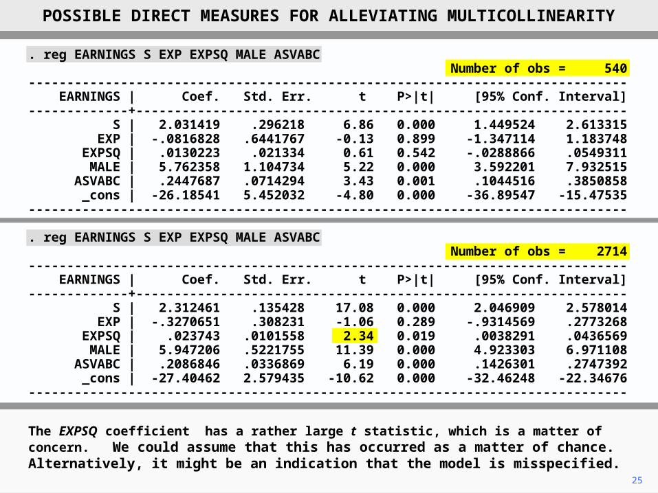
25
The EXPSQ coefficient has a rather large t statistic, which is a matter of concern. We could assume that this has occurred as a matter of chance. Alternatively, it might be an indication that the model is misspecified.
. reg EARNINGS S EXP EXPSQ MALE ASVABC Number of obs = 540------------------------------------------------------------------------------ EARNINGS | Coef. Std. Err. t P>|t| [95% Conf. Interval]-------------+---------------------------------------------------------------- S | 2.031419 .296218 6.86 0.000 1.449524 2.613315 EXP | -.0816828 .6441767 -0.13 0.899 -1.347114 1.183748 EXPSQ | .0130223 .021334 0.61 0.542 -.0288866 .0549311 MALE | 5.762358 1.104734 5.22 0.000 3.592201 7.932515 ASVABC | .2447687 .0714294 3.43 0.001 .1044516 .3850858 _cons | -26.18541 5.452032 -4.80 0.000 -36.89547 -15.47535------------------------------------------------------------------------------
. reg EARNINGS S EXP EXPSQ MALE ASVABC Number of obs = 2714------------------------------------------------------------------------------ EARNINGS | Coef. Std. Err. t P>|t| [95% Conf. Interval]-------------+---------------------------------------------------------------- S | 2.312461 .135428 17.08 0.000 2.046909 2.578014 EXP | -.3270651 .308231 -1.06 0.289 -.9314569 .2773268 EXPSQ | .023743 .0101558 2.34 0.019 .0038291 .0436569 MALE | 5.947206 .5221755 11.39 0.000 4.923303 6.971108 ASVABC | .2086846 .0336869 6.19 0.000 .1426301 .2747392 _cons | -27.40462 2.579435 -10.62 0.000 -32.46248 -22.34676------------------------------------------------------------------------------
POSSIBLE DIRECT MEASURES FOR ALLEVIATING MULTICOLLINEARITY
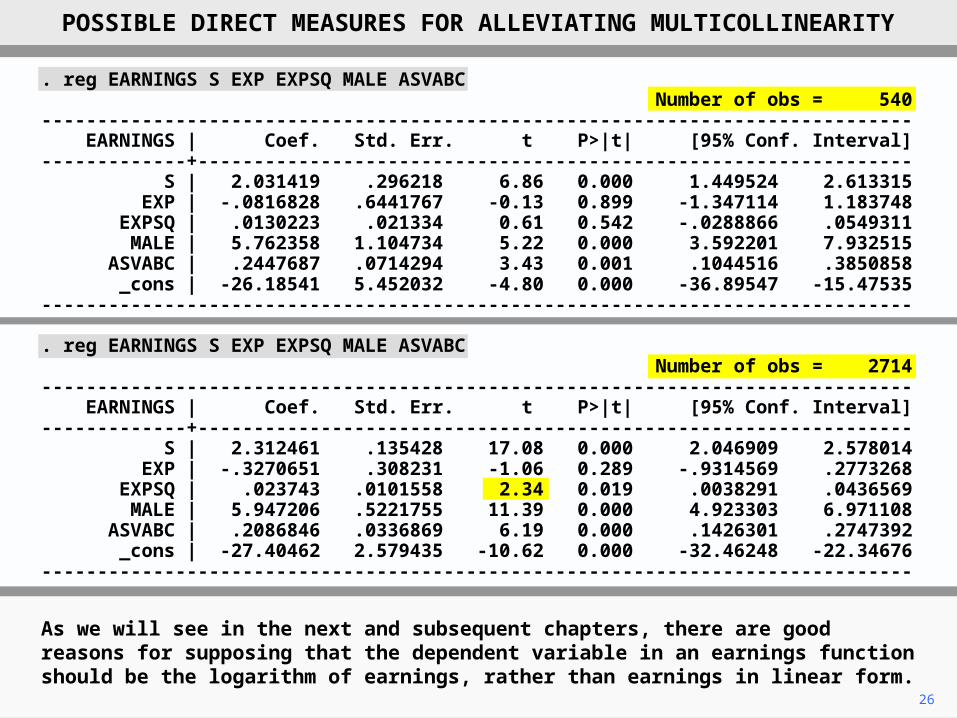
26
As we will see in the next and subsequent chapters, there are good reasons for supposing that the dependent variable in an earnings function should be the logarithm of earnings, rather than earnings in linear form.
. reg EARNINGS S EXP EXPSQ MALE ASVABC Number of obs = 540------------------------------------------------------------------------------ EARNINGS | Coef. Std. Err. t P>|t| [95% Conf. Interval]-------------+---------------------------------------------------------------- S | 2.031419 .296218 6.86 0.000 1.449524 2.613315 EXP | -.0816828 .6441767 -0.13 0.899 -1.347114 1.183748 EXPSQ | .0130223 .021334 0.61 0.542 -.0288866 .0549311 MALE | 5.762358 1.104734 5.22 0.000 3.592201 7.932515 ASVABC | .2447687 .0714294 3.43 0.001 .1044516 .3850858 _cons | -26.18541 5.452032 -4.80 0.000 -36.89547 -15.47535------------------------------------------------------------------------------
. reg EARNINGS S EXP EXPSQ MALE ASVABC Number of obs = 2714------------------------------------------------------------------------------ EARNINGS | Coef. Std. Err. t P>|t| [95% Conf. Interval]-------------+---------------------------------------------------------------- S | 2.312461 .135428 17.08 0.000 2.046909 2.578014 EXP | -.3270651 .308231 -1.06 0.289 -.9314569 .2773268 EXPSQ | .023743 .0101558 2.34 0.019 .0038291 .0436569 MALE | 5.947206 .5221755 11.39 0.000 4.923303 6.971108 ASVABC | .2086846 .0336869 6.19 0.000 .1426301 .2747392 _cons | -27.40462 2.579435 -10.62 0.000 -32.46248 -22.34676------------------------------------------------------------------------------
POSSIBLE DIRECT MEASURES FOR ALLEVIATING MULTICOLLINEARITY
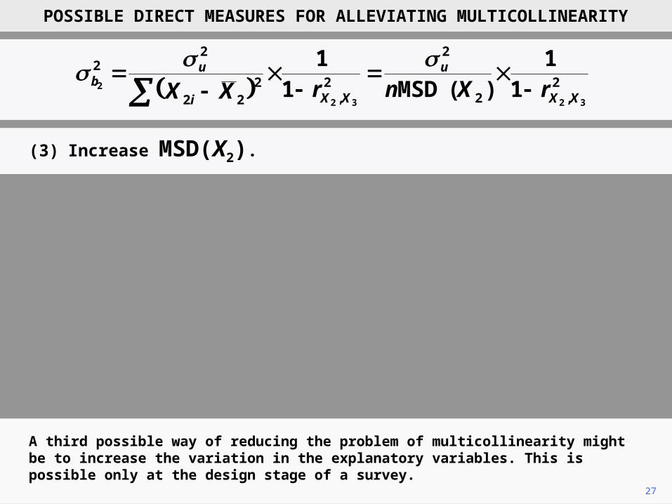
27
A third possible way of reducing the problem of multicollinearity might be to increase the variation in the explanatory variables. This is possible only at the design stage of a survey.
(3) Increase MSD(X2).
POSSIBLE DIRECT MEASURES FOR ALLEVIATING MULTICOLLINEARITY
2,2
2
2,
222
22
3232
2 11
)(MSD11
XX
u
XXi
ub rXnrXX
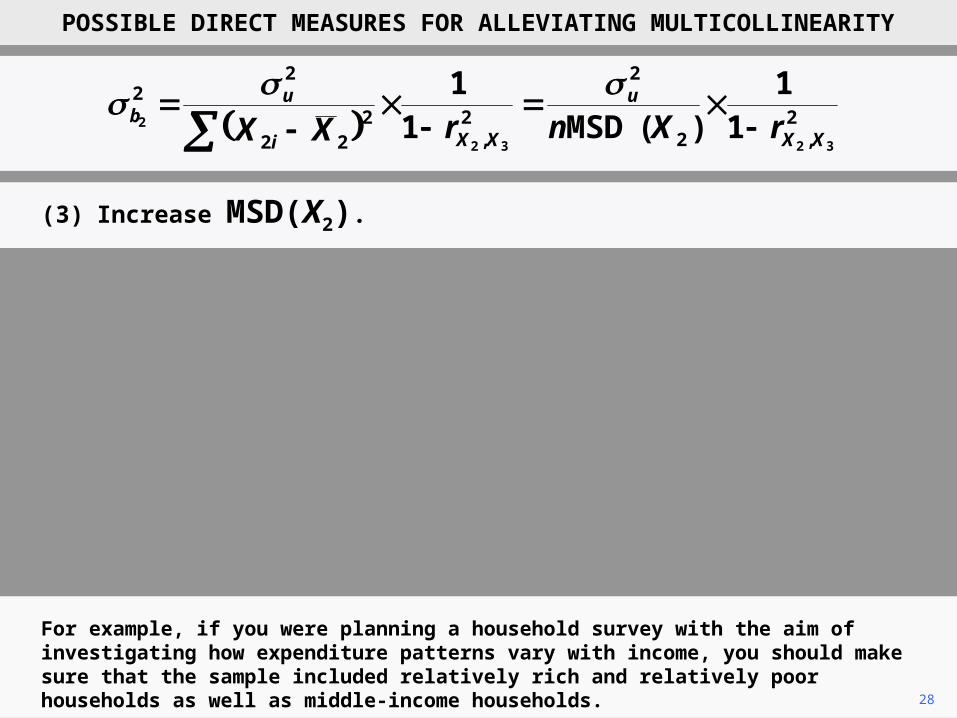
28
For example, if you were planning a household survey with the aim of investigating how expenditure patterns vary with income, you should make sure that the sample included relatively rich and relatively poor households as well as middle-income households.
POSSIBLE DIRECT MEASURES FOR ALLEVIATING MULTICOLLINEARITY
2,2
2
2,
222
22
3232
2 11
)(MSD11
XX
u
XXi
ub rXnrXX
(3) Increase MSD(X2).
32 ,XXr
29
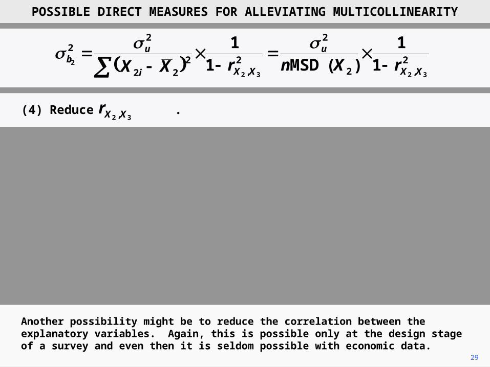
Another possibility might be to reduce the correlation between the explanatory variables. Again, this is possible only at the design stage of a survey and even then it is seldom possible with economic data.
POSSIBLE DIRECT MEASURES FOR ALLEVIATING MULTICOLLINEARITY
2,2
2
2,
222
22
3232
2 11
)(MSD11
XX
u
XXi
ub rXnrXX
(4) Reduce .
Copyright Christopher Dougherty 2012.
These slideshows may be downloaded by anyone, anywhere for personal use.
Subject to respect for copyright and, where appropriate, attribution, they may be
used as a resource for teaching an econometrics course. There is no need to
refer to the author.
The content of this slideshow comes from Section 3.4 of C. Dougherty,
Introduction to Econometrics, fourth edition 2011, Oxford University Press.
Additional (free) resources for both students and instructors may be
downloaded from the OUP Online Resource Centre
http://www.oup.com/uk/orc/bin/9780199567089/.
Individuals studying econometrics on their own who feel that they might benefit
from participation in a formal course should consider the London School of
Economics summer school course
EC212 Introduction to Econometrics
http://www2.lse.ac.uk/study/summerSchools/summerSchool/Home.aspx
or the University of London International Programmes distance learning course
EC2020 Elements of Econometrics
www.londoninternational.ac.uk/lse.
2012.10.28