positive cell-centered finite volume discretization …positive cell-centered finite volume...

ELSEVIER Applied Numerical Mathematics 16 (1995) 417-438 MATHEMATICS

Positive cell-centered finite volume discretization methods for hyperbolic equations on irregular meshes

M. Berzins *, J.M. Ware

School of Computer Studies, University of Leeds, Leeds LS2 9JT, UK

Abstract

The conditions sufficient to ensure positivity and linearity preservation for a cell-centered finite volume scheme for time-dependent hyperbolic equations using irregular one-dimensional and triangular two-dimensional meshes are derived. The conditions require standard flux limiters to be modified and also involve possible constraints on the meshes. The accuracy of this finite volume scheme is considered and is illustrated by two simple numerical examples.

1. Introduction

An important t rend in numerical methods for the spatial discretization of partial differential equations is the move towards using finite element and finite volume methods on unstructured triangular or tetrahedral meshes. The reasoning underlying this trend is that such methods offer one way of solving problems adaptively on general geometries. The finite volume methods used may be split into cell-vertex methods (in which the solution values are posit ioned at mesh points) and cell-centered methods (in which the solution variables are posit ioned at the centroids of triangles). Cell-vertex methods have a clear advantage over cell-centered methods in that there are fewer unknowns for a given mesh, but a possible disadvantage is that the area (or volume) of each cell is larger. While both methods have their advocates what is clear is that both classes of methods need to be well-understood. In this respect more work has been done on the analysis and derivation of cell-vertex schemes, e.g. see Barth [1], Struijs et al. [17] and van Leer [18] and the references therein. One of the early papers to make an important advance in this area was that of Cockburn et al. [7] which proves a maximum principle for a discontinuous Galerkin method of order k + 1 which may be interpreted as a finite volume type scheme.

In the area of cell-centered schemes on triangles perhaps the first extension of successful one-dimensional schemes to triangles was that of Venkatakrishnan and Barth [19]. Subsequent

* Corresponding author.

0168-9274/95/$09.50 © 1995 Elsevier Science B.V. All rights reserved SSDI 0168-9274(95)00007-0

418 M. Berzins, J.M. Ware/Applied Numerical Mathematics 16 (1995) 417-438

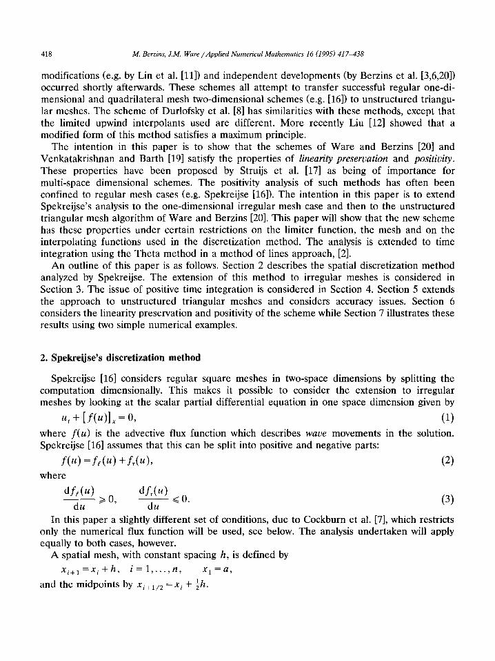
modifications (e.g. by Lin et al. [11]) and independent developments (by Berzins et al. [3,6,20]) occurred shortly afterwards. These schemes all attempt to transfer successful regular one-dimensional and quadrilateral mesh two-dimensional schemes (e.g. [16]) to unstructured triangular meshes. The scheme of Durlofsky et al. [8] has similarities with these methods, except that the limited upwind interpolants used are different. More recently Liu [12] showed that a modified form of this method satisfies a maximum principle.

The intention in this paper is to show that the schemes of Ware and Berzins [20] and Venkatakrishnan and Barth [19] satisfy the properties of linearity preservation and positivity. These properties have been proposed by Struijs et al. [17] as being of importance for multi-space dimensional schemes. The positivity analysis of such methods has often been confined to regular mesh cases (e.g. Spekreijse [16]). The intention in this paper is to extend Spekreijse's analysis to the one-dimensional irregular mesh case and then to the unstructured triangular mesh algorithm of Ware and Berzins [20]. This paper will show that the new scheme has these properties under certain restrictions on the limiter function, the mesh and on the interpolating functions used in the discretization method. The analysis is extended to time integration using the Theta method in a method of lines approach, [2].

An outline of this paper is as follows. Section 2 describes the spatial discretization method analyzed by Spekreijse. The extension of this method to irregular meshes is considered in Section 3. The issue of positive time integration is considered in Section 4. Section 5 extends the approach to unstructured triangular meshes and considers accuracy issues. Section 6 considers the linearity preservation and positivity of the scheme while Section 7 illustrates these results using two simple numerical examples.

2. Spekreijse's discretization method

Spekreijse [16] considers regular square meshes in two-space dimensions by splitting the computation dimensionally. This makes it possible to consider the extension to irregular meshes by looking at the scalar partial differential equation in one space dimension given by

u , + [ f ( U ) ] x = O , (1)

where f ( u ) is the advective flux function which describes wave movements in the solution. Spekreijse [16] assumes that this can be split into positive and negative parts:

f(u)=L(u)+L(u), (2) where

d f t ( u ) dfr(U) d----U-- >~ 0, d---~ ~< 0. (3)

In this paper a slightly different set of conditions, due to Cockburn et al. [7], which restricts only the numerical flux function will be used, see below. The analysis undertaken will apply equally to both cases, however.

A spatial mesh, with constant spacing h, is defined by

Xi+l =Xi + h, i = 1 . . . . , n , xl =a , 1 and the midpoints by Xg+l/2 = x i + gh.

M. Berzins, J,M. Ware/Applied Numerical Mathematics 16 (1995) 417-438 419

Denote by Ui(t) the solution value U(x i, t) at the meshpoint x i at time t. Throughout the paper it will be assumed that all solution values, derivatives and fluxes depend on the time t. The semi-discrete form of (1) is

aG L+l /2 - -L-1 /2 - - + = 0 , (4) at h

where fi+1/2 and f i -1 /2 are the fluxes at the midpoints Xi+l/2 and Xi_a/2 respectively. Spekreijse's method [16]makes use of an approximate Riemann solver such as the well-known Roe or Osher solvers to calculate these fluxes. The flux calculated by this approximate Riemann solver will be defined as

t' r fRm(U/+ 1/2, U/+ 1/2) (5)

and, following Cockburn et al. [7], is assumed to satisfy:

• fRm(U, U ) = f ( u ) ; • fRm(U, V) is nondecreasing in u and nonincreasing in v; • fRm(' , " ) is Lipschitz; • fRm(U, U)= --fRm(g, U).

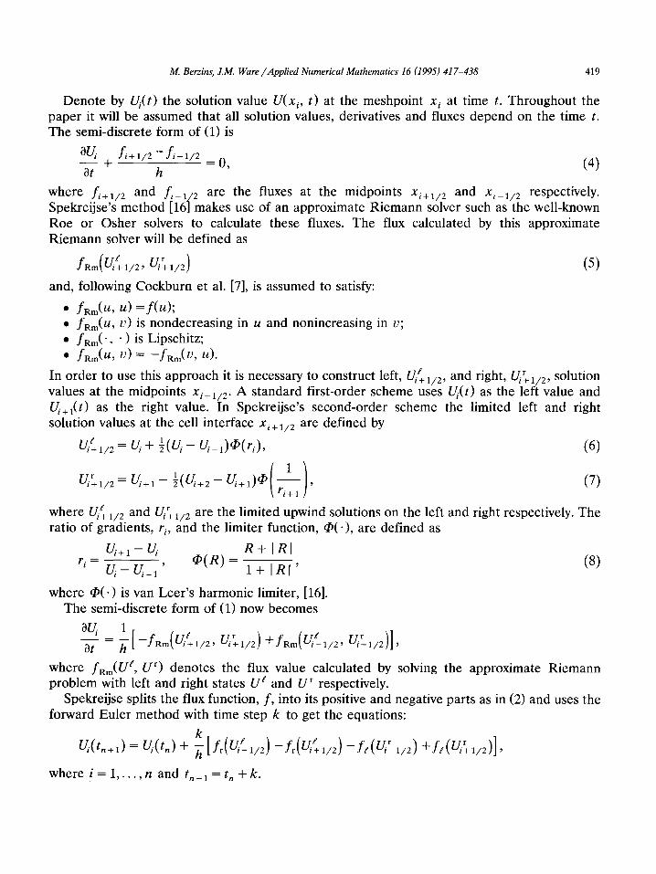
In order to use this approach it is necessary to construct left, Uie+ 1/2, and right, U/+ 1/2, solution values at the midpoints Xi+l/2. A standard first-order scheme uses Ui(t) as the left value and Ui+l(t) as the right value. In Spekreijse's second-order scheme the limited left and right solution values at the cell interface xi+ 1/2 are defined by

1 Vtf+l/2 = U/+ 2 ( U i - U/_l)@(ri) , (6) (1)

- 2 ( ,+2 <+1) @ (7) u r = Ui+l 1 U~ - i + 1/2

where g r G+1/2 and G+1/2 are the limited upwind solutions on the left and right respectively. The ratio of gradients, r i, and the limiter function, @(-), are defined as

U,.+I - U i R + IRI = , @ ( R ) = ( s )

ri U / - U/_ 1 1- -{- IR[ '

where @(.) is van Leer's harmonic limiter, [16]. The semi-discrete form of (1) now becomes

a G. 1 at -- h [--fRm(<f+l/2 ' G+1/2) +fRm(g/f-1/2, G r l / 2 ) ] ,

where fRm(U e, U r) denotes the flux value calculated by solving the approximate Riemann problem with left and right states U e and U r respectively.

Spekreijse splits the flux function, f , into its positive and negative parts as in (2) and uses the forward Euler method with time step k to get the equations:

k U i ( t n + l ) = Ui ( tn ) + ~ - [ f r ( U / / - 1 / 2 ) - - f r ( U / / + l / 2 ) - f l ( u i r - 1 / 2 ) + f l ( U i + l / 2 ) ] ,

where i = 1 . . . . , n and t n+ 1 -D- tn + k.


3. One.dimensional variable mesh formulation

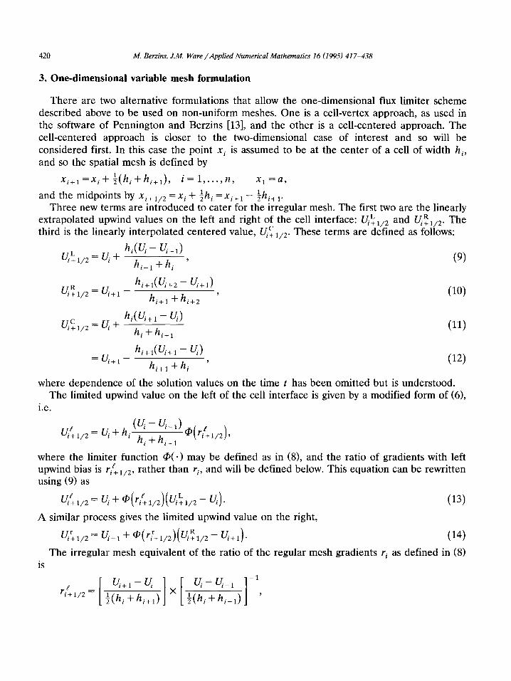
There are two alternative formulat ions that allow the one-dimensional flux limiter scheme described above to be used on non-uni form meshes. One is a cell-vertex approach, as used in the software of Penning ton and Berzins [13], and the o ther is a cell-centered approach. The cell-centered approach is closer to the two-dimensional case of interest and so will be considered first. In this case the point x/ is assumed to be at the center of a cell of width h/, and so the spatial mesh is def ined by

1 Xi+ 1 :X i 'q - -~(hi-Fhi+l), i = 1 . . . . , n , x 1 = a ,

1 1 and the midpoints by x/+1/2 = x i + 2h i = x i + 1 - -~hi+ 1. Three new terms are in t roduced to cater for the irregular mesh. The first two are the linearly

extrapolated upwind values on the left and right of the cell interface: E+I/2L and uRi+I/2. The third is the linearly interpolated centered value, c E+l /2 . These terms are def ined as follows:

h i ( U i - Ui_l) L = (9)

U,,+1/2 U/+ h i - 1 + h i ,

hi+l(U/+2 - U/+I) n = _ (10)

E + l / 2 E'+I hi+l +h i+ 2 ,

hi(U/+ 1 -- U/) c = (11)

E+1/2 E -F h i -F hi+ 1

hi+l(U/+ 1 - U/) = E ' + I - - ' (12)

hi+ 1 + h i

where dependence of the solution values on the t ime t has been omi t ted but is unders tood. The l imited upwind value on the left of the cell interface is given by a modif ied form of (6),

i.e.

f ( E -- U/ - I ) E + I / 2 = Ui + hi h i + h i _ 1 c1)(rf+l/2) '

where the limiter function q)(.) may be def ined as in (8), and the ratio of gradients with left upwind bias is rie+l/2, ra ther than ri, and will be def ined below. This equat ion can be rewrit ten using (9) as

Eg+I/2 = E "~ Cl)(rf+ 1 / 2 ) ( E L I / 2 - E ) " (13)

A similar process gives the l imited upwind value on the right, r R

E'+ 1/2----- Ui+a --I- (/)(r[+ 1/2)(U/+ 1 / 2 - U/+ 1).

is

(14)

The irregular mesh equivalent of the ratio of the regular mesh gradients r i as def ined in (8)

r i + l / 2 = 1 . . . . X 2 ( h i -[- h i + 1) 1 (-h- i~-~-/- 1 )

M. Berzins, J.M. Ware/Applied Numerical Mathematics 16 (1995) 417-438

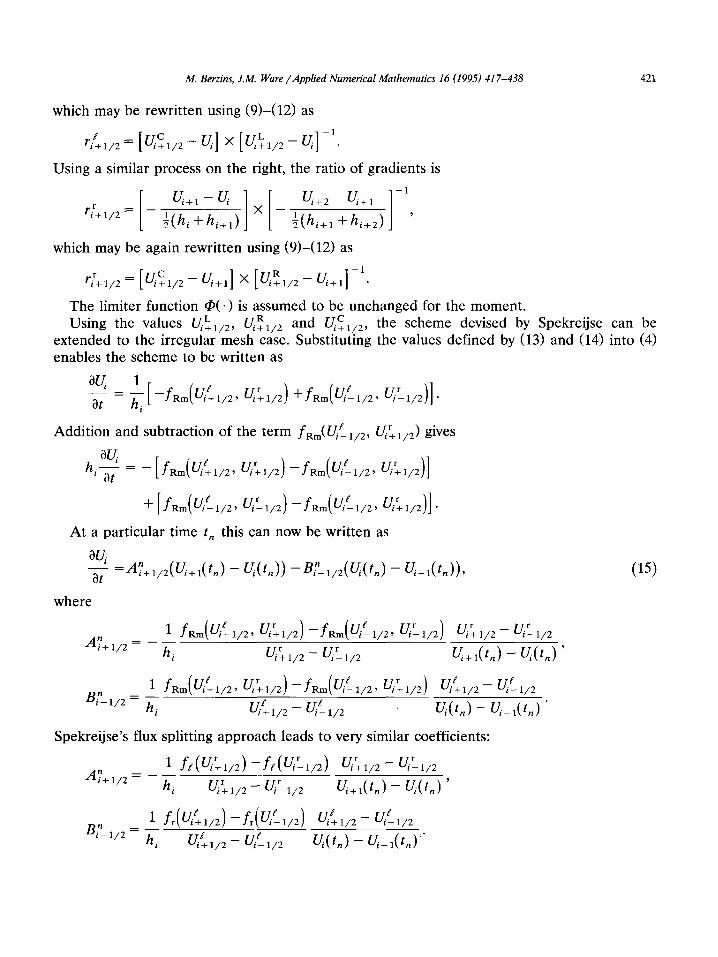
which may be rewritten using (9)-(12) as

C L ¢' .~_ [Ui+ l /2_ U/] x [< .+1/2_ U/] -1 Fi + 1/2

Using a similar process on the right, the ratio of gradients is

[ [ ,+2 +1]1 r ir+l/2 = -- 1 . . . . X -- 1 . . . . '

~ ( h i + h i + , ) 2 ( h i + l + h i + 2 )

421

Spekreijse's flux splitting approach leads to very similar coefficients:

r u r r __ U r 1 f e ( U i + l / e ) - f e ( i - 1 / 2 ) U/+1/2 i-I/2

A7+1/2 - h i U/+ 1 / 2 - ori-1/2 Ui+l(tn) - U/(tn) '

Uf _ e 1 f r ( U i g + l / 2 ) - f r ( / - 1 / 2 ) ' U/- i/2 U/+ 1/2 Bin_l~2 - h i U/t+l/2- U/{_l/2 U i ( t n ) - U/_l(in):"

e r U e r 1 fnm(U~+~/2, U/+1/2)-fnm( i - ~ / 2 , U~+~/2) B n - 1 / 2 = h7 t - U f f i+ 1/2 i - 1 / 2

~1/2) r _ u r , U/ U / + l / 2 , - 1 / 2

Ui + l(tn) - U i ( t n ) '

f g U/+I/2 - U/_I/2 U/(t.) - U / _ l ( t . ) "

1 fRm(gi~l/2, U/+l/2)--fRm(g/g_l/2 n = _ _

A i + 1 / 2 h i U/~-1/2- []/51/2

where

0U~ 1 _ _ -- r -{-fRm U/l 1/2 U/-1/2)] Ot h i [--fRm(U/C+ 1/2, U/+ 1/2) ( "_ , r .

U.e r Addition and subtraction of the term fnm( i - 1 / 2 , U/+l/2) gives

hi OU/ot = -- [ fRm(U/t+ 1/2, Ui+ 1/2) _ f R m ( r gfi_l/2, gi+ l/2)]r

U e ~ U e ~ . +[fRm( i-1/2, U/- l /2) - - fRm( i-1/2, Ui+l/2)]

At a particular time t n this can now be written as

0u/ 0t = hn+l/2(U/+ 1(tn) - U i ( t n ) ) - B i n- 1/2( U/(tn) - U i_ l(tn)), (15)

which may be again rewritten using (9)-(12) as

r r + x / 2 = [ C _ R _ g/+l/2 g/+l] X [g/+l/2 g/+l] -1.

The limiter function @(-) is assumed to be unchanged for the moment. Using the values L n c U~+1/2, U~+I/e and U~+I/2, the scheme devised by Spekreijse can be

extended to the irregular mesh case. Substituting the values defined by (13) and (14) into (4) enables the scheme to be written as


Applying the forward Euler method with time step k gives:

Ui( tn +1 ) = U / ( tn ) q- kZn+ 1/2( Ui + 1(tn) - Ui ( tn) ) -- k n i n- 1/2( U/( t~ ) - U/_ 1(tn)).

The definition of positivity, [17], requires that every new value U/(tn+ 1) can be written as a convex combination of old values:

n

U/( tn + 1) = E c j U j ( t n ) Vcj>~O, ( 16 ) j = l

while Y'.cj = 1 for consistency. This guarantees, [17], a maximum principle for the discrete steady state solution thus prohibiting the occurrence of new extrema and imposing stability on the explicit scheme. From this definition the requirement on the coefficients AT+ 1/2 and Bi n 1/2 is that

An+l/2 >t 0, Binl/2 >~ 0, 1 -- kAn+ 1/2 - kBn_l/2 >~ O.

Application of the mean value theorem to the definitions of the coefficients An+l/2 and Bn_l/2 and use of either Spekreijse's flux function splitting properties defined in (2), or the Riemann solver properties defined in (5), show that this requires that

U/+ 1/2 U/r- 1/2 t' - O f -- Ui+ 1/2 i -1 /2 > 0 , >0 .

U / + l ( t n ) - Ui( tn) Ui( tn) - U / _ l ( t n )

Consider the right-hand term for example. Substituting from (13) and (9) gives

e -- U f h i h i_ 1 tI)(rig_l/2) U/+ 1/2 i-1/2 = 1 + crp(rf+ 1/2) hi + hi-1 ri e- 1/2

U/(t~) - Ui_l(t.) hi+hi_ l

Following Spekreijse, this is positive if

h i h i_ 1 1 1 + hiWhi_lt71)(R) h i+hi -1 -~cI)(S)>O VR,S. (17)

From this equation and Spekreijse's equation (2.13) in [16] it follows that

2 h i 2hi_ 1 qb(R) a <~ crp(R) <<. M, - M <~ <~ 2 + a,

h i - k -h i_ 1 h i + h i _ 1 R

where a ~ [ - 2 , 0] and M is a positive constant. In other words the standard limiter q)(R) in Spekreijse's equation (2.13) is replaced by the limiter ~ (R) multiplied by 2hi / (h i +hi_ l ) . A slight rearrangement of Eq. (17) gives:

hi ( l + t b ( R ) ) + 1 > 0 VR,S. h i + h i _ 1 h i + h i _ 1 S

Consideration of extreme mesh ratios in this equation shows that the limiter must satisfy

1 - 1 ~< qb(R) ~<M, -M~< ~qb(S) ~< 1 VR,S. (18)

M. Berzins, J.M. Ware/Applied Numerical Mathematics 16 (1995) 417-438 423

This shows that standard limiters may need to be modified for the irregular mesh case. For example the van Leer limiter as defined in (8) may be replaced by one which satisfies (18) with M = 2, i.e.

R+IRI q~(R) = 1 + max(1,l R I)" (19)

This new limiter will henceforth be referred to as the modified van Leer limiter in the remainder of this paper.

Remark. In the case when the mesh cells are defined by

X i + l = X i W h i , i = 1 . . . . , n , x l = a , 1 and the midpoints by Xi+l/2 = x i + 2hi, as in the software of Pennington and Berzins [13], a

similar analysis to that above leads to an equivalent equation to (17) given by

h i 1 2 + h--~_a q~(R) - ~q~(S) >~ 0 V R , S .

From this it follows that the van Leer limiter may be used without modification in a cell-vertex scheme but other limiters that allow negative values when the mesh ratio h i / h i_ 1 is large will need to be modified to preserve positivity. For example, if the van Albeda limiter used by Spekreijse and Venkatakrishnan and Barth [19] and defined by

R + R 2 • ( R ) - 1 + R 2 (20)

1 and a mesh ratio value of hi~hi_ l 10 will result is used and R = -0 .5 , then @(-0 .5 ) = - ~ = in the positivity condition being violated.

3.1. Systems o f equations

The present proof extends to systems of equations without difficulty providing flux vector splitting is used to decompose the flux function into positive and negative fluxes (see Roe [14]). The extension to using the Roe and Osher type approximate Riemann solvers is beyond the scope of this paper.

4. Time integration

The above spatial discretization scheme results in a system of differential equations, each of which is of the form of Eq. (4). This system of equations can be written as the initial value problem:

( J = F N ( t , U(t ) ) , U(0) given, (21)


where the N-dimensional vector, U(t), is defined by

v(t) = [U (x l , t ) , U(x2, t) . . . . ,U(XN, t)] T. The point x i is the center of the ith cell and U~(t) is a numerical approximation to u(xi, t). Although Section 3 showed that the discretization scheme is positive when used with the forward Euler method it is necessary to extend this analysis to the method of time integration used by Berzins and Ware [6] and Berzins [2]. Numerical integration of (21) provides the approximation, V(t), to the vector of exact PDE solution values at the mesh points, u(t):

V(t ) = [V(x l , t) , V(x2 , t ) , . . . , V ( x N, t)] T.

The Theta method code of Berzins and Furzeland [4] used here selects functional iteration automatically for the non-stiff ODEs resulting from convection-dominated problems. The numerical solution at tn+ 1 = t n + k, where k is the time step size, as denoted by V(tn+l), is defined by

V( tn+ 1) = V( tn) + (1 - 0)kl)(tn) Jr- OkeN( tn+ 1, V( t .+ a)),

in which V(t n) and l.:'(t,) are the numerical solution and its time derivative at the previous time t,. The value of 0 used is bounded by 0.5 ~< 0 < 1.0, and may be chosen by the user or automatically varied to increase the time step, [4]. Values of 0 close to 0.5 (e.g. 0.55) give the benefits of almost second-order accuracy plus added stability (see [4] for a detailed discussion of this matter). The time step k is chosen to satisfy a local error control which may be modified to reflect the spatial error present, [2]. The system of equations (4) is solved using functional iteration (see [2]),

v(m+ l)( tn+ l) = V( t ,) + (1 - O )kl)( t , ) + OkFu( t,+ a, v(m)( tn+ l) ), (22)

where m = 0, 1 , . . . , generally less than 3 and using a second-order predictor or with a predictor based on the forward Euler method:

V(°)(tn+l) = V(tn) + keN( t , , V(tn) ). (23)

Berzins [2] shows that one adavantage of using functional iteration is that a Courant number type stability condition is automatically satisfied if functional iteration converges sufficiently fast. The more difficult issue of positivity will be considered below.

Remark. It is possible for the user to select 0 = 0.5 and to allow only one corrector iteration to be performed in which case the method is the second-order positivity-preserving Runge-Kut ta method used by Shu and Osher [15].

In order to show that the coupling of this time integration scheme with a spatial discretization method is positive, the precise form of the ODE system must be stated, i.e.

Fi( tn, V( tn) ) = - a i V i ( tn) -t- S~i(V( tn) ) (24)

where S i N ( V ( t n ) ) = E cijVj(tn), j4:i

M. Berzins, J.M. Ware~Applied Numerical Mathematics 16 (1995) 417-438 425

and where from Eq. (15) the coefficients ci, j are zero except for

_ _ n = " -- " " (25) Ci,i+l - A i + l / 2 , Ci,i-a B i -a /2 , ai - A i + l / 2 + B i - 1 / 2 ,

thus making Siu(V(tn)) a positive function for positive values of V(tn). Applying the predictor to the ith equation gives

i + 1) = ( 1 - k a i ) V / ( t n ) + kSN(V(tn)). Substituting this value in the corrector gives

V/(1)( tn + 1) = V / ( t n ) -- aikO[ (1 - kai)Vi( t , ) + kSiu(V( tn) )]

+ kOS~v(V(°)(tn+l)) + k(1 - O ) [ - a i V i ( t n ) + siu(V(tn))],

which may be written as

V//(1)(tn + 1) = V/(tn)[1 - ka i -t- Ok2a 2] 4- k[1 - 2kOai] SN(V( tn) ) + 20SiN( siN(V( tn) ) ).

The next corrector iterations may be analyzed by noting that the solution at the mth iteration has the form:

m + l rn i l

v i (m) ( tn+l )=eonVi ( tn ) + k E Pt (SN) ( V ( t n ) ) , ( 2 6 ) l = l

where the superscript on (S~) indicates repeated evaluations of the function, e.g. the last term in the previous equation. Substituting this expression into (22) gives rise to the following recurrence relations between the polynomial coefficients, Pt m,

e ~ n + l = l _ a i k +aiOk( 1 _p~n),

e?+l=k(1-O(1 +aie~n)+ONo), e j m + l : k O ( e j m _ 1 - -a i e jm) , j = 2 , . . . , m + 1,

eO = 1 - kai, pO = k.

All these coefficients must be positive for the method to be positive. Evaluation of these coefficients using an algebraic manipulation package shows that the critical condition is that the coefficient Pm ~ is positive where

p m = k m O m - l ( 1 - m k O a i ) . (27)

This shows that although the CFL number decreases with increased iterations the magnitude of the terms is multiplied by successive powers of k. From Eq. (24) the predictor will preserve positivity if

1 -- ka i >~ O,

while for the ruth corrector iteration to preserve positivity

1 1 - Omka i >1 0 o r ka i ~ - -

Om


Combining the last two equations and substituting from (25) gives a CFL-like condition

k(A'i+l/2 + Bi~_l/2) <~ Min 1, .

In practice rn is no higher than three and often one or two.

(28)

5. Triangular mesh discretization method

Although the two-dimensional method considered below was developed for systems of equations, for ease of exposition, consider the class of scalar PDEs:

i~u ¢3f 8g - - + - - + - - = 0 , (29) 0t 0x 0y

where f = f ( x , y, u) and g = g ( x , y, u) are the flux functions in x and y respectively and with appropriate boundary and initial conditions.

The cell-centered finite volume scheme described here uses triangular elements as the control volumes over which the divergence theorem is applied. The finite volume representa- tion of a solution is formally piecewise constant within each control volume and is not associated with any particular position. To allow the construction of high-order schemes however the centroid of the triangle is defined as the nodal position and the solution value is associated with that point. In Fig. 1 for example, the solution at the centroid of triangle i is U~,

U r tD Um 0, , (X2 ,Y2) ",,

'"' / ' ~ X "e Us

Une l ,Y1 )

. . . . . Uq

Up Fig. 1. Construction of interpolants. • centroid solution values; 0 interpolated solution values; ~ midpoints of edges.


the solutions at the centroids of the triangles surrounding triangle i are U t, U: and U~ and the next level of centroid values used by the discretization method on the ith triangle are: U m, U n, Up, Uq, U r and U s. The mesh point at which a solution value, say U s, is defined is denoted by (xs, ys).

Integration of (29) on the ith triangle gives:

~u (Of~g)~___x ~ fA,-ff da = -fA, + 00)

where A; is the area of triangle i and O is the integration variable defined o n A i. The area integral on the left-hand side of (30) is approximated by a one-point quadrature rule. The quadrature point is the centroid of triangle i. By using the divergence theorem, the area integral on the right-hand side is replaced by a line integral around the triangular element:

Ai Ot = - q ) - ( f ' n x ~ - g ' n Y ) a s ' -c t

where C i is the circumference of triangle i and S is the integration variable along that circumference. The line integral along each edge is approximated by using the midpoint quadrature rule. The numerical flux is evaluated at the midpoint of the edge:

~u 1 0-7 = A i ( f / k A y 0 ' l -- gikAXo ' l +f i jAy l ' 2 -- g i jAXl '2 +fi;AY2'° -- g i lAX2 ' ° ) '

where Axi, j = x r - x i, A y i , j = y r --Yi and fir and gij a r e the fluxes in the x and y directions respectively evaluated at the midpoint of the triangle edge separating the triangles associated with U,. and U r.

The fluxes fir and gir are evaluated by using approximate Riemann solvers fRm and gRm respectively. At the midpoint of each edge one-dimensional Riemann problems are solved in the cartesian directions with the left solution value being defined as that internal to triangle i and the right solution value being defined as that external to triangle i:

~u 1 ---- Ai ( f Rm(Ui:k, U/~c)Ay0,1--gRm(U/~, Ui~)Ax0,1 0--~-

+fRm(U/:, U/~)Ayl,2--gRm(U/:, Uij)mXl,2

+fRm(Ui/t', r t: r f/l)AY2,0--gRm(Uil, Uil)mx2,0), (31)

where U/: is the internal solution, with respect to triangle i, at the midpoint of the edge between U i and Uj. and U/~ is the external solution, with respect to triangle i, on edge j. Note that U/,~ = U~( j,, as a consequence of this notation. The approximate Riemann solver satisfies that same conditions as in the one-dimensional case (see Eq. (5)), except that the first condition is replaced by the conditions

gRm(U, U ) = g ( u ) , fRm(U, U ) = f ( u ) . (32)

428 M. Berzins, J.M Ware/Applied Numerical Mathematics 16 (1995) 417-438

Consider for example the two-dimensional advection equation:

0u 0u 0u - - + a - - + b - - = 0 , Ot ~x Oy

where a and b are positive constants for example. The discrete form (see Eq. (31)) is--assuming that the triangle is aligned to the characteristic directions as in Fig. 1 and given that the solution to the Riemann problem is the product of the upwind value and either a or b--given

OU~ 1

Ot A i [(aU/e)A Y0,1 - - (bU/~)Axo, 1

+ (aU/~)A y 1,2 - (bU/~)Ax 1,2 + (aU/~)A Y2,0 - - ( b V / / t ' ) ~ X 2 , o ] .

by

(33)

A standard first-order scheme uses the piecewise constant solution on either side of the edge as the upwind values, e.g.

5-- u,, u/; = uj.

Although this scheme results in numerical solutions with no undershoots or overshoots the amount of numerical diffusion introduced is often not acceptable. Nevertheless Kroner and Rokyta [10] have very recently proved rigorous convergence results which could probably be extended to the method described here.

5.1. Limited interpolants in two dimensions

The approach of using limited linear upwind values to create left and right values for the Riemann solver will now be used on unstructured meshes. In this approach the internal and external values at the cell interface of two triangular elements, U/~ and U/j, in (31) are replaced with the limited linearly interpolated values defined by

Uij _e_ f i + cl)(ri~ )(Ui L -- Ui) , (34)

U/~ = U i + @(r/~.)(U/R - Ui), (35)

where U/L is the internal linear upwind value, U/R is the external linear upwind value, ri~ is the internal upwind bias ratio of gradients and r~ is the external upwind bias ratio of gradients. The internal and external ratio of linear gradients are defined in a similar manner to that in Section 3 by

e U~ c - U~ r/) - U/c - Uj (36) r i j -~ Vi L - V i ' Vi R - Vj '

where U/7 is the linear centered value at the cell interface. The choice of limiter function is left open at this point. Eqs. (34), (35) and (36) describe the unstructured flux limiter scheme but in terms of new, and as yet undefined, interpolated and extrapolated values: U/T, U/~ and U/c.

In a similar way to Spekreijse, ~L and U/R are defined using linear extrapolation but on the unstructured mesh. The value U,.j is constructed by forming a linear interpolant using the


solution values U/, U k and U t at the three centroids. An alternative interpretation is that linear extrapolation is being used based on the solution value U/ and an intermediate solution value (itself calculated by linear interpolation) Utk which lies on the line joining the centroids at which U t and U k are defined (see Fig. 1), i.e.

v/- Ui L = U i + dij,i di,lk , (37)

where the generic t e r m da, b denotes the positive distance between points a and b, so for example dij,i denotes the positive distance between points ij and i (see Fig. 1) as defined by

de,it = ( ( x i - X i j ) 2 q- ( Yi - Yi j ) 2 ' (38)

where ( x i j , Yij) a r e the coordinates of U/j. The value U/R is defined in a similar way using the centroid values Uj, U s and U r. This also may be viewed as linear extrapolation based on the solution value Uj and an intermediate solution value (itself calculated by linear interpolation) Urs which lies on the line joining the centroids at which U r and U s are defined (see Fig. 1), i.e.

u iR = uj --}- d i j j U] - Urs (39) ' dj,rs

For certain meshes the three centroid points may be collinear in which case it is not possible to define a linear interpolant. In this case the immediate upwind centroid value will be used: internally U~ or externally Uj.

The centered value, U/c, is constructed from the six values: U/, Uj, Uk, U t, U s and U r by a series of one-dimensional linear interpolations. Three linear interpolations onto the edge being considered are performed using o p p o s i n g pairs of centroid values (see Fig. 1). Ulr, Uij and Uks are found using the pairs U t and Ur, U,. and Uj and U k and U s respectively. If the midpoint of the edge lies between Uks and U/j, then the centered value is found by linear interpolation using these two values. Otherwise the values U~r and U/j are used to compute the centered value at the midpoint by using linear interpolation.

5.2. I n t e r p o l a t i o n errors

Assuming that all the centroid values are exact, the interpolation errors associated with the linear interpolants defined by (37) and (39) above may be determined by lengthy but straight- forward Taylor's series analysis. Denote the interpolation e r r o r Ei L by

Ei L = u L - U. .L,j , (40)

where u L. is the left exact value (allowing for possible discontinuities in the exact solution) at the midpoint of the edge and it is assumed that the centroid values used to form U~ L are exact. Standard results for linear interpolation then give

1 [ di ij ] EiL ---- -2 [ dij,idij,lk(Unn)iJ + ~ d k , l k d l , l k ( U ~ ) l k I '

i,lk J


where ~7 is a local coordinate along the line through points Ik, i and ij and ~" is a local coordinate defined along the line through points l, lk and k.

Hence (uss)~j is the second derivative of u with respect to s evaluated at the point ij. In the same way, denote the interpolation error Eir~ by

EiR = ll R - Vi R , (41)

where u/~ is the right exact value at the midpoint of the edge and it is assumed that the centroid values used to form U/R are exact. Standard results for linear interpolation then give:

1 [ dj ij ] Ei R = 2 [diJ'jdij'rs(Um~)iJ + ~ d r , r s d s , s r ( t l v v ) l k l ,

j,rs _]

where /z is a local coordinate along the line through points rs, j and ij and v is a local coordinate defined along the line through points r, rs and s.

Thus from (38) both interpolation errors are second-order in the mesh spacing distances d**.

Remark. Consider the case of a degenera te triangle in which the three points, say, i, k, l are almost collinear. The distances dk,lk and dl,lk m a y be as much as a factor of 10 larger than di,lk. Suppose further that, say, dij,l k = 2diL r The expression for Ei L given above then reads:

giL-~d2,i[(unn)ij + 50(b/~%r)lk ] •

In experiments we do not appear to have observed a loss of accuracy due to this source of error. Venkatakrishnan and Barth [19] have suggested a modification to the method stencil that overcomes this difficulty.

5.3. Spatial truncation error

The above results on interpolation errors may be combined with standard results for the effect of quadrature errors (see [9]) to show that the underlying method is second-order accurate when the limiter is not used. Consider Eq. (33) and note that the spatial truncation error in the flux derivative approximations for the ith triangle, as denoted by TE i is, after ignoring the second-order quadrature error, a combination of the interpolation errors defined in Section 5.1, i.e.

1 T E i - A i [ ( a E L ) A Y o , l - ( b E R ) A x o , a

+ ( aEiL )A y x,2 - ( bEiL )A x1,2 + ( aEi )a Y2,0- ( bEi )A x2,o] ,

where the individual errors are defined in (40) and (41) and where it is assumed that the limiter is set to one. From the results in Section 5.1 it is possible to extract a constant second-order

2 factor, say dmin, depending on the minimum of the distances, dab , as defined in (38), from each of the errors in this equation. Assuming that the individual errors all have the form

E iLk _ 2 L -- dmineik ,


the expression for the t runcat ion error may be rewrit ten as:

d2min TE~

A i - - [ ( a e ~ ) A Yo,a -- ( be~ )AXo, ,

+(ae~j)Ayl ,2- (beL)Axl,e + (ae~)AYe, o - (be~)AXe,o].

It is now possible to define two linear functions on the i th triangle El(x , y) and Eg(x, y) such that E (x, y) has values eL, eL and R f , ell at the midpoints ik, ij and il and Eg(X , y) has values

R eL and e L at the midpoints ik, ij and il. From the linearity of these functions and the eik~ divergence theorem it follows that

and

OEf 1 Ox -- Ai [e~AyO'I +eLAYl'2+eiI~AY2"°]

OEg 1 -- [e/~Ax0,1 + eLAxl,2 + e/t/Ax2,0].

Oy A i

Hence the t runcat ion error (ignoring the quadra ture error due to the use of the midpoin t rule) may be wri t ten as

OEf OEg ] TE i = d 2in a --~- x + b -~y .

The error due to the use of the quadra ture rule is derived by Jeng and Chen [9], The extension to handle the case when the limiters are used is as described by Spekreijse [16] and results in observed convergence rates of be tween one and two (see Section 7 and Durlofsky et al. [8]).

6. Analysis of discretization method

This section will consider whe ther or not the new scheme has the proper t ies of linearity preservation and positivity, as p roposed in recent work by Struijs et al. [17].

6.1. Linearity-preserving methods

A linearity-preserving spatial discretization me thod is def ined by Struijs et al. [17] as one which preserves the exact steady state solution whenever this is a linear function of the space coordinates x and y, for any arbitrary tr iangulat ion of the domain. This is equivalent to second-order accuracy on regular meshes (see [17]). The simplest way to prove a spatial discretization scheme is l inearity-preserving is to show that the residual t runcat ion error will be zero when an arbitrary linear solution is substi tuted.

The following is an outl ine proof that the uns t ruc tured flux limiter scheme is linearity-preserving for a general nonl inear scalar partial differential equation. Consider the discrete form given by (31) with the internal and external values def ined by (34), (35) and (36). Consider the


first time step. The centroid values will be point samples of the initial linear profile. Since U/~, U/~ and U/c are all created by linear interpolation or extrapolation they will be exact also and ryj = r/~. = 1. Define the limiter function q,(-) to have the standard property @(1) = 1 (see [16]). The upwind values used in the Riemann solver U/s e. and U,.~ are now U,J: and U~ since (34) and (35) simplify. Since U/~- and U/~ are exact they must be the same value, U/j. The discrete equation is now

A i Ot _ _ = --fRm(U/k ,U/k)Ay0,1 + gRm(Vik, f/k)AX0,1

- - fRm(f / j , U/j)Ayl,2 +gRm(U/j , Uij)Ax1,2

--/Rm(U//, Uit)Ayz,o + gRin(U/l, U//)Ax2,0.

Using the property of the Riemann solver defined by (32) and noting that the midpoint quadrature rule used along the edges is exact for linear data ensures that the discrete approximation for the line integral is exact. The above equation then simplifies to

Ai Ot = - ~ ) - [ f ( U ) ' n x + g ( U ) ' n v ] dS. " C

z

The one-point area quadrature rule used on the left-hand side is exact for linear data provided the quadrature point is at the centroid. Converting the line integral around the circumference Ci into an area integral using the divergence theorem gives

0 4 0 0 fa. Ot dO = - f , xf(V) + -~yg(U) dO,

l

and therefore

ow,. o o Ot + -~x f ( U ) + ~ y g ( U ) = 0,

which is equivalent to the original differential equation (29). The initial linear solution will thus be preserved providing that sufficient accuracy is used in the time integration method.

6.2. Positivity

The definition of positivity, [17], requires that every new value can be written as a convex combination of old values (see Eq. (16)). The approach of Spekreijse, already used in Section 3, uses linearization and the mean value theorem via the definition of the coefficients A and B as in (15), to reduce the nonlinear case to what is effectively a linear advection equation. The same approach is implicitly used here in restricting attention to the linear advection equation as defined by (5) and its discrete form, Eq. (33). Note the Axia and Ayi, J. go anticlockwise around the triangular element so

AXo, 1 + AX1, 2 + AX2, 0 ---- AYo, 1 + Ayl , 2 + Ay2, 0 ---- 0.

M. Berzins, ZM. Ware/Applied Numerical Mathematics 16 (1995) 417-438 433

This enables Eq. (33) to be rewritten as

- A i " ~ -3U/ = a(U/e - f / l r ) A Y0,1 - b(U/e - U i: ) A x 2 , 0

+ a (g /5 -- U/~) A y 1,2 - b(U/5 - g/~c)A x 1,2.

From Eqs. (34) and (35) it can be seen that these internal and external values at the cell interface are a combination of the centroid values and linear upwind values. Without loss of generality, and by using a similar approach to Section 3 and Spekreijse [16], consider the term a(U/e - U~)AY0, r For positivity it is sufficient to prove that

Ui[k -- Uirl = "ZiG - "ZIUI - "Zig - "ZnUn - "zkUk, (42)

for positive multipliers "zi, "Zt, "Zj, "Zn and "Zk thus giving an ODE system of the form of Eq. (24). Thus the intention is to show that for the ith ODE all multipliers of solution coefficients other than U~ are positive and the multiplier of U~ is negative. Using the notation of (37) and (39) the left-hand side of (42) may be written as

Vi q- dik'i -~i,17 ~) -u~iLk ~ - Ul - di"l d 7 2 CI) Oi7 UII "

After noting that

dl,mn -dmtl,; Uic - uI '

this may be rewritten as

v -v, s '

where

R = U/L - U/ S a i k , =

Ui c Ui ' Ui c Ut ' ' di , , j

The centered value Uu c is formed by linear interpolation, i.e.

V, ~ = &(a , tV, + (1 - a/,)V/) + (1 - & ) ( a ~ n V n + (1 -- a~n)G)

for 0 < Otil,akn,flil <-~ 1.

Similarly

(43)

~ j = a , j U t + ( 1 - a o ) U j f o r O < a i , < l . (44)

It is worth noting that the need to have positive multipliers in these two linear interpolants


effectively restricts the mesh that can be used. A similar restriction is also used by Lin et al. [11]. Using these last two equations to substitute in (43) gives

Ui(l +Sik,lj~(R ) cI9~) ~it(1--ai l))--Uj~ik, tJ~(R)(1-ail)- gk(1--~it)(1--akn)

( ) 4p(S) cI2(S) (1-¢iloli,) --Un(1--fli,)akn g (45) X T U l 1 + aik,tjoe,~cla(R) + S

which is of the form specified by (42). Inspection of this equation shows that the Positivity Condition is that the limiter ~b(.) must

be positive and must satisfy @(S)/S ~< 1 as in Eq. (18). One such limiter is the modified van Leer limiter defined by Eq. (19).

6.3. Alternative schemes and limiters

The schemes of Venkatakrishnan and Barth [19] and Lin et al. [11] both use the same upwind interpolants as that considered above but different limiters--which may now be assessed in the light of the above results.

In many situations it is reasonable to expect that the edge midpoint value lies almost halfway 1 between the centroids on either side of the edge and consequently that /3it ~ 1 and ail ~ 2" In

this case the positivity condition may be relaxed, for example, to cb(S)/S <<, 1.2, as is satisfied by the van Albeda limiter and defined by Eq. (20) used by Venkatakrishnan and Barth [19]. The proof above also applies to the case in which Ul~. is replaced by a positive combination of two other centroid values and dlj,i is modified appropriately. Thus the method devised by Venkatakrishnan and Barth [19] for dealing with degenerate upwind triangles also fits into the same framework. The limiter used by Lin et al. [11] differs from the Ware and Berzins scheme in that the limited upwind values U,.~ and U~ are defined by

U/f= U~ + minmod(U/~- U/, k . ( U ~ - U,.)),

U~ = Uj + minmod(U/R - Uj, k . (U,.- Uj)),

b

Fig. 2. Demonstration of nonlinearity preserving nature.


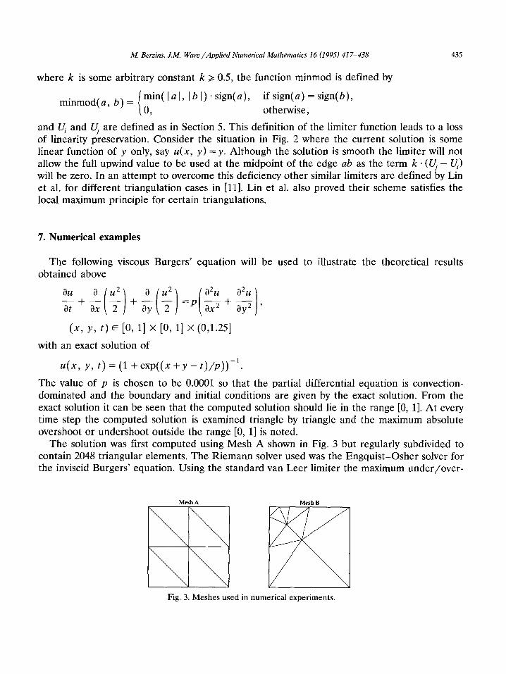
where k is some arbitrary constant k >t 0.5, the function minmod is defined by

= [ m i n ( l a l , I b I)" sign(a), if sign(a) = sign(b), minmod(a , b)

0, otherwise,

and U~ and Uj are defined as in Section 5. This definition of the limiter function leads to a loss of linearity preservation. Consider the situation in Fig. 2 where the current solution is some linear function of y only, say u(x, y) =y. Although the solution is smooth the limiter will not allow the full upwind value to be used at the midpoint of the edge ab as the term k . (Uj - U/) will be zero. In an attempt to overcome this deficiency other similar limiters are defined by Lin et al. for different triangulation cases in [11]. Lin et al. also proved their scheme satisfies the local maximum principle for certain triangulations.

7. Numerical examples

The following viscous Burgers' equation will be used to illustrate the theoretical results obtained above

- - + - - + ----Pl + ] '

(x, y, t) ~ [0, 1] x [0, 11 x (0,1.251

with an exact solution of

U(X, y, t) = (1 + exp((x + y -- t ) / p ) ) -1

The value of p is chosen to be 0.0001 so that the partial differential equation is convection- dominated and the boundary and initial conditions are given by the exact solution. From the exact solution it can be seen that the computed solution should lie in the range [0, 1]. At every time step the computed solution is examined triangle by triangle and the maximum absolute overshoot or undershoot outside the range [0, 1] is noted.

The solution was first computed using Mesh A shown in Fig. 3 but regularly subdivided to contain 2048 triangular elements. The Riemann solver used was the Engquis t -Osher solver for the inviscid Burgers' equation. Using the standard van Leer limiter the maximum under /over -

Mesh A Mesh B

Fig. 3. Meshes used in numerical experiments.

4 3 6 M. Berzins, J.M. Ware/Applied Numerical Mathematics 16 (1995) 417-438

shoot recorded was 0.0. This shows that the unmodified limiter can be used to provide oscillation-free solutions in certain circumstances.

The computation was repeated but now using Mesh B shown in Fig. 3 regularly subdivided to contain 2816 triangular elements. The maximum unde r /ove r shoo t is now 7.3369e-3 with the van Leer limiter. No overshoot was observed with the new limiter or the van Albeda limiter on ei ther mesh.

The accuracy of the schemes on this problem above is more difficult to assess due to the shock-like behaviour of the solution. In this case Mesh A is used with regular refinement. ONE is the first-order method, VL is the van Leer limiter, MVL is the modified limiter and VA is the van Albeda limiter.

The results in Table 1 show that on a shock problem for which many first-order elements are used (i.e. a flat solution or a zero limiter), all the limiters give only first-order accuracy but that the notionally second-order methods are more accurate by a factor of two. These results are consistent with those obtained by Berzins [2] on regular quadrilateral meshes.

In the light of the above results the accuracy of the method on a problem without shock-like features must be studied. Consider the solution of the linear conservation law

u,+ux+uy=O, (x,y,t)~[O, 1]X[O, 1]X(O,O.75] (46)

with exact solution

u(x, y, t) = sin(2rrx - t) sin(2rry - t ) , (47)

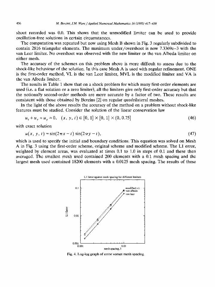
which is used to specify the initial and boundary conditions. This equation was solved on Mesh A in Fig. 3 using the first-order scheme, original scheme and modified scheme. The L1 error, weighted by e lement areas, was evaluated at times 0.1 to 1.0 in steps of 0.1 and these then averaged. The smallest mesh used contained 200 elements with a 0.1 mesh spacing and the largest mesh used contained 18200 elements with a 0.0125 mesh spacing. The results of these

t~

.5

LI Error against mesh spacing for different l imiters . . . . . . . i

0.1 modi f i ed v.l. , ~ van albeda

,,,,;,;,,c';; van leer

,~ : :"

0.01

0.1301 , , , , , ~ , , I 0.001 0.01

mesh spacing, I

Fig. 4. Log-log graph of error versus mesh spacing.

M. Berzins, J.M. Ware~Applied Numerical Mathematics 16 (1995) 417-438

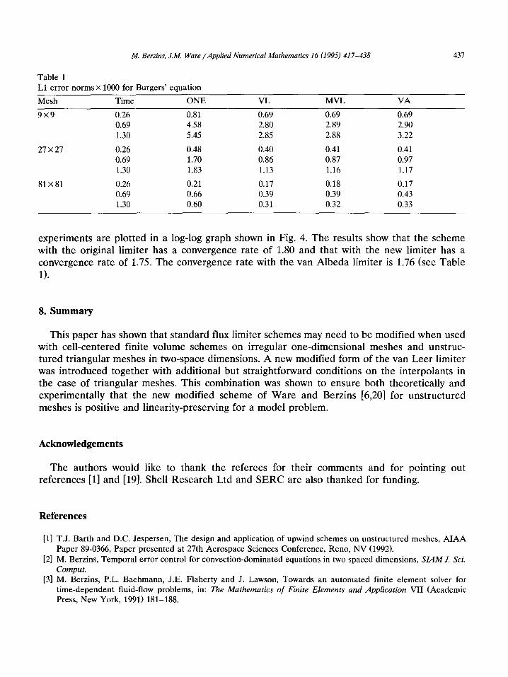
Table 1 L1 error norms x 1000 for Burgers' equation

437

Mesh Time ONE VL MVL VA

9 x 9 0.26 0.81 0.69 0.69 0.69 0.69 4.58 2.80 2.89 2.90 1.30 5.45 2.85 2.88 3.22

27 x 27 0.26 0.48 0.40 0.41 0.41 0.69 1.70 0.86 0.87 0.97 1.30 1.83 1.13 1.16 1.17

81 x 81 0.26 0.21 0.17 0.18 0.17 0.69 0.66 0.39 0.39 0.43 1.30 0.60 0.31 0.32 0.33

expe r imen t s are p lo t t ed in a log-log g raph shown in Fig. 4. T h e resul ts show that the s ch em e with the or iginal l imi ter has a conve rgence ra te of 1.80 and tha t with the new l imiter has a conve r ge nc e ra te o f 1.75. T h e conve rgence ra te with the van A l b e d a l imi ter is 1.76 (see Tab l e

1).

8. Summary

This p a p e r has shown tha t s t anda rd flux l imi ter schemes may n e e d to be mod i f i ed w h en used with ce l l - cen t e red finite vo lume schemes on i r regu la r one -d imens iona l m esh es and uns t ruc- t u r ed t r i angu la r meshes in two-space d imensions . A new modi f i ed fo rm of the van L e e r l imi ter was i n t r o d u c e d t o g e t h e r with addi t iona l bu t s t ra igh t fo rward condi t ions on the in t e rpo lan t s in the case o f t r i angula r meshes . This combina t ion was shown to en su re b o th theore t i ca l ly and expe r imen ta l ly tha t the new modi f i ed s cheme of W a r e and Berz ins [6,20] for u n s t r u c t u r e d mes he s is posi t ive and l inear i ty-preserv ing for a m o d e l p rob lem.

Acknowledgements

T h e au thor s would like to t hank the r e f e r ees for the i r c o m m e n t s and for po in t ing ou t r e f e r e nc e s [1] and [19]. Shell R e s e a r c h L td and S E R C are also t h a n k e d for funding.

References

[1] T.J. Barth and D.C. Jespersen, The design and application of upwind schemes on unstructured meshes, AIAA Paper 89-0366, Paper presented at 27th Aerospace Sciences Conference, Reno, NV (1992).

[2] M. Berzins, Temporal error control for convection-dominated equations in two spaced dimensions, SlAM J. Sci. Comput.

[3] M. Berzins, P.L. Baehmann, J.E. Flaherty and J. Lawson, Towards an automated finite element solver for time-dependent fluid-flow problems, in: The Mathematics of Finite Elements and Application VII (Academic Press, New York, 1991) 181-188.


[4] M. Berzins and R.M. Furzeland, An adaptive theta method for the solution of stiff and non-stiff differential equations, Appl. Numer. Math. 8 (1992) 1-19.

[5] M. Berzins, J.M. Ware and J. Lawson, Spatial and temporal error control in the adaptive solution of systems of conservation laws, in: Advances in Computer Methods for Partial Differential Equations, IMACS PDE VII (IMACS, New Brunswick, N J, 1992).

[6] M. Berzins and J.M. Ware, Reliable finite volume methods for time-dependent p.d.e.s, in: J.R. Whiteman, ed., Mafelap Conference (Wiley, New York, 1994).

[7] B. Cockburn, Suchung Hou and Chi-Wang Shu, The Runge-Kutta local projection discontinuous Galerkin finite element method for conservation laws IV: the multidimensional case, Math. Comp. 54 (190) (1990) 545-581.

[8] L.J. Durlofsky, B. Enquist and S. Osher, Triangle based adaptive stencils for the solution of hyperbolic conservation laws, J. Comput. Phys. 98 (1992) 64-73.

[9] Y.N. Jeng and J.L. Chen, Truncation error analysis of the finite volume method for a model steady convective equation, J. Comput. Phys. 100 (1992) 64-76.

[10] D. Kroner and M. Rokyta, Convergence of upwind finite volume schemes for scalar conservation laws in two dimensions, SIAM J. Numer. Anal 31 (1994)324-343.

[11] S.Y. Lin, T.M. Wu and Y.S. Chin, Upwind finite-volume method with a triangular mesh for conservation laws, J. Comput. Phys. 107 (1993) 324-337.

[12] X.D. Liu, A maximum principle satisfying modification of triangle based adaptive stencils for the solution of scalar hyperbolic conservation laws SIAM J. Numer. Anal. 30 (1993) 701-715.

[13] S.V. Pennington and M. Berzins, New NAG Library software for first-order P.D.E.s, ACM Trans. Math. Software 20 (1) (1994) 63-99.

[14] P.L. Roe, Characteristic based schemes for the Euler equations, Ann. Rev. Fluid Mech. 8 (1986) 337-365. [15] C.W. Shu and S. Osher, Efficient implementation of E.N.O. shock capturing schemes, J. Comput. Phys. 77

(1988) 439-471. [16] S. Spekreijse, Multigrid solution of monotone second-order discretizations of hyperbolic conservation laws,

Math. Comp. 49 (179) (1987) 135-155. [17] R. Struijs, H. Deconinck and P.L. Roe, Fluctuation splitting schemes for the 2D Euler equations, Technical

Report, von Karman Institute for Fluid Dynamics, Rhode Saint Genese, Belgium (1991). [18] B. van Leer, Progress in multi-dimensional upwind differencing, in: M. Napolitano and F. Sabetta, eds.,

Proceedings Thirteenth International Conference on Numerical Methods in Fluid Dynamics, Rome, Italy (1992). [19] V. Venkatakrishnan and T.J. Barth, Application of a direct solver to unstructured meshes for the Euler and

Navier Stokes equations. AIAA Paper 89-0364, Paper presented at 27th Aerospace Sciences Conference, Reno, NV (1992).

[20] J.M. Ware and M. Berzins, Finite volume techniques for time-dependent fluid-flow problems, in" Advances in Computer Methods for Partial Differential Equations, IMACS PDE VII (IMACS, New Brunswick, NJ, 1992).

positive cell-centered finite volume discretization …positive cell-centered finite volume...

Documents