positional accuracy handbook - mn it services

Positional AccuracyHandbookUsing the National Standard for Spatial Data Accuracyto measure and report geographic data quality

OCTOBER 1999

LAND MANAGEMENT INFORMATION CENTERMINNESOTA PLAN N I NG

The Governor’s Council on Geographic Information was created in 1991 to provide leadership inthe development, management and use of geographic information in Minnesota. With assistance fromMinnesota Planning, the council provides policy advice to all levels of government and makesrecommendations regarding investments, management practices, institutional arrangements, education,stewardship and standards.

The Council’s GIS Standards Committee was created in 1993 to help GIS users learn about and usedata standards that can help them be more productive. The committee’s Internet home page is at http://www.lmic.state.mn.us/gc/committe/stand/index.htm. This handbook was designed, researched andwritten by the committee’s Positional Accuracy Working Group: Christopher Cialek, chair, LandManagement Information Center at Minnesota Planning; Don Elwood, City of Minneapolis; Ken Johnson,Minnesota Department of Transportation; Mark Kotz, assistant chair, Minnesota Pollution Control Agency;Jay Krafthefer, Washington County; Jim Maxwell, The Lawrence Group; Glenn Radde, MinnesotaDepartment of Natural Resources; Mike Schadauer, Minnesota Department of Transportation; Ron Wencl,U.S. Geological Survey.

Minnesota Planning is charged with developing a long-range plan for the state, stimulating publicparticipation in Minnesota’s future and coordinating activities with state agencies, the Legislature andother units of government.

Upon request, the Positional Accuracy Handbook will be made available in an alternative format, such asBraille, large print or audio tape. For TTY, contact Minnesota Relay Service at 800-627-3529 and ask forMinnesota Planning.

Copies of the Positional Accuracy Handbook can be downloaded at: http://www.mnplan.state.mn.us/press/accurate.html. For additional information or printed copies of this handbook, contact the LandManagement Information Center, 651-297-2488; e-mail [email protected]. The council’s Internethome page is at http://www.lmic.state.mn.us/gc/gc.htm. Copies of the National Standard for Spatial DataAccuracy can be downloaded at: http://www.fgdc.gov/standards/status/sub1_3.html.

October 1999

658 Cedar St.St. Paul, MN 55155651-296-1211www.lmic.state.mn.us

Positional Accuracy Handbook

Using the National Standard for Spatial Data Accuracyto measure and report geographic data quality 1

CASE STUDIES

A. Large-scale data sets 9Minnesota Department of Transportation

B. Contract service work 13City of Minneapolis

C. County parcel database 15Washington County

D. Street centerline data set to whichNSSDA testing cannot be applied 23The Lawrence Group

E. Statewide watershed data set withnondiscrete boundaries 25Minnesota Department of Natural Resources

APPENDIX

National Map Accuracy Standards 28

APPLYING THE NSSDA

This example demonstrates how the Positional Accuracy Handbook helped the Minnesota Department ofTransportation make a prudent business decision.

Keeping track of the state’s tens of thousands of road signs is no simple task. When speed limits change or asign gets knocked down or simply gets old, the Minnesota Department of Transportation must install, update,repair or replace those signs. To efficiently manage this substantial resource, the department needs toaccurately identify where signs are located and ultimately, to develop a GIS system for Facilities Management.

Traditional survey methods for collecting sign locations can be time consuming and costly. This is particularlytrue when dealing with large numbers of signs spread out over a sizeable area. With thousands of signs tosurvey, mainly situated near highway traffic, Mn/DOT looked to desktop surveying to provide a safe, quick andcost-effective way to collect sign location information. Desktop surveying is the process of calculatingcoordinate information from images on a computer. The images are collected using a van equipped withmultiple cameras and geo-referenced with ground coordinates.

To evaluate this technology, Mn/DOT chose a short segment of State Trunk Highway 36 and collected x and ycoordinates for all westbound signs with desktop surveying software packages from three vendors. A Mn/DOTsurvey crew was also sent out to collect the same signs with traditional survey equipment. The task of trying tofigure out just how accurate the sign locations were for each desktop surveying package called for astandardized method; one with proven statistical merit.

Traditional methods of calculating accuracy are based on paper maps and would not work for this data. Mn/DOT turned to the draft Positional Accuracy Handbook, for a step-by-step approach and sound statisticalmethodology. The NSSDA recognizes the growing need for evaluating digital spatial data and provides acommon language for reporting accuracy. Mn/DOT used the draft handbook to complete an accuracy evaluationand to critique this new data collection method.

After the results of Mn/DOT’s Mobile Mapping Accuracy Assessment were released in May 1999, thedepartment made the decision to use desktop surveying to collect locations for all signs in the Twin Citiesmetropolitan area, about 8,000 signs along 500 miles of roadway. Confidence in the accuracy and results of thisnew data collection method will save the state valuable time and resources.

Joella M. GivensGIS Coordinator, Mn/[email protected]

Sign location comparisonsfor this section of TrunkHighway 36 in RamseyCounty indicate errors

ranging from 20centimeters to 4 meters.

POSITIONAL ACCURACY HANDBOOK 1

This handbook explains a national standard for dataquality. The National Standard for Spatial DataAccuracy describes a way to measure and reportpositional accuracy of features found within ageographic data set. Approved in 1998, the NSSDArecognizes the growing need for digital spatialdata and provides a common language for report-ing accuracy.

The Positional Accuracy Handbook offers practicalinformation on how to apply the standard to avariety of data used in geographic informationsystems. It is designed to help interpret the NSSDAmore quickly, use the standard more confidentlyand relay information about the accuracy of datasets more clearly. It is also intended to help datausers better understand the meaning of accuracystatistics reported in data sets. Case studies in thishandbook demonstrate how the NSSDA can beapplied to a wide range of data sets.

The risk of unknown accuracy

Consider this increasingly common spatial dataprocessing dilemma. An important project requiresthat the locations of certain public facilities beplotted onto road maps so service providers mayquickly and easily drive to each point. Global Posi-tioning System receivers use state-of-the-artsatellite technology to pinpoint the required loca-

tions. To provide context, these facility locationsare then laid over a digital base map containingroads, lakes and rivers. A plot of the results revealsa disturbing problem: some facilities appear to belocated in the middle of lakes (see figure 1).

Which data set is correct: the base map or thefacility locations? No information about positionalaccuracy was provided for either data set, butintuition would lead us to believe that GPS pointsare much more accurate than information collectedfrom a 1:100,000-scale paper map. Right?

In this case, wrong. The GPS receivers used for thisstudy were only accurate to within 300 feet. Thebase map was assumed to be accurate to within167 feet because it complied with the 1947 NationalMap Accuracy Standards. In reality, the base mapmay be almost twice as accurate as the informa-tion gathered from a state-of-the-art network ofsatellites. But, how would a project manager everbe able to know this simply by looking at a displayon a computer screen?

Five components of data quality

This example illustrates an important principle ofgeographic information systems. The value of anygeographic data set depends less on its cost, andmore on its fitness for a particular purpose. A criticalmeasure of that fitness is data quality. When usedin GIS analysis, a data set’s quality significantlyaffects confidence in the results. Unknown dataquality leads to tentative decisions, increasedliability and loss of productivity. Decisions basedon data of known quality are made with greaterconfidence and are more easily explained anddefended. Federal standards that assist in docu-menting and transferring data sets recognize fiveimportant components of data quality:

Positional accuracy. How closely thecoordinate descriptions of features compare totheir actual location.

Attribute accuracy. How thoroughly andcorrectly the features in the data set are described.

Figure 1. Variations indata accuracy are

apparent when the twodata sets are merged as

shown here. The blackflag marks the reported

location of a buildingwith a 5th Street address

collected from a GPSreceiver. Lake and road

data come from U.S.Bureau of the Census.

Positional Accuracy HandbookUsing the National Standard for Spatial Data Accuracy to measure and report geographic data quality

2 POSITIONAL ACCURACY HANDBOOK

Logical consistency. The extent to whichgeometric problems and drafting inconsistenciesexist within the data set.

Completeness. The decisions that determinewhat is contained in the data set.

Lineage. What sources are used to constructthe data set and what steps are taken to processthe data.

Considered together, these characteristics indicatethe overall quality of a geographic database. Theinformation contained in this handbook focuses onthe first characteristic, positional accuracy.

Why a new standard is needed

How the positional accuracy of map features isbest estimated has been debated since the earlydays of cartography. The question remains a sig-nificant concern today with the proliferating use ofcomputers, geographic information systems anddigital spatial data. Until recently, existing accu-racy standards such as the National Map AccuracyStandards (described in the appendix) focused ontesting paper maps, not digital data.

Today, use of digital GIS is replacing traditionalpaper maps in more and more applications. Digitalgeographic data sets are being generated by fed-eral, state and local government agencies, utilities,businesses and even private citizens. Determiningthe positional accuracy of digital data is difficultusing existing standards.

A variety of factors affect the positional accuracyof digital spatial data. Error can be introduced by:digitizing methods, source material, generalization,symbol interpretation, the specifications of aerialphotography, aerotriangulation technique, groundcontrol reliability, photogrammetric characteristics,scribing precision, resolution, processing algo-rithms and printing limitations. Individual errorsderived from any one of these sources is oftensmall; but collectively, they can significantly affectdata accuracy, impacting how the data can beappropriately used.

The NSSDA helps to overcome this obstacle byproviding a method for estimating positional accu-racy of geographic data, in both digital and printedform.

The National Standard for Spatial Data Accuracy isone in a suite of standards dealing with the accu-racy of geographic data sets and is one of the mostrecent standards to be issued by the Federal Geo-graphic Data Committee. Minnesota was

represented in the latter stages of the standard’sdevelopment through the Governor’s Council onGeographic Information and the state’s Depart-ment of Transportation.

The role of the NSSDA in datadocumentation

The descriptive information that accompanies adata set is often referred to as metadata. Practi-cally speaking, a well-documented data set is onethat has a metadata record, including a standardreport of positional accuracy based on NSSDAmethods. Well documented and tested data setsprovide an organization with a clear understandingof its investment in information resources. Trust-worthy documentation also provides data userswith an important tool when evaluating data fromother sources. More information about metadatacan be found in this handbook on page 7.

How the NSSDA works

There are seven steps in applying the NSSDA:

1. Determine if the test involves horizontalaccuracy, vertical accuracy or both.

2. Select a set of test points from the data setbeing evaluated.

3. Select an independent data set of higheraccuracy that corresponds to the data set beingtested.

4. Collect measurements from identical pointsfrom each of those two sources.

5. Calculate a positional accuracy statistic usingeither the horizontal or vertical accuracy statisticworksheet.

6. Prepare an accuracy statement in a standardizedreport form.

7. Include that report in a comprehensive descrip-tion of the data set called metadata.

FEATURES OF THE NSSDAIdentifies a well-defined statistic used to

describe accuracy test results

Describes a method to test spatial data forpositional accuracy

Provides a common language to reportaccuracy that makes it easier to evaluate the“fitness for use” of a database


Steps in detail

1. Determining which test to use. The firststep in applying the NSSDA is to identify the spa-tial characteristics of the data set being tested. Ifplanimetric accuracy — the x,y accuracy — of thedata set is being evaluated, use the horizontalaccuracy statistic worksheet (see figure 4). If eleva-tion accuracy — z accuracy — is being evaluated,use the vertical accuracy worksheet (see figure 5).

2. Selecting test points. A data set’s accuracyis tested by comparing the coordinates of severalpoints within the data set to the coordinates of thesame points from an independent data set ofgreater accuracy. Points used for this comparisonmust be well-defined. They must be easy to findand measure in both the data set being tested andin the independent data set.

For data derived from maps at a scale of 1:5,000 orsmaller, points found at right-angle intersections oflinear features work well. These could be right-angleintersections of roads, railroads, canals, ditches,trails, fences and pipelines. For data derived frommaps at scales larger than 1:5,000 — plats orproperty maps, for example — features like utilityaccess covers, intersections of sidewalks, curbs orgutters make suitable test points. For survey datasets, survey monuments or other well-markedsurvey points provide excellent test points.

Twenty or more test points are required to conducta statistically significant accuracy evaluation regard-less of the size of the data set or area of coverage.Twenty points make a computation at the 95 per-cent confidence level reasonable. The 95 percentconfidence level means that when 20 points aretested, it is acceptable that one point may exceedthe computed accuracy.

If fewer than 20 test points are available, anotherFederal Geographic Data Committee standard, theSpatial Data Transfer Standard, describes threealternatives for determining positional accuracy:1) deductive estimate, 2) internal evidence and3) comparison to source. For more information onthis federal standard, point your browser tomcmcweb.er.usgs.gov/sdts/

3. Selecting an independent data set. Theindependent data set must be acquired separatelyfrom the data set being tested. It should be of thehighest accuracy available.

In general, the independent data set should bethree times more accurate than the expected accu-racy of the test data set. Unfortunately, this is notalways possible or practical. If an independentdata set that meets this criterion cannot be found,a data set of the highest accuracy feasible shouldbe used. The accuracy of the independent data setshould always be reported in the metadata.

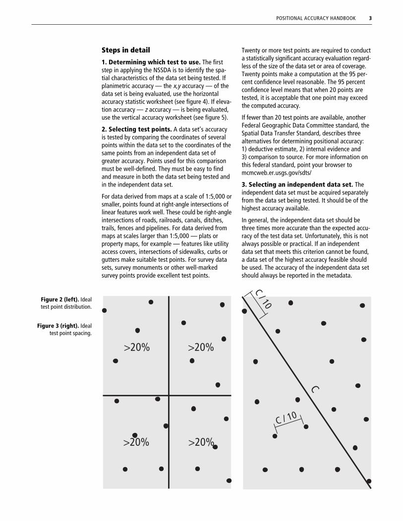
Figure 2 (left). Idealtest point distribution.

Figure 3 (right). Idealtest point spacing.

>20% >20%

>20% >20%

C / 10

C

C / 10


The areal extent of the independent data setshould approximate that of the original data set.When the tested data set covers a rectangular areaand is believed to be uniformly accurate, an idealdistribution of test points allows for at least 20percent to be located in each quadrant (see figure2). Test points should be spaced at intervals of atleast 10 percent of the diagonal distance acrossthe rectangular data set; the test points shown infigure 3 comply with both these conditions.

It is not always possible to find test points that areevenly distributed. When an independent data setcovers only a portion of a tested data set, it canstill be used to test the accuracy of the overlappingarea. The goal in selecting an independent data setis to try to achieve a balance between one that ismore accurate than the data set being tested andone which covers the same region.

Independent data sets can come from a variety ofsources. It is most convenient to use a data set thatalready exists, however, an entirely new data setmay have to be created to serve as control for thedata set being tested. In all cases, the independentand test data sets must have common points. Alwaysreport the specific characteristics of the indepen-dent data set, including its origin, in the metadata.

4. Recording measurement values. The nextstep is to collect test point coordinate values fromboth the test data set and the independent data set.When collecting these numbers, it is important torecord them in an appropriate and similar numericformat. For example, if testing a digital databasewith an expected accuracy of about 10 meters, itwould be overkill to record the coordinate values

to the sixth decimal place; the nearest meterwould be adequate. Use similar common sensewhen recording the computed accuracy statistic.

5. Calculating the accuracy statistic. Oncethe coordinate values for each test point from thetest data set and the independent data set havebeen determined, the positional accuracy statisticcan be computed using the appropriate accuracystatistic worksheet. Illustrations of filled outworksheets can be found in the handbook’s casestudies.

The NSSDA statistic is calculated by first filling outthe information requested in the appropriate tableand then computing three values:

the sum of the set of squared differencesbetween the test data set coordinate values andthe independent data set coordinate values,

the average of the sum by dividing the sum bythe number of test points being evaluated, and

the root mean square error statistic, whichis simply the square root of the average.

The NSSDA statistic is determined by multiplyingthe RMSE by a value that represents the standarderror of the mean at the 95 percent confidencelevel: 1.7308 when calculating horizontal accuracy,and 1.9600 when calculating vertical accuracy.

Accuracy statistic worksheets may be downloadedoff the Internet from LMIC’s positional accuracy webpage (www.mnplan.state.mn.us/press/accurate.html) and clicking on Download accuracystatistic worksheets.

THE FEDERAL GEOGRAPHIC DATA COMMITTEE

The FGDC is a consortium of 16 federal agencies created in 1989 to better coordinate geographic datadevelopment across the nation. Additional stakeholders include: 28 states, the National Association of Countiesand the National League of Cities, as well as other groups representing state and local government and theacademic community. The Minnesota Governor’s Council on Geographic Information represents the state on theFGDC. The committee has created a model for coordinating spatial data development and use. The NationalSpatial Data Infrastructure promotes efficient use of geographic information and GIS at all levels of governmentthrough three initiatives:

Standards. Developing common ways of organizing, describing and processing geographic data to ensurehigh quality and efficient sharing.

Clearinghouse. Providing Internet access to information about data resources available for sharing.

Framework data. Defining the basic data layers needed for nearly all GIS analysis; better design offramework data layers promises easier data sharing.

For more information about the FGDC, visits its web site at www.fgdc.gov. The committee has set ambitiousgoals to identify areas where standards are needed and to develop those standards together with its partners.Details about committee-sponsored standards, both under development and completed, can be found on theGovernor’s Council web site at: www.lmic.state.mn.us/gc/standards.htm and at www.fgdc.gov/standards

AKOEBRICK

Cross-Out

AKOEBRICK

Replacement Text

http://www.mngeo.state.mn.us/resource.html?Id=1852

https://www.mngeo.state.mn.us/committee/standards/positional_accuracy/index.html


A B C D E F G H I J KPoint

numberPoint

descriptionx (inde-

pendent) x (test) diff in x (diff in x) 2 y (inde-pendent) y (test) diff in y (diff in y) 2 (diff in x) 2 +

(diff in y) 2

sum

average

RMSEr

NSSDA

Column Title Content

A Point number Designator of test point

B Point description Description of test point

C x (independent) x coordinate of point from independent data set

D x (test) x coordinate of point from test data set

E diff in x x (independent) - x (test)

F ( diff in x ) 2 Squared difference in x = ( x (independent) - x (test) ) 2

G y (independent) y coordinate of point from independent data set

H y (test) y coordinate of point from test data set

I diff in y y (independent) - y (test)

J ( diff in y ) 2 Squared difference in y = ( y (independent) - y (test) ) 2

K ( diff in x ) 2 + ( diff in y ) 2 Squared difference in x plus squared difference in y = (error radius)2

sum ∑ [(diff in x ) 2 + (diff in y ) 2 ]average sum / number of pointsRMSEr Root Mean Square Error (radial) = average1/2

NSSDA National Standard for Spatial Data Accuracy statistic = 1.7308 * RMSEr

Figure 4. Horizontalaccuracy statistic

worksheet.


Column Title Contents

A Point number Designator of test point

B Point description Description of test point

C z (independent) z coordinate of point from independent data set

D z (test) z coordinate of point from test data set

E diff in z z (independent) - z (test)

F ( diff in z ) 2 Squared difference in z = ( z (independent) - z (test) ) 2

sum ∑ (diff in z ) 2

average sum / number of pointsRMSE Root Mean Square Error (vertical) = average1/2

NSSDA National Standard for Spatial Data Accuracy statistic = 1.9600 * RMSE

A B C D E FPoint

numberPoint

descriptionz (inde-

pendent) z (test) diff in z (diff in z) 2

sum

average

RMSEz

NSSDA

Figure 5. Verticalaccuracy statistic

worksheet.


6. Preparing an accuracy statement. Oncethe positional accuracy of a test data set has beendetermined, it is important to report that value in aconsistent and meaningful way. To do this one oftwo reporting statements can be used:

Tested _____ (meters, feet) (horizontal, vertical)accuracy at 95% confidence level

Compiled to meet _____ (meters, feet)(horizontal, vertical) accuracy at 95% confidencelevel

A data set’s accuracy is reported with the testedstatement when its accuracy was determined bycomparison with an independent data set ofgreater accuracy as described in steps 2 through 5.For example, if after comparing horizontal testdata points against those of an independent dataset, the NSSDA statistic is calculated to be 34.8feet, the proper form for the positional accuracyreport is:

Positional Accuracy: Tested 34.8 feet horizontalaccuracy at 95% confidence level

This means that a user of this data set can beconfident that the horizontal position of a well-defined feature will be within 34.8 feet of its truelocation, as best as its true location has been de-termined, 95 percent of the time.

When the method of compiling data has beenthoroughly tested and that method produces aconsistent accuracy statistic, the compiled to meetreporting statement can be used. Expanding on thesame example, suppose the method of data collec-tion consistently yields a positional accuracystatistic that was no worse — that is, no lessaccurate — than 34.8 feet for eight data setstested. It would be appropriate to skip the testingprocess for data set nine, and assume that itsaccuracy is consistent with previously tested data.Report this condition using the following format:

Positional Accuracy: Compiled to meet 34.8 feethorizontal accuracy at 95% confidence level

To appropriately use the compiled to meet report-ing statement, it is imperative that the data setcompilation method consists of standard, well-documented, repeatable procedures. It is alsoimportant that several data sets be produced andtested. Finally, the NSSDA statistics computed ineach test must be consistent. Once all these criteriaare met, future data sets compiled by the samemethod do not have to be tested. The largest — orworst case — NSSDA statistic from all tests isalways reported in the compiled to meet statement.

7. Including the accuracy report in metadata.The final step is to report the positional accuracy ina complete description of the data set. Often de-scribed as data about data, metadata lists thecontent, quality, condition, history and other char-acteristics of a data set.

The Minnesota Governor’s Council on GeographicInformation has established a formal method fordocumenting geographic data sets called theMinnesota Geographic Metadata Guide-lines. The guidelines are a compatible subset ofthe federal Content Standards for Digital GeospatialMetadata intended to simplify the process of creat-ing metadata. A software program called DataLogreases the task of collecting metadata that adheresto the Minnesota guidelines.

To report the positional accuracy of a data set,complete the appropriate field in section 2 of themetadata guidelines (see figures 6 and 7). Thehorizontal and vertical positional accuracy reportsare free text fields and can be filled out the sameway. Write the entire accuracy report statementfollowed by an explanation of how the accuracyvalue was determined and any useful characteris-tics of the independent data set.

Potential users of the data set might find this typeof additional information useful:

Specifically stating that the National Standard forSpatial Data Accuracy was used to test the data set.

POSITIONAL ACCURACY DESCRIPTIONS IN THE FEDERAL METADATA STANDARD

Section 2.4 of the full federal Content Standards for Digital Geospatial Metadata contains a number ofpositional accuracy related fields:

The NSSDA statistic should be placed in field 2.4.1.2.1 for horizontal accuracy and in field 2.4.2.2.1 for verticalaccuracy. The text string “National Standard for Spatial Data Accuracy” should be entered in field 2.4.1.2.2 forhorizontal accuracy and in field 2.4.2.2.2 for vertical accuracy.

Finally, an explanation of how the accuracy value was determined can be included in the horizontal positionalaccuracy report fields: 2.4.1.1 for horizontal and 2.4.2.1 for vertical.


Describing what is known about the variabilityof accuracy across the data set.

Pointing users to other sections of the metadatafor more information.

Testing the NSSDA

Case studies in this handbook offer practical ex-amples of how the NSSDA was applied to aselection of widely varied data sets. Each examplestrives to employ the procedures described here,and each offers a unique approach in establishingaccuracy measurements due to the distinctiveconditions of the test data set, the independentsource and other local characteristics. Positionalaccuracy in these examples ranges from specific togeneral, from 0.2 meter to 4,800 meters, providingNSSDA users with ideas of how to adapt the stan-dard to their own data sets.

To find out more about standards, metadata guide-lines and DataLogr, go to www.lmic.state.mn.us andlook under Spatial Data Standards, or contact LMICby e-mail at [email protected] orcall Christopher Cialek at 651-297-2488.

ReferencesAmerican National Standards Institute, 1998. Information

Technology — Spatial Data Transfer Standard (SDTS)ANSI-NCITS 320. New York, mcmcweb.er.usgs.gov/sdts/

American Society for Photogrammetry and RemoteSensing, Specifications and Standards Committee,1990. “ASPRS Accuracy Standards for Large-ScaleMaps,” Photogrammetric Engineering & RemoteSensing. Washington, D.C., v56, no7, pp1068-1070.

Federal Geographic Data Committee, 1998. GeospatialPositioning Accuracy Standards; Part 3: NationalStandard for Spatial Data Accuracy, FGDC-STD-007.3.Federal Geographic Data Committee. Washington,D.C. www.fgdc.gov/standards/status/sub1_3.html

Federal Geographic Data Committee, 1998. ContentStandards for Digital Geospatial Metadata (version2.0), FGDC-STD-001. Federal Geographic Data Com-mittee. Washington, D.C. www.fgdc.gov/standards/status/csdgmovr.html

Greenwalt, C.R. and Shultz, M.E. Principles of errortheory and cartographic applications; Technical ReportNo. 96, 1962. U.S. Air Force Aeronautical Chart andInformation Center. St. Louis, Missouri.

Minnesota Governor’s Council on Geographic Informa-tion. Minnesota Geographic Metadata Guidelines(version 1.2), 1998. St. Paul, Minnesota.www.lmic.state.mn.us/gc/stds/metadata.htm

U.S. Bureau of the Budget. U.S. National Map AccuracyStandards,1947. Washington, D.C.

Figure 6. Formal NSSDAaccuracy statements

reported in section 2 ofthe Minnesota

Geographic MetadataGuidelines.

Horizontalpositionalaccuracy

Tested 0.181 meters horizontal accuracy at 95% confidence level.

Verticalpositionalaccuracy

Tested 0.134 meters vertical accuracy at 95% confidence level.

Figure 7. An example ofa detailed positional

accuracy statement asreported in metadata.


Digitized features outside areas of high vertical relief: tested 23 feet horizontal accuracy atthe 95% confidence level using the NSSDA.

Digitized features within areas of high vertical relief (such as major river valleys): tested 120feet horizontal accuracy by other testing procedures.

For a complete report of the testing procedures used, contact Washington County Surveyor’sOffice as noted in Section 6, Distribution Information.

All other features are generated by coordinate geometry and are based on a framework ofaccurately located PLSS corner positions used with public information of record. Computedpositions of parcel boundaries are not based on individual field surveys. Although tests ofrandomly selected points for comparison may show high accuracy between field and parcelmap content, variations between boundary monumentation and legal descriptions of recordcan and do exist. Caution is necessary when using land boundary data shown. Contact theWashington County Surveyor’s Office for more information.


Not applicable


Case Study A

Minnesota Department of TransportationApplying the NSSDA to large-scale data sets

The project

This project evaluates the accuracy of topographicand digital terrain model data sets created usingphotogrammetric techniques. The Minnesota De-partment of Transportation’s photogrammetric unitproduces these data sets, which are used withinthe agency to plan and design roadways and road-way improvements.

The horizontal accuracy of the topographic dataset was tested. Although the elevation contours ofthe topographic data set do record vertical data, adifferent data set, a Digital Terrain Model, wasused to test vertical accuracy, as DTMs tend to bemore accurate. DTMs are used to compute complexsolutions dealing with design issues such as mate-rial quantities and hydraulics. To rely on thesesolutions, understanding the accuracy of the DTMis crucial.

The tested data set

The two data sets consist of digital elevation con-tours and a digital terrain model created from 457meter altitude, 1:3000 scale aerial photography.They cover a corridor on Interstate Highway 94from Earl Street to the junction of interstates 494and 694, east of St. Paul. The mapping widthvaries from 250 meters to 862 meters and aver-ages 475 meters. The horizontal accuracy, reflectedin the digital topographic map, and the verticalaccuracy, reflected in the digital terrain model,both were tested.

The independent data set

Mn/DOT’s photogrammetric unit has historicallyassessed digital terrain models for vertical accu-racy using National Map Accuracy Standards. Thetraditional method of evaluating vertical accuracywas to perform a test on every fourth model, orstereo pair, throughout the corridor. In each testedmodel, the x, y and z field coordinates of 20 ran-dom points were collected using Geotracer DualFrequency GPS receivers with an expected accuracy

of 10-15 mm (rms). The z coordinate from the fieldwas compared to the z coordinate from the corre-sponding x and y coordinates in the digital terrainmodel to determine if they met the standard: 90percent of the points fall within one half contour.

This project has 13 test models. With about 20points in every test model there are 296 controlpoints available for the entire corridor. Eventhough this is far more than the minimum sug-gested by the National Standard for Spatial DataAccuracy, the points were already measured so allwere used.

The selection of control points for vertical accuracytesting was very simple. The survey field crewselected about 20 random points in every fourthmodel. These did not have to be well-definedpoints in the horizontal dimension because theywere only intended to evaluate the vertical accu-racy of the digital terrain model. As long as thecontrol points were within the extent of the digitalterrain model, they served to help evaluate thedigital terrain model’s vertical accuracy.

The digital topographic map made from the sameaerial photography was not originally assessed forhorizontal accuracy; however, it complied withNational Map Accuracy Standards, which varybased on the scale of the map. It was assumedthat, if horizontal problems existed, they would beuncovered and addressed when field crews con-ducted additional surveys to supplement themapping.

This meant that there were no preconceived meth-ods for assessing the horizontal accuracy. Themethod chosen for this example was to collect thecoordinates of 40 well-defined points throughoutthe corridor. Geotracer Dual Frequency GPS receiv-ers were used. Data was collected using a faststatic method with an expected accuracy of 10-15mm (rms).

In selecting the 40 control points used to assessthe vertical accuracy, the project team chose pointsthat were well defined both on the topographic

PROJECT TEAM

Ken JohnsonGeodetic servicesengineer

Mike LallaPhotogrammetry mappingsupervisor

Mike SchadauerLand information systemsengineer


map and in the field, and were fairly evenly distrib-uted throughout the corridor. Examples of theseinclude manholes, catch basins and right-angleintersections of objects such as sidewalks. Fortypoints were chosen rather than the minimum of 20because they were fairly easy to collect and becauseof the long narrow shape of the corridor. Havingthe extra points opened the possibility of compar-ing a test of the 20 easternmost control pointswith a test of the 20 westernmost control points.

The worksheet

The completed worksheets for the vertical andhorizontal accuracy testing are shown in tables A.1and A.2, respectively. The columns listed as inde-pendent are the GPS collected points. The columnslisted as test are the photogrammetrically derivedpoints taken off the DTM for the vertical test andthe topographic map for the horizontal test.

Pointnumber

z (test)Photo elev

z (independent)Field elev

diff in zPhoto field (diff in z) 2

100 293.755 293.79 -0.035 0.001202

101 293.671 293.71 -0.039 0.001515

102 293.87 293.9 -0.03 0.000913

103 293.815 293.85 -0.035 0.001241

104 294.609 294.62 -0.011 0.000113

105 295.238 295.3 -0.062 0.003834

106 295.54 295.56 -0.02 0.000394

107 295.28 295.3 -0.02 0.000385

108 294.933 295 -0.067 0.004465

109 294.431 294.46 -0.029 0.000847

110 293.994 294.02 -0.026 0.000664

111 293.736 293.77 -0.034 0.001131

112 293.537 293.58 -0.043 0.001886

113 293.478 293.55 -0.072 0.005164

114 293.671 293.7 -0.029 0.000858

115 293.949 293.97 -0.021 0.000425

116 294.427 294.49 -0.063 0.00402

117 294.837 294.88 -0.043 0.001881

118 295.19 295.28 -0.09 0.008062

119 295.318 295.31 0.008 0.000057

581 259.435 259.42 0.015 0.000213

582 258.766 258.74 0.026 0.000682

583 258.603 258.61 -0.007 0.000046

584 258.71 258.72 -0.01 0.000105

585 259.407 259.39 0.017 0.000275

586 259.285 259.28 0.005 0.000022

587 259.41 259.43 -0.02 0.000405

588 260.017 260.02 -0.003 0.000008

589 260.596 260.67 -0.074 0.005473

590 261.801 261.84 -0.039 0.001513

592 263.428 263.42 0.008 0.00007

593 256.949 256.93 0.019 0.000352

594 256.853 256.82 0.033 0.001105

595 256.766 256.72 0.046 0.002095

596 256.411 256.39 0.021 0.000441

597 256.12 256.14 -0.02 0.000414

598 258.249 258.3 -0.051 0.002645

599 258.395 258.46 -0.065 0.004181

600 258.414 258.46 -0.046 0.002159

sum 1.375

average 0.005

RMSEz 0.068

NSSDA 0.134

Table A.1. Verticalaccuracy statistic

worksheet.


Pointnumber

Pointdescription

x (inde-pendent)

x (test) diff in x(diff

in x) 2y (inde-

pendent)y (test) diff in y

(diffin y) 2

(diff in x) 2 +(diff in y) 2

1 TP1A 178247.28 178247.37 -0.089 0.007921 48326.075 48326.135 -0.06 0.0036 0.011521

2 TP2 178249.23 178249.17 0.055 0.003025 48287.228 48287.171 0.057 0.003249 0.006274

3 TP3A 178456.79 178456.73 0.06 0.0036 48337.408 48337.283 0.125 0.015625 0.019225

4 TP4 178715.82 178715.88 -0.054 0.002916 48542.511 48542.543 -0.032 0.001024 0.00394

5 TP5 179047.54 179047.65 -0.104 0.010816 48657.388 48657.44 -0.052 0.002704 0.01352

6 TP6 179227.78 179227.8 -0.016 0.000256 48336.177 48336.147 0.03 0.0009 0.001156

7 TP7 179238.56 179238.69 -0.132 0.017424 48671.457 48671.48 -0.023 0.000529 0.017953

9 TP9 180257.36 180257.39 -0.033 0.001089 48337.972 48337.97 0.002 4E-06 0.001093

10 SWK 180426.36 180426.36 0.005 2.5E-05 48445.001 48444.917 0.084 0.007056 0.007081

11 DI 180568.35 180568.48 -0.128 0.016384 48523.693 48523.696 -0.003 9E-06 0.016393

12 TP12A 180680.73 180680.78 -0.053 0.002809 48275.075 48274.978 0.097 0.009409 0.012218

13 SW 180676.31 180676.38 -0.076 0.005776 48413.085 48413.154 -0.069 0.004761 0.010537

14 TP14 180654.46 180654.47 -0.01 0.0001 47955.055 47954.992 0.063 0.003969 0.004069

15 MH 180843.48 180843.56 -0.083 0.006889 48505.391 48505.548 -0.157 0.024649 0.031538

17 TP17 181338.97 181339.11 -0.141 0.019881 48313.103 48313.244 -0.141 0.019881 0.039762

18 TP18 181283.2 181283.25 -0.051 0.002601 48174.063 48174.057 0.006 3.6E-05 0.002637

19 TP19 181075.07 181075.09 -0.018 0.000324 48171.737 48171.637 0.1 0.01 0.010324

20 TP20A 181495.79 181495.85 -0.057 0.003249 48043.414 48043.497 -0.083 0.006889 0.010138

21 TP21 181679.58 181679.59 -0.009 8.1E-05 48242.779 48242.744 0.035 0.001225 0.001306

22 TP22 181673.86 181673.82 0.044 0.001936 48579.533 48579.693 -0.16 0.0256 0.027536

24 TP24 181937.26 181937.3 -0.045 0.002025 48136.264 48136.256 0.008 6.4E-05 0.002089

26 TP26 182085.95 182085.96 -0.004 1.6E-05 48127.717 48127.778 -0.061 0.003721 0.003737

27 TP27 182243.61 182243.57 0.041 0.001681 48032.915 48032.879 0.036 0.001296 0.002977

28 TP28 182289.49 182289.56 -0.065 0.004225 48729.272 48729.211 0.061 0.003721 0.007946

29 TP29 182259.51 182259.63 -0.122 0.014884 48630.614 48630.707 -0.093 0.008649 0.023533

30 TP30 182277.52 182277.57 -0.053 0.002809 48410.278 48410.398 -0.12 0.0144 0.017209

32 TP32 182590.79 182590.88 -0.095 0.009025 48437.482 48437.633 -0.151 0.022801 0.031826

33 TP33 182494.13 182494.22 -0.099 0.009801 48422.78 48422.862 -0.082 0.006724 0.016525

34 TP34 182410.21 182410.24 -0.027 0.000729 48672.544 48672.564 -0.02 0.0004 0.001129

35 TP35 182740.18 182740.15 0.027 0.000729 48307.436 48307.447 -0.011 0.000121 0.00085

36 TP36 182771.78 182771.77 0.015 0.000225 47967.3 47967.292 0.008 6.4E-05 0.000289

37 TP37 183067.28 183067.27 0.014 0.000196 48044.513 48044.539 -0.026 0.000676 0.000872

38 TP38 183242.23 183242.18 0.048 0.002304 47952.797 47952.798 -0.001 1E-06 0.002305

39 TP39 183458.2 183458.24 -0.035 0.001225 47885.194 47885.162 0.032 0.001024 0.002249

40 TP40 183778.2 183778.26 -0.059 0.003481 48230.799 48230.753 0.046 0.002116 0.005597

41 TP41 183886.38 183886.4 -0.019 0.000361 47924.349 47924.264 0.085 0.007225 0.007586

42 TP42 184394.5 184394.54 -0.031 0.000961 48083.648 48083.657 -0.009 8.1E-05 0.001042

43 TP43A 184644.38 184644.44 -0.059 0.003481 48068.904 48068.751 0.153 0.023409 0.02689

44 TP44 184804.19 184804.35 -0.16 0.0256 48192.963 48192.891 0.072 0.005184 0.030784

45 TP45 185120.62 185120.67 -0.054 0.002916 48201.523 48201.505 0.018 0.000324 0.00324

sum 0.436896

average 0.0109224

RMSE 0.10451029

NSSDA 0.1808864

Table A.2. Horizontalaccuracy statistic

worksheet.

The positional accuracy statistic

The vertical root mean square error is shown as alinear error. In table A.1, the vertical RMSE is0.068 m.

The horizontal RMSE deals with two dimensionsgiving x and y coordinates. Using the equation of acircle:

x 2 + y 2 = r 2

and modifying it slightly into

( xindependent - xtest)2 +( yindependent - ytest) 2 = rerror 2

the error radius is found for each coordinate. Thehorizontal RMSE is calculated by adding up theradius errors, averaging them and taking thesquare root. This gives a circular error defined bythe radius. The horizontal RMSE in table A.2 is acircle defined by a radius of 0.105 m.


The NSSDA requires a 95 percent confidence level.To attain this, the vertical RMSE is multiplied by1.96 and the horizontal RMSE is multiplied by1.7308, resulting in horizontal and vertical accura-cies of 0.181 and 0.134 meters respectively.

The accuracy statement and metadata

Figure A.1 contains formal NSSDA reports for boththe horizontal and vertical positional accuracymeasured for this project.

Observations and comments

A couple of concerns were raised in applying theNSSDA to this data set. First, the field test shots

need to be points that have been placed on themap. For this project, the field crew substituted afew points that had not been originally placed onthe topographic maps, so these were not consid-ered. The second concern dealt with map symbolplacement, origin and scale. For example, with amap symbol such as a catch basin, the origin is thelower left corner. The field crew may have col-lected the control point using the center of thecatch basin, and even if they used the correctcorner, the scaled size may be different. This typeof systematic error could have a major impact onthe accuracy statement of this project.


Using the National Standard for Spatial Data Accuracy, the data set tested 0.181 metershorizontal accuracy at 95% confidence level.


Using the National Standard for Spatial Data Accuracy, the data set tested 0.134 metersvertical accuracy at 95% confidence level.

Figure A.1. Positionalaccuracy statements as

reported in metadata.


Case Study B

City of MinneapolisApplying the NSSDA to contract service work

PROJECT TEAM

Don ElwoodEngineer, engineeringdesign

Tara MuganeEngineer, engineeringdesign

Lisa ZickEngineering graphicsanalyst, engineeringdesign

The project

The city of Minneapolis uses its planimetric data-base for a variety of engineering and planningpurposes. In this project, it provided a photo controlto produce a digital orthophoto database for the city.

Presently, about two-thirds of Minneapolis is cov-ered with high-resolution color digitalorthophotographs. The primary use for this data-base is to identify changes over time and transferthem to the planimetric database. Updatedplanimetry is digitized from digital orthophotosinto the planimetric database. A precise matchbetween the orthophoto products and the plani-metric database is critical as design crews use theplanimetric database and orthophotos for streetdesign plans. For this reason, it was a worthwhileinvestment to develop a positional accuracy esti-mate for digital orthophotos using the NSSDA.

The tested data set

Orthophotographs are being generated by contractfrom aerial photography of a flight height of ap-

proximately 3,000 feet. The photos are beingscanned at a resolution of 25-30 microns creatingan 80-megabyte file per quarter section area.Photo distortions are removed through a procedurethat applies elevation and horizontal control to thescanned photos. This process results in a colororthophoto with a ground pixel resolution of one-half foot. Many of the images have a qualitysufficient to identify cracks in pavement surface.

As with traditional aerial photography projects,photo control on painted targets placed at regularintervals around the city was required. In addition,the vendor was required to use the city’s planimet-ric basemap for control and to supply the city withcoordinate values for those targets.


Survey monument locations from the planimetricdatabase were used as the source of independentdata. City survey crews painted targets on theexisting monuments within the flight area, at-tempting to select targets on the corner of eachquarter section. The city compared the coordinateresults from the orthophoto vendor with the con-trol data and a plot was made to show areas of“control quality.” Figure B.1 illustrates the use ofpoints to display the range between the indepen-dent data and vendors values while the arrowsshow the direction the vendor’s coordinates are incomparison to the independent data. Errors areinvestigated and additional control is providedwhere needed before the vendor starts orthophotoproduction.

The worksheet

Table B.1 contains a partial list of coordinate val-ues for the independent (monument) coordinates,test (vendor) coordinates, the differences betweeneach of those values and the squared difference for126 monuments. From these values a sum, aver-age, root mean square error and National Standardfor Spatial Data Accuracy statistic are calculated.

Figure B.1. Portion of aMinneapolis control

quality map identifyingthe magnitude and

direction of differencesbetween city monuments

and correspondingvendor-supplied data.


Pointnumber

x (inde-pendent)

x (test) diff in x(diff in

x)2y (inde-

pendent)y (test)

diff iny

(diff iny)2

(diff in x) 2

+ (diff in y) 2

3234 542850.895 542850.872 0.023 0.000529 152223.812 152223.840 -0.028 0.000784 0.001313

3062 522260.248 522260.211 0.037 0.001369 138937.691 138937.700 -0.009 8.1E-05 0.00145

118 541542.816 541542.781 0.035 0.001225 141704.350 141704.309 0.041 0.001681 0.002906

230A 540484.021 540484.057 -0.036 0.001296 148882.295 148882.347 -0.052 0.002704 0.004

441 535191.599 535191.550 0.049 0.002401 161295.030 161295.075 -0.045 0.002025 0.004426

811 539143.822 539143.898 -0.076 0.005776 173109.161 173109.161 0 0 0.005776

2215A 535233.433 535233.408 0.025 0.000625 148235.180 148235.075 0.105 0.011025 0.01165

334A 540460.246 540460.317 -0.071 0.005041 156140.475 156140.383 0.092 0.008464 0.013505

3325 542852.905 542852.843 0.062 0.003844 154853.051 154852.845 0.206 0.042436 0.04628

310 535172.307 535171.633 0.674 0.454276 157367.845 157367.914 -0.069 0.004761 0.459037

821 545478.707 545478.821 -0.114 0.012996 173183.409 173182.379 1.03 1.0609 1.073896

125 532263.602 532262.676 0.926 0.857476 141665.163 141665.682 -0.519 0.269361 1.126837

126 531934.210 531933.463 0.747 0.558009 141661.771 141662.617 -0.846 0.715716 1.273725

2117 542896.486 542897.629 -1.143 1.306449 141706.605 141706.675 -0.07 0.0049 1.311349

3035 545524.703 545523.756 0.947 0.896809 139073.949 139073.149 0.8 0.64 1.536809

431 527338.530 527339.579 -1.049 1.100401 162558.097 162558.762 -0.665 0.442225 1.542626

544 530126.997 530127.929 -0.932 0.868624 168401.063 168401.941 -0.878 0.770884 1.639508

2055 519318.325 519319.943 -1.618 2.617924 136413.556 136413.553 0.003 9E-06 2.617933

sum 41.952161

average 0.332953659

RMSE 0.577021368

NSSDA 0.998708583

Table B.1. Horizontalpositional accuracy

worksheet.


The horizontal root mean square value is the sumerror squared in both the x and y directions dividedby the number of control points. The RMSE calcu-lated value was 0.577 feet. This root mean squarevalue multiplied by 1.7308 gives a 0.999 feet hori-zontal accuracy at the 95 percent confidence level.


Figure B.2 contains the formal NSSDA report forhorizontal positional accuracy measured for thisproject.


Once test data was received from the vendor, theresults were mapped. The project team noticedlarge random errors where good control was ex-pected. It investigated those points and foundmonuments incorrectly painted or monuments notproperly labeled. In areas of significant elevationchange, errors were larger. To compensate, somepoints were thrown out because adequate controlwas not available. In areas of large elevationchange, additional control data was given to thevendor who then was able to return updated coor-dinate data with improved results.


Using the National Standard for Spatial Data Accuracy, the data set tested 1 foot horizontalaccuracy at 95% confidence level.


Figure B.2. Positionalaccuracy statements as

reported in metadata.

Not applicable.


Case Study C

Washington County Surveyor’s OfficeMeasuring horizontal positional accuracy in a county parcel database

PROJECT TEAM

Jay KraftheferGIS manager

Marc SenjemSurvey projectcoordinator

Mark NiemanSurvey/GIS specialist

GPS field team

The project

The objective was to analyze and determine thepositional accuracy of Washington County’s recentlycompleted parcel base data set. Covering 425square miles with approximately 82,000 parcels ofland ownership, the data set has features typicallyfound in half-section maps, including plat bound-aries, lot lines, right-of-way lines, road centerlines,easements, lakes, rivers, ponds and other require-ments of county land record management.

An estimation of the parcel data’s positional accu-racy has existed for some time, establishedthrough limits and standards used to develop thedata set. The county wanted the ability to reportpositional accuracy in a standardized format forthe following reasons:

To create complete and high quality metadatafor the parcel base data set.

To improve communication of data accuracy insales and exchange of digital data with customers.

To aid in decision-making when the parcel baseis merged or combined with other data collections,a typical use for this data set.

Convenient and standardized positional accuracyinformation can help the formation of metadatafor hybrid data sets and applications supported bythe parcel base.

The tested data set

Features in Washington County’s parcel map arederived from a variety of source documents. Mostare fairly complete with angle and distance infor-mation describing their design, includingsubdivision plats, registered land surveys, condo-minium plats, certificate of surveys, right-of-wayplats and auditor’s metes and bounds parcel de-scriptions. Sources range in date from the 1850sthrough the present.

The locations of parcel boundaries were derivedusing coordinate geometry analysis. This work wasprimarily referenced to the Public Land SurveySystem. Field verifications were not performed ondiscrepancies found in the analysis of documents.Undefined features such as undocumented roadlocations were located by a digitizing processusing partially rectified aerial photographs at ascale of 1-inch equals 200 feet. This group of digi-tized features is comprised primarily ofhydrographic features with some roads. It is esti-mated that less than 5 percent of all features inthe database were digitized (see figure C.1).

The potential exists for a significant difference inaccuracy between digitized features and thosecreated by a coordinate geometry process. There-fore, the accuracy of each group was computedand reported separately and described as follows:Test Data/Digitized and Independent Data/Digi-tized are used to reference the digitized elements.

Figure C.1. Map ofWashington County,

Minnesota, showing onlydigitized features of the

parcel database.


Test Data/COGO and Independent Data/COGO areused for referencing the nondigitized feature group.


The county was not aware of any appropriate,existing independent data set, and decided to createan independent set based on corresponding pointsidentified in the test data. Readily available GPSequipment capable of producing sub-meter resultsprompted use of field measured locations for con-trol. Such a level of accuracy would meet theNSSDA stipulation of using an independent source

of data of the highest accuracy feasible and practi-cal to evaluate the accuracy of the test data set.

Because of the availability of real time differentialGPS equipment and its ease of use, more than theminimum of 20 test points were collected. Toidentify potential test points, a plot of the entirecounty parcel database was generated, with onlydigitized features shown. This was possible due tothe unique design of the database where featuresare coded based on their quality. The selection setconsisted of primarily water and road features. Theoverall number of easily identifiable right angle

Figure C.2. Vicinity mapof 12 linear feature

locations, WashingtonCounty, Minnesota.


intersections was small compared to what exists inthe COGO data set. All of the following types ofpoints were designated as potential control points:

water line at bridge abutment

intersection of road, creek and ditch (culvert)

road intersection

intersection of road and power line

road and trail intersection

stream outlet at lake or river

ditch intersection

stream and railroad intersection

road and railroad intersection

Of these, approximately 175 were identified aspossible candidates on the map, giving the fieldcrew freedom in making their selection. Signifi-cance was not given to precise spacing of pointsdue to the high number to be collected.

Areas of high vertical relief within the county, suchas the bluff areas along the Mississippi and St. Croixrivers, have less positional accuracy in the data set.This is due to a shortage of aerial targeting tosupport the partially rectified aerial photographs inthese areas. Unfortunately, these areas containedfew right angle points to collect from the digitizedgroup. Even though points in the river valleys weregiven a higher priority for collection, few controlpoints were actually collected there. Without con-sidering accuracy in the river areas, data userscould be seriously misguided.

To overcome this dilemma, a plan was developedto use the GPS equipment’s ability to trace linearfeatures by collecting points in continuous mode.In this mode a point was collected every second as

a person walked the boundary line of a physicalfeature. These lines could then become a form oflinear control and compared with correspondinglinear features that had been digitized. Staff deviseda method of comparing points at even intervalsalong the selected features and reporting a differ-ence in their location as compared to their positionon the map. Twelve evenly spaced areas along theriver shoreline were identified in the digitized dataset and could be easily found on the ground. Pref-erence was given to using features that would notvary due to seasonal changes and would match thespring season conditions that existed at the time ofthe aerial photographs. (See figure C.2.)

As with the digitized data, a suitable independentdata set was not known to exist for the COGOdata. Again, GPS equipment owned by WashingtonCounty (capable of survey quality accuracy) wasavailable for use in this study. This equipment wascapable of generating points to an accuracy of twocentimeters using a post-processed differentialmode and constitutes the highest accuracy data setpractical.

Like the digitized data, closer examination of theCOGO data revealed a mix of data accuracy. First,the COGO data contained PLSS section lines thatwere mapped based on Public Land Survey Cor-ners. The PLSS corners were located in ameasurement process, which was based on GPScontrol. Secondly, parcel lines were mapped byinterpreting property descriptions of record andapplying coordinate geometry analysis to definetheir position. The Public Land Survey System wasthe supportive framework for these land descrip-tions. The situation did not permit actual boundarysurveys or field verification of individual parcel

Figure C.3 (left). COGOtest points, Washington

County, Minnesota.

Figure C.4 (right).COGO points and PLSS

corners, WashingtonCounty, Minnesota.


boundary lines, although that would have beenextremely helpful. Therefore, this mixture of fieldpositions (PLSS corners) with paper records (re-corded legal descriptions) did not lend itself to thestraightforward development of a single positionalaccuracy statement.

One might expect a pattern of higher levels ofaccuracy along PLSS section lines with lesseningaccuracy toward the interior of a PLSS section.Even if an inward rate of change could be pre-dicted, more complications would arise due to thenature of land descriptions of public record. Theposition of features such as boundary cornersdescribed in these documents may not alwaysmatch the position of their physical counterpartson the ground. (See observations section for morediscussion on why these disparities exist.) Thesecircumstances presented a situation of such signifi-cance that it was difficult to apply and use theNSSDA under its literal definition. Because thepositional accuracy of the data set was not uni-form, the project team doubted a single positionalaccuracy value could properly communicate thepositional accuracy of the entire data set.

Due to this concern, Washington County chose toconduct a study of the COGO data set using somemethods of the NSSDA. The result of this study

would then be combined with an observationstatement in the metadata.

County survey field crews selected and analyzed 21random property corners in a study area of a singlePLSS township. (See figure C.3.) Points were evenlyspaced throughout the township and were of amixture of platted and metes and bounds parcels.Post-processed differential GPS techniques wereused to collect the points. A general comparisonwas made to see if any of the 21 points were nearPLSS corner positions recovered in more recentyears; that is, PLSS positions recovered subsequentto subdivision development and boundarymonumentation in their vicinity (see figure C.4). Itappears none of the test points were influenced byincorrectly assumed PLSS corner positions.

The worksheet

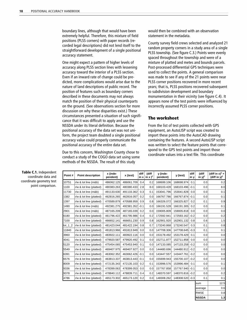
From the list of test points collected with GPSequipment, an AutoLISP script was created toimport these points into the AutoCAD drawingcontaining the features. A second AutoLISP scriptwas written to select the feature points that corre-spond to the GPS test points and import thosecoordinate values into a text file. This coordinate

Point # Point descriptionx (inde-

pendent)x (test)

diffin x

(diffin x ) 2

y (inde-pendent)

y (test)diffin y

(diffin y) 2

(diff in x) 2 +(diff in y) 2

10751 r/w & lot line (m&b) 486062.125 486061.709 0.4 0.2 168699.106 168698.974 0.1 0.0 0.2

1100 r/w & lot line (platted) 480383.263 480380.433 2.8 8.0 168103.428 168103.496 -0.1 0.0 8.0

11730 r/w & lot line (m&b) 491133.630 491133.362 0.3 0.1 153041.796 153041.828 0.0 0.0 0.1


1397 r/w & lot line (platted) 470589.879 470588.959 0.9 0.8 166326.072 166325.827 0.2 0.1 0.9

1490 r/w & lot line (m&b) 492381.275 492381.352 -0.1 0.0 166191.528 166191.305 0.2 0.0 0.1

2901 r/w & lot line (m&b) 487165.209 487165.039 0.2 0.0 159005.809 159005.818 0.0 0.0 0.0



lot_1_2 r/w & lot line (platted) 481423.044 481422.194 0.8 0.7 173240.868 173240.547 0.3 0.1 0.8






6391 r/w & lot line (platted) 463062.352 463062.426 -0.1 0.0 143447.557 143447.761 -0.2 0.0 0.0

6576 r/w & lot line (platted) 463813.337 463813.443 -0.1 0.0 155699.943 155700.107 -0.2 0.0 0.0





sum 12.5

average 0.6

RMSE 0.8

NSSDA 1.3

Table C.1. Independentcoordinate data and

coordinate geometry testpoint comparison.


Point # Point description x (inde-pendent) x (test) diff

in x(diff

in x ) 2y (inde-

pendent) y (test) diffin y (diff in y) 2 (diff in x) 2 +

(diff in y) 2

34 152nd-stream 3 459897.8245 459900.2241 -2 6 254995.3250 254990.1862 5 26 32

35 132nd-Isleton 4 475603.3345 475602.9600 0 0 244363.6045 244371.4900 -8 62 62

36 155th-Manning 5 489350.1000 489350.1700 0 0 256106.3855 256110.1900 -4 14 14

37 180th-Keystone 6 483572.5260 483572.5700 0 0 269361.1230 269357.1800 4 16 16

38 May-RR 7 494171.3170 494160.1307 11 125 238673.6400 238666.0810 8 57 182

40 Otchipwe-94th 9 505295.9165 505293.1600 3 8 223453.3670 223446.1800 7 52 59

41 Neal-BrwnsCr. 10 497444.6805 497461.9147 -17 297 218442.2285 218479.5031 -37 1389 1686

42 75th-Keats 11 481800.0900 481797.1300 3 9 213775.5375 213762.8200 13 162 170

43 Irish-RR 12 475144.8540 475146.2412 -1 2 233082.6265 233082.4062 0 0 2

44 Linc-Robert 13 466236.2490 466238.0000 -2 3 211022.1690 211022.2500 0 0 3

45 C.R. 6-Stream 14 475253.3275 475247.4079 6 35 189933.5615 189931.4246 2 5 40

46 4th-Grd.Ang. 15 472999.8705 473000.8200 -1 1 175394.1410 175391.2300 3 8 9

47 Lake-Century 16 461164.5183 461162.2000 2 5 163210.0978 163207.3600 3 7 13

49 65th-Geneva 18 460948.6040 460948.0200 1 0 140008.1990 140006.2700 2 4 4

50 50th-ditch 19 496582.6795 496567.2195 15 239 147523.4710 147536.9953 -14 183 422

51 Jama-EPDR 20 474434.7155 474434.5700 0 0 126212.9210 126207.5300 5 29 29

52 Pioneer-GCID 21 460963.7915 460964.1100 0 0 118776.1925 118775.1700 1 1 1

53 127th-NB10 22 493944.2820 493949.9100 -6 32 106859.0630 106859.2000 0 0 32

54 Wash-Frontg 23 500142.5240 500140.4300 2 4 206064.7665 206062.9800 2 3 8

55 Point-RR 24 513038.7305 513036.5199 2 5 203149.2675 203144.4737 5 23 28

56 30th-Norman 25 498843.6095 498848.6000 -5 25 189987.0710 189984.8500 2 5 30

57 Rivercrest-Riv 26 516059.2450 516059.0524 0 0 180143.2225 180136.5409 7 45 45

58 Ramp-S.B.15 27 492428.0940 492427.6400 0 0 173572.2310 173557.3200 15 222 223

59 Indian-Hud. 28 500207.7530 500207.0900 1 0 173314.2015 173312.5700 2 3 3

60 VllyCr.-Put. 29 512300.0370 512306.3396 -6 40 162002.5330 162005.9951 -3 12 52

62 87th-Quadrant 30 513787.7670 513805.4900 -18 314 128008.0970 128011.9900 -4 15 329

2 Road-RR 512838.5425 512832.1230 6 41 265305.5275 265304.6426 1 1 42

3 Road-Road 513804.5885 513779.1351 25 648 265288.9815 265292.0679 -3 10 657

4 Road-RR 506995.3440 506986.9698 8 70 259036.2875 259039.1469 -3 8 78

5 Road-Road 505890.0345 505900.1300 -10 102 267608.0790 267586.4100 22 470 571

6 Road-Road 499522.8775 499516.9900 6 35 268070.4880 268057.5600 13 167 202

7 Road-Road 500886.3235 500889.8827 -4 13 277084.7130 277076.8184 8 62 75

9 Road-Road 506832.2160 506832.9800 -1 1 284524.2900 284524.2300 0 0 1

15 Road-Road 512469.9380 512494.5300 -25 605 300556.4700 300550.1500 6 40 645

16 Road-Road 499541.7365 499542.9300 -1 1 295469.7610 295470.3500 -1 0 2

19 Stream-Road 495674.4090 495672.6012 2 3 295158.3380 295155.4875 3 8 11

20 Road-Road 493348.3880 493356.4200 -8 65 283897.9365 283893.6900 4 18 83

21 Road-Road 486511.0920 486512.7100 -2 3 275873.6795 275878.2400 -5 21 23

22 Road-Road 483617.1320 483617.8700 -1 1 275899.2500 275902.5300 -3 11 11

23 Stream-Road 479455.9240 479472.6850 -17 281 291709.0365 291683.7402 25 640 921

24 Road-Road 469037.3285 469025.2000 12 147 298365.8860 298366.1900 0 0 147

25 Road-Road 456160.0730 456172.3500 -12 151 300964.3090 300970.9900 -7 45 195

26 Road-Road 453048.3560 453051.8400 -3 12 300995.9335 301016.3400 -20 416 429

31 Road-Road 471995.9350 472007.9600 -12 145 289610.8105 289606.5200 4 18 163

32 Road-Shoreline 471828.5090 471845.6500 -17 294 289748.0805 289734.9000 13 174 468

33 Stream-Road 473084.1800 473083.8500 0 0 283256.8455 283250.2300 7 44 44

36 Stream-Road 467667.6425 467674.1085 -6 42 272602.0220 272610.5601 -9 73 115

37 Stream-Stream 452112.0170 452108.5500 3 12 277310.9820 277322.2800 -11 128 140

38 Road-Road 451973.4935 451977.1198 -4 13 269628.2735 269625.6395 3 7 20

41 Road-Road 473066.7460 473069.3294 -3 7 264154.8040 264153.7500 1 1 8

sum 8545

average 171

RMSE 13

NSSDA 23

text file was then inserted into the spreadsheettable where calculations could be performed.

For linear features identified in the river valleys,points were selected at regular intervals from boththe GPS control values and the check point dataset. The number of points collected from eachfeature area ranged from four to 22 depending onthe nature of the selected feature. These pointswere fed into an individual spreadsheet template.Two spreadsheet tables are provided as examples(see tables C.1 and C.2).


A preliminary comparison was made of the digi-tized part of this data set. Several divisions of theoverall 50 points were made. Separate spread-sheets comparing each were prepared. Pointsgroupings were: north half of the county; southhalf of the county; 25 of 50 points selected atrandom; and all 50 points. The results were: 25feet, 20 feet, 23 feet and 23 feet, respectively. Thisshows good uniformity.

Table C.2. Independentcoordinate data and

digitized test pointcomparison.


Digitized linear features. Although unique, theresult shown for the special linear features didproduce a result matching estimates developedyears earlier from experience in mapping theseareas. A horizontal error of up to 120 feet can beexpected for the digitized features in the high reliefareas.

COGO features. The method chosen to comparevalues between control and data checkpoints doesnot entirely conform to the NSSDA. Limiting thescope of control to a single township was inten-tional due to the nature of the COGO data set. Forthis reason, the potential cost as compared to thefinal value could not be justified in locating controlcountywide. Apparently by chance, results of thestudy area seem to indicate that none of the 21points selected for control are related to a recov-ered PLSS corner position type. From experience inbuilding the parcel database, the 1.3 foot result(table C.1) meets expectations. This appeared arealistic representation of what exists over most ofthe county in areas not influenced by a correctedsection corner position.


The project team thought it would be useful andinformative for potential data users to better un-derstand the methods used to derive the accuracystatements. The team developed a brief descriptionof the test to fill out the positional accuracy por-

tion of the metadata, in addition to pointing thereader to other sources of information.

In the case of COGO data, the project team be-lieved a specialized summary statement can moreappropriately communicate the positional accuracyof the data than can the accuracy reporting state-ment of the NSSDA. Although this is not as simpleand standardized as the NSSDA statement, thismethod does provide a higher level of informationto the user, hopefully increasing the user’s confi-dence in the data and allowing the data to be usedmore appropriately.


An optional method of collecting COGO controlwas considered but not used by WashingtonCounty, but it may be instructive to others at-tempting to implement the NSSDA.

The county was divided into quadrants. Five pointswere selected within each quadrant. Considerationwas given to areas of greater feature density,occasionally concentrating more points in theseareas. A buffer of 2 miles (the diameter of 4 milesis approximately equal to 10 percent of the diago-nal distance across the data set) was generatedaround each point. The NSSDA calls for a minimumof 20 points. The following types of points weredesignated:

railroad crossing with highway

lot corner in subdivision plat

Figure C.5. Detailedpositional accuracy

statements as reported inmetadata.


Digitized features of the parcel map database outside areas of high vertical relief tested23 feet horizontal accuracy at the 95% confidence level using modified NSSDA testingprocedures. See Section 5 for entity information of digitized feature groups. See alsoLineage portion of Section 2 for additional background. For a complete report of thetesting procedures used contact Washington County Surveyor’s Office as noted in Section6, Distribution Information.

Digitized features of the parcel map database within areas of high vertical relief tested119 feet horizontal accuracy by estimation as described in the complete report notedabove.

All other features are generated by coordinate geometry and are based on a frameworkof accurately located PLSS corners positions used with public information of record.Computed positions of parcel boundaries are not based on individual field survey.Although tests of randomly selected points for comparison may show high accuracybetween field and parcel map content, variations between boundary monumentationand legal descriptions of record can and do exist. Caution is necessary in use of landboundary data shown. Contact the Washington County Surveyor’s Office for moreinformation.


Not applicable.


lot corner (old plat, metes or bounds) based oncertificate of survey

road intersection

road intersection at PLSS corner

intersection of projected right-of-way line androad centerline

radius point on cul-de-sac

road right-of-way limit at B corner

The parcel map was developed one PLSS section ata time. Typically the cartographer relied on thePLSS as the foundation for information created. Asa result, the positioning of points at the sectioncorners and along the outer edges was more reli-able than within the interior. Because of the waysections are normally subdivided, the least reliablemapped parcels were located near the interior ofeach quarter and quarter/quarter section. Expect-ing exterior section points to be the most accurate,the project team focused on interior points toanticipate the worst case accuracy. Corners ofproperty ownership make up an estimated 90percent of the parcel database. For this reason itseemed appropriate to have a proportionate repre-sentation. The allotment of points was defined asfollows:

subdivision plats, 6 points, 30 percent

metes and bounds parcels, 6 points, 30 percent

right-of-way corners, road intersections,railroad/highway intersections, 6 points, 30 percent

PLSS, 2 points, 10 percent

Where possible these three groups were furtherdivided into categories by 50-year intervals, suchas sources from 1850 to 1900; 1900 to 1950; and1950 to 1998. Again, this option was not used, butmay have merit in other situations.

Incorrectly used PLSS corner positions. Thefollowing discussion exemplifies only a singleaspect of why land descriptions do not alwaysmatch their positions on the ground and whatimpact this can have in trying to apply the NSSDA.

Increased activity in the monument maintenance ofthe Public Land Survey System to support GISdevelopment over the past 15 to 30 years hasprovided for a high rate of consistency betweenland parcels and their descriptions of record. Actu-ally older parcels dating back 100 to 150 years arealso quite consistent in comparison of groundposition and written documents of record. Unfortu-nately, inconsistencies do exist. The inconsistenciescome from situations where subdivision plats andmetes and bounds parcels were established basedon an incorrect PLSS corner position. In areas

where an ongoing maintenance program of thePLSS has not existed, the likelihood of this occur-rence is much greater. Where an incorrectlyassumed PLSS position has caused land occupationto be inconsistent with a property description ofpublic record, laws exist that may protect thelandowner and can sometimes help to remedy thesituation. Unfortunately, the legal record is notalways changed. In these areas, statements ofexpected positional accuracy using strict applica-tion of the NSSDA could mislead the digital datauser. More information is required in the metadatato keep the data user properly informed.

A study of PLSS corners. A single PLSS cornercan control the position of parcels in up to fourPLSS sections. This is essentially the limit of poten-tial impact for a single discrepancy in PLSS cornerposition. A study within a single township (36 PLSSsections) randomly selected from within Washing-ton County estimated the frequency of theseoccurrences. Of the 138 PLSS corners in the town-ship, 10 on record had been corrected from apreviously established incorrect position. Thelength of positional adjustment varied from 0.5feet to 34 feet. It is known that at least as manyothers have also existed but clear documentationof their details does not exist. Unfortunately it ispossible that parcel boundaries were establishedon the ground based on these incorrect PLSS posi-tions. The lack of information about the timeperiod in which these incorrect positions were usedfurther complicates the issue. Relative accuracymay be very high in these situations while absoluteaccuracy is significantly less. This situation canseriously affect the validity of applying the NSSDAto a parcel boundary data set.

Mixed meaning of positional accuracy.What do the results mean when random fieldmonumented property corners are chosen for con-trolling position when compared againstWashington County’s method in establishing itsbase map? At every PLSS section corner positionalaccuracy is at its best. Here ground position wasused as the starting base for digitally mapping thelegally recorded documents. As one moves to theinterior of a section, ground position compared tothe legal record may or may not diminish. Mappingthe interior of the section primarily follows more ofa theoretical record. A blind comparison of amapped parcel corner with a randomly selectedcorresponding monumented ground position caneasily be performed. However, a discrepancy doesnot necessarily dictate that the relative positionalaccuracy of the parcel boundary is anything less


than perfect when ground truth is in disagreementwith the legal record.

With legal rights based many times on possession,errors in legal records or flaws in measurementmethods may not actually reduce the accuracy ofoccupied ownership. Laws provide protectionunder certain circumstances. There are legalmechanisms to protect owners within a subdivi-sion, for example, from all having to relocate theirhomes, physical improvements and land bound-aries because an incorrect PLSS corner positionwas involved. When the NSSDA standard is appliedto this situation, solutions to address some of thestandard’s components are not so straightforward.It is difficult to find a control point three or moretimes greater in accuracy than something that istheoretical. When interpretations of law are intro-duced, ambiguity can further cloud the situation.Although difficult to grasp for the nonprofessionalwho is not familiar with land records and surveying

methods, it is vitally important for the commonuser of parcel based land information to have acertain confidence level when making decisionsbased on information from GIS analysis.

General comments. The nature of a parcel dataset presents some unique challenges. The idea ofgrouping data types or features of differing accu-racy, especially if presented to the user as agraphic, can communicate the quantity and loca-tion of error quite effectively (see figure C.6). Asland boundaries have evolved since the mid-1800sin Washington County, so have the measurementmethods. Land settlement and correspondingboundary development have been random butsome consistent patterns may be found. Groups ofaccuracy can perhaps be tied to parcels reflectingtheir original measurement quality — fromGunter’s chain to steel tape to computerized elec-tronics and satellites. Collections of parcels mayowe their associated accuracy to whether theterrain is level or hilly. The added characteristics ofplace in time, or the nebulous facets of law makefor additional complications.

This example project required good familiarity withthe subject data set to properly apply the NSSDAaccording to its specifications. Spatial features ofthe database were known to be of varying accu-racy and were selectively grouped in some cases.In other instances, applying the standard becamedifficult. A standard designed to address the vastrange of GIS data types can, at times, have a “onesize fits all” feeling. To avoid this impression andstill accomplish the task, the underlying intentmust be considered, with reasonable and straight-forward approaches explored and applied. Thiswas the intention when applying the NSSDA to theWashington County parcel base. The major ob-stacles encountered were a result of the nature ofthe features being represented in the parcel baseand the implications of boundary law.

The Washington County project team believes thebest solution is to provide as much information aspossible by meeting metadata standards andshowing thoroughness in critical background infor-mation. The NSSDA can provide important andneeded information, but may not give the completepicture in all applications.

Figure C.6. Digitizedfeatures of Washington

County grouped byaccuracy.

Higher accuracyLower accuracy


Case Study D

The Lawrence GroupDescribing positional accuracy of a street centerline data set when NSSDA testing cannot be applied

The project

Although the intent was to use the NationalStandard for Spatial Data Accuracy to describe,measure and report the positional accuracy of aregional street centerline data set, the LawrenceGroup was unable to implement the NSSDA due totime and budget constraints. This modified project,however, is a good example of how to report use-ful information about positional accuracy, evenwhen NSSDA testing is not applied.

The tested data set

The Lawrence Group Street Centerline Database isa digital network of pavement and road right-of-waycenterlines covering the Twin Cities metropolitanarea. The seven-county regional data set consistsof approximately 140,000 graphic elements as wellas associated attribute information. It is generallycreated in state plane coordinates and provided tousers in UTM coordinates. As is typical of regionaldata sets, the positional source documents used forits creation were numerous and varied in quality.

The initial centerline data set was created over aperiod of several years. During the last decade, avariety of additional sources of information havebecome available. Rather than using only hardcopyreferences such as half-section and plat maps,sources such as digital parcel base maps, digitalorthophotos, global positioning references, en-hanced control points and satellite imagery havebecome increasingly accessible. The variety ofreference sources used is also due to the limitedavailability of certain source materials. For example,some counties have completed highly accuratedigital source material, while other counties havenot. Generally, the quality of source material hasimproved, as evidenced by the increasing availabil-ity of high resolution digital ortho imagery.


Several issues arose in the attempt to choose inde-pendent points applicable to a regional street

centerline file. It was necessary to find controlpoints that were known to be more accurate andto permit the data set to be tested at numerous,ideally random locations and to have point loca-tions that could be identified on the streetcenterlines data set.

Since this regional data set was developed from avariety of sources, it was also necessary to have anunderstanding of the accuracy and availability ofpotential independent data sets in different partsof the region.

Evaluating existing independent data sets.If Public Land Survey corners were to be used, theywould have to be associated with street centerlines.This may be possible at street intersections that lieat survey corners. However, this would essentiallyeliminate the random selection of control points,and force accuracy measurement only at intersec-tions that are typically reliable and well established.

Since Public Land Survey corners were unable toprovide a random and unbiased sampling, otherindependent reference points with reference infor-mation pertaining to the streets or street centerlineswere needed. The Lawrence Group found such aset of information through the Minnesota Depart-ment of Transportation in the form of county mapsshowing various control marks as determined bydifferent organizations. These marks are numberedand, although they do not provide for a randomselection of measurable points, there were suffi-cient corresponding coordinate information andstreet centerline tie descriptions to develop a rea-sonable sampling of measurement locations.Unfortunately, it was determined that using thesedescriptive ties to reference the streets was insuffi-cient for establishing a set of points that meetNSSDA requirements due to the potential marginof error in the descriptive variables.

Without a suitable independent data set, the onlyoption to establish a new set of control points wasby means of global positioning devices. Unfortu-nately, The Lawrence Group did not have the stafftime, expertise, equipment and budget needed to

PROJECT TEAM

Jim MaxwellVice president, GISservices

Dan OchGIS specialist


collect such a data set. The result is that the dataset remains untested using the NSSDA.

Providing other positional accuracy infor-mation. If fewer than 20 test points are available,the NSSDA recommends three alternatives fordetermining positional accuracy as described inanother FGDC standard — the Spatial Data Trans-fer Standard. They are: 1) deductive estimate, 2)internal evidence and 3) comparison to source. Inthis case, a significant amount of internal evidenceis available and should be provided in the metadata.

The worksheet

Not applicable for reasons specified above.


Not applicable for reasons specified above.


See figure D.1. for an example of how a descriptivemetadata record can be presented when NSSDAtesting is not applied.


While the Global Positioning System option forcollecting independent data is an excellent meansof providing a positional accuracy measuring solu-tion, some practical obstacles should be noted.First, high quality GPS equipment is costly and notalways available to the data provider. Second, theequipment and associated base station utilizationrequires expertise. Third, this method requiressignificant staff hours since base stations need tobe attended and GPS receivers require a techni-cian. The effort could require four to seven peopleto coordinate a project of this size.

Overcoming these obstacles may be difficult. Formany organizations, funds and expertise are notreadily available. It may require a coordinatedeffort by any or all parties with an interest in thepositional accuracy of the data set. The coordi-nated effort may require the sharing of costs, staffand expertise. However, if these obstacles areovercome, this option can be an excellent methodfor measuring and conforming to NSSDA guidelines.

Figure D.1. Detailedpositional accuracy

statements as reported inmetadata.


There are differing degrees of positional accuracy throughout the centerline data set.Positional accuracy of the data is adjusted to available sources known to have greaterdegrees of accuracy than those used to generate the existing data. However, in all cases(including instances where COGO line work has been the reference) street segments weregeneralized to at least 4 feet in order to reduce the number of vertices, thus reducing file size.

The goal is to have 95% of roads located to within the digital right-of-way or pavementcenterlines provided from counties, where such digital data is available. In other areas, 95%of roads are intended to be within ten meters of the road or right-of-way center.

The centerlines of Dakota and Washington counties were adjusted by referencing theWashington and Dakota County Surveyors department geospatial data set. Positionaladjustments were also made to data supplied by the Ramsey County Public Worksdepartment in May 1998. These adjustments were made relative to each county’s centerlinedata set. Ramsey County was continuing to review its own data for positional accuracy;however, adjustment was necessary in order that users could more efficiently use both datasets concurrently. Due to the large number of changes, the Ramsey County adjustments arenoted here in the metadata rather than being reflected in the quarterly change report asindividual segment changes.

Positional adjustments were made as of July 31, 1998 to street centerlines within the city ofMinneapolis. These changes were made relative to street centerlines provided by the city ofMinneapolis. Due to the large number of changes, these positional adjustments are notedhere rather than in the quarterly change report.

For all other areas, various resources were used. For more information please review the“Lineage” section of this metadata record.


Not applicable.


The project

The objective was to explore whether or not it isreasonable to develop positional accuracy assess-ments of height-of-land watershed delineations.Unlike parcel corners, township survey monumentsand other similar features, it is conceptually difficultto meaningfully evaluate watershed delineationsfor positional accuracy. Professionals use detailedtopographic maps and expertise to locate height-of-land boundaries for watersheds or drainagebasins. In the end, what matters most is not thepositional accuracy of individual points, but theoverall fidelity a watershed delineation has withfield experience regarding how a particular drain-age basin actually functions.

However, since the state has a growing number ofwatershed delineations, from the major basin ondown to lake- and ditch-shed, positional accuracyassessments might be useful as a way to evaluatethe suitability of a particular delineation for a par-ticular task. For example, the DNR was requested toprovide a reasonably accurate delineation of theRed River of the North regional drainage for use ina climatological modeling project.

Figure E.1. NSSDA majorwatershed sample points

Case Study E

Minnesota Department of Natural ResourcesAttempting to apply the NSSDA to a statewide watershed data set containing nondiscrete boundaries

PROJECT TEAM

Glenn RaddeWetlands GIS manager

Joe GibsonIS manager, Departmentof Natural Resources,Waters

Jim SolstadSurface water hydrologist,Department of NaturalResources, Waters

The most detailed data covers only Minnesota,with access to national Hydrologic Unit Code dataof drainage basins at two scales: 1:250,000 and1:2 million. A positional accuracy assessmentmight help clarify the use of these smaller scalecoverages for more detailed studies. This projectestablished sample points to compare the posi-tional accuracy of these small scale coverages tothe more detailed statewide coverage DNR Watershas developed in cooperation with various stateand federal agencies.

The tested data set

The project team tested the positional accuracy ofthe U.S. Geological Survey 1:250,000 and 1:2million Hydrologic Unit Code data sets. Both ofthese national data sets were derived from1:500,000 and 1:250,000 source maps during the1970s. Since these coverages are readily availableon the Internet, they remain authoritative, nationaldelineations. For this purpose, the federal eight-digit Hydrologic Unit Codes correspond toMinnesota’s major and minor watershed identi-fication numbers. These evaluations focused oncomparing the delineations of major watershedswith the corresponding eight-digit HUCs.


The project team used the /basins95 coverage asan independent data set of higher accuracy. The /basins95 coverage was first created in 1977 bymanually delineating height-of-land watersheds of5-6 square miles in area on USGS 7.5-minute quad-rangles. In the early 1990s, these mylars wereassembled and scanned as 1:100,000-scale mapsheets. A diverse group, including state and federalagencies and Mankato State University, worked onverifying and correcting known errors in this dataset. In 1993, the Department of Natural Resourcesincorporated major and minor drainage basin data,at 1:24,000-scale, from both the USGS for theMinnesota River Basin and Mankato State Univer-sity Water Resources Center for its 13-county

NSSDA samplesBasins95 base data


Best Ten Sample PointsID X-Coord Y-Coord X-Diff Y-Diff Squared/Summed

58 316246 5194439 22 16 740

9 515466 4954879 104 -27 11545

35 327887 5257696 -62 -106 15080

70 450940 4990434 -125 0 15625

63 489464 5061367 116 58 16820

80 322470 5057799 -148 42 23668

20 248112 4891460 27 -161 26650

71 438771 4973151 -177 0 31329

15 337579 5372432 69 -180 37161

16 337578 5372430 68 -183 38113

Worst Ten Sample PointsID X-Coord Y-Coord X-Diff Y-Diff Squared/Summed

76 473392 4853699 2325 3452 17321929

77 470152 4848275 4438 2254 24776360

25 363075 4945478 2414 -5375 34718021

47 389175 5126315 4196 4416 37107472

61 484658 5136228 1198 -6197 39838013

13 564580 5292404 -5981 -3006 44808397

18 282652 4841907 -1668 6740 48209824

55 313005 5233367 -6482 2672 49155908

39 423720 5198685 -5635 5153 58306634

64 485839 5023201 1794 7600 60978436

SUM 631,448,624

AVG 7,700,592.98

RMSE 2,774.99

NSSDA 4,802.96

Best Ten Sample PointsID X-Coor Y-Coord X-Diff Y-Diff Squared/Summed

66 408186 5049328 -8 -13 233

58 316246 5194439 409 -58 170,645

15 337579 5372432 409 -108 178,945

16 337578 5372430 409 -112 179,825

8 523951 4917059 -77 -473 229,658

9 515466 4954879 393 -285 235,674

51 459012 5261312 498 -231 301,365

69 459036 5010406 -241 -494 302,117

23 325843 4923739 70 -575 335,525

5 529633 4829235 143 -664 461,345

Worst Ten Sample PointsID X-Coord Y-Coord X-Diff Y-Diff Squared/Summed

54 527131 5267895 -4166 -570 17,680,456

37 326526 5311468 -122 4268 18,230,708

24 349658 4953280 -4489 1653 22,883,530

18 282652 4841907 -1387 5143 28,374,218

47 389175 5126315 4172 3928 32,834,768

13 564580 5292404 -5292 -3006 37,041,300

61 484658 5136228 1372 -7048 51,556,688

64 485839 5023201 2005 7785 64,626,250

55 313005 5233367 -8810 2923 86,160,029

39 423720 5198685 -6918 6395 88,754,749

SUM 703,400,916

AVG 8.578,059.95

RMSE 2,928.83

NSSDA 5,069.22

Table E.1 (left).Comparing 1:250,000

HUC to DNR’s 1995basins; 10 best and worst

sample points.

Table E.2 (right).Comparing 1:2 million

HUC to DNR’s 1995basins; 10 best and worst

sample points.

service area in southwestern Minnesota. The resultof these efforts has been the creation of the mostauthoritative and comprehensive data set of drain-age basins for Minnesota.

It is important to note that there are discrepanciesbetween the three data sets discussed here. Forexample, the /basins95 coverage contains delinea-tions of 81 major watersheds, ranging from 12.54square miles in size to 2,852.87 square miles. TheUSGS 1:250,000-scale HUC coverage delineates 82major drainage basins ranging from 6.14 squaremiles to 2,885.94 square miles. Finally, the USGS1:2 million-scale HUC coverage delineates 86major drainage areas ranging in size from 16.08square miles to 2,927.15 square miles, with somesliver polygons of 0.03 square miles.

The worksheet

Figure E.1 shows the location of 82 sample pointsfrom which to compare each of the three drainagebasin delineations. The project team selected out-lets, pour points or other edge or boundaryfeatures that provided clean sample points repre-senting the intersection of one major watershed

with another. The team thought that a positionalaccuracy assessment of these points would providea reasonable comparison between the three cover-ages.

Tables E.1 and E.2 show the results of the compari-sons. The table evaluating all 82 sample pointsacross the three coverages is quite lengthy, so the10 best and worst sample points are presentedbased on how they ranked as squared andsummed differences.


The NSSDA statistic for the 1:250,000-scale HUCcoverage evaluated against the /basins95 data is4,802.96 meters (or 4.8 kilometers), and the 1:2million-scale HUC coverage statistics is 5,069.22meters (or 5.1 kilometers). When the project teamcompared the 1:2 million-scale HUC coverageagainst the more detailed 1:250,000-scale HUCdata, the resulting NSSDA statistic was 3,785.50meters (or 3.8 kilometers).

While these numbers may seem large, the posi-tional accuracy reported here does not preclude a


number of valid uses of the data sets, as discussedin the observations section.


Figure E.2 contains formal NSSDA reports for both1:250,000-scale and 1:2 million-scale HUC data sets.


At first glance, it may appear that things are notall that well between the three height-of-landdelineations of Minnesota’s major watersheds.Federal efforts were begun and finished long be-fore Minnesota did any of its more detailedstudies. Minnesota has subsequently revised this

more detailed data, and is currently cooperativelyworking on adding lakeshed delineations to thedrainage basin hierarchy.

This small study does demonstrate the process ofidentifying, calculating and reporting positionalaccuracy statistics for watershed pour points, out-lets and similar features. Most importantly, itvalidates that these smaller scale coverages stillhave value. The largest NSSDA statistic wasslightly greater than 5 kilometers, which was wellwithin the climatology project’s 10 kilometer accu-racy requirement. While any of these coverageswould have worked well, the NSSDA statistic doesprovide useful insights as to when it is wise to uselarger-scale data.

Figure E.2. Positionalaccuracy statements as

reported in metadata.Horizontalpositionalaccuracy

Using the National Standard for Spatial Data Accuracy, the 1:250,000-scale HUC data tested4,802.96 meters horizontal accuracy at 95% confidence level.

Using the National Standard for Spatial Data Accuracy, the 1:2 million-scale HUC data tested5,069.22 meters horizontal accuracy at 95% confidence level.


Not applicable.


Appendix

National Map Accuracy Standards

In 1941, the U.S. Bureau of the Budget (now theOffice of Management and Budget) developedpositional accuracy specifications for federal mapsknown as the United States National Map Accu-racy Standards. Although revised periodically, thestandards are still in use today.

The standards were written for published papermaps at a time long before digital spatial data.Accuracy testing was generally applied to a mapseries by federal agencies using representativesampling. Positional accuracy in this and otherstandards is defined by two components: horizontalaccuracy and vertical accuracy. Horizontal accuracyis determined by map scale. A threshold was es-tablished for maps with a published scale larger orsmaller than 1:20,000. For maps with scales largerthan 1:20,000, not more than 10 percent of thepoints tested can be in error by more than 1/30 inch.For maps with publication scales of 1:20,000 orsmaller, the error distance decreases to 1/50 inch.

This standard relies upon testing of “well-definedpoints.” Selected points identifiable on both themap and on the ground are measured and thedifference between the two — the error betweenmapped and actual location — is recorded in mapinches at the publication scale. Standards for atypical 1:24,000-scale U.S. Geological Survey quad-rangle is 40 feet, or 1/50 inch at map scale. Thestatistic used is based on a 90 percent confidencelevel; 90 percent of the tested points must fallwithin the standard’s threshold to comply.

Vertical accuracy involves a methodology similar tothat used in horizontal accuracy testing. The verti-

cal testing also references map publication scaleand involves a 90 percent threshold regardingnumber of test points required. At all map scales,the maximum allowable vertical tolerance is one-half the published contour interval.

National Map Accuracy Standards do not requireany description of the testing process to determinemap accuracy. The standard does note that “sur-veys of higher accuracy” may be used for testingpurposes. It is generally assumed that surveys ofhigher accuracy are acquired independently, al-though no specific criteria are provided.

In summary, general characteristics of the NationalMap Accuracy Standards include positional accu-racy testing that is largely dependent on mappublication scale with test results of selectedpoints reported in inches at map scale. The stan-dards specify that 90 percent of the well-definedpoints tested must fall within a specified tolerancebased on the map publication scale. If the mapmeets accuracy standard requirements it can belabeled as complying with National Map AccuracyStandards.

Another map accuracy standard of potential inter-est, but not discussed in this handbook, is theAmerican Society for Photogrammetry and RemoteSensing Accuracy Standards for Large-Scale Maps.These accuracy standards address both horizontaland vertical accuracy, allow for multiple “classes”of map accuracy, and provide specific detail re-garding map accuracy testing requirements.Several aspects of these standards are included inNSSDA and referenced in that document.


UNITED STATES NATIONAL MAP ACCURACY STANDARDS

With a view to the utmost economy and expedition in producing maps which fulfill not only the broad needs forstandard or principal maps, but also the reasonable particular needs of individual agencies, standards ofaccuracy for published maps are defined as follows:

1. Horizontal Accuracy. For maps on publication scales larger than 1:20,000, not more than 10 percent ofthe points tested shall be in error by more than 1/30 inch, measured on the publication scale; for maps onpublication scales of 1:20,000 or smaller, 1/50 inch. These limits of accuracy shall apply in all cases to positionsof well- defined points only. Well-defined points are those that are easily visible or recoverable on the ground,such as the following: monuments or markers, such as bench marks, property boundary monuments,intersections of roads, railroads, etc.; corners of large buildings or structures (or center points of smallbuildings); etc. In general what is well defined will also be determined by what is plottable on the scale of themap with 1/100 inch. Thus while the intersection of two road or property lines meeting at right angles wouldcome within a sensible interpretation, identification of the intersection of such lines meeting at an acute anglewould obviously not be practicable within 1/100 inch. Similarly, features not identifiable upon the groundwithin close limits are not to be considered as test points within the limits quoted, even though their positionsmay be scaled closely upon the map. In this class would come timber lines, soil boundaries, etc.

2. Vertical Accuracy, as applied to contour maps on all publication scales, shall be such that not more than10 percent of the elevations tested shall be in error more than one-half the contour interval. In checkingelevations taken from the map, the apparent vertical error may be decreased by assuming a horizontaldisplacement within the permissible horizontal error for a map of that scale.

3. The accuracy of any map may be tested by comparing the positions of points whose locations orelevations are shown upon it with corresponding positions as determined by surveys of a higher accuracy. Testsshall be made by the producing agency, which shall also determine which of its maps are to be tested, and theextent of such testing.

4. Published maps meeting these accuracy requirements shall note this fact on their legends, asfollows: “This map complies with National Map Accuracy Standards.”

5. Published maps whose errors exceed those aforestated shall omit from their legends all mention ofstandard accuracy.

6. When a published map is a considerable enlargement of a map drawing (manuscript) or of apublished map, that fact shall be stated in the legend. For example, “This map is an enlargement of a 1:20,000-scale map drawing,” or “This map is an enlargement of a 1:24,000-scale published map.”

7. To facilitate ready interchange and use of basic information for map construction among allfederal map making agencies, manuscript maps and published maps, wherever economically feasible andconsistent with the uses to which the map is to be put, shall conform to latitude and longitude boundaries,being 15 minutes of latitude and longitude, or 7.5 minutes or 3-3/4 minutes in size.

US Bureau of the Budget

Issued June 10, 1941Revised April 26, 1943Revised June 17, 1947

positional accuracy handbook - mn it services

Documents