position locationing for millimeter wave systems
TRANSCRIPT
Position Locationing for Millimeter Wave Systems
Ojas Kanhere, Theodore S. RappaportNYU WIRELESS
NYU Tandon School of Engineering
Brooklyn, NY 11201
{ojask,tsr}@nyu.edu
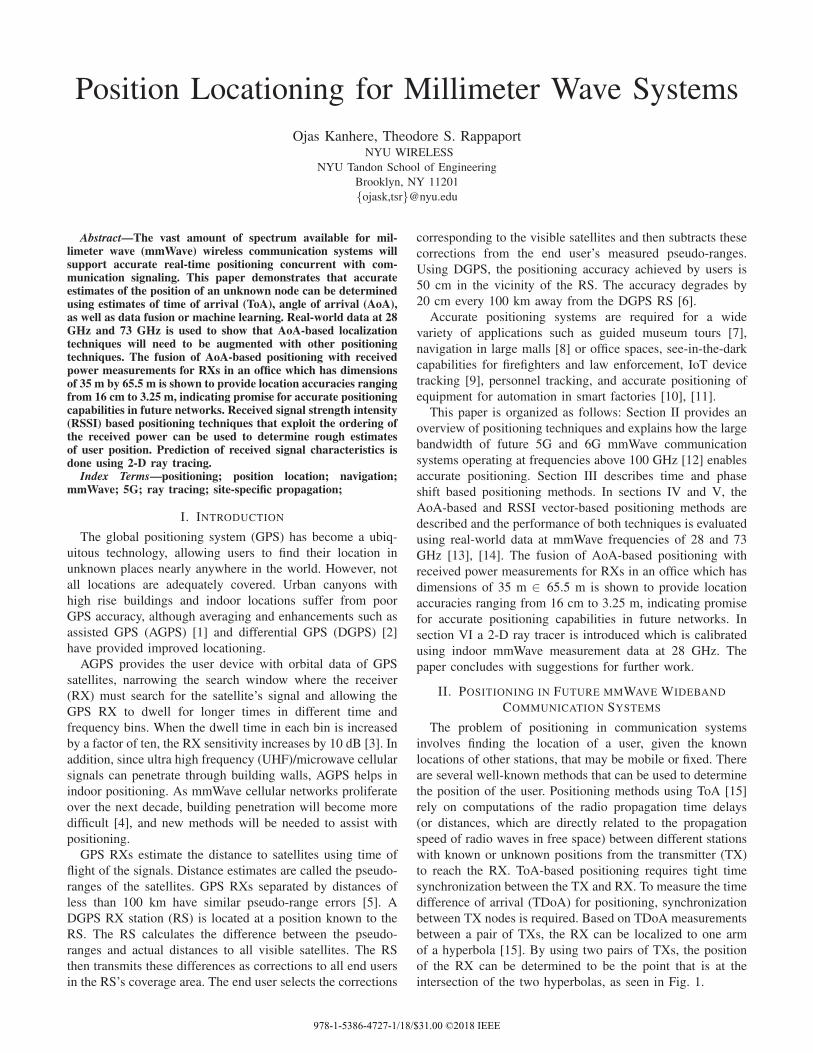
Abstract—The vast amount of spectrum available for mil-limeter wave (mmWave) wireless communication systems willsupport accurate real-time positioning concurrent with com-munication signaling. This paper demonstrates that accurateestimates of the position of an unknown node can be determinedusing estimates of time of arrival (ToA), angle of arrival (AoA),as well as data fusion or machine learning. Real-world data at 28GHz and 73 GHz is used to show that AoA-based localizationtechniques will need to be augmented with other positioningtechniques. The fusion of AoA-based positioning with receivedpower measurements for RXs in an office which has dimensionsof 35 m by 65.5 m is shown to provide location accuracies rangingfrom 16 cm to 3.25 m, indicating promise for accurate positioningcapabilities in future networks. Received signal strength intensity(RSSI) based positioning techniques that exploit the ordering ofthe received power can be used to determine rough estimatesof user position. Prediction of received signal characteristics isdone using 2-D ray tracing.
Index Terms—positioning; position location; navigation;mmWave; 5G; ray tracing; site-specific propagation;
I. INTRODUCTION
The global positioning system (GPS) has become a ubiq-
uitous technology, allowing users to find their location in
unknown places nearly anywhere in the world. However, not
all locations are adequately covered. Urban canyons with
high rise buildings and indoor locations suffer from poor
GPS accuracy, although averaging and enhancements such as
assisted GPS (AGPS) [1] and differential GPS (DGPS) [2]
have provided improved locationing.
AGPS provides the user device with orbital data of GPS
satellites, narrowing the search window where the receiver
(RX) must search for the satellite’s signal and allowing the
GPS RX to dwell for longer times in different time and
frequency bins. When the dwell time in each bin is increased
by a factor of ten, the RX sensitivity increases by 10 dB [3]. In
addition, since ultra high frequency (UHF)/microwave cellular
signals can penetrate through building walls, AGPS helps in
indoor positioning. As mmWave cellular networks proliferate
over the next decade, building penetration will become more
difficult [4], and new methods will be needed to assist with
positioning.
GPS RXs estimate the distance to satellites using time of
flight of the signals. Distance estimates are called the pseudo-
ranges of the satellites. GPS RXs separated by distances of
less than 100 km have similar pseudo-range errors [5]. A
DGPS RX station (RS) is located at a position known to the
RS. The RS calculates the difference between the pseudo-
ranges and actual distances to all visible satellites. The RS
then transmits these differences as corrections to all end users
in the RS’s coverage area. The end user selects the corrections
corresponding to the visible satellites and then subtracts these
corrections from the end user’s measured pseudo-ranges.
Using DGPS, the positioning accuracy achieved by users is
50 cm in the vicinity of the RS. The accuracy degrades by
20 cm every 100 km away from the DGPS RS [6].
Accurate positioning systems are required for a wide
variety of applications such as guided museum tours [7],
navigation in large malls [8] or office spaces, see-in-the-dark
capabilities for firefighters and law enforcement, IoT device
tracking [9], personnel tracking, and accurate positioning of
equipment for automation in smart factories [10], [11].
This paper is organized as follows: Section II provides an
overview of positioning techniques and explains how the large
bandwidth of future 5G and 6G mmWave communication
systems operating at frequencies above 100 GHz [12] enables
accurate positioning. Section III describes time and phase
shift based positioning methods. In sections IV and V, the
AoA-based and RSSI vector-based positioning methods are
described and the performance of both techniques is evaluated
using real-world data at mmWave frequencies of 28 and 73
GHz [13], [14]. The fusion of AoA-based positioning with
received power measurements for RXs in an office which has
dimensions of 35 m ∈ 65.5 m is shown to provide location
accuracies ranging from 16 cm to 3.25 m, indicating promise
for accurate positioning capabilities in future networks. In
section VI a 2-D ray tracer is introduced which is calibrated
using indoor mmWave measurement data at 28 GHz. The
paper concludes with suggestions for further work.
II. POSITIONING IN FUTURE MMWAVE WIDEBAND
COMMUNICATION SYSTEMS
The problem of positioning in communication systems
involves finding the location of a user, given the known
locations of other stations, that may be mobile or fixed. There
are several well-known methods that can be used to determine
the position of the user. Positioning methods using ToA [15]
rely on computations of the radio propagation time delays
(or distances, which are directly related to the propagation
speed of radio waves in free space) between different stations
with known or unknown positions from the transmitter (TX)
to reach the RX. ToA-based positioning requires tight time
synchronization between the TX and RX. To measure the time
difference of arrival (TDoA) for positioning, synchronization
between TX nodes is required. Based on TDoA measurements
between a pair of TXs, the RX can be localized to one arm
of a hyperbola [15]. By using two pairs of TXs, the position
of the RX can be determined to be the point that is at the
intersection of the two hyperbolas, as seen in Fig. 1.
978-1-5386-4727-1/18/$31.00 ©2018 IEEE

AoA-based positioning techniques estimate the line of
bearing based on the spatial directional received power at the
RX, and is well suited for narrow beam steerable antennas
that can scan to find the AoAs of three or more sources
with known locations (the “three point problem”) [16]. Using
geometric principles, the line of bearing to multiple TXs
are used to localize the RX [15], [16] using knowledge of
the RX AoAs from various beacons. AoA-based positioning
was proven effective in factory environments for autonomous
vehicles that used a scanning optical RX [16].
Using RSSI-based positioning approaches, the RX can
be positioned, since RSSI generally monotonically decreases
with distance [17]. The RSSI can be determined for a known
environment (e.g. a building) using pre-measured signal
strengths and known TX locations over a grid of locations
(e.g. a map of the environment) from multiple TXs. By
applying a suitable path loss model or pre-measured values
over a grid of locations, with fine enough resolution to offer
the desired accuracy in positioning, the distance between the
TX and RX can be estimated [17]. For many different TXs
with known locations, the resulting position is estimated based
on the best fit, e.g. the most likely location that best matches
all measured signal levels from the multiple TXs [18].
The mmWave regime offers much wider bandwidths than
has ever been available to mobile networks [19], thus offering
both lower latency, and a built-in position location capability
due to the massive transmission bandwidth. A passband
signal with bandwidth B Hz that is sampled at its Nyquist
rate must be sampled every 1/B seconds at baseband. The
raw resolution of mmWave systems, defined as the distance
light travels between these sampling instants, is the smallest
distance difference that can be measured. With available
bandwidth B, the raw resolution is given by [20]:
r =c
B, (1)
where r is the raw resolution in meters, c is the speed of light
in meters per second.
The raw resolution of mmWave systems is much smaller
than the resolution of systems operating at sub-6 GHz fre-
quencies owing to the much greater bandwidths available.
LTE systems use the position reference signal (PRS) for
positioning, which is a pseudo-random sequence sent by LTE
base stations [21]. The 20 MHz 4G LTE channel can use a
PRS that has a bandwidth of at most 20 MHz [21] and thus
has a raw resolution of 15 m. A 4 GHz bandwidth mmWave
or Terahertz (THz) channel could provide a raw resolution
of 7.5 cm. Better accuracy could be obtained by fusing ToA
with accurate AoA information, available due to the narrow
beamwidths of mmWave antennas, and RSSI.
III. TIME AND PHASE BASED LOCALIZATION METHODS
An anchor node is a node whose position is known by
the user. Since electromagnetic waves propagate at the speed
of light, the one-way (e.g. from anchor to user) propagation
Fig. 1. The UE is located at a point that is at the intersection of the arms ofhyperbolas with foci at anchor nodes (F1, F2) and (F1, F3), that correspondto a difference in distance of k. UE′ lies on the arm of the hyperbolacorresponding to a difference in distance of −k [15].
Fig. 2. The UE is in range of several anchor nodes (TXs), which haveknown coordinates. The UE’s coordinates are determined from differentcharacteristics of the signals that arrive at the user from the anchor nodes.
time can be used to estimate the distance of the user from an
anchor node using the relation:
d = c ∈ t, (2)
where d is the estimated distance of the user from the anchor
node and t is the one-way propagation time.
To make the distance estimate accurate, tight synchroniza-
tion between the user and the anchor node is necessary.
Nanosecond-level timing synchronization is required for sub-
meter accuracy, which is costly and increases the system
complexity.
Simpler systems that do not need synchronization can be
designed which measure roundtrip propagation time instead
[22]. The user and the anchor node estimate their signal
processing time, which is then be calibrated out to give the
round-trip time equal to twice the one-way propagation time.
The TDoA method determines the location of the user
relative to the anchor nodes by measuring the difference in
arrival times of signals from the anchor nodes. By measuring
the difference in the ToA of signals from two pairs of anchor
nodes, the difference in distance can be calculated using
(2). If the difference in distance of the user equipment
(UE) from two anchor nodes, F1 and F2, is fixed, i.e. if
dUE F 1 dUE F 2 = k, the locus of the UE is one arm
of a hyperbola with foci at F1 and F2 (the other arm of the
hyperbola corresponds to when the difference is k, as seen
in Fig. 1). The location of the user is the point that is at the
intersection of the two hyperbolas, as seen in Fig. 1.
The cross-correlation of two received signals can be used
to measure the TDoA. The delay that maximizes the cross-
correlation function is the TDoA [15].
A linear frequency modulated (LFM) signal, also called
a chirp signal, has an instantaneous frequency which varies
linearly with time over the chirp duration Tc. These signals
can be used to estimate the TDoA [23], [24]. At the RX,
received signals from two TXs are mixed and then passed
through a low pass filter to give a low frequency signal r(t).The instantaneous frequency of r(t) is proportionate to the
TDoA of the two received signals [23]. Thus, the problem of
estimating the TDoA reduces to estimating the instantaneous
frequency of r(t).An estimate of the phase accrued in the received signal can
also be used to position the RX. The phase of the complex
wireless channel, ∠h, is 2π periodic. For the RX locations
with ToAs that differ by integral multiples of 1/f , ∠h is
the same. The ToA of an RX can be resolved up to an
integral multiple of 1/f . This ambiguity can be resolved by
taking measurements at multiple frequencies, f1, f2, ..., fn,
in which case the ToA of an RX can be resolved up to
an integral multiple of the least common multiple (LCM) of
(1/f1, 1/f2, ..., 1/fn) [25].
IV. AOA-BASED LOCALIZATION
A mobile user can be located using the AoAs of signals
from a set of anchor nodes. The position can be determined
to be the point that is at the intersection of the line of bearing
from the anchor nodes to the user. Two such lines of bearing
are sufficient to determine the location of the user.
Ideally, in noise-free environments, all lines of bearing
would intersect at a single point. However, due to measure-
ment errors and system noise, this is practically never the
case when there are more than two lines of bearing [16]. The
user’s location can then be estimated to be the least square
solution for the intersection of the lines.
To determine the AoAs of the signal from each anchor
node, the user’s antenna should be mechanically or electrically
rotated, until the signal with maximum power is received [26].
In mmWave systems, this direction can be determined during
initial access [27] or in various antenna search or handoff
methods likely to evolve as part of standards that incorporate
directional antennas [26].
A. Accuracy of AoA-Based Positioning for indoor mmWavesystems
To investigate the accuracy of various position location
methods, measured data from a 2014 measurement campaign
at 28 and 73 GHz, at the NYU WIRELESS research center
[13] was used. See Fig. 3(a) for the indoor environment. A
400 Megachip-per-second (Mcps) wideband sliding correlator
channel sounder with high-gain steerable antennas was used
to measure the propagation channel. Five TX and 33 RX
locations were chosen for a total of 48 TX-RX pairs. Out
of the 33 RX locations, 11 were in the range of at least two
TXs (only RX 16 was in the range of three TXs).
Six AoA sweeps and two angle of departure (AoD) sweeps
were conducted at each RX location. The lines of bearing
TABLE I. TX locations used to transmit to each indoor RX location [13].
RX Location Serving TX Locations
1 1
4 1
7 1
8 1, 5
10 2
11 2, 4
12 2, 4
13 2, 4
16 2, 3, 4
18 2, 4
28 4, 5
TABLE II. TX locations used to transmit to each outdoor RX location [14].
RX Location Serving TX Locations
L1 L3, L4, L7, L11, L13
L2 L3, L9, L12
L4 L1, L3, L7, L10, L13
L7 L1, L2, L4, L10
L8 L1, L7, L9
L9 L1, L2, L4, L11
L10 L4, L7, L13
L12 L1, L2, L4, L7, L11
L13 L1, L4, L10
of the TX locations were determined to be the azimuth
directions with maximal received power. The angular sweeps
were centered around the angle at which maximum power was
received, allowing lines of bearing to be measured to within
one degree (the step size of the gimbal). Sweeps were done
in increments of the half power beam width (HPBW) of the
antennas which was 15 at 28 GHz and 30 at 73 GHz. The
power delay profile (PDP) was recorded by time-averaging
20 consecutive PDPs [13].
It was observed that for RXs in NLOS environments, the
strongest arriving beam was not the direct beam. Strong re-
flections were observed off walls and metallic surfaces. Hence
the AoA-based method could not be applied to accurately
localize such nodes. RX 8, 11, 13, 18 and 28 were in LOS of
one TX. The TXs for each RX are listed in Table I. The mean
positioning error for the five LOS nodes was found to be poor:
11.01 m at 28 GHz and 6.20 m at 73 GHz, due to the absence
of two LOS TXs. Accurate positioning could be done if the
locations of the reflections, themselves, were ascertained by
the RX, when a map of the environment is available [28]. This
could be done through ray tracing as described in section VI.
Alternatively, angular information could be used for machine
learning based fingerprinting, as described in section IV-C.
The AoA-based positioning algorithm [15] was also tested
on outdoor propagation data. In the summer of 2016, an
outdoor measurement campaign was conducted on the NYU
Tandon campus in Brooklyn, New York in an open-square
(O.S.) environment, to study base station diversity [14]. Mea-
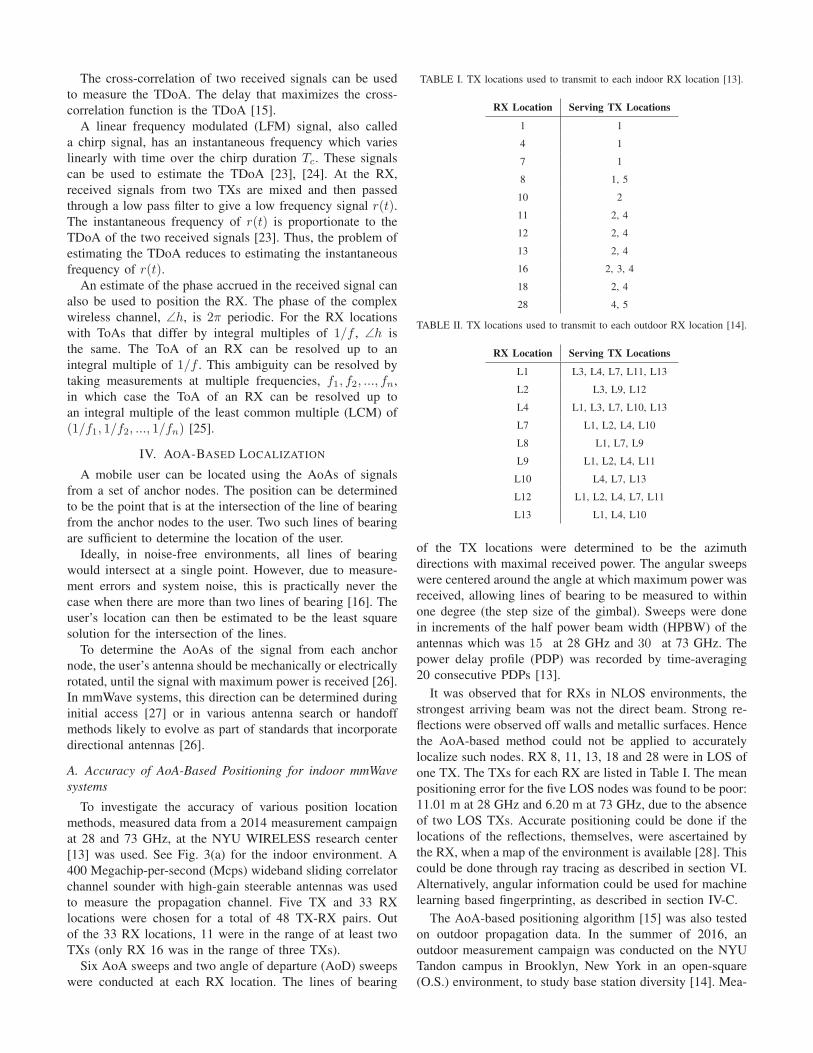
(a) Map of the 9th floor of 2 MTC showing the TX and RX locations where theindoor measurements were conducted at 28 GHz and 73 GHz [13]. The blue linesshow the propagation paths predicted by 2D ray tracing, from TX 1 to RX 6.
(b) The TX and RX locations for the outdoor basestation diversity propagation measurements at 73GHz [14].
Fig. 3. Maps of the indoor and outdoor environments where the AoA-based positioning technique [15] was tested.
surements of the outdoor propagation channel were conducted
at 73 GHz using a 500 Mcps wideband sliding correlator
channel sounder with high-gain steerable antennas. Nine RX
locations were in the coverage area of three to five TXs. The
TXs for each RX are listed in Table II. Of these nine RX
locations, the positioning error at RX 1, 8, 9, 12, and 13 was
less than 40 m, but not particularly good due to absence of
true LOS environments at each RX.
B. Combining AoA and Path Loss Information for GreaterAccuracy
The low accuracy of the AoA-based positioning method
suggests that in mmWave systems, the AoA of strongest
received signal does not necessarily correspond to the AoA
of the LOS signal. In order to achieve better accuracy, we
considered a fusion of multiple positioning methods.
Consider RX locations in the LOS of at least one TX
location. Based on the power received by the RX, its distance
from the LOS TX can be estimated using a suitable path loss
model [13] for the environment. Based on the 1 m close-in
free space CI path loss model [29], the maximum likelihood
(ML) distance dML is:
dML[m] = d0[m]×10(PL[dB] PLFS(d0)[dB])/10◦̄n (3)
where d0 = 1 m, PL is the path loss measured at the RX,
PLFS(d0) is the free space path loss at d0, and n̄ is the
directional path loss exponent. In LOS environments, at 28
GHz and 73 GHz, n̄ = 1.7 [13].
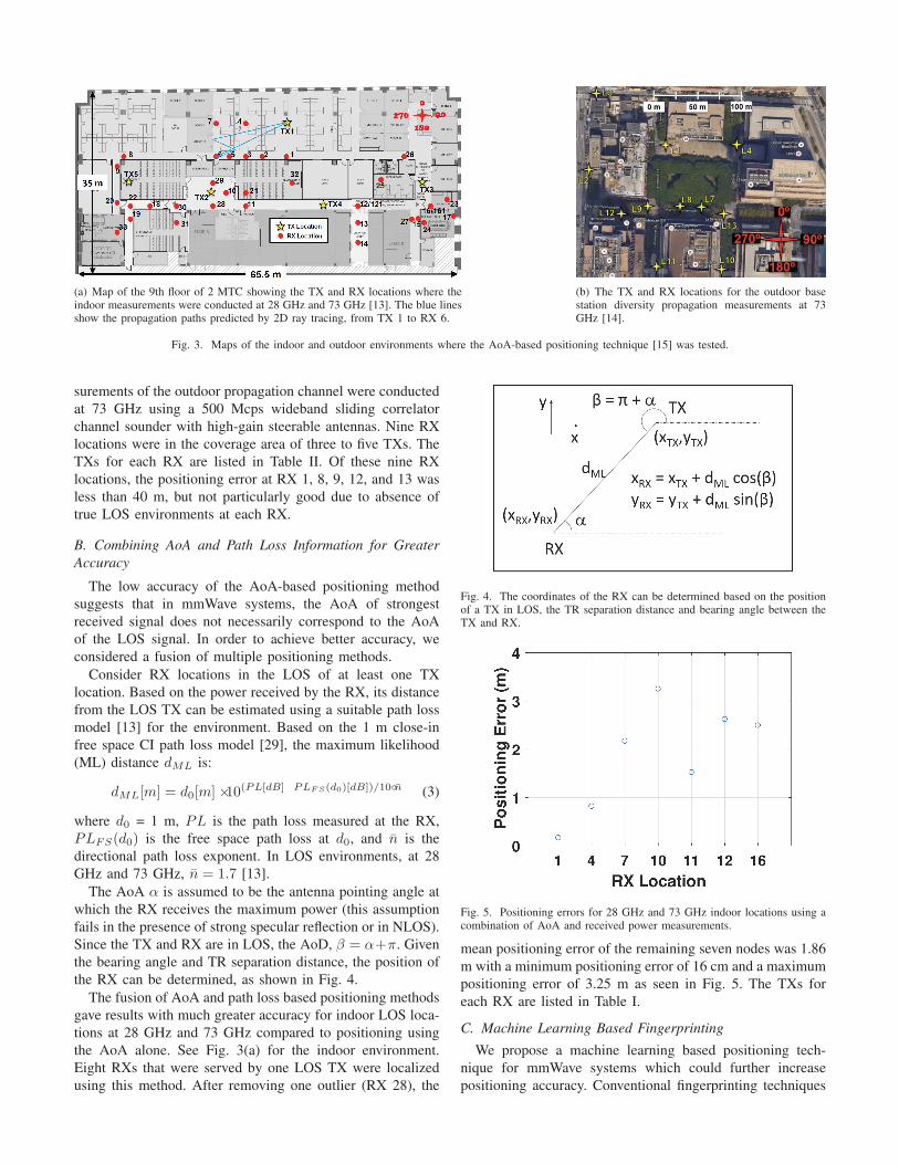
The AoA α is assumed to be the antenna pointing angle at
which the RX receives the maximum power (this assumption
fails in the presence of strong specular reflection or in NLOS).
Since the TX and RX are in LOS, the AoD, β = α+π. Given
the bearing angle and TR separation distance, the position of
the RX can be determined, as shown in Fig. 4.
The fusion of AoA and path loss based positioning methods
gave results with much greater accuracy for indoor LOS loca-
tions at 28 GHz and 73 GHz compared to positioning using
the AoA alone. See Fig. 3(a) for the indoor environment.
Eight RXs that were served by one LOS TX were localized
using this method. After removing one outlier (RX 28), the
Fig. 4. The coordinates of the RX can be determined based on the positionof a TX in LOS, the TR separation distance and bearing angle between theTX and RX.
Fig. 5. Positioning errors for 28 GHz and 73 GHz indoor locations using acombination of AoA and received power measurements.
mean positioning error of the remaining seven nodes was 1.86
m with a minimum positioning error of 16 cm and a maximum
positioning error of 3.25 m as seen in Fig. 5. The TXs for
each RX are listed in Table I.
C. Machine Learning Based Fingerprinting
We propose a machine learning based positioning tech-
nique for mmWave systems which could further increase
positioning accuracy. Conventional fingerprinting techniques
map the RSSI throughout the environment in consideration
[17]. We propose to also measure the AoA and ToA to
increase redundancy and improve resilience to changes in the
environment since such capabilities will naturally be available
in wideband, narrowbeam mmWave and THz systems.
RSSI, AoA, and ToA are measured over a grid of lo-
cations from multiple TXs. These measured parameters are
then stored in a database, off-line. Using these pre-measured
signals, the user’s position is estimated to be the most likely
location that best matches all measured parameter values. Ow-
ing to the fine resolution of ToA measurements possible due
to the wide bandwidth available, centimeter level positioning
accuracy could be achieved, and we are presently exploring
this approach.
V. LOCALIZATION BASED ON CONNECTIVITY AND RSSI
RANK
A grid-based localization algorithm for sensor networks
was proposed in [30]. Each user ranks all the anchor nodes
based on RSSI. Ideally, RSSI values decrease monotonically
with distance. Hence, by ordering the RSSI values, the user
can order the anchor nodes based on their distance. In a sensor
network with m anchor nodes, the ordering is stored in an m-
dimensional vector called the distance rank vector.
A. The Distance Rank Vector
The 2D plane can be subdivided into sub-regions based on
the ordering of distances of the user from anchor nodes. All
points within a sub-region have the same ordering and hence
have identical distance rank vectors. Thus, the user can be
localized to one of the many sub-regions in the plane based
on the user’s RSSI rank vector [30].
When there is an RSSI measurement error (or if RSSI does
not monotonically decrease with distance due to multipath
or obstructions/reflections), the RSSI vector may produce
an infeasible distance rank vector. In this case, the user is
localized to the sub-region whose distance rank vector is
closest to the measured distance rank vector. The closeness
of two distance rank vectors can be measured using the
Spearman rank order correlation coefficient, ρ [-1,1], with
close distance rank vectors having greater values of ρ [30].
B. Grid-based Localization
For m anchor nodes, each user has O(m5) worst-case
space and O(m5 log2 m) worst-case time complexity to create
the distance rank vector [30]. For resource-constrained user
nodes, real time computation may not be possible. In such
cases, a grid-based approach can be used.
A region called the estimation rectangle (ER) is defined,
surrounding each anchor node, based on an estimate of the
anchor node’s communication range. The ER is then divided
into square-shaped grids, based on a predefined grid size.
Within the area of intersection of ERs of all anchor nodes
belonging to the user’s distance rank vector, the set of grids
with maximal Spearman correlation coefficient is called the
residence area of the user. The user’s position is estimated to
be the centroid of all grids within the residence area [30].
C. Performance of the RSSI Rank-Based Algorithm UsingOutdoor Measurement Data
The RSSI rank-based algorithm was tested on the base-
station diversity data described in [14] which was obtained
using the system described in section IV-A. The maximum
range of communication was taken to be 200 m, the typical
cell radius of a small-cell mmWave deployment. The TXs for
each RX are listed in Table II. The average positioning error
was 34 m for grids with a grid length of 20 m. There was
no accuracy improvement when the grid length was further
reduced. Of the nine RX locations, L1, L2, L7, L9 and L10
had a positioning error less than 20 m.The mean distance error for the RSSI rank-based algorithm
is quite large when there are limited known nodes with large
coverage areas. However, the RSSI rank-based algorithm suc-
cessfully localized the user to the correct sub-region, which
could be used to determine the room or building location the
user is in by positioning the anchor nodes so that sub-regions
coincide with room or building boundaries.
VI. RAY TRACING OF MMWAVE COMMUNICATION
CHANNELS
Real-world mmWave measurements are time intensive and
expensive. In order to accurately predict received signal
characteristics such as received power, needed to investigate
position location algorithms, AoA and ToA, ray tracing may
be used, so long as the ray tracer is extremely accurate and
calibrated to observable measurements [31], [32]. To explore
likely position location accuracy, a 2-D ray tracer has been
developed for this paper.Ray tracing was done by brute force, by launching 100
rays uniformly over 360 in the azimuth plane at zero degree
elevation from TX locations previously measured in [13]. In
every direction, on encountering an intersection with an ob-
struction, simple reflected and transmitted ray directions were
calculated, based on Fresnel’s equations, with an effective
relative permittivity of εr = 5.0 [32]. New source rays at each
boundary were then recursively traced in the reflection and
transmission directions to the next encountered obstruction
on the propagating ray path. Path loss was calculated based
on the CI LOS path loss model [29], with a TR separation
distance equal to the total propagated ray length. Reflection
and transmission losses at each obstruction were computed
based on Fresnel’s equations [32]. Rays were considered
to contribute to the received power if they fell within the
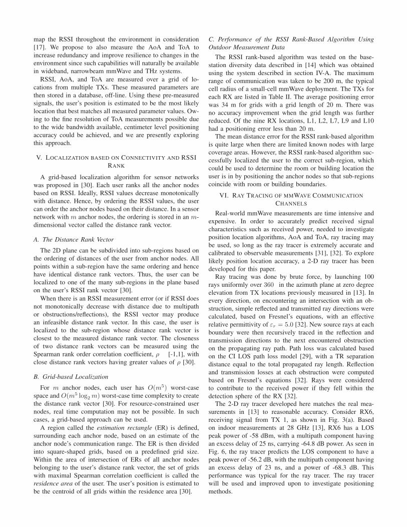
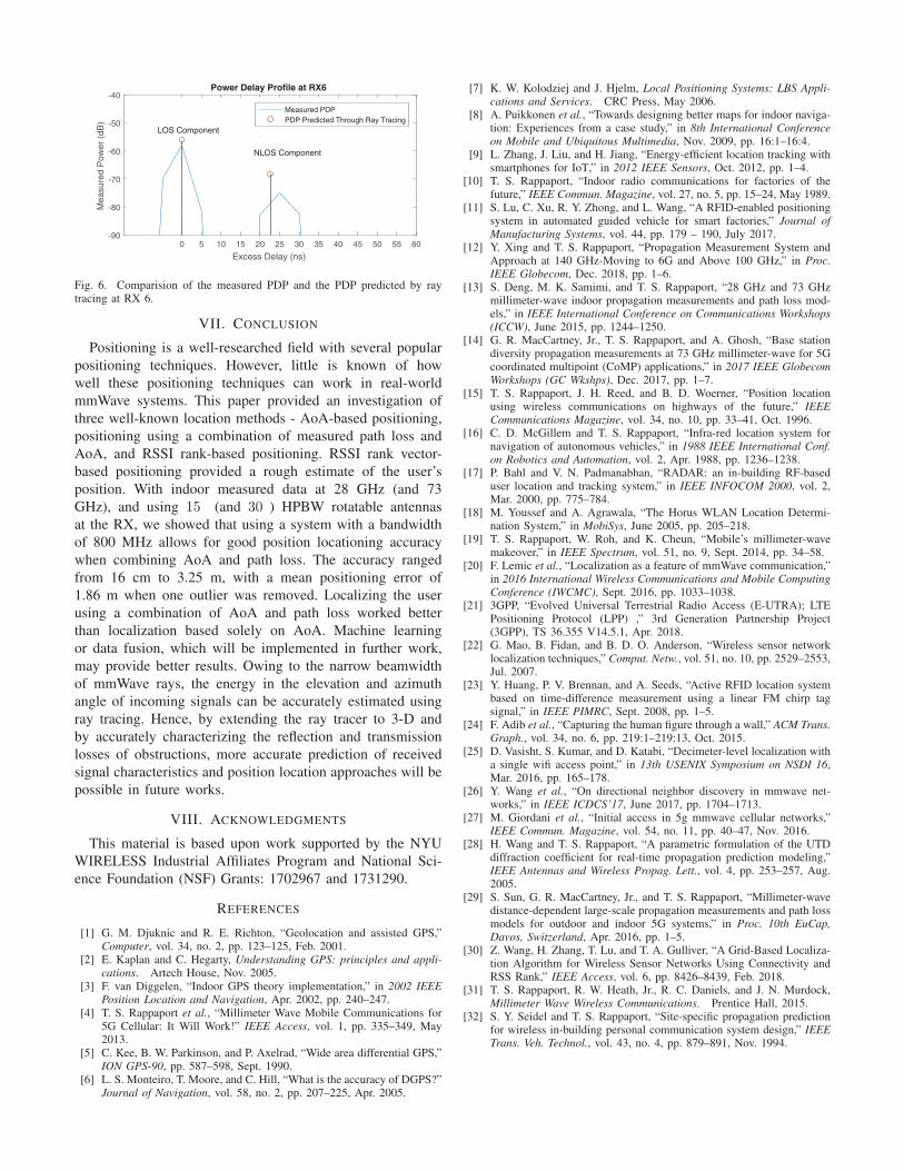
detection sphere of the RX [32].The 2-D ray tracer developed here matches the real mea-
surements in [13] to reasonable accuracy. Consider RX6,
receiving signal from TX 1, as shown in Fig. 3(a). Based
on indoor measurements at 28 GHz [13], RX6 has a LOS
peak power of -58 dBm, with a multipath component having
an excess delay of 25 ns, carrying -64.8 dB power. As seen in
Fig. 6, the ray tracer predicts the LOS component to have a
peak power of -56.2 dB, with the multipath component having
an excess delay of 23 ns, and a power of -68.3 dB. This
performance was typical for the ray tracer. The ray tracer
will be used and improved upon to investigate positioning
methods.
0 5 10 15 20 25 30 35 40 45 50 55 60
Excess Delay (ns)
-90
-80
-70
-60
-50
-40M
easu
red
Pow
er (
dB)
Power Delay Profile at RX6
Measured PDPPDP Predicted Through Ray Tracing
LOS Component
NLOS Component
Fig. 6. Comparision of the measured PDP and the PDP predicted by raytracing at RX 6.
VII. CONCLUSION
Positioning is a well-researched field with several popular
positioning techniques. However, little is known of how
well these positioning techniques can work in real-world
mmWave systems. This paper provided an investigation of
three well-known location methods - AoA-based positioning,
positioning using a combination of measured path loss and
AoA, and RSSI rank-based positioning. RSSI rank vector-
based positioning provided a rough estimate of the user’s
position. With indoor measured data at 28 GHz (and 73
GHz), and using 15 (and 30 ) HPBW rotatable antennas
at the RX, we showed that using a system with a bandwidth
of 800 MHz allows for good position locationing accuracy
when combining AoA and path loss. The accuracy ranged
from 16 cm to 3.25 m, with a mean positioning error of
1.86 m when one outlier was removed. Localizing the user
using a combination of AoA and path loss worked better
than localization based solely on AoA. Machine learning
or data fusion, which will be implemented in further work,
may provide better results. Owing to the narrow beamwidth
of mmWave rays, the energy in the elevation and azimuth
angle of incoming signals can be accurately estimated using
ray tracing. Hence, by extending the ray tracer to 3-D and
by accurately characterizing the reflection and transmission
losses of obstructions, more accurate prediction of received
signal characteristics and position location approaches will be
possible in future works.
VIII. ACKNOWLEDGMENTS
This material is based upon work supported by the NYU
WIRELESS Industrial Affiliates Program and National Sci-
ence Foundation (NSF) Grants: 1702967 and 1731290.
REFERENCES
[1] G. M. Djuknic and R. E. Richton, “Geolocation and assisted GPS,”Computer, vol. 34, no. 2, pp. 123–125, Feb. 2001.
[2] E. Kaplan and C. Hegarty, Understanding GPS: principles and appli-cations. Artech House, Nov. 2005.
[3] F. van Diggelen, “Indoor GPS theory implementation,” in 2002 IEEEPosition Location and Navigation, Apr. 2002, pp. 240–247.
[4] T. S. Rappaport et al., “Millimeter Wave Mobile Communications for5G Cellular: It Will Work!” IEEE Access, vol. 1, pp. 335–349, May2013.
[5] C. Kee, B. W. Parkinson, and P. Axelrad, “Wide area differential GPS,”ION GPS-90, pp. 587–598, Sept. 1990.
[6] L. S. Monteiro, T. Moore, and C. Hill, “What is the accuracy of DGPS?”Journal of Navigation, vol. 58, no. 2, pp. 207–225, Apr. 2005.
[7] K. W. Kolodziej and J. Hjelm, Local Positioning Systems: LBS Appli-cations and Services. CRC Press, May 2006.
[8] A. Puikkonen et al., “Towards designing better maps for indoor naviga-tion: Experiences from a case study,” in 8th International Conferenceon Mobile and Ubiquitous Multimedia, Nov. 2009, pp. 16:1–16:4.
[9] L. Zhang, J. Liu, and H. Jiang, “Energy-efficient location tracking withsmartphones for IoT,” in 2012 IEEE Sensors, Oct. 2012, pp. 1–4.
[10] T. S. Rappaport, “Indoor radio communications for factories of thefuture,” IEEE Commun. Magazine, vol. 27, no. 5, pp. 15–24, May 1989.
[11] S. Lu, C. Xu, R. Y. Zhong, and L. Wang, “A RFID-enabled positioningsystem in automated guided vehicle for smart factories,” Journal ofManufacturing Systems, vol. 44, pp. 179 – 190, July 2017.
[12] Y. Xing and T. S. Rappaport, “Propagation Measurement System andApproach at 140 GHz-Moving to 6G and Above 100 GHz,” in Proc.IEEE Globecom, Dec. 2018, pp. 1–6.
[13] S. Deng, M. K. Samimi, and T. S. Rappaport, “28 GHz and 73 GHzmillimeter-wave indoor propagation measurements and path loss mod-els,” in IEEE International Conference on Communications Workshops(ICCW), June 2015, pp. 1244–1250.
[14] G. R. MacCartney, Jr., T. S. Rappaport, and A. Ghosh, “Base stationdiversity propagation measurements at 73 GHz millimeter-wave for 5Gcoordinated multipoint (CoMP) applications,” in 2017 IEEE GlobecomWorkshops (GC Wkshps), Dec. 2017, pp. 1–7.
[15] T. S. Rappaport, J. H. Reed, and B. D. Woerner, “Position locationusing wireless communications on highways of the future,” IEEECommunications Magazine, vol. 34, no. 10, pp. 33–41, Oct. 1996.
[16] C. D. McGillem and T. S. Rappaport, “Infra-red location system fornavigation of autonomous vehicles,” in 1988 IEEE International Conf.on Robotics and Automation, vol. 2, Apr. 1988, pp. 1236–1238.
[17] P. Bahl and V. N. Padmanabhan, “RADAR: an in-building RF-baseduser location and tracking system,” in IEEE INFOCOM 2000, vol. 2,Mar. 2000, pp. 775–784.
[18] M. Youssef and A. Agrawala, “The Horus WLAN Location Determi-nation System,” in MobiSys, June 2005, pp. 205–218.
[19] T. S. Rappaport, W. Roh, and K. Cheun, “Mobile’s millimeter-wavemakeover,” in IEEE Spectrum, vol. 51, no. 9, Sept. 2014, pp. 34–58.
[20] F. Lemic et al., “Localization as a feature of mmWave communication,”in 2016 International Wireless Communications and Mobile ComputingConference (IWCMC), Sept. 2016, pp. 1033–1038.
[21] 3GPP, “Evolved Universal Terrestrial Radio Access (E-UTRA); LTEPositioning Protocol (LPP) ,” 3rd Generation Partnership Project(3GPP), TS 36.355 V14.5.1, Apr. 2018.
[22] G. Mao, B. Fidan, and B. D. O. Anderson, “Wireless sensor networklocalization techniques,” Comput. Netw., vol. 51, no. 10, pp. 2529–2553,Jul. 2007.
[23] Y. Huang, P. V. Brennan, and A. Seeds, “Active RFID location systembased on time-difference measurement using a linear FM chirp tagsignal,” in IEEE PIMRC, Sept. 2008, pp. 1–5.
[24] F. Adib et al., “Capturing the human figure through a wall,” ACM Trans.Graph., vol. 34, no. 6, pp. 219:1–219:13, Oct. 2015.
[25] D. Vasisht, S. Kumar, and D. Katabi, “Decimeter-level localization witha single wifi access point,” in 13th USENIX Symposium on NSDI 16,Mar. 2016, pp. 165–178.
[26] Y. Wang et al., “On directional neighbor discovery in mmwave net-works,” in IEEE ICDCS’17, June 2017, pp. 1704–1713.
[27] M. Giordani et al., “Initial access in 5g mmwave cellular networks,”IEEE Commun. Magazine, vol. 54, no. 11, pp. 40–47, Nov. 2016.
[28] H. Wang and T. S. Rappaport, “A parametric formulation of the UTDdiffraction coefficient for real-time propagation prediction modeling,”IEEE Antennas and Wireless Propag. Lett., vol. 4, pp. 253–257, Aug.2005.
[29] S. Sun, G. R. MacCartney, Jr., and T. S. Rappaport, “Millimeter-wavedistance-dependent large-scale propagation measurements and path lossmodels for outdoor and indoor 5G systems,” in Proc. 10th EuCap,Davos, Switzerland, Apr. 2016, pp. 1–5.
[30] Z. Wang, H. Zhang, T. Lu, and T. A. Gulliver, “A Grid-Based Localiza-tion Algorithm for Wireless Sensor Networks Using Connectivity andRSS Rank,” IEEE Access, vol. 6, pp. 8426–8439, Feb. 2018.
[31] T. S. Rappaport, R. W. Heath, Jr., R. C. Daniels, and J. N. Murdock,Millimeter Wave Wireless Communications. Prentice Hall, 2015.
[32] S. Y. Seidel and T. S. Rappaport, “Site-specific propagation predictionfor wireless in-building personal communication system design,” IEEETrans. Veh. Technol., vol. 43, no. 4, pp. 879–891, Nov. 1994.