portfolios in the ibex 35 before and after the global
TRANSCRIPT
Portfolios in the Ibex 35 before and after the Global Financial Crisis
Víctor M. Adame a, Fernando Fernández-Rodríguezb and Simon Sosvilla-Rivero c
aUniversidad Complutense de Madrid, Madrid, Spain; bUniversidad de Las Palmas de Gran Canaria, Las Palmas de Gran Canaria, Spain;cComplutense Institute for International Studies, Universidad Complutense de Madrid, Madrid, Spain
ABSTRACT
In this article, we present an analysis of the effectiveness of various portfolio optimizationstrategies applied to the stocks included in the Spanish Ibex 35 index, for a period of 14 years,from 2001 until 2014. The period under study includes episodes of volatility and instability infinancial markets, incorporating the Global Financial Crisis and the European Sovereign DebtCrisis. This implies a challenge in portfolio optimization strategies since the methodologies arerestricted to the assignment of positive weights. We have taken for asset allocation the dailyreturns with an estimation window equal to 1 year and we hold portfolio assets for another year.This article attempts to influence the discussion over whether the naive diversification proves tobe an effective strategy as opposed to portfolio optimization models. For that, we evaluate theout-of-sample performance of 15 strategies for asset allocation in the Ibex 35, before and after ofthe Global Financial Crisis. Our results suggest that a large number of strategies outperform tothe 1/N rule and to the Ibex 35 index in terms of return, Sharpe ratio and lower VaR and CVaR.The mean-variance portfolio of Markowitz with short-sale constraints is the only strategy thatrenders a Sharpe ratio statistically different from Ibex 35 index in the 2001–2007 and 2008–2014time periods.
KEYWORDS
Finance: portfolio choice;investment decisions;econometrics;minimum-varianceportfolios; robust statistics;out-of-sample performance
JEL CLASSIFICATION
C61; G11; C14
I. Introduction
Markowitz (1952, 1959) suggested that a rationalinvestor should choose a portfolio with the lowestrisk for a given level of return instead of investing inindividual assets, calling these portfolios as efficient.This approach has been the first model of portfolioselection in the literature, which is known as mean-variance of Markowitz. Although the mean-variancemethodology has become the central base of the clas-sical finance, leading directly to the development of theCapital Asset Pricing Model (CAPM) by Sharpe(1964), Lintner (1965) andMossin (1966), the practicalapplication is surrounded by difficulties due to theirpoor out-of-sample performance since the expectedreturns are estimated based only on sample informa-tion, which results in an estimation error.
A latter approach to addressing the estimationerror involves the application of Bayesian techni-ques, or shrinkage estimators. Jorion (1991) use theBayesian approach to overcome the weakness of theexpected returns estimate only by sample
information. More recent approaches are based onthe asset pricing model (see Pástor 2000; Pástor andStambaugh 2000); and the imposition of rules forshort-selling constraint (e.g., Frost and Savarino1988; Chopra 1993; Jagannathan and Ma 2003).Similarly, in the literature have been introduced theminimum-variance portfolios, based on the estima-tion of the covariance matrix, which is not generallyas sensitive to estimation error and provides a betterout-of-sample performance (see Chan, Karceski, andLakonishok 1999; Jagannathan and Ma 2003; amongothers).
It is also common to use robust optimizationtechniques to overcome the problems of stochasticprogramming techniques (see, for example,Quaranta and Zaffaroni 2008; DeMiguel, Garlappi,and Uppal 2009; DeMiguel and Nogales 2009; Harrisand Mazibas 2013; Allen et al. 2014a, 2014b; Xing,Hu, and Yang 2014.). Choueifaty and Coignard(2008) and Choueifaty, Froidure, and Reynier(2013) proposed an approach based on the portfoliowith the highest ratio of diversification. In addition,
Supplemental data for this article can be accessed here.
CONTACT Simon Sosvilla-Rivero [email protected] Complutense Institute for International Studies, Universidad Complutense de Madrid, Campusde Somosaguas, 28223 Madrid, Spain
APPLIED ECONOMICS, 2016
VOL. 48, NO. 40, 3826–3847
http://dx.doi.org/10.1080/00036846.2016.1145352
© 2016 Taylor & Francis
Qian (2005, 2006, 2011) introduced the portfoliowith equal contribution to risk, which assigns differ-ent weights to assets so that their contribution to theoverall volatility of the portfolio is proportional; theproperties of this strategy were analysed by Maillard,Roncalli, and Teïletche (2010). These methodologies
aim to defend against the possible uncertainty in the
parameters of the problem given that these are not
exactly known.
In recent years, the interest of the authorities has
increased considerably in the measurement of the
effects of unexpected losses associated with extreme
events in financial markets. This leads directly to
improved methodologies for measurement and
quantification of risk. In this sense, it is considered
that the traditional framework of mean-variance,
frequently used in the selection of efficient portfo-
lios, should be revised to introduce more complex
risk measures than the simple SD (that is, risk mea-
sures based on the quantile). This is the context that
explains the choice of Value at Risk (VaR) as syn-
thetic risk measure that can express the market risk
of a financial asset or portfolio (JP Morgan 1994).
Nevertheless, VaR has been the subject of strong
criticism, despite the widespread use in banking
supervision, VaR lacks subadditivity so it is not a
coherent risk measure for the general distribution of
loss, and this goes against the diversification princi-
ple (see Artzner et al. 1997, 1999).
Moreover, the absence of convexity of VaR causes
considerable difficulties in portfolio selection models
based on minimizing the same. Furthermore, the
VaR has been criticized for not being able to quan-
tify the so-called ‘tail risk’. This has led some
researchers to define new risk measures such as
Conditional Value at Risk (ES or CVaR) (see
Rockafellar and Uryasev 2000, 2002; Pflug 2000;
Gaivoronski and Pflug 2005).
There has been a rapid impulse in recent years in
the literature about the use of CVaR in portfolio
theory. Additionally, the CVaR has the mathematical
advantage that can be minimized using linear pro-
gramming methods. A simple description of the
approach to minimize CVaR and CVaR constrained
optimization problems can be found in Chekhlov,
Uryasev, and Zabarankin (2000). Krokhmal,
Palmquist, and Uryasev (2002) compared the CVaR
and Conditional Drawdown-at-Risk (CDAR)
approaches to minimal risk portfolios in some
hedge funds. Agarwal and Naik (2004), and
Giamouridis and Vrontos (2007) compared the tra-
ditional mean-variance approach with CVaR portfo-
lios built using strategies of hedge funds.
Our objective in this article is to compare the out-
of-sample performance of the naive strategy regard-
ing various models for the construction of efficient
portfolios. It should be noted that a debate exists in
the literature about whether the gains from optimi-
zation are reduced by estimation errors or uncer-
tainty in the parameters, which influence in the
portfolio optimization process. In this sense, there
is no consensus in the literature on whether the
naive diversification is more effective than other
portfolio strategies (see recent works, such as
DeMiguel, Garlappi, and Uppal 2009; Tu and Zhou
2011; Kirby and Ostdiek 2012; and Allen et al. 2014a,
2014b).
For this purpose, we considered a number of
optimization models: (a) the classical mean-variance
approach (Markowitz 1952, 1959) and the minimum
variance approach (Jagannathan and Ma 2003); (b)
robust optimization techniques, as the most diversi-
fied portfolio(see Choueifaty and Coignard 2008;
Choueifaty, Froidure, and Reynier 2013) and the
equally weighted risk contributions portfolios (see
Qian 2005, 2006, 2011); (c) portfolio optimization
based on Conditional Value at Risk, ‘CVaR’
(Rockafellar and Uryasev 2000, 2002; Alexander
and Baptista 2004; Quaranta and Zaffaroni 2008);
(d) functional approach based on risk measures
such as the ‘Maximum draw-down’ (MaxDD), the
‘Average draw-down’ (AvDD), and the ‘Conditional
draw-down at risk’ (CDAR), all proposed by
Chekhlov, Uryasev, and Zabarankin (2000, 2005);
as well as the Conditional draw-down at risk,
‘MinCDaR’ (see Chekhlov, Uryasev, and
Zabarankin 2005; Kuutan 2007); (e) Young (1998)’s
minimax optimization model, based on minimizing
risk and optimizing the risk/return ratio; (f) applica-
tion of Copulae theory to build the minimum tail-
dependent portfolio, where the variance–covariance
matrix is replaced by lower tail dependence coeffi-
cient (see Frahm, Junker, and Schmidt 2005; Fischer
and Dörflinger 2006; Schmidt and Stadtmüller
2006); and (g) a defensive approach to systemic
risk by beta strategy (‘Low Beta’). The beta coeffi-
cient (β) is used to assess systemic risk of an asset in
the CAPM model (see Sharpe 1964; Lintner 1965;
APPLIED ECONOMICS 3827
Mossin 1966), as related volatility of an asset, mar-ket, and the correlation between them. To conclude,we impose a short-selling constraint in the models.
Following DeMiguel, Garlappi, and Uppal (2009),it is of paramount importance to compare the resultsof different methodologies with the ‘naive diversifi-cation of 1/N’, which assigns equal weight to therisky assets. The 1/N strategy has proved as a diffi-cult alternative to beat, demonstrating the practicaldifficulties to obtain an efficient portfolio(DeMiguel, Garlappi, and Uppal 2009; Allen et al.2014a.). Therefore, we propose an efficiency analysisof the various methodologies compared with thenaive diversification of 1/N and the main Spanishstock index, Ibex 35.
For the evaluation of the out-of-sample perfor-mance, we use five criteria. The first one is theSharpe ratio as a measure of the excess return(Sharpe 1994). To test if the Sharpe ratio of twostrategies is statistically different, we obtain thep-value of the difference, using the approach suggestedby Jobson and Korkie (1981), after making the correc-tion pointed out in Memmel (2003). Similarly, wecalculate the diversification ratio as a measure of thedegree of portfolio diversification (Choueifaty andCoignard 2008; Choueifaty, Froidure, and Reynier2013.); the concentration ratio, which is simply thenormalized Herfindahl–Hirschmann index (seeHirschman 1964); The Value at Risk (VaR) as syn-thetic risk measure that can express the market risk ofa financial asset or portfolio, and the expected shortfall(ES or CVaR) as a coherent risk measure that takesinto account the ‘tail risk’.
As for the data, we use a sample of the daily valuesof the stocks included into the Ibex 35 index. TheIbex 35 index is the official index of the SpanishContinuous Market. The index is comprised of the35 most liquid stocks traded on the Continuous mar-ket. The prices are adjusted for dividend and these aretaken from Datastream. The sample period, runningfrom 1 January 2000 to 31 December 2014, encom-passes two episodes of turmoil in financial markets:the Global Financial Crisis, which began in 2008; andthe European Sovereign Debt Crisis. The data set isavailable at the link provided in the supplementarydata set section of this paper.
The Spanish stock market has combined from theearlier nineties, when its main stock index Ibex 35was created; sharp rises with periods of losses.Additionally, the improvement on the technical,operational and organizational systems supportingthe market has enabled it to channel large volumesof investment and have made it more transparent,liquid and effective. The pooling of interests hasenabled Spain to reach a significant size in theEuropean context and a diversified structure thatcovers the whole chain of activities in the markets,from trading to settlement. The Ibex 35 stock indexhas been the subject of numerous studies. For exam-ple, Matallin and Nieto (2002) analyse the manage-ment of risky assets and mixed risky mutual funds inrelation to alternative investment in the Ibex 35.Matallín and Fernández-Izquierdo (2003) examine
the extent of the passive timing effect in portfolio
management using different portfolios representa-
tive of different levels of risk for the Spanish market.
Rosillo, De La Fuente, and Brugos (2013) examine
the result of the application of technical analysis in
the Spanish stock market using different indicators
of the quantitative analysis. Fernandez-Perez,
Fernández-Rodríguez, and Sosvilla-Rivero (2014)
show that the term structure of interest rates has
some information content that helps to better fore-
cast the probability of bear markets in the Ibex 35.
Finally, Miralles-Quirós, Miralles-Quirós, and Daza-
Izquierdo (2015) propose different trading strategies
for the Ibex 35, based on the combination of differ-
ent strategies and on the predictive power of the
returns from the opening of the Spanish stock mar-
ket and the US market.
We used the daily returns with an estimate win-
dow equal to one year, 252 days. Therefore, the
portfolios have been built for a sample size
Nt ¼ 252, and the results have been evaluated out
of sample for the next period Ntþ1, (see Table 1). We
considered only those stocks that have shown con-
tinuity within the index during the period of
estimation.1 We show, in Table 1, the assets number
in each period. In the Appendix (Table A2), we
report the asset ´considered in each time period.
The rest of the article is organized as follows. In
Section 2, we describe the various methodologies
1In the Appendix of this article, we include a summary table with the main statistical of the portfolios, and another table with the assets that we consider ineach period.
3828 V. M. ADAME ET AL.
used for portfolio construction. In Section 3, we
explain the methodology for performance evalua-
tion. In Section 4, we show the results against the
Ibex 35 index and the naive strategy of 1/N. In
Section 5, we present some concluding remarks.
II. Methodological description
Mean-variance portfolio
The efficient frontier of mean-variance is defined as
the set of values μi; σi2
!
that resolves the following
multi-objective optimization problem:
maxwμ; (1)
minw
Xw;
s:t:w1 ¼ 1;
where w is the N ! 1ð Þ vector of weights and Σ
denotes the variance–covariance matrix of asset
returns with elements outside the diagonal and σij
σ2i the ith element of the main diagonal.
Each point on the efficient frontier μi; σ2i
!
corre-
sponds to an efficient portfolio where the investor
gets a maximum return for a given level of risk σi.
The efficient frontier of mean-variance reflects the
relationship between return and risk, introducing
the trade-off concept of risk–return in the financial
markets. Therefore, it describe the level of return μi
given a risk exposure σi, or seen from a reverse
perspective, the lower variability σi for a return
level μi (Markowitz 1952, 1959).
A risk-averse rational investor will make an
investment decision on the efficient frontier when
the risky asset returns exhibit a multivariate normal
distribution or if her utility function is quadratic.
The best choice will reflect the investor’s willingness
to trade off risk against expected return.
To solve efficiently the problem of quadratic opti-
mization with two objectives described above, the
problem can be converted into a quadratic optimiza-
tion problem for different levels of return μi (Tsao
2010).
minw
Xw; (2)
s:t: wμ ¼ μi;
s:t: w1 ¼ 1;
s:t: w $ 0:
The expected return and the variance of the port-
folio are wμ, and w
P
w; respectively. In this article,
we solve the above quadratic optimization problem
and establish an expected return μi equal to the
average return on the assets that are considered in
the optimization problem. We have also included a
short-selling restriction such that w $ 0.
Minimum-variance portfolio
We use the previous optimization problem to assign
the weights w to each asset in the minimum-variance
portfolio, but not including the restriction on
returns, wμ ¼ μi.
minw
X
w; (3)
s:t: w1 ¼ 1;
s:t: w $ 0:
We obtain the portfolio that provides the minimum
variance σ2i , given any return μi in the efficient frontier
of mean-variance. In contrast to the mean-variance
portfolio, the minimum variance weight vector does
not depend of the expected return on assets (see
Jagannathan and Ma 2003, for a study of the properties).
Naive diversification
Several studies confirm the existence of some inves-
tors who distribute their wealth through naive diver-
sification strategy. Typically they invest in a few
assets alike (see Benartzi and Thaler 2001;
Huberman and Jiang 2006). This fact does not
prove that the naive diversification is a good strat-
egy, since investors may select a portfolio that is not
within the efficient frontier, or she may choose the
wrong point in it. Both situations involve a cost,
Table 1. Number of assets by time period.
Time period Number of risky assets
03/01/2000–28/12/2001 2102/01/2001–30/12/2002 2302/01/2002–30/12/2003 2502/01/2003–30/12/2004 2602/01/2004–30/12/2005 2903/01/2005–29/12/2006 2902/01/2006–28/12/2007 3002/01/2007–30/12/2008 2902/01/2008–30/12/2009 3002/01/2009–30/12/2010 3104/01/2010–30/12/2011 3103/01/2011–31/12/2012 3202/01/2012–31/12/2013 3302/01/2013–31/12/2014 35
APPLIED ECONOMICS 3829
where the second cost is the most important (see
Brennan and Torous 1999).
The naive strategy involves a weight distribution
wj ¼ 1=N for all risky assets in the portfolio. This
strategy ignores the data and does not involve any
estimation or optimization. DeMiguel, Garlappi, and
Uppal (2009) suggest that the expected returns are
proportional to total risk instead systematic risk.
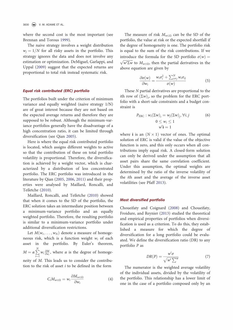
Equal risk contributed (ERC) portfolio
The portfolios built under the criterion of minimum
variance and equally weighted (naive strategy 1/N)
are of great interest because they are not based on
the expected average returns and therefore they are
supposed to be robust. Although the minimum-var-
iance portfolios generally have the disadvantage of a
high concentration ratio, it can be limited through
diversification (see Qian 2005).
Here is where the equal risk contributed portfolio
is located, which assigns different weights to active
so that the contribution of these on total portfolio
volatility is proportional. Therefore, the diversifica-
tion is achieved by a weight vector, which is char-
acterized by a distribution of less concentrated
portfolio. The ERC portfolio was introduced in the
literature by Qian (2005, 2006, 2011) and their prop-
erties were analysed by Maillard, Roncalli, and
Teïletche (2010).
Maillard, Roncalli, and Teïletche (2010) showed
that when it comes to the SD of the portfolio, the
ERC solution takes an intermediate position between
a minimum-variance portfolio and an equally
weighted portfolio. Therefore, the resulting portfolio
is similar to a minimum-variance portfolio under
additional diversification restrictions.
Let M wi; . . . ;wNð Þ denote a measure of homoge-
neous risk, which is a function weight wi of each
asset in the portfolio. By Euler’s theorem,
M ¼ α
P
N
i¼1
wi@M@wi
, where α is the degree of homoge-
neity of M. This leads us to consider the contribu-
tion to the risk of asset i to be defined in the form
CiMw2Ω ¼ wi@Mw2Ω@wi
(4)
The measure of risk Mw2Ω can be the SD of the
portfolio, the value at risk or the expected shortfall if
the degree of homogeneity is one. The portfolio risk
is equal to the sum of the risk contributions. If we
introduce the formula for the SD portfolio σ wð Þ ¼ffiffiffiffiffiffiffiffiffiffiffi
w0Σwp
to Mw2Ω, then the partial derivatives in the
above equation are given by
@σ wð Þ@wi
¼wiσ
2i þPN
i�j wiσij
σ wð Þ (5)
These N partial derivatives are proportional to the
ith row of Σwð Þi, so the problem for the ERC port-
folio with a short-sale constraints and a budget con-
straint is
PERC : wi Σwð Þi ¼ wj Σwð Þj;"i; j (6)
0 ' wi ' 1
w0i ¼ 1
where i is an N ( 1ð Þ vector of ones. The optimal
solution of ERC is valid if the value of the objective
function is zero, and this only occurs when all con-
tributions imply equal risk. A closed-form solution
can only be derived under the assumption that all
asset pairs share the same correlation coefficient.
Under this assumption, the optimal weights are
determined by the ratio of the inverse volatility of
the ith asset and the average of the inverse asset
volatilities (see Pfaff 2013).
Most diversified portfolio
Choueifaty and Coignard (2008) and Choueifaty,
Froidure, and Reynier (2013) studied the theoretical
and empirical properties of portfolios when diversi-
fication is used as a criterion. To do this, they estab-
lished a measure for which the degree of
diversification for a long portfolio could be evalu-
ated. We define the diversification ratio (DR) to any
portfolio P as
DR Pð Þ ¼ w0σffiffiffiffiffiffiffiffiffiffiffiffiffi
w0 Pwp (7)
The numerator is the weighted average volatility
of the individual assets, divided by the volatility of
the portfolio. This relationship has a lower limit of
one in the case of a portfolio composed only by an
3830 V. M. ADAME ET AL.

asset. Choueifaty, Froidure, and Reynier (2013) show
that the portfolio characterized by a highly concen-
trated or with strongly correlated asset returns
would qualify as being poorly diversified, so that
DR Pð Þ ¼ 1ffiffiffiffiffiffiffiffiffiffiffiffiffiffiffiffiffiffiffiffiffiffiffiffiffiffiffiffiffiffiffiffi
ρþ CRð Þ $ ρCRp (8)
where ρ denotes the volatility-weighted average cor-
relation and CR is the volatility-weighted concentra-
tion ratio. The DR only depends on the volatility-
weighted average correlations in the case of a naive
allocation.
Choueifaty, Froidure, and Reynier (2013) estab-
lished the conditions for the most diversified portfo-
lio by introducing a set of synthetic assets that share
the same volatility, such that
D Sð Þ ¼ S0PS
ffiffiffiffiffiffiffiffiffiffiffi
S0VsSp (9)
where S is a portfolio composed by synthetic assets,
and VS is the covariance matrix of synthetic assets. If
we have to S0PS ¼ 1, then to maximize D Sð Þ is
equivalent to maximizing 1ffiffiffiffiffiffiffiffi
S0VsSp under ΓS restric-
tions. VS is equal to the correlation matrix C of
initial assets, so that to maximize the diversification
ratio is equivalent to minimizing
S0CS: (10)
Thus, if the assets have the same volatility, the
diversification ratio is maximized by minimizing
w0Cw. Therefore, the objective function coincides
with the minimum-variance portfolio, although it is
used in the correlation matrix.
The impact of asset volatility is lower in the more
diversified portfolio compared with the minimum-
variance portfolio (see Pfaff 2013). The weights are
retrieved by intermediate vector rescaling weights
with SDs of asset returns. The optimal weight vector
is determined in two steps: first, an allocation is
determined that yields a solution for a least correlated
asset mix. This solution is then inversely adjusted by
the asset volatilities, and later, the weights of the
assets are adjusted inversely by their volatilities.
Minimum tail-dependent portfolio
Minimum tail-dependent portfolio is determined
through replacing the variance–covariance matrix
by matrix coefficients of lower tail dependence. In
that sense, the lower tail of the correlation coefficient
measures the dependence of the relationship
between the asset returns when these are extremely
negative. It is possible to find a scheme with various
nonparametric estimators for minimum tail-depen-
dent portfolio in Frahm, Junker, and Schmidt
(2005), and Fischer and Dörflinger (2006) and
Schmidt and Stadtmüller (2006).
The copulae theory was introduced by Sklar
(1959). Sklar’s theorem states that there is a C func-
tion, called copulae, which establishes the functional
relationship between the joint distribution and their
univariate marginal distribution functions. Formally,
let x ¼ x1; x2ð Þ be a two-dimensional random vector
with joint distribution function F x1; x2ð Þ and mar-
ginal distributions Fi xið Þ; i ¼ 1; 2; there will be a
copulae C u1; u2ð Þ such that
F x1; x2ð Þ ¼ P X1< x1;X2<x2ð Þ ¼ C F1 x1ð Þ; F2 x2ð Þð Þ:(11)
Moreover, Sklar’s theorem also provides that if Fi
are continuous, then the copulae C u1; u2ð Þ is unique.An important feature of copulae is that it allows dif-
ferent degrees of dependency on the tail. The upper
tail dependence λUð Þ exists when there is a positive
likelihood that positive outliers are given jointly; while
the lower tail dependence λL, exists when there is a
negative likelihood that negative outliers are given
jointly (see Boubaker and Sghaier 2013). Thereby, we
define the lower tail dependence coefficient as follows:
λL ¼ limu!0
C u; uð Þu
(12)
This limit can be interpreted as a conditional
probability, therefore, the lower tail dependence
coefficient is limited in the range 0; 1½ ): The limits
are: for an independent copulae λL ¼ 0ð Þ, and for a
co-monotonic copulae λL ¼ 1ð Þ. Nonparametric
estimators for λL are derived from empirical copulae.
For a given sample paired observations N,
X1;Y1ð Þ; . . . ; ðXN;YN), with order statistics X 1ð Þ *X 2ð Þ . . . * X Nð Þ and Y 1ð Þ * Y 2ð Þ . . . * Y Nð Þ, the
empirical copulae is defined as
CNi
N;j
N
# $
¼ 1
N
X
N
l¼1
I Xl * X ið Þ ^ Yl * Yj
& '
;
(13)
APPLIED ECONOMICS 3831
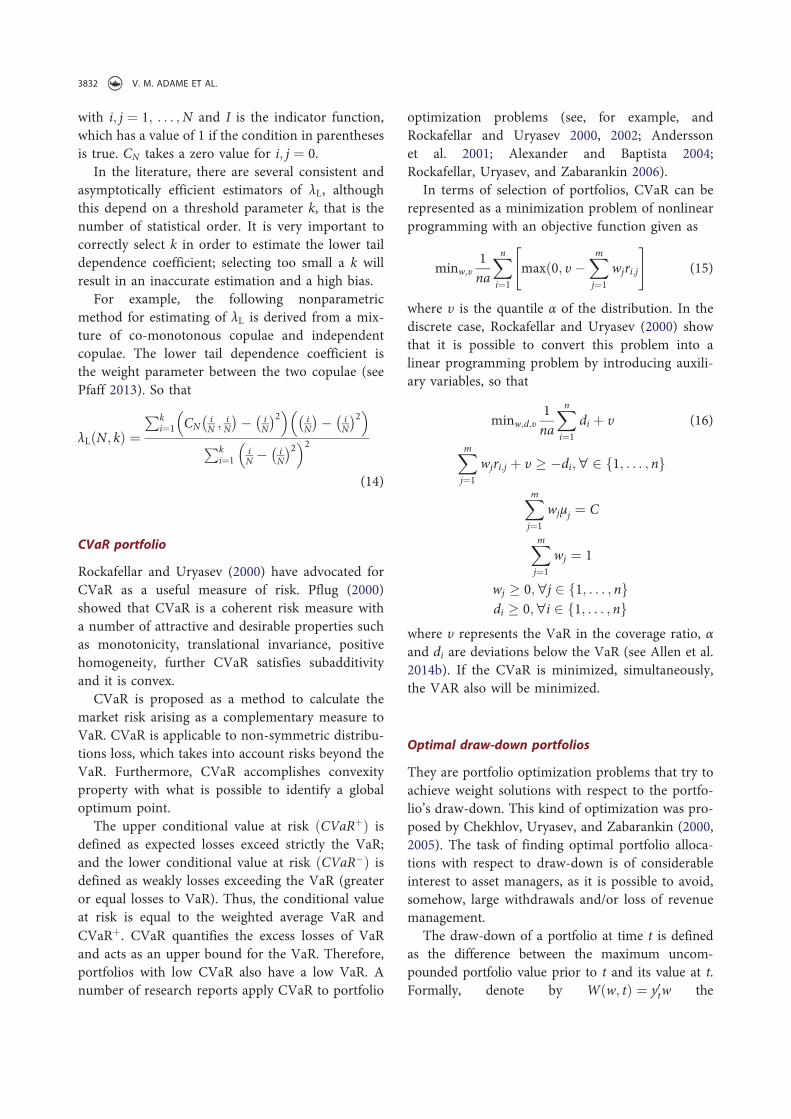
with i; j ¼ 1; . . . ;N and I is the indicator function,
which has a value of 1 if the condition in parentheses
is true. CN takes a zero value for i; j ¼ 0.
In the literature, there are several consistent and
asymptotically efficient estimators of λL, although
this depend on a threshold parameter k, that is the
number of statistical order. It is very important to
correctly select k in order to estimate the lower tail
dependence coefficient; selecting too small a k will
result in an inaccurate estimation and a high bias.
For example, the following nonparametric
method for estimating of λL is derived from a mix-
ture of co-monotonous copulae and independent
copulae. The lower tail dependence coefficient is
the weight parameter between the two copulae (see
Pfaff 2013). So that
λL N; kð Þ ¼Pk
i¼1 CNiN; iN
! "
# iN
! "2# $
iN
! "
# iN
! "2# $
Pki¼1
iN# i
N
! "2# $2
(14)
CVaR portfolio
Rockafellar and Uryasev (2000) have advocated for
CVaR as a useful measure of risk. Pflug (2000)
showed that CVaR is a coherent risk measure with
a number of attractive and desirable properties such
as monotonicity, translational invariance, positive
homogeneity, further CVaR satisfies subadditivity
and it is convex.
CVaR is proposed as a method to calculate the
market risk arising as a complementary measure to
VaR. CVaR is applicable to non-symmetric distribu-
tions loss, which takes into account risks beyond the
VaR. Furthermore, CVaR accomplishes convexity
property with what is possible to identify a global
optimum point.
The upper conditional value at risk CVaRþð Þ is
defined as expected losses exceed strictly the VaR;
and the lower conditional value at risk CVaR#ð Þ is
defined as weakly losses exceeding the VaR (greater
or equal losses to VaR). Thus, the conditional value
at risk is equal to the weighted average VaR and
CVaRþ. CVaR quantifies the excess losses of VaR
and acts as an upper bound for the VaR. Therefore,
portfolios with low CVaR also have a low VaR. A
number of research reports apply CVaR to portfolio
optimization problems (see, for example, and
Rockafellar and Uryasev 2000, 2002; Andersson
et al. 2001; Alexander and Baptista 2004;
Rockafellar, Uryasev, and Zabarankin 2006).
In terms of selection of portfolios, CVaR can be
represented as a minimization problem of nonlinear
programming with an objective function given as
minw;υ1
na
X
n
i¼1
maxð0; υ#X
m
j¼1
wjri;j
" #
(15)
where υ is the quantile α of the distribution. In the
discrete case, Rockafellar and Uryasev (2000) show
that it is possible to convert this problem into a
linear programming problem by introducing auxili-
ary variables, so that
minw;d;υ1
na
X
n
i¼1
di þ υ (16)
X
m
j¼1
wjri;j þ υ % #di;" 2 1; . . . ; nf g
X
m
j¼1
wjμj ¼ C
X
m
j¼1
wj ¼ 1
wj % 0;"j 2 1; . . . ; nf g
di % 0;"i 2 1; . . . ; nf g
where υ represents the VaR in the coverage ratio, α
and di are deviations below the VaR (see Allen et al.
2014b). If the CVaR is minimized, simultaneously,
the VAR also will be minimized.
Optimal draw-down portfolios
They are portfolio optimization problems that try to
achieve weight solutions with respect to the portfo-
lio’s draw-down. This kind of optimization was pro-
posed by Chekhlov, Uryasev, and Zabarankin (2000,
2005). The task of finding optimal portfolio alloca-
tions with respect to draw-down is of considerable
interest to asset managers, as it is possible to avoid,
somehow, large withdrawals and/or loss of revenue
management.
The draw-down of a portfolio at time t is defined
as the difference between the maximum uncom-
pounded portfolio value prior to t and its value at t.
Formally, denote by W w; tð Þ ¼ y0tw the
3832 V. M. ADAME ET AL.
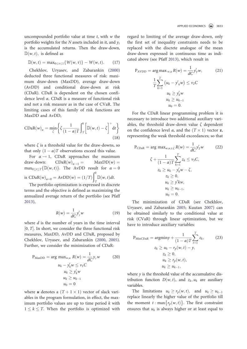
uncompounded portfolio value at time t, with w the
portfolio weights for the N assets included in it, and ytis the accumulated returns. Then the draw-down,
D w; tð Þ; is defined as
D w; tð Þ ¼ max0#τ#1 W w; τð Þf g & W w; tð Þ: (17)
Chekhlov, Uryasev, and Zabarankin (2000)
deducted three functional measures of risk: maxi-
mum draw-down (MaxDD), average draw-down
(AvDD) and conditional draw-down at risk
(CDaR). CDaR is dependent on the chosen confi-
dence level α. CDaR is a measure of functional risk
and not a risk measure as in the case of CVaR. The
limiting cases of this family of risk functions are
MaxDD and AvDD,
CDaR wð Þα ¼ minζ
ζ1
1 & αð ÞT
ð0
T
!
D w; tð Þ & ζ
"þ
dt
# $
(18)
where ζ is a threshold value for the draw-downs, so
that only 1 & αð ÞT observations exceed this value.
For α ! 1, CDaR approaches the maximum
draw-down: CDaR wð Þα!1 ¼ MaxDD wð Þ ¼
max0#t#T D w; tð Þf g: The AvDD result for α ¼ 0
is CDaR wð Þα¼0 ¼ AvDD wð Þ ¼ 1=Tð Þ
ð0
T
D w; tð Þdt.
The portfolio optimization is expressed in discrete
terms and the objective is defined as maximizing the
annualized average return of the portfolio (see Pfaff
2013),
R wð Þ ¼1
dCy0
Tw (19)
where d is the number of years in the time interval
0;T½ +. In short, we consider the three functional risk
measures, MaxDD, AvDD and CDaR, proposed by
Chekhlov, Uryasev, and Zabarankin (2000, 2005).
Further, we consider the minimization of CDaR:
PMaxDD ¼ arg maxw;u R wð Þ ¼1
dCy
Tw (20)
uk & y0kw # v1C
uk , y0kw
uk , uk&1
u0 ¼ 0
where u denotes a T þ 1 - 1ð Þ vector of slack vari-
ables in the program formulation, in effect, the max-
imum portfolio values are up to time period k with
1 # k # T. When the portfolio is optimized with
regard to limiting of the average draw-down, only
the first set of inequality constraints needs to be
replaced with the discrete analogue of the mean
draw-down expressed in continuous time as indi-
cated above (see Pfaff 2013), which result in
PAVDD ¼ arg max w;u R wð Þ ¼1
dCy0Tw; (21)
1
T
X
T
k¼1
uk & y0kw
& '
# v2C
uk , y0kw
uk , uk&1
u0 ¼ 0:
For the CDaR linear programming problem it is
necessary to introduce two additional auxiliary vari-
ables, the threshold draw-down value ζ dependent
on the confidence level α, and the T - 1ð Þ vector z,
representing the weak threshold exceedances; so that
PCDaR ¼ arg maxw;u;z;ζ R wð Þ ¼1
dCy0Tw (22)
ζ þ1
1 & αð ÞT
X
T
k¼1
zk # ν3C;
zk , uk & y0kw & ζ;
zk , 0;
uk , y0kw;
uk , uk&1;
u0 ¼ 0:
The minimization of CDaR (see Chekhlov,
Uryasev, and Zabarankin 2005; Kuutan 2007) can
be obtained similarly to the conditional value at
risk (CVaR) through linear optimization, but we
have to introduce auxiliary variables:
PMinCDaR ¼ argminy þ1
1 & αð ÞT
X
T
t¼1
zk; (23)
zk , uk & rp w; tð Þ & y;
zk , 0;
uk , rp w; tð Þ;
uk , uk&1;
where y is the threshold value of the accumulative dis-
tribution function D w; tð Þ, and zk; uk are auxiliary
variables.
The limitations uk , rp w; tð Þ; and uk , uk&1
replace linearly the higher value of the portfolio till
the moment t : max rp w; tð Þ( )
. The first constraint
ensures that uk is always higher or at least equal to
APPLIED ECONOMICS 3833

the portfolio accumulated return in the moment k,
and the second constraint ensures that uk is always
higher or at least equal to the previous value (see
Kuutan 2007). Before of the optimization process, y
is a free variable, after the optimization process it is
the CDaRα for the MinCDaR portfolio. Thus, if we
minimize the function Hα w; yð Þ, we simultaneously
obtain both values (see Albina Unger 2014).
Minimum tail-dependent portfolio based in Clayton
copulae and low beta strategy
The minimum tail-dependent is derived from a
Clayton copulae. The Clayton copulae belongs to
the family of Archimedean copulae; its one of the
most used in the literature (see Clayton 1978). An
Archimedean generator, or generator, is a continu-
ous decreasing function ψ : 0;1½ $ ! 0; 1½ $, which
complies with ψ 0ð Þ ¼ 1;ψ 1ð Þ :¼ limt!1ψ tð Þ ¼
0; and that is strictly decreasing on
0; inf t : ψ tð Þ ¼ 0f g½ $: The set of all functions is
denoted by Ψ:
An Archimedean generator ψ 2 Ψ is called strict
if ψ tð Þ < 0 for all t 2 0;1½ $. A d-dimensional copu-
lae C is called Archimedean (see Hofert and Scherer
2011) if it allows the representation
C uð Þ ¼ C u;ψð Þ :¼ ψ ψ*1ðu1
!
þ . . . þ ψ*1 udð ÞÞ; u 2 Id
(24)
for some ψ 2 Ψ with inverse ψ*1 : 0; 1½ $ ! 0;1½ $;
where ψ*1 0ð Þ :¼ inf t : ψ tð Þ ¼ 0f g: There are differ-
ent notations for Archimedean copulae. A bivariate
Clayton copulae can be presented so that
C u1; u2ð Þ ¼ ψ*1 ψ u1ð Þ þ ψ u2ð Þð Þ ¼ u*δ1 þ u*δ
2 * 1 !1=δ
(25)
The Clayton copula has the minimum tail-depen-
dence. The coefficient is calculated according to
λl ¼ 2*1=δ. For the bivariate Clayton copulae, the
following simplifications are given:
δ ¼2ρτ
1 * ρτ(26)
θ ¼1
1 * ρτ(27)
where ρτ is the empirical Kendall rank correlation
(see, for example, Genest and Favre 2007).
In addition, we implemented the strategy of lower
beta coefficient (‘Low Beta’); beta (βÞ is the coeffi-
cient used to evaluate systemic risk of an asset in the
CAPM model (see Sharpe 1964; Lintner 1965;
Mossin 1966); it relates the volatility of an asset,
market and the correlation between them.
We select assets whose volatility is less than the
reference market, in absolute terms, for the con-
struction of the beta portfolio. The process to build
the portfolio can be summarized so that, we get the
beta coefficients of each asset such that
βi ¼Cov Ri;Rbð Þ
σ2b
(28)
where the numerator represents the covariance
between assets i and the market b, and the denomi-
nator is the variance of the market.
Then, we select those assets whose β coefficients
and coefficients of tail dependence are below their
respective medians. Finally, we get the weights by
applying an inverse logarithmic scale (this application
can be seen in Pfaff 2013). Both strategies are referred
to as defensive relative to the market (benchmark), as
they are aimed at minimizing systemic risk.
Minimax portfolios based on risk minimization and
optimization of the risk/return ratio
The Minimax model (see Young 1998) aims to mini-
mize the maximum expected loss, thus it is a very
conservative criterion. Formally, when it is applied
to the selection of portfolios, given N assets and t
periods, the model can be presented as a linear
programming problem, such that
minMp;wMp (29)
Mp X
m
j¼1
wjri;j " 0;"i ¼ 1; . . . ; nf g
X
m
j¼1
wjμJ ¼ C
X
m
j¼1
wj ¼ 1
wj % 0;"j 2 1; . . . ; nf g
where Mp is the target value to minimize, which
represents the maximum loss of the portfolio given
a weight vector w, C is a certain minimum level of
return, and μ denote the forecast for the returns
3834 V. M. ADAME ET AL.
vector of m values. In principle, Minimax is consis-
tent with the theory of expected utility in the limit
based on an investor who is very risk averse.
Furthermore, the minimax model is a good approx-
imation to the mean-variance model when the asset
returns follow a multivariate normal distribution.
If we draw the portfolios set for different levels of
C (using an equality rather than inequality), it is
possible to generate the frontier portfolio from
which the optimal risk portfolio can be chosen. It
is possible to estimate the optimal risk/return using
fractional programming as it is described in Charnes
and Cooper (1962), and more recently in Stoyanov,
Rachev, and Fabozzi (2007). The Minimax linear
programming problem can be reformulated, so that
minMp;wbMp (30)
Mp X
m
j¼1
wjri;j " 0;"i ¼ 1; . . . ; nf g
X
m
j¼1
wjμJ ¼ 1
X
m
j¼1
wj ¼ b
b % 0
where b is the multiplier coefficient added to the
optimization problem as a result of transformation
of the risk/return problem. More details can be
found in Charnes and Cooper (1962) for LP (linear
programing), and in Dinkelbach (1967) for NLP
(nonlinear programing).
In summary, we use two types of optimization: the
first optimization is based on risk minimization, and the
second optimization is based on the risk/return ratio.
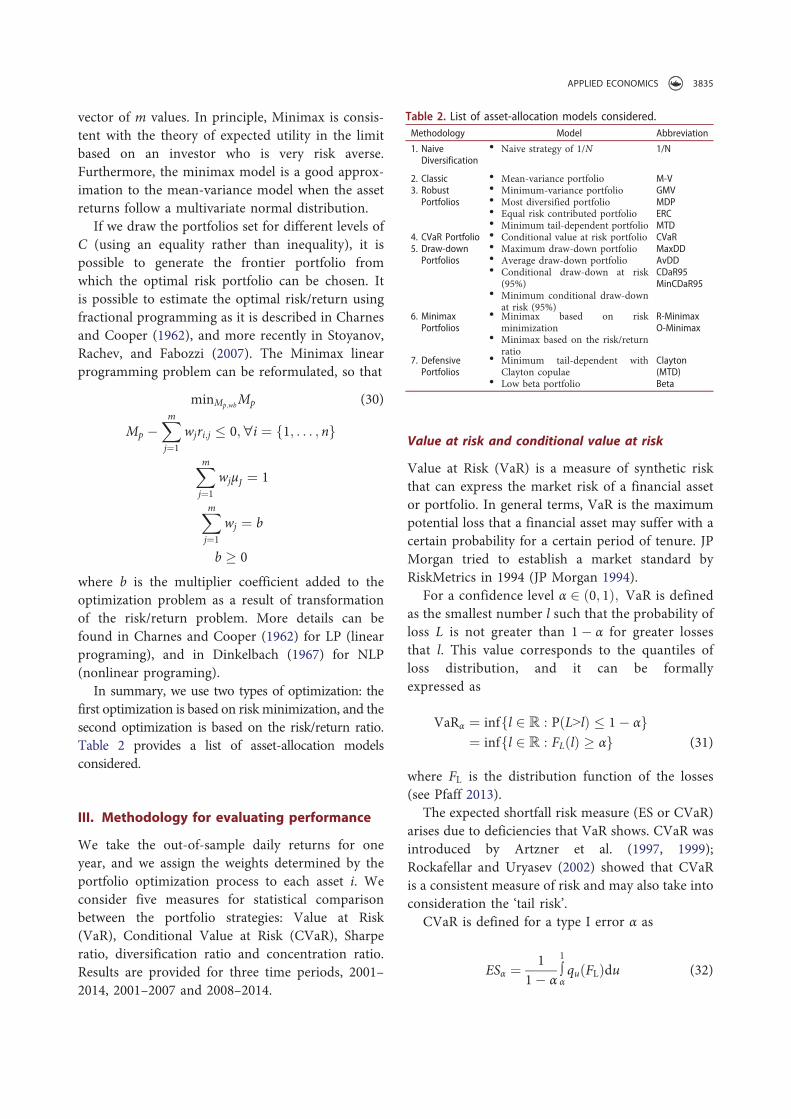
Table 2 provides a list of asset-allocation models
considered.
III. Methodology for evaluating performance
We take the out-of-sample daily returns for one
year, and we assign the weights determined by the
portfolio optimization process to each asset i. We
consider five measures for statistical comparison
between the portfolio strategies: Value at Risk
(VaR), Conditional Value at Risk (CVaR), Sharpe
ratio, diversification ratio and concentration ratio.
Results are provided for three time periods, 2001–
2014, 2001–2007 and 2008–2014.
Value at risk and conditional value at risk
Value at Risk (VaR) is a measure of synthetic risk
that can express the market risk of a financial asset
or portfolio. In general terms, VaR is the maximum
potential loss that a financial asset may suffer with a
certain probability for a certain period of tenure. JP
Morgan tried to establish a market standard by
RiskMetrics in 1994 (JP Morgan 1994).
For a confidence level α 2 0; 1ð Þ; VaR is defined
as the smallest number l such that the probability of
loss L is not greater than 1 α for greater losses
that l. This value corresponds to the quantiles of
loss distribution, and it can be formally
expressed as
VaRα ¼ inf l 2 R : P L>lð Þ " 1 αf g
¼ inf l 2 R : FL lð Þ % αf g (31)
where FL is the distribution function of the losses
(see Pfaff 2013).
The expected shortfall risk measure (ES or CVaR)
arises due to deficiencies that VaR shows. CVaR was
introduced by Artzner et al. (1997, 1999);
Rockafellar and Uryasev (2002) showed that CVaR
is a consistent measure of risk and may also take into
consideration the ‘tail risk’.
CVaR is defined for a type I error α as
ESα ¼1
1 α!1
αqu FLð Þdu (32)
Table 2. List of asset-allocation models considered.
Methodology Model Abbreviation
1. NaiveDiversification
• Naive strategy of 1/N 1/N
2. Classic • Mean-variance portfolio M-V3. RobustPortfolios
• Minimum-variance portfolio• Most diversified portfolio• Equal risk contributed portfolio• Minimum tail-dependent portfolio
GMVMDPERCMTD
4. CVaR Portfolio • Conditional value at risk portfolio CVaR5. Draw-downPortfolios
• Maximum draw-down portfolio• Average draw-down portfolio• Conditional draw-down at risk
(95%)• Minimum conditional draw-down
at risk (95%)
MaxDDAvDDCDaR95MinCDaR95
6. MinimaxPortfolios
• Minimax based on riskminimization
• Minimax based on the risk/returnratio
R-MinimaxO-Minimax
7. DefensivePortfolios
• Minimum tail-dependent withClayton copulae
• Low beta portfolio
Clayton(MTD)Beta
APPLIED ECONOMICS 3835
where qu FLð Þ is the quantile function of loss distri-
bution FL. Therefore ES can be expressed in VaR
terms such that
ESα ¼ 1
1# α
1
α
VaRu Lð Þdu (33)
ES can be interpreted as the VaR average in the
range 1# α; 1ð Þ.
Sharpe ratio
We calculate the out-of-sample annualized Sharpe
ratio for each strategy z. Sharpe ratio is defined as
the sample mean of out-of-sample excess returns
over the risk-free asset μz, divided by their sample
SD σz, such that
Sharpe R ¼ μz
σz: (34)
To test the statistical independence of the Sharpe
ratios for each strategy with respect to benchmark,
we calculate the p-value of the difference, using the
approach suggested by Jobson and Korkie (1981)
after making the correction pointed out in
Memmel (2003), and recently applied in DeMiguel,
Garlappi, and Uppal (2009). So that, given two port-
folios a and b, with mean μa; μb; variance σa; σb, and
covariance σa;b about a sample of size N, its checked
by the test statistic zJK; the null hypothesis that
H0 : μa=σa # μb=σb ¼ 0. This test is based on the
assumption that income is distributed independently
and identically (IID) in time following a normal
distribution, (see Jobson and Korkie 1981; Memmel
2003).
Diversification ratio and concentration ratio
We define diversification ratio (DR) to any portfolio
P as follows:
DR Pð Þ ¼ w0σffiffiffiffiffiffiffiffiffiffiffiffiffi
w0Pw
p : (7)
The numerator is the weighted average volatility
of the single assets, divided by the portfolio volatility
(portfolio SD). From the above equation we derive
the following expression:
DR Pð Þ ¼ 1ffiffiffiffiffiffiffiffiffiffiffiffiffiffiffiffiffiffiffiffiffiffiffiffiffiffiffiffiffiffiffiffi
ρþ CRð Þ # ρCRp (8)
where ρ denotes the volatility-weighted average cor-
relation and CR is the volatility-weighted concentra-
tion ratio. The parameter ρ is defined as
ρ ¼
PNi�j wiσiwjσj
# $
ρijPN
i�j wiσiwjσj
# $ (35)
The concentration ratio (CR) is the normalized
Herfindahl–Hirschmann index (see Hirschman 1964):
CR Pð Þ ¼
PNi¼1 wiσið Þ2
PNi¼1 wiσið Þ2
(36)
IV. Results
In this section, we compare the out-of-sample results
obtained for the various portfolio strategies. For that,
we show the results of the five measures for statistical
comparison between the portfolio strategies, con-
tained in the previous section. The portfolio strategies
results are compared with the Ibex 35 index and the
naive strategy of 1/N. Table A1 in the Appendix
provides descriptive statistics sumarising the beha-
viour during different time perios of the Ibex 35
index and the 15 main models consider in this article.
We take the out-of-sample daily returns for one
year, and we assign the weights determined by the
portfolio optimization process to each asset i con-
sidered, so that we build the portfolio and analyse it
for next year. Therefore, we build portfolios with the
daily returns series of Nt period and they are tested
for the following period, Ntþ1, for
t ¼ 2000; 2001; . . . ; 2013. We have built 14 portfo-
lios for methodological framework, although the
results are aggregated by time periods: 2001–2014,
2001–2007 and 2008–2014.
In the first and second columns of Tables 3–5, we
present the total return (Total Return) and the
annualized return (Annual Return) of each strategy
for the time periods 2001–2014 (Table 3), 2001–2007
(Table 4) and 2008–2014 (Table 5). The value at risk
and the conditional value at risk (1 day) appear in
the third and fourth columns, respectively. The
Sharpe ratio and the p-value of each strategy, includ-
ing the Ibex 35 index, are shown in the fifth column.
We also include the p-value of the difference for
each strategy with respect to Ibex 35 index. In the
last two columns, six and seven, we report the diver-
sification and concentration ratios, respectively.
3836 V. M. ADAME ET AL.
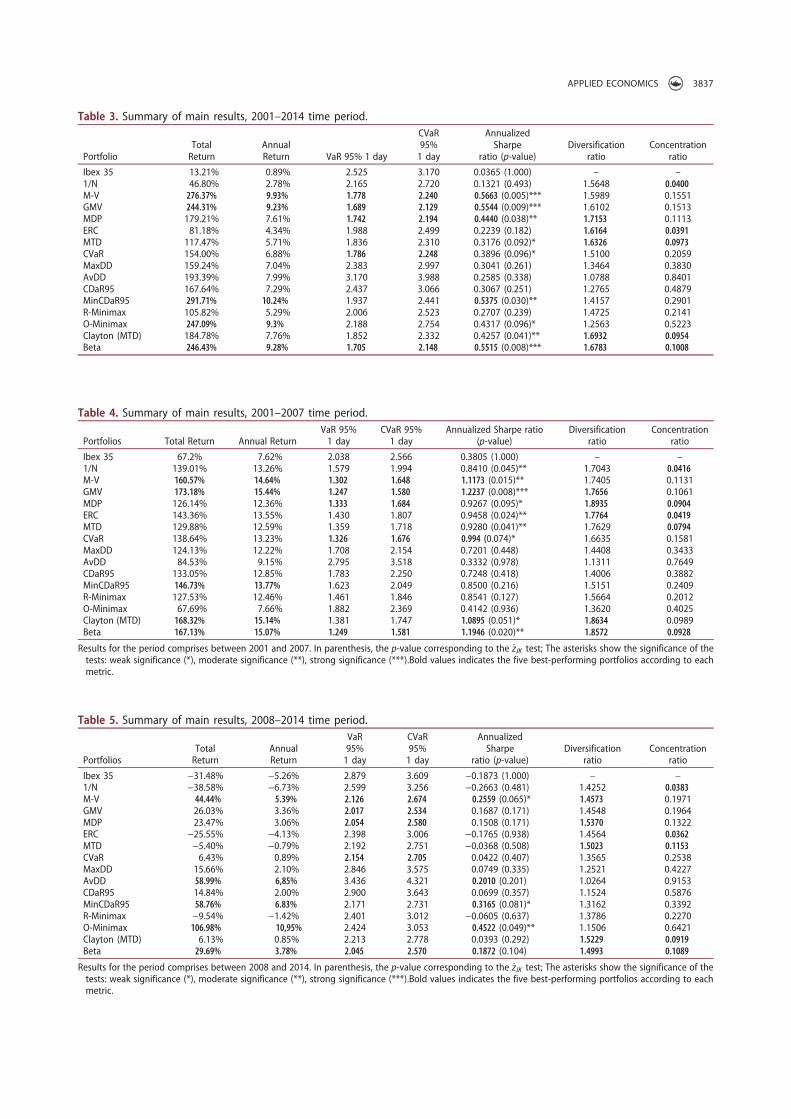
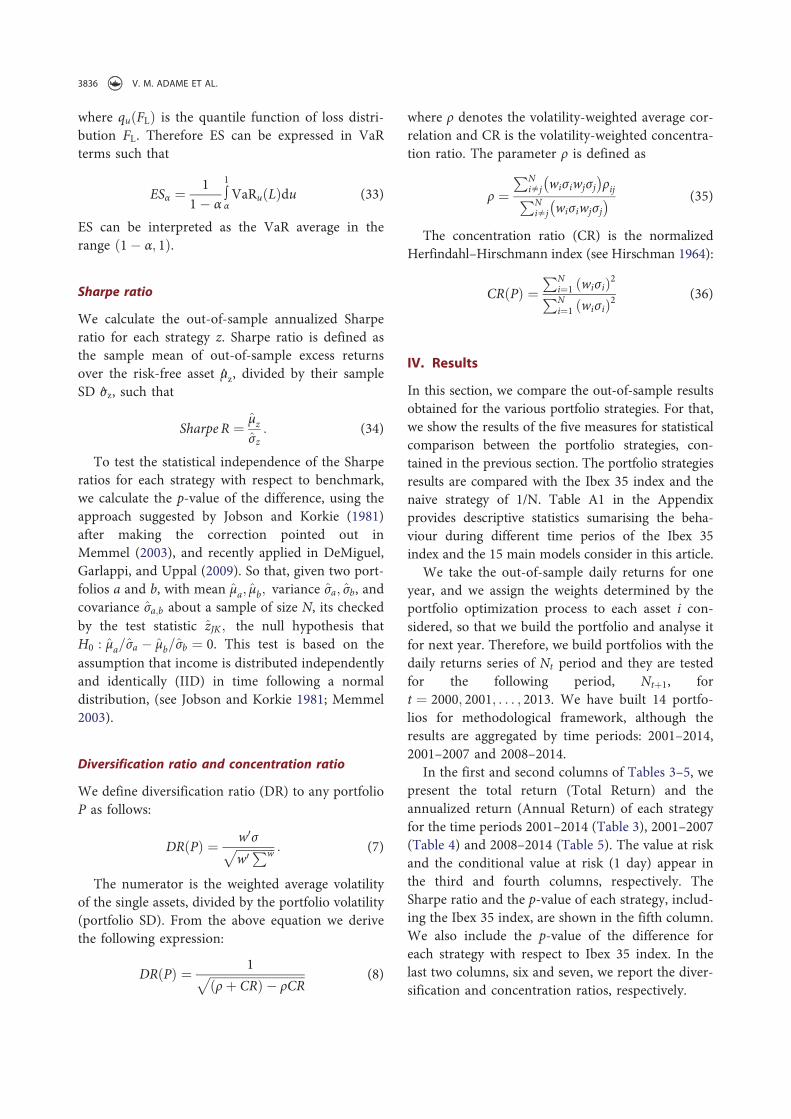
Table 3. Summary of main results, 2001–2014 time period.
PortfolioTotalReturn
AnnualReturn VaR 95% 1 day
CVaR95%1 day
AnnualizedSharpe
ratio (p-value)Diversification
ratioConcentration
ratio
Ibex 35 13.21% 0.89% 2.525 3.170 0.0365 (1.000) – –
1/N 46.80% 2.78% 2.165 2.720 0.1321 (0.493) 1.5648 0.0400
M-V 276.37% 9.93% 1.778 2.240 0.5663 (0.005)*** 1.5989 0.1551GMV 244.31% 9.23% 1.689 2.129 0.5544 (0.009)*** 1.6102 0.1513MDP 179.21% 7.61% 1.742 2.194 0.4440 (0.038)** 1.7153 0.1113ERC 81.18% 4.34% 1.988 2.499 0.2239 (0.182) 1.6164 0.0391
MTD 117.47% 5.71% 1.836 2.310 0.3176 (0.092)* 1.6326 0.0973
CVaR 154.00% 6.88% 1.786 2.248 0.3896 (0.096)* 1.5100 0.2059MaxDD 159.24% 7.04% 2.383 2.997 0.3041 (0.261) 1.3464 0.3830AvDD 193.39% 7.99% 3.170 3.988 0.2585 (0.338) 1.0788 0.8401CDaR95 167.64% 7.29% 2.437 3.066 0.3067 (0.251) 1.2765 0.4879MinCDaR95 291.71% 10.24% 1.937 2.441 0.5375 (0.030)** 1.4157 0.2901R-Minimax 105.82% 5.29% 2.006 2.523 0.2707 (0.239) 1.4725 0.2141O-Minimax 247.09% 9.3% 2.188 2.754 0.4317 (0.096)* 1.2563 0.5223Clayton (MTD) 184.78% 7.76% 1.852 2.332 0.4257 (0.041)** 1.6932 0.0954
Beta 246.43% 9.28% 1.705 2.148 0.5515 (0.008)*** 1.6783 0.1008
Table 4. Summary of main results, 2001–2007 time period.
Portfolios Total Return Annual ReturnVaR 95%1 day
CVaR 95%1 day
Annualized Sharpe ratio(p-value)
Diversificationratio
Concentrationratio
Ibex 35 67.2% 7.62% 2.038 2.566 0.3805 (1.000) – –
1/N 139.01% 13.26% 1.579 1.994 0.8410 (0.045)** 1.7043 0.0416
M-V 160.57% 14.64% 1.302 1.648 1.1173 (0.015)** 1.7405 0.1131GMV 173.18% 15.44% 1.247 1.580 1.2237 (0.008)*** 1.7656 0.1061MDP 126.14% 12.36% 1.333 1.684 0.9267 (0.095)* 1.8935 0.0904
ERC 143.36% 13.55% 1.430 1.807 0.9458 (0.024)** 1.7764 0.0419
MTD 129.88% 12.59% 1.359 1.718 0.9280 (0.041)** 1.7629 0.0794
CVaR 138.64% 13.23% 1.326 1.676 0.994 (0.074)* 1.6635 0.1581MaxDD 124.13% 12.22% 1.708 2.154 0.7201 (0.448) 1.4408 0.3433AvDD 84.53% 9.15% 2.795 3.518 0.3332 (0.978) 1.1311 0.7649CDaR95 133.05% 12.85% 1.783 2.250 0.7248 (0.418) 1.4006 0.3882MinCDaR95 146.73% 13.77% 1.623 2.049 0.8500 (0.216) 1.5151 0.2409R-Minimax 127.53% 12.46% 1.461 1.846 0.8541 (0.127) 1.5664 0.2012O-Minimax 67.69% 7.66% 1.882 2.369 0.4142 (0.936) 1.3620 0.4025Clayton (MTD) 168.32% 15.14% 1.381 1.747 1.0895 (0.051)* 1.8634 0.0989Beta 167.13% 15.07% 1.249 1.581 1.1946 (0.020)** 1.8572 0.0928
Results for the period comprises between 2001 and 2007. In parenthesis, the p-value corresponding to the zJK test; The asterisks show the significance of thetests: weak significance (*), moderate significance (**), strong significance (***).Bold values indicates the five best-performing portfolios according to eachmetric.
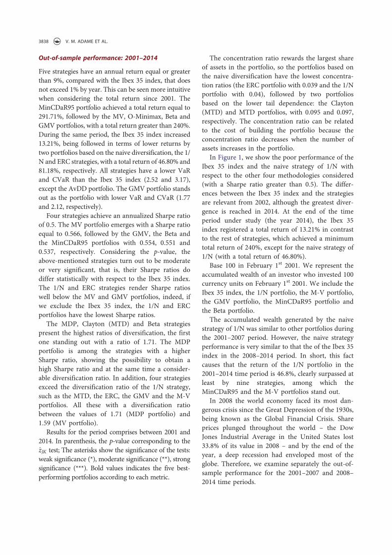
Table 5. Summary of main results, 2008–2014 time period.
PortfoliosTotalReturn
AnnualReturn
VaR95%1 day
CVaR95%1 day
AnnualizedSharpe
ratio (p-value)Diversification
ratioConcentration
ratio
Ibex 35 −31.48% −5.26% 2.879 3.609 −0.1873 (1.000) – –
1/N −38.58% −6.73% 2.599 3.256 −0.2663 (0.481) 1.4252 0.0383
M-V 44.44% 5.39% 2.126 2.674 0.2559 (0.065)* 1.4573 0.1971GMV 26.03% 3.36% 2.017 2.534 0.1687 (0.171) 1.4548 0.1964MDP 23.47% 3.06% 2.054 2.580 0.1508 (0.171) 1.5370 0.1322ERC −25.55% −4.13% 2.398 3.006 −0.1765 (0.938) 1.4564 0.0362
MTD −5.40% −0.79% 2.192 2.751 −0.0368 (0.508) 1.5023 0.1153
CVaR 6.43% 0.89% 2.154 2.705 0.0422 (0.407) 1.3565 0.2538MaxDD 15.66% 2.10% 2.846 3.575 0.0749 (0.335) 1.2521 0.4227AvDD 58.99% 6,85% 3.436 4.321 0.2010 (0.201) 1.0264 0.9153CDaR95 14.84% 2.00% 2.900 3.643 0.0699 (0.357) 1.1524 0.5876MinCDaR95 58.76% 6.83% 2.171 2.731 0.3165 (0.081)* 1.3162 0.3392R-Minimax −9.54% −1.42% 2.401 3.012 −0.0605 (0.637) 1.3786 0.2270O-Minimax 106.98% 10,95% 2.424 3.053 0.4522 (0.049)** 1.1506 0.6421Clayton (MTD) 6.13% 0.85% 2.213 2.778 0.0393 (0.292) 1.5229 0.0919
Beta 29.69% 3.78% 2.045 2.570 0.1872 (0.104) 1.4993 0.1089
Results for the period comprises between 2008 and 2014. In parenthesis, the p-value corresponding to the zJK test; The asterisks show the significance of thetests: weak significance (*), moderate significance (**), strong significance (***).Bold values indicates the five best-performing portfolios according to eachmetric.
APPLIED ECONOMICS 3837
Out-of-sample performance: 2001–2014
Five strategies have an annual return equal or greater
than 9%, compared with the Ibex 35 index, that does
not exceed 1% by year. This can be seen more intuitive
when considering the total return since 2001. The
MinCDaR95 portfolio achieved a total return equal to
291.71%, followed by the MV, O-Minimax, Beta and
GMV portfolios, with a total return greater than 240%.
During the same period, the Ibex 35 index increased
13.21%, being followed in terms of lower returns by
two portfolios based on the naive diversification, the 1/
N and ERC strategies, with a total return of 46.80% and
81.18%, respectively. All strategies have a lower VaR
and CVaR than the Ibex 35 index (2.52 and 3.17),
except the AvDD portfolio. The GMV portfolio stands
out as the portfolio with lower VaR and CVaR (1.77
and 2.12, respectively).
Four strategies achieve an annualized Sharpe ratio
of 0.5. The MV portfolio emerges with a Sharpe ratio
equal to 0.566, followed by the GMV, the Beta and
the MinCDaR95 portfolios with 0.554, 0.551 and
0.537, respectively. Considering the p-value, the
above-mentioned strategies turn out to be moderate
or very significant, that is, their Sharpe ratios do
differ statistically with respect to the Ibex 35 index.
The 1/N and ERC strategies render Sharpe ratios
well below the MV and GMV portfolios, indeed, if
we exclude the Ibex 35 index, the 1/N and ERC
portfolios have the lowest Sharpe ratios.
The MDP, Clayton (MTD) and Beta strategies
present the highest ratios of diversification, the first
one standing out with a ratio of 1.71. The MDP
portfolio is among the strategies with a higher
Sharpe ratio, showing the possibility to obtain a
high Sharpe ratio and at the same time a consider-
able diversification ratio. In addition, four strategies
exceed the diversification ratio of the 1/N strategy,
such as the MTD, the ERC, the GMV and the M-V
portfolios. All these with a diversification ratio
between the values of 1.71 (MDP portfolio) and
1.59 (MV portfolio).
Results for the period comprises between 2001 and
2014. In parenthesis, the p-value corresponding to the
zJK test; The asterisks show the significance of the tests:
weak significance (*), moderate significance (**), strong
significance (***). Bold values indicates the five best-
performing portfolios according to each metric.
The concentration ratio rewards the largest share
of assets in the portfolio, so the portfolios based on
the naive diversification have the lowest concentra-
tion ratios (the ERC portfolio with 0.039 and the 1/N
portfolio with 0.04), followed by two portfolios
based on the lower tail dependence: the Clayton
(MTD) and MTD portfolios, with 0.095 and 0.097,
respectively. The concentration ratio can be related
to the cost of building the portfolio because the
concentration ratio decreases when the number of
assets increases in the portfolio.
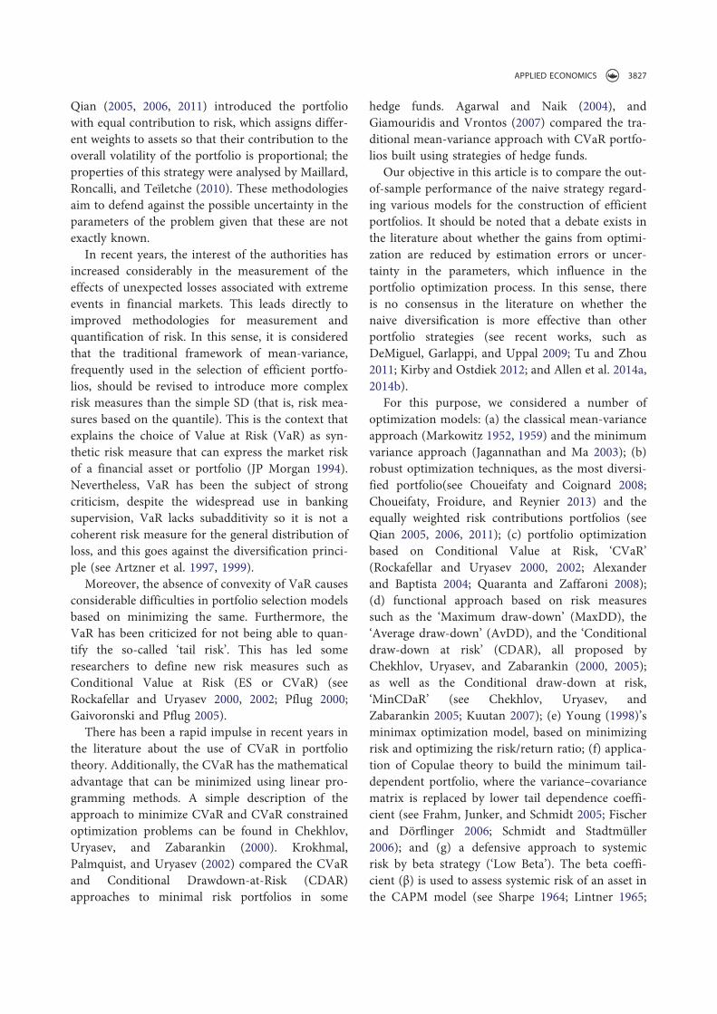
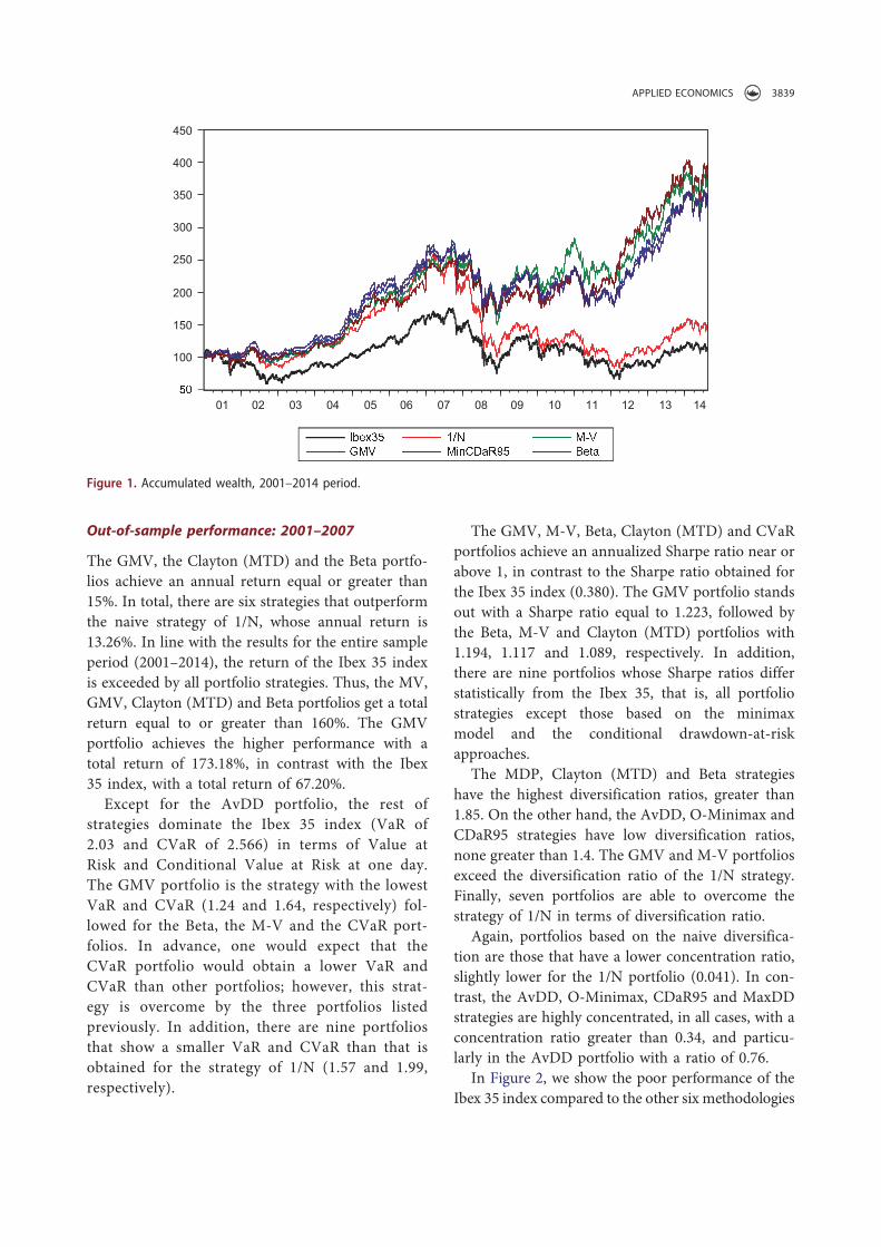
In Figure 1, we show the poor performance of the
Ibex 35 index and the naive strategy of 1/N with
respect to the other four methodologies considered
(with a Sharpe ratio greater than 0.5). The differ-
ences between the Ibex 35 index and the strategies
are relevant from 2002, although the greatest diver-
gence is reached in 2014. At the end of the time
period under study (the year 2014), the Ibex 35
index registered a total return of 13.21% in contrast
to the rest of strategies, which achieved a minimum
total return of 240%, except for the naive strategy of
1/N (with a total return of 46.80%).
Base 100 in February 1st 2001. We represent the
accumulated wealth of an investor who invested 100
currency units on February 1st 2001. We include the
Ibex 35 index, the 1/N portfolio, the M-V portfolio,
the GMV portfolio, the MinCDaR95 portfolio and
the Beta portfolio.
The accumulated wealth generated by the naive
strategy of 1/N was similar to other portfolios during
the 2001–2007 period. However, the naive strategy
performance is very similar to that the of the Ibex 35
index in the 2008–2014 period. In short, this fact
causes that the return of the 1/N portfolio in the
2001–2014 time period is 46.8%, clearly surpassed at
least by nine strategies, among which the
MinCDaR95 and the M-V portfolios stand out.
In 2008 the world economy faced its most dan-
gerous crisis since the Great Depression of the 1930s,
being known as the Global Financial Crisis. Share
prices plunged throughout the world – the Dow
Jones Industrial Average in the United States lost
33.8% of its value in 2008 – and by the end of the
year, a deep recession had enveloped most of the
globe. Therefore, we examine separately the out-of-
sample performance for the 2001–2007 and 2008–
2014 time periods.
3838 V. M. ADAME ET AL.
Out-of-sample performance: 2001–2007
The GMV, the Clayton (MTD) and the Beta portfo-
lios achieve an annual return equal or greater than
15%. In total, there are six strategies that outperform
the naive strategy of 1/N, whose annual return is
13.26%. In line with the results for the entire sample
period (2001–2014), the return of the Ibex 35 index
is exceeded by all portfolio strategies. Thus, the MV,
GMV, Clayton (MTD) and Beta portfolios get a total
return equal to or greater than 160%. The GMV
portfolio achieves the higher performance with a
total return of 173.18%, in contrast with the Ibex
35 index, with a total return of 67.20%.
Except for the AvDD portfolio, the rest of
strategies dominate the Ibex 35 index (VaR of
2.03 and CVaR of 2.566) in terms of Value at
Risk and Conditional Value at Risk at one day.
The GMV portfolio is the strategy with the lowest
VaR and CVaR (1.24 and 1.64, respectively) fol-
lowed for the Beta, the M-V and the CVaR port-
folios. In advance, one would expect that the
CVaR portfolio would obtain a lower VaR and
CVaR than other portfolios; however, this strat-
egy is overcome by the three portfolios listed
previously. In addition, there are nine portfolios
that show a smaller VaR and CVaR than that is
obtained for the strategy of 1/N (1.57 and 1.99,
respectively).
The GMV, M-V, Beta, Clayton (MTD) and CVaR
portfolios achieve an annualized Sharpe ratio near or
above 1, in contrast to the Sharpe ratio obtained for
the Ibex 35 index (0.380). The GMV portfolio stands
out with a Sharpe ratio equal to 1.223, followed by
the Beta, M-V and Clayton (MTD) portfolios with
1.194, 1.117 and 1.089, respectively. In addition,
there are nine portfolios whose Sharpe ratios differ
statistically from the Ibex 35, that is, all portfolio
strategies except those based on the minimax
model and the conditional drawdown-at-risk
approaches.
The MDP, Clayton (MTD) and Beta strategies
have the highest diversification ratios, greater than
1.85. On the other hand, the AvDD, O-Minimax and
CDaR95 strategies have low diversification ratios,
none greater than 1.4. The GMV and M-V portfolios
exceed the diversification ratio of the 1/N strategy.
Finally, seven portfolios are able to overcome the
strategy of 1/N in terms of diversification ratio.
Again, portfolios based on the naive diversifica-
tion are those that have a lower concentration ratio,
slightly lower for the 1/N portfolio (0.041). In con-
trast, the AvDD, O-Minimax, CDaR95 and MaxDD
strategies are highly concentrated, in all cases, with a
concentration ratio greater than 0.34, and particu-
larly in the AvDD portfolio with a ratio of 0.76.
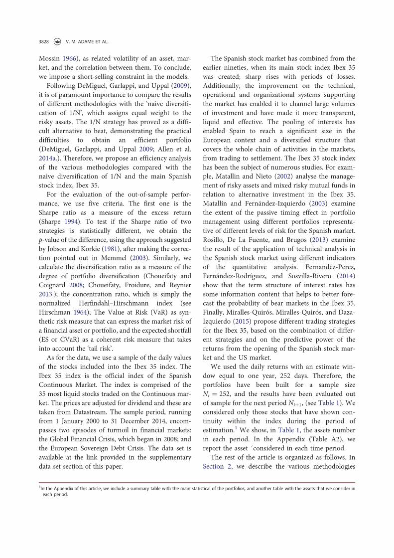
In Figure 2, we show the poor performance of the
Ibex 35 index compared to the other six methodologies
5�
100
150
200
250
300
350
400
450
01 02 03 04 05 06 07 08 09 10 11 12 13 14
I����5 1�� M��
GM� M�� ��5 B��
Figure 1. Accumulated wealth, 2001–2014 period.
APPLIED ECONOMICS 3839

under evaluation (the five portfolios with a higher
Sharpe ratio and the naive strategy of 1/N). As can be
seen, the differences between the Ibex 35 index and the
portfolios began from the middle of 2001. From 2001
to 2007, the Ibex35 index achieved a total return of just
over 67%. Meanwhile, the GMV and MV strategies
had a total return greater than 160%. Even the strategy
of 1/N obtained double return (139.01%) than the Ibex
35 index.
The strategy of 1/N provides a good out-of-sam-
ple performance, especially when it is compared with
the Ibex 35 index. However, the 1/N portfolio is
clearly exceeded by other strategies, not only on
return but also on a higher Sharpe ratio, a lower
VaR and CVaR, and greater diversification ratio. In
short, there are five portfolios that completely dom-
inate, except in concentration ratio, the naive strat-
egy of 1/N, among which the GMV, MV and Beta
portfolios stand out.
Base 100 in February 1st 2001. We represent the
accumulated wealth of an investor who invested 100
currency units on February 1st 2001. We include the
Ibex 35 index, the 1/N portfolio, the M-V portfolio,
the GMV portfolio, the Beta portfolio, the Clayton
(MTD) portfolio and the CVaR portfolio.
In conclusion, the weak out-of-simple perfor-
mance of the 1/N strategy in the time period 2001–
2014 contrasts with the good performance of this
portfolio in the time period 2001–2007; this beha-
viour suggests that the 1/N strategy has been quite
poor during the Global Financial Crisis and
European Sovereign Debt Crisis.
Out-of-sample performance: 2008–2014
Four portfolios achieve an annual return higher than
5% in the 2008–2014 period, providing the
O-Minimax portfolio the greatest return, with an
annual return of around 11%. It is an exceptional
case since the rest of strategies are unable to overcome
such threshold of 5% by year. The return obtained is
well below that achieved in the previous period, where
three portfolios rendered annualized returns above
15%. The Ibex 35 index and the 1/N portfolio are in
the opposite direction, with an annual return drop of
5.26% and 6.73%, respectively. Taking this into con-
sideration, the relative performance of other strategies
is not as poor as it might seem a priori.
If we consider the total return for the period, the
O-Minimax portfolio obtains a return of 100%, fol-
lowed for the AVDD portfolio with a 58.99%, the
MinCDaR95 portfolio with 58.76% and the MV
portfolio with a 44.44% of total return. Meanwhile,
on the opposite side the 1/N portfolio stands out
with a total return of −38.58% and the Ibex 35 index
with a total return of −31.48%. So the strategy of 1/N
4�
80
120
160
200
240
280
320
2001 2002 2003 2004 2005 2006 2007
������ ��� ���
��� �� ! C"!# $% &�'()
C�!*
Figure 2. Accumulated wealth, 2001–2007 time period.
3840 V. M. ADAME ET AL.

obtained negative returns even higher than those
obtained by the Ibex 35 index.
Regarding the Value at Risk and Conditional
Value at Risk associate with each strategy, it is
again the GMV portfolio which has a lower VaR
and CVaR with 2.01 and 2.53, respectively. The
GMV portfolio is followed by the Beta, MDP, MV
and CVaR portfolios, in no case, with a VaR and
CVaR higher than 2.2 and 2.8. These are good
results if we compare them with the Ibex 35 index
(2.879 and 3.256) and the 1/N strategy (2.599 and
3.256). In this regard, 11 out of the 14 portfolios
have a lower VaR and CVaR with respect to the Ibex
35 index and the 1/N strategy.
All strategies, except the 1/N portfolio (−0266),
obtained Sharpe ratios higher than that for the Ibex
35 index. However, they are only three strategies that
statistically exceed the Sharpe ratio of the Ibex 35
index; this is because the covariance between the port-
folio and the index is very high. The O-Minimax
portfolio has the highest Sharpe ratio (0.452), and the
difference from the Ibex 35 index is moderately sig-
nificant. Regarding the other two portfolios: the
MinCDaR95 (0.315) and the MV (0.255) portfolios,
both present a relatively high Sharpe ratio, although in
both cases the difference is weakly significant.
The MDP, Clayton (MTD) and MTD strategies
have the highest diversification ratios, the MDP with
a remarkable ratio of 1.53, nevertheless somewhat
lower than the value of the 2001–2007 time period,
highlighting the highest correlation between asset
returns in the portfolio during the 2008–2014 period.
Again, the AvDD, CDaR95 and MaxDD portfolios
have the lowest diversification ratio. In total, there
are seven strategies that exceed the diversification
ratio of the 1/N portfolio (1.42), including the Beta
(1,499), MV (1,457) and GMV(1.454) portfolios.
The ERC and 1/N portfolios have the lowest con-
centration ratios, with 0.036 and 0.038, respectively.
The concentration ratio is slightly lower than that in
the 2001–2007 time period due to an increase in the
assets number (see Table 1). In contrast, the AVDD,
O-Minimax and CDaR95 strategies present a higher
concentration ratio, in all cases with a concentration
ratio greater than 0.58. This increase can be
explained by the higher correlation between asset
returns. This fact is widely investigated in recent
papers as Moldovan (2011), for the New York,
London and Tokyo index; and in Ahmad et al.
(2013), for the contagion between financial markets.
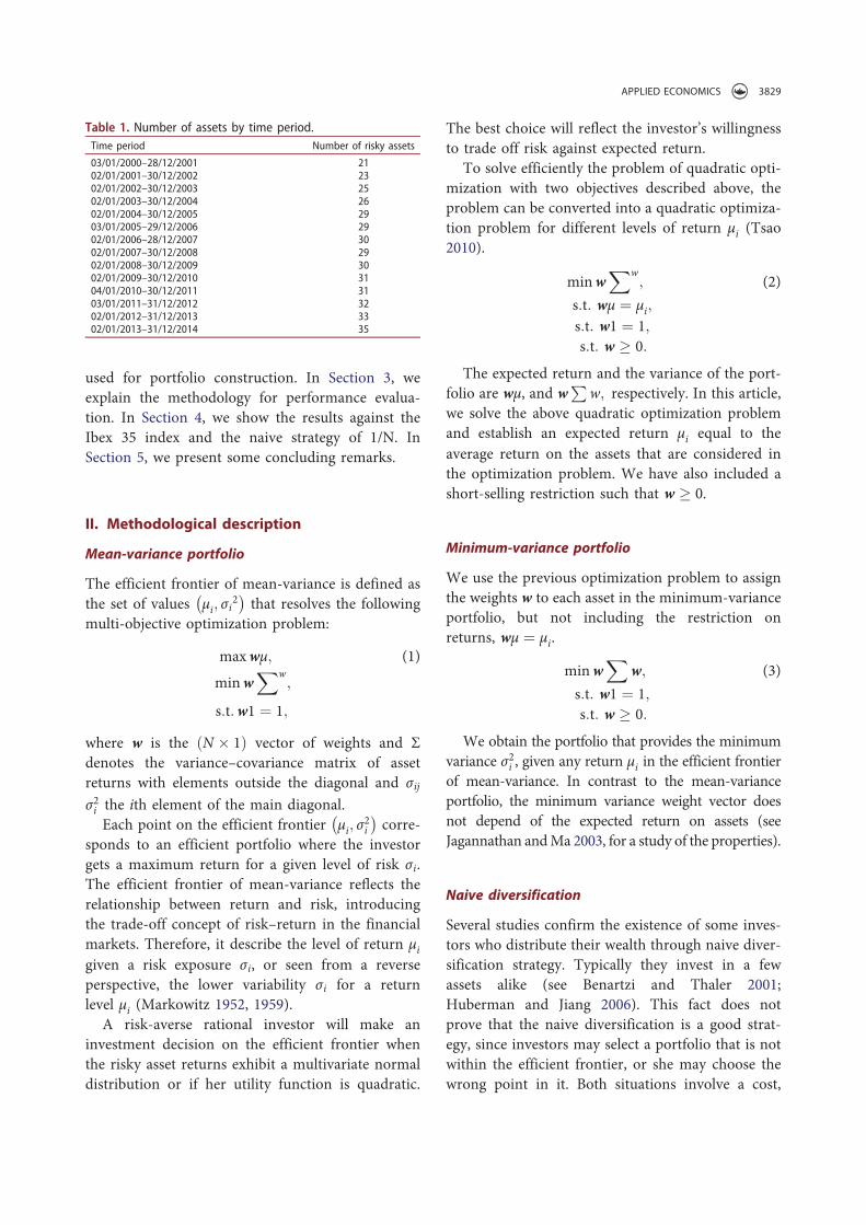
In Figure 3, we show the poor performance of the
Ibex 35 index and the 1/N portfolio compared to the
0
40
80
120
160
200
240
2008 2009 2010 2011 2012 2013 2014
+,-./2 367 89:
O98;<;=>. 8;<?@>AD2 E-F>
Figure 3. Accumulated wealth, 2008–2014 time period.
Accumulated wealth in the 2008–2014 time period. Base 100 in January 2nd 2008. We represent the accumulated wealth of aninvestor who invested 100 currency units on January 2nd 2008. We include the Ibex 35 index, the 1/N portfolio, the M-V portfolio,the O-Minimax portfolio, the MinCDaR95 portfolio, and the Beta portfolio.
APPLIED ECONOMICS 3841
other four methodologies under scrutiny (three port-
folios with Sharpe ratio significantly different to the
Ibex 35 index and the Beta portfolio, which are
almost significant).
The differences between the 1/N portfolio and
the rest of portfolios began from 2008. The 1/N
portfolio performance is worse than the Ibex 35
index, in terms of total return (−38.58%).
Meanwhile and during this period, the Ibex 35
index performance has been quite poor, with a
total return of −31.48% and annualized Sharpe
ratio of −0.187; in contrast with the performance
of the O-Minimax, the MinCDaR95, the MV and
the Beta portfolios, the O-Minimax standing out
with a total return of 106.98% and annualized
Sharpe ratio of 0.452.
The 1/N portfolio performance before and during
the Global Financial Crisis and European sovereign
debt crisis indicates that this strategy has a good
behaviour when the market trend is bullish and
vice versa when it is bearish. The increase in the
correlation between assets has adversely affected
the 1/N portfolio performance during the period
2008–2014.
V. Concluding remarks
In this article, we have examined 15 asset allocation
models in the main Spanish stock market using the
Ibex 35 index. We have compared the total returns,
Sharpe ratios, VaR and CVaR, and the diversifica-
tion and concentration ratios of each portfolio strat-
egy. We have analysed the performance for the daily
returns over a sample of 14 years, divided into two
sub-samples of seven years each one, whose purpose
is to test the robustness of the results in periods of
high and low correlations between assets and with a
market characterized by many bullish and bearish
trends.
We have found that the Sharpe ratio of the mean-
variance (MV) and the minimum variance (GMV)
strategies are higher compared to the naive strategy
of 1/N and the Ibex 35 index, in the 2001–2014
period. All models achieved a Sharpe ratio greater
than the Ibex 35 index during the 2001–2014 period,
although only nine strategies are statistically differ-
ent from it.
Regarding the total return for the 2001–2014 time
period, the MinCDaR95 portfolio is found to deliver
higher returns, followed for the mean-variance, the
Minimax optimization based on risk/return ratio,
the low beta and the minimum variance strategies.
All these gave returns five times greater than those
derived from the naive strategy of 1/N.
The performance of the naive strategy of 1/N is
found not to be much different from other strategies
in the 2001–2007 period, although it is surpassed by
five models, except in concentration ratio, among
which are the mean-variance (M-V) and the mini-
mum variance (GMV) portfolios.
We observed that the 1/N strategy performance is
worse that the Ibex 35 index in the 2008–2014 per-
iod. It is from 2008 when we detected divergences
between the naive strategy of 1/N and the other
strategies. Our findings suggest that the 1/N portfo-
lio seems to show the worst performance during the
Global Financial Crisis and the European sovereign
debt crisis (that is, a time period characterized by a
higher correlation between financial assets and
downtrends in the markets). Furthermore, except
the O-Minimax portfolio, other strategies are found
to outperform the naive strategy of 1/N in a lower
VaR and CVaR, and a higher diversification ratio.
However, we found that the 1/N portfolio has a
lower degree of concentration, although it is to be
expected since it includes all the assets that make up
the Ibex 35 index. A large number of strategies have
been found to produce a better performance than
the Ibex 35 index and the naive strategy of 1/N. We
have shown that most of strategies outperform better
than both the Ibex35 index and the 1/N strategy,
various portfolio strategies achieving higher return,
greater Sharpe ratio, greater diversification ratio and
lower VaR and CVaR than those associated with the
naive strategy of 1/N and the Ibex 35 index.
In addition, our empirical results indicate that
there are several strategies that do not depend on
the expected assets return to assign weights (such as
the GMV, the ERC, the MDP and the MTD strate-
gies) that are also able to overcome the naive strat-
egy of 1/N. Nevertheless, the Markowitz mean-
variance portfolio with short-selling constraint is
found to be the only strategy that achieves a
Sharpe ratio statistically different to the Ibex 35 in
the two time periods analysed (2001–2007 and
2008–2014). In view of the encouraging results of
this article, we suggest that the mean-variance, mini-
mum-variance and conditional draw-down at risk
3842 V. M. ADAME ET AL.
(95%) portfolios could be used, at least as a first
reference, when analysing the behaviour of the
main Spanish stock market.
All in all, the results of our analysis are not con-
sistent with those presented in DeMiguel, Garlappi,
and Uppal (2009) and Allen et al. (2014a); although
these are in line with those of Kirby and Ostdiek
(2012) and Allen et al. (2014b) for the hedge fund
indices. Thus, although in all empirical works the
results obtained have to be taken with some degree
of caution (since they are based on a particular index
over a certain time period), our findings lead us to
infer that the naive strategy of 1/N can provide good
results during some episodes, being always exceeded
by several portfolio optimization models.
Acknowledgements
The authors thank the insightful comments of two anon-
ymous referees and the editor that have helped to substan-
tially improve this article. Responsibility for any remaining
errors rests with the authors.
Disclosure statement
No potential conflict of interest was reported by the authors.
Funding
This work is supported by the Government of Spain [grant
number ECO2011-23189].
ORCID
Víctor M. Adame http://orcid.org/0000-0002-9338-081X
Simon Sosvilla-Rivero http://orcid.org/0000-0003-2084-
0640
References
Agarwal, V., and N. Y. Naik. 2004. “Risks and Portfolio
Decisions Involving Hedge Funds.” Review of Financial
Studies 17 (1): 63–98. doi:10.1093/rfs/hhg044.
Ahmad, W., S. Sehgal, and N. R. Bhanumurthy. 2013.
“Eurozone Crisis and BRIICKS Stock Markets: Contagion
or Market Interdependence?” Economic Modelling 33: 209–
225. doi:10.1016/j.econmod.2013.04.009.
Alexander, G. J., and A. M. Baptista. 2004. “A Comparison of
Var and Cvar Constraints on Portfolio Selection with the
Mean-Variance Model.” Management Science 50 (9):
1261–1273. doi:10.1287/mnsc.1040.0201.
Allen, D., M. McAleer, S. Peiris, and A. Singh 2014b. Hedge
Fund Portfolio Diversification Strategies across the GFC.
Tinbergen Institute Discussion Paper Series, No. TI
14-151/III.
Allen, D., M. McAleer, R. Powell, and A. Singh. 2014a.
European Market Portfolio Diversification Strategies
across the GFC. Tinbergen Institute Discussion Paper
Series, No. TI 14-134/III.
Andersson, F., H. Mausser, D. Rosen, and S. Uryasev. 2001.
“Credit Risk Optimization with Conditional Value-At-
Risk Criterion.” Mathematical Programming 89 (2): 273–
291. doi:10.1007/PL00011399.
Artzner, P., F. Delbaen, J. Eber, and D. Heath. 1997.
“Thinking Coherently.” Risk 10: 68–71.
Artzner, P., F. Delbaen, J.-M. Eber, and D. Heath. 1999.
“Coherent Measures of Risk.” Mathematical Finance 9
(3): 203–228. doi:10.1111/mafi.1999.9.issue-3.
Benartzi, S., and R. H. Thaler. 2001. “Naive Diversification
Strategies in Defined Contribution Saving Plans.”
American Economic Review 91 (1): 79–98. doi:10.1257/
aer.91.1.79.
Boubaker, H., and N. Sghaier. 2013. “Portfolio Optimization
in the Presence of Dependent Financial Returns with Long
Memory: A Copula Based Approach.” Journal of Banking
and Finance 37 (2): 361–377. doi:10.1016/j.
jbankfin.2012.09.006.
Brennan, M. J., and W. N. Torous. 1999. “Individual
Decision Making and Investor Welfare.” Economic Notes
28 (2): 119–143. doi:10.1111/ecno.1999.28.issue-2.
Chan, L. K., J. Karceski, and J. Lakonishok. 1999. “On
Portfolio Optimization: Forecasting Covariances and
Choosing the Risk Model.” Review of Financial Studies
12 (5): 937–974. doi:10.1093/rfs/12.5.937.
Charnes, A., and W. W. Cooper. 1962. “Programming with
Linear Fractional Functionals.” Naval Research Logistics
Quarterly 9 (3–4): 181–186. doi:10.1002/(ISSN)1931-9193.
Chekhlov, A., S. Uryasev, and M. Zabarankin. 2005.
“Drawdown Measure in Portfolio Optimization.”
International Journal of Theoretical and Applied Finance
8 (01): 13–58. doi:10.1142/S0219024905002767.
Chekhlov, A., S. P. Uryasev, and M. Zabarankin 2000.
Portfolio Optimization with Drawdown Constraints.
Research Report 2000-5. Gainesville: Department of
Industrial and Systems Engineering, University of Florida.
Chopra, V. K. 1993. “Improving Optimization.” The Journal
of Investing 2 (3): 51–59. doi:10.3905/joi.2.3.51.
Choueifaty, Y., and Y. Coignard. 2008. “Toward Maximum
Diversification.” The Journal of Portfolio Management 35
(1): 40–51. doi:10.3905/JPM.2008.35.1.40.
Choueifaty, Y., T. Froidure, and J. Reynier. 2013. “Properties
of the Most Diversified Portfolio.” Journal of Investment
Strategies 2 (2): 49–70.
Clayton, D. G. 1978. “A Model for Association in Bivariate
Life Tables and Its Application in Epidemiological
Studies of Familial Tendency in Chronic Disease
Incidence.” Biometrika 65 (1): 141–151. doi:10.1093/bio-
met/65.1.141.
APPLIED ECONOMICS 3843
DeMiguel, V., L. Garlappi, and R. Uppal. 2009. “Optimal
versus Naive Diversification: How Inefficient Is the 1/N
Portfolio Strategy?” Review of Financial Studies 22 (5):
1915–1953. doi:10.1093/rfs/hhm075.
DeMiguel, V., and F. J. Nogales. 2009. “Portfolio Selection
with Robust Estimation.” Operations Research 57 (3): 560–
577. doi:10.1287/opre.1080.0566.
Dinkelbach, W. 1967. “On Nonlinear Fractional
Programming.” Management Science 13 (7): 492–498.
doi:10.1287/mnsc.13.7.492.
Fernandez-Perez, A., F. Fernández-Rodríguez, and S.Sosvilla-Rivero. 2014. “The Term Structure of InterestRates as Predictor of Stock Returns: Evidence for theIBEX 35 during a Bear Market.” International Review of
Economics and Finance 31: 21–33. doi:10.1016/j.iref.2013.12.004.
Fischer, M. J., and M. Dörflinger 2006. A Note on A Non-Parametric Tail Dependence Estimator.Diskussionspapiere, No. 76/2006. Friedrich-Alexander-Universität Erlangen-Nürnberg, Lehrstuhl für Statistikund Ökonometrie.
Frahm, G., M. Junker, and R. Schmidt. 2005. “Estimating theTail-Dependence Coefficient: Properties and Pitfalls.”Insurance: Mathematics and Economics 37 (1): 80–100.
Frost, P. A., and J. E. Savarino. 1988. “For BetterPerformance: Constrain Portfolio Weights.” The Journal
of Portfolio Management 15 (1): 29–34. doi:10.3905/jpm.1988.409181.
Gaivoronski, A. A., and G. Pflug. 2005. “Value-At-Risk inPortfolio Optimization: Properties and ComputationalApproach.” Journal of Risk 7 (2): 1–31.
Genest, C., and A.-C. Favre. 2007. “Everything You AlwaysWanted to Know about Copula Modeling but Were Afraidto Ask.” Journal of Hydrologic Engineering 12 (4): 347–368.doi:10.1061/(ASCE)1084-0699(2007)12:4(347).
Giamouridis, D., and I. D. Vrontos. 2007. “Hedge FundPortfolio Construction: A Comparison of Static andDynamic Approaches.” Journal of Banking and Finance
31 (1): 199–217. doi:10.1016/j.jbankfin.2006.01.002.Harris, R. D., and M. Mazibas. 2013. “Dynamic Hedge Fund
Portfolio Construction: A Semi-Parametric Approach.”Journal of Banking and Finance 37 (1): 139–149.doi:10.1016/j.jbankfin.2012.08.017.
Hirschman, A. O. 1964. “The Paternity of an Index.”American Economic Review 54 (5): 761–762.
Hofert, M., and M. Scherer. 2011. “CDO Pricing with NestedArchimedean Copulas.” Quantitative Finance 11 (5): 775–787. doi:10.1080/14697680903508479.
Huberman, G., and W. Jiang. 2006. “Offering versus Choicein 401 (K) Plans: Equity Exposure and Number of Funds.”The Journal of Finance 61 (2): 763–801. doi:10.1111/jofi.2006.61.issue-2.
Jagannathan, R., and T. Ma. 2003. “Risk Reduction in LargePortfolios: Why Imposing the Wrong Constraints Helps.”The Journal of Finance 58 (4): 1651–1683. doi:10.1111/jofi.2003.58.issue-4.
Jobson, J. D., and B. M. Korkie. 1981. “PerformanceHypothesis Testing with the Sharpe and TreynorMeasures.” The Journal of Finance 36 (4): 889–908.doi:10.1111/j.1540-6261.1981.tb04891.x.
Jorion, P. 1991. “Bayesian and CAPM Estimators of theMeans: Implications for Portfolio Selection.” Journal of
Banking and Finance 15 (3): 717–727. doi:10.1016/0378-4266(91)90094-3.
Kirby, C., and B. Ostdiek. 2012. “It’s All in the Timing:Simple Active Portfolio Strategies that Outperform NaiveDiversification.” Journal of Financial and Quantitative
Analysis 47 (02): 437–467. doi:10.1017/S0022109012000117.
Krokhmal, P., J. Palmquist, and S. Uryasev. 2002. “PortfolioOptimization with Conditional Value-At-Risk Objectiveand Constraints.” Journal of Risk 4: 43–68.
Kuutan, E. 2007. “Portfolio Optimization Using ConditionalValue-At-Risk and Conditional Drawdown-At-Risk.”Doctoral diss., University of Toronto.
Lintner, J. 1965. “The Valuation of Risk Assets and theSelection of Risky Investments in Stock Portfolios andCapital Budgets.” The Review of Economics and Statistics
47 (1): 13–37. doi:10.2307/1924119.Maillard, S., T. Roncalli, and J. Teïletche. 2010. “The
Properties of Equally Weighted Risk ContributionPortfolios.” The Journal of Portfolio Management 36 (4):60–70. doi:10.3905/jpm.2010.36.4.060.
Markowitz, H. 1952. “Portfolio Selection.” The Journal of
Finance 7 (1): 77–91.Markowitz, H. 1959. Portfolio Selection: Efficient
Diversification of Investments. New York: Basil Blackwall.Matallín, J. C., and A. Fernández-Izquierdo. 2003. “Passive
Timing Effect in Portfolio Management.” Applied
Economics 35 (17): 1829–1837. doi:10.1080/0003684032000150404.
Matallin, J. C., and L. Nieto. 2002. “Mutual Funds as anAlternative to Direct Stock Investment: A CointegrationApproach.” Applied Financial Economics 12 (10): 743–750.doi:10.1080/09603100110038693.
Memmel, C. 2003. “Performance Hypothesis Testing with theSharpe Ratio: The Case of Hedge Funds.” Finance
Research Letters 10 (4): 196–208.Miralles-Quirós, J. L., M. M. Miralles-Quirós, and J. Daza-
Izquierdo. 2015. “Intraday Patterns and Trading Strategiesin the Spanish Stock Market.” Applied Economics 47 (1):88–99. doi:10.1080/00036846.2014.962224.
Moldovan, I. 2011. “Stock Markets Correlation: Before andduring the Crisis Analysis.” Theoretical and Applied
Economics 8 (8): 111–122.Morgan, J. P. 1994. RiskMetrics, Technical Document. New
York: Morgan Guaranty Trust Company.Mossin, J. 1966. “Equilibrium in a Capital Asset Market.”
Econometrica 34 (4): 768–783. doi:10.2307/1910098.Pástor, Ľ. 2000. “Portfolio Selection and Asset Pricing
Models.” The Journal of Finance 55 (1): 179–223.doi:10.1111/jofi.2000.55.issue-1.
3844 V. M. ADAME ET AL.

Pástor, Ľ., and R. F. Stambaugh. 2000. “Comparing Asset
Pricing Models: An Investment Perspective.” Journal of
Financial Economics 56 (3): 335–381. doi:10.1016/S0304-
405X(00)00044-1.
Pfaff, B. 2013. Financial Risk Modelling and Portfolio
Optimization with R. Chichester: John Wiley & Sons.
Pflug, G. C. 2000. “Some Remarks on the Value-At-Risk and
the Conditional Value-At-Risk.” In Probabilistic
Constrained Optimization, edited by Uryasev, S. P., 272–
281. New York: Springer US.
Qian, E. 2005. Risk Parity Portfolios: Efficient Portfolios
through True Diversification. Boston, MA: Panagora
Asset Management.
Qian, E. 2006. “On the Financial Interpretation of Risk
Contribution: Risk Budgets Do Add Up.” Journal of
Investment Management 4 (4): 1–11.
Qian, E. 2011. “Risk Parity and Diversification.” The Journal
of Investing 20 (1): 119–127. doi:10.3905/joi.2011.20.1.119.
Quaranta, A. G., and A. Zaffaroni. 2008. “Robust
Optimization of Conditional Value at Risk and Portfolio
Selection.” Journal of Banking and Finance 32 (10): 2046–
2056. doi:10.1016/j.jbankfin.2007.12.025.
Rockafellar, R. T., and S. Uryasev. 2000. “Optimization of
Conditional Value-At-Risk.” Journal of Risk 2: 21–42.
Rockafellar, R. T., and S. Uryasev. 2002. “Conditional Value-
At-Risk for General Loss Distributions.” Journal of
Banking and Finance 26 (7): 1443–1471. doi:10.1016/
S0378-4266(02)00271-6.
Rockafellar, R. T., S. Uryasev, and M. Zabarankin. 2006.
“Generalized Deviations in Risk Analysis.” Finance and
Stochastics 10 (1): 51–74. doi:10.1007/s00780-005-0165-8.
Rosillo, R., D. De La Fuente, and J. A. L. Brugos. 2013.
“Technical Analysis and the Spanish Stock Exchange:
Testing the RSI, MACD, Momentum and Stochastic
Rules Using Spanish Market Companies.” Applied
Economics 45 (12): 1541–1550. doi:10.1080/
00036846.2011.631894.
Schmidt, R., and U. Stadtmüller. 2006. “Non-parametric
Estimation of Tail Dependence.” Scandinavian Journal of
Statistics 33 (2): 307–335. doi:10.1111/j.1467-
9469.2005.00483.x.
Sharpe, W. F. 1964. “Capital Asset Prices: A Theory of
Market Equilibrium under Conditions of Risk.” The
Journal of Finance 19 (3): 425–442.
Sharpe, W. F. 1994. “The Sharpe Ratio.” The Journal of
Portfolio Management 21 (1): 49–58. doi:10.3905/
jpm.1994.409501.
Sklar, M. 1959. “Fonctions de répartition à n dimensions et
leurs marges.” Université Paris 8: 229–231.
Stoyanov, S. V., S. T. Rachev, and F. J. Fabozzi. 2007.
“Optimal Financial Portfolios.” Applied Mathematical
Finance 14 (5): 401–436. doi:10.1080/13504860701255292.
Tsao, C.-Y. 2010. “Portfolio Selection Based on the Mean-
Var Efficient Frontier.” Quantitative Finance 10 (8): 931–
945. doi:10.1080/14697681003652514.
Tu, J., and G. Zhou. 2011. “Markowitz Meets Talmud: A
Combination of Sophisticated and Naive Diversification
Strategies.” Journal of Financial Economics 99 (1): 204–
215. doi:10.1016/j.jfineco.2010.08.013.
Unger, A. 2014. The Use of Risk Budgets in Portfolio
Optimization. Bremen: Springer Gabler.
Xing, X., J. Hu, and Y. Yang. 2014. “Robust Minimum
Variance Portfolio with L-Infinity Constraints.” Journal
of Banking and Finance 46: 107–117. doi:10.1016/j.
jbankfin.2014.05.004.
Young, M. R. 1998. “A Minimax Portfolio Selection Rule
with Linear Programming Solution.” Management
Science 44 (5): 673–683. doi:10.1287/mnsc.44.5.673.
APPLIED ECONOMICS 3845
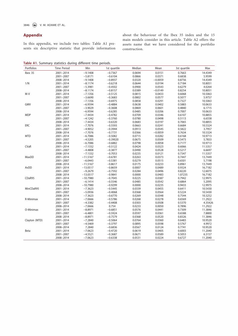
Appendix
In this appendix, we include two tables: Table A1 pre-
sents six descriptive statistic that provide information
about the behaviour of the Ibex 35 index and the 15
main models consider in this article. Table A2 offers the
assets name that we have considered for the portfolio
construction.
Table A1. Summary statistics during different time periods.
Portfolios Time Period Min 1st quartile Median Mean 3st quartile Max
Ibex 35 2001–2014 −9.1408 −0.7367 0.0694 0.0151 0.7663 14.43492001–2007 −5.8171 −0.6104 0.0866 0.0371 0.6838 5.95992008–2014 −9.1408 −0.8937 0.0320 −0.0059 0.8756 14.4349
1/N 2001–2014 −8.1174 −0.6218 0.0644 0.0194 0.7184 10.80512001–2007 −5.3981 −0.4502 0.0900 0.0543 0.6279 4.02642008–2014 −8.1174 −0.8157 0.0389 −0.0149 0.8254 10.8051
M-V 2001–2014 −7.1356 −0.5125 0.0815 0.0433 0.6068 10.50632001–2007 −3.6690 −0.3683 0.0802 0.0577 0.5077 5.97572008–2014 −7.1356 −0.6975 0.0858 0.0291 0.7327 10.5063
GMV 2001–2014 −6.9594 −0.4884 0.0638 0.0402 0.5883 10.06332001–2007 −3.9029 −0.3608 0.0869 0.0601 0.4840 6.17152008–2014 −6.9594 −0.6285 0.0485 0.0206 0.7007 10.0633
MDP 2001–2014 −7.4434 −0.4782 0.0709 0.0346 0.6107 10.88552001–2007 −4.1242 −0.3760 0.0780 0.0498 0.5113 6.65582008–2014 −7.4434 −0.6320 0.0683 0.0197 0.7065 10.8855
ERC 2001–2014 −7.7076 −0.5593 0.0663 0.0241 0.6684 10.53242001–2007 −4.9052 −0.3944 0.0913 0.0545 0.5822 3.79572008–2014 −7.7076 −0.7731 0.0366 −0.0059 0.7634 10.5324
MTD 2001–2014 −6.7086 −0.5082 0.0715 0.0282 0.6168 10.97132001–2007 −4.5205 −0.39020 0.0675 0.0509 0.5473 5.78332008–2014 −6.7086 −0.6882 0.0798 0.0058 0.7177 10.9713
CVaR 2001–2014 −7.1332 −0.5122 0.0424 0.0323 0.6066 11.53572001–2007 −4.4808 −0.3877 0.0490 0.0528 0.5217 6.66972008–2014 −7.1332 −0.7053 0.0235 0.0121 0.7347 11.5357
MaxDD 2001–2014 −11.5167 −0.6781 0.0263 0.0373 0.7447 13.74492001–2007 −6.0443 −0.5381 0.0279 0.0515 0.6501 5.71982008–2014 −11.5167 −0.8617 0.0175 0.0233 0.8961 13.7449
AvDD 2001–2014 −13.0517 −0.8659 0.0007 0.0489 0.9324 16.71822001–2007 −9.2679 −0.7592 0.0284 0.0496 0.8220 12.60752008–2014 −13.0517 −0.9841 0.0000 0.0483 1.07235 16.7182
CDaR95 2001–2014 −10.7980 −0.7045 0.0225 0.0387 0.7942 12.99752001–2007 −6.1414 −0.5546 0.0485 0.0542 0.6864 5.20952008–2014 −10.7980 −0.9299 0.0000 0.0235 0.9433 12.9975
MinCDaR95 2001–2014 −7.3623 −0.5445 0.0339 0.0455 0.6411 10.54302001–2007 −5.0936 −0.4068 0.0368 0.0564 0.5224 10.54302008–2014 −7.3623 −0.6770 0.0269 0.0348 0.7544 10.3252
R-Minimax 2001–2014 −7.0666 −0.5786 0.0268 0.0278 0.6569 11.29222001–2007 −4.3382 −0.4408 0.0303 0.0508 0.5370 4.354262008–2014 −7.0666 0.754 0.0233 0.0050 0.7896 11.2922
O-Minimax 2001–2014 −8.8971 −0.6851 0.0576 0.0441 0.7309 11.38462001–2007 −6.4801 −0.5924 0.0597 0.0361 0.6588 7.88002008–2014 −8.8971 −0.7579 0.0368 0.0520 0.8326 11.3846
Clayton (MTD) 2001–2014 −7.2840 −0.5064 0.0764 0.0360 0.6483 10.95202001–2007 −4.5469 −0.3797 0.0895 0.0598 0.5767 4.99722008–2014 7.2840 −0.6836 0.0567 0.0124 0.7741 10.9520
Beta 2001–2014 −7.0623 −0.4720 0.0619 0.0405 0.6003 11.20402001–2007 −4.5521 −0.3687 0.0671 0.0589 0.5053 6.31572008–2014 −7.0623 −0.6338 0.0531 0.0224 0.6727 11.2040
3846 V. M. ADAME ET AL.
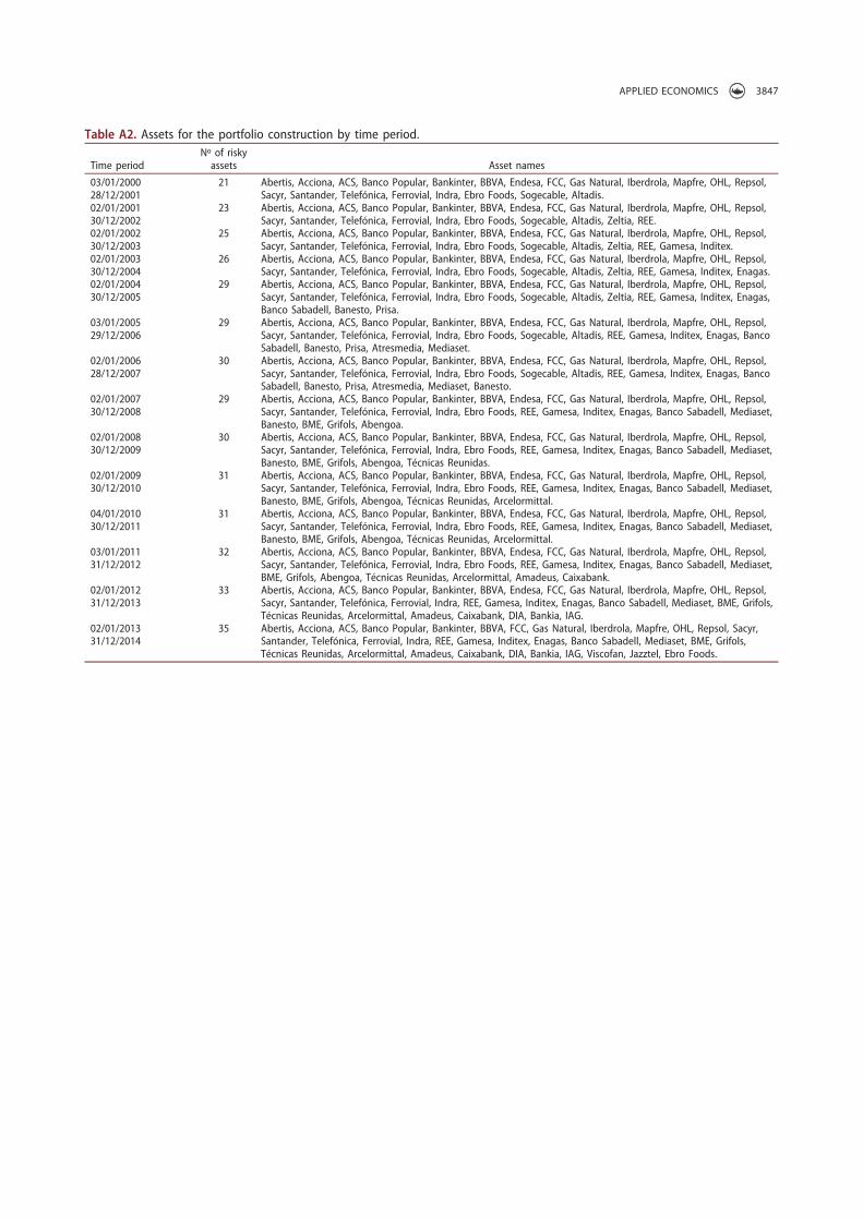
Table A2. Assets for the portfolio construction by time period.
Time periodNº of riskyassets Asset names
03/01/200028/12/2001
21 Abertis, Acciona, ACS, Banco Popular, Bankinter, BBVA, Endesa, FCC, Gas Natural, Iberdrola, Mapfre, OHL, Repsol,Sacyr, Santander, Telefónica, Ferrovial, Indra, Ebro Foods, Sogecable, Altadis.
02/01/200130/12/2002
23 Abertis, Acciona, ACS, Banco Popular, Bankinter, BBVA, Endesa, FCC, Gas Natural, Iberdrola, Mapfre, OHL, Repsol,Sacyr, Santander, Telefónica, Ferrovial, Indra, Ebro Foods, Sogecable, Altadis, Zeltia, REE.
02/01/200230/12/2003
25 Abertis, Acciona, ACS, Banco Popular, Bankinter, BBVA, Endesa, FCC, Gas Natural, Iberdrola, Mapfre, OHL, Repsol,Sacyr, Santander, Telefónica, Ferrovial, Indra, Ebro Foods, Sogecable, Altadis, Zeltia, REE, Gamesa, Inditex.
02/01/200330/12/2004
26 Abertis, Acciona, ACS, Banco Popular, Bankinter, BBVA, Endesa, FCC, Gas Natural, Iberdrola, Mapfre, OHL, Repsol,Sacyr, Santander, Telefónica, Ferrovial, Indra, Ebro Foods, Sogecable, Altadis, Zeltia, REE, Gamesa, Inditex, Enagas.
02/01/200430/12/2005
29 Abertis, Acciona, ACS, Banco Popular, Bankinter, BBVA, Endesa, FCC, Gas Natural, Iberdrola, Mapfre, OHL, Repsol,Sacyr, Santander, Telefónica, Ferrovial, Indra, Ebro Foods, Sogecable, Altadis, Zeltia, REE, Gamesa, Inditex, Enagas,Banco Sabadell, Banesto, Prisa.
03/01/200529/12/2006
29 Abertis, Acciona, ACS, Banco Popular, Bankinter, BBVA, Endesa, FCC, Gas Natural, Iberdrola, Mapfre, OHL, Repsol,Sacyr, Santander, Telefónica, Ferrovial, Indra, Ebro Foods, Sogecable, Altadis, REE, Gamesa, Inditex, Enagas, BancoSabadell, Banesto, Prisa, Atresmedia, Mediaset.
02/01/200628/12/2007
30 Abertis, Acciona, ACS, Banco Popular, Bankinter, BBVA, Endesa, FCC, Gas Natural, Iberdrola, Mapfre, OHL, Repsol,Sacyr, Santander, Telefónica, Ferrovial, Indra, Ebro Foods, Sogecable, Altadis, REE, Gamesa, Inditex, Enagas, BancoSabadell, Banesto, Prisa, Atresmedia, Mediaset, Banesto.
02/01/200730/12/2008
29 Abertis, Acciona, ACS, Banco Popular, Bankinter, BBVA, Endesa, FCC, Gas Natural, Iberdrola, Mapfre, OHL, Repsol,Sacyr, Santander, Telefónica, Ferrovial, Indra, Ebro Foods, REE, Gamesa, Inditex, Enagas, Banco Sabadell, Mediaset,Banesto, BME, Grifols, Abengoa.
02/01/200830/12/2009
30 Abertis, Acciona, ACS, Banco Popular, Bankinter, BBVA, Endesa, FCC, Gas Natural, Iberdrola, Mapfre, OHL, Repsol,Sacyr, Santander, Telefónica, Ferrovial, Indra, Ebro Foods, REE, Gamesa, Inditex, Enagas, Banco Sabadell, Mediaset,Banesto, BME, Grifols, Abengoa, Técnicas Reunidas.
02/01/200930/12/2010
31 Abertis, Acciona, ACS, Banco Popular, Bankinter, BBVA, Endesa, FCC, Gas Natural, Iberdrola, Mapfre, OHL, Repsol,Sacyr, Santander, Telefónica, Ferrovial, Indra, Ebro Foods, REE, Gamesa, Inditex, Enagas, Banco Sabadell, Mediaset,Banesto, BME, Grifols, Abengoa, Técnicas Reunidas, Arcelormittal.
04/01/201030/12/2011
31 Abertis, Acciona, ACS, Banco Popular, Bankinter, BBVA, Endesa, FCC, Gas Natural, Iberdrola, Mapfre, OHL, Repsol,Sacyr, Santander, Telefónica, Ferrovial, Indra, Ebro Foods, REE, Gamesa, Inditex, Enagas, Banco Sabadell, Mediaset,Banesto, BME, Grifols, Abengoa, Técnicas Reunidas, Arcelormittal.
03/01/201131/12/2012
32 Abertis, Acciona, ACS, Banco Popular, Bankinter, BBVA, Endesa, FCC, Gas Natural, Iberdrola, Mapfre, OHL, Repsol,Sacyr, Santander, Telefónica, Ferrovial, Indra, Ebro Foods, REE, Gamesa, Inditex, Enagas, Banco Sabadell, Mediaset,BME, Grifols, Abengoa, Técnicas Reunidas, Arcelormittal, Amadeus, Caixabank.
02/01/201231/12/2013
33 Abertis, Acciona, ACS, Banco Popular, Bankinter, BBVA, Endesa, FCC, Gas Natural, Iberdrola, Mapfre, OHL, Repsol,Sacyr, Santander, Telefónica, Ferrovial, Indra, REE, Gamesa, Inditex, Enagas, Banco Sabadell, Mediaset, BME, Grifols,Técnicas Reunidas, Arcelormittal, Amadeus, Caixabank, DIA, Bankia, IAG.
02/01/201331/12/2014
35 Abertis, Acciona, ACS, Banco Popular, Bankinter, BBVA, FCC, Gas Natural, Iberdrola, Mapfre, OHL, Repsol, Sacyr,Santander, Telefónica, Ferrovial, Indra, REE, Gamesa, Inditex, Enagas, Banco Sabadell, Mediaset, BME, Grifols,Técnicas Reunidas, Arcelormittal, Amadeus, Caixabank, DIA, Bankia, IAG, Viscofan, Jazztel, Ebro Foods.
APPLIED ECONOMICS 3847