portfolio selection with parameter and model uncertainty
TRANSCRIPT
Portfolio Selection with Parameter and Model Uncertainty:
A Multi-Prior Approach∗
Lorenzo Garlappi† Raman Uppal‡ Tan Wang§
April 2004
∗We gratefully acknowledge financial support from INQUIRE UK; this article however representsthe views of the authors and not of INQUIRE. We are very grateful to Lubos Pastor for extensivecomments. We thank Nicholas Barberis, Suleyman Basak, Ian Cooper, Victor DeMiguel, FranciscoGomes, Tim Johnson, Catalina Stefanescu, Yongjun Tang, Sheridan Titman, Roberto Wessels andparticipants at presentations given at Copenhagen Business School, Imperial College, LancasterUniversity, London Business School, University of Maryland, University of Texas at Austin, and theINQUIRE Fall 2003 conference for helpful suggestions.
†McCombs School of Business, The University of Texas at Austin, Austin TX, 78712; Email:[email protected].
‡London Business School and CEPR; IFA, 6 Sussex Place Regent’s Park, London, United King-dom NW1 4SA; Email: [email protected].
§University of British Columbia, 2053 Main Mall, Vancouver Canada V6T 1Z2, Canada; Email:[email protected].

Portfolio Selection with Parameter and Model Uncertainty:A Multi-Prior Approach
Abstract
In this paper, we extend the mean-variance portfolio model where expected returns are ob-tained using maximum likelihood estimation to explicitly account for uncertainty about theestimated expected returns. In contrast to the Bayesian approach to estimation error, wherethere is only a single prior and the investor is neutral to uncertainty, we allow for multiplepriors and aversion to uncertainty. We characterize the set of priors as a confidence intervalaround the estimated value of expected return and we model aversion to uncertainty via aminimization over the set of priors. The multi-prior model has several attractive features:One, just like the Bayesian model, the multi-prior model is firmly grounded in decisiontheory; Two, it is flexible enough to allow for uncertainty about expected returns estimatedjointly for all assets or different levels of uncertainty about expected returns for differentsubsets of the assets; Three, we show how in several special cases of the multi-prior modelone can obtain closed-form expressions for the optimal portfolio, which can be interpretedas a shrinkage of the mean-variance portfolio towards either the risk-free asset or the mini-mum variance portfolio. We illustrate how to implement the multi-prior model using bothinternational and domestic data. Our analysis suggests that allowing for parameter uncer-tainty reduces the fluctuation of portfolio weights over time and, for the data set considered,improves the out-of sample performance.
Keywords: Portfolio choice, asset allocation, estimation error, uncertainty, ambiguity, ro-bustness.JEL Classification: G11, D81
Contents
1 Introduction 1
2 Multi-prior approach to portfolio choice 52.1 The classical mean-variance portfolio model . . . . . . . . . . . . . . . . . . 62.2 Extension of the standard model to incorporate uncertainty aversion . . . . 7
2.2.1 Uncertainty about expected returns estimated asset-by-asset . . . . 82.2.2 Uncertainty about expected returns estimated jointly for all assets . 102.2.3 Uncertainty about expected returns estimated for subsets of assets . 112.2.4 Uncertainty about the return-generating model and expected returns 13
3 Comparison with other approaches to estimation error 153.1 A summary of the traditional Bayesian approach . . . . . . . . . . . . . . . 163.2 Comparison of the multi-prior approach with Bayesian approach . . . . . . 173.3 Analytic comparison of the portfolio weights from the various models . . . . 18
4 Empirical applications of the multi-prior approach 214.1 Uncertainty about expected returns: International data . . . . . . . . . . . 224.2 Uncertainty about expected returns and factor model: Domestic data . . . 26
5 Conclusion 28
A Appendix: Proofs of all propositions 30
List of Tables
1 Parameters for the two-asset one-factor example . . . . . . . . . . . . . . . 352 Portfolio weights for the two-asset one-factor example . . . . . . . . . . . . 363 Summary statistics for international data . . . . . . . . . . . . . . . . . . . 374 Out-of-sample performance of various portfolios using international data . 385 Out-of-sample Sharpe Ratios for various portfolios using domestic data with
ω = 0 . . . . . . . . . . . . . . . . . . . . . . . . . . . . . . . . . . . . . . . 396 Out-of-sample Sharpe Ratios for various portfolios using domestic data with
ω = 1 . . . . . . . . . . . . . . . . . . . . . . . . . . . . . . . . . . . . . . . 40
List of Figures
1 Portfolio weights in the US index over time . . . . . . . . . . . . . . . . . . 412 Shrinkage factors φMP (ε) and φBS over time . . . . . . . . . . . . . . . . . 423 Portfolio weights assuming expected returns estimated using MLE . . . . . 434 Portfolio weights assuming factor model (CAPM) for expected returns . . 45

1 Introduction
Expected returns, variances, and covariances are estimated with error. But classical mean-
variance portfolio optimization ignores the estimation error, and consequently, the mean-
variance portfolio formed using sample moments has extreme portfolio weights that fluctuate
substantially over time and the out-of-sample performance of such a portfolio is quite poor.1
The standard decision-theoretic approach2 adopted in the literature to deal with estimation
error is to use Bayesian “shrinkage” estimators that incorporate a prior.3 But, the Bayesian
approach assumes that the decision-maker has only a single prior or is neutral to uncertainty
in the sense of Knight (1921).
Given the difficulty in estimating moments of asset returns, it is much more likely that
investors have multiple priors rather than a single prior about moments of asset returns.
Moreover, there is substantial evidence from economic experiments that agents are not neu-
tral to the ambiguity arising from having multiple priors (Ellsberg (1961)), with the aversion
to uncertainty being particularly strong in cases where people feel that their competence in
assessing the relevant probabilities is low (Heath and Tversky (1991)) and when subjects
are told that there may be other people who are more qualified to evaluate a particular risky
position (Fox and Tversky (1995)). A recent literature, for instance, Anderson, Hansen, and
Sargent (1999), Chen and Epstein (2002), and Uppal and Wang (2003), develops models of
decision making that allow for multiple priors and where the decision maker is not neutral to
uncertainty. Our objective in this paper is to examine the implications of these theoretical
models for investment management.1For a discussion of the problems entailed in implementing mean-variance optimal portfolios, see Hodges
and Brealey (1978), Michaud (1989), Best and Grauer (1991), and Litterman (2003).2Other approaches for dealing with estimation error are to impose arbitrary portfolio constraints prohibit-
ing shortsales (Frost and Savarino (1988) and Chopra (1993)), which Jagannathan and Ma (2003) show canbe interpreted as shrinking the extreme elements of the covariance matrix, and the use of resampling basedon simulations advocated by Michaud (1998). Scherer (2002) describes the resampling approach in detail anddiscusses some of its limitations, while Harvey, Liechty, Liechty, and Muller (2003) discuss other limitationsand provide an estimate of the loss incurred by an investor who chooses a portfolio based on this approach.Black and Litterman (1990, 1992) propose an approach that combines two sets of priors—one based on anequilibrium asset pricing model and the other based on the subjective views of the investor—which is notstrictly Bayesian because a Bayesian approach combines a prior with the data.
3In the literature, the Bayesian adjustment has been implemented in different ways. Barry (1974),and Bawa, Brown, and Klein (1979), use either a non-informative diffuse prior or a predictive distributionobtained by integrating over the unknown parameter. In a second implementation, Jobson and Korkie(1980), Jorion (1985, 1986), Frost and Savarino (1986), and Dumas and Jacquillat (1990), use empiricalBayes estimators, which shrinks estimated returns closer to a common value and moves the portfolio weightscloser to the global minimum-variance portfolio. In a third implementation, Pastor (2000), and Pastor andStambaugh (2000) use the equilibrium implications of an asset pricing model to establish a prior; thus, inthe case where one uses the CAPM to establish the prior, the resulting weights move closer to those for avalue-weighted portfolio.
Portfolio selection with parameter and model uncertainty 2
Our main contribution is to show how the multi-prior model of decision making can be
applied to the practical problem of portfolio selection when expected returns are estimated
with error,4 and to compare explicitly the portfolio weights from this approach with those
from the mean-variance and traditional Bayesian models. We demonstrate how to formulate
the portfolio selection problem of an uncertainty-averse fund manager. This formulation
relies on two changes to the standard mean-variance model: (i) We impose an additional
constraint on the mean-variance portfolio optimization program that restricts the expected
return for each asset to lie within a specified confidence interval of its estimated value; and
(ii) We permit the fund manager to minimize over the choice of expected returns and/or
models subject to this constraint, in addition to the standard maximization over portfolio
weights. The additional constraint recognizes the possibility of estimation error; that is, the
point estimate of the expected return is not the only possible value of the expected return
considered by the investor. The minimization over the estimated expected returns reflects
the investor’s aversion to uncertainty; that is, in contrast to the standard mean-variance
model or the Bayesian approach, in the model we consider the investor is not neutral toward
uncertainty.5
To understand the intuition underlying the multi-prior model, observe that because of
the constrained minimization over expected returns, when the confidence interval is large
for a particular risky asset (that is, the mean is estimated imprecisely), then the investor
relies less on the estimated mean, and hence, reduces the weight invested in this asset.
When this interval is small, the minimization is constrained more tightly, and hence, the
portfolio weight is closer to the standard weight that one would get from a model that
ignores estimation error. In the limit, when the confidence interval is zero, the optimal
weights are those from the classical mean-variance model.
Our formulation of the multi-prior model of portfolio selection has several attractive
features. One, just like the Bayesian model, the multi-prior model is firmly grounded in
decision theory—the max-min characterization of the objective function is consistent with4We focus on the error in estimating expected returns of assets because as shown in Merton (1980) they
are much harder to estimate than the variances and covariances. Moreover, Chopra and Ziemba (1993)estimate the cash-equivalent loss from the use of estimated rather than true parameters. They find thaterrors in estimating expected returns are over ten times as costly as errors in estimating variances, and overtwenty times as costly as errors in estimating covariances. For a discussion of the problems in estimatingthe covariance matrix in the context of portfolio optimization, see Best and Grauer (1992), Ledoit (1996),Chan, Karceski, and Lakonishok (1999), and Ledoit and Wolf (2003).
5See Section 2 and Bewley (1988) for a discussion of how confidence intervals obtained from classicalstatistics are related to Knightian uncertainty and Bayesian models of decision making.
Portfolio selection with parameter and model uncertainty 3
the multi-prior approach advocated by Gilboa and Schmeidler (1989) and developed in
a static setting by Dow and Werlang (1992) and Kogan and Wang (2002), in dynamic
discrete-time by Epstein and Wang (1994), and in continuous time by Chen and Epstein
(2002). Two, in several economically interesting cases, we show that the multi-prior model
can be simplified to a mean-variance model but where the expected return is adjusted to
reflect the investor’s uncertainty about its estimate. The analytic expressions we obtain for
the optimal portfolio weights allow us to provide insights about the effects of parameter
and model uncertainty in a multi-prior setting. For instance, in one special case where we
obtain a closed-form solution, we show that the optimal portfolio weights can be interpreted
as a weighted average of the classical mean-variance portfolio and the minimum-variance
portfolio, with the weights depending on the precision with which expected returns are
estimated and the investor’s aversion to uncertainty. This special case is of particular
importance because it allows us to compare the multi-prior approach of this paper with the
traditional Bayesian approach in the literature. The analytic solutions also indicate how
the multi-prior model can be implemented as a simple maximization problem instead of a
much more complicated saddle point problem.
Three, the multi-prior model is flexible enough to allow for the case where the expected
returns on all assets are estimated jointly and also where the expected returns on assets
are estimated in subsets. The estimation may be undertaken using classical methods such
as maximum likelihood or using a Bayesian approach. Moreover, the framework can incor-
porate both parameter and model uncertainty; that is, it can be implemented when one is
estimating expected returns from their sample moments or when one is using a particular
factor model for returns such as APT or the CAPM and there is uncertainty about this
being the true model. Four, the multi-prior model does not introduce ad-hoc short-sale
constraints on portfolio weights that rule out short positions even if these were optimal
under the true parameter values. Instead, the constraints imposed in the multi-prior model
arise because of the investor’s aversion to parameter and model uncertainty. At the same
time, our formulation of the multi-prior model can accommodate real-world constraints on
the size of trades or position limits.6 Finally, in contrast to the Bayesian approach where6In addition to the features described above, the multi-prior approach is consistent with any utility
function, not just utility defined over mean and variance—our focus on the mean-variance objective functionis only because of our desire to compare our results to those in this literature.
Portfolio selection with parameter and model uncertainty 4
the investor is neutral to uncertainty, the multi-prior model captures the investor’s aversion
to uncertainty about both estimated parameters and the return-generating model.
Our paper is closely related to several papers in the literature. Goldfarb and Iyengar
(2003), Halldorsson and Tutuncu (2000), and Tutuncu and Koenig (2003) develop algo-
rithms for solving max-min saddle-point problems numerically and apply the algorithms
to portfolio choice problem, while Wang (2003) shows how to obtain the optimal portfolio
numerically in a Bayesian setting in the presence of uncertainty. Our paper differs from
Goldfarb and Iyengar (2003), Halldorsson and Tutuncu (2000), and Tutuncu and Koenig
(2003) in serval respects. First, we incorporate not only parameter uncertainty, but also
model uncertainty. Second, we introduce joint constraints on expected returns instead of
only individual constraints as in Goldfarb and Iyengar (2003), Halldorsson and Tutuncu
(2000), and Tutuncu and Koenig (2003). Finally, as mentioned above, for several special
cases we obtain not just numerical solutions but also closed-form expressions for the optimal
portfolio weights, which enables us to provide an economic interpretation of the effect of
aversion to uncertainty.
In order to understand the difference between the properties of the portfolio weights
from the multi-prior approach and the mean-variance and Bayesian models, we apply the
multi-prior model to two portfolio selection problems. In the first application, we consider
the problem of a fund manager allocating wealth across eight international equity indices
and who is uncertain about the expected returns on these equity indices. In the second
application, we consider the problem of a fund manager who is uncertain about the expected
returns on two investable portfolios, HML and SMB, and also about the market-model
generating returns on these portfolios. For both applications, we characterize the properties
of the portfolio weights under the multi-prior approach and compare them to the standard
mean-variance portfolio that ignores estimation error and the Bayesian portfolio that allows
for estimation error but has a single prior or is uncertainty neutral. Even though the utility
function under which each of these portfolios is selected is not the same, we report the
out-of-sample performance of these portfolios so that prospective users of the model can
evaluate the various models.
For the international data set, we find that the portfolio weights using the multi-prior
model are less unbalanced and vary much less over time compared to the mean-variance

Portfolio selection with parameter and model uncertainty 5
portfolio weights. More importantly, the out-of-sample returns generated by the multi-
prior portfolio model have a substantially higher mean and lower volatility compared to the
standard mean-variance portfolio strategy. The portfolio that incorporate aversion to un-
certainty also outperforms the Bayes-diffuse-prior and the empirical Bayes-Stein portfolios.
The explanation for this is that the uncertainty averse portfolio and the Bayesian portfolios
consist of a weighted average of the mean-variance and minimum-variance portfolios, the
uncertainty averse portfolio puts a higher weight on the minimum-variance portfolio, and
in this data set the expected returns are so noisy that it is optimal to ignore estimates
of expected returns all together. The second application considers the case where returns
are assumed to be driven by a single-factor (CAPM) model, and the fund manager faces
both parameter and model uncertainty when deciding how to allocate wealth to the Fama-
French HML and SMB portfolios and the market portfolio. In this case, we find that the
portfolio has a substantial proportion of wealth in the riskfree asset—typically more than
the Bayesian model would suggest. Moreover, when the multi-prior portfolio allows for
a small degree of uncertainty its out-of-sample Sharpe Ratio is greater than that of the
mean-variance portfolio and the Bayesian portfolios.
The rest of the paper is organized as follows. In Section 2, we show how one can
formulation the problem of portfolio selection for a fund manager who is averse to parameter
and model uncertainty and illustrate this formulation through a simple example with only
two risky assets. In Section 3, we discuss the relation of the multi-prior model to the
traditional Bayesian approach for dealing with estimation error and we compare analytically
the portfolio weights under the two approaches. Then, in Section 4, we illustrate the out-of-
sample properties of the multi-prior model by considering two empirical portfolio selection
settings: in the first, the investor has to allocate wealth across eight international equity-
market indices, and in the second the investor has to allocate wealth to the market portfolio
and two Fama-French portfolios, HML and SMB. Our conclusions are presented in Section 5.
Proofs for propositions are collected in the Appendix.
2 Multi-prior approach to portfolio choice
This section is divided into two parts. In the first, Section 2.1, we summarize the standard
mean-variance model of portfolio choice where estimation error is ignored. In the second

Portfolio selection with parameter and model uncertainty 6
part, Section 2.2, we show how this model can be extended to incorporate aversion to
uncertainty about the estimated parameters and the return-generating model.
2.1 The classical mean-variance portfolio model
According to the classical mean-variance model (Markowitz (1952, 1959), Sharpe (1970)),
the optimal portfolio of N risky assets, w, is given by the solution of the following opti-
mization problem,
maxw
w>µ− γ
2w>Σw, (1)
where µ is the N -vector of the true expected excess returns, Σ is the N × N covariance
matrix, 1N is a N -vector of ones and the scalar γ is the risk aversion parameter. The
solution to this problem is
w =1γ
Σ−1µ, (2)
In the absence of a risk-free asset, the problem faced by the investor has the same form
as (1) with the difference that µ represents the vector of true expected return and the
portfolio weights has to sum to one. The solution in this case is
w =1γ
Σ−1(µ− µ0 1N
), (3)
where µ0 is the expected return on the zero-beta portfolio associated with the optimal
portfolio w and is given by
µ0 =B − γ
A, (4)
where A = 1>NΣ−11N and B = µ>Σ−11N .
A fundamental assumption of the standard mean-variance portfolio selection model
in (1) is that the investor knows the true expected returns. In practice, however, the
investor has to estimate expected returns. Denoting the estimate of expected returns by µ,
the actual problem that the investor solves is
maxw
w>µ− γ
2w>Σw. (5)
subject to w>1N = 1. The problem in (5) coincides with (1) only if expected returns are
estimated with infinite precision, that is, µ = µ. In reality, however, expected returns are
Portfolio selection with parameter and model uncertainty 7
notoriously difficult to estimate. As a result, portfolio weights obtained from solving (5) tend
to consist of extreme positions that swing dramatically over time. Moreover, these optimal
portfolios often perform poorly out of sample even compared to portfolios selected according
to some simple ad hoc rules, such as holding the value-weighted or equally-weighted market
portfolio.
2.2 Extension of the standard model to incorporate uncertainty aversion
To explicitly take into account that asset expected returns are estimated imprecisely, we
introduce two new components into the standard mean-variance portfolio selection problem
in (1). One, we impose an additional constraint on the mean-variance optimization program
that restricts the expected return for each asset to lie within a specified confidence interval
of its estimated value. This constraint implies that the investor recognizes explicitly the
possibility of estimation error; that is, the point estimate of the expected return is not the
only possible value considered by the investor. Two, we introduce an additional optimiza-
tion—the investor is allowed to minimize over the choice of expected returns and/or models
subject to the additional constraint. This minimization over expected returns, µ, reflects
the investor’s aversion to uncertainty (Gilboa and Schmeidler (1989)).
With the two changes to the standard mean-variance model described above, the multi-
prior model takes the following form in general:
maxw
minµ
w>µ− γ
2w>Σw, (6)
subject to
f(µ, µ,Σ) ≤ ε, (7)
w>1N = 1, (8)
where f(·) is a vector-valued function, and ε is a vector of constants that reflects both the
investor’s uncertainty and his aversion to uncertainty. The role of ε will be explained further
below. As before, equation (8) constrains the weights to sum to unity in the absence of a
riskfree asset; when a riskfree asset is available, this constraint can be dropped.
In the rest of this section we illustrate several possible specifications of the constraint
given in (7) and their implications for portfolio selection.
Portfolio selection with parameter and model uncertainty 8
2.2.1 Uncertainty about expected returns estimated asset-by-asset
We start by considering the case where f(µ, µ,Σ) has N components,
fj(µ, µ,Σ) =(µj − µj)2
σ2j /Tj
, j = 1, . . . , N, (9)
where Tj is the number of observations in the sample for asset j. In this case, the constraint
in (7) becomes
(µj − µj)2
σ2j /Tj
≤ εj , j = 1, . . . , N. (10)
The constraints (10) have an immediate interpretation as confidence intervals. For
instance, it is well known that if returns are assumed to be normally distributed then µj−µj
σj/√
Tj
follows a normal distribution.7 Thus, the εj in constraints (10) determines a confidence
interval. When all the N constraints in (10) are taken together, (10) is closely related to
the probabilistic statement
P (µ1 ∈ I1, . . . , µN ∈ IN ) = 1− p, (11)
where Ij , j = 1, . . . , N , are intervals in the real line. Here p is a significance level. For
instance, if the returns are independent of each other and if pj is the significance level
associated with εj , then the probability that all the N true expected returns fall into the
N intervals, respectively, is 1− p = (1− p1)(1− p2) · · · (1− pN ).8
While confidence intervals or significance levels are often associated with hypothesis
testing in statistics, Bewley (1988) shows that they can be interpreted as a measure of the
level of uncertainty associated with the parameters estimated. An intuitive way to see it is
to envision an econometrician who estimates the expected returns for an investor. He can
report to the investor his best estimates of the expected returns. He can at the same time
report the uncertainty of his estimates by stating, say, the confidence level of µj ∈ Ij for all
j = 1, . . . , j = N , is 95%.7If σj is unknown then it follows a t-distribution with Tj − 1 degrees of freedom.8When the asset returns are not independent, the calculation of the confidence level of the event involves
multiple integrals. In general, it is difficult to obtain a closed-form expression for the confidence level. Thefact that the data for different assets may be of different lengths does not present a serious problem for themultivariate normal distribution setting as shown by Stambaugh (1997).
Portfolio selection with parameter and model uncertainty 9
When viewed in isolation, (10) can have the simple interpretation as measure of un-
certainty just described. When it is combined with the maxmin problem (6), i.e., when it
is used in an investor’s portfolio selection problem, however, it also captures the investor’s
aversion to uncertainty. For example, suppose that the standard practice of econometricians
is to report 95% confidence interval. If the investor has high uncertainty aversion, he could
use an ε that corresponds to a 99% confidence interval. In other words, by picking the
appropriate εj the investor can indicate the level of uncertainty he has about the estimate
of the expected return of asset j as well as his level of uncertainty aversion.
To gain some intuition regarding the effect of uncertainty about the estimated mean on
the optimal portfolio weight, one can simplify the max-min portfolio problem, subject to
the constraint in (10), as follows.
Proposition 1 The max-min problem (6) subject to (8) and (10) is equivalent to the fol-
lowing maximization problem
maxw
w>(µ− µadj)− γ
2w>Σw
, (12)
subject to (8), where µadj is the N -vector of adjustments to be made to the estimated expected
return:
µadj ≡sign(w1)
σ1√T
√ε1, . . . , sign(wN )
σN√T
√εN
. (13)
The proposition above shows that the multi-prior model, which is expressed in terms of
a max-min optimization, can be interpreted as the mean-variance optimization problem in
(5), but where the mean has been adjusted to reflect the uncertainty about its estimated
value. The term sign(wj) in (13) ensures that the adjustment leads to a shrinkage of the
portfolio weights; that is, if a particular portfolio weight is positive (long position) then the
expected return on this asset is reduced, while if it is negative (short position) the expected
return on the asset is increased. In Section 2.2.3, we characterize the optimal solution for
this problem.
Portfolio selection with parameter and model uncertainty 10
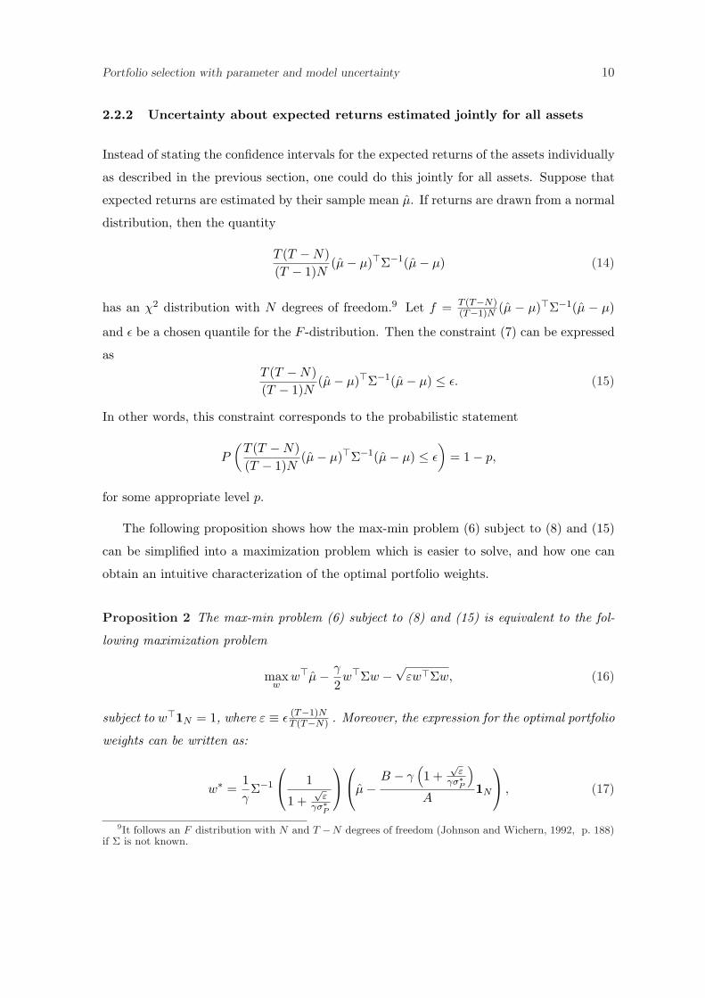
2.2.2 Uncertainty about expected returns estimated jointly for all assets
Instead of stating the confidence intervals for the expected returns of the assets individually
as described in the previous section, one could do this jointly for all assets. Suppose that
expected returns are estimated by their sample mean µ. If returns are drawn from a normal
distribution, then the quantity
T (T −N)(T − 1)N
(µ− µ)>Σ−1(µ− µ) (14)
has an χ2 distribution with N degrees of freedom.9 Let f = T (T−N)(T−1)N (µ − µ)>Σ−1(µ − µ)
and ε be a chosen quantile for the F -distribution. Then the constraint (7) can be expressed
asT (T −N)(T − 1)N
(µ− µ)>Σ−1(µ− µ) ≤ ε. (15)
In other words, this constraint corresponds to the probabilistic statement
P
(T (T −N)(T − 1)N
(µ− µ)>Σ−1(µ− µ) ≤ ε
)= 1− p,
for some appropriate level p.
The following proposition shows how the max-min problem (6) subject to (8) and (15)
can be simplified into a maximization problem which is easier to solve, and how one can
obtain an intuitive characterization of the optimal portfolio weights.
Proposition 2 The max-min problem (6) subject to (8) and (15) is equivalent to the fol-
lowing maximization problem
maxw
w>µ− γ
2w>Σw −
√εw>Σw, (16)
subject to w>1N = 1, where ε ≡ ε (T−1)NT (T−N) . Moreover, the expression for the optimal portfolio
weights can be written as:
w∗ =1γ
Σ−1
1
1 +√
εγσ∗P
µ−
B − γ(1 +
√ε
γσ∗P
)
A1N
, (17)
9It follows an F distribution with N and T −N degrees of freedom (Johnson and Wichern, 1992, p. 188)if Σ is not known.

Portfolio selection with parameter and model uncertainty 11
where A = 1>N Σ−1 1N , B = µ>Σ−1 1N , and σ∗P is the variance of the optimal portfolio that
can be obtained from solving the polynomial equation (A11) in Appendix A.
We can now use the expression in (17) for the optimal weights to interpret the effect of
parameter uncertainty. Note that as ε → 0, that is either ε → 0 or T → ∞, the optimal
weight w∗ converges to the mean-variance portfolio10
w∗ =1γ
Σ−1(
µ− B − γ
A1N
)
=1γ
Σ−1(µ− µ01N
), (18)
where B−γA = µ0 is the expected return on the zero-beta portfolio associated with w∗ defined
in equation (3). Thus, in the absence of parameter uncertainty the optimal portfolio reduces
to the mean-variance weights. On the other hand, as ε →∞ the optimal portfolio converges
to
w∗ =1A
Σ−11N , (19)
which is the minimum-variance portfolio. These results suggest that parameter uncertainty
shifts the optimal portfolio away from the mean-variance weights toward the minimum-
variance weights.
2.2.3 Uncertainty about expected returns estimated for subsets of assets
In Section 2.2.1 we described the case where there was uncertainty about expected returns
that were estimated individually asset-by-asset, and in Section 2.2.2 we described the case
where the expected returns were estimated jointly for all assets. Stambaugh (1997) provides
motivation for why one may wish to do this – for example, the lengths of available histories
may differ across the assets being considered. In this section, we present a generalization
that allows the estimation to be done separately for different subclasses of assets, and we
show that this generalization unifies the two specifications described above.10In taking these limits, it is important to realize that σ∗P also depends on the weights. In order to obtain
the correct limits, it is useful to look at equation (A11), which characterizes σ∗P .
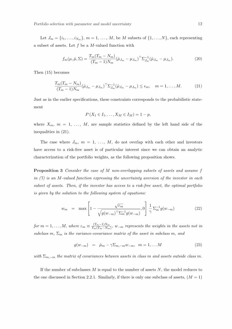
Portfolio selection with parameter and model uncertainty 12
Let Jm = i1, . . . , iNm, m = 1, . . . , M , be M subsets of 1, . . . , N, each representing
a subset of assets. Let f be a M -valued function with
fm(µ, µ,Σ) =Tm(Tm −Nm)(Tm − 1)Nm
(µJm − µJm)>Σ−1Jm
(µJm − µJm). (20)
Then (15) becomes
Tm(Tm −Nm)(Tm − 1)Nm
(µJm − µJm)>Σ−1Jm
(µJm − µJm) ≤ εm, m = 1, . . . , M. (21)
Just as in the earlier specifications, these constraints corresponds to the probabilistic state-
ment
P (X1 ∈ I1, . . . , XM ∈ IM ) = 1− p,
where Xm, m = 1, . . . , M , are sample statistics defined by the left hand side of the
inequalities in (21).
The case where Jm, m = 1, . . . , M , do not overlap with each other and investors
have access to a risk-free asset is of particular interest since we can obtain an analytic
characterization of the portfolio weights, as the following proposition shows.
Proposition 3 Consider the case of M non-overlapping subsets of assets and assume f
in (7) is an M -valued function expressing the uncertainty aversion of the investor in each
subset of assets. Then, if the investor has access to a risk-free asset, the optimal portfolio
is given by the solution to the following system of equations:
wm = max
1−
√εm√
g(w−m)>Σ−1m g(w−m)
, 0
1
γΣ−1
m g(w−m) (22)
for m = 1, . . . ,M, where εm ≡ (Tm−1)Nm
Tm(Tm−Nm) , w−m represents the weights in the assets not in
subclass m, Σm is the variance-covariance matrix of the asset in subclass m, and
g(w−m) = µm − γΣm,−mw−m, m = 1, . . . M (23)
with Σm,−m the matrix of covariances between assets in class m and assets outside class m.
If the number of subclasses M is equal to the number of assets N , the model reduces to
the one discussed in Section 2.2.1. Similarly, if there is only one subclass of assets, (M = 1)

Portfolio selection with parameter and model uncertainty 13
the model reduces to the one studied in Section 2.2.2. The following two corollaries formalize
this relation and characterize the optimal portfolios.
Corollary 1 If the number of subclasses M is equal to the number of assets N and there
is a risk-free asset, the optimal portfolio in problem (6) is given by solving the following
system of simultaneous equations
wi = max [ |g(w−i)| − √εi, 0 ]1
γσisign[g(w−i)], i = 1, 2, . . . , N (24)
where εi = εiT , w−i are the N − 1 portfolio weights on the assets other than i,
g(w−i) = µi − Σi,−iw−i
and Σi,−i is the i-th row of the variance-covariance matrix with the i-th element removed.
Corollary 2 If there is only one subclass of assets, that is M = 1, then in the presence of
a risk-free asset, the optimal portfolio is given by
w = max
[1−
√ε
µ>Σ−1µ, 0
]1γ
Σ−1µ, where ε ≡ ε(T − 1)NT (T −N)
. (25)
2.2.4 Uncertainty about the return-generating model and expected returns
In this section, we explain how the general model developed in Section 2.2.3 where there are
M subsets of assets can be used to analyze situations where investors rely on a factor model
to generate estimates of expected return and are averse to both the estimated expected
returns on the factor portfolios and the model used to generate the expected returns on
investable assets.
To illustrate this situation, consider the case of a market with N risky asset in which
an asset pricing model with K factors is given. Denote with rat the N × 1 vector of excess
returns of the non-benchmark assets over the risk-free rate in period t. Similarly, denote by
rft the excess return over the benchmark assets. The mean and variance of the assets and
factors are:
µ =
(µa
µf
), Σ =
(Σaa Σaf
Σfa Σff
). (26)

Portfolio selection with parameter and model uncertainty 14
We can always summarize the mean and variance of the assets by the parameters of the
following regression model
rat = α + βrft + ut, cov(ut, u>t ) = Ω, (27)
where α is a N × 1 vector, β is a N ×K matrix of factor loadings, and ut is a N × 1 vectors
of residuals with covariance Ω. Hence, the mean and variance of the returns can always be
expressed as follows
µ =
(α + βµf
µf
), Σ =
(βΣffβ> + Ω βΣff
Σffβ> Σff
). (28)
An investor who is averse to uncertainty about both the expected returns on the factors
and the model generating the returns on the assets will solve the following problem. Defining
w ≡ (wa, wf )> to be the (N + K)× 1 vector of portfolio weights, the investor’s problem is:
maxw
minµa,µf
w>µ− γ
2w>Σw, (29)
subject to
(µa − µa)>Σ−1aa (µa − µa) ≤ εa, (30)
(µf − µf )>Σ−1ff (µf − µf ) ≤ εf . (31)
Equations (30) and (31) capture parameter uncertainty over the estimate of the expected
returns. If investors use the asset pricing model to determine the estimate of µa, then
µa = βµf and equation (30) can be interpreted as a multi-prior characterization of model
uncertainty. Setting εa = 0 corresponds to imposing that the investor believes dogmatically
in the model.11
From Proposition 3 the solution to this problem is given by the following system of
equations
wa = max
1−
√εa√
g(wf )>Σ−1aa g(wf )
, 0
1
γΣ−1
aa g(wf ), (32)
wf = max
1−
√εf√
h(wa)>Σ−1ff h(wa)
, 0
1
γΣ−1
ff h(wa), (33)
11To be precise, the interpretation of equation (30) as a characterization of model uncertainty is true onlyif εf = 0. To see this, note that when µa = βµf , µa − µa = β(µf − µf )− α. Therefore, unless µf = µf thedifference µa − νa does not represent Jensen’s α.

Portfolio selection with parameter and model uncertainty 15
where
g(wf ) = µa − γΣafwf , (34)
h(wa) = µf − γΣfawa. (35)
To understand the structure of the solution to this problem we consider the case where
there are two assets and one factor. The parameters for these assets are summarized in
Table 1 and the optimal portfolio weights are reported in Table 2.12 Each panel corresponds
to a different level of uncertainty εf about the factor. Within each panel of the table, each
row represent a different level of uncertainty εa about the asset. A clear pattern emerges
from the portfolio weights reported in the table. First, when εf = 0 then for all values of
εa > 0 the investor is more uncertain about the assets than about the factor, and hence will
hold 100% of his wealth in the factor portfolio. Second, given a certain level of uncertainty
about the factor (i.e. keeping fixed εf > 0), as uncertainty in the asset estimate increases the
holdings of the risky non-benchmark assets decrease and the holding of the factor portfolio
increases. Third, given a certain level of uncertainty about the assets (i.e., keeping fixed
εa), as εf increases, the holdings of risky non-benchmark assets increase and the holding
of the factor decreases. These results are intuitive and suggest that the more uncertain is
the estimate of the expected return of an asset the less an investor is willing to invest in
that asset. Obviously, the uncertainty in the assets and the factors are interrelated and it is
ultimately the relative level of uncertainty between the two classes of asset that determines
the final portfolio.
3 Comparison with other approaches to estimation error
In this section, we relate the multi-prior framework for portfolio choice in the presence
of parameter and model uncertainty to other approaches considered in the literature, and
in particular, to portfolios that use the traditional Bayesian approach. We compare the
portfolio weights from the multi-prior model to the following: (i) the standard mean-variance
portfolio that ignores estimation error, (ii) the minimum-variance portfolio, (iii) the portfolio
based on Bayes-diffuse-prior estimates as in Bawa, Brown, and Klein (1979), and (iv) the12The parameters are chosen to match the results we would obtain by estimating a regression of the
monthly returns on the Fama-French portfolios HML and SMB on the Market from July 1926 to December2002. More details on this data set are provided in section 4.2.

Portfolio selection with parameter and model uncertainty 16
portfolio based on the empirical Bayes-Stein estimator, as described in Jorion (1985, 1986).
In this section, the comparison is done in terms of the theoretical foundations of the models
and their implications for portfolio weights, while in Section 4 this comparison is undertaken
empirically using two different data sets and the comparison set includes also the weights
obtained by using the data-and-model approach of Pastor (2000).
3.1 A summary of the traditional Bayesian approach
It is useful to begin with a brief summary of the traditional Bayesian approach. Let U(R) be
the utility function, where R is the return from the investment, and g(R|θ) the conditional
density (likelihood) of asset returns given parameter θ. In the setting of this paper, θ is
the vector of the expected returns of the risky assets. More generally, it can include the
covariances of the asset returns. If the parameter θ is known, then the conditional expected
utility of the investor is
E[U(R)|θ] =∫
U(R)g(R|θ)dR. (36)
In practice, however, the parameter θ is often unknown and needs to be estimated from
data, i.e., there is parameter uncertainty. In the presence of such parameter uncertainty,
Savage’s expected utility approach is to introduce a conditional prior (posterior) p(θ|X),
where X = (r1, . . . , rT ) is the vector of past returns, such that the expected utility is given
by
E[U(R)|X] = E [E[U(R)|θ]|X] =∫ ∫
U(R)g(R|θ)p(θ|X)dRdθ. (37)
Let π(θ) is the unconditional prior about the unknown parameter. Then the posterior
density given X is
p(θ|X) =∏T
t=1 g(rt|θ)π(θ)∫ ∏Tt=1 g(rt|θ)π(θ)dθ
, (38)
and the predictive density, given X, is
g(R|X) =∫
g(R|θ)p(θ|X)dθ =∫
g(R|θ)∏T
t=1 g(rt|θ)π(θ)∫ ∏Tt=1 g(rt|θ)π(θ)dθ
dθ. (39)
Using the predictive density, the expected utility of the investor is given by
E[U(R)|X] =∫
U(R)(∫
g(R|θ, X)p(θ|X)dθ
)dR =
∫U(R)g(R|X)dR. (40)

Portfolio selection with parameter and model uncertainty 17
Thus the key to the Bayesian approach is the incorporation of prior information and the
information from data in the calculation of the posterior and predictive distributions. The
effect of information on the investor’s decision comes through its effect on the predictive
distribution.
The foundation for the Bayesian approach was provided by Savage (1954). Early ap-
plications of this approach can be found in Klein and Bawa (1976), Jorion (1985, 1986).
More recent applications include Pastor (2000) and Pastor and Stambaugh (2000) who, in
addition to parameter uncertainty, consider also model uncertainty.
3.2 Comparison of the multi-prior approach with Bayesian approach
The decision-theoretic foundation of the multi-prior approach is laid by Gilboa and Schmei-
dler (1989). Equally well-founded axiomatically, the most important difference between
the Bayesian approach and the multi-prior approach is that in the Bayesian approach the
investor is implicitly assumed to be neutral to parameter and/or model uncertainty, while
in the multi-prior approach, the investor is averse to that uncertainty.
That in the Bayesian approach the investor is uncertainty neutral is best seen through
equation (40). The middle expression in the equation suggests that parameter and/or
model uncertainty enters the investor’s utility through the posterior p(θ|X), which can
affect the investor’s utility only through its effect on the predictive density g(R|X). In
other words, as far as the investor’s utility maximization decision is concerned, it does not
matter whether the overall uncertainty comes from the conditional distribution g(R|θ) of
the asset return or from the uncertainty about the parameter/model p(θ|X), as long as
the predictive distribution g(R|X) is the same. In other words, if the investor were in a
situation where there is no parameter/model uncertainty, say, because the past data X
could be used to identify the true parameter perfectly, and the distribution of asset returns
is characterized by g(R|X), then the investor would feel no different. In particular, there
is no meaningful separation of risk aversion and uncertainty aversion. In this sense, we say
that the investor is uncertainty neutral.
In the multi-prior framework, the risk (the conditional distribution g(R|θ) of the asset
returns is treated differently from the uncertainty about the parameter/model of the data
generating process. For example, in the portfolio choice problem described by equations
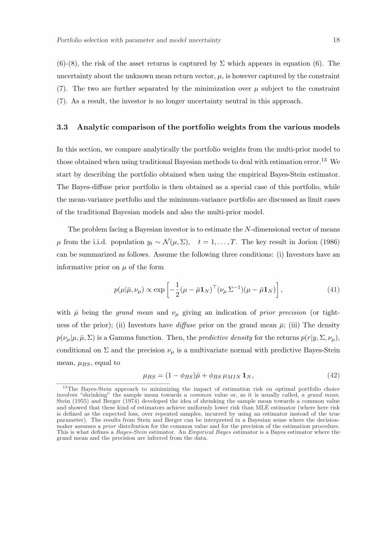
Portfolio selection with parameter and model uncertainty 18
(6)-(8), the risk of the asset returns is captured by Σ which appears in equation (6). The
uncertainty about the unknown mean return vector, µ, is however captured by the constraint
(7). The two are further separated by the minimization over µ subject to the constraint
(7). As a result, the investor is no longer uncertainty neutral in this approach.
3.3 Analytic comparison of the portfolio weights from the various models
In this section, we compare analytically the portfolio weights from the multi-prior model to
those obtained when using traditional Bayesian methods to deal with estimation error.13 We
start by describing the portfolio obtained when using the empirical Bayes-Stein estimator.
The Bayes-diffuse prior portfolio is then obtained as a special case of this portfolio, while
the mean-variance portfolio and the minimum-variance portfolio are discussed as limit cases
of the traditional Bayesian models and also the multi-prior model.
The problem facing a Bayesian investor is to estimate the N -dimensional vector of means
µ from the i.i.d. population yt ∼ N (µ,Σ), t = 1, . . . , T . The key result in Jorion (1986)
can be summarized as follows. Assume the following three conditions: (i) Investors have an
informative prior on µ of the form
p(µ|µ, νµ) ∝ exp[−1
2(µ− µ1N )>(νµ Σ−1)(µ− µ1N )
], (41)
with µ being the grand mean and νµ giving an indication of prior precision (or tight-
ness of the prior); (ii) Investors have diffuse prior on the grand mean µ; (iii) The density
p(νµ|µ, µ,Σ) is a Gamma function. Then, the predictive density for the returns p(r|y, Σ, νµ),
conditional on Σ and the precision νµ is a multivariate normal with predictive Bayes-Stein
mean, µBS , equal to
µBS = (1− φBS)µ + φBS µMIN 1N , (42)13The Bayes-Stein approach to minimizing the impact of estimation risk on optimal portfolio choice
involves “shrinking” the sample mean towards a common value or, as it is usually called, a grand mean.Stein (1955) and Berger (1974) developed the idea of shrinking the sample mean towards a common valueand showed that these kind of estimators achieve uniformly lower risk than MLE estimator (where here riskis defined as the expected loss, over repeated samples, incurred by using an estimator instead of the trueparameter). The results from Stein and Berger can be interpreted in a Bayesian sense where the decision-maker assumes a prior distribution for the common value and for the precision of the estimation procedure.This is what defines a Bayes-Stein estimator. An Empirical Bayes estimator is a Bayes estimator where thegrand mean and the precision are inferred from the data.
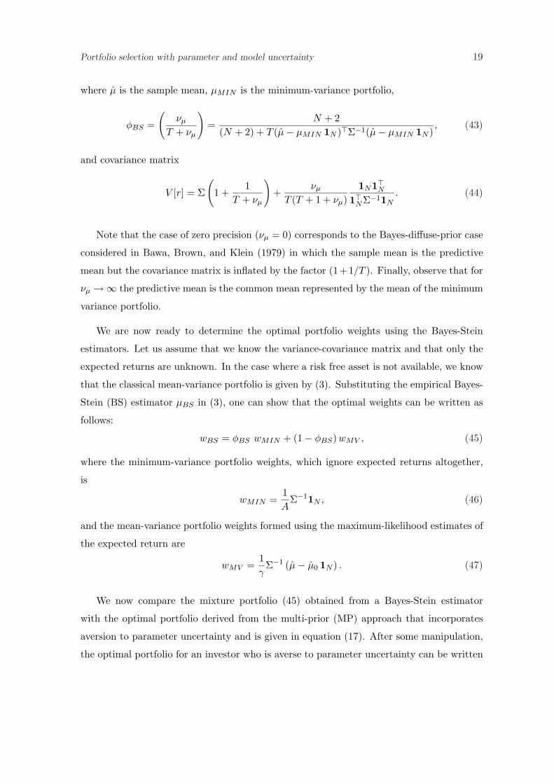
Portfolio selection with parameter and model uncertainty 19
where µ is the sample mean, µMIN is the minimum-variance portfolio,
φBS =
(νµ
T + νµ
)=
N + 2(N + 2) + T (µ− µMIN 1N )>Σ−1(µ− µMIN 1N )
, (43)
and covariance matrix
V [r] = Σ
(1 +
1T + νµ
)+
νµ
T (T + 1 + νµ)1N1>N
1>NΣ−11N. (44)
Note that the case of zero precision (νµ = 0) corresponds to the Bayes-diffuse-prior case
considered in Bawa, Brown, and Klein (1979) in which the sample mean is the predictive
mean but the covariance matrix is inflated by the factor (1+1/T ). Finally, observe that for
νµ →∞ the predictive mean is the common mean represented by the mean of the minimum
variance portfolio.
We are now ready to determine the optimal portfolio weights using the Bayes-Stein
estimators. Let us assume that we know the variance-covariance matrix and that only the
expected returns are unknown. In the case where a risk free asset is not available, we know
that the classical mean-variance portfolio is given by (3). Substituting the empirical Bayes-
Stein (BS) estimator µBS in (3), one can show that the optimal weights can be written as
follows:
wBS = φBS wMIN + (1− φBS) wMV , (45)
where the minimum-variance portfolio weights, which ignore expected returns altogether,
is
wMIN =1A
Σ−11N , (46)
and the mean-variance portfolio weights formed using the maximum-likelihood estimates of
the expected return are
wMV =1γ
Σ−1 (µ− µ0 1N ) . (47)
We now compare the mixture portfolio (45) obtained from a Bayes-Stein estimator
with the optimal portfolio derived from the multi-prior (MP) approach that incorporates
aversion to parameter uncertainty and is given in equation (17). After some manipulation,
the optimal portfolio for an investor who is averse to parameter uncertainty can be written
Portfolio selection with parameter and model uncertainty 20
as
wMP = φMP wMIN + (1− φMP ) wMV , (48)
where
φMP (ε) =
( √ε
γσ∗P +√
ε
)=
√ε (T−1)N
T (T−N)
γσ∗P +√
ε (T−1)NT (T−N)
, (49)
and wMIN and wMV are defined in (46) and (47), respectively.
Comparing the weights in equation (45) that are obtained using a Bayes-Stein estimator
to the weights in equation (48) obtained from the multi-prior model, we notice that both
methods shrink the mean-variance portfolio toward the minimum-variance portfolio, which
is the portfolio that essentially ignores all information about expected returns. However,
the magnitude of the shrinkage is different, that is, φBS 6= φMP (ε). In the next section,
where we implement these different portfolio strategies using real-world data, we will find
that the shrinkage factor from the multi-prior approach is much greater than that for the
empirical Bayes-Stein portfolio; that is, for reasonable values of ε, φMP (ε) > φBS .
So far, we have considered the following two cases: one, where the investor uses classical
maximum-likelihood estimators to estimate expected returns and then accounts for model
uncertainty in obtaining the weights in equation (48), and two, where the investor uses
Bayesian methods for estimating expected returns but ignores the possibility that these
estimates are uncertain, which leads to the portfolio weights in (45). But, one could just
as well have a third case where the estimation is done using Bayesian methods and the
investor allows for parameter uncertainty.14 In this case, the optimal portfolio weights are
given by the following expression.
wBSMP = φMP wMIN + (1− φMP ) wBS , (50)
where the minimum-variance-portfolio, wMIN , and the Bayesian portfolio, wBS , are defined
in (46) and (45), respectively. Observe that the expression in (50) is similar to that in (48)
but where wBS replaces wMV ; that is, the effect of uncertainty is to shrink the portfolio
that is now obtained using Bayesian estimation methods, wBS , toward wMIN . Notice that
in the limiting case where the investor is neutral toward uncertainty, setting ε = 0 in (50),14In this comparison, the Bayesian approach is interpreted narrowly as an estimation technique rather
than a decision-theoretic approach.

Portfolio selection with parameter and model uncertainty 21
which leads to φMP = 0, implies that the optimal portfolio reduces to wBS . This is the
sense in which the portfolio obtained using Bayesian estimation methods is nested in the
multi-prior approach.
One can also view the expression in (50) as being similar to that in (45), but where the
shrinkage factor consists not just of an adjustment because one is using Bayesian estimation
but also because the investor is averse to uncertainty. To see this, substitute in (50) the
expression for wBS in (45), to get
wBSMP = φBS
MP wMIN +(1− φBS
MP
)wML, (51)
where the shrinkage factor is now given by
φBSMP = φMP + φBS − φMP φBS . (52)
This expression again shows that if the investor is uncertainty neutral (ε = 0), then φMP = 0
and the optimal portfolio is the Bayesian portfolio wBS . If, on the other hand, there is zero
precision about the prior mean (νµ = 0), then φBS = 0 and the optimal portfolio is wMP .
And, only in the case where the investor is both uncertainty neutral and has zero precision
about the prior mean is it optimal to hold the standard mean-variance portfolio, wMV ,
which is obtained using maximum-likelihood estimates of the mean.
Of course, from equation (52) it is clear that φBSMP > φBS and φBS
MP > φMP , so the
investor who is using Bayesian estimation methods and is averse to uncertainty will shrink
his portfolio much more toward the minimum-variance portfolio, wMIN , than either the
investor who uses Bayesian estimation methods but is uncertainty averse, or the investor
who is uncertainty averse but has a diffuse prior so that he is using maximum-likelihood
estimates.
4 Empirical applications of the multi-prior approach
In this section, we show how to apply the multi-prior approach to portfolio selection. Our
goal in this section is (i) to demonstrate how the multi prior approach can be implemented
in practice and (ii) to compare the portfolio recommendations from this approach to other
procedures commonly used, with a particular emphasis on the Bayesian approach with
model uncertainty introduced in Pastor (2000).

Portfolio selection with parameter and model uncertainty 22
We consider two versions of the model. First, in Section 4.1 we illustrate the model
described in Section 2.2.2, where the expected returns on all assets are estimated jointly
and there is no riskfree asset. Then, in Section 4.2, we illustrate the model described in
Section 2.2.3 where there is both uncertainty about expected asset returns and the factor
model generating these returns and a riskfree asset is available. For the first application, we
use returns on eight international equity indices. For the second application, we consider
returns on a factor portfolio, which is the excess return on the US market portfolio (defined
as the value-weighted return on all NYSE, AMEX and NASDAQ stocks, minus the one-
month Treasury bill rate) and the Fama-French portfolios, HML and SMB. Details of these
two applications are given below.
4.1 Uncertainty about expected returns: International data
For our first empirical illustration we consider allocating wealth over eight international
equity indices whose returns are computed based on the month-end US-dollar value of the
equity index for the period January 1970 to July 2001. The equity indices are for Canada,
Japan, France, Germany, Italy, Switzerland, United Kingdom, United States. Data are
from MSCI (Morgan Stanley Capital International). The data set is similar to the one used
by De Santis and Gerard (1997) but spans for a longer time period than theirs. Summary
statistics for the indexes of the eight countries as well as for the MSCI world index are
provided in Table 3.
We assume that there is no risk-free asset and that the investor estimates the expected
returns jointly over portfolio by expressing uncertainty over the whole set of assets, as
described in Section 2.2.2. Using this model, we compute the mean-variance portfolios
that account for different degrees of uncertainty in the statistical estimate (ε) about the
expected returns. We also compute (i) the standard mean-variance portfolio that ignores
estimation error, (ii) the minimum-variance portfolio, and (iv) the portfolio based on Bayes-
Stein estimators, as described in Jorion (1985, 1986). From the result in Section 2.2.2 we
know that the resulting portfolio is a combination of the minimum variance portfolio and
the mean-variance portfolio.
To assess the performance of the different portfolio models, we determine the weights
from each model based on a window of 60 months and then calculate the return from holding
Portfolio selection with parameter and model uncertainty 23
this portfolio in the 61st month. We repeat this for the entire data set and compute the
average out-of sample means, volatilities and Sharpe ratios of each strategy. For each of the
portfolio models, we consider two cases: one, where short-selling is allowed, and the other
where short-selling is not allowed.
In our analysis, we set T = 60 because the estimation is done using a rolling-window of 60
months and we set N = 8 because there are eight country-indexes. Under the assumption
that the returns are normally distributed, if µ is taken to be the sample average of the
returns, the quantity T (T−N)(T−1)N (µ − µ)>Σ−1(µ − µ) is distributed as an F8,52. For reference
purpose, we recall that the 95-percentile of an F8,52 corresponds to ε = 2.122, while the
99-percentile corresponds to ε = 2.874.15
The results of our analysis are reported in Panel A of Table 4. Compared to the mean-
variance strategy in which historical mean returns µ are taken to be the estimator of ex-
pected returns µ, the portfolios constructed using the model that allows for parameter
uncertainty exhibit uniformly higher means and lower volatility.
Notice from Panel A that the case of ε = 0 corresponds to the mean-variance portfolio
while the case of ε →∞ corresponds to the minimum-variance portfolio, as discussed in the
previous section. Both the Bayes-diffuse-prior and the empirical Bayes-Stein portfolios show
lower mean and higher variance than any of the portfolios that account for uncertainty aver-
sion. To understand the reason for this, observe that for the case of the Bayes-diffuse prior
portfolios parameter uncertainty is dealt with by inflating the variance-covariance matrix by
the factor 1+ 1T (see Bawa, Brown, and Klein (1979)) while still using the historical mean as
a predictor of expected returns. For large enough T (60 in our case), this correction to the
variance-covariance matrix has only a mild effect on performance. The under-performance
of the empirical Bayes-Stein portfolio is due to the fact that this estimation model still puts
too much weight on the estimated expected returns, and consequently, does not shrink the
portfolio weights sufficiently toward the minimum-variance portfolio relative to the portfolio
that incorporates model uncertainty. The weighting factor assigned by the empirical Bayes-
Stein model to the minimum-variance portfolio over the out of sample period averages to15Alternatively, selecting ε = 2 implies a 93.53%-confidence interval, while ε = 3 corresponds to 99.24%-
confidence interval.
Portfolio selection with parameter and model uncertainty 24
0.6582, while this factor for the model that accounts for parameter uncertainty is 0.8741
when ε = 1 and, as shown in the previous section, this factor is increasing with ε. 16
Recall from equations (45) and (48) that the optimal portfolio of the investor can also
be interpreted as one that is a weighted-average of the standard mean-variance portfolio
and the minimum-variance portfolio, with the mean-variance portfolio shrinking toward the
minimum-variance portfolio as uncertainty increases. In Figure 2 we present the weights
assigned by the investor to the minimum-variance portfolio when he is uncertain about
expected returns, φMP (ε = 1), and a second case where the level of uncertainty is higher,
φMP (ε = 5). We also provide the shrinkage factor for the empirical Bayes-Stein approach,
φBS . From the figure, we see that as ε increases the shrinkage toward the minimum-variance
portfolio increases; moreover, the shrinkage factor fluctuates much less for higher levels of
uncertainty.
To analyze the effect of uncertainty aversion on the individual weights in the risky port-
folio, we report in Panel A of Figure 1 the percentage weight allocated to the US index
from January 1975 to July 2001.17 The dashed line refers to the percentage of wealth allo-
cated to the US index implied by the mean-variance portfolio implemented using historical
estimates. The other two lines refer to portfolios obtained by incorporating aversion to pa-
rameter uncertainty. Two levels of aversion to uncertainty are considered. The dash-dotted
line (ε = 1) are the portfolio weights obtained for a degree of uncertainty expressed roughly
by the 55% confidence interval for an F8,52 centered around the sample mean, while the solid
line (ε = 3) are portfolio weights obtained assuming uncertainty about expected returns is
given by the 99% confidence interval. We find that portfolio weights from the optimization
incorporating parameter uncertainty has less extreme positions and the portfolio weights
vary much less over time compared to the weights for the classical mean-variance portfolio.
A higher ε means a higher confidence interval and, consequently, more aversion to uncer-
tainty in the estimates. As a consequence, the higher is ε, the less extreme are the portfolio
weights.
In the results described above, investors were permitted to hold short positions. We now
repeat the analysis but impose a further condition on the multi-prior model that short-sales16For reference purposes, the number in parenthesis appearing in the table refer to the percentage-
confidence interval implied by different value of ε and computed from a F8,52 distribution.17Estimates of the turnover in the composition of the standard mean-variance optimal portfolio as a
function of the estimation error are given in Chopra (1993).
Portfolio selection with parameter and model uncertainty 25
are not allowed. Formally, the problem we now solve is the same as the one in Section 2.2.2,
but with the additional constraint that short sales are not allowed: w ≥ 0N .
The results of this analysis are reported in Panel B of Table 4. As in Panel A, this panel
compares the out-of-sample mean return, volatility and Sharpe ratio obtained from the
multi-prior model with alternative portfolio strategies. We find that the portfolio strategies
that incorporate parameter uncertainty achieve a higher mean and lower volatility than the
mean-variance portfolio and the Bayes-diffuse-prior portfolio. The relatively poor perfor-
mance of the empirical Bayes-Stein portfolio is again due to the relatively low weight this
approach assigns to the minimum-variance portfolio, as discussed above.18
It is well known (Frost and Savarino (1988)) and Jagannathan and Ma (2003)) that
imposing a short-selling constraint improves the performance of the mean-variance portfolio.
This result can be confirmed by comparing Panel B of Table 4 with Panel A. Both the mean-
variance portfolio and the Bayesian portfolios show a higher Sharpe ratio in the case in which
short selling is not allowed. It is also interesting to note that the out-of sample performance
of the portfolio constructed by incorporating parameter uncertainty is less sensitive to the
introduction of a short sale constraint. For these portfolios, the difference in Sharpe ratios
between Panels A and B is much less dramatic than for the case of the mean-variance
portfolio or for the Bayesian portfolios. This is because the effect of parameter uncertainty,
as we saw previously for the case in which short-sales were allowed, is to reduce extreme
positions, producing the same effect on the portfolio as a constraint on short selling. This
intuition is confirmed by noting, for example, that for ε greater than 3 (99-percentile of an
F8,52) the Sharpe ratios for the parameter uncertainty portfolios in Panel A of Table 4 are
larger than the Sharpe ratio for the constrained mean-variance portfolio in Panel B. Though
the effect of incorporating parameter uncertainty is similar to the effect of constraining
short sales, there is one important difference: the “constraints” imposed by incorporating
parameter uncertainty are endogenous rather than exogenous, and consequently, if it is
optimal to have short positions in some assets these are not ruled out a priori.18Note however that in Panels A and B of Table 4 the portfolio with the highest mean and lowest volatility
is the minimum-variance portfolio (or, equivalently, the portfolio for a very high level uncertainty (ε = ∞).The reason for this is that in the particular data that we are using, returns are so noisy that expected returnsare estimated very imprecisely, and hence, one is best off ignoring them all together. However, simulationsreveal that when data is less noisy, then it will no longer be optimal to hold only the minimum-varianceportfolio.
Portfolio selection with parameter and model uncertainty 26
We report also the portfolio weights over time when short sales are prohibited, just
as we did for the case without shortsale constraints. In Panel B of Figure 1, we report
the percentage weight allocated to the US index from January 1975 to July 2001. As
in Panel A of Figure 1, the dashed refers to the mean-variance portfolio obtained using
historical estimates while the other two lines refers to weights obtained from portfolios
that allow for parameter uncertainty with ε = 1 (dash-dotted line, low uncertainty) and
ε = 3 (solid line, higher uncertainty). Note how the introduction of parameter uncertainty
reduces the “bang-bang” nature displayed by the mean-variance portfolio weight, and thus,
incorporating parameter uncertainty reduces turnover.
4.2 Uncertainty about expected returns and factor model: Domestic data
In this section we implement the model discussed in Section 2.2.4 in which assets are assumed
to follow a factor structure and investors are uncertain about the validity of the return-
generating model. The assets we consider for this exercise are the Fama-French portfolio,
HML and SMB. The former is a zero-cost portfolio that is long in high book-to-market
stocks and short in low book-to-market stocks. The latter is a zero-cost portfolio that is
long in small stocks and short in big stocks. We use a series of monthly returns on HML
and SMB starting in July 1926 until December 2002. As a factor we use the excess return
on the market, defined as the value-weighted return on all NYSE, AMEX and NASDAQ
stocks (from CRSP) minus the one-month Treasury bill rate (from Ibbotson Associates).19
In this application we allow for the existence of a risk-free asset.
In each month, the investor uses the most recent 120 months of data to estimate the
moments of the asset and to form portfolios.20 These estimates and the resulting portfolios
are then revised a month later when the most recent data point is added to the estimation
period and the most distant data point is dropped. We consider two possible scenarios: in
the first, the investor takes as a reference for the estimate µa of the expected return on
the asset the MLE estimate (i.e. the sample average) but allows for uncertainty around
this estimate as indicated by the parameter εa. In the second case, the investor forms his
expectation about µa by relying on the CAPM and therefore, in each month estimates19The data are taken from Kenneth French’s website.20We use a 120-month window to compare the portfolios from the multi-prior model with the portfolios
obtained by Pastor (2000).

Portfolio selection with parameter and model uncertainty 27
µa = βaµf where βa is the 2 × 1 vector of betas. In this case too, the investor allows for
uncertainty about the estimate from the model, captured by the parameter εa. In both
cases, the reference estimate for the expected return on the factor µf is represented by the
MLE estimate. However, the investor allows for uncertainty about this estimate too, as
reflected by the uncertainty aversion parameter εf . When εa = 0 and εf = 0, the investor’s
portfolio will be the mean-variance portfolio if the reference estimator for µa is the MLE
estimator, while it will be the market portfolio, if the reference estimator for µa is obtained
through the CAPM. This case would correspond to an investor who believes dogmatically
in the CAPM.
Figure 3 reports the evolution of the portfolio in SMB, HML, Market and the riskfree
asset for an investor who estimates expected returns using the maximum-likelihood esti-
mator and historical returns. In each plot, we report the portfolio holdings for different
levels of uncertainty over the estimate of the expected return of the assets (εa) and over the
estimate of the expected return of the factors (εf ). For comparison purposes the solid line
in each figure represents the portfolio which will be chosen by using a MLE estimator.21
The figures confirms the properties of the multi-prior portfolios described in section 2.2.4.
As the uncertainty about the estimate of the expected return in an asset increases, the
optimal holdings in that asset decrease. This can be seen in each figure by comparing the
portfolio holdings for different values of εa. For the assets (HML and SMB—in Panels A and
B) it is always the case that higher levels of εa lead to lower portfolio holdings. Similarly
for the factor (MKT—in Panel C), higher level of εf lead to lower holding of the market. In
interpreting the portfolio holdings reported in Figure 3 it is important to bear in mind that
it is the relative uncertainty εa vs. εf that ultimately determine the optimal portfolio in a
multi-prior setting. This explain why, for example, when investors are uncertain about the
market (εf = 2) they decide to hold more of the asset (as in Panels A and B) or, equivalently,
why higher uncertainty over the assets (εa) induces more holdings of the market (as in Panel
C).
Figure 4 repeats the above analysis by assuming that expected returns of assets are
generated by a single-factor (CAPM) model. In this case note that the portfolio is almost
always entirely invested in the market (as it should be). The only case in which this does21This portfolio corresponds to a portfolio chosen by a Bayesian with infinite confidence in the data.
Portfolio selection with parameter and model uncertainty 28
not happen is when investors are uncertain about the factor (εf = 2) and infinitely confident
about the estimate of the individual assets (εa = 0), as is shown in Figure 4.
For completeness, we report the Sharpe Ratios of various portfolio strategies when the
fund manager can invest in the market (factor) portfolio and the HML and SMB portfolios.
In addition to the mean-variance portfolio, the minimum-variance portfolio (of only risky
assets), and the Bayes-Stein Bayesian portfolio, we give the Sharpe ratio for the single-prior
“model-and-data” approach in Pastor (2000) and the portfolio weights from the multi-prior
model. The Bayesian prior is represented by the value ω, where ω = 0 implies no confidence
in the model, while ω = 1 implies 100% confidence in the model.22 The multi-prior model
assumes that an investor uses a prior belief ω in determining the “reference” estimator for
µa but allows for multiple priors as represented by εa > 0 and εf > 0.
In Table 5 we consider the case in which ω = 0 and in Table 6 we consider the case
in which ω = 1. From the two tables we observe that the multi-prior portfolio with small
values of εa > 0 and εf > 0 has a Sharpe Ratio that is greater than that of the mean-
variance portfolio and the Bayesian portfolios. However, for larger values of εa and εf , the
performance of the portfolio from the multi-prior model declines. The minimum-variance
portfolio has quite a high Sharpe Ratio and for only a few values of εa and εf for the case in
which ω = 0 does the multi-prior model outperform the minimum-variance portfolio, while
the mean-variance and Bayesian models never outperform it.
5 Conclusion
Traditional mean-variance portfolio optimization assumes that the parameters that the
expected returns used as inputs to the model and obtained using maximum likelihood
estimation are known with perfect precision. In practice, however, it is extremely difficult
to estimate expected returns precisely. And, portfolios that ignore estimation error have
very poor properties: the portfolio weights have extreme values and fluctuate dramatically
over time. The Bayesian approach that is traditionally used to deal with estimation error
assumes that investors have only a single prior and that they are neutral to uncertainty.22Pastor (2000) considers also other values of ω; we have not reported the Sharpe Ratios for these values
of ω because for those values Pastor’s model is not strictly nested in our model. The results for these othervalues of ω are available on request.
Portfolio selection with parameter and model uncertainty 29
In this paper, we have shown how one can extend the classical mean-variance portfolio
optimization model to allow for the possibility of multiple priors and to incorporate aversion
to uncertainty about the estimated expected returns and the underlying return-generating
model. The multi-prior approach relies on imposing constraints on the mean-variance port-
folio optimization program, which restrict each parameter to lie within a specified confidence
interval of its estimated value. This constraint recognizes the possibility of estimation error.
And, in addition to the standard maximization of the mean-variance objective function over
the choice of weights, one also minimizes over the choice of parameter values subject to this
constraint. This minimization reflects the desire of the investor to guard against estimation
error by making choices that are conservative.
We show analytically that the max-min problem faced by an investor who is concerned
about parameter uncertainty can be reduced to a maximization-only problem, but where
the estimated expected returns are adjusted in order to reflect the parameter uncertainty.
The adjustment depends on the precision with which these parameters are estimated, the
length of the data series, and on the investor’s aversion to uncertainty. For the case without
a riskless asset, we show that the optimal portfolio can be characterized as a weighted
average of the standard mean-variance portfolio, which is the portfolio where the investor
ignores the possibility of error in estimating expected returns, and the minimum-variance
portfolio, which is the portfolio formed by completely ignoring expected returns. We also
explain the sense in which the portfolio formed using Bayesian estimation methods is nested
in the multi-prior model.
We illustrate the multi-prior approach using both domestic and international sets. First,
we consider a portfolio allocated across equity indexes for eight countries and then consider
a portfolio allocated to the US market portfolio and the Fama-French portfolios, HML and
SMB, when there is uncertainty both about the factor model generating returns and also
about expected returns. We find that the portfolio weights using the multi-prior model are
less unbalanced and fluctuate much less over time compared to the standard mean-variance
portfolio weights and also the portfolios from the Bayesian models. We find that allowing
for a small amount of uncertainty about factor and asset returns in the multi-prior model
leads to an out-of-sample Sharpe Ratio that is greater than that of the mean-variance and
Bayesian portfolios.

Portfolio selection with parameter and model uncertainty 30
A Appendix: Proofs of all propositions
Proof of Proposition 1
The solution to the inner minimization problem is easily found to be
µj = µj − sign(wj)σ√
εj√T
, j = 1, . . . , N.
which, when substituted back into the original problem, gives
maxw
w>µ−
N∑
j
sign(wj)wjσj√T
√εj − γ
2w>Σw
, (A1)
subject to w>1N = 1.23 Collecting the first two terms in the curly brackets gives the result
in the proposition.
Proof of Proposition 2
Let us focus first on the inner minimization
minµ
w>µ − γ
2w>Σw, (A2)
subject to
(µ− µ)>Σ−1(µ− µ) ≤ ε. (A3)
The Lagrangian is
L(µ, λ) = w>µ − γ
2w>Σw − λ
(ε− (µ− µ)>Σ−1(µ− µ)
). (A4)
It is well-known that µ∗ is a solution of the constrained problem (A2)-(A3) if and only if
there exist a scalar λ∗ ≥ 0 such that (µ∗, λ∗) is a solution of the following unconstrained
problem
minµ
maxλL(µ, λ). (A5)
From the first order conditions with respect to µ in (A4) we obtain
µ∗ = µ− 12λ
Σw. (A6)
23Note that the objective function is not differentiable at wj = 0, j = 1, . . . , N .

Portfolio selection with parameter and model uncertainty 31
Substituting this in the Lagrangian (A4), we get
L(µ∗, λ) = w>µ−(
14λ
+γ
2
)w>Σw − λε. (A7)
Hence, the original max-min problem in (6) subject to (8) and (15) is equivalent to the
following maximization problem
maxw,λ
w>µ−(
14λ
+γ
2
)w>Σw − λε, (A8)
subject to w>1N = 1. Solving for λ we obtain λ = 12
√w>Σw
ε > 0 from which, upon
substitution in (A8) we obtain (16).
The maximization in (16) can be rewritten as follows
maxw
w>µ− γ
2w>Σw
(1 +
2√
ε
γ√
w>Σw
),
subject to w>1N = 1. Letting Ω(w) ≡(
1 + 2√
ε
γ√
w>Σw
), we can write the above maximiza-
tion as
maxw
w>µ− γ
2w>Ω(w)w,
subject to w>1N = 1. The Lagrangian is
L(w, λ) = w>µ− γ
2w>Ω(w)w + λ(1− w>1N ).
The first order conditions with respect to w gives
µ−(√
ε + γ√
w>Σw√w>Σw
)Σw − λ1N = 0.
Let σP ≡√
w>Σw. From the last equation
w =(
σP√ε + γσP
)Σ−1(µ− λ1N ). (A9)
Using w>1N = 1 we can write
1 = w>1N =(
σP√ε + γσP
)(µ> − λ1>N )Σ−11N
=(
σP√ε + γσP
)(B − λA),
Portfolio selection with parameter and model uncertainty 32
where A = 1>N Σ−1 1N and B = µ>Σ−1 1N . From the last equality, we obtain
λ =1A
(B −
√ε + γσP
σP
).
Substituting this in the expression for the weights in (A9) we arrive at
w =σP√
ε + γσPΣ−1
(µ− 1
A
(B −
√ε + γσP
σP
)1N
). (A10)
We obtain, after some manipulation, that the variance of the optimal portfolio w∗ subject
to w>1N = 1 is given by the (unique) positive real solution σ∗P of the following polynomial
equation
Aγ2 σ4P + 2Aγ
√ε σ3
P + (Aε−AC + B2 − γ2) σ2P − 2γ
√ε σP − ε = 0, (A11)
where A = 1>NΣ−11N , B = µ>Σ−11N and C = µ>Σ−1µ. Note that, since Σ is definite
positive, the above polynomial equation always has at least one positive real root. Let σ∗Pbe the unique positive real root of this equation.24 Then, the optimal portfolio w∗ is given
by
w∗ =σ∗P√
ε + γσ∗PΣ−1
(µ− 1
A
(B −
√ε + γσ∗P
σ∗P
)1N
), (A12)
which simplifies to (17).
Proof of Proposition 3
Without loss of generality we consider the case of M = 2 non-overlapping subsets. The two
subsets are labeled a containing Ma assets, and f containing Mf assets, with Ma+Mf = N .
Since there are only two subclasses if we label by a subclass m, subclass −m will be labeled
by f and vice-versa. The investor faces the following problem
maxw
minµa,µf
w>µ− γ
2w>Σw, (A13)
24It is possible to show that the fourth degree polynomial in (A11) has at least two real roots, one ofwhich is positive. This occurs since the polynomial is equal to −ε in x = 0 and tends to +∞ for x → ±∞.Moreover, the first derivative of (A11) is negative in x = 0 and has at least a negative local maximum,implying that the positive real root of (A11) is unique.

Portfolio selection with parameter and model uncertainty 33
subject to
(µa − µa)>Σ−1aa (µa − µa) ≤ εa (A14)
(µf − µf )>Σ−1ff (µf − µf ) ≤ εf (A15)
The Lagrangian of the inner minimization is
L(µa, µf , λf , λα) = w>a µa + w>f µf − γ
2w>Σw (A16)
− λα
(εα − (µa − µa)>Σ−1
aa (µa − µa))
(A17)
− λf
(εf − (µf − µf )>Σ−1
ff (µf − µf ))
.
Solving for µa and µf in the inner minimization yields
µ∗a = µa − 12λα
Σaawa, µ∗f = µf − 12λf
Σff (A18)
λα =12
√w>a Σaawa√
εα, λf =
12
√w>f Σffwf
√εf
, (A19)
where λf ≥ 0 and λα ≥ are the Lagrange multipliers for the constraints (A15) and (A14).
Substituting these back in the Lagrangian we can rewrite the original maxmin problem
as follows
maxwa,wf
w>a µa + w>f µf − γ
2
[w>a Σaa(wa, εα)wa − w>a Σafwf − w>f Σfawa − w>f Σff (wf , εf )wf
],
(A20)
where
Σaa(wa, εα) =(
1 +2γ
√εa√
waΣaawa
)(A21)
Σff (wf , εf ) =
(1 +
2γ
√εf√
wfΣffwf
). (A22)
Let us define
σa ≡√
waΣaawa (A23)
σf ≡√
wfΣffwf . (A24)

Portfolio selection with parameter and model uncertainty 34
Since Σaa and Σff are positive definite, σa > 0 unless wa = 0Ma×1, and similarly, σf > 0
unless wf = 0Mf×1. Now the first-order conditions with respect to wa and wf yield
(√εα + γσa
σa
)Σaawa = µa − γΣafwf , (A25)
(√εf + γσf
σf
)Σffwf = µf − γΣfawa. (A26)
Given wf , we can solve for σa in (A25) and get
σa =1γ
max[√
g(wf )>Σ−1aa g(wf )−√εα, 0
], (A27)
where g(wf ) = µa−γΣafwf . Substituting this back into (A25) we obtain (22) when m = a.
Similarly, given wa, we can solve for σf in (A26) and get
σf =1γ
max[√
h(wf )>Σ−1ff h(wf )−√εα, 0
](A28)
where h(wa) = µf−γΣfawa. Substituting this back into (A26) we obtain (22) when m = f .
Note finally that it is always possible to find a set in which the mapping Υ : RMa ×RMf → RMa × RMf defined by (22) admits a solution. To see this, let Wa ⊂ RMa and
Wf ⊂ RMf be non-empty, closed, bounded and convex subsets containing the origin. Define
the set
Γ =[1γ
Σ−1aa g(Wa)
]×
[1γ
Σ−1ff h(Wf )
]⊂ RMa ×RMf . (A29)
Since Υ is continuous and the “max” in (22) are bounded between zero and one, Υ(Γ) ⊆ Γ.
By the Brower Fixed Point Theorem, Υ has a fixed point in Γ.
Proof of Corollary 1
Immediate consequence of Proposition 3 for M = N .
Proof of Corollary 2
From Proposition 3, note that when M = 1, g(wm) = g(w) = µ. The result then follows
from equation (22).
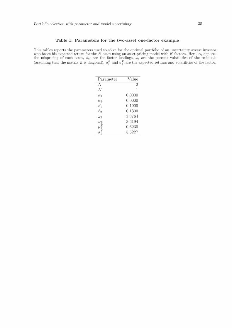
Portfolio selection with parameter and model uncertainty 35
Table 1: Parameters for the two-asset one-factor example
This tables reports the parameters used to solve for the optimal portfolio of an uncertainty averse investorwho bases his expected return for the N asset using an asset pricing model with K factors. Here, αi denotesthe mispricing of each asset, βij are the factor loadings, ωi are the percent volatilities of the residuals(assuming that the matrix Ω is diagonal), µF
j and σFj are the expected returns and volatilities of the factor.
Parameter ValueN 2K 1α1 0.0000α2 0.0000β1 0.1900β2 0.1300ω1 3.3764ω2 3.6194µF
1 0.6230σF
1 5.5227
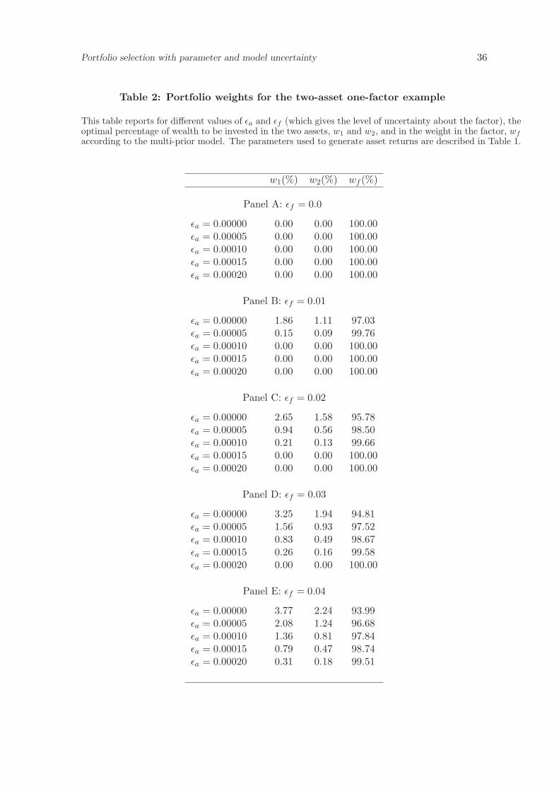
Portfolio selection with parameter and model uncertainty 36
Table 2: Portfolio weights for the two-asset one-factor example
This table reports for different values of εa and εf (which gives the level of uncertainty about the factor), theoptimal percentage of wealth to be invested in the two assets, w1 and w2, and in the weight in the factor, wf
according to the multi-prior model. The parameters used to generate asset returns are described in Table 1.
w1(%) w2(%) wf (%)
Panel A: εf = 0.0
εa = 0.00000 0.00 0.00 100.00εa = 0.00005 0.00 0.00 100.00εa = 0.00010 0.00 0.00 100.00εa = 0.00015 0.00 0.00 100.00εa = 0.00020 0.00 0.00 100.00
Panel B: εf = 0.01
εa = 0.00000 1.86 1.11 97.03εa = 0.00005 0.15 0.09 99.76εa = 0.00010 0.00 0.00 100.00εa = 0.00015 0.00 0.00 100.00εa = 0.00020 0.00 0.00 100.00
Panel C: εf = 0.02
εa = 0.00000 2.65 1.58 95.78εa = 0.00005 0.94 0.56 98.50εa = 0.00010 0.21 0.13 99.66εa = 0.00015 0.00 0.00 100.00εa = 0.00020 0.00 0.00 100.00
Panel D: εf = 0.03
εa = 0.00000 3.25 1.94 94.81εa = 0.00005 1.56 0.93 97.52εa = 0.00010 0.83 0.49 98.67εa = 0.00015 0.26 0.16 99.58εa = 0.00020 0.00 0.00 100.00
Panel E: εf = 0.04
εa = 0.00000 3.77 2.24 93.99εa = 0.00005 2.08 1.24 96.68εa = 0.00010 1.36 0.81 97.84εa = 0.00015 0.79 0.47 98.74εa = 0.00020 0.31 0.18 99.51
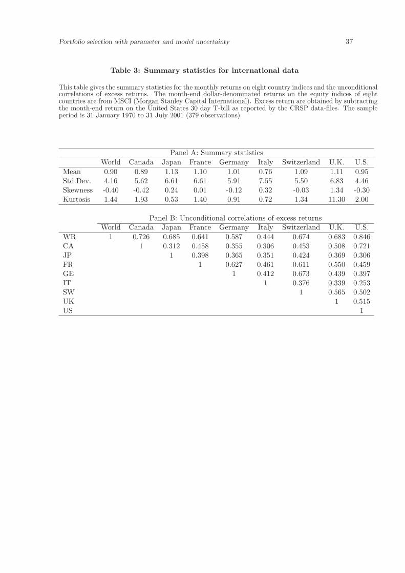
Portfolio selection with parameter and model uncertainty 37
Table 3: Summary statistics for international data
This table gives the summary statistics for the monthly returns on eight country indices and the unconditionalcorrelations of excess returns. The month-end dollar-denominated returns on the equity indices of eightcountries are from MSCI (Morgan Stanley Capital International). Excess return are obtained by subtractingthe month-end return on the United States 30 day T-bill as reported by the CRSP data-files. The sampleperiod is 31 January 1970 to 31 July 2001 (379 observations).
Panel A: Summary statisticsWorld Canada Japan France Germany Italy Switzerland U.K. U.S.
Mean 0.90 0.89 1.13 1.10 1.01 0.76 1.09 1.11 0.95Std.Dev. 4.16 5.62 6.61 6.61 5.91 7.55 5.50 6.83 4.46Skewness -0.40 -0.42 0.24 0.01 -0.12 0.32 -0.03 1.34 -0.30Kurtosis 1.44 1.93 0.53 1.40 0.91 0.72 1.34 11.30 2.00
Panel B: Unconditional correlations of excess returnsWorld Canada Japan France Germany Italy Switzerland U.K. U.S.
WR 1 0.726 0.685 0.641 0.587 0.444 0.674 0.683 0.846CA 1 0.312 0.458 0.355 0.306 0.453 0.508 0.721JP 1 0.398 0.365 0.351 0.424 0.369 0.306FR 1 0.627 0.461 0.611 0.550 0.459GE 1 0.412 0.673 0.439 0.397IT 1 0.376 0.339 0.253SW 1 0.565 0.502UK 1 0.515US 1

Portfolio selection with parameter and model uncertainty 38
Table 4: Out-of-sample performance of various portfolios using internationaldata
This table reports the out-of-sample Mean, Standard Deviation and Mean-to-Standard Deviation ratio forthe returns on different portfolio strategies. Means and Standard Deviations are expressed as percentageper month. The portfolio weights for each strategy are determined based using the international data basedon a data-window of 60 months and these portfolio weights are then used to calculate the returns in the61st month. The resulting out-of-sample period spans January 1975 to July 2001 (319 observations). Dataare described in Table 3. In parenthesis we report the percentage size of the confidence interval for a F8,52
implied by the values of ε.
Strategy Mean Std.Dev. MeanStd.Dev.
Panel A: Short sales allowedMean-Variance -0.517 42.085 -0.012
Minimum-Variance 1.090 4.116 0.265
Bayesian approachDiffuse Prior -0.491 41.394 -0.012Empirical Bayes-Stein -0.162 17.508 -0.009
Multi-prior approachε = 0 (0.00%) -0.517 42.085 -0.012ε = 1 (55.26%) 0.555 7.687 0.072ε = 3 (99.23%) 0.965 4.513 0.214ε = 5 (99.98%) 1.010 4.267 0.237ε = 10 (99.99%) 1.040 4.135 0.251ε →∞ (100%) 1.090 4.116 0.265
Panel B: Short sales not allowedMean-Variance 1.031 5.708 0.181
Minimum-Variance 1.100 4.007 0.274
Bayesian approach
Diffuse Prior 1.031 5.708 0.181Empirical Bayes-Stein 1.081 5.071 0.213
Multi-prior approachε = 0 (0.00%) 1.030 5.708 0.181ε = 1 (55.26%) 1.085 4.330 0.251ε = 3 (99.23%) 1.086 4.087 0.266ε = 5 (99.98%) 1.089 4.044 0.269ε = 10 (99.99%) 1.092 4.013 0.272ε →∞ (100%) 1.100 4.007 0.274
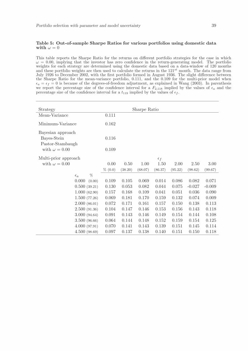
Portfolio selection with parameter and model uncertainty 39
Table 5: Out-of-sample Sharpe Ratios for various portfolios using domestic datawith ω = 0
This table reports the Sharpe Ratio for the returns on different portfolio strategies for the case in whichω = 0.00, implying that the investor has zero confidence in the return-generating model. The portfolioweights for each strategy are determined using the domestic data based on a data-window of 120 monthsand these portfolio weights are then used to calculate the returns in the 121st month. The data range fromJuly 1926 to December 2002, with the first portfolio formed in August 1936. The slight difference betweenthe Sharpe Ratio for the mean-variance portfolio, 0.111, and the 0.109 for the multi-prior model whenεa = εf = 0 is because of the degrees-of-freedom adjustment, as explained in Wang (2003). In parenthesiswe report the percentage size of the confidence interval for a F2,118 implied by the values of εa and thepercentage size of the confidence interval for a t119 implied by the values of εf .
Strategy Sharpe RatioMean-Variance 0.111
Minimum-Variance 0.162
Bayesian approachBayes-Stein 0.116Pastor-Stambaughwith ω = 0.00 0.109
Multi-prior approach εf
with ω = 0.00 0.00 0.50 1.00 1.50 2.00 2.50 3.00% (0.0) (38.20) (68.07) (86.37) (95.22) (98.62) (99.67)
εa %
0.000 (0.00) 0.109 0.105 0.069 0.014 0.086 0.082 0.0710.500 (39.21) 0.130 0.053 0.082 0.044 0.075 -0.027 -0.0091.000 (62.90) 0.157 0.168 0.109 0.041 0.051 0.036 0.0901.500 (77.26) 0.069 0.181 0.170 0.159 0.132 0.074 0.0092.000 (86.01) 0.072 0.171 0.161 0.157 0.150 0.138 0.1132.500 (91.36) 0.104 0.147 0.146 0.153 0.156 0.143 0.1183.000 (94.64) 0.091 0.143 0.146 0.149 0.154 0.144 0.1083.500 (96.66) 0.064 0.144 0.148 0.152 0.159 0.154 0.1254.000 (97.91) 0.070 0.141 0.143 0.139 0.151 0.145 0.1144.500 (98.69) 0.097 0.137 0.138 0.140 0.151 0.150 0.118
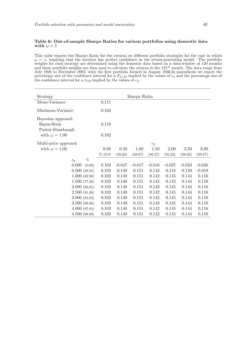
Portfolio selection with parameter and model uncertainty 40
Table 6: Out-of-sample Sharpe Ratios for various portfolios using domestic datawith ω = 1
This table reports the Sharpe Ratio for the returns on different portfolio strategies for the case in whichω = 1, implying that the investor has perfect confidence in the return-generating model. The portfolioweights for each strategy are determined using the domestic data based on a data-window of 120 monthsand these portfolio weights are then used to calculate the returns in the 121st month. The data range fromJuly 1926 to December 2002, with the first portfolio formed in August 1936.In parenthesis we report thepercentage size of the confidence interval for a F2,118 implied by the values of εa and the percentage size ofthe confidence interval for a t119 implied by the values of εf .
Strategy Sharpe RatioMean-Variance 0.111
Minimum-Variance 0.162
Bayesian approachBayes-Stein 0.116Pastor-Stambaughwith ω = 1.00 0.102
Multi-prior approach εf
with ω = 1.00 0.00 0.50 1.00 1.50 2.00 2.50 3.00% (0.0) (38.20) (68.07) (86.37) (95.22) (98.62) (99.67)
εa %
0.000 (0.00) 0.102 -0.047 -0.017 -0.016 -0.037 -0.023 -0.0260.500 (39.21) 0.102 0.140 0.151 0.142 0.144 0.139 -0.0181.000 (62.90) 0.102 0.140 0.151 0.142 0.145 0.144 0.1161.500 (77.26) 0.102 0.140 0.151 0.142 0.145 0.144 0.1162.000 (86.01) 0.102 0.140 0.151 0.142 0.145 0.144 0.1162.500 (91.36) 0.102 0.140 0.151 0.142 0.145 0.144 0.1163.000 (94.64) 0.102 0.140 0.151 0.142 0.145 0.144 0.1163.500 (96.66) 0.102 0.140 0.151 0.142 0.145 0.144 0.1164.000 (97.91) 0.102 0.140 0.151 0.142 0.145 0.144 0.1164.500 (98.69) 0.102 0.140 0.151 0.142 0.145 0.144 0.116
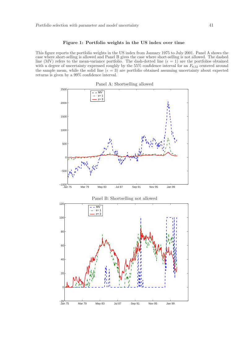
Portfolio selection with parameter and model uncertainty 41
Figure 1: Portfolio weights in the US index over time
This figure reports the portfolio weights in the US index from January 1975 to July 2001. Panel A shows thecase where short-selling is allowed and Panel B gives the case where short-selling is not allowed. The dashedline (MV) refers to the mean-variance portfolio. The dash-dotted line (ε = 1) are the portfolios obtainedwith a degree of uncertainty expressed roughly by the 55% confidence interval for an F8,52 centered aroundthe sample mean, while the solid line (ε = 3) are portfolio obtained assuming uncertainty about expectedreturns is given by a 99% confidence interval.
Panel A: Shortselling allowed
Jan 75 Mar 79 May 83 Jul 87 Sep 91 Nov 95 Jan 99 −1000
−500
0
500
1000
1500
2000
2500MV ε= 1ε= 3
Panel B: Shortselling not allowed
Jan 75 Mar 79 May 83 Jul 87 Sep 91 Nov 95 Jan 99 −20
0
20
40
60
80
100
120MV ε= 1ε= 3
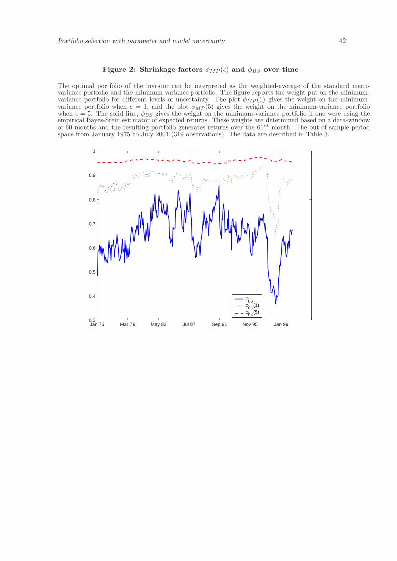
Portfolio selection with parameter and model uncertainty 42
Figure 2: Shrinkage factors φMP (ε) and φBS over time
The optimal portfolio of the investor can be interpreted as the weighted-average of the standard mean-variance portfolio and the minimum-variance portfolio. The figure reports the weight put on the minimum-variance portfolio for different levels of uncertainty. The plot φMP (1) gives the weight on the minimum-variance portfolio when ε = 1, and the plot φMP (5) gives the weight on the minimum-variance portfoliowhen ε = 5. The solid line, φBS gives the weight on the minimum-variance portfolio if one were using theempirical Bayes-Stein estimator of expected returns. These weights are determined based on a data-windowof 60 months and the resulting portfolio generates returns over the 61st month. The out-of sample periodspans from January 1975 to July 2001 (319 observations). The data are described in Table 3.
Jan 75 Mar 79 May 83 Jul 87 Sep 91 Nov 95 Jan 99 0.3
0.4
0.5
0.6
0.7
0.8
0.9
1
φBS
φ
PU(1)
φPU
(5)

Portfolio selection with parameter and model uncertainty 43
Figure 3: Portfolio weights assuming expected returns estimated using MLE
The figure has four panels (two on this page and two on the next) which report the weight over time in SMB,HML, MKT and the riskfree asset. Expected returns are estimated using the maximum-likelihood estimatorusing a rolling window estimation period of 120 months. The data range from July 1926 to December 2002.The first portfolio is formed in August 1936. The plots on the left hand side refer to the case of no uncertaintyin the market (εf = 0), while the plots on the right hand side assume a level of uncertainty in the marketequal to εf = 2. In each figure we consider three different level of uncertainty about the asset estimate:εa = 0 (dash-dotted), εa = 0.5 (dotted), εa = 4.5 (dashed). The solid black line represents the portfoliochosen by a single-prior Bayesian who places infinite confidence in the data (ω = 0).
Panel A: Portfolio weights in SMBεf = 0.00 εf = 2.00
Jul36 Nov44 Mar53 Jun61 Oct69 Feb78 May86 Sep94 Dec02−0.2
−0.15
−0.1
−0.05
0
0.05
0.1
0.15
εa=0
εa=0.5
εa=4.5
Bayes, ω=0
Jul36 Nov44 Mar53 Jun61 Oct69 Feb78 May86 Sep94 Dec02−0.2
−0.15
−0.1
−0.05
0
0.05
0.1
0.15
εa=0
εa=0.5
εa=4.5
Bayes, ω=0
Panel B: Portfolio weights in HMLεf = 0.00 εf = 2.00
Jul36 Nov44 Mar53 Jun61 Oct69 Feb78 May86 Sep94 Dec02−0.04
−0.02
0
0.02
0.04
0.06
0.08
0.1
0.12
0.14
0.16
εa=0
εa=0.5
εa=4.5
Bayes, ω=0
Jul36 Nov44 Mar53 Jun61 Oct69 Feb78 May86 Sep94 Dec02−0.04
−0.02
0
0.02
0.04
0.06
0.08
0.1
0.12
0.14
0.16
εa=0
εa=0.5
εa=4.5
Bayes, ω=0

Portfolio selection with parameter and model uncertainty 44
Panel C: Portfolio weights in MKTεf = 0.00 εf = 2.00
Jul36 Nov44 Mar53 Jun61 Oct69 Feb78 May86 Sep94 Dec02−0.04
−0.02
0
0.02
0.04
0.06
0.08
0.1
0.12
0.14
0.16
εa=0
εa=0.5
εa=4.5
Bayes, ω=0
Jul36 Nov44 Mar53 Jun61 Oct69 Feb78 May86 Sep94 Dec02−0.04
−0.02
0
0.02
0.04
0.06
0.08
0.1
0.12
0.14
0.16
εa=0
εa=0.5
εa=4.5
Bayes, ω=0
Panel D: Portfolio weights in the riskfree assetεf = 0.00 εf = 2.00
Jul36 Nov44 Mar53 Jun61 Oct69 Feb78 May86 Sep94 Dec020.7
0.75
0.8
0.85
0.9
0.95
1
1.05
εa=0
εa=0.5
εa=4.5
Bayes, ω=0
Jul36 Nov44 Mar53 Jun61 Oct69 Feb78 May86 Sep94 Dec020.7
0.75
0.8
0.85
0.9
0.95
1
1.05
1.1
εa=0
εa=0.5
εa=4.5
Bayes, ω=0
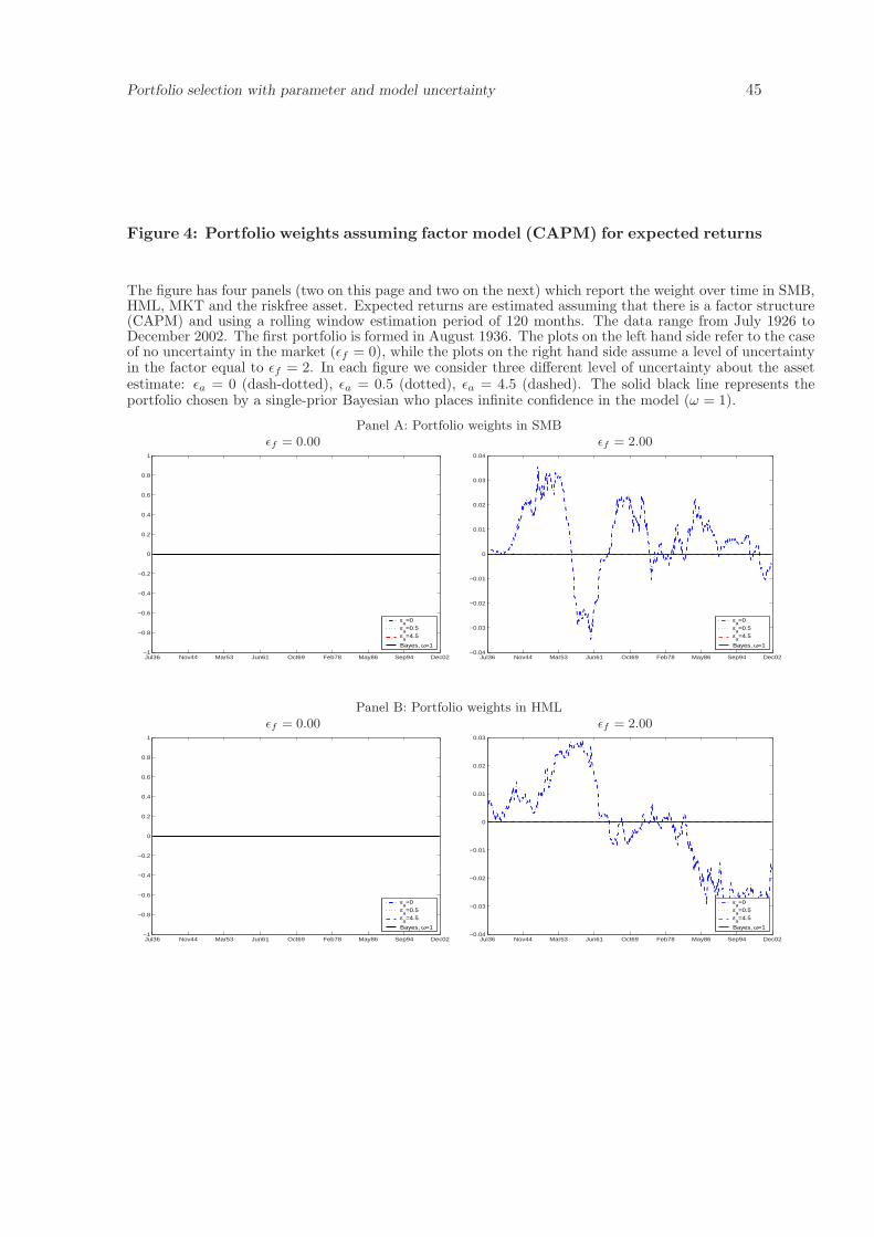
Portfolio selection with parameter and model uncertainty 45
Figure 4: Portfolio weights assuming factor model (CAPM) for expected returns
The figure has four panels (two on this page and two on the next) which report the weight over time in SMB,HML, MKT and the riskfree asset. Expected returns are estimated assuming that there is a factor structure(CAPM) and using a rolling window estimation period of 120 months. The data range from July 1926 toDecember 2002. The first portfolio is formed in August 1936. The plots on the left hand side refer to the caseof no uncertainty in the market (εf = 0), while the plots on the right hand side assume a level of uncertaintyin the factor equal to εf = 2. In each figure we consider three different level of uncertainty about the assetestimate: εa = 0 (dash-dotted), εa = 0.5 (dotted), εa = 4.5 (dashed). The solid black line represents theportfolio chosen by a single-prior Bayesian who places infinite confidence in the model (ω = 1).
Panel A: Portfolio weights in SMBεf = 0.00 εf = 2.00
Jul36 Nov44 Mar53 Jun61 Oct69 Feb78 May86 Sep94 Dec02−1
−0.8
−0.6
−0.4
−0.2
0
0.2
0.4
0.6
0.8
1
εa=0
εa=0.5
εa=4.5
Bayes, ω=1
Jul36 Nov44 Mar53 Jun61 Oct69 Feb78 May86 Sep94 Dec02−0.04
−0.03
−0.02
−0.01
0
0.01
0.02
0.03
0.04
εa=0
εa=0.5
εa=4.5
Bayes, ω=1
Panel B: Portfolio weights in HMLεf = 0.00 εf = 2.00
Jul36 Nov44 Mar53 Jun61 Oct69 Feb78 May86 Sep94 Dec02−1
−0.8
−0.6
−0.4
−0.2
0
0.2
0.4
0.6
0.8
1
εa=0
εa=0.5
εa=4.5
Bayes, ω=1
Jul36 Nov44 Mar53 Jun61 Oct69 Feb78 May86 Sep94 Dec02−0.04
−0.03
−0.02
−0.01
0
0.01
0.02
0.03
εa=0
εa=0.5
εa=4.5
Bayes, ω=1
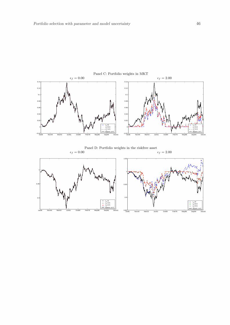
Portfolio selection with parameter and model uncertainty 46
Panel C: Portfolio weights in MKTεf = 0.00 εf = 2.00
Jul36 Nov44 Mar53 Jun61 Oct69 Feb78 May86 Sep94 Dec02−0.02
0
0.02
0.04
0.06
0.08
0.1
0.12
0.14
εa=0
εa=0.5
εa=4.5
Bayes, ω=1
Jul36 Nov44 Mar53 Jun61 Oct69 Feb78 May86 Sep94 Dec02−0.02
0
0.02
0.04
0.06
0.08
0.1
0.12
0.14
εa=0
εa=0.5
εa=4.5
Bayes, ω=1
Panel D: Portfolio weights in the riskfree assetεf = 0.00 εf = 2.00
Jul36 Nov44 Mar53 Jun61 Oct69 Feb78 May86 Sep94 Dec02
0.9
0.95
1
εa=0
εa=0.5
εa=4.5
Bayes, ω=1
Jul36 Nov44 Mar53 Jun61 Oct69 Feb78 May86 Sep94 Dec020.85
0.9
0.95
1
1.05
εa=0
εa=0.5
εa=4.5
Bayes, ω=1

Portfolio selection with parameter and model uncertainty 47
References
Anderson, E., L. Hansen, and T. Sargent, 1999, “Robustness detection and the price ofrisk,” Working paper, University of Chicago.
Barry, C. B., 1974, “Portfolio Analysis under Uncertain Means, Variances, and Covari-ances,” Journal of Finance, 29, 515–22.
Bawa, V. S., S. Brown, and R. Klein, 1979, Estimation Risk and Optimal Portfolio Choice,North Holland, Amsterdam.
Berger, J., 1974, “Minimax Estimator of a Multivariate Normal Mean Under PolynomialLoss,” Journal of Multivariate Analysis, 8, 173–180.
Best, M. J., and R. R. Grauer, 1991, “On the Sensitivity of Mean-Variance-Efficient Portfo-lios to Changes in Asset Means: Some Analytical and Computational Results,” Reviewof Financial Studies, 4, 315–42.
Best, M. J., and R. R. Grauer, 1992, “Positively Weighted Minimum-Variance Portfoliosand the Structure of Asset Expected Returns,” Journal of Financial and QuantitativeAnalysis, 27, 513–37.
Bewley, T., 1988, “Knightian Decision Theory and Econometric Inference,” Working Paper,Yale University.
Black, F., and R. Litterman, 1990, “Asset Allocation: Combining Investor Views withMarket Equilibrium,” Discussion paper, Goldman, Sachs & Co.
Black, F., and R. Litterman, 1992, “Global Portfolio Optimization,” Financial AnalystsJournal, 48, 28–43.
Chan, L. K. C., J. Karceski, and J. Lakonishok, 1999, “On Portfolio Optimization: Fore-casting Covariances and Choosing the Risk Model,” Review of Financial Studies, 12,937–74.
Chen, Z., and L. Epstein, 2002, “Ambiguity, Risk, and Asset Returns in Continuous Time,”Econometrica, 70, 1403–43.
Chopra, V. K., 1993, “Improving Optimization,” Journal of Investing, 8, 51–59.
Chopra, V. K., and W. T. Ziemba, 1993, “The Effect of Errors in Means, Variances, andCovariances on Optimal Portfolio Choice,” Journal of Portfolio Management, 19, 6–11.
De Santis, G., and B. Gerard, 1997, “International Asset Pricing and Portfolio Diversifica-tion with Time-Varying Risk,” Journal of Finance, 52, 1881–1912.
Dow, J., and S. R. d. C. Werlang, 1992, “Uncertainty Aversion, Risk Aversion, and theOptimal Choice of Portfolio,” Econometrica, 60, 197–204.
Dumas, B., and B. Jacquillat, 1990, “Performance of Currency Portfolios Chosen by aBayesian Technique: 1967-1985,” Journal of Banking and Finance, 14, 539–58.
Ellsberg, D., 1961, “Risk, Ambiguity and the Savage Axioms,” Quarterly Journal of Eco-nomics, 75, 643–669.

Portfolio selection with parameter and model uncertainty 48
Epstein, L. G., and T. Wang, 1994, “Intertemporal Asset Pricing Under Knightian Uncer-tainty,” Econometrica, 62, 283–322.
Fox, C., and A. Tversky, 1995, “Ambiguity Aversion and Comparative Ignorance,” Quar-terly Journal of Economics, 110, 585–603.
Frost, P., and J. Savarino, 1988, “For Better Performance Constrain Portfolio Weights,”Journal of Portfolio Management, 15, 29–34.
Frost, P. A., and J. E. Savarino, 1986, “An Empirical Bayes Approach to Efficient PortfolioSelection,” Journal of Financial and Quantitative Analysis, 21, 293–305.
Gilboa, I., and D. Schmeidler, 1989, “Maxmin Expected Utility Theory with Non-UniquePrior,” Journal of Mathematical Economics, 18, 141–153.
Goldfarb, D., and G. Iyengar, 2003, “Robust Portfolio Selection Problems,” Mathematicaof Operations Research, 28, 1–38.
Halldorsson, B., and R. Tutuncu, 2000, “An Interior-Point Method for a Class of SaddlePoint Problems,” Working Paper, Carnegie Mellon University.
Harvey, C. R., J. Liechty, M. Liechty, and P. Muller, 2003, “Portfolio Selection with HigherMoments,” Working Paper, Duke University.
Heath, C., and A. Tversky, 1991, “Preferences and Beliefs: Ambiguity and Competence inChoice under Uncertainty,” Journal of Risk and Uncertainty, 4, 5–28.
Hodges, S. D., and R. A. Brealey, 1978, “Portfolio Selection in a Dynamic and UncertinWorld,” in James H. Lorie, and R. A. Brealey (ed.), Modern Developments in Invest-ment Management, Dryden Press, Hinsdale, Illionois, 2nd edn.
Jagannathan, R., and T. Ma, 2003, “Risk Reduction in Large Portfolios: Why Imposingthe Wrong Constraints Helps,” Journal of Finance, 58, 1651–1684.
Jobson, J. D., and R. Korkie, 1980, “Estimation for Markowitz Efficient Portfolios,” Journalof the American Statistical Association, 75, 544–554.
Johnson, R., and D. W. Wichern, 1992, Applied Multivariate Statistical Analysis, PrenticeHall.
Jorion, P., 1985, “International Portfolio Diversification with Estimation Risk,” Journal ofBusiness, 58, 259–278.
Jorion, P., 1986, “Bayes-Stein Estimation for Portfolio Analysis,” Journal of Financial andQuantitative Analysis, 21, 279–92.
Klein, R. W., and V. S. Bawa, 1976, “The Effect of Estimation Risk on Optimal PortfolioChoice,” Journal of Financial Economics, 3, 215–31.
Knight, F., 1921, Risk, Uncertainty and Profit, Houghton Mifflin, Boston.
Kogan, L., and T. Wang, 2002, “A Simple Theory of Asset Pricing under Model Uncer-tainty,” Working Paper, University of British Columbia.
Ledoit, O., 1996, “A Well-Conditioned Estimator for Large-Dimensional Covariance Matri-ces,” Working Paper, Anderson School, UCLA.
Portfolio selection with parameter and model uncertainty 49
Ledoit, O., and M. Wolf, 2003, “Honey, I Shrunk the Sample Covariance Matrix,” WorkingPaper, Department of Economics and Business, Universitat Pompeu Fabra.
Litterman, R., 2003, Modern Investment Management: An Equilibrium Approach, Wiley.
Markowitz, H. M., 1952, “Mean-Variance Analysis in Portfolio Choice and Capital Mar-kets,” Journal of Finance, 7, 77–91.
Markowitz, H. M., 1959, Portfolio Selection, Wiley, New York.
Merton, R., 1980, “On estimating the expected return on the market: An exploratoryinvestigation,” Journal of Financial Economics, 8, 323–361.
Michaud, R. O., 1989, “The Markowitz Optimization Enigma: Is Optimized Optimal,”Financial Analysts Journal, 45, 31–42.
Michaud, R. O., 1998, Efficient Asset Management, Harvard Business School Press, Boston.
Pastor, L., 2000, “Portfolio Selection and Asset Pricing Models,” Journal of Finance, 55,179–223.
Pastor, L., and R. F. Stambaugh, 2000, “Comparing Asset Pricing Models: An InvestmentPerspective,” Journal of Financial Economics, 56, 335–81.
Scherer, B., 2002, “Portfolio Resampling: Review and Critique,” Financial Analysts Jour-nal, 58, 98–109.
Sharpe, W. F., 1970, Portfolio Theory and Capital Markets, McGraw-Hill, New York.
Stambaugh, R. F., 1997, “Analyzing Investments whose Histories Differ in Length,” Journalof Financial Economics, 45, 285–331.
Stein, C., 1955, “Inadmissibility of the Usual Estimator for the Mean of a MultivariateNormal Distribution,” in 3rd Berkely Symposium on Probability and Statistics, , vol. 1,pp. 197–206, Berkeley. University of California Press.
Tutuncu, R., and M. Koenig, 2003, “Robust Asset Allocation,” Working Paper, CarnegieMellon University.
Uppal, R., and T. Wang, 2003, “Model Misspecification and Underdiversification,” Journalof Finance, 58, 2465–2486.
Wang, Z., 2003, “A Shrinkage Approach to Model Uncertainty and Asset Allocation,”Working Paper, Columbia University.