portfolio optimization: analytical … course iii/6 portfolio... · 3. solving the portfolio...
TRANSCRIPT

Keith Brown, Ph.D., CFA
November 22nd, 2007
PORTFOLIO OPTIMIZATION: PORTFOLIO OPTIMIZATION: ANALYTICAL TECHNIQUESANALYTICAL TECHNIQUES
1
• The preceding analysis demonstrates that it is possible for investors to reduce their risk exposure simply by holding in their portfolios a sufficiently large number of assets (or asset classes). This is the notion of naïve diversification, but as we have seen there is a limit to how much risk this process can remove.
• Efficient diversification is the process of selecting portfolio holdings so as to: (i) minimize portfolio risk while (ii) achieving expected return objectives and, possibly, satisfying other constraints (e.g., no short sales allowed). Thus, efficient diversification is ultimately a constrained optimization problem. We will return to this topic in the next session.
• Notice that simply minimizing portfolio risk without a specific return objective in mind (i.e., an unconstrained optimization problem) is seldom interesting to an investor. After all, in an efficient market, any riskless portfolio should just earn the risk-free rate, which the investor could obtain more cost-effectively with a T-bill purchase.
Overview of the Portfolio Optimization Process
2
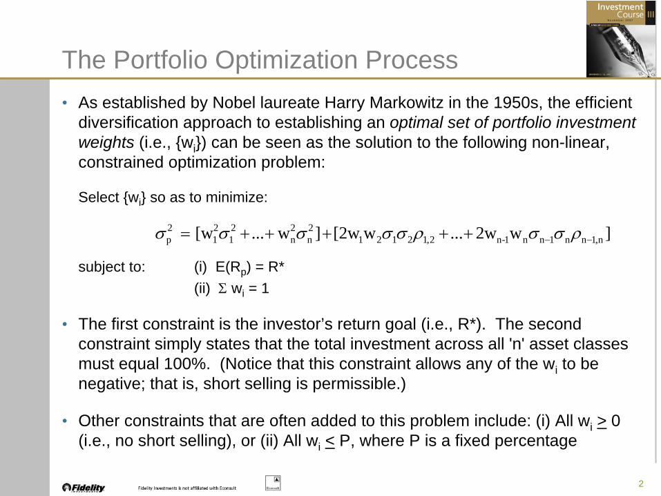
The Portfolio Optimization Process• As established by Nobel laureate Harry Markowitz in the 1950s, the efficient
diversification approach to establishing an optimal set of portfolio investment weights (i.e., {wi }) can be seen as the solution to the following non-linear, constrained optimization problem:
Select {wi } so as to minimize:
subject to: (i) E(Rp ) = R*(ii) Σ
wi = 1
• The first constraint is the investor’s return goal (i.e., R*). The second constraint simply states that the total investment across all 'n' asset classes must equal 100%. (Notice that this constraint allows any of the wi to be negative; that is, short selling is permissible.)
• Other constraints that are often added to this problem include: (i) All wi > 0 (i.e., no short selling), or (ii) All wi < P, where P is a fixed percentage
]w2w ... w[2w ] w ... [w n,1nn1nn1-n2,121212n
2n
21
21
2p −−+++++= ρσσρσσσσσ
3
Solving the Portfolio Optimization Problem
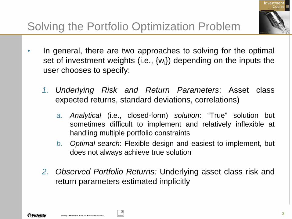
• In general, there are two approaches to solving for the optimal set of investment weights (i.e., {wi }) depending on the inputs the user chooses to specify:
1. Underlying Risk and Return Parameters: Asset class expected returns, standard deviations, correlations)
a. Analytical (i.e., closed-form) solution: “True” solution but sometimes difficult to implement and relatively inflexible at handling multiple portfolio constraints
b. Optimal search: Flexible design and easiest to implement, but does not always achieve true solution
2. Observed Portfolio Returns: Underlying asset class risk and return parameters estimated implicitly
4
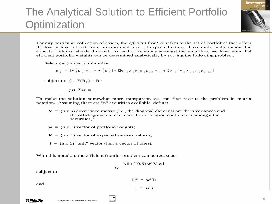
For any particular collection of assets, the efficient frontier refers to the set of portfolios that offers the lowest level of risk for a pre-specified level of expected return. Given information about theexpected returns, standard deviations, and correlations amongst the securities, we have seen thatefficient portfolio weights can be determined analytically by solving the following problem: Select {wi} so as to minimize:
subject to: (i) E(Rp) = R* (ii) Σwi = 1. To make the solution somewhat more transparent, we can first rewrite the problem in matrixnotation. Assuming there are "n" securities available, define: V = (n x n) covariance matrix (i.e., the diagonal elements are the n variances and the off-diagonal elements are the correlation coefficients amongst the securities); w = (n x 1) vector of portfolio weights; R = (n x 1) vector of expected security returns; i = (n x 1) "unit" vector (i.e., a vector of ones). With this notation, the efficient frontier problem can be recast as:
Min [(0.5) w' V w] w subject to
R* = w' R and
1 = w' i
]w2w ... w[2w ] w ... [w n,1nn1nn1-n2,121212n
2n
21
21
2p −−+++++= ρσσρσσσσσ
The Analytical Solution to Efficient Portfolio Optimization
5
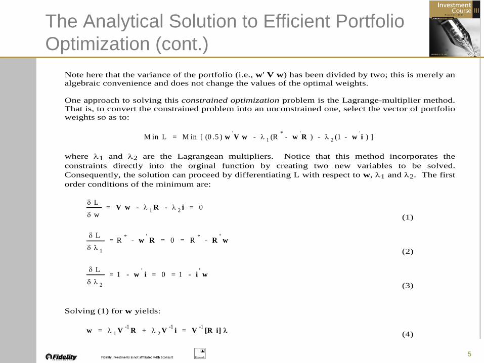
Note here that the variance of the portfolio (i.e., w' V w) has been divided by two; this is merely an algebraic convenience and does not change the values of the optimal weights. One approach to solving this constrained optimization problem is the Lagrange-multiplier method. That is, to convert the constrained problem into an unconstrained one, select the vector of portfolio weights so as to:
M in L = M in [ (0 .5 ) w 'V w - λ 1 (R * - w 'R ) - λ 2 (1 - w 'i ) ] where λ1 and λ2 are the Lagrangean multipliers. Notice that this method incorporates the constraints directly into the orginal function by creating two new variables to be solved.Consequently, the solution can proceed by differentiating L with respect to w, λ1 and λ2. The first order conditions of the minimum are:
δ L
δ w= V w - λ 1 R - λ 2 i = 0
(1)
δ L
δ λ 1
= R * - w ' R = 0 = R * - R ' w (2)
δ L
δ λ 2
= 1 - w ' i = 0 = 1 - i ' w (3)
Solving (1) for w yields:
w = λ 1 V -1 R + λ 2 V -1 i = V -1 [R i] λ (4)
The Analytical Solution to Efficient Portfolio Optimization (cont.)
6
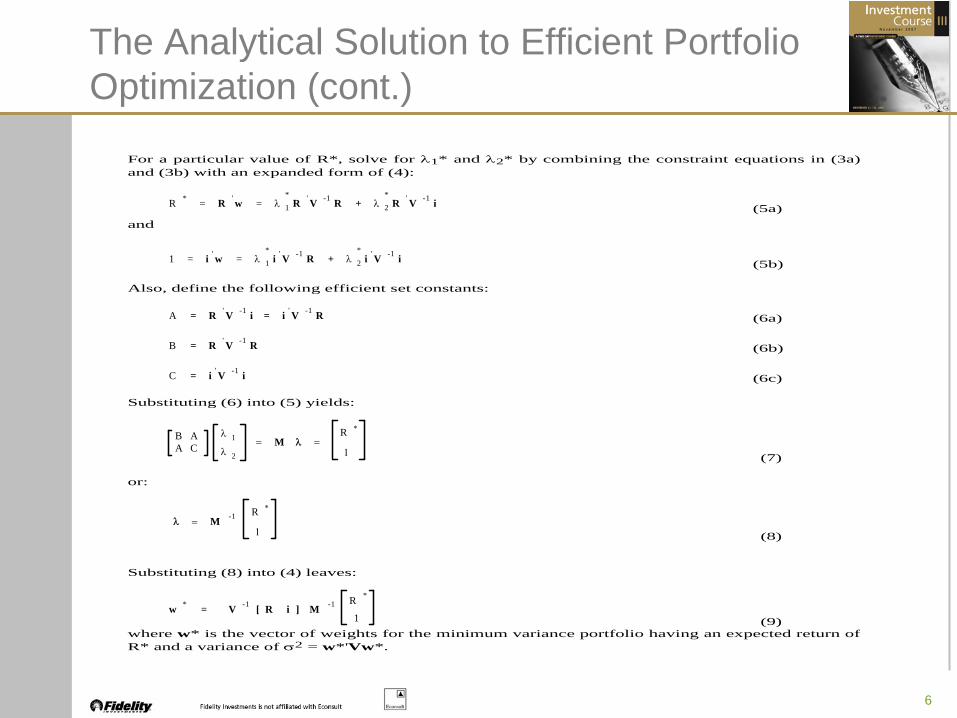
For a particular value of R*, solve for λ1* and λ2* by combining the constraint equations in (3a)and (3b) with an expanded form of (4):
R * = R ' w = λ 1
*R ' V -1 R + λ 2
*R ' V -1 i (5a)
and
1 = i ' w = λ 1
*i ' V -1 R + λ 2
*i ' V -1 i (5b)
Also, define the following efficient set constants:
A = R ' V -1 i = i ' V -1 R (6a)
B = R ' V -1 R (6b)
C = i ' V -1 i (6c) Substituting (6) into (5) yields:
B AA C
λ 1
λ 2
= M λ =R ∗
1 (7) or:
λ = M -1 R ∗
1 (8) Substituting (8) into (4) leaves:
w * = V -1 [ R i ] M -1 R *
1 (9) where w* is the vector of weights for the minimum variance portfolio having an expected return ofR* and a variance of σ2 = w*'Vw*.
The Analytical Solution to Efficient Portfolio Optimization (cont.)
7
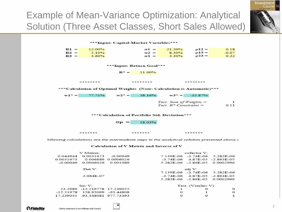
Example of Mean-Variance Optimization: Analytical Solution (Three Asset Classes, Short Sales Allowed)
8
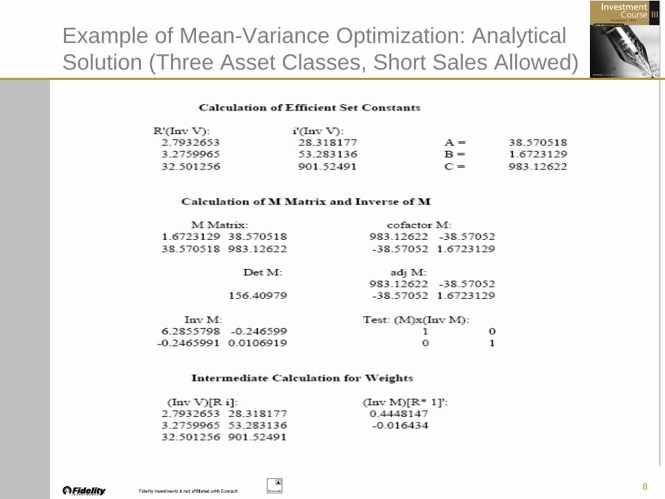
Example of Mean-Variance Optimization: Analytical Solution (Three Asset Classes, Short Sales Allowed)
9
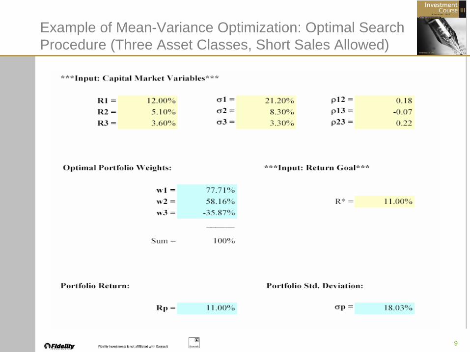
Example of Mean-Variance Optimization: Optimal Search Procedure (Three Asset Classes, Short Sales Allowed)
10
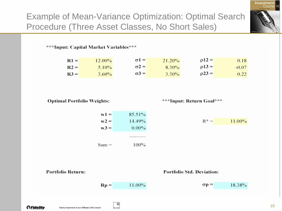
Example of Mean-Variance Optimization: Optimal Search Procedure (Three Asset Classes, No Short Sales)

11
• Main Idea: Any constraint on the optimization process imposes a cost to the investor in terms of incremental portfolio volatility, but only if that constraint is binding (i.e., keeps you from investing in an otherwise optimal manner).
Measuring the Cost of Constraint: Incremental Portfolio Risk

12
Mean-Variance Efficient Frontier With and Without Short-Selling

13
Optimal Search Efficient Frontier Example: Five Asset Classes
14
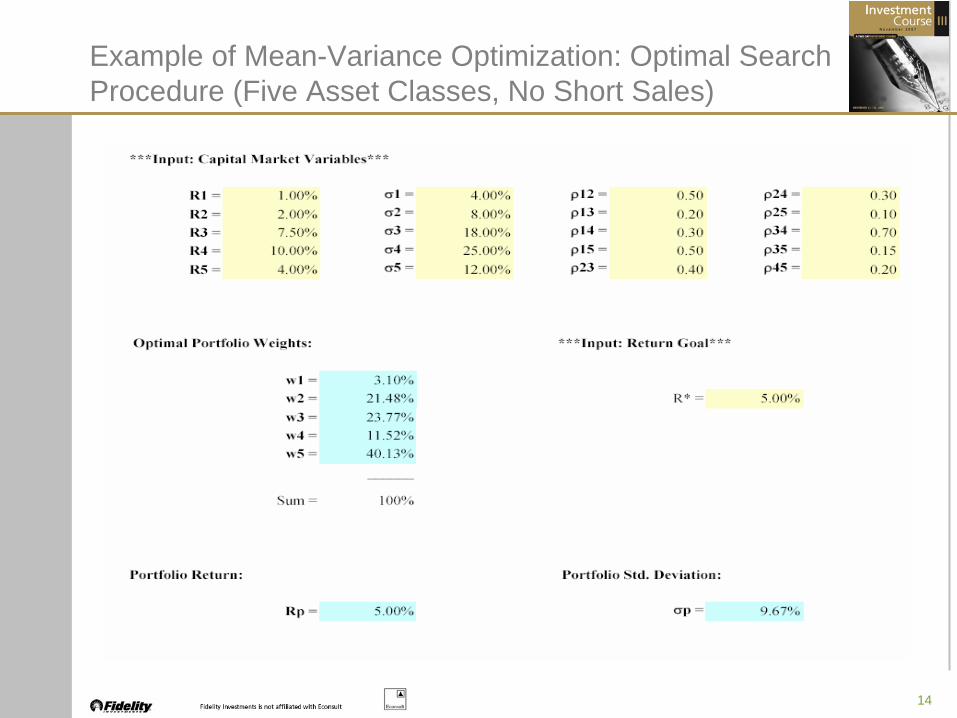
Example of Mean-Variance Optimization: Optimal Search Procedure (Five Asset Classes, No Short Sales)
15
Mean-Variance Optimization with Black-Litterman Inputs
• One of the criticisms that is sometimes made about the mean- variance optimization process that we have just seen is that the inputs (e.g., asset class expected returns, standard deviations, and correlations) must be estimated, which can effect the quality of the resulting strategic allocations.
• Typically, these inputs are estimated from historical return data. However, it has been observed that inputs estimated with historical data—the expected returns, in particular—lead to “extreme” portfolio allocations that do not appear to be realistic.
• Black-Litterman expected returns are often preferred in practice for the use in mean-variance optimizations because the equilibrium- consistent forecasts lead to “smoother”, more realistic allocations.
16
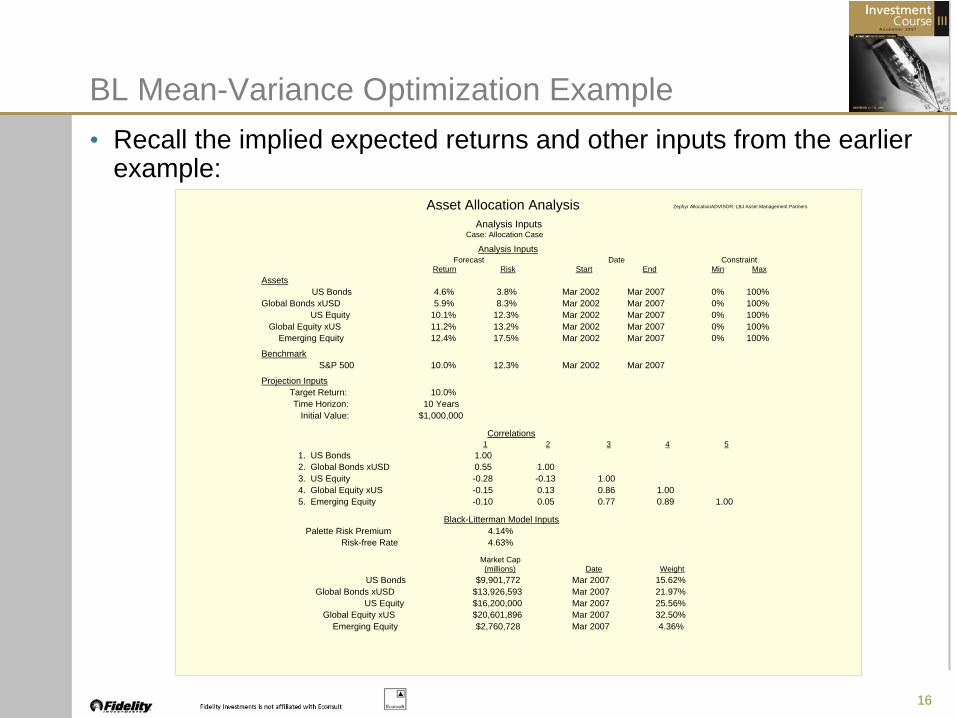
BL Mean-Variance Optimization Example• Recall the implied expected returns and other inputs from the earlier
example:Asset Allocation Analysis Zephyr AllocationADVISOR: LBJ Asset Management Partners
Analysis InputsCase: Allocation Case
Analysis InputsForecast Date Constraint
Return Risk Start End Min MaxAssets
US Bonds 4.6% 3.8% Mar 2002 Mar 2007 0% 100%Global Bonds xUSD 5.9% 8.3% Mar 2002 Mar 2007 0% 100%
US Equity 10.1% 12.3% Mar 2002 Mar 2007 0% 100%Global Equity xUS 11.2% 13.2% Mar 2002 Mar 2007 0% 100%
Emerging Equity 12.4% 17.5% Mar 2002 Mar 2007 0% 100%
BenchmarkS&P 500 10.0% 12.3% Mar 2002 Mar 2007
Projection InputsTarget Return: 10.0%Time Horizon: 10 Years
Initial Value: $1,000,000
Correlations1 2 3 4 5
1. US Bonds 1.002. Global Bonds xUSD 0.55 1.003. US Equity -0.28 -0.13 1.004. Global Equity xUS -0.15 0.13 0.86 1.005. Emerging Equity -0.10 0.05 0.77 0.89 1.00
Black-Litterman Model InputsPalette Risk Premium 4.14%
Risk-free Rate 4.63%
Market Cap(millions) Date Weight
US Bonds $9,901,772 Mar 2007 15.62%Global Bonds xUSD $13,926,593 Mar 2007 21.97%
US Equity $16,200,000 Mar 2007 25.56%Global Equity xUS $20,601,896 Mar 2007 32.50%
Emerging Equity $2,760,728 Mar 2007 4.36%
17
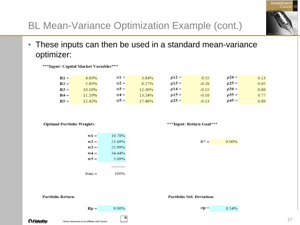
BL Mean-Variance Optimization Example (cont.)
• These inputs can then be used in a standard mean-variance optimizer:
18
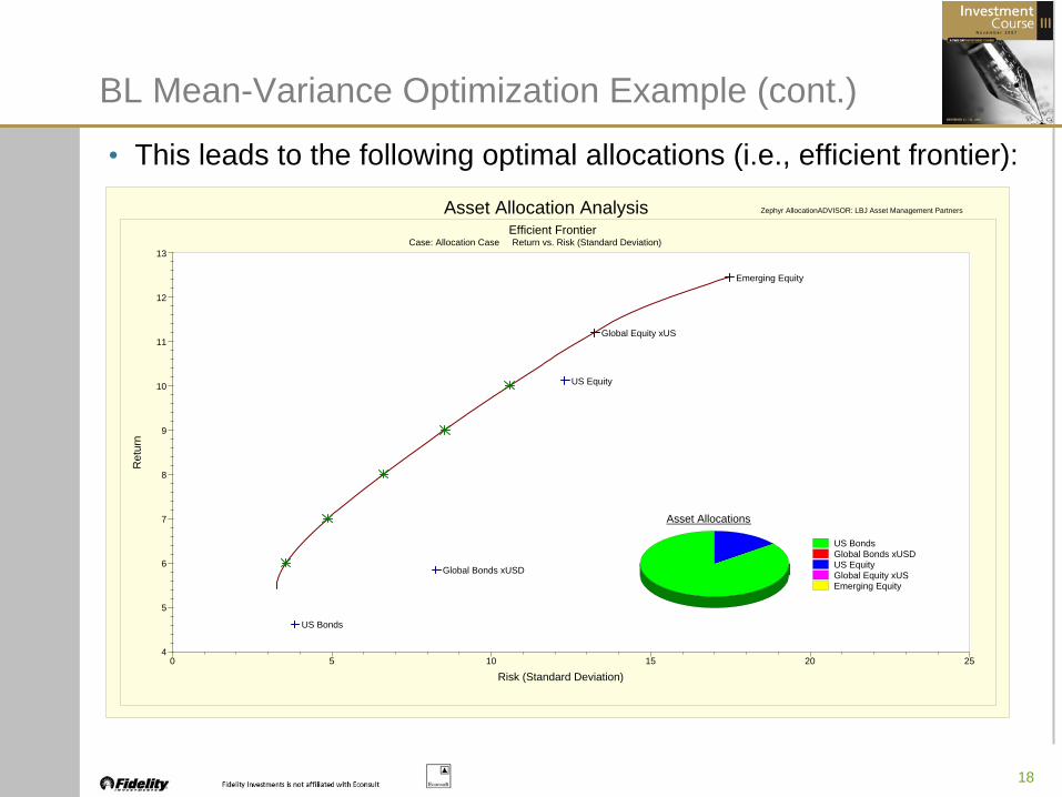
• This leads to the following optimal allocations (i.e., efficient frontier):Asset Allocation Analysis Zephyr AllocationADVISOR: LBJ Asset Management Partners
Efficient FrontierCase: Allocation Case Return vs. Risk (Standard Deviation)
0 5 10 15 20 254
5
6
7
8
9
10
11
12
13
Risk (Standard Deviation)
Ret
urn
US BondsGlobal Bonds xUSDUS EquityGlobal Equity xUSEmerging Equity
Asset Allocations
US Bonds
Global Bonds xUSD
US Equity
Global Equity xUS
Emerging Equity
BL Mean-Variance Optimization Example (cont.)
19
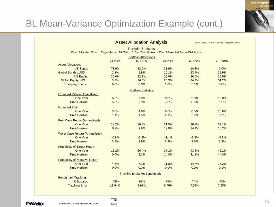
Asset Allocation Analysis Zephyr AllocationADVISOR: LBJ Asset Management Partners
Portfolio StatisticsCase: Allocation Case Target Return: 10.00% - 10 Year Time Horizon - 95% of Projected Return Distribution
Portfolio AllocationsE(R)=6% E(R)=7% E(R)=8% E(R)=9% E(R)=10%
Asset AllocationsUS Bonds 73.9% 52.9% 31.9% 10.8% 0.0%
Global Bonds xUSD 2.2% 8.9% 16.1% 23.7% 19.9%US Equity 20.6% 22.1% 23.9% 26.0% 20.8%
Global Equity xUS 3.3% 16.0% 26.3% 34.4% 51.2%Emerging Equity 0.0% 0.0% 1.8% 5.1% 8.0%
Portfolio StatisticsExpected Return (Annualized)
One Year 6.0% 7.0% 8.0% 9.0% 10.0%Time Horizon 5.9% 6.9% 7.8% 8.7% 9.5%
Expected RiskOne Year 3.6% 4.9% 6.6% 8.5% 10.6%
Time Horizon 1.1% 1.5% 2.1% 2.7% 3.3%
Best Case Return (Annualized)One Year 13.2% 16.8% 21.5% 26.7% 32.1%
Time Horizon 8.2% 9.9% 12.0% 14.1% 16.2%
Worst Case Return (Annualized)One Year -0.8% -2.2% -4.4% -6.8% -9.3%
Time Horizon 3.8% 3.9% 3.8% 3.5% 3.2%
Probability of Target ReturnOne Year 13.2% 26.4% 37.1% 43.8% 48.1%
Time Horizon 0.0% 2.3% 14.8% 31.1% 44.0%
Probability of Negative ReturnOne Year 4.3% 7.1% 11.0% 14.4% 17.2%
Time Horizon 0.0% 0.0% 0.0% 0.0% 0.1%
Tracking to Market BenchmarkBenchmark Tracking
R-Squared 48% 69% 74% 74% 73%Tracking Error 11.64% 9.92% 8.48% 7.51% 7.25%
BL Mean-Variance Optimization Example (cont.)

20
• Another advantage of the BL Optimization model is that it provides a way for the user to incorporate his own views about asset class expected returns into the estimation of the efficient frontier.
• Said differently, if you do not agree with the implied returns, the BL model allows you to make tactical adjustments to the inputs and still achieve well-diversified portfolios that reflect your view.
• Two components of a tactical view:
Asset Class Performance- Absolute (e.g., Asset Class #1 will have a return of X%)- Relative (e.g., Asset Class #1 will outperform Asset Class #2 by Y%)
User Confidence Level- 0% to 100%, indicating certainty of return view
(See the article “A Step-by-Step Guide to the Black-Litterman Model” by T. Idzorek of Zephyr Associates for more details on the computational process involved with incorporating user- specified tactical views)
BL Mean-Variance Optimization Example (cont.)
21
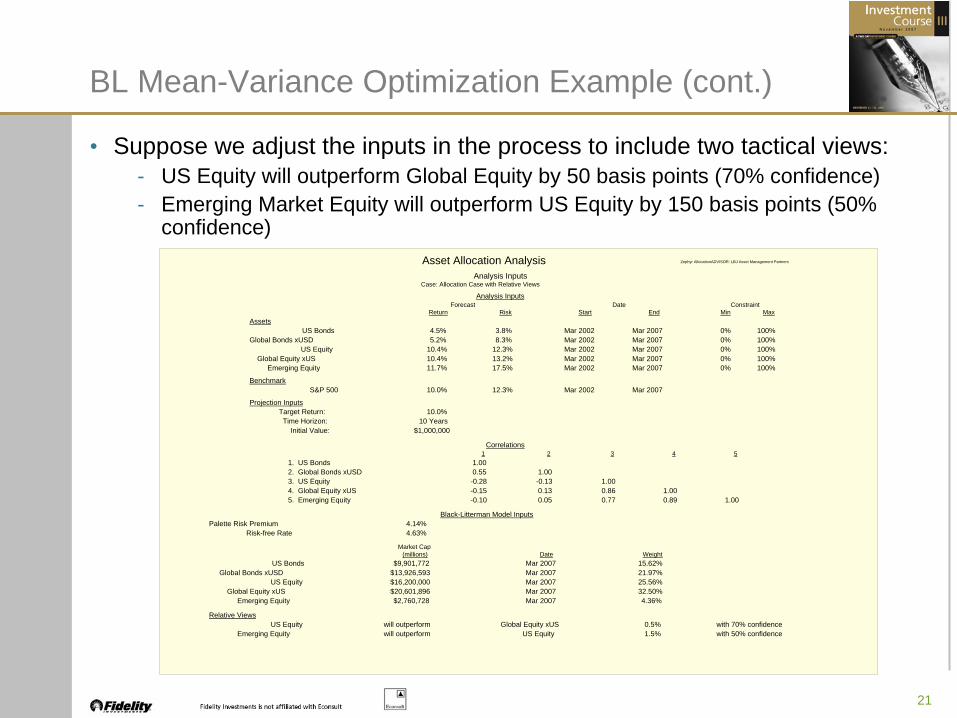
• Suppose we adjust the inputs in the process to include two tactical views:- US Equity will outperform Global Equity by 50 basis points (70% confidence)- Emerging Market Equity will outperform US Equity by 150 basis points (50%
confidence)Asset Allocation Analysis Zephyr AllocationADVISOR: LBJ Asset Management Partners
Analysis InputsCase: Allocation Case with Relative Views
Analysis InputsForecast Date Constraint
Return Risk Start End Min MaxAssets
US Bonds 4.5% 3.8% Mar 2002 Mar 2007 0% 100%Global Bonds xUSD 5.2% 8.3% Mar 2002 Mar 2007 0% 100%
US Equity 10.4% 12.3% Mar 2002 Mar 2007 0% 100%Global Equity xUS 10.4% 13.2% Mar 2002 Mar 2007 0% 100%
Emerging Equity 11.7% 17.5% Mar 2002 Mar 2007 0% 100%
BenchmarkS&P 500 10.0% 12.3% Mar 2002 Mar 2007
Projection InputsTarget Return: 10.0%Time Horizon: 10 Years
Initial Value: $1,000,000
Correlations1 2 3 4 5
1. US Bonds 1.002. Global Bonds xUSD 0.55 1.003. US Equity -0.28 -0.13 1.004. Global Equity xUS -0.15 0.13 0.86 1.005. Emerging Equity -0.10 0.05 0.77 0.89 1.00
Black-Litterman Model InputsPalette Risk Premium 4.14%
Risk-free Rate 4.63%
Market Cap(millions) Date Weight
US Bonds $9,901,772 Mar 2007 15.62%Global Bonds xUSD $13,926,593 Mar 2007 21.97%
US Equity $16,200,000 Mar 2007 25.56%Global Equity xUS $20,601,896 Mar 2007 32.50%
Emerging Equity $2,760,728 Mar 2007 4.36%
Relative ViewsUS Equity will outperform Global Equity xUS 0.5% with 70% confidence
Emerging Equity will outperform US Equity 1.5% with 50% confidence
BL Mean-Variance Optimization Example (cont.)
22
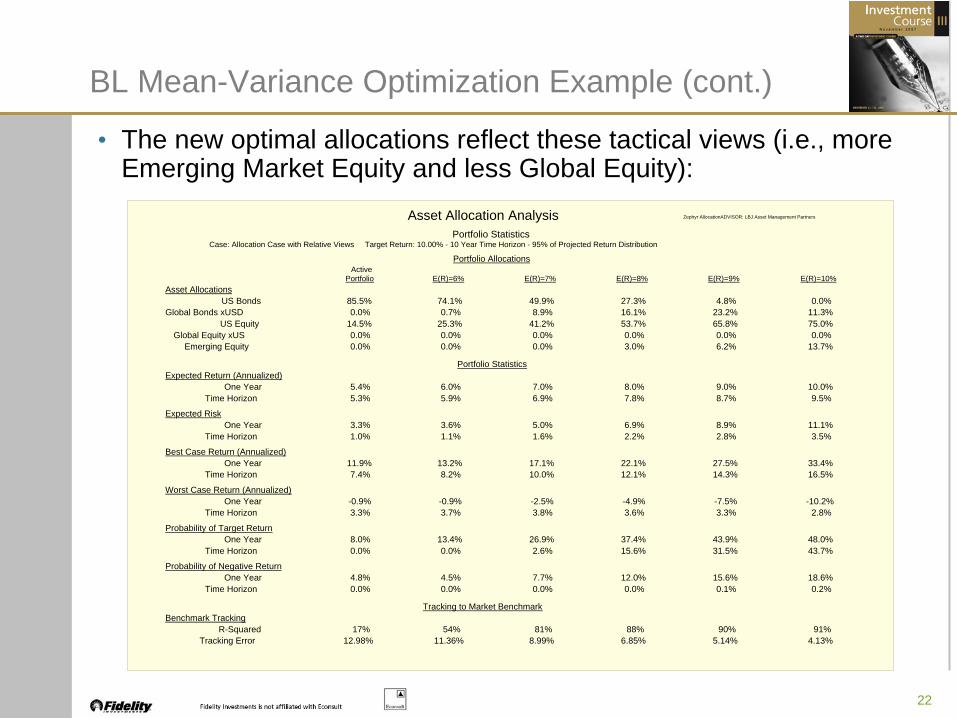
• The new optimal allocations reflect these tactical views (i.e., more Emerging Market Equity and less Global Equity):
Asset Allocation Analysis Zephyr AllocationADVISOR: LBJ Asset Management Partners
Portfolio StatisticsCase: Allocation Case with Relative Views Target Return: 10.00% - 10 Year Time Horizon - 95% of Projected Return Distribution
Portfolio AllocationsActive
Portfolio E(R)=6% E(R)=7% E(R)=8% E(R)=9% E(R)=10%Asset Allocations
US Bonds 85.5% 74.1% 49.9% 27.3% 4.8% 0.0%Global Bonds xUSD 0.0% 0.7% 8.9% 16.1% 23.2% 11.3%
US Equity 14.5% 25.3% 41.2% 53.7% 65.8% 75.0%Global Equity xUS 0.0% 0.0% 0.0% 0.0% 0.0% 0.0%
Emerging Equity 0.0% 0.0% 0.0% 3.0% 6.2% 13.7%
Portfolio StatisticsExpected Return (Annualized)
One Year 5.4% 6.0% 7.0% 8.0% 9.0% 10.0%Time Horizon 5.3% 5.9% 6.9% 7.8% 8.7% 9.5%
Expected RiskOne Year 3.3% 3.6% 5.0% 6.9% 8.9% 11.1%
Time Horizon 1.0% 1.1% 1.6% 2.2% 2.8% 3.5%
Best Case Return (Annualized)One Year 11.9% 13.2% 17.1% 22.1% 27.5% 33.4%
Time Horizon 7.4% 8.2% 10.0% 12.1% 14.3% 16.5%
Worst Case Return (Annualized)One Year -0.9% -0.9% -2.5% -4.9% -7.5% -10.2%
Time Horizon 3.3% 3.7% 3.8% 3.6% 3.3% 2.8%
Probability of Target ReturnOne Year 8.0% 13.4% 26.9% 37.4% 43.9% 48.0%
Time Horizon 0.0% 0.0% 2.6% 15.6% 31.5% 43.7%
Probability of Negative ReturnOne Year 4.8% 4.5% 7.7% 12.0% 15.6% 18.6%
Time Horizon 0.0% 0.0% 0.0% 0.0% 0.1% 0.2%
Tracking to Market BenchmarkBenchmark Tracking
R-Squared 17% 54% 81% 88% 90% 91%Tracking Error 12.98% 11.36% 8.99% 6.85% 5.14% 4.13%
BL Mean-Variance Optimization Example (cont.)
23
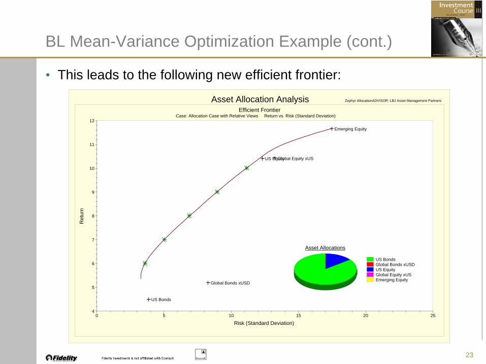
• This leads to the following new efficient frontier:
Asset Allocation Analysis Zephyr AllocationADVISOR: LBJ Asset Management Partners
Efficient FrontierCase: Allocation Case with Relative Views Return vs. Risk (Standard Deviation)
0 5 10 15 20 254
5
6
7
8
9
10
11
12
Risk (Standard Deviation)
Ret
urn
US BondsGlobal Bonds xUSDUS EquityGlobal Equity xUSEmerging Equity
Asset Allocations
US Bonds
Global Bonds xUSD
US EquityGlobal Equity xUS
Emerging Equity
BL Mean-Variance Optimization Example (cont.)
24
Optimal Portfolio Formation With Historical Returns: Examples
• Suppose we have monthly return data for the three recent years on the following six asset classes:
Chilean Stocks (IPSA Index)Chilean Bonds (LVAG & LVAC Indexes)Chilean Cash (LVAM Index)U.S. Stocks (S&P 500 Index)U.S. Bonds (SBBIG Index)Multi-Strategy Hedge Funds (CSFB/Tremont Index)
• Assume also that the non-CLP denominated asset classes can be perfectly and costlessly hedged in full if the investor so desires
25
Optimal Portfolio Formation With Historical Returns: Examples (cont.)
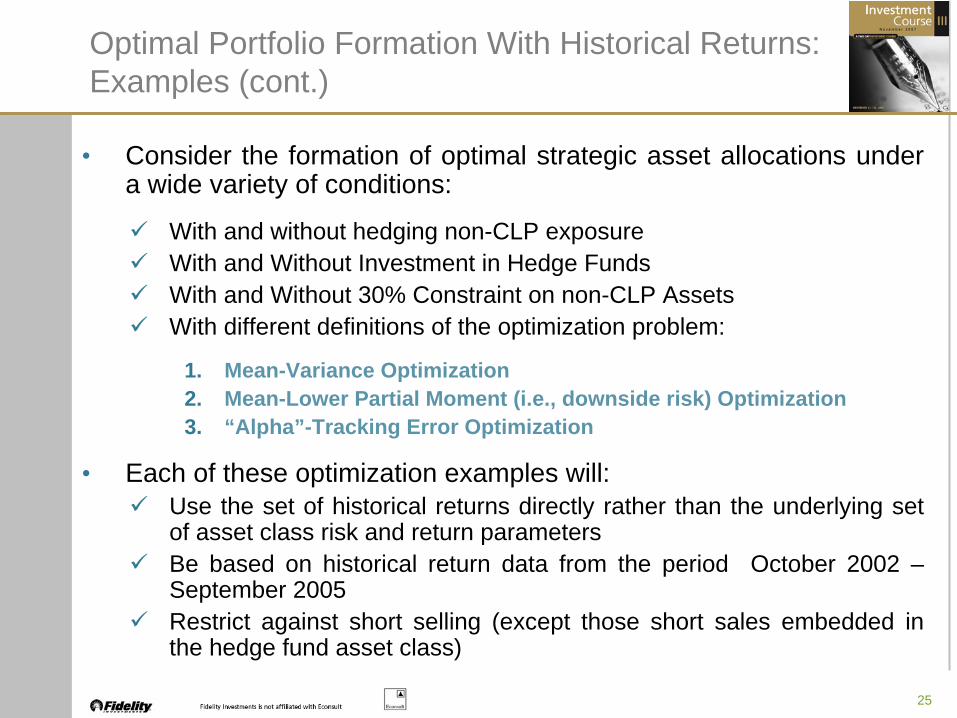
• Consider the formation of optimal strategic asset allocations under a wide variety of conditions:
With and without hedging non-CLP exposureWith and Without Investment in Hedge FundsWith and Without 30% Constraint on non-CLP AssetsWith different definitions of the optimization problem:
1. Mean-Variance Optimization2. Mean-Lower Partial Moment (i.e., downside risk) Optimization3. “Alpha”-Tracking Error Optimization
• Each of these optimization examples will:Use the set of historical returns directly rather than the underlying set of asset class risk and return parameters Be based on historical return data from the period October 2002 –September 2005Restrict against short selling (except those short sales embedded in the hedge fund asset class)

26
1. Mean-Variance Optimization: Non-CLP Assets 100% Unhedged

27
Unconstrained Efficient Frontier: 100% Unhedged
E(R) σp Relative σp Wcs Wcb Wcc Wuss Wusb Whf
5.00% 1.13% 1.000 7.95% 6.18% 85.87% 0.00% 0.00% 0.00%
6.00% 1.65% 1.000 11.80% 9.15% 79.05% 0.00% 0.00% 0.00%
7.00% 2.18% 1.000 15.65% 12.12% 72.23% 0.00% 0.00% 0.00%
8.00% 2.71% 1.000 19.49% 15.09% 65.42% 0.00% 0.00% 0.00%
9.00% 3.24% 1.000 23.34% 18.06% 58.60% 0.00% 0.00% 0.00%
10.00% 3.77% 1.000 27.19% 21.03% 51.78% 0.00% 0.00% 0.00%
11.00% 4.30% 1.000 31.03% 24.00% 44.96% 0.00% 0.00% 0.00%
12.00% 4.83% 1.000 34.88% 26.97% 38.15% 0.00% 0.00% 0.00%
13.00% 5.36% 1.000 38.73% 29.94% 31.33% 0.00% 0.00% 0.00%
14.00% 5.90% 1.000 42.57% 32.92% 24.51% 0.00% 0.00% 0.00%
28
One Consequence of the Unhedged M-V Efficient Frontier
• Notice that because of the strengthening CLP/USD exchange rate over the October 2002 – September 2005 period, the optimal allocation for any expected return goal did not include any exposure to non-CLP asset classes
• This “unhedged foreign investment” efficient frontier is equivalent to the efficient frontier that would have resulted from a “domestic investment only” constraint.

29
Mean-Variance Optimization: Non-CLP Assets 100% Hedged
30
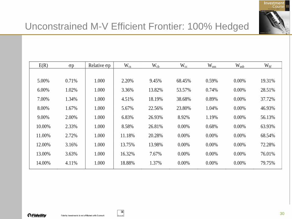
Unconstrained M-V Efficient Frontier: 100% Hedged
E(R) σp Relative σp Wcs Wcb Wcc Wuss Wusb Whf
5.00% 0.71% 1.000 2.20% 9.45% 68.45% 0.59% 0.00% 19.31%
6.00% 1.02% 1.000 3.36% 13.82% 53.57% 0.74% 0.00% 28.51%
7.00% 1.34% 1.000 4.51% 18.19% 38.68% 0.89% 0.00% 37.72%
8.00% 1.67% 1.000 5.67% 22.56% 23.80% 1.04% 0.00% 46.93%
9.00% 2.00% 1.000 6.83% 26.93% 8.92% 1.19% 0.00% 56.13%
10.00% 2.33% 1.000 8.58% 26.81% 0.00% 0.68% 0.00% 63.93%
11.00% 2.72% 1.000 11.18% 20.28% 0.00% 0.00% 0.00% 68.54%
12.00% 3.16% 1.000 13.75% 13.98% 0.00% 0.00% 0.00% 72.28%
13.00% 3.63% 1.000 16.32% 7.67% 0.00% 0.00% 0.00% 76.01%
14.00% 4.11% 1.000 18.88% 1.37% 0.00% 0.00% 0.00% 79.75%
31
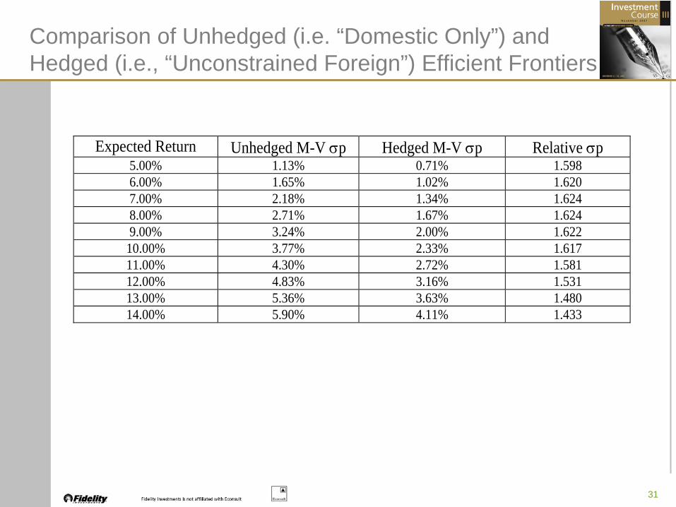
Comparison of Unhedged (i.e. “Domestic Only”) and Hedged (i.e., “Unconstrained Foreign”) Efficient Frontiers
Expected Return Unhedged M-V σp Hedged M-V σp Relative σp 5.00% 1.13% 0.71% 1.598 6.00% 1.65% 1.02% 1.620 7.00% 2.18% 1.34% 1.624 8.00% 2.71% 1.67% 1.624 9.00% 3.24% 2.00% 1.622
10.00% 3.77% 2.33% 1.617 11.00% 4.30% 2.72% 1.581 12.00% 4.83% 3.16% 1.531 13.00% 5.36% 3.63% 1.480 14.00% 5.90% 4.11% 1.433
32
A Related Question About Foreign Diversification
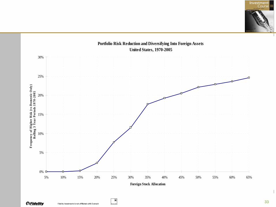
• What allocation to foreign assets in a domestic investment portfolio leads to a reduction in the overall level of risk?
• Van Harlow of Fidelity Investments performed the following analysis:
Consider a benchmark portfolio containing a 100% allocation to U.S. equitiesDiversify the benchmark portfolio by adding a foreign equity allocation in successive 5% incrementsCalculate standard deviations for benchmark and diversified portfolios using monthly return data over rolling three-year holding periods during 1970-2005For each foreign allocation proportion, calculate the percentage of rolling three-year holding periods that resulted in a risk level for the diversified portfolio that was higher than the domestic benchmark
33
Portfolio Risk Reduction and Diversifying Into Foreign AssetsUnited States, 1970-2005
0%
5%
10%
15%
20%
25%
30%
5% 10% 15% 20% 25% 30% 35% 40% 45% 50% 55% 60% 65%
Foreign Stock Allocation
Freq
uenc
y of
Hig
her
Risk
(vs D
omes
tic O
nly)
Rol
ling
3 Y
ear
Peri
ods 1
970-
2005
34
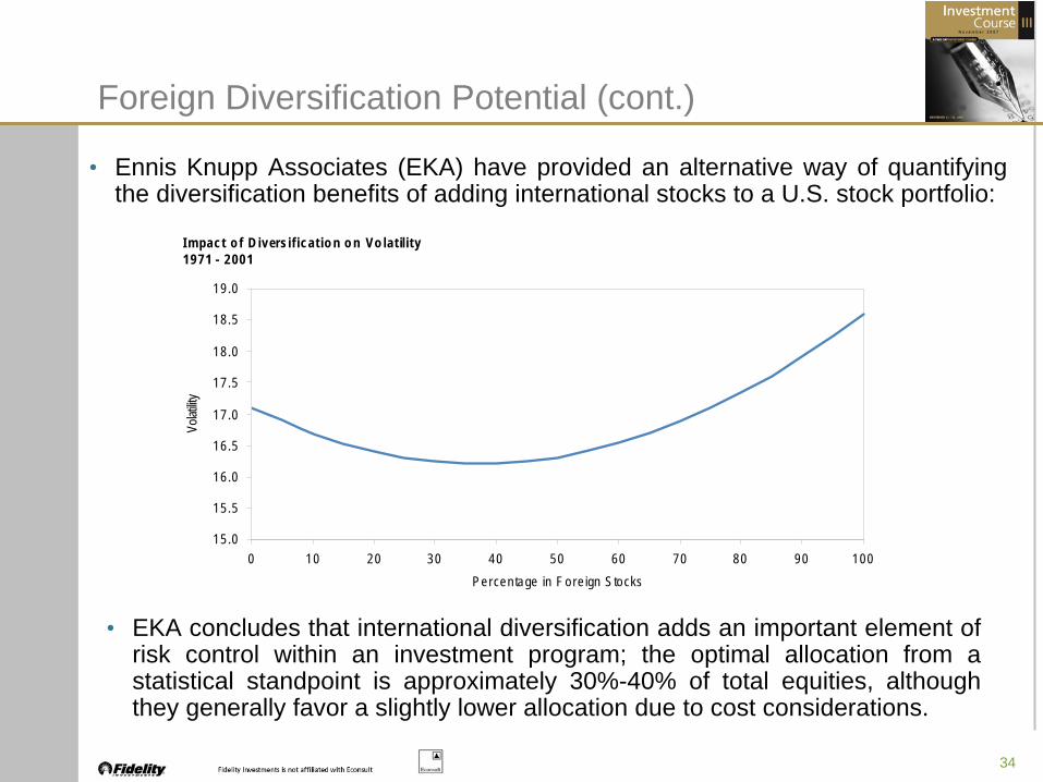
Foreign Diversification Potential (cont.)
• Ennis Knupp Associates (EKA) have provided an alternative way of quantifying the diversification benefits of adding international stocks to a U.S. stock portfolio:
• EKA concludes that international diversification adds an important element of risk control within an investment program; the optimal allocation from a statistical standpoint is approximately 30%-40% of total equities, although they generally favor a slightly lower allocation due to cost considerations.
I mpact o f D ivers if icat io n o n Vo lat ility1971 - 2001
15 .0
15 .5
16 .0
16 .5
17 .0
17 .5
18 .0
18 .5
19 .0
0 10 20 30 40 50 60 70 80 90 100Percen tage in F o re ign S tocks
Volat
ility

35
Foreign Diversification Potential: One Caveat
• During recent periods, it appears as though the correlations between U.S. and non-U.S. markets are increasing, reducing the diversification benefits of non-U.S. markets.
• While this is true, the fact that these markets are less than perfectly correlated means that there is still a diversification benefit afforded to investors who allocate a portion of their assets overseas.
Rolling 3-Year CorrelationsU.S. and Non-U.S. Stocks1971-2001
0.0
0.10.2
0.30.4
0.5
0.60.70.8
0.9
1.0
1974
1975
1977
1978
1979
1980
1982
1983
1984
1985
1987
1988
1989
1990
1992
1993
1994
1995
1997
1998
1999
2000
2002
36
More on Mean-Variance Optimization: The Cost of Adding Additional Constraints
• Start with the following base case:
Six asset classes: Three Chilean, Three Foreign (Including Hedge Funds)No Short Sales100% Hedged Foreign InvestmentsNo Constraint on Total Foreign InvestmentNo Constraint on Hedge Fund Investment
• Consider the addition of two more constraints:
30% Limit on Foreign Asset ClassesNo Hedge Funds

37
Additional Constraints: 30% Foreign Investment
E(R) σp Relative σp Wcs Wcb Wcc Wuss Wusb Whf
5.00% 0.71% 1.000 2.20% 9.45% 68.45% 0.59% 0.00% 19.31%
6.00% 1.02% 1.000 3.36% 13.82% 53.57% 0.74% 0.00% 28.51%
7.00% 1.40% 1.040 7.00% 16.77% 46.22% 0.63% 0.00% 29.37%
8.00% 1.85% 1.109 10.87% 19.60% 39.53% 0.50% 0.00% 29.50%
9.00% 2.34% 1.171 14.73% 22.43% 32.84% 0.37% 0.00% 29.63%
10.00% 2.84% 1.218 18.59% 25.25% 26.15% 0.24% 0.00% 29.76%
11.00% 3.35% 1.233 22.45% 27.97% 19.58% 0.10% 0.00% 29.90%
12.00% 3.87% 1.226 26.31% 30.93% 12.76% 0.00% 0.00% 30.00%
13.00% 4.39% 1.212 30.16% 33.90% 5.94% 0.00% 0.00% 30.00%
14.00% 4.92% 1.195 33.99% 36.01% 0.00% 0.00% 0.00% 30.00%
38
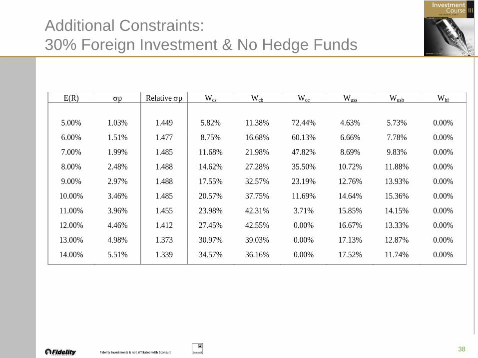
Additional Constraints: 30% Foreign Investment & No Hedge Funds
E(R) σp Relative σp Wcs Wcb Wcc Wuss Wusb Whf
5.00% 1.03% 1.449 5.82% 11.38% 72.44% 4.63% 5.73% 0.00%
6.00% 1.51% 1.477 8.75% 16.68% 60.13% 6.66% 7.78% 0.00%
7.00% 1.99% 1.485 11.68% 21.98% 47.82% 8.69% 9.83% 0.00%
8.00% 2.48% 1.488 14.62% 27.28% 35.50% 10.72% 11.88% 0.00%
9.00% 2.97% 1.488 17.55% 32.57% 23.19% 12.76% 13.93% 0.00%
10.00% 3.46% 1.485 20.57% 37.75% 11.69% 14.64% 15.36% 0.00%
11.00% 3.96% 1.455 23.98% 42.31% 3.71% 15.85% 14.15% 0.00%
12.00% 4.46% 1.412 27.45% 42.55% 0.00% 16.67% 13.33% 0.00%
13.00% 4.98% 1.373 30.97% 39.03% 0.00% 17.13% 12.87% 0.00%
14.00% 5.51% 1.339 34.57% 36.16% 0.00% 17.52% 11.74% 0.00%
39
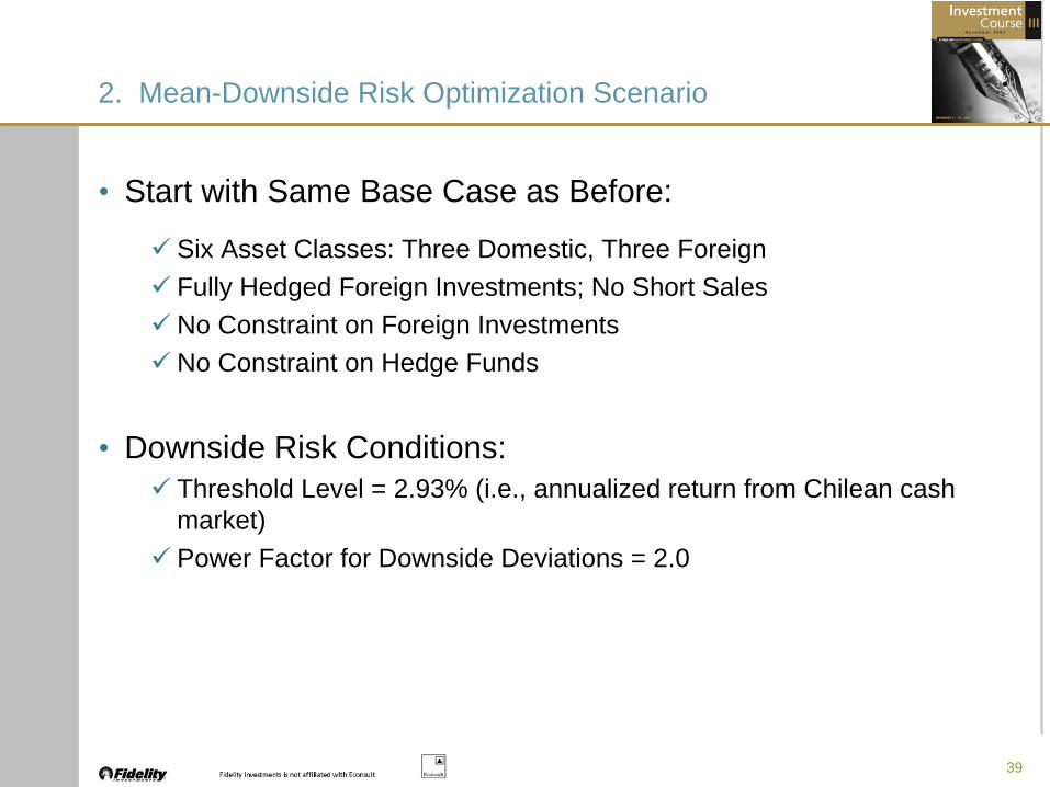
• Start with Same Base Case as Before:
Six Asset Classes: Three Domestic, Three ForeignFully Hedged Foreign Investments; No Short SalesNo Constraint on Foreign InvestmentsNo Constraint on Hedge Funds
• Downside Risk Conditions:Threshold Level = 2.93% (i.e., annualized return from Chilean cash market)Power Factor for Downside Deviations = 2.0
2. Mean-Downside Risk Optimization Scenario
40
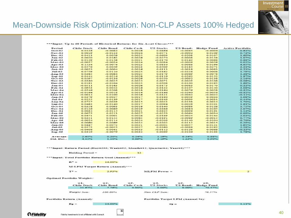
Mean-Downside Risk Optimization: Non-CLP Assets 100% Hedged
41
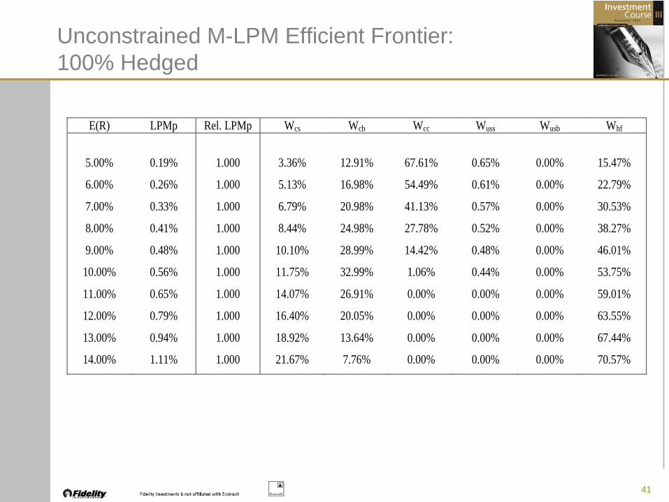
Unconstrained M-LPM Efficient Frontier: 100% Hedged
E(R) LPMp Rel. LPMp Wcs Wcb Wcc Wuss Wusb Whf
5.00% 0.19% 1.000 3.36% 12.91% 67.61% 0.65% 0.00% 15.47%
6.00% 0.26% 1.000 5.13% 16.98% 54.49% 0.61% 0.00% 22.79%
7.00% 0.33% 1.000 6.79% 20.98% 41.13% 0.57% 0.00% 30.53%
8.00% 0.41% 1.000 8.44% 24.98% 27.78% 0.52% 0.00% 38.27%
9.00% 0.48% 1.000 10.10% 28.99% 14.42% 0.48% 0.00% 46.01%
10.00% 0.56% 1.000 11.75% 32.99% 1.06% 0.44% 0.00% 53.75%
11.00% 0.65% 1.000 14.07% 26.91% 0.00% 0.00% 0.00% 59.01%
12.00% 0.79% 1.000 16.40% 20.05% 0.00% 0.00% 0.00% 63.55%
13.00% 0.94% 1.000 18.92% 13.64% 0.00% 0.00% 0.00% 67.44%
14.00% 1.11% 1.000 21.67% 7.76% 0.00% 0.00% 0.00% 70.57%

42
Additional Constraints: 30% Foreign Investment
E(R) LPMp Rel. LPMp Wcs Wcb Wcc Wuss Wusb Whf
5.00% 0.19% 1.000 3.36% 12.91% 67.61% 0.65% 0.00% 15.47%
6.00% 0.26% 1.000 5.13% 16.98% 54.49% 0.61% 0.00% 22.79%
7.00% 0.33% 1.002 7.12% 20.75% 42.13% 0.42% 0.00% 29.58%
8.00% 0.45% 1.098 11.04% 24.30% 34.66% 0.00% 0.00% 30.00%
9.00% 0.59% 1.233 14.90% 27.81% 27.29% 0.00% 0.00% 30.00%
10.00% 0.76% 1.361 18.79% 32.63% 18.58% 0.00% 0.00% 30.00%
11.00% 0.93% 1.432 22.68% 37.57% 9.75% 0.00% 0.00% 30.00%
12.00% 1.12% 1.422 26.46% 43.47% 0.07% 0.89% 0.00% 29.11%
13.00% 1.32% 1.401 30.29% 39.71% 0.00% 0.00% 0.00% 30.00%
14.00% 1.53% 1.384 33.99% 36.01% 0.00% 0.00% 0.00% 30.00%
43
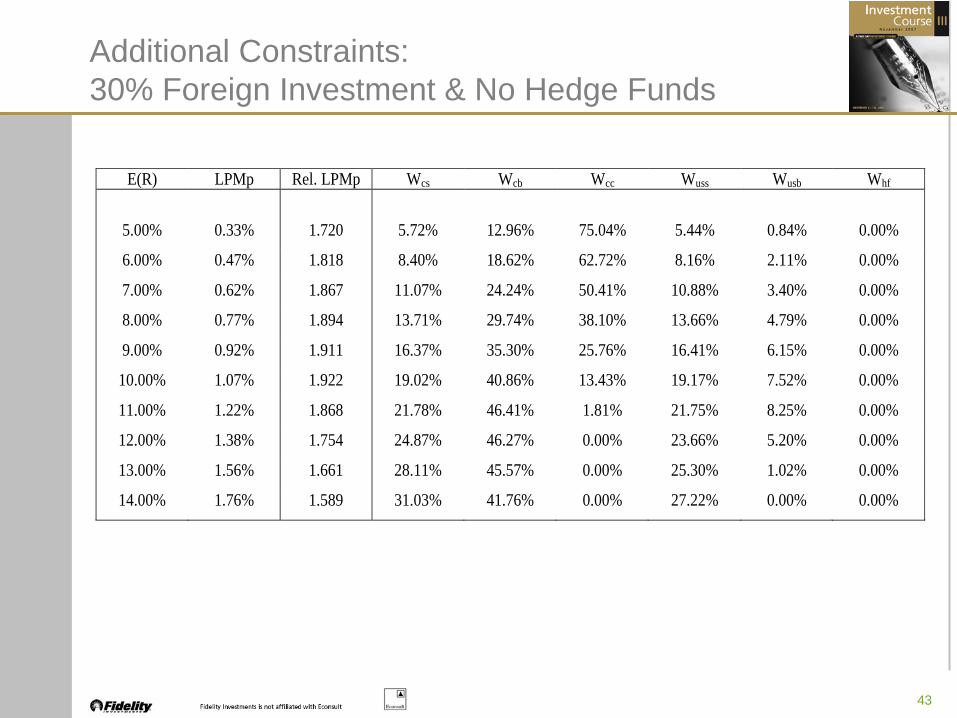
Additional Constraints: 30% Foreign Investment & No Hedge Funds
E(R) LPMp Rel. LPMp Wcs Wcb Wcc Wuss Wusb Whf
5.00% 0.33% 1.720 5.72% 12.96% 75.04% 5.44% 0.84% 0.00%
6.00% 0.47% 1.818 8.40% 18.62% 62.72% 8.16% 2.11% 0.00%
7.00% 0.62% 1.867 11.07% 24.24% 50.41% 10.88% 3.40% 0.00%
8.00% 0.77% 1.894 13.71% 29.74% 38.10% 13.66% 4.79% 0.00%
9.00% 0.92% 1.911 16.37% 35.30% 25.76% 16.41% 6.15% 0.00%
10.00% 1.07% 1.922 19.02% 40.86% 13.43% 19.17% 7.52% 0.00%
11.00% 1.22% 1.868 21.78% 46.41% 1.81% 21.75% 8.25% 0.00%
12.00% 1.38% 1.754 24.87% 46.27% 0.00% 23.66% 5.20% 0.00%
13.00% 1.56% 1.661 28.11% 45.57% 0.00% 25.30% 1.02% 0.00%
14.00% 1.76% 1.589 31.03% 41.76% 0.00% 27.22% 0.00% 0.00%
44
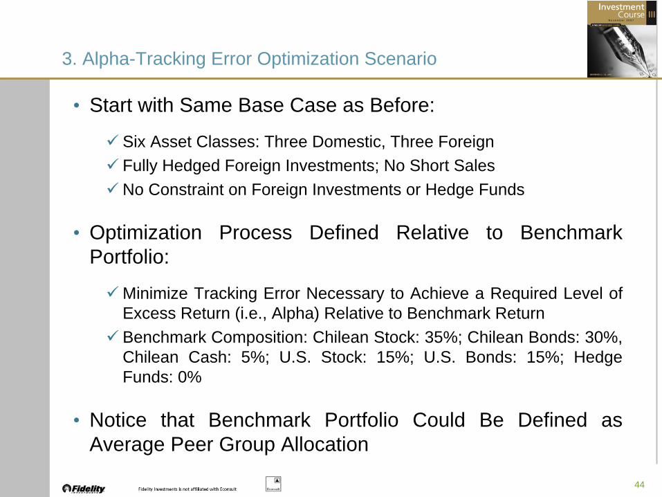
3. Alpha-Tracking Error Optimization Scenario
• Start with Same Base Case as Before:
Six Asset Classes: Three Domestic, Three ForeignFully Hedged Foreign Investments; No Short SalesNo Constraint on Foreign Investments or Hedge Funds
• Optimization Process Defined Relative to Benchmark Portfolio:
Minimize Tracking Error Necessary to Achieve a Required Level ofExcess Return (i.e., Alpha) Relative to Benchmark ReturnBenchmark Composition: Chilean Stock: 35%; Chilean Bonds: 30%, Chilean Cash: 5%; U.S. Stock: 15%; U.S. Bonds: 15%; Hedge Funds: 0%
• Notice that Benchmark Portfolio Could Be Defined as Average Peer Group Allocation
45
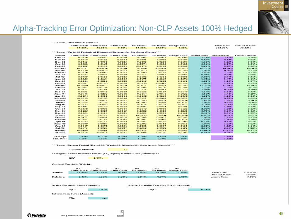
Alpha-Tracking Error Optimization: Non-CLP Assets 100% Hedged

46
α TE Relative TE Wcs Wcb Wcc Wuss Wusb Whf
0.20% 0.07% 1.000 35.23% 30.87% 2.16% 15.01% 14.83% 1.90%
0.40% 0.13% 1.000 35.51% 31.35% 0.00% 14.94% 14.46% 3.74%
0.60% 0.22% 1.000 35.96% 30.57% 0.00% 14.60% 13.46% 5.41%
0.80% 0.31% 1.000 36.41% 29.79% 0.00% 14.26% 12.45% 7.08%
1.00% 0.40% 1.000 36.85% 29.02% 0.00% 13.93% 11.45% 8.75%
1.20% 0.49% 1.000 37.30% 28.24% 0.00% 13.59% 10.44% 10.42%
1.40% 0.59% 1.000 37.75% 27.47% 0.00% 13.25% 9.44% 12.09%
1.60% 0.68% 1.000 38.19% 26.69% 0.00% 12.92% 8.43% 13.76%
1.80% 0.78% 1.000 38.64% 25.92% 0.00% 12.58% 7.43% 15.43%
2.00% 0.87% 1.000 39.09% 25.14% 0.00% 12.25% 6.42% 17.10%
Unconstrained α-TE Efficient Frontier: 100% Hedged
47
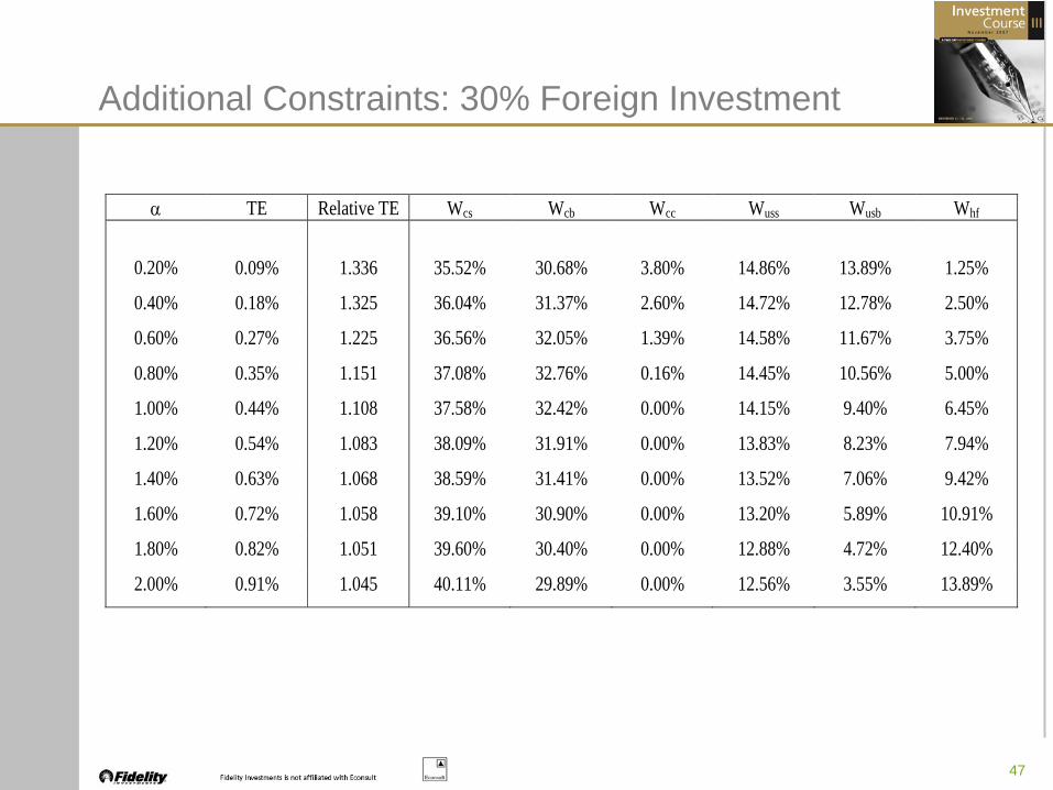
Additional Constraints: 30% Foreign Investment
α TE Relative TE Wcs Wcb Wcc Wuss Wusb Whf
0.20% 0.09% 1.336 35.52% 30.68% 3.80% 14.86% 13.89% 1.25%
0.40% 0.18% 1.325 36.04% 31.37% 2.60% 14.72% 12.78% 2.50%
0.60% 0.27% 1.225 36.56% 32.05% 1.39% 14.58% 11.67% 3.75%
0.80% 0.35% 1.151 37.08% 32.76% 0.16% 14.45% 10.56% 5.00%
1.00% 0.44% 1.108 37.58% 32.42% 0.00% 14.15% 9.40% 6.45%
1.20% 0.54% 1.083 38.09% 31.91% 0.00% 13.83% 8.23% 7.94%
1.40% 0.63% 1.068 38.59% 31.41% 0.00% 13.52% 7.06% 9.42%
1.60% 0.72% 1.058 39.10% 30.90% 0.00% 13.20% 5.89% 10.91%
1.80% 0.82% 1.051 39.60% 30.40% 0.00% 12.88% 4.72% 12.40%
2.00% 0.91% 1.045 40.11% 29.89% 0.00% 12.56% 3.55% 13.89%

48
Additional Constraints: 30% Foreign Investment & No Hedge Funds
α TE Relative TE Wcs Wcb Wcc Wuss Wusb Whf
0.20% 0.10% 1.558 35.68% 30.92% 3.40% 15.24% 14.76% 0.00%
0.40% 0.21% 1.546 36.36% 31.83% 1.81% 15.49% 14.51% 0.00%
0.60% 0.31% 1.430 37.05% 32.77% 0.19% 15.73% 14.27% 0.00%
0.80% 0.42% 1.353 37.75% 32.25% 0.00% 15.84% 14.16% 0.00%
1.00% 0.53% 1.314 38.45% 31.55% 0.00% 15.94% 14.06% 0.00%
1.20% 0.64% 1.292 39.16% 30.84% 0.00% 16.03% 13.97% 0.00%
1.40% 0.75% 1.278 39.86% 30.14% 0.00% 16.12% 13.88% 0.00%
1.60% 0.87% 1.268 40.60% 29.70% 0.00% 16.19% 13.51% 0.00%
1.80% 0.98% 1.261 41.34% 29.29% 0.00% 16.25% 13.13% 0.00%
2.00% 1.10% 1.255 42.07% 28.88% 0.00% 16.31% 12.74% 0.00%
49
The Portfolio Optimization Process: Some Summary Comments
• The introduction of the portfolio optimization process was an important step in the development of what is now considered to be modern finance theory. These techniques have been widely used in practice for more than fifty years.
• Portfolio optimization is an effective tool for establishing the strategic asset allocation policy for a investment portfolio. It is most likely to be usefully employed at the asset class level rather than at the individual security level.
• There are two critical implementation decisions that the investor must make:
The nature of the risk-return problem:Mean-Variance, Mean-Downside Risk, Excess Return-Tracking Error
Estimates of the required inputs :Expected returns, asset class risk, correlations
• Portfolio optimization routines can be adapted to include a variety of restrictions on the investment process (e.g., no short sales, limits on foreign investing).
The cost of such investment constraints can be viewed in terms of the incremental volatility that the investor is required to bear to obtain the same expected outcome