EDHEC RISK AND ASSET MANAGEMENT RESEARCH CENTEREdhec -1090 route des crêtes - 06560 Valbonne - Tel. +33 (0)4 92 96 89 50 - Fax. +33 (0)4 92 96 93 22

Email: research@edhec-risk.com – Web: www.edhec-risk.com

Portable Alpha and Portable Beta Strategies in the Euro Zone

Implementing Active Asset Allocation Decisions using EquityIndex Options and Futures

October 30th, 2003

Noël Amenc, PhDEDHEC Graduate School of Business

Philippe MalaiseEDHEC Graduate School of Business

Lionel Martellini, PhDEDHEC Graduate School of Business

Daphne Sfeir, PhDEDHEC Risk and Asset Management Research Center

This research is sponsored by Eurex

Abstract:

While stock picking strategies are in principle meant to exploit evidence of predictability in individual stockspecific risk, most equity managers, as a result of their bottom-up security selection decisions, often endup making discretionary, and most of the time unintended, bets on market, sector and style returns asmuch as they make bets on individual stock returns. In this paper, we show how portfolio managers in theEuro-zone can benefit from using derivatives markets to actively manage their asset allocation decisionsin a systematic manner. Using a robust econometric process based on a non-linear multi-factor thick andrecursive modeling approach, we report statistically and economically significant evidence of predictabilityin Dow Jones EURO STOXX 50 excess return. These econometric forecasts can be turned into activeportfolio decisions and implemented via Eurex index futures to generate active asset allocation portablealpha benefits. We also show that adding active sector rotation decisions to asset allocation decisionsallows one to significantly lower the portfolio volatility as a result of the benefits of bet diversification: Wefinally explain how active portfolio managers can benefit from using suitably designed Eurex optionstrategies as portable beta vehicles. In particular, option portfolios can be used to enhance theperformance of tactical asset allocation programs by consistently adding value during the periods of lowvolatility when timing strategies are known to perform rather poorly. The benefits of active asset allocationdecisions reported in this paper originate from the combination of a robust econometric and portfolioprocess on the one hand, and an efficient trading of low cost investible products such as Eurex indexfutures and options on the other hand. This strongly suggests that most long-short managers could use asimilar methodology to enhance the performance of their portfolios without having to rely on the allegedsuperior performance of any specific predictive model.

Noël Amenc, PhD, is a professor of finance at Edhec where he heads the Risk and Asset Management ResearchCenter. He is also head of research at Misys Asset Management Systems, a company that develops softwaresolutions for portfolio analysis and performance evaluation. He is an Associate Editor of the Journal of AlternativeInvestments, and has co-authored a book on Portfolio Analysis and Performance Measurement.

Philippe Malaise is a professor of finance at Edhec. He also heads the tactical asset allocation program at EDHECRisk and Asset Management Research Center. His expertise is in optimal portfolio selection. Philippe has served as aconsultant in the domain of active asset allocation for various international institutions.

Lionel Martellini, PhD, is a professor of finance at Edhec and the scientific director of the EDHEC Risk and AssetManagement Research Center. He conducts active research in alternative investment strategies, quantitative assetmanagement and derivatives valuation, and has served as a consultant for various international institutions on thesetopics. He is a member of the Editorial Board of the Journal of Alternative Investments, as well as the Journal of BondTrading and Management. He has co-authored two reference textbooks on Fixed-Income Securities with John Wiley.

Daphne Sfeir, PhD, is a research engineer at EDHEC Risk and Asset Management Research Center. Herbackground is in astrophysics and aerospace engineering, and her expertise in econometric models in finance.Daphne has served as a consultant in the domain of active asset allocation and portfolio performance evaluation forvarious international institutions.

Edhec is one of the top five business schools in France owing to the high quality of its academic staff (90 permanentlecturers from France and abroad) and its privileged relationship with professionals that the school has beendeveloping since its establishment in 1906. Edhec Business School has decided to draw on its extensive knowledgeof the professional environment and has therefore concentrated its research on themes that satisfy the needs ofprofessionals.Edhec pursues an active research policy in the field of finance. Its “Risk and Asset Management ResearchCenter” carries out numerous research programs in the areas of asset allocation and risk management in both thetraditional and alternative investment universes.

Copyright © 2003 Edhec

1

While stock picking strategies are in principle meant to exploit evidence of predictability in individual

stock specific risk, equity managers, as a result of their bottom-up security selection decisions, often

end up making discretionary, and most of the time unintended, bets on market, sector and style

returns as much as they make bets on individual stock returns.i These unintended bets are unfortunate

as they can have a dramatic, positive or negative, impact on the portfolio return, and their presence

introduces an undesirable element of luck in the performance generating process.

Consider for example the case of long/short equity managers. The vast majority favor stock picking as

a way to generate abnormal return. Long/short managers do not generally actively manage their

market exposure, and most of them end up having a net long bias. This can be seen for example from

the correlation of HFR Equity Hedge (a prominent index for long/short hedge fund managers) with the

S&P500, which turns out to be equal to 0.63 based on monthly data over the period 1990-2000. This

is due to the fact that these managers, most of them being originally long-only mutual fund managers,

typically feel more comfortable at detecting undervalued stocks than overvalued stocks. This long bias,

which is not the result of an active bet on a bullish market trend but merely the result of a lack of

perceived opportunities on the short selling side, has undoubtedly explained a large fraction of the

performance of these managers in the extended bull market periods of the 90s. On the other hand, it

has very significantly hurt their performance in the past few years of market downturns. Similarly,

long/short managers, even those who target market neutrality, have unintended time-varying residual

exposure to a variety of sectors or investment styles (growth or value, small cap or large cap) resulting

from their bottom-up stock picking decisions. Since very few managers are both market and factor

neutral, it is not obvious to extract from their performance anything but a very noisy signal on their

pure stock picking ability.

In this paper, we show how long/short managers in the Euro zone can use derivatives markets to help

actively manage their asset and sector allocation decisions in a systematic manner so as to enhance

the performance of their portfolio. It should be emphasized at this point that the benefits of active asset

allocation decisions that we present in this experiment are not based on the use of any specific

econometric model with unusually superior predictive power. In the interest of underlining a

methodology that could be used by a set of long-short managers endowed with reasonable

econometric skills, we use in this paper an econometric approach, known as “thick modeling”, which is

based on a process that consists of selecting at each date a “council” of models to make predictions,

as opposed to using a single model. In other words, the benefits of active asset allocation decisions

reported in this paper originate from the combination of a robust econometric and portfolio process on

the one hand, and an efficient trading of low cost investible products such as Eurex index futures and

options on the other hand. This strongly suggests that most long-short managers could use a similar

methodology to enhance the performance of their portfolios without having to rely on the alleged

superior performance of any specific predictive model.

2

Active management of asset allocation decision actually comes in two forms. The first possible form of

an active asset allocation strategy involves adding market and/or sector timing alpha benefits to

original stock picking based active decisions. Long/short managers can also choose to use market,

sector or style timing as an alternative way to generate alpha in the absence of confidence in their

ability to generate consistent performance through stock picking. In this paper, we show how to form a

pure overlay portfolio that is designed to capture excess return through tactical asset and factor

allocation decisions on the European markets, using active management of betas to generate

(portable) alphas. We focus on pure active allocation decisions implemented through trading in index

derivatives markets so as to study the performance of an overlay that is not impacted by stock picking

decisions, which should remain the sole focus of attention from bottom-up managers.

The second possible form of an active asset allocation strategy involves implementing an option-

based portfolio strategy, of which the sole objective is to decrease asset allocation risk in the portfolio.

In particular, options on equity indices can be used to truncate return distributions with an aim at

eliminating the few worst (and best) outliers generated from managers’ forecast errors. In this paper,

we show how suitably designed option strategies can be used to enhance the performance of an

active asset allocation strategy, the objective being to design a program which would consistently add

value during the periods of calm markets, which are typically not favorable to timing strategies. In

recent years, the core-satellite portfolio approach has become increasingly popular among investors

who attempt to add portable alpha benefits to their portfolio without modifying their passive exposure

to a reference index. In the section detailing the second possible form of an active asset allocation

strategy, we look at it from a different perspective. More specifically, we explain how active portfolio

managers can benefit from using suitably packaged derivatives satellite portfolios as portable beta

vehicles.

This paper is organized as follows. In a first section, we present the case for tactical asset allocation

(TAA) decisions. In a second section, we present some evidence of predictability in Euro equity

markets. In a third section, we show how this predictability can be exploited in a systematic way to

generate superior performance through dynamic trading in index futures. In a fourth section, we argue

that long/short managers can also use options on equity indices to implement truncated return

strategies that aim at enhancing the performance and/or at reducing the risk of a TAA program. A fifth

section extends the analysis to sector rotation decisions, while concluding remarks can be found in a

last section.

THE CASE FOR TACTICAL ASSET ALLOCATION DECISIONS

It is well known that derivative products can be used by long/short managers in all sorts of ways to

improve the risk-return profile of their portfolio. In particular index futures can be used for hedging

purposes by long/short managers who specialize in stock picking and have no views on market trends,

3

and therefore want to hedge away their residual market exposure. Hedging market risk means setting

the beta of the long/short portfolio equal to zero. While this is desirable for a stock picker who has no

view on the market direction, this may not be optimal from an active portfolio management standpoint,

as it does not take into account useful conditioning information.

There is actually now a consensus in empirical finance that expected asset returns, and also variances

and covariances, are, to some extent, predictable based on conditioning information (see for example

Keim and Stambaugh (1986), Campbell (1987), or Ferson and Harvey (1991)). In this section, we

show how these insights can be exploited by long/short managers to improve existing policies based

upon unconditional estimates.

Tactical Asset Allocation broadly refers to active strategies that seek to enhance portfolio performance

by opportunistically shifting the asset mix in a portfolio in response to the changing patterns of return

and risk. Practitioners started to engage in tactical asset allocation strategies as early as the 1970s.

The exact amount of investment currently engaged in tactical asset allocation is not clear, but it is

certainly growing very rapidly. For example, Philip, Rogers and Capaldi (1996) estimated that around

$48 billion was allocated to domestic TAA in 1994, while Lee (2000) estimates that more than $100

billion was dedicated to domestic TAA at the end of 1999.

TAA can be regarded as a 3 steps process:

• Step 1: forecast asset returns by asset classes

• Step 2: build portfolios based on forecasts (i.e., turn signals into bets)

• Step 3: conduct out-of-sample performance tests

Forecast Asset Returns by Asset Class

One first needs to distinguish between forecast-based TAA and fact-based TAA. The former approach

consists in forecasting returns by first forecasting the values of economic variables (scenarios on the

contemporaneous variables). The latter approach to forecasting returns is based on knowledge of

lagged variables.

One also needs to distinguish between discretionary TAA, where predictions about asset returns are

based upon an expert’s forecast ability and systematic TAA, where predictions about asset returns are

based upon a model’s forecast ability. In turn, one should distinguish, within the class of systematic

TAA, between parametric and non-parametric models.

Typical parametric models are linear regression models, where a set of predictive variables is used in

a lagged regression analysis (see Bossaerts and Hillion (1999) for the use of statistical criteria to

select return forecasting models). In the interest of robustness, the rule of thumb in that approach is to

4

select a small number of predictive variables (say 2 or 3), based on economic analysis, as opposed to

data mining (screening a large set of candidate variables and selecting the model via maximization of

the in-sample R-squared). The simplest form of this model is the standard linear regression framework

with constant coefficients.

Given that the financial markets clearly exhibit non-stationary behavior, as well as non-linear

dependency on factors, several dynamic models or non-linear approaches have been offered in the

literature.ii For example, in the presence of concern over parameter instability, one can use a Kalman

filter analysis, which is a general form of a linear model with dynamic parameters, where priors on

model parameters are recursively updated in reaction to new information (see Hamilton (1994)).

Another form of linear dynamic models is the class of conditional linear models, which are attractive

from a theoretical standpoint but involve additional parameters and often result in lower out-of-sample

performance (Ghysels (1998)). There also exist a number of non-linear models, including in particular

logit regression models (see for example Bauer and Molenaar (2002) for an application of logit models

to financial markets forecasts). A variety of non-parametric models have also been tested in the

context of TAA strategies. Harvey et al. (2000) investigate the predictability of emerging market returns

based on neural networks. Another example of non-parametric predictive models can be found in Blair

(2002), who considers a kernel regression approach, where forecasts are obtained from non-linear

filtering of previous returns based on exogenous variables.

Build Portfolios Based on Forecasts

Once predictions of expected returns are available, one needs to turn these active bets into portfolio

decisions. This can be done without an optimizer, by investing in equal- or value-weighted portfolios

with highest expected returns. On the other hand, one may instead use an optimizer, and typically

maximize portfolio expected return with constraints on tracking error risk with respect to a pre-defined

benchmark.

The literature on optimal portfolio selection has also recognized that predictability in returns can be

exploited to improve on existing policies based upon unconditional estimates. While Samuelson (1969)

and Merton (1969, 1971, 1973) have paved the way by showing that optimal portfolio strategies are

significantly affected by the presence of a stochastic opportunity set, optimal portfolio decision rules

have subsequently been extended to account for the presence of predictable returns (see in particular

Barberis (2000), Campbell and Viceira (1998), Campbell et al. (2000), Brennan, Schwartz and

Lagnado (1997), Lynch and Balduzzi (1999), Lynch (2000), Brandt (1999) and Ait-Sahalia and Brandt

(2001)). Roughly speaking, the prescriptions of these models are that investors should increase their

allocation to risky assets in periods of high expected returns (market timing) and decrease their

allocation in periods of high volatility (volatility timing). Kandel and Stambaugh (1996) argue that even

a low level of statistical predictability can generate economic significance and abnormal returns may

be attained even if the market is successfully timed only 1 out of 100 times.

5

Recent research has also emphasized the need to account for model and parameter uncertainty (see

for example Kandel and Stambaugh (1996), Barberis (2000), Avramov (2002), or Cvitanic et al.

(2002)).

Conduct Out-of-Sample Performance Tests

Two popular tests have been devised to assess timing ability, one is the quadratic model of Treynor

and Mazuy (1966), the other is the switch-point regression model of Hendrikkson and Merton (1981).

These models aim at testing the non-linearity of the relationship between portfolio and benchmarked

returns: if a manager can time the market, the sensitivity of portfolio returns to market returns should

be higher (lower) during up (down) markets.

At the econometric level, the performance of a forecast model can be measured in terms of the ex-

post correlation between forecast and actual return, as well as the correlation between ex-post class

rank and predicted rank. Also a hit ratio can be calculated as a measure of the quality of directional

forecast (percentage of time predicted direction is valid).

At the portfolio level, standard measures of relative portfolio performance can be applied. One typically

computes the average (ex-post) excess return over the benchmark, as well as the best and the worst

timing performance (taking into account transaction costs and possibly including price impact). One

may also compute a hit ratio as the percentage of times the TAA active portfolio beats the passive

benchmark.

A relevant measure of relative risk is the tracking error, i.e., the volatility of excess return over the

benchmark. A composite ratio, the equivalent of the Sharpe ratio for relative performance evaluation,

is the information ratio, calculated as the average excess return divided by the tracking error.

EVIDENCE OF PREDICTABILITY IN THE EURO MARKET

While it is common sense that perfect forecasts of asset returns are impossible, most financial

economists agree that aggregate asset returns are to some extent predictable. For example, Campbell

(2000), in a survey paper on the state of modern asset pricing theory, explains that if financial

economists typically do not believe in the benefits of stock picking, they generally agree on the

benefits of timing decisions based on the presence of a predictable component in asset class returns:

"The evidence for predictability survives at reasonable if not overwhelming levels of statistical

significance. Most financial economists appear to have accepted that aggregate returns do contain an

important predictable component."

6

Where does Predictability come from?

There are actually two possible interpretations behind the presence of predictability and the success of

TAA strategies, depending on whether one believes that the dynamics of expected returns is

explained by rational or behavioral components.

The rational interpretation of the dynamics of asset returns states that expected returns reflect rational

risk premiums and they change over time as risk premiums change. Risk premiums are made of two

components, quantity of risk and price of risk, both of which tend to vary with the business cycle.

Therefore, one interpretation of the success of TAA strategies is that asset returns are predictable

because the business cycle is predictable (the slope of the term structure, among other variables, has

been found to predict the business cycle (Harvey (1988)).

More specifically, consider a standard specification of a general asset pricing model where asset

prices are derived as a solution to an optimization program for a representative investor who has

rational preferences over their present and future consumption tc and 1+tc . If one further assumes

that the investor’s intertemporal consumption preferences can be expressed using a time-additive

expected utility representation ( ) ( )1++ tt cucu β , where 1<β is a parameter describing the

preference for present over future consumption, one obtains the following standard pricing equations

(see, for example, Cochrane (2000)):

( )11 ++= tttt xmEp (1)

where the stochastic discount factor (or pricing kernel) 1+tm can be written as ( )( )t

tt cu

cum

'' 1

1+

+ = β .

Equation (1) stipulates that the price tp at date t of a financial claim delivering the random payoff 1+tx

at date t+1 is given by the conditional expectation at date t of the product of the stochastic discount

factor 1+tm , which can intuitively be thought of as performing a time and risk-adjustment, and the

payoff 1+tx .

In other words, since we know by equation (1) prices can be regarded as (discounted risk-adjusted)

expected values of expected cash flows, they can be predicted as long as one or several of the

following three ingredients can be predicted. The first ingredient is the (aggregate) expected cash flow

1+tx , which is persistent and slowly time varying like the business cycle. The other ingredient is the

market risk premium (related to risk-adjustment through the pricing kernel), a function of marginal

utility of the representative agent u’(c), which tends to be high at business cycle troughs, and low at

business cycle peaks. The last ingredient is the level of interest rates (related to time-adjustment

through the pricing kernel), which reflects expectations of real interest rates, real economic activity and

7

inflation.1 Given that these three ingredients are all linked with the business cycle, they can be

predicted if the business cycle is predictable to some extent, and this is not inconsistent with the

efficient market hypothesis.

The competing, behavioral, interpretation of the success of TAA strategies is that the performance

does not result from an ability to predict the dynamics of rationally motivated changes in prices but an

analysis of the reactions of the market to its publication. The market is guided by the information

(informational efficiency) but certain players can hope to manage the consequences better than others

(inefficiency or reactional asymmetry). This approach, which has given rise to numerous academic

studies (e.g., de Bondt and Thaler (1985), Thomas and Bernard (1989), McKinley and Lo (1990)),

provides the ground for under and over reactions to news (momentum and contrarian effects) or

herding and glamour effects (e.g., growth at a reasonable price has become growth at any price).

In-Sample Evidence of Predictability

In this section we first report some evidence of in-sample predictability in Euro equity returns based on

predictive variables that have a potential for capturing both the rational and behavioral elements of

predictability in European aggregate stock returns. We use the benchmark Dow Jones EURO STOXX

50 Index that charts the top 50 blue chip stocks from the twelve countries participating in the EMU. It is

a price index weighted according to the free-float market capitalization of each component stock and

its value is updated and disseminated every 15 seconds.

To forecast DJ EURO STOXX 50 index excess returns over the one-month LIBOR rate, we screen a

universe of meaningful variables. These variables are chosen on the basis of previous evidence of

their ability to predict asset returns, as well as their natural influence on asset returns.

Rather than trying to screen hundreds of variables through stepwise regression techniques, which

usually leads to high in-sample R-squared but low out-of-sample R-squared (robustness problem), it is

usually preferred to select a short list of economically meaningful variables, which are known to have a

natural impact on stock returns.

Most of these variables can be found within the following three broad categories.

1. Variables related to interest rates

a. Level of the term structure of interest rates, proxied by the short-term rate: Fama

(1981) as well as Fama and Schwert (1977) show that this variable is negatively

1 At the individual stock level, there is actually a fourth ingredient, the firm risk exposure, which can be measured through thecovariance between the asset payoff and the stochastic discount factor, as can be seen from the identity

( ) ( ) ( ) ( )111111 ,cov ++++++ += tttttttttt xmxEmExmE . This exposure is a function of leverage that also often varies with the

business cycle.

8

correlated with future stock market returns; it serves as a proxy for expectations of

future economic activity.

b. Slope of the term structure of interest rates, proxied by the term spread: an

upward sloping yield curve signals expectations of an increase in the short-term

rate, usually associated with an economic recovery.

2. Variables related to risk

a. Quantity of risk, proxied by historical volatility (intra-month volatility of stock

returns) or expected volatility (implicit volatility from option prices).

b. Price of risk, proxied by credit spreads on high yield debt: it captures the effect of

default premiums (Fama and French (1998)), which track long-term business

cycle conditions (higher during recessions, lower during expansions).

3. Variables related to relative cheapness of stock prices, proxied by dividend yields: it has

been shown that the dividend yield is associated with slow mean reversion in stock returns

across several economic cycles (Keim and Stambaugh (1986), Campbell and Shiller

(1998), Fama and French (1998)). It serves as a proxy for time variation in the

unobservable risk premium since a high dividend yield indicates that dividends have been

discounted at a higher rate.

We also include a shortlist of additional variables that are known to have a natural impact on equity

returns, including a US large cap index (S&P500), a commodity index (Goldman Sachs commodity

indexiii) and a currency index (US $ major currency indexiv). Finally, we also include a “sentiment”

variable, a measure of imbalance between market volume on puts versus calls such as the ratio of

volume of call to volume of put options.v

We have aimed at including variables related not only to the Euro equity market, but also to the US

equity markets because i) of the significance of U.S. equity markets over stock markets worldwide,

and ii) some of these variables are not available with a sufficiently long history on European markets.

Overall, we have been focused on 10 variables, some of which relate to Euro equity markets, others to

US equity markets (see exhibit 1 below for the detailed list of variables). Monthly data on these

variables has been gathered via DataStream (Thomson Financials) over the period extending from

August 1994 to July 2003, and, as a first step analysis, we have run in-sample first pass regressions of

DJ EURO STOXX 50 excess return over one-month LIBOR onto these one month lagged variables.

The results of this analysis can be found in Exhibit 1.vi

Exhibit 1: List of Selected Variables and their Lagged Impact on Euro Equity Returns. This table provides

the list of variables that have been tested for their ability to predict European stock returns, as well as the slope

9

coefficients, associated t-statistics and R-squared from a simple regression of DJ EURO STOXX 50 excess return

over one-month LIBOR onto these one month lagged variables on the period August 1994 to July 2003.

Variable Type of Variable Coefficient T-Stat R-Squared

S&P 500 Momentum Equity -0.0027 -0.0192 0.00%US $ Major Currency Index Momentum Currency 0.0015 1.5497 1.81%Goldman Sachs Commodity Index Momentum Commodity 0.0006 2.3612 3.57%

S&P 500 Dividend Yield Dividend yield -0.0069 -0.0966 0.01%FTSEuroFirst 80 Dividend Yieldvii Dividend yield 0.0000 0.4407 0.22%

Default Spread US Risk (price) 0.0104 0.2880 0.08%

EURIBOR 3 Months Offered Rate Interest rates 0.0312 2.7109 5.67%Term Spread US (10 years - 3 months) Interest rates 0.0006 0.0866 0.01%Term Spread Euro (3 months - 10 years) Interest rates -0.0661 -0.1423 0.03%

Put/Call Ratio US (S&P 500 Index Options) Sentiment -0.0602 -2.0811 2.37%

A number of things can be noted from this analysis. First, most US-based variables do not appear to

have a significant predictive power on Euro equity index at the one-month level. For example, one

month lagged values of S&P return and dividend yield, or US default and term spread, do not show up

on the sample as significantly impacting excess returns on the DJ EURO STOXX 50 index. This

suggests that the impact of US equity markets on European equity markets is more instantaneous and

does not transpire at the one-month lag. On the other hand, the US put-call ratio seems to have a

significant predictive power in a simple linear regression framework. Other significant variables include

commodity prices, short-term euro rate, and also the currency index. These preliminary results seem

to suggest some evidence of predictability in Euro equity markets.

There are, however, a number of reasons why one should go beyond such a simplified analysis. First,

some of these variables may not show predictive power at the one-month lag level, while being more

significant when taken at a different lag. More importantly, a single-factor linear specification is not

likely to be the best specification. In particular, it is possible that a non-linear model involving more

than one of the afore-mentioned variables (including potentially those which do not show up as

significant in a single linear regression setup) turn out to have a significant predictive power. Also, and

perhaps more importantly, predictability should be tested on an out-of-sample basis, with a process

focused on finding the best possible trade-off between quality of fit and robustness. These are the

reasons why we turn next to a more sophisticated approach for finding evidence of predictability in

Euro equity markets.

10

GENERATING ALPHA THROUGH TAA DECISIONS IN THE EURO MARKET

In this section, we show how to implement a sophisticated and robust econometric approach to

forecast European equity returns and to build long/short portfolios based on these forecasts,

implemented by trading index futures. The strategy is implemented using DJ EURO STOXX 50 index

futures, for which data is available since June 1998.

Thick and Recursive Modeling Approach

Given that we are searching for evidence of predictability in index returns with the goal of

implementing a tactical allocation strategy, we attempt to find the best possible trade-off between

quality of fit and robustness. In particular, given the wide range of filters applied to select factors and

models, there is of course a potential concern over the pitfalls of data mining. We try to mitigate this

problem by using a recursive modeling and thick approach.

The recursive modeling approach consists of using a 3 stage procedure involving a calibration period,

a training period and a trading period. This procedure, suggested for example by Pesaran and

Timmerman (1995), directly relates to the critique made by Bossaerts and Hillion (1999), who showed

the insufficiency of in-sample criteria to forecast out-of-sample information ratios. For example, for a

forecast starting in August 2000, we first decompose the period August 1994 to July 2000 (6 years)

into 2 sub-periods, a calibration period and a training period. In the calibration period, we use a 4-year

rolling window of data (starting August 94) to calibrate the model, i.e., estimate the coefficients. For the

training period, we use a 2-year rolling window of data (starting in August 98) to back test the model,

i.e., generate forecasts and compute hit ratios.viii Finally, we select the model at the end of the training

period and use it subsequently in the 3-year trading period (August 2000 to July 2003).

In this paper, we actually extend Pesaran and Timmermann (1995) recursive modeling approach to

account for model uncertainty. Pesaran and Timmermann (1995) select in each period only one

forecast, i.e., the forecast generated by the best model selected on the basis of a specified selection

criteria (such as adjusted R2, BIC, Akaike, Schwarz) which weights goodness of fit against parsimony

of the specification. We follow Granger (2000) and label this approach “thin” modeling in that the

forecast for excess returns and consequently the performance of the asset allocation strategy are

described over time by a thin line. One limit of thin modeling is that model uncertainty is not

considered. In each period the information coming from the discarded models is ignored for the

forecasting and portfolio allocation exercise. This choice seems to be particularly strong in the light of

the results obtained by Bayesian line of research, which stresses the importance of the estimation risk

for portfolio allocation (see for example Barberis (2000) or Kandel and Stanbaugh (1996)). A natural

way to interpret model uncertainty is to refrain from the assumption of the existence of a ”true” model

and attach instead probabilities to different possible models. This approach has been labeled

“Bayesian Model Averaging” (see, for example, Avramov (2001)). Bayesian methodology reveals the

11

existence of in-sample and out-of-sample predictability of stock returns, even when commonly adopted

model selection criteria fail to demonstrate out-of-sample predictability.

The main difficulty with the application of Bayesian Model Averaging to problems like ours lies with the

specification of prior distributions for parameters in all possible models of interest. Recently,

Doppelhofer et al. (2000) have put forward an approach labeled “Bayesian Averaging of Classical

Estimates” (BACE) which overcomes the need of specifying priors by combining the averaging of

estimates across models, a Bayesian concept, with classical ordinary least square (OLS) stimation,

interpretable in the Bayesian camp as coming from the assumption of diffuse, non-informative, priors.

In a related line of research, Aiolfi and Favero (2002) argue that portfolio allocation strategies based

on a thick modeling strategy systematically (i.e., averaging across the different portfolio choices driven

by predictions of excess returns) overperforms portfolio allocation strategies based on thin modeling.

In this paper, we apply the BACE approach by selecting at each date a ”council” of models to make

predictions, as opposed to using a single model. As outlined in the introduction, the use of a process

that is based on a “council” of models to make predictions, as opposed to using a single model,

strongly suggests that most long-short managers could use a similar methodology to enhance the

performance of their portfolios without having to rely on the alleged superior performance of any

specific predictive model.

We now explain in more details the econometric process that we have implemented.

Econometric Process

To forecast DJ EURO STOXX 50 index excess returns, we use the shortlist of 10 aforementioned

variables introduced in the previous section. We test not only the explanation power of the one-month

lag 1, −tiZ , but also of the squared lag 1, −tiZ , (a measure of volatility), the moving average

3,2,1, 31

31

31

−−− ++ tititi ZZZ , relative changes 2,1, lnln −− − titi ZZ (when relevant) and stochastically

detrending ( )13,3,2,1, 121

−−−− ++− titititi ZZZZ .ix

Because we believe there is more robustness in forecasting signs than absolute values, we favor a

Logistic Probability Unit, or Logit, approach over standard linear regression models. Logit models

indeed use less information than the OLS model because the dependent variable takes on a value of

zero or one, instead of the whole range of positive and negative returns. An additional feature of logit

estimation is that it makes a non-linear transformation of the input data that decreases the influence of

outliers. Given that outliers and noisy data are a serious source of concern for financial forecasts, logit

models should outperform linear models.

In this class of models, the dependent variable y (excess return of the DJ EURO STOXX 50 index over

the one-month LIBOR) may take on only two values, 1 (meaning positive) or 0 (meaning negative). A

12

simple linear regression of y on a set of regressors x is not appropriate, since among other things, the

implied model of the conditional mean places inappropriate restrictions on the residuals of the model.

Furthermore, the fitted value of the dependent variable from a simple linear regression is not restricted

to lie between zero and one.

Instead, we adopt a specification that is designed to handle the specific requirements of binary

dependent variables. We model the probability of observing DJ EURO STOXX 50 index outperforming

the one-month LIBOR rate as

( ) ( )β

β

β '

'

1;1Pr x

x

ee

xy+

==−

(2)

where x is a vector of independent variables chosen from the shortlist of 10 possible predictive

variables, and β a vector of parameters. The coefficient standard errors are estimated using quasi-

maximum likelihood methods, which are more robust in the presence of heteroskedasticity (White

(1990)).

The next step involves the selection of a set of models that will be used to forecast DJ EURO STOXX

50 excess returns. The process for model selection is based on two types of indicators. Indicators of

type 1 are meant to represent the in-sample performance of the forecasting model, measured in terms

of t-stats and Schwartz Information Criterion (SIC). The SIC allows one to penalize the different

models for the number of degrees of freedom more harshly than the adjusted R-squared. To increase

our confidence in the model’s robustness, we do not consider models with more than 4 variables.x

Indicators of type 2 are meant to represent the out-of-sample forecasting power measured in terms of

hit ratio (accuracy of the direction).

During the trading period, we allow for a dynamic updating procedure of the models. On each date we

select a group of models based on the following criteria: (1) all variables in the model are significant at

the 5% confidence level; (2) they have been significant at the 5% level in 95% of the previous 12

months; (3) hit ratios in the training sample are higher than 0.55. Criterion (1) ensures that we are

selecting a valid model; criterion (2) ensures that the model has shown robustness through time; and

criterion (3) ensures that the model has shown a minimal ability for correct forecasting. A last step

consists of eliminating redundant models from the shortlist of selected models. More specifically, we

do not allow models that show a 100% agreement to be part of the same “council”.

Portfolio Process and Results

We use this econometric procedure presented to generate predictions on expected excess return for

the DJ EURO STOXX 50 index, and implement optimal trading decisions on DJ EURO STOXX 50

index futures consistent with these econometric forecasts.

In a thick modeling approach, one is left with n potentially conflicting predictions at each date. In a logit

regression framework, predictions are presented as the percentage probability that equity outperforms

13

cash. Let us denote by pi the predicted probability for model i. Two important quantities of interest are

the average forecast probability and the standard deviation of the forecast.

∑=

=n

iiip pw

nm

1

1(3)

( )∑=

−=n

iipip pmw

n 1

21σ (4)

where wi is the weight associated to model i. This weight can be a function of the model’s perceived

ability to forecast. Given that no obviously relevant weighting scheme is available in our context, since

the filter we have applied implies a relative level of homogeneity in the models (in-sample measures

of) performance, we set this weight equal to 1/n.

The prediction rule is as follows: when mp is larger than 50%, it means that on average the models in

the council predict that the DJ EURO STOXX 50 index will outperform the one-month LIBOR rate. We

take the confidence in the prediction to be a function of how far above or below the neutral value 50%

the average mp is. In particular, we distinguish between two types of situations, cases when the

average forecast probability is more than one standard deviation away from 50% (lower confidence in

the forecast), and cases when the average forecast probability is less than one standard deviation

away from 50% (higher confidence in the forecast).

The results we obtain on the period August 2000 to July 2003 are summarized in Exhibit 2.xi The

average hit ratio over the period is equal to 2/3, which is significantly greater than 50% (null hypothesis

of no predictability) at the 2.5% confidence level.

Exhibit 2: Econometric Forecasts for a TAA Strategy. In column 2 information can be found on the number of

models in the council at each date after application of various filters. Column 3 tells us about the level of t-stat

across models and variables. Column 4 is the average forecast probability; it provides information about the

predicted sign (prediction that the DJ EURO STOXX 50 index outperforms the one-month LIBOR when the value

is higher than 50%). Column 5 contains a measure of dispersion of different models’ forecasts (standard deviation

of forecast probabilities). Column 6 provides hit ratios (equal to 1 if the correct sign is forecast, equal to 0

otherwise). Numbers in italic and boldfaced relate to cases when the average forecast probability is less than a

standard deviation away from 50%.

Date No of Models Average T-Stat Prob(y>0) Sigma Hit RatioAug-00 2 2.55 57.48% 8.12% 0Sep-00 3 2.57 56.81% 10.73% 1Oct-00 4 2.79 52.69% 12.93% 0Nov-00 4 2.66 47.45% 10.70% 0Dec-00 4 2.54 47.98% 13.11% 1Jan-01 4 2.43 41.96% 13.50% 1Feb-01 4 2.34 44.89% 11.96% 1Mar-01 4 2.39 44.19% 4.79% 1Apr-01 3 2.30 45.77% 10.68% 1May-01 3 2.55 50.99% 25.59% 1Jun-01 3 2.57 79.42% 5.96% 0

14

Jul-01 1 2.21 79.24% 0.00% 0Aug-01 2 2.57 17.83% 2.40% 1Sep-01 3 2.54 48.67% 5.73% 1Oct-01 3 2.50 61.92% 5.37% 0Nov-01 5 2.80 56.66% 43.18% 1Dec-01 4 2.73 48.35% 36.72% 0Jan-02 3 2.56 23.61% 24.86% 1Feb-02 5 2.84 3.21% 3.90% 1Mar-02 4 2.82 4.70% 2.21% 0Apr-02 4 2.73 4.70% 5.42% 1May-02 4 2.65 14.52% 15.63% 1Jun-02 4 2.77 19.28% 12.72% 1Jul-02 7 2.60 36.99% 11.79% 1Aug-02 9 2.50 30.52% 14.57% 1Sep-02 9 2.65 37.87% 8.53% 0Oct-02 8 2.68 28.49% 14.17% 1Nov-02 8 2.85 27.05% 8.07% 0Dec-02 8 2.67 44.04% 17.80% 0Jan-03 9 2.57 28.77% 7.20% 1Feb-03 11 2.56 22.73% 13.02% 1Mar-03 13 2.72 19.15% 21.53% 1Apr-03 13 2.65 27.72% 29.62% 0May-03 16 2.55 76.46% 28.17% 1Jun-03 14 2.70 74.49% 20.19% 1Jul-03 16 2.81 68.43% 24.36% 1

In the context of standard TAA, the strategy is dynamically shifting portfolio weights in two asset

classes, equity (e.g., DJ EURO STOXX 50) and cash (one-month LIBOR). It should be emphasized

that portfolio decisions need to be consistent with the choice of a benchmark. There are actually 3

possible benchmarks, and corresponding portfolio processes, for a TAA strategy.

• Case 1: The benchmark is 100% cash. The allocation to equity goes from -50% to 50%, which

implies the need of shorting when allocation to equity is lower than 0%.

• Case 2: The benchmark is 100% DJ EURO STOXX 50. The allocation to equity then goes

from [100%-y%, 100%+y%], which implies the need of leveraging when allocation to equity is

greater than 100%.

• Case 3: The benchmark is 50% DJ EURO STOXX 50 and 50% cash. The allocation to equity

goes from [50%-y%, 50%+y%]. This stays within the realm of standard long-only mutual fund

regulation as long as y<50%.

The variable y allows us to control the level of aggressiveness of the strategy depending of the

confidence level and/or investors’ constraints.

In this paper, we describe the performance of these 3 strategies. In all cases, we actually implement a

decision rule that makes the level of leverage a function of confidence in the forecast model. Our

measure of confidence in the forecast is a function of the agreement of selected models in the council.

More specifically, we use the following rule to define optimal allocation to equity in the case 1 where

15

the benchmark is 100% cash. Note that case 2 (respectively, case 3) is obtained by simply adding

100% (respectively, 50%) to the equity allocation defined in case 1.

• If the average forecast probability is more than one standard deviation away from 50%, we

interpret this as a signal of higher confidence in the prediction and we allocate equity equal to

mp-50% and allocate cash equal to 100%-(mp-50%) = 150%-mp.

• If the average forecast probability is less than one standard deviation away from 50%, we

interpret this as a signal of lower confidence in the prediction and we allocate equity equal to

(mp-50%)/2 and allocate cash equal to 100%-(mp-50%)/2 = 125%-mp/2.

We have also tested a more aggressive version of this portfolio process, where the allocation to equity

is equal to 2(mp-50%) and (mp-50%), in the higher and lower confidence cases, respectively.

In exhibit 3 an overview of the results can be found.

16

Exhibit 3: Performance of TAA Strategies. This table contains information on the performance of various TAA

strategies on the period Aug 2000 to July 2003, with 3 different choices for a benchmark, and 2 levels of

aggressiveness, as described in the body of the text. The mention NA (not applicable) is displayed when the

relevant performance measure does not apply to a particular portfolio.

mark One- Month Libor DJ EURO STOXX 50 50% One- Month Libor + 50% DJ EURO STOXX

Benchmark Less Aggressive More AggressiveBenchmark Less Aggressive More Aggressive Benchmark Less Aggressive More Aggressive

ative Return 12.12% 27.52% 43.67% -52.65% -43.43% -33.15% -25.12% -12.38% -5.48%lised Return 3.82% 8.28% 12.74% -21.43% -16.39% -11.35% -8.80% -3.91% -1.46%lised Volatility 0.25% 5.55% 11.13% 25.73% 22.45% 20.22% 12.84% 10.08% 9.19%e NA 0.804 0.801 -0.981 -0.900 -0.750 -0.983 -0.766 -0.574gative Returns NA 13.89% 13.89% 61.11% 61.11% 61.11% 38.89% 47.22% 61.11%

Worst Monthly Drawdown NA -3.39% -7.04% -15.37% -13.31% -13.28% -7.55% -6.56% -8.38%Annualised Tracking Error NA NA NA NA 5.61% 11.22% NA 5.64% 9.63%

ation Ratio NA NA NA NA 0.898 0.449 NA 0.869 0.763

The economic significance of the timing strategy can be seen from the overperformance of the

portfolio. For example, in case 1 of an absolute return strategy with a benchmark 100% invested in

cash, the annual performance is a solid 8.28% for a 5.55% volatility.

In the interest of realism, we now complete the first results obtained from the above-mentioned

simulation with a back test using index futures and risk-free assets and taking into account transaction

fees as well as administration and management fees. Such an approach has the advantage of being

very close to the market’s real conditions. We focus on the less aggressive strategy in case 1 of a

benchmark equal to 100% in one-month LIBOR. This allows us to better appreciate the pure portable

performance of a timing strategy based on the forecasts.

The results detailed hereafter have been generated by a TAA portfolio designed to significantly

outperform the LIBOR 1 Month while exhibiting a relatively low volatility. From this perspective, we

have invested more than 90% of the initial capital in money market funds. Our tactical bets have

resulted in purchasing or selling DJ EURO STOXX 50 index futures (FESX) once a month. Our back

test has been implemented using the following data and trading rules:

Holdings over the period:

- About 90% of the “monies” (level of investment obtained after deducting liquid assets held

to meet deposits and margin calls) permanently invested in Money Market Mutual Funds;

- Traded Futures: DJ EURO STOXX 50 futures listed on EUREX (FESX)

- Maximum gross leverage recorded over the period = 1.52 (average = 1.16).

- Trading Rules applied in this back test:

17

- Recommendations released from the 7th business day of each month (see table 1 to view

the exhaustive list of recommendations given from July 2000 to June 2003);

- Orders executed at the last trade price of the first business day after releasing

recommendations.

- Fees:

- Administration fees amounting to 54 bps a year (settled on a monthly basis – 0.045%)

- Management fees equal to 90 bps a year (settled on a monthly basis – 0.075%);

- Standard transaction fees for futures.

The holdings in DJ EURO STOXX 50 futures have been rebalanced or simply readjusted once a

month. In exhibit 4 an overview of the results can be found.

Exhibit 4: Performance of TAA Strategies. This table contains information on the performance of the TAA

strategy with benchmark invested in cash when implemented on index futures. The mention NA (not applicable) is

displayed when the relevant performance measure does not apply to a particular portfolio.

Reference Portfolio Simulation with Indices Back Test

Cumulative Return 12.12% 27.52% 22.98%

Annualized Return 3.82% 8.28% 7.07%

Annualized Std Deviation 0.25% 5.55% 5.69%

Sharpe NA 0.80 0.58

% Negative Returns NA 13.89% 16.67%

Worst Monthly Drawdown NA -3.39% -3.04%

The results show that the presence of trading costs and various kinds of fees (administrative fees and

management fees) does not significantly impact the performance of the trading strategy. This is

evidence that index futures are a natural choice for implementing a timing strategy as the trading costs

involved are notoriously low. The annualized return goes down from 8.28% to 7.07%, while the

volatility is essentially not affected.

USING EQUITY INDEX OPTIONS TO IMPROVE THE PERFORMANCE OF ATACTICAL ASSET ALLOCATION PROGRAM

While long/short managers can use index futures contracts to help reduce a portfolio’s volatility,

options on equity indices can also be used to implement truncated return strategies that aim at

enhancing the performance and/or at reducing the risk of a TAA program by eliminating the few worst

(and best) returns of a fund track record.

Trendless periods of the market cycle are typically difficult market environments for TAA strategies.

There are actually a number of reasons why this is the case. First, it is of course easier to predict

significant market moves, as opposed to small changes in trends that can easily be confused with

noise. Besides, if the market experiences a series of short-term reversals within the one-month time

18

frame, the model’s prediction, based on last month data, will fail at forecasting the right direction.

Finally, even if the model yields correct predictions, they are of little use if the spread of the risk asset

return over the risk-free rate is small. All these reasons explain why even a well-designed TAA

strategy usually performs poorly (only slighter better than the risk-free rate) in periods of low volatility.

We now explain how suitably designed option strategies can be used to enhance the performance of a

TAA strategy. The objective is to design a program that would consistently add value during periods of

calm markets, while not significantly impacting TAA’s ability to add value during turbulent market

environments. This means that the enhancement program must not lose much during the market

turbulence that typically leads to TAA profits. In what follows we examine the suitability of embedding

option positions in a portfolio whose characteristics should achieve these desired objectives.

For the strategy to perform well in periods of low volatility, it has to involve short positions in options.

Consider the following example. Assume the DJ EURO STOXX 50 index is at a (normalized) 100

level. Let us further assume we sell a call option with a 110 strike and a put option with a 90 strike

price. Such a strategy, which is known as a “top strangle”; allows an investor to take a short position

on volatility. If the market goes through a calm period so that the index price remains within the 90-110

range, none of the options will be exercised and the option portfolio will generate a profit due to the

time-decay. Intuitively, the profit comes from the loss in value of unexercised options as they come

close to maturity. Formally, this can be seen from a standard option pricing model, such as the Black-

Scholes-Merton formula which reads for a plain vanilla European call option:

( ) )()( tTdNKed?SC tTrtt −−×−×= −− σ (5)

with

( )

tT

tTrKS

d

t

−

−++=

σ

σ )21

(log 2

(6)

where the notation is as follows: C is the call price, S the underlying asset price, K the strike price, r

the risk-free rate, σ the volatility, T the time to maturity.

We also recall the expression for the sensitivities of the call price with respect to changes in the key

variables:

( )dNSC

=∂∂

=∆ (7)

( )dNtTSS

C'

12

2

−=

∂∂

=Γσ

(8)

( ) ( ) ( )

+

−−=

∂∂

=Θ −− dNKedNtT

StC tTr'

2σ

(9)

19

From equation (9), it can be noted in particular that the sensitivity with respect to time (theta) is a

negative quantity, and the same would apply for a put option. This makes sense; everything else being

equal, the passage of time implies a loss in time value for the option. As a result, a portfolio involving

short positions in options (both calls and puts) has a positive theta, and a profit is generated by the

mere passage of time, provided of course that the options remain out-of-the-money and are left

unexercised.

We actually would like to choose the strike prices and the number of options in the portfolio so as to

achieve delta neutrality, hence building a market neutral position that will not be impacted by small

positive or negative changes in the index level. It should be noted that this option overlay strategy

requires dynamic trading as it will prove necessary to rebalance the portfolio so as to maintain delta-

neutrality as a result of changes in the underlying asset level. This need for rebalancing will be all the

more likely as the net gamma of the portfolio (second derivatives of the portfolio value with respect to

changes in underlying asset price) increases. Since gamma can equivalently be defined as the “rate of

change” in delta, as gamma increases, the delta of the option becomes more sensitive to underlying

price movements. A desirable feature of the option position is therefore to enjoy a relatively low net

gamma.

Provided that a portfolio of short positions in options can be designed to meet the aforementioned

criteria (zero delta, low gamma and positive theta), this achieves the first goal of the enhancement

program: add performance in calm periods when TAA strategies generally do not outperfom

dramatically.

On the other hand, the risk of one or the other option being exercised remains in case of a large

change in the index value. Should this happen, the profitability of the underlying TAA strategy would

be significantly impacted. In an attempt to mitigate such a risk, we add long positions in further out-of-

the-money options. To get back to the previous example, we would buy a call option with say a 120

strike price and a put option with say a 80 strike price. Such a strategy is known as a “bottom

strangle”. If these options are chosen to be of longer maturity (e.g., 45-90 days versus 30-35 days),

then the net theta of the option portfolio would be positive and the strategy would still profit from the

time decay, while adding a protection to the underlying TAA position in case the index goes below 80

or above 120 in our example.xii Again, the overall portfolio should be designed so as to achieve as

close as possible to dollar neutrality, delta neutrality and gamma neutrality, so as to avoid the need for

too significant rebalancing.

In exhibit 5, we present the payoff and profit/loss (P/L) on the ingredients of the option portfolio

overlay. As can be seen from the exhibit below, the strategy generates a profit when the underlying

variable does not move away far from the current value. On the other hand, the loss is limited in case

of a large move of the underlying asset.

20

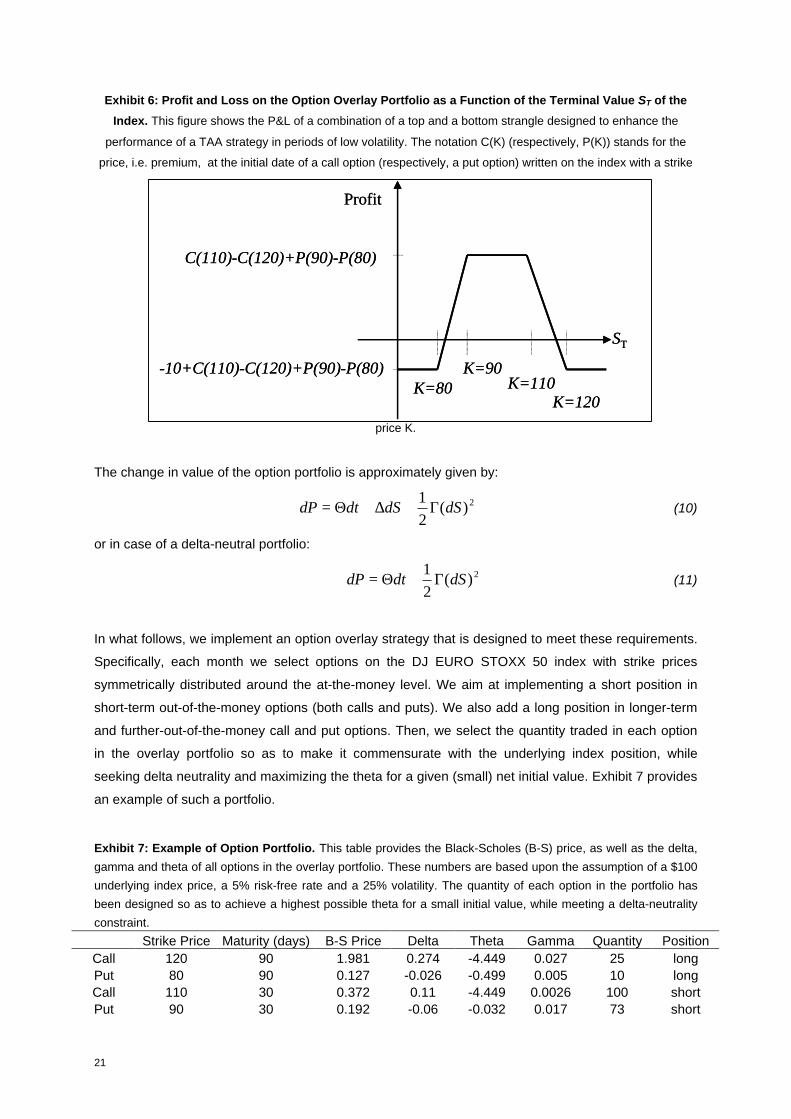
Exhibit 5: Profit and Loss on the Option Overlay Portfolio as a Function of the Terminal Value ST of the

Index. This figure shows the payoff as well as the P&L of a combination of a top and a bottom strangle designed

to enhance the performance of a TAA strategy in periods of low volatility. The notation C(K) (respectively, P(K))

stands for the price, i.e. premium, at the initial date of a call option (respectively, a put option) written on the index

with a strike price K.

ST<80 80<ST<90 90<ST<110 110<ST<120 120<ST

Payoff shortcall 110 0 0 0 -(ST-110) -(ST-110)Payoff shortput 90 -(90-ST) -(90-ST) 0 0 0Payoff TopStrangle ST-90 ST-90 0 110 -ST 110 -ST

P&L TopStrangle

ST-90+C(110)+P(90)

ST-90+C(110)+P(90) C(110)+P(90)

110-ST+C(110)+P(90)

110-ST+C(110)+P(90)

Payoff longcall 120 0 0 0 0 ST-120Payoff longput 80 80-ST 0 0 0 0PayoffBottomStrangle 80-ST 0 0 0 ST-120P&L BottomStrangle

80-ST-C(120)-P(80) -C(120)-P(80) -C(120)-P(80) -C(120)-P(80)

ST-120-C(120)-P(80)

PortfolioPayoff -10 ST-90 0 110 -ST -10

PortfolioP&L

-10+C(110)-C(120)+P(90)-

P(80)

ST-90+C(110)-C(120)+P(90)-

P(80)

C(110)-C(120)+P(90)-

P(80)

110-ST+C(110)-C(120)+P(90)-

P(80)

-10+C(110)-C(120)+P(90)-

P(80)

Exhibit 6 below shows the typical pay-off of this option portfolio as a function of the value of the

underlying asset at maturity.

21

Exhibit 6: Profit and Loss on the Option Overlay Portfolio as a Function of the Terminal Value ST of the

Index. This figure shows the P&L of a combination of a top and a bottom strangle designed to enhance the

performance of a TAA strategy in periods of low volatility. The notation C(K) (respectively, P(K)) stands for the

price, i.e. premium, at the initial date of a call option (respectively, a put option) written on the index with a strike

price K.

The change in value of the option portfolio is approximately given by:

2)(21

dSdSdtdP Γ+∆+Θ= (10)

or in case of a delta-neutral portfolio:

2)(21

dSdtdP Γ+Θ= (11)

In what follows, we implement an option overlay strategy that is designed to meet these requirements.

Specifically, each month we select options on the DJ EURO STOXX 50 index with strike prices

symmetrically distributed around the at-the-money level. We aim at implementing a short position in

short-term out-of-the-money options (both calls and puts). We also add a long position in longer-term

and further-out-of-the-money call and put options. Then, we select the quantity traded in each option

in the overlay portfolio so as to make it commensurate with the underlying index position, while

seeking delta neutrality and maximizing the theta for a given (small) net initial value. Exhibit 7 provides

an example of such a portfolio.

Exhibit 7: Example of Option Portfolio. This table provides the Black-Scholes (B-S) price, as well as the delta,

gamma and theta of all options in the overlay portfolio. These numbers are based upon the assumption of a $100

underlying index price, a 5% risk-free rate and a 25% volatility. The quantity of each option in the portfolio has

been designed so as to achieve a highest possible theta for a small initial value, while meeting a delta-neutrality

constraint.

Strike Price Maturity (days) B-S Price Delta Theta Gamma Quantity PositionCall 120 90 1.981 0.274 -4.449 0.027 25 longPut 80 90 0.127 -0.026 -0.499 0.005 10 longCall 110 30 0.372 0.11 -4.449 0.0026 100 shortPut 90 30 0.192 -0.06 -0.032 0.017 73 short

Profit

ST

K=80K=90

K=110K=120

-10+C(110)-C(120)+P(90)-P(80)

C(110)-C(120)+P(90)-P(80)

Profit

ST

K=80K=90

K=110K=120

-10+C(110)-C(120)+P(90)-P(80)

C(110)-C(120)+P(90)-P(80)

22

Portfolio -0.421 -0.03 326.349 -0.776

As can be seen from this example, we manage to obtain a portfolio with relatively low initial value

(dollar-neutral objective), with a net delta very close to zero (delta-neutral objective), for a relatively

low gamma and a high theta. The daily gain from holding this portfolio due to the time decay,

assuming the options are not exercised, is equal to 326.349/365= $0.894.

Exhibit 8 shows the value of the same portfolio a month later, assuming none of the options have been

exercised, and assuming that the underlying asset price, risk-free rate and volatility have remained at

a constant level.

Exhibit 8: Value of the Option Portfolio one Month Later. This table provides the Black-Scholes price, as well

as the delta, gamma and theta of all options in the overlay portfolio one month later. These numbers are based

upon the assumption of a $100 underlying index price, a 5% risk-free rate and a 25% volatility, and assuming that

none of the options have been exercised.

Strike Price Maturity (days) B&S Price Delta Theta Gamma Quantity PositionCall 120 60 0.201 0.049 -4.449 0.01 25 longPut 80 60 0.036 -0.01 -0.481 0.003 10 longCall 110 0 0 0 0 0 100 shortPut 90 0 0 0 0 0 73 short

Portfolio 5.385 1.125 -116.035 0.28

The gain from adding this option portfolio is 5.385 - (-0.421) = $5.806 over the one month period. This

addition generates a return enhancement for the TAA portfolio, without increasing the exposure of the

portfolio with respect to extreme risks thanks to the addition of the long position in the option portfolio.

Exhibit 9 shows the performance of this option overlay strategy…

Exhibit 4: Performance of TAA Strategies. This table contains information on the performance of the TAA

strategy with benchmark invested in cash when implemented on index futures. The mention NA (not applicable) is

displayed when the relevant performance measure does not apply to a particular portfolio.

Benchmark Libor TAA with Options TAA without OptionsCumulative Return 12.12% 27.51% 22.98%Annualized Return 3.82% 8.28% 7.07%Annualized Std Deviation 0.25% 5.58% 5.57%Sharpe 0.80 0.58Downside Risk (3.00%) 4.78% 4.46%Sortino (3.00%) 1.10 0.91% Negative Returns 13.89% 16.67%

To be completed

23

2. GENERATING ALPHAS THROUGH SECTOR ROTATION STRATEGIES

TAA strategies were traditionally concerned with allocating wealth between two asset classes, typically

shifting between stocks and bonds. More recently, more complex style timing strategies have been

successfully tested and implemented.

The Case for Tactical Style and Sector Allocation Strategies

These strategies are based on the recognition that Sharpe’s CAPM (1964) needs to be extended to

account for the presence of other pervasive risk factors, i.e., size and book-to-market factors (Fama

and French (1992)):

[ ]

[ ] [ ] {specific

,

style - systematic

,,,,,//,

market - systematic

,,,,,

titftsizesizeitftMBMBi

tftMMitfti

rRrR

rRrR

εββ

β

+−+−+

−=−

4444444 34444444 21

44 344 21

(12)

Such a decomposition of returns allows for a natural extended classification of active portfolio

strategies (see Exhibit 10). Market Timing or Tactical Asset Allocation Strategies aim at exploiting

evidence of predictability in market factor; Style Timing or Tactical Style Allocation (TSA) Strategies

aim at exploiting evidence of predictability in style factors; Stock Picking Strategies aim at exploiting

evidence of predictability in individual stock specific risk.

Exhibit 10: Classification of Active Portfolio Strategies

0X (systematic)

X (systematic)

TSA – long only

0X (systematic)

0TSA – market neutral

00X(discretionary or

systematic)

Mutual fund – market timing

XX (discretionary)

X (discretionary)

Mutual fund – stock picking

Stock pickingTactical Style Allocation

Tactical Asset Allocation

Form of active strategy

XX (discretionary)

0Hedge fund – stock picking

SpecificSystematic - styleSystematic - market

0X (systematic)

X (systematic)

TSA – long only

0X (systematic)

0TSA – market neutral

00X(discretionary or

systematic)

Mutual fund – market timing

XX (discretionary)

X (discretionary)

Mutual fund – stock picking

Stock pickingTactical Style Allocation

Tactical Asset Allocation

Form of active strategy

XX (discretionary)

0Hedge fund – stock picking

SpecificSystematic - styleSystematic - market

24

It is perhaps surprising that, on the one hand, most long/short equity managers still favor stock picking

as a way to generate abnormal return, while, on the other hand, thirty years of academic studies have

shown that there is little evidence of predictability in the specific component of stock returns in the

absence of private information. It should be noted that TSA is not a new concept. Most mutual fund

managers actually make discretionary, and sometimes unintended, bets on styles as much as they

make bets on stocks. In other words, they perform TAA, TSA and stock picking at the same time in a

somewhat confusing “mélange des genres”. As in many other contexts, we have evidence that

specialization pays. In particular, Daniel, Grinblatt, Titman and Wermers (1997] find evidence that

mutual funds showed some stock selection ability, but no discernable ability to time the different stock

characteristics in terms of book-to-market or size.

More recently, several authors have emphasized the benefits of focusing on style timing exclusively. In

particular, Fan (1995), Sorensen and Lazzara (1995), Kao and Shumaker (1999), Avramov (2000) or

Bauer and Molenaar (2002) report strong evidence of predictability in equity style returns and

underline the performance of strategies that involve dynamic trading in various equity styles. Related

papers also include Gerber (1994), Case and Cusimano (1995), Fisher, Toms and Blount (1995), Mott

and Condon (1995), Levis and Liodakis (1999), Oertmann (1999), Reiganum (1999), Amenc and

Martellini (2001), Cooper et al. (2001), Ahmed, Lockwood and Nanda (2002), Amenc, El Bied and

Martellini (2003), or Amenc et al. (2003).

In a similar spirit, Cavaglia and Moroz (2002) provide evidence that local industry returns are

predictable. They present the performance of simulated strategies and demonstrate that active sector

rotation across countries provides an additional source of alpha beyond simplistic country rotation

strategies. They present a forecasting approach to predicting the relative performance of industries in

each of 22 developed country equity markets and demonstrate that a blend of style signals provides

an effective way to predict the return performance of these assets. The out-of-sample portfolio

performance of investment strategies based on these forecasts for the 1991-2001 period would have

provided annual gross returns in excess of the world benchmark return of 400 bps a year with one-way

turnover of 50 percent.

In a related paper, Johnson and Sakoulis (2003) show how financial and economic variables can be

employed in a time varying dynamic sector allocation model for U.S. equities. They find that using the

Kalman filter to estimate time varying sensitivities to predetermined risk factors results in significantly

improved sector return predictability over static or rolling parameter specifications. A simple trading

strategy developed here using Kalman filter predicted returns as input provides for potentially robust

long run profit opportunities.

Sorensen and Burke (1986) and Beller, Kling, and Levinson (1998) also found that U.S. industry

returns can be predicted by using either past return performance or macroeconomic fundamentals;

they cautioned, however, that the extent of asset return predictability may not offset transaction costs

25

sufficiently to maintain the paper profits when their models are implemented. Capaul (1999) found

conflicting evidence about the effectiveness of using traditional style factors for global industries. For

instance, he found that low-P/B (price-to-book) industries underperformed high-P/B industries in the

1991-98 period; similarly, buying “large” global industries appeared to be more attractive than buying

“small” global industries.

Implementing Sector Rotation Strategies using Eurex Sector Index Futures

While active sector rotation is a popular strategy among investors, it is operationally intensive and

expensive when implemented with individual stocks. In what follows, we argue that futures on sector

indexes are a natural cost-efficient way for active sector rotation.

In this section, we design a long/short strategy that generates abnormal return from timing between

various sectors of a European index while maintaining a zero exposure with respect to the global

index.

In an effort to calibrate models on asset classes for which liquid investible products are available, we

have chosen to focus on the following two sector indices, DJ EURO STOXX Banks and DJ EURO

STOXX Telecom. Investible products (futures and options) on these indices were introduced by Eurex

in March 2001.

Given that we are searching for evidence of predictability in equity style returns with the goal of

implementing a sector rotation strategy, we focus on the best possible trade-off between quality of fit

and robustness. We show how to implement a systematic sector strategy on the basis of a

sophisticated econometric approach similar to the one used in the context of the DJ EURO STOXX 50

TAA strategy.xiii

The results we obtain are summarized in Exhibit 11. The average hit ratio over the period is equal to

64%, which is significantly greater than 50% (null hypothesis of no predictability) at the 5% level.

Interestingly, if we exclude cases when the average forecast probability is less than one standard

deviation away from 50% (i.e., numbers in italic and boldfaced in column 6), the hit ratio reaches a

spectacular 0.875 value (over 16 months).

26

Exhibit 11: Econometric Forecasts for a Sector Rotation Strategy. In column 2 information can be found on

the number of models in the council at each date after application of various filters. Column 3 tells us about the

level of t-stat across models and variables. Column 4 is the average forecast probability; it provides information

about the predicted sign (prediction that the DJ EURO STOXX Bank index outperforms the DJ EURO STOXX

Telecom Index when the value is higher than 50%). Column 5 contains a measure of dispersion of different

models’ forecasts (standard deviation of forecast probabilities). Column 6 provides hit ratios (equal to 1 if the

correct sign is forecast, equal to 0 otherwise). Numbers in italic and boldfaced relate to cases when the average

forecast probability is less than a standard deviation away from 50%.

Date No of Models Average T-Stat Prob(y>0) Sigma Hit Ratio

Aug-00 2 2.34 68.98% 21.99% 1Sep-00 2 2.41 48.34% 5.05% 0Oct-00 3 2.45 62.38% 2.71% 1Nov-00 3 2.53 27.65% 5.29% 1Dec-00 2 2.54 89.21% 2.48% 1Jan-01 3 2.62 68.26% 11.12% 1Feb-01 3 2.64 92.44% 4.34% 1Mar-01 1 2.48 92.97% 0.00% 1Apr-01 3 2.43 57.75% 28.29% 1May-01 8 2.48 90.45% 4.61% 1Jun-01 8 2.58 98.61% 1.95% 1Jul-01 8 2.58 88.58% 4.86% 1Aug-01 10 2.60 65.61% 15.31% 0Sep-01 10 2.63 69.11% 12.46% 1Oct-01 10 2.65 25.63% 17.43% 1Nov-01 11 2.73 60.64% 18.80% 0Dec-01 8 2.72 80.37% 7.28% 0Jan-02 6 2.75 43.52% 18.28% 0Feb-02 11 2.66 38.23% 20.80% 0Mar-02 9 2.65 29.09% 16.41% 1Apr-02 3 2.71 53.32% 3.89% 1May-02 4 2.79 60.15% 4.17% 1Jun-02 7 2.86 56.51% 6.16% 1Jul-02 10 2.73 56.24% 12.05% 0Aug-02 10 2.68 56.98% 16.82% 0Sep-02 9 2.82 56.15% 12.35% 0Oct-02 8 2.80 67.28% 22.72% 0Nov-02 6 2.73 61.86% 16.95% 1Dec-02 9 2.82 70.77% 23.78% 0Jan-03 8 2.80 59.39% 22.07% 1Feb-03 8 2.71 58.40% 23.10% 0Mar-03 10 2.64 45.55% 26.72% 0Apr-03 12 2.51 45.36% 29.59% 1May-03 13 2.59 50.90% 34.03% 1Jun-03 9 2.70 63.97% 23.99% 1Jul-03 8 2.68 58.49% 19.45% 1

27

Our portfolio process is similar to the one introduced in a TAA context. More specifically, we use the

following rules to define a market-neutral sector rotation strategy:2

• If the average forecast probability is more than one standard deviation away from 50%, the

allocation to the DJ EURO STOXX Bank index is equal to mp-50% and the allocation to the

DJ EURO STOXX Telecom index is equal to 50%-mp.

• If the average forecast probability is less than one standard deviation away from 50%, the

allocation to the DJ EURO STOXX Bank index equals (mp-50%)/2 and the allocation to the DJ

EURO STOXX Telecom index equals (50%-mp)/2.

We have also tested a more aggressive version of this portfolio process, where the allocation to the DJ

EURO STOXX Bank index is equal to 2(mp-50%) and (mp-50%), in the higher and lower confidence

cases, respectively. In exhibit 12 an overview of the results can be found.

Exhibit 12: Performance of a Sector Rotation Strategy. This table contains information on the performance of

a sector rotation strategy (bank sector versus telecom sector) for 2 levels of aggressiveness, as described in the

body of the text. The mention NA (not applicable) is displayed when the relevant performance measure does not

apply to a particular portfolio.

Benchmark = One-Month Libor Less Aggressive More AggressiveCumulative Return 12.12% 41.46% 77.04%Annualized Return 3.82% 11.74% 19.66%Annualized Std Deviation 0.25% 5.12% 10.11%Sharpe NA 1.547 1.567% Negative Returns NA 11.11% 19.44%Worst Monthly Drawdown NA -1.09% -2.44%

Mixing TAA and Sector Rotation Benefits

In this section, we also consider the benefits of a double-alpha strategy involving both TAA and sector

rotation decisions. We focus on the case of the benchmark invested 100% in cash for the TAA

strategy, and a less aggressive portfolio process in both cases. The results are displayed in exhibit 13.

Exhibit 13: Performance of a Strategy Mixing Sector Rotation and TAA. This table contains information on

the performance of a strategy mixing sector rotation (bank sector versus telecom sector) and TAA in the less

aggressive version, as described in the body of the text. The mention NA (not applicable) is displayed when the

relevant performance measure does not apply to a particular portfolio.

Benchmark = One-Month LiborDJ EURO STOXX Sector

Rotation

Less Aggressive DJEURO STOXX + One-

Month Libor Composite PortfolioCumulative Return 12.12% 41.46% 27.52% 34.65%Annualised Return 3.82% 11.74% 8.28% 10.01%Annualised Std Deviation 0.25% 5.12% 5.55% 3.32%Sharpe NA 1.547 0.804 1.866

2 Market neutral can imply dollar-neutrality or beta-neutrality. Here we consider dollar-neutrality for simplicity of exposure.

28

% Negative Returns NA 11.11% 13.89% 11.11%Worst Monthly Drawdown NA -1.09% -3.39% -1.45%

As can be seen from Exhibit 13, mixing asset and sector allocation decisions allows one to

significantly lower the portfolio volatility while maintaining the level of average returns. This is due to

the benefits of bet diversification: active asset and sector allocation bets are wrong in about one-third

of the cases, but they are not necessarily wrong on the same dates.

CONCLUSION

In this paper, we explain how active portfolio managers, who attempt to generate abnormal profits

through bets on well-identified risks for which they feel they have reliable views, can benefit from using

suitably packaged derivatives satellite portfolios as portable alpha and beta vehicles.

These portfolios, based on active asset allocation decisions, can be used either as standalone

absolute return alpha providers, or as overlay portfolios customized to help them modify the exposure

of their portfolios with respect to a variety of sources of risks on which they have no desire to bet. In

particular, we provide an example of a short volatility strategy that allows a manager to enhance the

performance of a base investment strategy.

The benefits of active asset allocation decisions that we present in this experiment are not based on

the use of any specific econometric model with unusually superior predictive power. The approach

followed in this paper is actually based on a process that consists of selecting at each date a “council”

of models to make predictions, as opposed to using a single model. We actually believe that the

benefits of active asset allocation decisions originate more from the combination of a robust

econometric process and an efficient trading of low cost investible products such as Eurex index

futures and options, rather than the use of any given mysterious model with extraordinary

performance. This strongly suggests that most long-short managers could use a similar methodology

to enhance the performance of their portfolios.

REFERENCES

Ahmed, P., L. Lockwood, and S. Nanda, 2002, Multistyle rotation strategies, Journal of Portfolio

Management, Spring, 17-29.

Aiolfi, M., and C. Favero, 2002, Model Uncertainty, Thick Modeling and the Predictability of Stock

Returns, working paper, Bocconi University.

Amenc, N., S. El Bied and L. Martellini, 2003, Evidence of predictability in hedge fund returns and

multi-style multi-class style allocation decisions, Financial Analysts Journal, 5, 59, 32-46.

29

Amenc, N., P. Malaise, L. Martellini, and D. Sfeir, 2003, Tactical style allocation: a new form of market

neutral strategy, Journal of Alternative Investments, 6, 1, 8-22.

Amenc, N., and L. Martellini, 2001, It’s time for asset allocation, Journal of Financial Transformation, 3,

77-88.

Arnott, R., and T. Miller, 1996, Using options in a TAA process, Investment Management Reflection,

Internal Document, First Quadrant.

Avramov, D., 2002, Stock return predictability and model uncertainty, Journal of Financial Economics,

64, 3, 423-458.

Barberis, N., 2000, Investing for the long run when returns are predictable, Journal of Finance, 55,

225-264.

Bauer, R., and R. Molenaar, 2002, Is the value premium predictable in real time?, working paper,

Maastricht University.

Beller, K., J. Kling, and M. Levinson, 1998, Are industry stock returns predictable?, Financial Analysts

Journal, 54, 5, 42-57.

Bossaerts, P., and P., Hillion, 1999, Implementing statistical criteria to select return forecasting

models: what do we learn?, The Review of Financial Studies, 12, 2, 405-428.

Brandt, M., 1999, Estimating portfolio and consumption choice: a conditional Euler equations

approach, Journal of Finance, 54, 1609-1645.

Brennan, M., E. Schwartz and R. Lagnado, 1997, Strategic asset allocation, Journal of Economic

Dynamics and Control, 21, 1377-1403.

Campbell, J., 2000, "Asset pricing at the Millenium", Journal of Finance, 55, 1515-1567.

Campbell, J., Y. Chan, and L. Viceira, 2000, A multivariate model of strategic asset allocation, Working

Paper, Harvard University.

Campbell, J., and R. Shiller, 1988, Stock prices, earnings, and expected dividends, Journal of

Finance, 43, 661-676.

Capaul, C., 1999, Asset-pricing anomalies in global industry indexes, Financial Analysts Journal, 55,

4, 17-37.

30

Case, D., and S., Cusimano, 1995, Historical tendencies of equity style returns and the prospects for

tactical style allocation, chapter 12 from Equity Style Management, Irwin Publishing.

Cavaglia, S., and V. Moroz, 2002, Cross-industry, cross-country allocation, Financial Analysts Journal,

58, 6, 78-97.

Cochrane, J., 2000, Asset Pricing, Princeton University Press.

Cooper, M., Gulen, H., and M. Vassalou, 2001, Investing in size and book-to-market portfolios using

information about the macroeconomy: some new trading rules, working paper, Graduate School of

Business, Columbia University.

Daniel, K., Grinblatt, M., Titman S., and Wermers, S., 1997, Measuring mutual fund performance with

characteristic based benchmarks, Journal of Finance, 52, 3, 1035-1058.

Doppelhofer, G., Miller, R., Sala-i-Martin, 2000, Determinants of long-term growth:a Bayesian

averaging of classical estimates(BACE) approach ’, NBER working paper 7750.

Fama, E., 1981, Stock returns, real activity, inflation, and money, American Economic Review, 545-

565.

Fama, E., and W. Schwert, 1977, Asset returns and inflation, Journal of Financial Economics, 115-46.

Fama, E., and K. French, 1989, Business conditions and expected returns on stocks and bonds,

Journal of Financial Economics, 25, 23-49.

Fama, E., and K. French, 1992, The cross-section of expected stock returns, Journal of Finance, 442-

465.

Fama, E., and K. French, 1998, Value versus growth: the international evidence, Journal of Finance,

53, 6, 1975-2000.

Fan, S., 1995, Equity style timing and allocation, chapter 14 from Equity Style Management, Irwin

Publishing.

Ferson, W., and C. Harvey, 1991, Sources of predictability in portfolio returns, Financial Analysts

Journal, May/June, 49-56.

31

Ferson, W., and C. Harvey, 1993, The risk and predictability of international equity returns, Review of

Financial Studies, 6, 527- 566.

Ferson, W., and C. Harvey, 1995, Predictability and time-varying risk in world equity markets,

Research in Finance, 13, 25-88.

Fisher, K., J., Toms, and K., Blount, 1995, Driving factors behind style-based investing, chapter 22

from Equity Style Management, Irwin Publishing.

Gerber, G.,. 1994, Equity style allocations: timing between growth and value, in Global Asset

Allocation: Techniques for Optimizing Portfolio Management. New York: John Wiley & Sons.

Ghysels, E., 1998, On stable factor structure in asset pricing: Do time-varying betas help or hurt?

Journal of Finance, 53, 549-573.

Glosten, L., R. Jagannathan, and D. Runkle, 1993, On the relation between the expected value and

the volatility of the nominal excess return on stocks, Journal of Finance, 48, 1779-1801.

Hamilton, J., 1994, Time series analysis, Princeton University Press.

Harasty, H., and J. Roulet, 2000, Modelling stock market returns - an error correction model, Journal

of Portfolio Management, Winter, 33-46.

Harvey, C., 1989, Time-varying conditional covariances in tests of asset pricing models, Journal of

Financial Economics, 24, 289-317.

Harvey, C., 1995, Predictable risk and returns in emerging markets, Review of Financial Studies, 773-

816.

Haugen, R., and J., Lakonishok, 1988, The incredible January effect--The stock market's unsolved

mystery, Homewood, IL: Dow Jones-Irwin.

Jarque, C. and A. Bera, 1980, Efficient tests for normality, homoskedasticity, and serial independence

of regression residuals, Economics Letters, 6, 255–259.

Johnson L., and G. Sakoulis, 2003, Maximizing equity market sector predictability in a dynamic time

varying parameter model, working paper, J.P Morgan Fleming Asset Management.

Kandel, S., and R. Stambaugh, 1996, On the predictability of stock returns: an asset allocation

perspective, Journal of Finance, 51, 385-424.

32

Keim, D., and R. Stambaugh, 1986, Predicting returns in the stock and bond markets, Journal of

Financial Economics, 17, 357-390.

Lee, W., 2000, Advanced theory and methodology of tactical asset allocation, Fabozzi and Associates

Publications.

Levis, M., and M., Liodakis, 1999, The profitability of style rotation strategies in the United Kingdom,

Journal of Portfolio Management, 26 (Fall), 73-86.

Leung, M., Daouk, H., and A.-S. Chen, 2000, Forecasting stock indices: a comparison of classification

and level estimation models, International Journal of Forecasting, 16, 173-190.

Lynch, A., 2000, Portfolio choice and equity characteristics: characterizing the hedging demands

induced by return predictability, working paper, NYU.

Lynch, A., and P. Balduzzi, 1999, Predictability and transaction costs: the impact on rebalancing rules

and behavior, forthcoming, Journal of Finance.

Merton, R. C., 1969, Lifetime portfolio selection under uncertainty: the continuous-time case, Review

of Economics and Statistics, 51, 247-257.

Merton, R. C., 1971, Optimal consumption and portfolio rules in a continuous-time model, Journal of

Economic Theory, 3, 373-413.

Merton, R. C., 1973, An intertemporal capital asset pricing model, Econometrica, 41, 867-888.

Mott, C., and K., Condon, 1995, Exploring the cycles of small-cap style performance, chapter 9 from

Equity Style Management, Irwin Publishing.

Oertmann, P., 1999, Why do value stocks earn higher returns than growth stocks, and vice-versa?,

working paper, Investment Consulting Group Inc. and University of St. Gallen.

Pesaran, M., and A. Timmerman, 1995, Predictability of stock returns: robustness and economic

significance, Journal of Finance, 50, 1201-1228.

Philip, T., G. Rogers, and R. Capaldi, 1996, Tactical asset allocation: 1977-1994, Journal of Portfolio

Management, 57-64.

Reignaum, M., 1999, The significance of market capitalization in portfolio management over time,

Journal of Portfolio Management, 25 (Summer), 39-50.

33

Samuelson, P., 1969. Lifetime portfolio selection by dynamic stochastic programming, Review of

Economics and Statistics, 51, 239-246.

Sharpe, W., 1964, Capital Asset Prices: a Theory of Market Equilibrium under Conditions of Risk,

Journal of Finance, 19, 425-442.

Sorensen, E., and T. Burke, 1986, Portfolio returns from active industry group rotation, Financial

Analysts Journal, 46, 5, 43-50.

Sorensen, E., and C. Lazzara, 1995, Equity style management: the case of growth and value, chapter

4 from Equity Style Management, Irwin Publishing.

i On the other hand, some long-short managers use quantitative techniques to implement a systematicrisk management process allowing them to actively manage their exposure to a variety of risk factors.ii Ideally, one would like to account for both the presence of no- linear dependencies and dynamiccoefficients. There is however few examples of tractable non-linear dynamic models.iii The Goldman Sachs Commodity Index is a world production-weighted commodity index comprisedof 25 liquid, exchange-traded futures contracts.iv The US $ major currency index is a daily trade-weighted currency index which measures nominalexchange rate strength of the US dollar relative to a basket consisting of Canada, Japan, Euro,Denmark, Norway, Sweden, Switzerland, UK, Mexico, Australia, New Zealand, China, Hong Kong,Korea, Singapore and Taiwan.v One may also include economic variables. One problem there is the risk of posterior adjustment,which refers to the fact that the estimate of an economic variable (e.g., inflation) for a previous datecan be adjusted several months after a first estimate is first released. As a result, economic series indatabases may contain cleaner data than what is actually available in real-time.vi In principle, we could have used a longer time-period, but this would have severely limited thenumber of variables that could be included in the analysis. Given that our emphasis is on economicimpact of predictability, we have chosen to focus on a process that can be similar to the one thatwould be used in actual investment practice.vii We would have rather used the Dividend Yield on the DJ EuroStoxx index, but that data was notavailable to us.viii Hit ratios are the percentage of times the predicted sign equals the actual sign of the style return.We test whether hit ratios are significantly greater than ½ (benchmark case of no model): in the caseof 24 observations, a hit ratio of at least 63% (respectively, 67%) is significantly greater than ½ at the10% (respectively, 5%) level. We also compute the associated t-statistics to check whether thevariable had a statistically significant explanatory power.ix It is well known (e.g., Stambaugh (1999)) that asymptotic distribution theory on which statisticalinference is based provides a poor approximation to the actual finite-sample distribution of test-statistics when the predictor is persistent. To avoid spurious regression problems, it is therefore usefulto check whether the independent and dependent variables are stationary, using a standard unit roottest, the Dickey-Fuller (1979) test (see also and Phillips and Perron (1988)).x We have also checked that multi-colinearity was not an issue, as the maximum correlation betweentwo variables does not exceed 60% in the sample.xi By August 2000, we mean a forecast performed on July 7th, for the period ranging from July 7th toAugust 7th.xii A similar strategy is presented in Arnott and Miller (1996), with the difference that no optimisation isperformed over the composition of the portfolio.xiii One difference is that we had to increase the number of variables used in the process from August2000 to March 2002 as there was no model before April 2002 that could meet the criteria when welimited ourselves to the 10 variables used in a TAA context.