porosity characterization utilizing petrographic image
TRANSCRIPT

i
POROSITY CHARACTERIZATION UTILIZING PETROGRAPHIC
IMAGE ANALYSIS: IMPLICATIONS FOR IDENTIFYING AND
RANKING RESERVOIR FLOW UNITS, HAPPY SPRABERRY
FIELD, GARZA COUNTY, TEXAS
A Thesis
by
JOHN MORGAN LAYMAN II
Submitted to the Office of Graduate Studies ofTexas A&M University
in partial fulfillment of the requirements of the degree of
MASTER OF SCIENCE
May 2002
Major Subject: Geology

ii
POROSITY CHARACTERIZATION UTILIZING PETROGRAPHIC
IMAGE ANALYSIS: IMPLICATIONS FOR IDENTIFYING AND
RANKING RESERVOIR FLOW UNITS, HAPPY SPRABERRY
FIELD, GARZA COUNTY, TEXAS
A Thesis
by
JOHN MORGAN LAYMAN II
Submitted to Texas A&M Universityin partial fulfillment of the requirements
for the degree of
MASTER OF SCIENCE
Approved as to style and content by:
__________________________ _________________________ Wayne M. Ahr Steven L. Dorobek (Chair of Committee) (Member)
______________________________ _____________________________ Thomas A. Blasingame Andrew Hajash, Jr. (Member) (Head of Department)
May 2002
Major Subject: Geology

iii
ABSTRACT
Porosity Characterization Utilizing Petrographic Image Analysis: Implications for
Identifying and Ranking Reservoir Flow Units, Happy Spraberry Field, Garza County,
Texas. (May 2002)
John Morgan Layman II, B.S., James Madison University
Chair of Advisory Committee: Dr. Wayne M. Ahr
The Spraberry Formation is traditionally thought of as deep-water turbidites
in the central Midland Basin. At Happy Spraberry field, Garza County, Texas, however,
production is from a carbonate interval about 100 feet thick that has been correlated on
seismic sections with the Leonardian aged, Lower Clear Fork Formation. The “Happy
field” carbonates were deposited on the Eastern Shelf of the Midland Basin and consist
of oolitic skeletal grainstones and packstones, rudstones and floatstones, in situ
Tubiphytes bindstones, and laminated to rippled, very-fine grained siltstones and
sandstones. The highest reservoir “quality” facies are in the oolitic grainstones and
packstones where grain-moldic and solution-enhanced intergranular porosity dominate.
Other pore types present include incomplete grain moldic, vuggy, and solution-enhanced
intramatrix.
The purpose of this study was to relate pore geometry measured by digital
petrographic image analysis to petrophysical characteristics, and finally, to reservoir
quality. Image analysis was utilized to obtain size, shape, frequency, and total

iv
abundance of pore categories. Pore geometry and percent porosity were obtained by
capturing digital images from thin sections viewed under a petrographic microscope.
The images were transferred to computer storage for processing with a commercial
image analysis program trademarked as Image Pro Plus (Version 4.0).
A classification scheme was derived from the image processing enabling “pore
facies” to be established. Pore facies were then compared to measured porosity and
permeability from core analyses to determine relative “quality” of reservoir zones with
different pore facies. Pore facies are defined on pore types, sizes, shapes, and
abundances that occur in reproducible associations or patterns. These patterns were
compared with porosity and permeability values from core analyses. Four pore facies
were identified in the Happy field carbonates; they were examined for evidence of
diagenetic change, depositional signatures, and fractures. Once the genetic categories
were established for the four pore facies, the pore groups could be reexamined in
stratigraphic context and placed in the stratigraphic section across Happy field. Finally,
the combined porosity and permeability values characteristic of each pore facies were
used to identify and rank good, intermediate, and poor flow units at field scale.

v
ACKNOWLEDGEMENTS
I would like to thank the AAPG Foundation, Mr. Michel T. Halbouty, and Texas
A&M University for providing funding for this project, without which, the science and
presentation of this study would not have been a success.
I wish to thank my advisor, Dr. Wayne Ahr, for access to all of the pertinent data
for this project. He provided encouragement, enthusiasm, and was my guide when I
entered uncharted territory during this study. Dr. Steve Dorobek provided insight into
carbonate sedimentology and image analysis techniques which proved very helpful. Dr.
Tom Blasingame provided an alternate vista from the petroleum-engineering standpoint
and was helpful in Clear Fork Formation evaluation.
I would also like to thank my fellow graduate students who made all of this
bearable, and, at times, enjoyable. Special thanks to Bo and Elizabeth Slone, Jared
Haight, John Leone, and everyone else on the ground floor of Halbouty. Your support,
discussions, advice, and friendship kept me sane.
Finally, I want to express thanks to Mom and Dad, Regina and Rhonda, and the
rest of my family for all of their support throughout this endeavor. You have always
encouraged me with love, patience, and understanding and I owe much of my success to
you. Thank you.

vi
TABLE OF CONTENTS
Page
ABSTRACT ..................................................................................................................... iii
ACKNOWLEDGEMENTS ...............................................................................................v
TABLE OF CONTENTS ................................................................................................. vi
LIST OF FIGURES........................................................................................................ viii
LIST OF TABLES ........................................................................................................... xi
INTRODUCTION..............................................................................................................1
Purpose of Study ...................................................................................................1
Location of Study Area ..........................................................................................2
REGIONAL GEOLOGIC SETTING ................................................................................7
Structure .................................................................................................................7
Stratigraphy ............................................................................................................8
PREVIOUS WORK .........................................................................................................10
Happy Spraberry Field .........................................................................................10
Petrographic Image Analysis (PIA) .....................................................................11
Nature of This Study ............................................................................................12
METHODS.......................................................................................................................14
Lithological Study ................................................................................................14
Borehole Logs ......................................................................................................15
Thin-Section Petrography ....................................................................................15
Petrographic Image Analysis (PIA) .....................................................................16

vii
Page
RESULTS.........................................................................................................................23
Lithofacies............................................................................................................23
Depositional Environment....................................................................................29
Log Analysis ........................................................................................................30
Core Analysis .......................................................................................................31
Thin-Section Petrography ....................................................................................33
Genetic Classification of Carbonate Pores...........................................................34
Pore Types............................................................................................................36
Petrographic Image Analysis (PIA) .....................................................................41
Mercury Injection Capillary Pressure (MICP) .....................................................52
DISCUSSION ..................................................................................................................56
Total Porosity ......................................................................................................56
Pore Data and Pore Facies....................................................................................66
Petrographic Image Analysis Predicting Capillary Pressure Behavior ................71
CONCLUSIONS..............................................................................................................79
REFERENCES CITED ....................................................................................................81
APPENDIX A ..................................................................................................................85
APPENDIX B ................................................................................................................100
VITA ..............................................................................................................................103

viii
LIST OF FIGURES
Figure Page
1. Regional paleo-map of the Permian Basin, west Texas-southeasternNew Mexico ...........................................................................................................4
2. Happy Spraberry field base map showing location of wells and theJohn F. Lott lease ...................................................................................................5
3. Generalized stratigraphic cross-section of the Midland Basin-EasternShelf transition .......................................................................................................6
4. Shelf to basin stratigraphic correlation...................................................................9
5. Screen capture of Image Pro Plus image analysis software ...............................17
6. Calibration slide image.........................................................................................18
7. Schematic of thin-section sampling .....................................................................19
8. Measurement window ..........................................................................................21
9. Auto classification window..................................................................................22
10. Core photos of oolitic and skeletal grainstone .....................................................24
11. Core photo of floatstone.......................................................................................25
12. Core photo of rudstone.........................................................................................26
13. Core photo of Tubiphytes bindstone.....................................................................27
14. Core photo of siltstone .........................................................................................28
15. Type log for Happy field, Lott 19 #4 ...................................................................32
16. Porosity classification system ..............................................................................35
17. Photomicrographs of moldic and incomplete moldic pores.................................36
18. Photomicrographs of solution enhanced intergranular pores ...............................37

ix
Figure Page
19. Photomicrograph of solution enhanced intramatrix pores ...................................38
20. Photomicrograph of vuggy pores .........................................................................39
21. Photomicrograph of intraparticle pores................................................................40
22. Photomicrograph of primary intergranular pores.................................................41
23. Photomicrographs of Lott 19 #4 well, 4960.6’ ....................................................43
24. Frequency histogram of Lott 19 #4 well, 4960.6’................................................44
25. Lott 19 #4 well, 4923.8’ photomicrographs and histogram .................................46
26. Lott 19 #7 well, 4978.9’ photomicrographs and histogram .................................47
27. Lott 19 #7 well, 4981.2’ photomicrographs and histogram .................................49
28. Lott 19 #7 well, 4950.8’ photomicrographs and histogram .................................50
29. Lott 19 #4 well, 4971.4’ photomicrographs and histogram .................................51
30. Summary of PIA data ...........................................................................................54
31. Pore throat size distribution..................................................................................55
32. Core porosity vs. core permeability .....................................................................58
33. Core porosity vs. core permeability with lithofacies............................................59
34. Core porosity vs. petrographic porosity ...............................................................60
35. Petrographic porosity by standard methods vs. image analysis porosity .............61
36. Core porosity vs. image analysis porosity............................................................63
37. Image analysis porosity vs. wireline log porosity ................................................64
38. Lott 19 #4 well porosity comparison....................................................................65
39. Legend for pore facies model stratigraphic cross-section ...................................68

x
Figure Page
40. Stratigraphic cross section incorporating pore facies model................................70
41. Median throat diameter vs. core permeability......................................................72
42. Image analysis porosity vs. median throat diameter ............................................73
43. Image analysis porosity vs. core permeability .....................................................74
44. Median pore throat vs. median pore size..............................................................77
45. Photomicrograph of non-touching vugs...............................................................78

xi
LIST OF TABLESTable Page
1. Shape interpretation table........................................................................................20
2. Excel spreadsheet of pore data ................................................................................42
3. Summary of data from ten additional thin sections..................................................75

1
INTRODUCTION
Carbonate reservoirs are commonly heterogeneous; consequently, they may
require special methods and techniques for description and evaluation. Reservoir
characterization, in its strictest sense, is the study of the reservoir rocks, their
petrophysical properties, the fluids they contain – or the manner in which they influence
the movement of fluids in the subsurface. This study focuses on the description of rocks
and the pore network of a carbonate reservoir interval located at Happy Spraberry field,
Garza County, Texas. Porosity and permeability relationships, wireline log signature,
and a limited number of capillary pressure measurements have been examined to
determine how the various factors influence reservoir quality. This study utilized a color
video camera attached to a petrographic scope for acquiring pore images in thin section,
and Image Pro Plus image analysis software to acquire and process pore data gathered
in the petrographic image analysis study.
Purpose of Study
The purpose of this study is to assess the reliability and value of digital image
analysis of carbonate pores as a predictor of reservoir quality and performance. In order
to accomplish this task, carbonate pores were examined in thin section to establish
categories based on size, shape, and abundance. The categories were then tested to
This thesis follows the style and format of the American Association of Petroleum Geologists Bulletin.

2
determine the extent to which they correspond with other indicators of reservoir quality
such as measured porosity, permeability, and capillary pressures. Visible porosity in
each of the selected thin sections was compared to measured porosity from core
analyses, porosity derived from wireline logs, and porosity from “hand counts” on thin
sections (without image analysis). Pore measurements made with image analysis
techniques were grouped on geometry and abundance and checked for geologic origin
(genetic pore classification). Pore facies were developed to identify patterns in the
porosity and petrophysical characteristics in the Happy field reservoir.
A geological model was constructed based on the origin and spatial distribution
of the reservoir pore types. Studies by Hammel (1996) and Roy (1998) aided in the
development of a technique for determining and comparing the best, intermediate, and
poorest reservoir zones, or flow units. The results of this study suggest that automated
image analysis can provide rapid and reliable measurements of pore geometry and
abundance that enable the construction of reservoir pore facies. The pore facies, in turn,
can be mapped to identify reservoir zones and reservoir quality. The entire process can
be accomplished in a fraction of the time required to examine thin sections by the
conventional “by hand” method.
Location of Study Area
Happy Spraberry field is located in Section 19, Block 2, T. & N.O.R.R. Co.
Survey, Garza County, Texas on the western edge of the Eastern Shelf (Figure 1). The
field is in the John F. Lott lease and includes 15 wells (Figure 2), that produce from a

3
carbonate interval about a 100 feet thick and presently at an average depth of about
5,000 feet below present sea-level. The reservoir consists of in situ, shallow marine
oolitic/skeletal packstones and grainstones, floatstones, rudstones, Tubiphytes
bindstones, siltstones, and very-fine grained sandstones. Although called Happy
Spraberry field, the carbonate interval is not part of the Spraberry Formation. The
Spraberry trend of siliciclastic turbidite deposits is located 150 miles southwest of
Happy field in the central Midland Basin. The carbonate interval at Happy field is Early
Permian (lower Leonardian) in age and is interpreted to be part of the Lower Clear Fork
Formation (Tranckino, pers. comm.). The Lower Clear Fork Formation is in fact,
approximate time equivalent to the basinal Dean Formation (Figure 3).
4
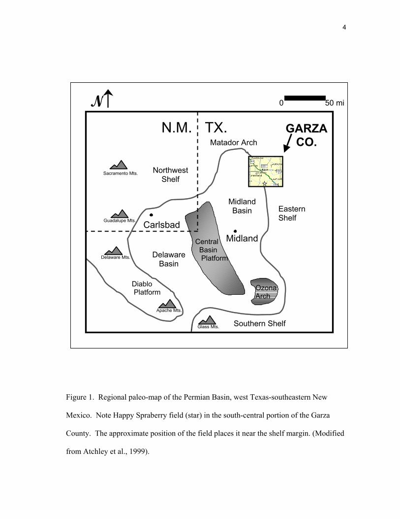
Figure 1. Regional paleo-map of the Permian Basin, west Texas-southeastern New
Mexico. Note Happy Spraberry field (star) in the south-central portion of the Garza
County. The approximate position of the field places it near the shelf margin. (Modified
from Atchley et al., 1999).
MidlandBasin
DelawareBasin
NorthwestShelf
EasternShelf
Central Basin Platform
Ozona Arch
Matador Arch
Diablo Platform
Southern Shelf
Midland
Delaware Mts.
Guadalupe Mts.
Apache Mts.
Sacramento Mts.
Glass Mts.
Carlsbad
N.M. TX. GARZACO.
0 50 miN

5
Figure 2. Happy Spraberry field base map showing location of wells and the John F.
Lott lease. Wells used in this study included Lott 19 #2, #4, #5, #7, and #11.
19 6
18
Section 19, Block 2T.&N.O.R.R. SurveyGarza Co., Texas
LOTT 19 #11
LOTT 19 #4
LOTT 19 #7
N
0’ 1,000’
HAPPYSPRABERRYFIELD
Dry Hole
Producing Well
Injection Well
Core Analysis Thin Sections
Well Logs Recovered Core
LOTT 19 #2
LOTT 19 #5

6
Figure 3. Generalized stratigraphic cross-section of the Midland Basin-Eastern Shelf
transition. The star marks the approximate stratigraphic position of Happy Spraberry
field. (Modified from Ward et al., 1986 and Handford, 1981).
W E

7
REGIONAL GEOLOGIC SETTING
Structure
The Permian Basin of west Texas and southeastern New Mexico (Figure 1) is an
intra-cratonic foreland basin that resulted from the impingement of the Ouchita-
Marathon Fold and Thrust belt during the Gondwana-Laurassia collision. As flexure and
subsidence progressed, the basin was segmented into a number of sub-basins and
topographic highs (Ross, 1986). The most notable of these features is the Central Basin
Platform, which separates the Delaware Basin to the west from the Midland Basin to the
east. The Midland Basin is bounded to the west by the Central Basin Platform
escarpment and to the east by the Chadbourne Fault Zone. This fault zone acts as the
inflection point of the shelf and corresponds to the area of transition between shelf
deposits and the siliciclastic deposits in the basin (Yang and Dorobek, 1994).
Happy field is located on the Eastern Shelf of the Midland Basin. During Early
Permian time, the Midland Basin was a vast marine embayment. Mixed siliciclastic and
carbonate deposition dominated the shelf, while siliciclastic turbidites were being shed
down into the basin depocenter (Ward et al., 1986). Paleogeography places Happy field
in the vicinity of the shelf-slope break. Platform geometry of the Eastern Shelf area is
that of a distally-steepened ramp. Deposition of the Happy field carbonate interval took
place landward of the steepening on the platform. Core descriptions suggest that
deposition occurred in the distal inner-ramp environment.

8
Stratigraphy
The producing interval at Happy field is Early Permian (lower Leonardian) in
age. Stratigraphic correlation of Eastern Shelf deposits to Midland Basin strata is often
difficult because 2000 feet of vertical, structural relief separates the areas and facies
changes are both common and complicated (Handford, 1981). Because of the lack of
biostratigraphic control, however, the precise age of the interval is not known.
During the Early Permian (lower Leonardian), carbonate platform development
was established along the western edge of the Eastern Shelf. Intervals of mixed
siliciclastic and carbonate deposition were common on the shelf during this time period
(Ward et al., 1986). First stages of Lower Clear Fork deposition are marked by oolitic
sand bodies and isolated biohermal buildups (Montgomery and Dixon, 1998). As
laterally continuous sand sheets of the Tubb Formation were being deposited, downdip
deposition of the time-equivalent Dean was also starting (Mazzulo, 1991). It was
concluded that the Lower Clear Fork Formation and the Tubb are both shelf equivalent
to the Dean Formation (Jeary, 1978; Montgomery and Dixon, 1998; Handford, 1981)
Progradation of the platform margin during upper Leonardian is evident. Middle
Clear Fork carbonates were well established as the submarine system of the Lower
Spraberry fans and turbidites began the influx of siliciclastics into the basin. As
progradation continued, Upper Clear Fork shelf carbonates and basinal Upper Spraberry
sands were the final deposits during upper Leonardian (Figure 4). Mazzullo and Reid
(1989) interpret that the Eastern Shelf portion of the platform prograded up to 24
kilometers into the Midland Basin.
9
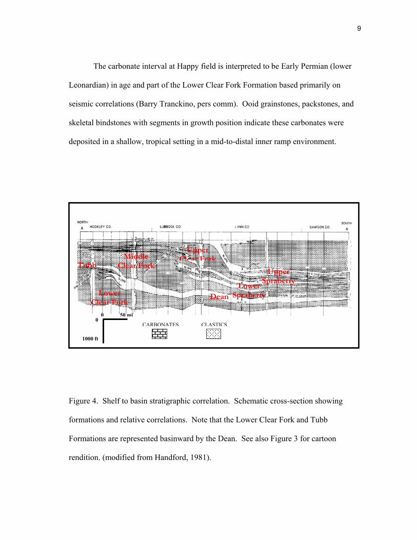
The carbonate interval at Happy field is interpreted to be Early Permian (lower
Leonardian) in age and part of the Lower Clear Fork Formation based primarily on
seismic correlations (Barry Tranckino, pers comm). Ooid grainstones, packstones, and
skeletal bindstones with segments in growth position indicate these carbonates were
deposited in a shallow, tropical setting in a mid-to-distal inner ramp environment.
Figure 4. Shelf to basin stratigraphic correlation. Schematic cross-section showing
formations and relative correlations. Note that the Lower Clear Fork and Tubb
Formations are represented basinward by the Dean. See also Figure 3 for cartoon
rendition. (modified from Handford, 1981).
LowerSpraberryDean
UpperSpraberry
UpperClear Fork
LowerClear Fork
TubbMiddle
Clear Fork
CARBONATES CLASTICS
0 50 mi0
1000 ft

10
PREVIOUS WORK
Happy Spraberry Field
Happy Spraberry field was discovered by Bennett Petroleum in 1988 on an
Ellenberger Formation recompletion target in the Lott 19 #1 well. After completing a
3D seismic survey in 1989, Bennett Petroleum and Torch Energy drilled six wells in the
John F. Lott Lease. Torch Operating Company acquired all production interests and
drilled nine more wells by 1992. Field unitization soon followed and a waterflood
program was implemented, converting several marginal-producing wells over to
injection wells. Production is currently at a 40 acre spacing (Hammel, 1996).
Studies on the field have been of special interest at Texas A&M University for
over 10 years because the availability of cores, core analyses, and borehole logs has
provided an exquisite data set for study. Work is still underway to determine
relationships between petrophysical and lithologic characteristics in order to find more
reliable ways to identify reservoir quality.
Hammel (1996) conducted the initial study on the field. He created a quality
classification scheme based on porosity-permeability paired values from core analyses.
He then compared quality from poro-perm pairs with thin section observations to find
lithologic proxies for reservoir quality. Finally, these proxies were placed in proper
stratigraphic architecture to enable predictive maps of reservoir quality to be
constructed.
Roy (1998) made a similar study on half of the cores in the field. His findings on
reservoir quality were consistent with Hammel’s (1996) and a better understanding of

11
the stratigraphic architecture of flow units was gained.
Mercury Injection Capillary Pressure (MICP) data from Happy field has also
been studied by Ahr. MICP data yields information on pore throat size distributions
within a sample. This data has also been studied to determine how pores are in
communication in 3D. Waterflood programs have been implemented to enhance
recovery and increase production in marginal fields. These studies have helped to
provide information for improved waterflood programs.
Petrographic Image Analysis (PIA)
Digital image analysis is not new. It is simply the capturing of digital images
and then analyzing image properties. This has become common practice in recent years
following the appearance of high-speed desktop computers. Image acquisition and
analysis software is now used by geoscientists in a wide variety of petrographic
applications including textural, mineralogical, fabric, and porosity analyses.
Comparatively more work has been done on siliciclastic rocks than on
carbonates. A pioneer in this effort is Robert Ehrlich at the University of South
Carolina. His work helped identify pore characteristics in siliciclastic rocks by means of
digital images and a software platform (Ehrlich et al., 1984; 1991a). He and others have
done extensive work utilizing petrographic image analysis to relate pore and pore throat
geometry to capillary pressure measurements (McCreesh et al., 1991). Work was also
done on forward modeling of permeability from porosity values attained from PIA
(Ehrlich, 1991b).

12
Image analysis on carbonates is rare compared to the volume of work done on
siliciclastics. Several studies examined cathodoluminescent-zoned cements using PIA in
an effort to delineate cementation events. This was helpful in determining porosity
changes before and after hydrocarbon migration (Dorobek et al., 1987). Currently, a
commercial laboratory in the England (Cambridge Carbonates Ltd.) performs this type
of analysis as part of reservoir evaluations. PIA has also been used to identify and
digitally remove generations of cementation. With this, it was possible to determine
which porosity generation was responsible for the most significant pore destruction and
thus to identify the “porosity killer” cement (Mowers and Budd, 1996).
Anselmetti et al., (1998) measured pore geometry in a number of modern
carbonate rocks from the Bahama Banks to the Middle East. He analyzed porosity with
an “order of magnitude” approach. Images of photomicrographs and scanning electron
micrographs were analyzed with PIA. Pore dimensions range from less than 1 micron to
a millimeter and cover three orders of magnitude. His study was of value because it
focused on segmenting porosity into micro- and macroscopic components. This method
established which population of pores was responsible for and contributed to overall
reservoir quality. It also provided a rough parallel for this study. However, he did not
discuss the implications of pore type, nor did he examine his results in a stratigraphic
context.
Nature of This Study
This study differs from other image analysis studies in several ways. Most image

13
analysis has been performed on porosity of siliciclastic samples because purely
intergranular porosity is much easier to characterize than the multiple pore types that
occur in carbonates. Siliciclastic porosity is, in essence, a negative image of the adjacent
quartz grains. Carbonate pores form by three end member genetic processes and are
certainly more diverse than their siliciclastic counterparts. Carbonate pores may reflect
multiple episodes of diagenetic alteration; therefore their origin and geometry is not
always simple to interpret
A study of 52 thin sections of carbonate pores and 5 cores from Happy field was
done to determine relationships between pore characteristics and reservoir quality to
show that pore size, shape, and abundance are useful indicators of relative quality in
reservoir flow units.

14
METHODS
Pore properties including area (size), aspect ratio and roundness (shape) and
abundance, were measured by petrographic image analysis (PIA). Pore facies were
developed from pore data and ranked from best to worst according to petrophysical
attributes and pore implications on reservoir quality. Higher poro-perm pairs were
associated with better quality pore facies than were lower poro-perm pairs. These
differences are the basis for the quality classification system.
Lithological Study
Approximately 700 feet of slabbed core from five wells was examined under
binocular microscope. Core was described in detail for depositional texture, constituent
composition, porosity percent and type, pore-filling cements, and sedimentary structures
(Appendix A). Rock types were classified by depositional texture following Dunham’s
(1962) classification system. These descriptions provided the data for identification of
depositional facies and development of a depositional model for the Happy field
carbonates.
Core Laboratories performed core analyses (SCAL) on cores from the John F.
Lott lease wells; data include porosity, permeability, saturation, and grain density. Core
porosity from the SCAL data was compared to porosity values calculated from borehole
logs, from visual estimates in petrographic studies, and from petrographic image
analysis. Porosity values were calculated from neutron and density logs. Values were
calculated according to Asquith (1997) using neutron-density porosity cross-plot and

15
drilling mud corrections. Core data of porosity and permeability was graphed to
determine if a linear relationship between the two values existed.
Borehole Logs
Wireline logs used in the study include gamma ray, spontaneous potential,
resistivity, induction, and neutron-density logs. Gamma ray and SP logs were examined
and correlated with rock type. Lithofacies were found to exhibit log signatures that were
correlatable across the field.
Thin-Section Petrography
Thin sections used in studies done by Hammel (1996) and Roy (1998) were
examined using standard petrographic methods. Counts of pore size and shape were
made at 200 points on each thin section. In all, 52 stained samples from Lott 19 #4 and
Lott 19 #7 wells were studied under plane light. Thin sections were examined to
identify visible porosity, grains, cements, and matrix (lime mud or shale) (Appendix B).
A micrometer ocular was used to measure pore size. Pore area was calculated from
multiplying length and width pore dimensions. Pores were classified using the genetic
classification scheme formulated by Ahr (Ahr and Hammel, 1999). Genetic categories
were subsequently compared with size data to determine the geological relationship
between pore geometry and total, visible porosity as a percentage of total thin section
area. Estimates of total visible porosity were compared with total core porosity from the
same depth to test for the reliability of visual, 2D estimates as predictors of volumetric,

16
3D porosity. High correspondence of those data indicate that visible porosity of a 2D
thin section can be used as a predictor for total, 3D pore volume of a rock.
Petrographic Image Analysis (PIA)
Equipment
The image analysis system consists of a Sony DXC-290, CCD color video
camera mounted on a Zeiss petrographic microscope. Images were captured by the
camera and then relayed to a PC equipped with a graphics card and the commercial
image analysis software program Image Pro Plus. Images viewed through the
microscope were focused for viewing and subsequent capture by the image analysis
system (Figure 5). Magnification, light source, light intensity, and light polarity were
standardized so that measurement techniques were comparable on all thin sections
sampled. Images were then saved as .tif image files for later analyses.
Calibration
A calibration slide (Figure 6) was viewed under various magnifications, and the
best results for a wide range of measurement sizes was found to be 12.5 diameters. This
magnification was achieved with a 2.5 X objective and a 5 X phototube assembly. This
magnification was solely used for this study because the “order of magnitude approach”
of Anselmetti et al., (1998) would not produce specific numerical values for
measurements of pore geometry. The field of view at 12.5 X magnification is large
enough to accommodate entire pores of the size common to rocks in this study. Also, at

17
12.5X, the smallest, practical size for pore measurements was found to be about 100
square microns.
Figure 5. Screen capture of Image Pro Plus image analysis software. This is a screen
capture in color-segmentation mode. The cursor was placed on any pore (blue). Pixels
of that blue color as well as other pixels of that color in the image (other pores) were
then identified. This process was repeated until the porosity could be repeatedly
identified with reproducible results.

18
Figure 6. Calibration slide image. This is an image in .tif format showing the
calibration slide. The scale bar is 1 mm or 1000 microns in length. This image provided
a specific reference length to calibrate the software for subsequent pore measurements to
be taken. Image is not to scale.
Sampling
Fields of view from thin sections were chosen on the basis of ranges of visible
porosity. Thin sections were studied systematically by tracking in an X-pattern (Figure
7). This method made obtaining measurements more consistent. Ten images were
captured from each thin-section. The porosity value of each image was determined and
average porosity was tabulated for each of the ten images. The image with the porosity
value that most closely corresponded with the average porosity for the entire thin section
was then analyzed in detail, as it was the most representative sample image of the thin
section.

19
Figure 7. Schematic of thin-section sampling. 10 images per thin section were obtained
using the above procedure.
Measurements
Pores were identified by a process of color segmentation (Figure 5). By placing
the cursor on a pore, that pore color, and all pores of that color were electronically
identified and tallied. This procedure was repeated until all pores had been accurately
identified.
Measurements that would allow for quantitative analysis of carbonate pores were
selected after all pores were identified. The size, shape, abundance (total), and
frequency distribution of pores were logged (Figure 8). Pore area (size) was given in
square microns for each pore. The total porosity seen in an image (abundance) is the
ratio of the sum of all pore areas to the area of the entire image. This is also referred to
as Total Optical Porosity (Ehrlich et al., 1984). Frequency is the distribution of pore
sizes that comprise the total porosity.
12 3
4 5
678
910
Lott 19 #44932.6’

20
Pore shape was determined by measuring the aspect ratio and roundness factor
(Table 1). The aspect ratio measurement is equal to the ratio between the major axis and
minor axis of the object; it is a measure of pore elongation (Figure 8). The roundness of
an image was calculated using the formula perimeter2 / 4 π a, where a is equal to pore
area. An object with an aspect ratio of 1-1.5 is considered equidimensional.
Equidimensional shapes in this study were either circles or squares. An object was
considered square if it was equidimensional and had a roundness factor above 3. An
equidimensional shape with a roundness factor of less than 3 was interpreted as a circle.
An object with an aspect ratio above 1.5 was considered elongate. An elongate and
round shape was interpreted as an ellipse; elongate and non-round as a rectangle.
Table 1. Shape interpretation table. Combinations of aspect ratio and roundness data
were used to interpret geometrical shapes to assign to pore types.
Aspect Ratio (length/width)
Roundness (perimeter2/ 4*B*area)
Shape (geometric equivalent)
LOW (1-1.5) ROUND (1.0-3.0) CIRCLE
LOW (1-1.5) Non-ROUND (3.0+) SQUARE
HIGH (1.5+) ROUND (1.0-3.0) ELLIPSE
HIGH (1.5+) Non-ROUND (3.0+) RECTANGLE
4 π area)

21
Figure 8. Measurement window. Measurements were selected according to purpose.
Shown are those used in this study.
Auto-Classification
The porosity in the image was then classified into size and shape categories. The
number of categories selected was determined by the number of pore types present in the
sample (Figure 9). Grouped categories based on size and shape were useful in
determining pore origin. This is significant because it indicates that pore geometry and
pore origin may be related. Specific pore types were auto-classified such that the

22
average size and shape of that pore type was measured automatically. The total
abundance of porosity as well as frequency distribution of pore types were also
determined automatically by Image Pro Plus.
Figure 9. Auto classification window. Pores were classified according to size, aspect
ratio, and roundness. In this case the pores were classified into 4 categories and then
iterations were performed to determine statistics of each category.

23
RESULTS
Lithofacies were identified based on constituent composition, depositional
texture, and sedimentary structures. Lithofacies were then correlated across the field
using wireline logs and core descriptions. The field-wide distribution of lithofacies
enabled a depositional model to be developed for Happy field. Lithofacies descriptions
and the depositional model incorporate previous work by Hammel (1996).
Lithofacies
There are 5 lithofacies present at Happy field; oolitic skeletal grainstones and
packstones, floatstones, rudstones, in situ Tubiphytes bindstones, and siliciclastic
sediments. The principal reservoir rock is the oolitic skeletal grainstone packstone
lithofacies.
Oolitic Skeletal Grainstones and Packstones
The most abundant lithofacies at Happy field consists of oolitic skeletal
grainstones and packstones (Figure 10). The facies is present in all wells and ranges in
thickness from 15 to 50 feet across the field. Core segments of these rocks are typically
pale gray to light tan in color. Oil staining is also common and may alter the color to
dark tan or brown. Ooids and skeletal allochems are commonly present only as molds
after having been removed by dissolution diagenesis. Sedimentary structures are present
but are obscure because there is little contrast in grain size or grain color to distinguish

24
them. Faint crossbedding is visible in some core intervals. This lithofacies is interpreted
to have been deposited in a moderately agitated, shallow marine, tropical environment.
Figure 10. Core photos of oolitic and skeletal grainstone. Core samples are from 4933’
and 4937’, Lott 19 #4 well. A) Skeletal and oolitic grainstone. Note well-developed
skel-moldic porosity (arrow) approaching 1 cm in length. B) Oil stained oolitic
grainstone. Water applied for photographing (arrow) has beaded due to residual oil
saturation.
A B
1 cm1 cm

25
Floatstones
Floatstones occur as time-equivalent deposits of the oolitic grainstone facies.
Rocks are composed of a silty, lime-mud matrix with large, isolated clasts (Figure 11).
The matrix is typically dark gray to black in color and may contain minor amounts (less
than 10%) of marine phreatic, calcite cement. Clasts are composed of oolitic facies or
skeletal fragments and may reach 5 cm in diameter. The floatstone lithofacies is
interpreted to have been deposited as reworked material adjacent to the oolitic and
skeletal source. The muddy matrix indicates less winnowing, probably owing to the
rubble beds having been partly sheltered in the lee of the skeletal and oolitic shoals.
Figure 11. Core photo of floatstone. Core sample is from 4981’, Lott 19 #4 well.
Isolated clasts of oolitic facies (A) and crinoid fragment (B) in a muddy matrix. Clasts
exhibit crude imbricated fabric near the right portion of the photo.
1 cm
A
B

26
Rudstones
Rudstones are interpreted to have been deposited closer to the organic buildup
sources (“reefs”) because these rocks contain larger clasts and less fine matrix.
Rudstones are clast-supported rocks in which clasts are typically composed of the oolitic
facies or reefy, rubble material. Clasts may reach a size of 10 cm in diameter. Skeletal
fragments are also commonly found whole (Figure 12) further supporting the
interpretation that rudstones were deposited close to their source and underwent little
transportation and abrasion. This lithofacies is interpreted to have been deposited
adjacent to the oolitic grainstone facies in a low, or saddle between the two grainstone
pods that was filled with rudstone debris shed off of the flanks of the buildup.
Figure 12. Core photo of rudstone. Core sample is from 4963’, Lott 19 #4 well. Note
brecciated, poorly sorted texture. Clasts are composed of bindstone reef rubble and are
larger and more abundant than clasts in the floatstone facies.
1 cm
27
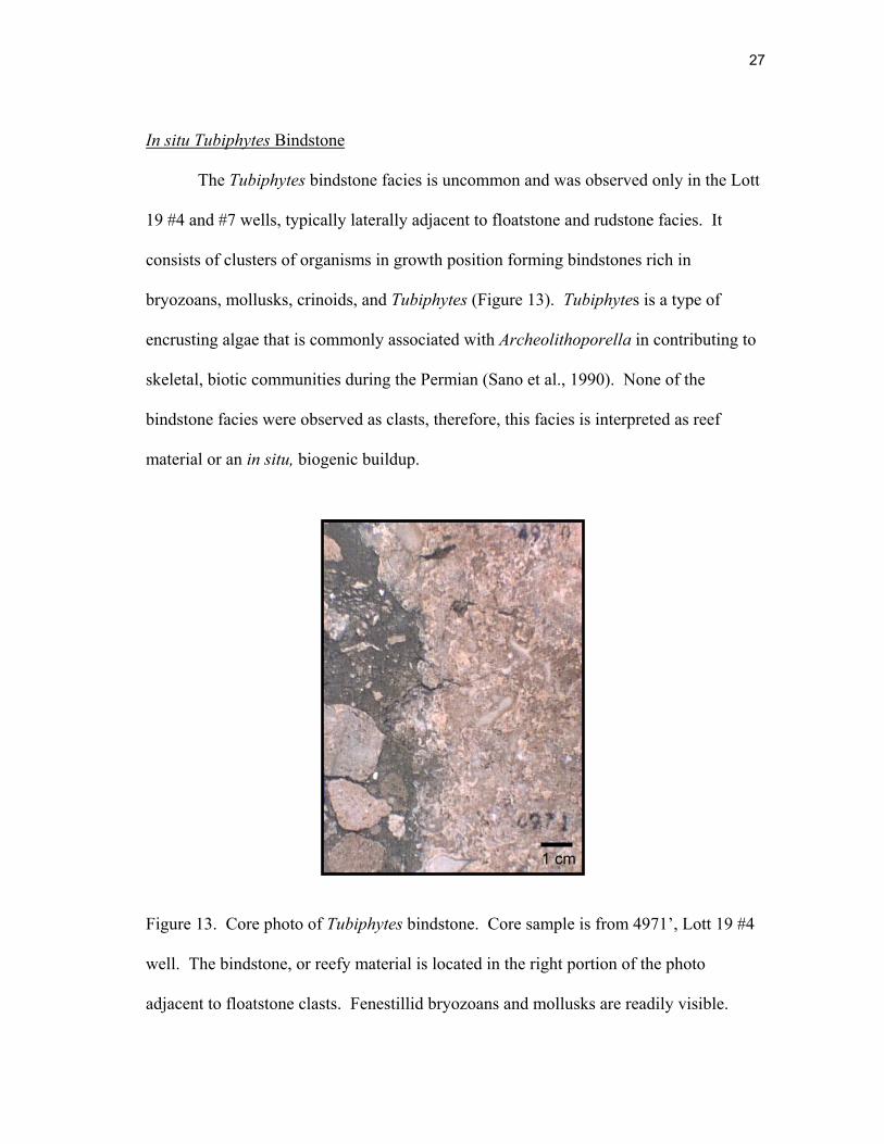
In situ Tubiphytes Bindstone
The Tubiphytes bindstone facies is uncommon and was observed only in the Lott
19 #4 and #7 wells, typically laterally adjacent to floatstone and rudstone facies. It
consists of clusters of organisms in growth position forming bindstones rich in
bryozoans, mollusks, crinoids, and Tubiphytes (Figure 13). Tubiphytes is a type of
encrusting algae that is commonly associated with Archeolithoporella in contributing to
skeletal, biotic communities during the Permian (Sano et al., 1990). None of the
bindstone facies were observed as clasts, therefore, this facies is interpreted as reef
material or an in situ, biogenic buildup.
Figure 13. Core photo of Tubiphytes bindstone. Core sample is from 4971’, Lott 19 #4
well. The bindstone, or reefy material is located in the right portion of the photo
adjacent to floatstone clasts. Fenestillid bryozoans and mollusks are readily visible.
1 cm
28
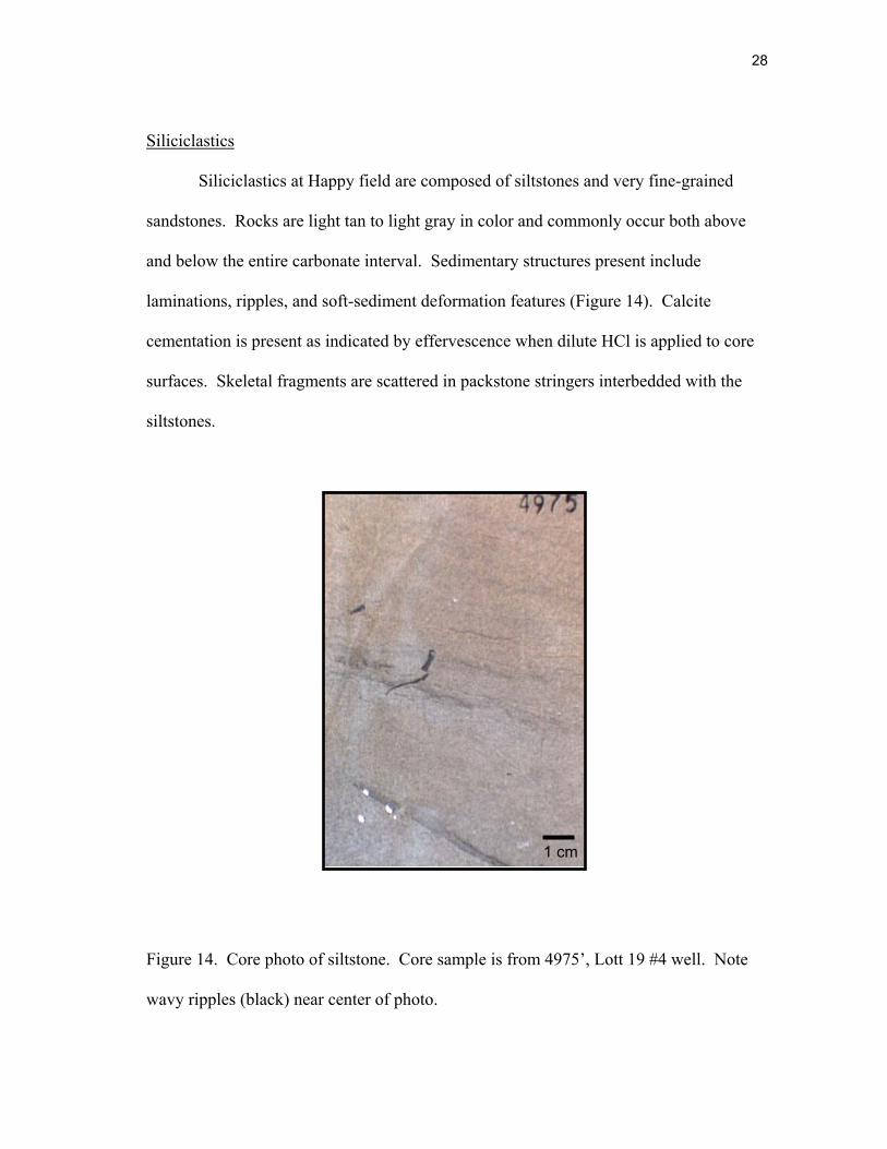
Siliciclastics
Siliciclastics at Happy field are composed of siltstones and very fine-grained
sandstones. Rocks are light tan to light gray in color and commonly occur both above
and below the entire carbonate interval. Sedimentary structures present include
laminations, ripples, and soft-sediment deformation features (Figure 14). Calcite
cementation is present as indicated by effervescence when dilute HCl is applied to core
surfaces. Skeletal fragments are scattered in packstone stringers interbedded with the
siltstones.
Figure 14. Core photo of siltstone. Core sample is from 4975’, Lott 19 #4 well. Note
wavy ripples (black) near center of photo.
1 cm

29
Depositional Environment
A depositional model for Happy field was developed using lithologic
characteristics determined from core descriptions and thin-section petrography, as well
as previous work by Hammel (1996). The rocks described and facies interpreted
represent deposition in a shallow marine setting. The carbonate rocks present at Happy
field were deposited on a distally steepened ramp as an oolitic sand and skeletal buildup
shoal complex. Siltstones and very fine-grained sandstones were deposited in an open
marine setting as well, but were not the primary focus of this study.
The oolitic and skeletal grainstone and packstone facies is commonly found near
the top of the carbonate section at Happy field. Ooids, skeletal fragments, and peloids
are well rounded and well sorted. Average ooid grain diameter is 200-300 microns. The
lack of matrix and presence of coated grains indicate deposition in shallow, agitated
water. Evidence also suggests that the environment was well worked by tidal currents
and was within fair-weather wave base. The sand waves represent mobile substrate
similar to the oolite shoals of the St. Louis Formation (Mississippian) as described by
Parham and Sutterlin (1994). Because this lithofacies is present in all cores at
approximately the same depth, it is suggested that the oolitic sand wave complex is
laterally continuous within the limits of Happy field.
The lithofacies of the rudstones, floatstones, and in situ Tubiphytes bindstones
represent environments adjacent to the oolite shoals. The in situ Tubiphytes bindstone is
a reefal facies of encrusting calcareous algae and bryozoans which form the binding
framework. The rudstones and floatstones represent material shed off of the buildups.

30
This shedding was a result of instability as wave energy, storm activity, and normal
breakdown eroded the buildups. Rudstones are interpreted to have been deposited in
comparatively higher energy environments than floatstones. The rudstones contain
larger intraclasts, less matrix, and were, therefore, deposited more proximal to the
buildups than floatstones. The presence of coated grains and photosynthetic, binding
organisms indicate shallow, tropical water that was well agitated and within fair weather
wavebase and tidal currents. Sedimentary structures in the oolitic sand waves are
consistent with deposition within a mobile substrate. Boundstones are evidence that
biogenic buildups were able to establish themselves on the current-swept seabed. These
buildups may have developed on subtle, structurally controlled, bathymetric features.
Log Analysis
Electric logs were available for the wells studied. Available were Gamma Ray (GR),
Spontaneous Potential (SP), Neutron Porosity (NP), Density Porosity (DP), and
Resistivity (R). GR, NP, DP, and R responses were observed to find log “signatures”
that correspond to lithofacies identified in cores. It was then possible to identify and
correlate lithofacies across the field with well logs where core control was absent.
GR log measures radioactivity in the borehole. Radioactive particles are relatively
more abundant in clay-sized detrital material, so this is an indicator of the presence of a
muddy matrix, be it siliciclastic shale or carbonate mudstone. The oolitic grainstone
facies, which is close to matrix-free, has a GR response of less than 20 API units, or

31
what would be termed “clean”. Other carbonate lithofacies, such as rudstones and
floatstones contain more carbonate mud and reflect higher GR counts.
Porosity logs may be useful in identifying porous and non-porous intervals in the
various lithofacies. Log derived porosity was calculated from NP and DP logs (Figure
15) and compared to total porosity values obtained from alternate methods. Porosity in
Happy field varies from 10%-26%. Generally, oolitic grainstone porosity varies
between 20%-26%, rudstones and bindstones 12%-20 %, and floatstones and
siliciclastics less than 12%. Though not shown, resistivity response across the carbonate
interval must also be noted. R response measures how resistive rock is to electrical
current and indicates whether a rock is saturated with hydrocarbons or water. The
productive oolitic grainstone lithofacies is also apparent on the R response and exhibits
counts in excess of 100 ohm/m, which is typical of oil-bearing zones. Non-reservoir
rocks, such as floatstones and siliciclastics, register responses of less than 10 ohm/m,
thus indicating they are not hydrocarbon bearing zones.
Core Analysis
Core from five wells used in the study underwent special core analysis performed by
Core Laboratories. Porosity and permeability values were measured at one-foot
intervals, and were graphed on semi-log plots in order to determine the relationship
between the two data sets. This is useful for calculating permeability from porosity
values that have been obtained by methods other than special core analysis, such as
wireline porosity logs. Higher poro-perm pairs indicate higher reservoir quality.

32
Figure 15. Type log for Happy field, Lott 19 #4. Note the “clean” GR response and the
serrate NP and DP log responses to the oolitic grainstone interval. The grainstone
interval was easily correlated across the field.
Gamma Ray Porosity Log 0 API 100 30 -10
Density
NeutronGamma Ray
Shaly Siltstone
Oolitic Grainstone
Skeletal Rudstone
Floatstone
Shaly Siltstone

33
Thin-Section Petrography
Thin sections were examined to measure pore size, shape, frequency, and
abundance. Repeat measurements were made using Image Pro Plus software and the
camera apparatus described in the methods chapter. The repeat measurements were
made to determine if image analysis techniques could reproduce measurements obtained
by traditional optical petrography.
Pore Measurements
A standard 200 point-count analysis was performed on the thin section samples
to determine constituent percentages and to obtain pore data. Thin sections were
analyzed and each count was tallied as porosity, grain, cement, quartz, or matrix. The
percent of each constituent was then determined (Appendix B). Total porosity from
petrography was compared with total porosity obtained from core analyses, log-derived
porosity, and PIA porosity. This was necessary to establish that measured values of
porosity from standard petrography were in agreement with values of porosity obtained
by other methods. Major and minor axis dimensions were measured on counted pores to
provide an estimate of pore size. Pore size was represented as pore area. Pore shape
was estimated by eye as circle, square, ellipse, or rectangle. Finally, the pores were
classified using the genetic system developed by Ahr and students. This genetic
classification system allows for pores to be placed in the context of depositional and
diagenetic processes, so that various pore types can be set in a larger context of the
stratigraphic architecture at the field scale.

34
Genetic Classification of Carbonate Pores
Several classification systems for carbonate porosity have been developed, such
as those developed by Archie (1952) and Choquette and Pray (1970). The Archie (1952)
classification system is based on the texture of rock matrix, visible pore structure, and
typical petrophysical behavior that would be associated with the rock. The system
developed by Choquette and Pray (1970) classifies pores on the basis of whether they
are fabric selective or not. It includes subsidiary descriptive sections that relate to
diagenetic alteration as well as additional size modifiers. The scheme developed by
Lucia (1983) classifies porosity as either interparticale or vuggy. This takes into account
that interparticle porosity and vuggy porosity have vastly different petrophysical
properties. Vugs were then further classified as touching or non-touching vugs.
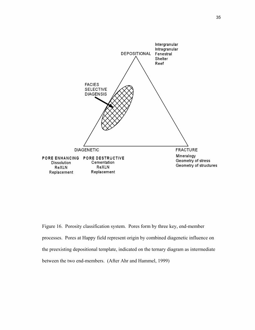
Carbonate pores are the result of three end-member processes- diagenetic,
depositional, and fracture (Ahr and Hammel, 1999). No material fractures were
observed at Happy field. Unaltered depositional pores are rare, but do exist in the form
of intraskeletal pores within bryozoans. The intraskeletal pores do not contribute to
overall, effective porosity. Pores at Happy field are primarily the result of a diagenetic
overprint on a preexisting depositional texture present in specific lithofacies; i.e. oolitic
grain-moldic porosity present in an oolitic grainstone or packstone. Accordingly, such
pores would exist in an intermediate position between the diagentic and depositional
end-members of the ternary diagram (Figure 16).
35
Figure 16. Porosity classification system. Pores form by three key, end-member
processes. Pores at Happy field represent origin by combined diagenetic influence on
the preexisting depositional template, indicated on the ternary diagram as intermediate
between the two end-members. (After Ahr and Hammel, 1999)

36
Pore Types
Grain Moldic (M) and Incomplete Moldic (IM)
Molds and incomplete molds formed from the diagenetic dissolution of
metastable grains. Molds are typically of ooids and skeletal fragments. Moldic pores
exhibit sharp, distinctive outlines of leached grains, while incomplete moldic pore
boundaries are less distinctive and adjacent to recrystallized remnants of the original
grain. Moldic and incomplete moldic pores (Figure 17) dominate the oolitic skeletal
grainstone packstone facies and are the most significant contributors to overall pore
volume in the field.
Figure 17. Photomicrographs of moldic and incomplete moldic pores. A) Sample is
from Lott 19 #4 well, 4949.3’. Complete dissolution of ooid grains has resulted in well-
defined pore areas. B) Sample is from Lott 19 #7 well, 4954.7’. Incomplete dissolution
of ooids and skeletal grains has left grains partially intact. Scalebar = 100 microns.
A B
37
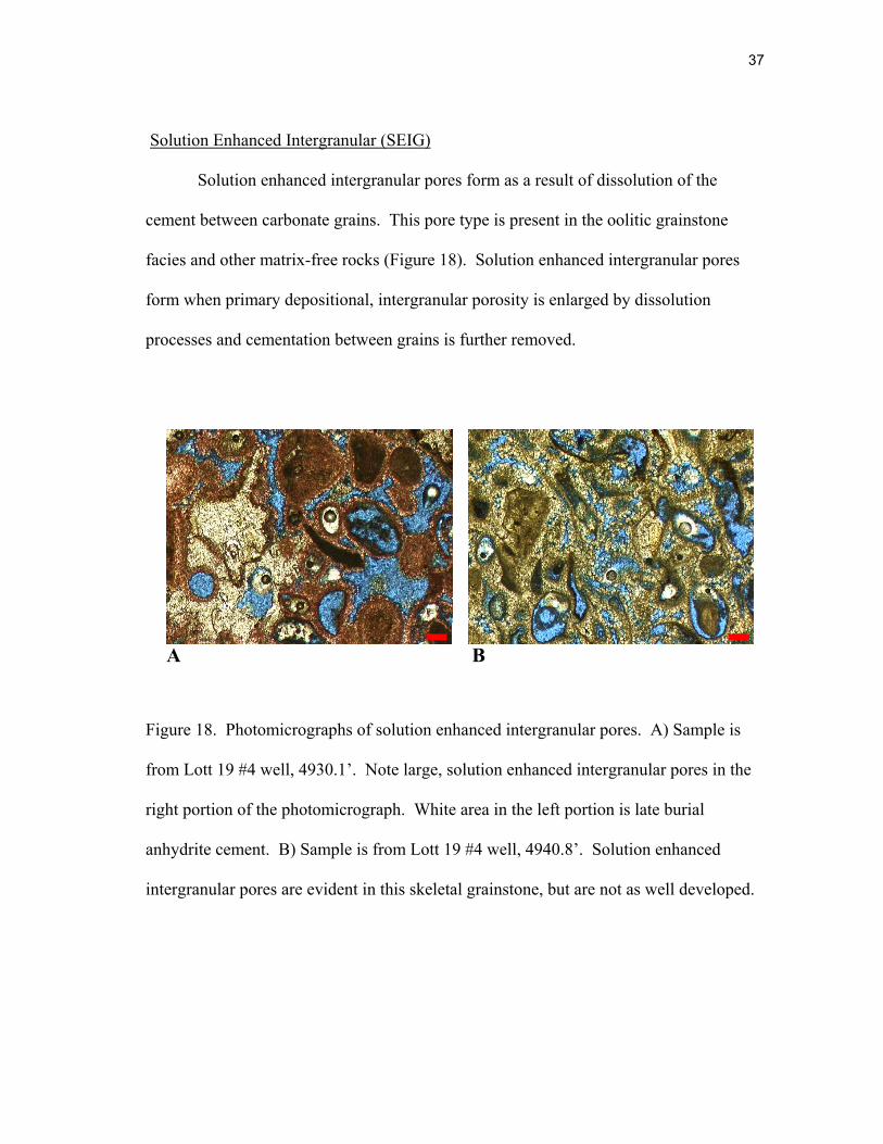
Solution Enhanced Intergranular (SEIG)
Solution enhanced intergranular pores form as a result of dissolution of the
cement between carbonate grains. This pore type is present in the oolitic grainstone
facies and other matrix-free rocks (Figure 18). Solution enhanced intergranular pores
form when primary depositional, intergranular porosity is enlarged by dissolution
processes and cementation between grains is further removed.
Figure 18. Photomicrographs of solution enhanced intergranular pores. A) Sample is
from Lott 19 #4 well, 4930.1’. Note large, solution enhanced intergranular pores in the
right portion of the photomicrograph. White area in the left portion is late burial
anhydrite cement. B) Sample is from Lott 19 #4 well, 4940.8’. Solution enhanced
intergranular pores are evident in this skeletal grainstone, but are not as well developed.
A B
38
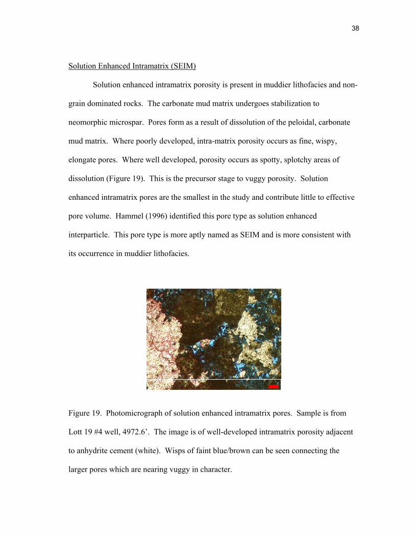
Solution Enhanced Intramatrix (SEIM)
Solution enhanced intramatrix porosity is present in muddier lithofacies and non-
grain dominated rocks. The carbonate mud matrix undergoes stabilization to
neomorphic microspar. Pores form as a result of dissolution of the peloidal, carbonate
mud matrix. Where poorly developed, intra-matrix porosity occurs as fine, wispy,
elongate pores. Where well developed, porosity occurs as spotty, splotchy areas of
dissolution (Figure 19). This is the precursor stage to vuggy porosity. Solution
enhanced intramatrix pores are the smallest in the study and contribute little to effective
pore volume. Hammel (1996) identified this pore type as solution enhanced
interparticle. This pore type is more aptly named as SEIM and is more consistent with
its occurrence in muddier lithofacies.
Figure 19. Photomicrograph of solution enhanced intramatrix pores. Sample is from
Lott 19 #4 well, 4972.6’. The image is of well-developed intramatrix porosity adjacent
to anhydrite cement (white). Wisps of faint blue/brown can be seen connecting the
larger pores which are nearing vuggy in character.
39
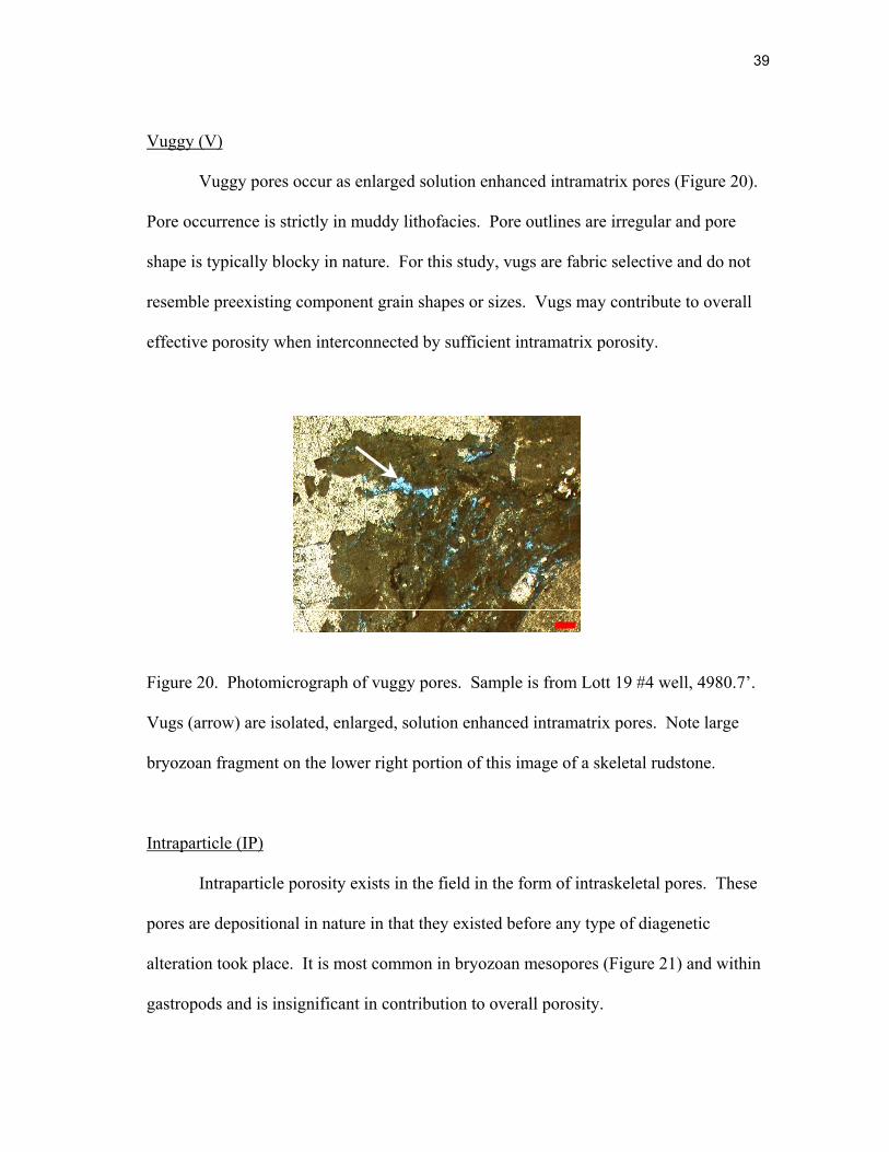
Vuggy (V)
Vuggy pores occur as enlarged solution enhanced intramatrix pores (Figure 20).
Pore occurrence is strictly in muddy lithofacies. Pore outlines are irregular and pore
shape is typically blocky in nature. For this study, vugs are fabric selective and do not
resemble preexisting component grain shapes or sizes. Vugs may contribute to overall
effective porosity when interconnected by sufficient intramatrix porosity.
Figure 20. Photomicrograph of vuggy pores. Sample is from Lott 19 #4 well, 4980.7’.
Vugs (arrow) are isolated, enlarged, solution enhanced intramatrix pores. Note large
bryozoan fragment on the lower right portion of this image of a skeletal rudstone.
Intraparticle (IP)
Intraparticle porosity exists in the field in the form of intraskeletal pores. These
pores are depositional in nature in that they existed before any type of diagenetic
alteration took place. It is most common in bryozoan mesopores (Figure 21) and within
gastropods and is insignificant in contribution to overall porosity.
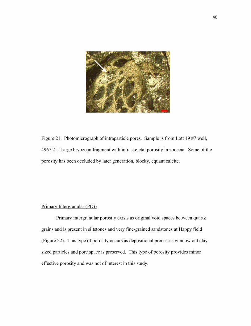
40
Figure 21. Photomicrograph of intraparticle pores. Sample is from Lott 19 #7 well,
4967.2’. Large bryozoan fragment with intraskeletal porosity in zooecia. Some of the
porosity has been occluded by later generation, blocky, equant calcite.
Primary Intergranular (PIG)
Primary intergranular porosity exists as original void spaces between quartz
grains and is present in siltstones and very fine-grained sandstones at Happy field
(Figure 22). This type of porosity occurs as depositional processes winnow out clay-
sized particles and pore space is preserved. This type of porosity provides minor
effective porosity and was not of interest in this study.

41
Figure 22. Photomicrograph of primary intergranular pores. Sample is from Lott 19 #7
well, 4991.6’. This siltstone retains original depositional porosity avoiding pore-
destructive cementation.
Petrographic Image Analysis (PIA)
Pores were identified and measured using petrographic image analysis. Pores
were classified according to geometry and the results indicate that pores that are
geometrically similar share the same origin. Image analysis data yielded information on
size, shape, frequency, and abundance of pores. Pore facies were then developed from
cumulative frequency histograms that incorporated all image analysis data. Pore facies
were ranked according to pore attributes (size, shape, and frequency) as well as
petrophysical properties (total porosity, or abundance, and permeability).

42
Data
Pore data was exported from Image Pro Plus to Excel spreadsheets (Table 2)
and processed. Pertinent information on pores was processed into frequency histograms
that incorporated the five data parameters; pore size, shape, type, frequency, and
abundance. Table 2 is the data measurements spreadsheet for Lott 19 #4, 4960.6’.
Table 2. Excel spreadsheet of pore data. Interpretations of shape were made, the
remaining data was utilized in the histograms.
This sample is a skeletal packstone with complete and incomplete grain moldic
porosity. Molds are mainly leached skeletal fragments (Figure 23A). Porosity was
identified, categorized, and processed to obtain an image that showed pores after
classification (Figure 23B). Histograms of pore data (Figure 24) were made in order to
test for relationships between categories of pore data. Also, porosity abundance
obtained from image analysis data was compared to porosity values obtained by
alternate methods, including core analyses, thin-section petrography, and log derived
porosity.
Color Class # of Objects % of Objects Total Area % Area Red 1 74 36.633663 15460.354 3.9124074Blue 2 119 58.910892 61519.523 15.568172Tan 3 9 4.4554458 318182.28 80.519424
Color Mean Area Mean Aspect Ratio Mean Roundness Total Per Area % of Per AreaRed 208.92369 2.9071846 1.369861 0.00531575 3.9124069Blue 516.97076 1.54058217 1.4153757 0.02115234 15.568175Tan 35353.586 1.9445627 5.888195 0.10940105 80.519417
43
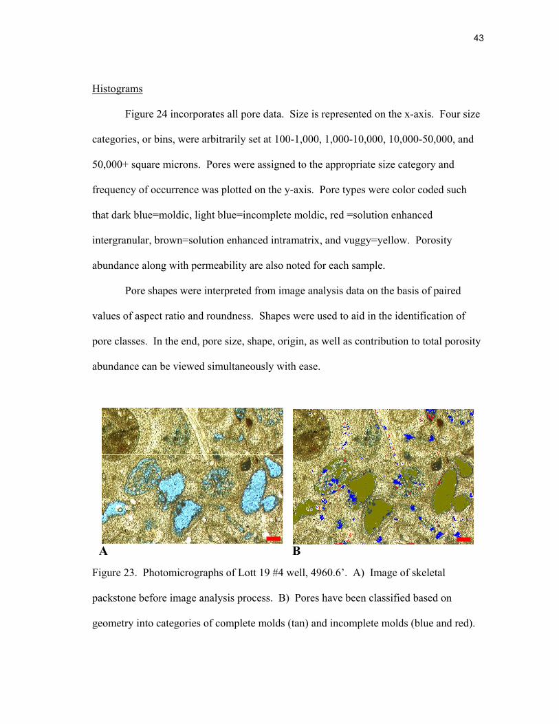
Histograms
Figure 24 incorporates all pore data. Size is represented on the x-axis. Four size
categories, or bins, were arbitrarily set at 100-1,000, 1,000-10,000, 10,000-50,000, and
50,000+ square microns. Pores were assigned to the appropriate size category and
frequency of occurrence was plotted on the y-axis. Pore types were color coded such
that dark blue=moldic, light blue=incomplete moldic, red =solution enhanced
intergranular, brown=solution enhanced intramatrix, and vuggy=yellow. Porosity
abundance along with permeability are also noted for each sample.
Pore shapes were interpreted from image analysis data on the basis of paired
values of aspect ratio and roundness. Shapes were used to aid in the identification of
pore classes. In the end, pore size, shape, origin, as well as contribution to total porosity
abundance can be viewed simultaneously with ease.
Figure 23. Photomicrographs of Lott 19 #4 well, 4960.6’. A) Image of skeletal
packstone before image analysis process. B) Pores have been classified based on
geometry into categories of complete molds (tan) and incomplete molds (blue and red).
A B

44
Figure 24. Frequency histogram of Lott 19 #4 well, 4960.6’. The histogram indicates
that the pore network is composed of large, rectangular, moldic pores and smaller,
incomplete moldic pores. The small, incomplete moldic pores do not provide adequate
connectivity, as indicated by only 4.3 md of permeability.

45
Pore facies are both fabric and facies selective. Trends in image analysis pore
data lead to the development of pore facies. A stratigraphic interval and petrographic
samples within that interval would share similar features in the cumulative frequency
histograms. The observations of patterns and trends in the histograms aided in the
identification and ranking of four pore facies present at Happy field.
Pore Facies
Four pore facies at Happy field were identified and ranked for reservoir quality.
Quality rankings are “best”, “intermediate”, and “worst”. The worst pore facies was
subdivided into two distinctive, identifiable pore facies.
The highest quality or “best” pore facies occur in the oolitic skeletal grainstones
at Happy field. Pore types are commonly moldic and solution enhanced intergranular
pores. An example of this pore facies is Lott 19 #4 well, 4923.8’ (Figure 25). The
facies has well developed, complete moldic porosity of ooids and skeletal fragments.
Solution enhanced intergranular porosity is also present. These pores are present as a
result of diagenetic leaching of grains and interstitial cement. The frequency histogram
for the sample (Figure 25) shows that large intergranular pores are present in
combination with large moldic pores. This pore facies typically has 15-25% porosity
and 12-25 md of permeability. An additional, representative sample of the oolitic
grainstone pore facies is present in the Lott 19 #7 well, 4978.9’, in the grainstone
interval (Figure 26).

46
Figure 25. Lott 19 #4 well, 4923.8’ photomicrographs and histogram. Note that
solution enhanced intergranular pores exist on two orders of magnitude of less than 1000
and larger than 10000 square microns.

47
Figure 26. Lott 19 #7, 4978.9’ photomicrographs and histogram. Large molds and
solution enhanced intergranular pores occupy 90% of total pore volume in the best pore
facies.

48
Intermediate quality pore facies are present in moderately cemented skeletal
grainstones and packstones. An example of this pore facies is present in the Lott 19 #7
well, 4981.2’ (Figure 27). Dominant pore types are incomplete moldic and solution
enhanced intergranular. A component of solution enhanced intergranular pores is also
common. Porosity is typically 15-25% and permeability ranges from 5-12 md.
The lowest quality pore facies is comprised of two sub-pore facies. The first
includes isolated molds that are present in highly cemented oolitic skeletal grainstones
(Figure 28). The leaching was only effective on metastable grains and little else
underwent micritization, stabilization, and neomorphism. As a result of this, the pores
are often isolated, unconnected, and would be classified as non-touching vugs (Lucia,
1983). Cumulative frequency histograms of this pore facies are typified by large
amounts of large molds, and less than 10% of any other pore type or size. Porosity
averages 10-14%, but may reach as high as 25%. Permeability is typically less than 5
md.
The overall lowest quality pore facies is present in silty, skeletal packstones,
siliciclastic siltstones, and rudstones (Figure 29). Typically, porosity is less than 10%
and permeability is less than 10 md. This rock type will have a considerable amount of
quartz present that aids in the large proportion of solution enhanced intergranular
porosity commonly found. Large, blocky vugs are also typical of this pore facies.
Hammel (1996) established a quality classification of flow units incorporating porosity
and permeability pairs. The relative quality of pore facies identified with PIA was
compared with intervals of Hammel’s “best, intermediate, and worst” and showed

49
Figure 27. Lott 19 #7, 4981.2’ photomicrographs and histogram. Intermediate pore
facies where incomplete moldic porosity dominates with occasional, minor complete
moldic. A component of solution enhanced intergranular porosity is also common.
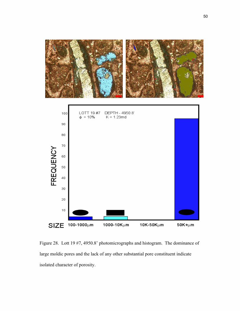
50
Figure 28. Lott 19 #7, 4950.8’ photomicrographs and histogram. The dominance of
large moldic pores and the lack of any other substantial pore constituent indicate
isolated character of porosity.

51
Figure 29. Lott 19 #4, 4971.4’ photomicrographs and histogram. The typical signature of
this pore facies was the combination of solution enhanced intramatrix and intergranular
pores. Blocky, vuggy porosity was also common.
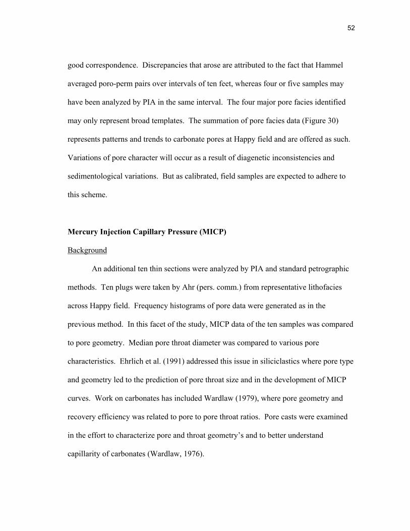
52
good correspondence. Discrepancies that arose are attributed to the fact that Hammel
averaged poro-perm pairs over intervals of ten feet, whereas four or five samples may
have been analyzed by PIA in the same interval. The four major pore facies identified
may only represent broad templates. The summation of pore facies data (Figure 30)
represents patterns and trends to carbonate pores at Happy field and are offered as such.
Variations of pore character will occur as a result of diagenetic inconsistencies and
sedimentological variations. But as calibrated, field samples are expected to adhere to
this scheme.
Mercury Injection Capillary Pressure (MICP)
Background
An additional ten thin sections were analyzed by PIA and standard petrographic
methods. Ten plugs were taken by Ahr (pers. comm.) from representative lithofacies
across Happy field. Frequency histograms of pore data were generated as in the
previous method. In this facet of the study, MICP data of the ten samples was compared
to pore geometry. Median pore throat diameter was compared to various pore
characteristics. Ehrlich et al. (1991) addressed this issue in siliciclastics where pore type
and geometry led to the prediction of pore throat size and in the development of MICP
curves. Work on carbonates has included Wardlaw (1979), where pore geometry and
recovery efficiency was related to pore to pore throat ratios. Pore casts were examined
in the effort to characterize pore and throat geometry’s and to better understand
capillarity of carbonates (Wardlaw, 1976).

53
The MICP portion of the study was concerned with determining if a relationship
existed between pore data obtained from PIA and median pore throat diameters from
MICP tests. Though different wells and depths were sampled compared to the pore
facies data, the ten samples were in accordance with the pore facies model already
established. Pore throat size frequency, median pore throat diameter, porosity, and
permeability of each sample was known from MICP analyses (Figure 31). MICP curves
also provide data on pore throats in that they are cumulative frequency plots of pore
throat size distribution.

54
Fig
ure
30.
Sum
mar
y of
PIA
dat
a. D
ata
sum
mat
ion
of th
e fo
ur p
ore
faci
es id
enti
fied
at H
appy
fie
ld in
clud
es p
ore
freq
uenc
y, b
in/s
ize,
sha
pe, t
ype,
as
wel
l as
poro
sity
and
per
mea
bili
ty in
terv
als
expe
cted
wit
h sp
ecif
ic p
ore
faci
es.

55
Figure 31. Pore throat size distribution. This plot shows the relative abundance of pore
throat sizes within this sample. As is evident by the spike, the majority of pore throat
diameters are approximately 10 microns in size.

56
DISCUSSION
This study focused on two main questions: 1) Can porosity values obtained from
image analysis accurately estimate porosity values from other methods, such as core
analyses, wireline logs, and standard petrographic analyses? and 2) Can pore data
obtained from petrographic image analysis serve as a rapid method to identify reservoir
quality, both with a pore facies model and MICP data?
Total Porosity
Reservoir quality depends on the relationship between porosity and permeability.
Typically, the most reliable measurements of porosity and permeability are made on core
samples. Alternatively, wireline log derived porosity may be related statistically to core
permeability. Close correlation between porosity and permeability measurements is
characteristic of a simple, intergranular porosity network. This simple pore network
does not exist at Happy field, which exhibits pores that have undergone extensive fabric-
selective diagenesis. Thus a close correlation of porosity and permeability values is also
nonexistent. Semi log plot of porosity vs. permeability shows poor correlation (Figure
32), suggesting predictions of permeability from total porosity values are unreliable.
This is a common predicament when dealing with carbonates that contain several pore
types and sizes and are not related to permeability by a simple, linear equation.
In order to find a method to relate porosity and permeability to reservoir quality,
values of porosity and permeability were paired for each sample and paired values were
grouped into highest, intermediate, and lowest combined values. These ranked porosity

57
and permeability values were used as reservoir quality indicators. Common pore
characteristics from PIA data were then determined for samples of equal quality. This
method established the pore facies model discussed in RESULTS (p. 45) where pore
attributes aid in the prediction of petrophysical behavior and reservoir quality. However,
porosity and permeability pairs can be related to specific lithofacies within the field, as
each lithofacies has a characteristic “porosity fingerprint”. This indicates that bracketed
values of porosity and permeability would be expected with certain rock types within the
field. As indicated by Figure 33, lihofacies with pore attributes in common plot as fields
of similar porosity and permeability values. For example, oolitic grainstones exhibit the
highest poro-perm values, and are the highest quality reservoir rocks in the field as a
result of the abundance and specific combinations of pore types and sizes.
Porosity values obtained by core analyses, standard petrographic methods, and
wireline logs were compared to values obtained from PIA. This was done by comparing
core porosity with porosity from standard petrographic analyses in order to compare
measured porosity values. The good correlation between core porosity and petrographic
porosity (Figure 34) indicates that porosity measured as 2D images corresponds well
with measured core porosity. Total porosity in each sample was determined by image
analyses and was compared with porosity obtained by standard petrographic methods.
This comparison established that porosity from standard petrography which is measured
across the entire thin section correlates well with PIA porosity which is obtained from a
series of points on each thin section sample. All image analysis measurements were
conducted using identical magnification for each pore size range. Figure 35 illustrates

58
Fig
ure
32.
Cor
e po
rosi
ty v
s. c
ore
perm
eabi
lity
. T
his
show
s to
tal p
oros
ity
mea
sure
d w
ith
all p
ore
type
s an
d
size
s in
clud
ed.
Cor
e φ
vs. C
ore
K
Cor
e φ
( %
)
Core K (md)
y =
.547
2x –
2.5
854
R2 =
.276
7

59
Fig
ure
33.
Cor
e po
rosi
ty v
s. c
ore
perm
eabi
lity
wit
h li
thof
acie
s. N
ote
that
sim
ilar
lith
ofac
ies
plot
in c
omm
on
fiel
ds w
here
ool
itic
gra
inst
ones
exh
ibit
the
high
est p
oro-
perm
pai
rs.
Cor
e φ
vs. C
ore
K
Cor
e φ
(%)
Core K (md)

60
Fig
ure
34.
Cor
e po
rosi
ty v
s. p
etro
grap
hic
poro
sity
.
Cor
e φ
vs. P
etro
grap
hic
φ
Cor
e φ
(%)
y =
1.0
99x
– .7
603
R2 =
.739
2Petrographic(%)

61
Fig
ure
35.
Pet
rogr
aphi
c po
rosi
ty b
y st
anda
rd m
etho
ds v
s. im
age
anal
ysis
por
osit
y. N
ote,
that
PIA
met
hods
typi
call
y un
dere
stim
ates
vis
ual p
oros
ity
betw
een
3-5%
.
P
etro
grap
hic
φ v
s. I
mag
e A
nal
ysis
φ
Pet
rogr
aph
ic φ
(%)
y =
.794
7x –
1.3
43
R2 =
.699
1ImageAnalysis(%)

62
the correlation between visual estimates of porosity from PIA and standard petrography.
As the graph suggests, PIA methods will typically underestimate total porosity as
compared to standard petrography. This may be explained by two reasons. The choice
of magnification for PIA has great bearing on the amount of porosity present in an
image. The porosity imaged and measured is dependent on the size of the field of view.
High magnification may focus on a single pore occupying the entire field of view
resulting in exaggeration of porosity measured. Magnification that is too low does not
identify small pores precisely and reliably resulting in porosity values less than expected.
The reliability of porosity values obtained from PIA as compared to porosity from core
analyses is shown in Figure 36. This plot shows that porosity percent from PIA
underestimates porosity from core analyses. However, the high correspondence between
data types suggests the method of determining porosity from PIA is relatively accurate,
and can serve as a simple transform to substitute for measured porosity in core analyses.
Wireline logs were analyzed to determine porosity. Neutron porosity and density
porosity logs were analyzed for porosity values and then a corrected porosity value was
determined using both curve values and depending on mud type (Asquith, 1997). Figure
37 shows this relationship. Again, porosity measurements from PIA typically
underestimate wireline log values of porosity.
Porosity obtained from all methods plotted against depth is shown in Figure 38.
The plot indicates that porosity obtained from PIA typically underestimates porosity
compared to porosity obtained by alternate methods. There is good agreement between
the porosity values and a similar trend of data points.

63
Fig
ure
36.
Cor
e po
rosi
ty v
s. im
age
anal
ysis
por
osit
y. T
his
plot
sho
ws
tota
l cor
e an
d P
IA p
oros
ity
whi
ch
incl
udes
all
por
e ty
pes
and
size
s.
C
ore
φ vs
. Im
age
An
alys
is φ
Cor
e φ
(%)
y =
.967
x –
2.83
41
R2 =
.672
ImageAnalysis(%)

64
Fig
ure
37.
Imag
e an
alys
is p
oros
ity
vs. w
irel
ine
log
poro
sity
. Im
age
anal
ysis
con
sist
entl
y un
dere
stim
ated
wir
elin
e lo
g po
rosi
ty b
y 2%
-4%
.
Imag
e A
nal
ysis
φ v
s. W
irel
ine
Log
φ
Imag
e A
nal
ysis
φ (%
)
y =
.409
4x –
11.
483
R2 =
.450
6WirelineLog(%)

65
Figure 38. Lott 19 #4 well porosity comparison. SCAL = core analyses, PET =
petrographic methods, PIA = petrographic image analysis, and LOG = log porosity. Log
and PIA porosity were commonly underestimated compared to core analyses values.
PHILott 19 #4
4900’
4925’
4950’
4975’
SCAL PHIPET PHIPIA PHILOG PHI
(%)
66
Pore Data and Pore Facies
The pore facies model that was developed in the previous chapter is based on
pore data from PIA as an indicator of reservoir quality. Pore data includes pore size,
shape, origin, frequency (relative abundance), and total abundance of porosity. The
purpose is to determine whether pore data provides a reliable classification system for
reservoir quality.
The pore facies model was developed from pore data obtained and interpreted
from PIA methods. That data enabled a classification system to be created. Pore facies
were then identified, classified, and ranked according to pore attributes and assessed as
to relative quality. This system was compared with Hammel’s (1996) method where
reservoir quality is based on paired values of porosity and permeability. For example,
high poro-perm paired values are indicative of high quality reservoir rocks and low poro-
perm paired values are indicative of low quality reservoir rock. His classification
scheme resulted in six quality ranks that include the entire range of permeability values
at Happy field. The 3D architecture of the flow units was then established within Happy
field. The architecture is illustrated in Figure 28 (Hammel, 1996) which shows flow
units that were identified by poro-perm pairs in well bores and then correlated across the
field.
Hammel’s (1996) work, however, did not include attributes and properties of
pores. Also, it failed to determine the correlation between porosity measurements
obtained by various methods, namely standard petrography and core analyses.
Furthermore, total porosity comparisons were not evaluated to determine trends in

67
porosity values obtained, nor was total porosity subdivided into pore components to
determine relation of pore data to reservoir quality. This study by contrast focuses on
determining whether image analysis could accurately measure total porosity for
comparison with porosity values measured by other techniques. These techniques
include core analyses, standard petrographic techniques, and determining porosity from
wireline log analysis. Also, this study focused on dissecting the entire porosity complex
into components of size, shape, origin, and relative abundance and then to utilize the
data in developing a reservoir quality classification system.
Figure 39 is the legend for Figure 40. Figure 40 is a stratigraphic cross-section
of Happy field showing the flow unit architecture based on reservoir quality by pore
facies model developed from PIA data (Figure 30). This was compared with the
findings of Hammel (1996), most notably, Figure 28, to compare high and low quality
intervals in both systems. Good correspondence between intervals of comparable
quality was observed throughout the field. For example, Hammel (1996) identified an
oolitic grainstone interval with high poro-perm pairs in the Lott 19 #4 well. The same
grainstone “sweetspot” was also identified by the pore facies model as a high quality
section and subsequent correlation of this interval across Happy field resulted in flow
unit architecture that was comparable to that of Hammel (1996). The detail of
Hammel’s (1996) study was not reached as his model was based on poro-perm values
from core analyses which were provided across a 1-foot interval. In this study, the
model was based on porosity data from thin-section samples which were, on average,
taken across 5-foot intervals.
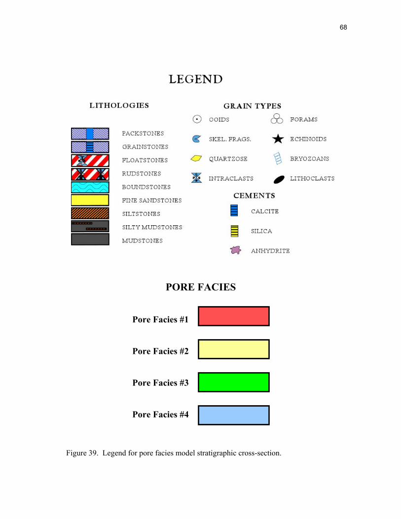
68
Figure 39. Legend for pore facies model stratigraphic cross-section.
PORE FACIES
Pore Facies #1
Pore Facies #2
Pore Facies #3
Pore Facies #4

69
Figure 40. Stratigraphic cross section incorporating pore facies model. Shown is a
stratigraphic cross section transecting southwest to northeast. The lithologic well logs
show rock type, primary grain constituents, and cements. The intervals of pore facies
architecture has been color-coded consistent with the pore facies model summarized on
page 54. The highest reservoir quality interval is associated with pore facies #1 (red)
which is present in the oolitic grainstone. This interval is suggested to increase in
thickness towards the northeast. Also note that the producing interval of pore facies #1
and #2 are typically bounded by non-productive, low quality reservoir rocks of the other
pore facies.
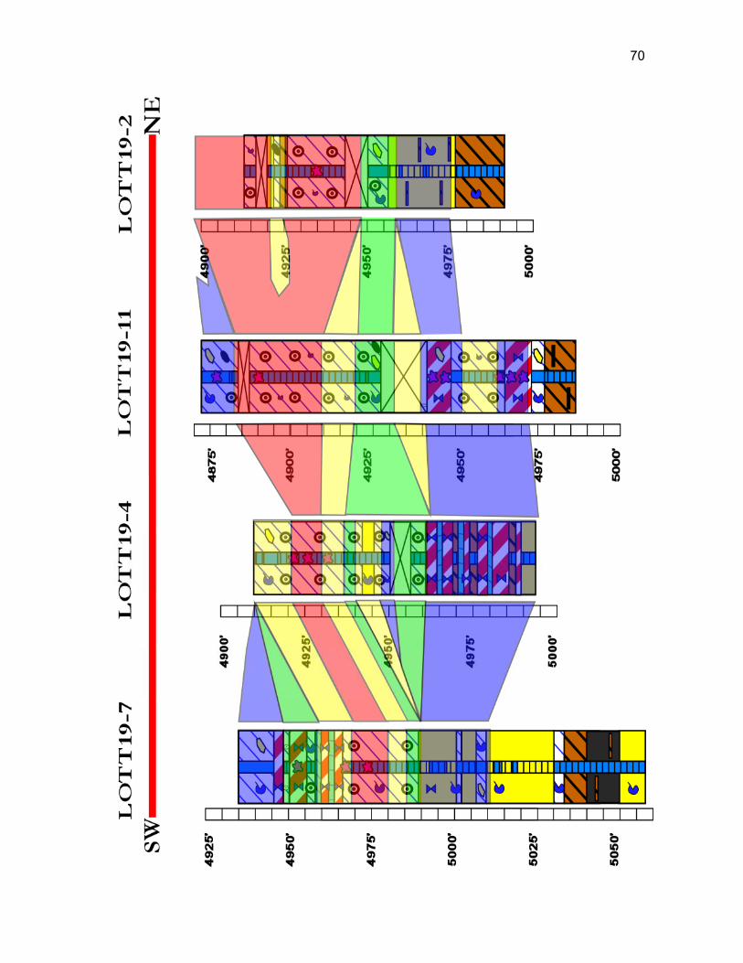
7070
71
Petrographic Image Analysis Predicting Capillary Pressure Behavior
Ten samples were chosen for Mercury injection capillary pressure (MICP)
experiments. The samples were chosen to represent good, intermediate, and poor
reservoir quality zones based on Hammel’s (1996) study. Slices were cut from the plugs
prior to injecting with mercury and thin sections were made from the slices. These thin
sections were examined by standard petrographic methods and by PIA to determine
whether thin section measurements on pores show any correlation to median pore throat
diameters (MTD) calculated from MICP data. If good correlation could be found, it
would indicate that image analysis data, in the form of median pore size (MPS) could
serve as proxies for MTD obtained by expensive and time-consuming MICP analyses.
Permeability depends on pore throat size and geometry. Figure 41 shows a close
correspondence between MTD and permeability. A plot of PIA porosity vs. MTD
(Figure 42) shows moderate correlation suggesting that MTD less than 2 microns may
exist in porosity values ranging from 4%-25%. But a positive relationship exists
between the porosity, abundance of pores, and the size of the throats that connect them.
Image analysis porosity vs. core K (Figure 43) shows good linearity and moderate
correlation, suggesting that porosity obtained from petrographic image analysis
techniques is a reasonable predictor of permeability. Table 3 summarizes data obtained
from the additional ten thin section samples.
Pore sizes and MTD were compared to determine if MTD correlate with pore
size obtained from image analysis methods. In siliciclastics this relationship is typical

72
Fig
ure
41.
Med
ian
thro
at d
iam
eter
vs.
cor
e pe
rmea
bili
ty.
Per
mea
bili
ty is
mos
t clo
sely
cor
rela
tive
to p
ore
thro
at a
pert
ure
size
, or
MT
D, a
nd th
is c
hart
sho
ws
exce
llen
t cor
rela
tion
wit
h a
coef
fici
ent o
f .9
081.
Med
ian
Thr
oat
Dia
met
er v
s. C
ore
K
Med
ian
Th
roat
Dia
met
er (
mic
ron
s)
Core K (md)
y =
28.
371x
– 3
3.52
3
R2 =
.908
1

73
Fig
ure
42.
Imag
e an
alys
is p
oros
ity
vs. m
edia
n th
roat
dia
met
er.
Thi
s gr
aph
indi
cate
s a
posi
tive
rel
atio
nshi
p
betw
een
poro
sity
per
cent
and
por
e th
roat
siz
e.
Imag
e A
nal
ysis
φ v
s. M
edia
n T
hroa
t D
iam
eter
Imag
e A
nal
ysis
φ (%
)
Median Throat Diameter(microns)
y =
.295
2x –
1.8
113
R2 =
.632
8

74
Fig
ure
43.
Imag
e an
alys
is p
oros
ity
vs. c
ore
perm
eabi
lity
. T
his
grap
h al
so s
how
s a
posi
tive
cor
rela
tion
betw
een
poro
sity
obt
aine
d fr
om P
IA a
nd c
ore
perm
eabi
lity
.
Imag
e A
nal
ysis
φ v
s. C
ore
K
Imag
e A
nal
ysis
φ (%
)
Core K (md)
y =
8.6
2x –
89.
6
R2 =
.610

75
Table 3. Summary of data from ten additional thin sections. Samples were collected at
two different times (Plug Set #1 and #2) and include various lithologies as well as a
spectrum of reservoir quality classes. Data includes well location, depth of sample, core
porosity, PIA porosity, core permeability, and MTD.
Slide # Well # Depth (ft) CoreN (%) PIAN (%) K (md) MPS (:m2) MTD (:m)
3 Lott 19 #11 4897.5 27.7 29.1 268 207 10.6
2 Lott 19 #2 4914.0 30.3 24.3 23.7 160 2.04
7 Lott 19 #4 4924.0 25.5 25.3 48 160 1.55
10 Lott 19 #11 4941.4 12 9.1 1.03 226 0.783
1 Lott 19 #5 4959.3 31.3 35.8 311 381 10.6
5 Lott 19 #7 4979.0 24.5 21.1 40 301 4.72
1 Lott 19 #7 4941.5 5.6 2.4 0.402 207 0.742
2 Lott 19 #4 4943.7 17.2 13.1 2.56 151 1.46
3 Lott 19 #7 4958.9 14 8.2 3.75 169 0.695
4 Lott 19 #8 4987.5 20.4 20.9 37.9 738 4.58
Plu
g S
et #
1P
lug
Set
#2
Slide # Well # Depth (ft) Core φ PIA φ K (md) MPS (µm2) MTD (µm2)

76
because pore size and pore throat size closely relate to sediment grain size. Carbonate
porosity is more complex and the relationship between pore size and pore throat size is
not as simple. For example, oomoldic pores may be very large and well developed, but
may be non-touching, in which case they exhibit anomalously small MTD
measurements. The prospect of predicting MTD from MPS measurements from PIA is
attractive. Figure 44 shows a plot of MTD vs. MPS. The data show that large pores
commonly have large pore throats associated with them. The dominant pore types
present at Happy field include oomolds (complete and incomplete), intergranular, and
vugs. Of these, vugs exhibit the largest average pore size of 800 square microns, yet
they do not have the largest pore throats because many vugs occur in muddy rocks that
lack intergranular connectivity. Figure 45 is a photomicrograph of large, non-touching
vugs in a skeletal wackestone packstone. This sample exhibits 21% porosity and 21 md
of permeability, a moderate quality reservoir rock.
Image analysis can serve as a reservoir characterization tool because pores may
be analyzed much more rapidly than with standard petrographic methods. Resulting data
on pore size, shape, frequency, origin, and overall abundance is easily obtained, enabling
a classification system to be formed based on the pore characteristics. Optimum poro-
perm pairs are predicted based on the identification of key pore attributes. These
attributes, in turn, are the basis for a classification scheme that estimates reservoir
quality.

77
Fig
ure
44.
Med
ian
pore
thro
at v
s. m
edia
n po
re s
ize.
A p
osit
ive
corr
elat
ion
is e
vide
nt a
nd th
e ou
tlie
r is
a sa
mpl
e w
ith
larg
e, is
olat
ed v
ugs.
M
edia
n T
hro
at D
iam
eter
vs.
Med
ian
Por
e S
ize
Med
ian
Th
roat
Dia
met
er (
mic
ron
s)
y =
15.
32x
+ 2
12.1
3
R2 =
.101
MedianPoreSize(micron2)

78
Figure 45. Photomicrograph of non-touching vugs. Sample is from Lott 19 #8 well,
4987.5’ and is seen on Figure 44 as the outlier data point. Scale bar is 100 microns.

79
CONCLUSIONS
1. Happy Spraberry field produces from heterogeneous, shallow-shelf carbonates where
lateral and vertical variations in porosity and permeability are common.
2. Porosity is predominantly a diagenetic overprint on depositional texture (grain-
moldic in oolitic grainstones).
3. Analyses of carbonate pores utilizing petrographic image analysis methods is a
relatively new procedure for gathering data on pore characteristics and is much faster
than standard petrographic methods.
4. Image analysis data were interpreted to identify 4 distinctive pore facies which, in
turn, are predictors of rock type, petrophysical properties, and production
characteristics.
5. Image analysis is a reasonable substitute for determining porosity values obtained by
alternate methods of core analyses, wireline log analyses, and standard petrographic
methods.

80
6. The highest quality reservoir rocks occur in oolitic grainstones and packstones and,
furthermore, the presence of moldic pores (oomoldic or skelmoldic) larger than
10,000 microns2 combined with large, solution enhanced intergranular pores provide
for optimum porosity and permeability.
7. Pore size obtained from petrographic image analysis is a useful predictor of median
pore throat aperture, which would otherwise only be available by performing
expensive Mercury injection capillary pressure tests.
8. Pitfalls of petrographic image analysis include choosing a magnification which gives
appropriate and accurate images of porosity, quality control on preparation of thin-
section samples, and consistent sampling of thin sections.
9. Petrographic image analysis has applicability in the geosciences (grain size,
paleontology, fractures…) here it was implemented as a reservoir characterization
tool within the carbonate interval at Happy Spraberry field.
81
REFERENCES CITED
Ahr, W.M. and B.S. Hammel, 1999, Identification and mapping of flow units in
carbonate reservoirs; An example from the Happy Spraberry (Permian) Field,
Garza County, Texas USA: Energy Exploration & Exploitation, v. 17, p.311-334.
Anselmetti, F. S., S. Luthi, and G.P. Eberli, 1998, Quantitative characterization of
carbonate pore systems by digital image analysis: AAPG Bulletin, v. 82, p. 1815-
1836.
Archie, G.E., 1952, Classification of carbonate reservoir rocks and petrophysical
considerations: AAPG Bulletin, v. 36, p. 278-298.
Asquith, G., 1997, Basic well log analysis for geologists, in G. Asquith and C. Gibson,
eds., AAPG Methods in Exploration 3, p. 66-90.
Atchley, S. C., M. G. Kozar, and L. A. Yose, 1999, A predictive model for reservoir
distribution in the Permian (Leonardian) Clear Fork and Glorieta formations,
Robertson Field area, West Texas: AAPG Bulletin, v. 83, p. 1031-1056.
Choquette, P.W., and L.C. Pray, 1970, Geologic nomenclature and classification of
porosity in sedimentary carbonates: AAPG Bulletin, v. 2, p. 207-250.
Dorobek, S. L., J.F. Read, and J.M. Niemann, 1987, Image analysis of
cathodoluminescent-zoned calcite cements: Journal of Sedimentary Petrology, v.
57, p. 766-770.
Dunham, R. J., 1962, Classification of carbonate rocks according to depositional
texture, in W. E. Ham, ed., Classification of carbonate rocks-a symposium:
AAPG Memoir 1, p. 108-121.

82
Ehrlich, R., S.J. Crabtree, K.O. Horkowitz, and J.P. Horkowitz, 1991a, Petrography and
reservoir petrophysics I: Objective classification of reservoir porosity: AAPG
Bulletin, v. 75, p. 1547-1562.
Ehrlich, R., E.L. Etris, D. Brumfield, L.P. Yuan, and S.J. Crabtree, 1991b, Petrography
and reservoir petrophysics III: Physical models for permeability and formation
factor: AAPG Bulletin, v. 75, p. 1579-1592.
Ehrlich, R., and J. P. Horkowitz, 1987, Estimation of petrophysics from thin section;
petrographic image analysis, in AAPG 1987 Southwest Section meeting;
abstracts: AAPG Bulletin, Tulsa, OK, American Association of Petroleum
Geologists, p. 238.
Ehrlich, R., S. K. Kennedy, S. J. Crabtree, and R. L. Cannon, 1984, Petrographic image
analysis; I, Analysis of reservoir pore complexes: Journal of Sedimentary
Petrology, v. 54, p. 1365-1378.
Hammel, B. S., 1996, High resolution reservoir characterization of the Permian (upper
Leonardian) Spraberry Formation, Happy Spraberry Field, Garza County, Texas:
Unpublished Master’s Thesis, Texas A&M University, 1996, 157 pp.
Handford, C. R., 1981, Sedimentology and genetic stratigraphy of Dean and Spraberry
formations (Permian), Midland Basin, Texas: AAPG Bulletin, v. 65, p. 1602-
1616.
Jeary, G. L., 1978, Leonardian strata in the northern Midland Basin of West Texas, in R.
L. Gilbertson, ed., Energy quest for the Southwest.: Publication - West Texas
Geological Society, Midland, TX, West Texas Geological Society, p. 30-47.

83
Lucia, F.J., 1983, Petrophysical parameters estimated from visual description of
carbonate rocks: a field classification of carbonate pore space: Journal of
Petroleum Technology, v. 35, p. 626-637.
Mazzullo, S. J., and W. E. Hipke, 1991, Evolution of a mixed carbonate-siliciclastic
platform; Lower Permian, northern Midland Basin, Texas, in AAPG Southwest
Section meeting; abstracts : AAPG Bulletin, Tulsa, OK, American Association of
Petroleum Geologists, p. 201.
Mazzullo, S. J. and A. M. Reid, 1989, Lower Permian platform and basin depositional
systems, northern Midland Basin, TX, in P.D. Crevello, J.L. Wilson, J.F. Sarg,
J.F. Read, eds., Controls on carbonate platform and basin development: SEPM
Special Publication No. 44, p. 305-320.
McCreesh, C. A., R. Ehrlich, and S.J. Crabtree, 1991, Petrography and reservoir
petrophysics II: Relating thin section porosity to capillary pressure, the
association between pore types and throat size: AAPG Bulletin, v. 75, p. 1563-
1578.
Montgomery, S. L., and W. H. Dixon, 1998, New depositional model improves outlook
for Clear Fork infill drilling: Oil and Gas Journal, v. 96, p. 94-98.
Mowers, T. T., and D. A. Budd, 1996, Quantification of porosity and permeability
reduction due to calcite cementation using computer-assisted petrographic image
analysis techniques: AAPG Bulletin, v. 80, p. 309-322.
Parham, K.D. and P.G. Sutterlin, 1993, Oolite shoals of the Mississippian St. Louis
formation, Gray County, Kansas: A guide for oil and gas exploration: in
Mississippian Oolites and Modern Analogs, Special Publication 35, p. 185-197.

84
Ross, C.A., 1986, Paleozoic evolution of southern margin of Permian basin: Geological
Society of America Bulletin, v. 97, p. 536-554.
Roy, E., 1998, High resolution mapping of flow units for enhanced recovery program
planning, Happy Spraberry Lime Field, Garza County, Texas: Unpublished
Master’s Thesis, Texas A&M University, 1998, 106 pp.
Sano, H., K. Horibo, and Y. Kumamoto, 1990, Tubiphytes-Archaeolithoporella-
Girvanella reefal facies in Permian buildup, Mino terrane, central Japan:
Sedimentary Geology, v. 68, p. 293-306.
Ward, R. F., C.G Kendall, and P.M Harris, 1986, Upper Permian (Guadalupian) facies
and their association with hydrocarbons-Permian basin, West Texas and New
Mexico: AAPG Bulletin, v. 70, p. 239-262.
Wardlaw, N. C., 1976, Pore geometry of carbonate rocks as revealed by pore casts and
capillary pressure: AAPG Bulletin, v. 60, p. 245-257.
Wardlaw, N.C., 1979, Pore systems in carbonate rocks and their influence on
hydrocarbon recovery efficiency: April 1979 short course on carbonate porosity,
Department of Geology, University of Calgary, Calgary, Canada, p. E1-E24.
Yang, K. M., and S.L. Dorobek, 1994, The Permian Basin of west Texas and New
Mexico: Tectonic history of a "composite" foreland basin and its effect on
stratigraphic development, in S.L. Dorobek and G. M. Ross, eds., Stratigraphic
evolution of foreland basins, SEPM Special Publication no. 52, p. 147-172.

85
APPENDIX A

86
Core DescriptionBennett PetroleumLott 19 #2Happy Spraberry FieldGarza County, TexasCore Interval 4914.0’-4944.0’
Depth (ft.) Thickness (ft.) Description
4914.0 2.0 Limestone. Light gray to dark brown, veryfine grained packstone, well sorted, mostlyooids/peloids and mollusk fragments, massive,grain moldic porosity, differential oil staining
4916.0 4.0 Core removed for special core analysis.
4920.0 2.0 Siltstone and shale. Dark gray, very fine grainedquartz silt and clay. Fossils rare. Parallel torippled laminations.
4922.0 3.0 Limestone. Brown to medium gray, moderatelysorted grainstone. Ooids, peloids, and lithoclasts.Brachiopods, crinoids, and mollusks, massive,differential oil staining.
4925.0 1.0 Siltstone. Light to medium gray, very finegrained quartz. Calcite cementation, rippled toplanar laminations, microfaults.
4926.0 9.0 Limestone. Medium gray to dark brown, wellsorted, fine grained grainstone. Rare fossils,massive, imbricated lithoclasts, grain moldic andvuggy porosity.
4935.0 1.0 Siltstone. Light to medium gray, fine grainedquartz. No fossils. Rippled laminations,microfaults.
4936.0 8.0 Limestone. Dark brown to medium gray, finegrained grainstone. Rare fossils, massive withisolated, planar ripples. Differential oil staining,vuggy and grain moldic porosity.

87
Core DescriptionBennett PetroleumLott 19 #2 (cont.)Happy Spraberry FieldGarza County, TexasCore Interval 4944.0’-4991.0’
Depth (ft.) Thickness (ft.) Description
4944.0 5.0 Core removed for special core analysis.
4949.0 1.0 Limestone. Light gray, moderately sortedpackstone. Composed of mostly ooids,lithoclasts, and skeletal fragments. Mollusks,crinoids, brachiopods, and ostracods common.
4950.0 5.0 Limestone. Medium gray to dark brown, wellsorted, fine grained grainstone. Massive,differential oil staining, grain moldic porosity.
4955.0 1.0 Sandstone. Light gray, moderately sorted veryfine grained sandstone with skeletal packstonestringers. Mollusk, crinoids common, planar,wavy laminations.
4956.0 8.0 Siltstone. Light gray to medium gray, well sortedquartz grains, fossils very rare. Discontinuouswavy laminations, microfaulted with contortedbedding.
4964.0 16.0 Siltstone. Medium gray to dark gray, moderatelysorted quartz grains. Fossils rare, Continuouswavy to planar laminations, microfaulted.
4980.0 11.0 Mudstone. Dark gray to black, well sorted clayparticles. Fossils rare, continuous wavylaminations.
4991.0 ----- END OF CORE.

88
Core DescriptionBennett PetroleumLott 19 #4Happy Spraberry FieldGarza County, TexasCore Interval 4910.0’-4948.0’
Depth (ft.) Thickness (ft.) Description
4910.0 2.0 Limestone. Medium gray to dark brown, finegrained, moderately sorted packstone. Rarefossils, lithoclasts, and ooids, massive. Grainmoldic porosity and differential oil staining.
4912.0 2.0 Limestone. Light gray, fine grained, well sortedgrainstone. Composed of ooids, skeletalfragments, massive, with grain moldic and vuggyporosity.
4914.0 3.0 Limestone. Medium gray, very fine grainedpackstone, composed of ooids and peloids.Massive with undifferentiated skeletal fragments.
4917.0 1.0 Siltstone. Tan to dark gray, very fine grainedquartz grains. Rare fossils, parallel to planarlaminations, microfaulted.
4918.0 24.0 Limestone. Medium gray to light gray, finegrained grainstone. Moderately sorted, rarefossils, composed primarily of ooids and peloids.Anhydrite pore-filling cement. Well-developedgrain moldic porosity.
4942.0 2.0 Limestone. Medium gray, fine grainedmoderately sorted silty packstone. Rare fossils,stylolites, microfaults, parallel, wavy, continuouslaminations.
4944.0 4.0 Light gray to dark brown, very fine grainedgrainstone, composed mostly of ooids andpeloids, burrowing.

89
Core DescriptionBennett PetroleumLott 19 #4 (cont.)Happy Spraberry FieldGarza County, TexasCore Interval 4948.0’- 4970.0’
Depth (ft.) Thickness (ft.) Description
4948.0 1.0 Limestone. Medium gray, moderately sorted finegrained packstone. Composed of skeletalfragments and ooids, wavy, discontinuouslaminations.
4949.0 2.0 Limestone. Medium gray to dark brown, finegrained grainstone, composed of ooids, peloidsand rare skeletal fragments. Massive, differentialoil staining, grain moldic and vuggy porosity.
4951.0 5.0 Core removed for special core analysis.
4956.0 5.0 Limestone. Medium gray to dark brown, finegrained grainstone, composed of ooids, peloidsand rare skeletal fragments. Massive, differentialoil staining, grain moldic and vuggy porosity.
4961.0 3.5 Limestone. Light gray to medium gray, coarsegrained, poorly sorted skeletal rudstone.Composed of oolitic grainstone lithoclasts andskeletal fragments, mostly of crinoid andbryozoan debris. Massive, brecciated texture.
4964.5 .5 Limestone. Medium gray to light tan, in situbiotic growth bindstone, mainly of bryozoans,ostracods, and crinoids. Growth fabric ofsediment trapping and binding organisms.
4965.0 5.0 Limestone. Medium gray to medium tan, coarsegrained skeletal, lithoclastic rudstone. Crinoids,mollusk, and oolitic grainstone lithoclasts.

90
Core DescriptionBennett PetroleumLott 19 #4 (cont.)Happy Spraberry FieldGarza County, TexasCore Interval 4970.0’-4981.0’
Depth (ft.) Thickness (ft.) Description
4970.0 1.0 Limestone. Light gray to light tan, in situ growthfabric. Fenestrate bryozoans, encrusting algae,Tubiphytes, and crinoids common.
4971.0 1.0 Limestone. Medium gray to dark tan , verycoarse grained, poorly sorted, lithoclastic,floatstone. Oolitic grainstone lithoclastsand skeletal fragments, mainly of crinoids andmollusks.
4972.0 5.0 Siltstone. Light tan to light gray, very finegrained quartz grains with calcite cement.Parallel to wavy laminations, microfaulted.
4977.0 2.0 Limestone. Light gray, very coarse grainedlithoclastic rudstone. Lithoclasts are composedprimarily of oolitic grainstone and skeletalfragments.
4979.0 1.5 Limestone. Medium gray to dark gray, poorlysorted lime floatstone. Shaly matrix with isolatedskeletal and lithoclasts fragments. Crinoid andbryozoan fragments common, with rare ooids andpeloids.
4980.5 .5 Limestone. Medium gray to medium tan, in situbindstone biotic growth. Bryozoans,brachiopods, and crinoids common. Anhydritepore-filling cement.

91
Core DescriptionBennett PetroleumLott 19 #4 (cont.)Happy Spraberry FieldGarza County, TexasCore Interval 4981.0’-4994.0’
Depth (ft.) Thickness (ft.) Description
4981.0 4.0 Limestone. Medium gray to light tan, poorlysorted, floatstone. Silty matrix with light tanskeletal rudstone breccia. Composed of mostlycrinoid, bryozoan, and mollusk fragments.
4985.0 1.0 Limestone. Dark gray to light gray, coarsegrained rudstone. Fossils common withlithoclasts. Massive structure with brecciatedtexture.
4986.0 1.0 Limestone, dark gray to black, poorly sorted limefloatstone. Silty shale matrix with rudstone andbindstone lithoclasts, fossil fragments of crinoidsand bryozoans common.
4987.0 2.0 Limestone. Dark gray to black, very fine grainedmudstone. No fossils, wavy continuous todiscontinuous laminations, microfaults, contortedbedding.
4989.0 2.0 Limestone. Dark gray, poorly sorted limefloatstone. Shaly matrix with rudstone andbindstone lithoclasts, fossil fragments of crinoids,bryozoans, and Tubiphytes.
4991.0 3.0 Siltstone. Dark gray to medium gray, very finegrained quartz. Isolated skeletal fragments,including ostracods, brachiopods, and crinoids.Continuous, wavy laminations.
4994.0 ----- END OF CORE.
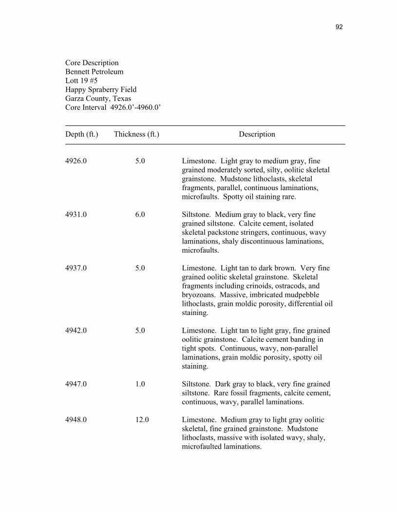
92
Core DescriptionBennett PetroleumLott 19 #5Happy Spraberry FieldGarza County, TexasCore Interval 4926.0’-4960.0’
Depth (ft.) Thickness (ft.) Description
4926.0 5.0 Limestone. Light gray to medium gray, finegrained moderately sorted, silty, oolitic skeletalgrainstone. Mudstone lithoclasts, skeletalfragments, parallel, continuous laminations,microfaults. Spotty oil staining rare.
4931.0 6.0 Siltstone. Medium gray to black, very finegrained siltstone. Calcite cement, isolatedskeletal packstone stringers, continuous, wavylaminations, shaly discontinuous laminations,microfaults.
4937.0 5.0 Limestone. Light tan to dark brown. Very finegrained oolitic skeletal grainstone. Skeletalfragments including crinoids, ostracods, andbryozoans. Massive, imbricated mudpebblelithoclasts, grain moldic porosity, differential oilstaining.
4942.0 5.0 Limestone. Light tan to light gray, fine grainedoolitic grainstone. Calcite cement banding intight spots. Continuous, wavy, non-parallellaminations, grain moldic porosity, spotty oilstaining.
4947.0 1.0 Siltstone. Dark gray to black, very fine grainedsiltstone. Rare fossil fragments, calcite cement,continuous, wavy, parallel laminations.
4948.0 12.0 Limestone. Medium gray to light gray ooliticskeletal, fine grained grainstone. Mudstonelithoclasts, massive with isolated wavy, shaly,microfaulted laminations.

93
Core DescriptionBennett PetroleumLott 19 #5 (cont.)Happy Spraberry FieldGarza County, TexasCore Interval 4960.0’-5025.0’
Depth (ft.) Thickness (ft.) Description
4960.0 5.0 Core removed for special core analysis.
4965.0 2.0 Siltstone. Dark gray to medium gray, very finegrained siltstone with interbedded skeletalpackstone stringers. Wavy, continuous, parallellaminations with microfaults.
4967.0 5.0 Limestone. Light tan to medium brown, finegrained, well sorted, oolitic and skeletalgrainstone. Common ostracods, crinoids, andmollusks. Spotty oil staining with welldeveloped grain moldic porosity.
4972.0 1.0 Limestone. Medium tan, poorly sorted, ooliticgrainstone. Lithoclast present include reefyfragments as well as whole fossils. Grain moldicporosity.
4973.0 4.0 Siltstone. Light gray to medium gray, very finegrained quartz. Fossil fragments, calcite cementcommon, discontinuous, non-parallellaminations.
4977.0 7.0 Mudstone. Dark gray to black mudstone. Wavy,discontinuous laminations, microfaults, andcontorted bedding.
4984.0 3.0 Siltstone. Medium gray very fine grained quartz.Fossil fragments rare, discontinuous, non-parallellaminations, microfaults.
4987.0 38.0 Lost core.

94
Core DescriptionBennett PetroleumLott 19 #5 (cont.)Happy Spraberry FieldGarza County, TexasCore Interval 5025.0’
Depth (ft.) Thickness (ft.) Description
5025.0 ----- END OF CORE.

95
Core DescriptionBennett PetroleumLott 19 #7Happy Spraberry FieldGarza County, TexasCore Interval 4936.0’-4969.0’
Depth (ft.) Thickness (ft.) Description
4936.0 7.0 Siltstone. Light gray to light tan, very finegrained siltstone with interbedded skeletalpackstone stringers. Skeletal fragments consistof mollusks, crinoids, and bryozoans.Continuous, parallel laminations withmicrofaults.
4943.0 3.0 Limestone. Medium gray, moderately sorted,silty skeletal packstone. Rare lithoclasts, crinoidfragments. Continuous, parallel, wavylaminations with microfaults.
4946.0 1.0 Siltstone. Medium gray to dark gray, very finegrained siltstone. Fossils rare, wavy, continuous,parallel laminations with microfaults.
4947.0 3.0 Limestone. Light gray to light tan, fine grained,well sorted, grainstone. Composed primarily ofooids and peloids. Skeletal fragments common,rare anhydrite cement, massive. Differential oilstaining with grain moldic porosity.
4950.0 19.0 Limestone. Light gray to dark tan, poorly sortedskeletal rudstone/packstone. Anhydrite cementcommon, fossils include ostracods, bryozoans,mollusks, and crinoids, massive, non-bedded.Vuggy and grain moldic porosity, differential oilstaining.

96
Core DescriptionBennett PetroleumLott 19 #7 (cont.)Happy Spraberry FieldGarza County, TexasCore Interval 4969.0’-5010.0’
Depth (ft.) Thickness (ft.) Description
4969.0 1.0 Limstone. Light gray to medium gray, poorlysorted, silty, lime wackestone. Wavy,discontinuous, non-parallel laminations,stylolites, and lithoclasts.
4970.0 18.0 Limestone. Medium gray to dark tan, poorlysorted, skeletal rudstone/packstone. Fossilsinclude mollusks, bryozoans and crinoids.Massive, non-bedded, brecciated texture. Vuggyand grain-moldic porosity, differential oilstaining.
4988.0 8.0 Siltstone. Light gray to light tan, well sortedvery fine grained quartz grains. Rare, isolatedskeletal fragments. Discontinuous, non-parallel,wavy laminations with microfaults.
4996.0 2.0 Limestone. Light gray, poorly sorted, siltyskeletal lithoclastic rudstone. Brecciated texture,massive.
4998.0 6.0 Siltstone. Dark gray to medium gray, wellsorted, fine grained quartz grains.Discontinuous, wavy, non-parallel laminationswith microfaults.
5004.0 6.0 Siltstone. Moderately sorted, fine grained quartzgrains. Minor lithoclasts with skeletal fragmentscomposed primarily of crinoids and mollusks.Anhydrite cement with no visible porosity.

97
Core DescriptionBennett PetroleumLott 19 #7 (cont.)Happy Spraberry FieldGarza County, TexasCore Interval 5010.0’-5057.0’
Depth (ft.) Thickness (ft.) Description
5010.0 32.0 Siltstone. Light gray to medium gray, wellsorted, very fine grained quartz. Continuous,wavy, parallel laminations. No fossils.
5042.0 9.0 Mudstone. Dark gray to black, moderatelysorted, very fine grained silty mudstone. Isolatedcontinuous, parallel laminations with microfaults.
5051.0 6.0 Siltstone. Medium gray, moderately sorted, finegrained quartz. Fossil fragments of crinoids andbryozoans common. Continuous, parallel, wavylaminations.
5057.0 ----- END OF CORE.

98
Core DescriptionBennett PetroleumLott 19 #11Happy Spraberry FieldGarza County, TexasCore Interval 4873.0’-4927.0’
Depth (ft.) Thickness (ft.) Description
4873.0 8.0 Limestone. Medium tan to light gray,moderately sorted, fine grained ooliticgrainstone. Anhydrite replacement cement, fossilsrare. Isolated continuous, wavy, parallellaminations, with minor microfaults. Grainmoldic porosity and differential oil staining.
4881.0 2.0 Limestone. Light gray to light tan, poorlysorted, oolitic grainstone with mud pebblelithoclasts. Anhydrite cement, grain moldicporosity.
4883.0 1.0 Limestone. Light tan, well sorted, fine grainedoolitic grainstone. Fossils rare, grain moldicporosity, differential oil staining.
4884.0 2.0 Lost core.
4886.0 38.0 Limestone. Light gray to medium tan, wellsorted, fine grained oolitic skeletal grainstone.Anhydrite replacement cement, abundant fossilfragments, including mollusks, ostracods, andcrinoids. Massive, non-bedded, grain moldicporosity of ooids and skeletal fragments,differential oil staining.
4924.0 3.0 Limestone. Light gray to medium gray,moderately sorted, fine grained, silty, ooliticskeletal packstone. Anhydrite cement, withisolated continuous, wavy, parallel laminations.Skeletal grainstone stringers with grain moldicporosity.

99
Core DescriptionBennett PetroleumLott 19 #11 (cont.)Happy Spraberry FieldGarza County, TexasCore Interval 4927.0’-4986.0’
Depth (ft.) Thickness (ft.) Description
4927.0 14.0 Lost core.
4941.0 11.0 Limestone. Light gray to medium gray, poorlysorted, skeletal rudstone. Pervasive anhydritecement, abundant skeletal fragments, includingbryozoans, mollusks, crinoids, and ostracods.Massive with stylolites and differential oilstaining.
4952.0 5.0 Limestone. Light gray to light tan, well sorted,fine grained skeletal packstone grainstone.Massive, fossils include mollusks, bryozoans,and crinoids. Vuggy porosity and differential oilstaining.
4957.0 19.0 Limestone. Light gray to medium tan, poorlysorted, skeletal rudstone. Pervasive anhydritecement, fossils include mollusks and bryozoanswith some intervals as in situ bindstones. Vuggyporosity with differential oil staining.
4976.0 1.0 Siltstone. Medium gray, moderately sorted, veryfine grained quartz with isolated fossil fragments.Isolated packstone stringer, contorted beddingand soft sediment deformation.
4977.0 9.0 Siltstone. Medium gray to dark gray, very finegrained quartz grains with interbedded mudstone.No fossils, wavy, continuous, parallellaminations with microfaults.
4986.0 ----- END OF CORE.

100
APPENDIX B

101
Lott 19 #4 Petrographic Data

102
Lott 19 #7 Petrographic Data

1
VITA
NAME: John Morgan Layman II
PERMANENT John M. LaymanADDRESS: 2732 Ferguson Drive
Harrisonburg, VA 22801
EDUCATION: Texas A&M UniversityCollege Station, TXM.S. Geology, 2002
James Madison UniversityHarrisonburg, VAB.S. Geology, 1995
PROFESSIONAL TotalFinaElf Exploration and Production, Inc. `EXPERIENCE: Onshore Production and Development, 2001
PROFESSIONAL American Association of Petroleum GeologistsMEMBERSHIP: Geological Society of America
Houston Geological SocietySociety for Sedimentary Geology (SEPM)
PUBLICATIONS:
LAYMAN II, JOHN M., and Wayne M. Ahr, Texas A&M University, Department of
Geology & Geophysics, College Station, TX 77845; Pore Measurements by
Petrographic Image Analysis: Implications for Rapid Identification and Ranking of
Reservoir Flow Units, Happy Spraberry Field, Garza County, Texas: AAPG Bulletin, v.
85 (2001), no. 13 Supplement.
LAYMAN II, JOHN M., and Wayne M. Ahr, Texas A&M University, Department of
Geology & Geophysics, College Station, TX 77845; Pore Measurements by
Petrographic Image Analysis: Implications for Rapid Identification and Ranking of
Reservoir Flow Units, Happy Spraberry Field, Garza County, Texas: AAPG Bulletin, v.
84, no. 11 (November 2000), p. 1867.
LAYMAN II, JOHN M., Texas A&M University, Department of Geology &
Geophysics, College Station, TX 77845; Pore Measurements by Petrographic Image
Analysis: Implications for Rapid Identification and Ranking of Reservoir Flow Units,
Happy Spraberry Field, Garza County, Texas: GSA Abstracts with Programs, 2000, v.
32, no. 7, p. 178.
103