pore-fluid pressure and heat flow surveys along the

R/V Kronprins Haakon

15-31 October 2020

Tromsø-Longyearbyen

CAGE20-6 Cruise Report

Pore-fluid pressure and heat flow surveys along the Vestnesa Ridge, west-Svalbard

continental margin

Chief scientist: Andreia Plaza-Faverola

Captain: Johnny Peder Hansen

1. Introduction

CAGE20-6 cruise on board R/V Kronprins Haakon to the west Svalbard margin is the third research expedition

of the SEAMSTRESS project – Tectonic stress effects on Arctic methane seepage (2019-2023). The project and

therefor the cruise is primarily funded by the Tromsø Research Foundation (TFS) and the Research Council of

Norway (RCN project number 287865) through their starting grant schemes. The project and cruises are also

supported by the Department of Geosciences and the Center for Arctic gas hydrates, environment and

climate at UiT – The Arctic University of Norway.

SEAMSTRESS is investigating how the stress generated by regional processes in Arctic margins (e.g., mid-

ocean ridge spreading, glacial advance and retreat, tides, gravitational forcing) affect pore fluid pressure and

seepage.

Cruise CAGE20-6 focusses on the Vestnesa Ridge fluid flow system (figure 1) and the main cruise objective is

to search for spatial pressure and temperature variations along the ridge. We use the Ifremer Piezometer for

in-situ pore fluid pressure measurements and the newly acquired UiT heat flow probe for

temperature/conductivity measurements and heat flow calculations.

The in-situ pressure survey along the Vestnesa Ridge started in 2019 during CAGE19-3 cruise [Knies et al.,

2019; Sultan et al., 2020] the first SEAMSTRESS expedition) and continues this year. This year we collected

pressure data from 4 piezometer stations and heat flow data from 27 stations. In addition chirp and sonar

data as well as gravity cores are available from each super station.

The regional heat flow survey is intended as a large project to complete the survey by Crane et a., started in

the 90s [Crane et al., 1991]. The obtained heat flow data will allow further constraining the dynamics of the

bottom simulating reflection (BSR) along the Vestnesa Ridge [e.g., Plaza‐Faverola et al., 2017] and further

constraining spreading rates of the Molloy and Knipovich mid- ocean ridges [e.g., Johnson et al., 2015]

Figure 1 Study area and locations of the data acquired during CAGE20‐6

2. Scientific crew

Andreia Plaza-Faverola, Researcher CAGE-UiT (Cruise leader)

Sunil Vadakkepuliyambatta, Researcher CAGE-UiT (Leader acoustics, data managing and responsible Heat

Flow)

Nabil Sultan, Research Ifremer (responsible Piezometer data)

Stephan Ker, Research Ifremer (responsible Ocean Bottom Seismometer data)

Mickael Roudaut, technician Ifremer (Piezometer and OBSs)

Anthony Ferrant, technician Ifremer (Piezometer and OBSs)

Truls Holm, engineer UiT (Heat flow and gravity coring)

Jan Vidar Nordstrand, IMR (Acoustic instruments)

Roy Robertsen, IMR (Acoustic instruments)

Hanne Børsheim, IMR (Acoustic instruments)

Sunny Singhroha, Researcher CAGE-UiT (shifts cross-communication, data integration)

Frances Cooke, PhD student UiT (chirp data processing, gravity coring)

Przemyslaw Domel, PhD student UiT (sonar data processing, gravity coring)

Rémi Vachon, Post doc UiT (main gravity coring)

Hariharan Ramachandran, Post doc UiT (sonar data processing, gravity coring)

3. Equipment

3.1 CTD

The CTD measures acoustic velocity, conductivity, temperature and other relevant oceanographic

information based on sensors used in the device. Water column acoustic velocities from CTD measurements

are used in the EK80 single-beam echosounder and EM302 multibeam echosounder for bathymetric

mapping. The CTD instrument used on the cruise is the SBE11 plus from Seabird Scientific. The CTD system

consists of the Seabird SBE 11 plus deck unit connected to bottle SBE32 carousel for water sampling. The CTD

is equipped with the following sensors: 2 x SBE3 Temperature sensors (s/n: 4535 and 4306), 2 x SBE4

Conductivity sensors (s/n: 4386 and 2799), 2 x SBE43 oxygen sensors (s/n: 3947 and 3949), 1x PSA916

Altimeter (s/n: 73084), 1x pressure sensor (s/n: 141612), 1 x Wet Labs C-Star beam transmissometer (s/n:

CST-2003 DR(420-461)), 1x Wet Labs ECO-AFL/FL Fluorometer (s/n: FLRTD-1547, FLRCDRTD-1930), and 1 x

Biospherical PAR sensor (s/n: 70736) with Surface PAR (s/n: 20568) added. 2 pumps (s/n: 9378 and 9379) are

used to make water run through these sensors. The CTD measures parameters at 44Hz and uses Seasave win

7.26.7.107 for data logging. SBE Data processing v. 7.26.7 is used for post-data processing. Figure 2 shows

profile from different measurements at CTD location (Figure 2).

Figure 2: Temperature, density, sound velocity and salinity measured at CTD station 1.

3.2 Kongsberg SBP300 Sub-bottom profiler

The data were recorded using the hull-mounted Kongsberg SBP300 MK2 and software system version 1.6.6.

The maximum depth of penetration is 100ms TWT (approximately 30 metres) over contourite drifts (Figure

3). The chirp pulse form is ‘linear chirp up’ with 30ms sweep length and frequencies between 2.5 and 7 kHz.

The transmit power starts with a soft setting -30dB and gradually increases (over 2.5 minutes) to -5dB. The

ping rate and bottom tracking is externally controlled by the EM302 multibeam system, and varies with

depth. Typically at water depth of 1000m a ping interval of 4 seconds is suitable. Sample interval is 48 kHz

with an acquisition time window of 500 ms. The vessel velocity is 4-5 knots while surveying and during

transits 8 knots. The average trace (along track) interval for a 5 knot survey (ship speed we used) is

approximately 10m.

The sweep function from the signal is removed using a matched filter based on autocorrelation of the Klauder

wavelet. Gain correction is applied, which corrects for spherical loss of the acoustic pressure wave in the

water column. Time variable gain is also applied prior to the logging of the processed sequence. The vertical

resolution is 0.15m, using a sound velocity of 1500 m/s, typical of sea water and shallow sediments. The

acquisition processing applies the envelope function to the data (instantaneous amplitude) which improves

the signal-to-noise ratio. The signal phase of the data is removed and displays positive amplitudes only. This

is the standard for interpretation of chirp data. The segy data, output from the Kongsberg acquisition system

is in data format 4 byte IEEE float. The same file format is used while processing in Seismic Unix (SU). Files

with the suffix ‘_UTMXXN’ are files output from SU. The XY coordinates are stored in byte positions 73 and

77 and copied to 81 and 85. The data are projected to Universal Transverse Mercator zones (UTM), for which,

31N is the zone used for the data acquired in this survey. The UTM zone number can also be found in byte

position 21 (CDP). The data are logged with varying delay recording time (delrt) to reduce file size in

acquisition. When required, the data are shifted back to a constant delay recording time in SU. The range of

the minimum and maximum time values are expanded, when final processing reveals a partial display of data,

with data muted outside of the 500ms acquisition time window.

Interpretation

Horizons interpreted in Chirp data from survey CAGE19_3 were used to extend age estimates (Figure 3)

acquired using data from the MARUM-MeBo-70 sediment drill rig and gravity core data [Himmler et al., 2019;

Schneider et al., 2018] and Dessandier et al., in review.

Figure 3: Example of sub‐bottom profile data

3.3 EM302 Multibeam sonar data

We used EM302 multibeam system by Kongsberg to study seafloor and water column in the vicinity of

Vestnesa Ridge. The system works by sending hundreds of electromagnetic pulses in horizontal swaths that

travel through the seafloor, get reflected, and are subsequently received back. The frequency of

electromagnetic beams sent is 30 kHz. Resolution of the system depends on the number of the beams shot

and the area they ultimately cover at the seafloor (with increasing depth resolution decreases). For our

survey, we used 432 beams, covering in total 90 degrees in angular resolution (45 degree each side from

vertical position). So the horizontal resolution can be given as:

resolution=depth x tan(beam_range_per_side) / no_of_beams_per_side

We were conducting surveys in areas with depths ranging from 1200 m to about 2500 m. For 1200 m (depth

of the crest at the east of Vestnesa Ridge), the horizontal resolution of the system with 216 beams per side

covering 45 degrees equaled 5,55 m. Resolution in the direction of the ship traversal depends on the speed

of the ship and the depth of the water (greater depth requires more time between each pinging). The speed

of pinging is controlled by the multibeam system itself and for the ship speed of 5 knots we have around 4

meter separation between each swath at the seabottom.

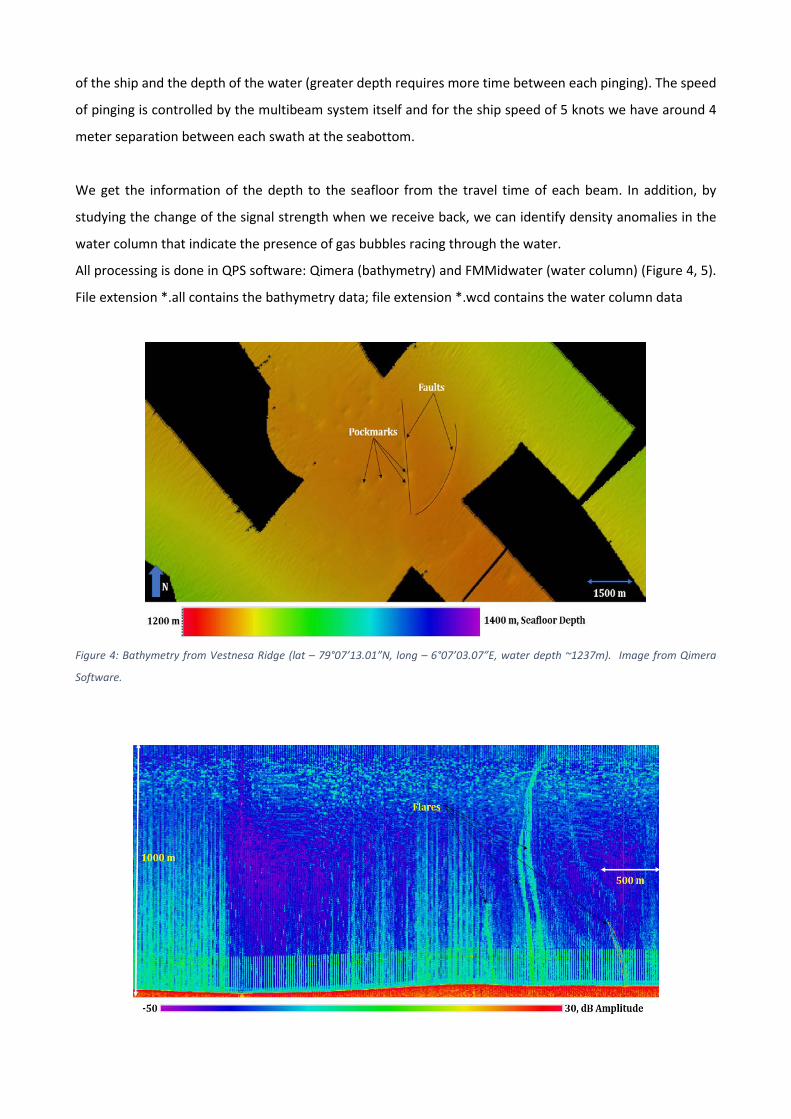
We get the information of the depth to the seafloor from the travel time of each beam. In addition, by

studying the change of the signal strength when we receive back, we can identify density anomalies in the

water column that indicate the presence of gas bubbles racing through the water.

All processing is done in QPS software: Qimera (bathymetry) and FMMidwater (water column) (Figure 4, 5).

File extension *.all contains the bathymetry data; file extension *.wcd contains the water column data

Figure 4: Bathymetry from Vestnesa Ridge (lat – 79°07’13.01”N, long – 6°07’03.07”E, water depth ~1237m). Image from Qimera

Software.

Figure 5: Stacked water column data from Vestnesa Ridge (lat – 79°00’10.77”N, long – 6°55’28.25”E, water depth ~1237m). Image

from FMMidwater Software.

3.4 Gravity corer

UiT’s gravity corer (GC) has a total weight of ~1000 kg. It consists of a 6 m long steel barrel with an inner

diameter of 11 cm, a steel-mantled led weight at the top, and a core head with a core catcher at the bottom.

For each deployment, a 5.95 m black plastic liner (pipe) with an outer diameter of 11 cm and inner diameter

of 10 cm is inserted into the steel barrel. The gravity core is lifted horizontally by two slings attached to a

crane while hooked up to the traction winch rope. The gravity core is lowered through the water column at

1m/s and further through the sediments by its own weight.

After retrieval, the plastic liners were manually cut into sections of up to 100 cm length, while taking care of

the plastic sawdust (a significant amount of plastic is released form the cutting procedure; we collected as

much as possible from the deck to avoid it going to the sea). The section ends were secured with plastic caps

and the sections were labelled.

3.5 Heat flow Probe

To measure the in situ subsurface thermal regime and thermal conductivities of sediments, the FIELAX deep-

sea heat flow probe is employed (Figure 6). The probe consists of a series of 22 thermistors and heating

elements placed within a sensor string ~6.05 m long. The thermistors are places 0.26 cm apart and is designed

for a temperature range of -2 to 60 0C with a resolution of 1 mK and accuracy of 2 mK after calibration. The

sensor string is attached to a strength member, which bears the load while penetrating the sediments. The

head section of the heat flow probe consists of data acquisition and power supply units. The whole probe

weighs ~1100 kg and is rated for operation up to 6000 meters water depth.

Figure 6: UiT’s heat flow probe being deployed from the starboard side of RV Kronprins Haakon (left).Data acquisition unit housed in

the head‐section of the heat‐flow probe(right). Red LED indicates that the acquisition unit is switched on. A blinking LED suggests that

the system is recording data.

The data acquisition unit records the data from the sensor string and sends the heat pulse energy to the

heating wires on the sensor string (Figure 6). It hosts a high-precision temperature sensor PT100, can

measure tilt in two axes as well as the vertical acceleration. The pressure data from PT100, tilt, and vertical

acceleration are used to configure the triggering of heat pulse and period of recording, whereas the

temperature data from PT100 is used to calibrate the thermistors on the sensor string. In situ thermal

gradients are calculated using the temperatures measured by the thermistors, whereas in situ thermal

conductivity is estimated using the heat pulse method [Lister et al., 1990], where the sensor string is heated

up for 20 s and thermal conductivity is derived from the following temperature decay. The post-processing

and quality control of the data was performed using Fellow software from Fielax, which estimates thermal

gradients, thermal conductivity, and heat flow for each penetration.

The thermistors must be calibrated with temperature measurements from PT-100 sensor before each

survey for accurate measurements. This was performed during the first deployment of the heat flow probe,

where the tool was lowered to 1271 m water depth, where the temperature in the water column is

constant over 10 m (data from CTD 199) and kept for 10 minutes. Calibration data is shown in the table

below.

Sensor Temp.(degC) DeltaT PT100 -0.7721

S1 -0.8009 -0.0288 S2 -0.7640 0.0369 S3 -0.8202 -0.0562 S4 -0.8315 -0.0113 S5 -0.7788 0.0527 S6 -0.7994 -0.0206 S7 -0.7639 0.0355 S8 -0.7916 -0.0277 S9 -0.8437 -0.0521

S10 -0.8235 0.0202 S11 -0.7705 0.0530 S12 -0.7738 -0.0033 S13 -0.8354 -0.0616 S14 -0.7702 0.0652 S15 -0.7978 -0.0276 S16 -0.8221 -0.0243 S17 -0.7657 0.0564 S18 -0.7958 -0.0301 S19 -0.7812 0.0146 S20 -0.7875 -0.0063 S21 -0.7664 0.0211 S22 -0.7620 0.0044

Table 1 Temperatures measured at 22 thermistors on the sensor string and its variance with precision PT100 sensor on the data acquisition unit.

During CAGE20-6, in-situ temperatures were measured at 27 stations involving 83 successful penetrations

(Figure 7). The main aims for the heat flow survey were to obtain high-resolution background heat flow

measurements on the Vestnesa Ridge, and to identify fine-scale variations in thermal properties of

sediments in the elongated depression North of Knipovich Ridge.

Figure 7 Overview of the heatflow stations during CAGE20‐6. Stations 20‐24 are at and around the elongated depression, whereas other stations were used to constrain the background heatflow over Vestnesa Ridge.

Two different styles of data acquisition were employed for achieving these goals. Over the Vestnesa Ridge,

the heat flow probe was deployed over the starboard side of the vessel and allowed to penetrate the

sediments at a winch speed of ~1.0 m/s. The tool was then kept stable for 15-20 minutes (to allow for

temperature decay after frictional heating during penetration) before a heat pulse was released. The tool is

kept on the seafloor for another 15-20 minutes to allow for the heat pulse to decay. The probe was then

pulled out at a winch speed of ~0.2m/s to ~50 m above the seafloor and the ship moved to a nearby

position ~50 m away. The probe was then allowed to penetrate again and record for 10-15 minutes. This

process is repeated one more time before taking the tool up onboard. No heat pulse is triggered during the

second and third penetrations. The last two penetrations were used to validate the thermal gradient

measured during the first penetration. At the elongated depression, north of Knipovich Ridge, a ‘pogo-style’

heat flow measurement was conducted (Figure 8). Here, the probe was kept stable within the sediments

for 20 minutes before the heat pulse was triggered. The probe is then kept stable for another 20 minutes to

allow for heat pulse decay. Then, the probe was pulled to and moved to the next station 500 m away and

lifted above 50 m to release the next heat pulse before penetration. The procedure is then repeated (Figure

8).

Figure 8 Overview of the “Pogo‐Style” measurements with the heat flow probe.

During the measurements at both areas, the heat pulse was set to release while the probe was stable for

15-20 minutes, and the tilt was within 100 with fluctuations within 0.50, and acceleration fluctuations within

0.01 (A2). Recording of the data started during deployment and stopped after bringing the probe back

onboard (A1). The distance limit for activating a second heat pulse (A3), was set at 100 dbar during the

Vestnesa measurements and at 50 dbar for the measurements at elongated depression (Figure 8).

3.6 Ifremer Piezometer

The Ifremer piezometer is a free-fall device with a sediment-piercing lance attached to a recoverable

instrument part (Error! Reference source not found.). It is ballasted with lead weights (up to 1000 kg) to

penetrate a range of sediment types in water depths of up to 6000 m. The length of the lance used depends

on the stiffness of the sediment with a maximum length of 12 meters. Pore pressures are measured relative

to hydrostatic pressure at different ports on the 60 mm diameter lance using specially adapted differential

pressure transducers connected to the pressure ports and the open seawater. The piezometer pore pressure

sensors have an accuracy of ± 0.5 kPa. The piezometer lance is also equipped with temperature sensors

located at the same level as the pore pressure sensors. Temperature sensors have an accuracy of 0.05 °C.

Figure 9 Schematic of the Ifremer Piezometer.

During this cruise two piezometers of 9.11 m length equipped with 9 temperature and 8 pressure sensors

(Error! Reference source not found.) were used (during CAGE19-3 cruise only one piezometer was taken

onboard). The first temperature sensor is in the water-column (around 0.5 m above the seabed) while the

other 8 sensor depths are between 0.79 and 8.64 m (Error! Reference source not found.).

Section length (m) Sensor names Sensor depth (mbsf)

T0 In the water column (around 0.5

m above the seabed)

0.75 T1, P1 0.79

0.75 T2, P2 1.59

1.50 T3, P3 3.14

1.50 T4, P4 4.69

1.50 T5, P5 6.24

0.75 T6, P6 7.04

0.75 T7, P7 7.84

0.75 T8, P8 8.64

Total lance length (cm) 9.11

Table 2 Piezometer characteristics and position of sensors.

We carried-out four deployments in the study area (Vestnesa ridge – offshore Svalbard) with recording

periods between 2.75 and 3.5 days (Error! Reference source not found.). The aim is to determine the

hydraulic properties of the near-surface sediment and to characterize the in-situ hydraulic and thermal

regimes.

Simplified

names

Sites # of sensors Coordinates Water depth

(m)

Recording period

(Time UTC)

STR2-PZ1 CAGE20-6-KH-12-

PZM-01

8 P and 9 T 79° 7.242 N

6° 08.088 E

1234 20/10/2020 18:22

23/10/2020 19:52


PZM-01

8 P and 9 T 79° 0.285 N

6° 56.123 E

1207 21/10/2020 19:45

24/10/2020 19:09


PZM-02

8 P and 9 T 79° 6.747 N

6° 12.104 E

1228 23/10/2020 23:00

27/10/2020 10:17


PZM-02

8 P and 9 T 78° 52.891 N

7° 28.596 E

1127 25/10/2020 02:06

27/10/2020 18:46

Table 3 Piezometer names and recording periods; STR2 is short for SEAMSTRESS2.

3.7 Ifremer Ocean Bottom Seismometers

Ifremer short-period 4-component OBSs are MicrOBS from SERCEL (Figure 10): one hydrophone, a vertical

geophone and two horizontal geophones. The sampling frequency is 1000 Hz (Table 4), the natural frequency

of geophones is 4.5 Hz and the cut-off frequency of the hydrophone is 2Hz. In addition, a large band

autonomous hydrophone (200 kHz) was installed on the piezometer PZ2 (79° 0.285; 6°56.123, 2020/10/21

at 19H45). The autonomy of this instrument was 5 hours. OBS locations, drift times, and technical details are

summarized in tables 4-8.

MicrOBS Setup Parameters

Sampling Frequency 1000 Hz

Hydro/geo Gain 20 dB / 26 dB (1x/2x)

Filter option FIR2

Drift values (ms): -9;-78;u;-13;5

Table 4 OBS setup parameters

Hyrdophone Setup Parameters

Sampling Frequency 512kHz

Time shift (ms): +50

Table 5 Hydrophone setup parameters

Mircrobs Depth Latitude Longitude

OBS1 1196 78°59.86519 6°57.39578

OBS2 1196 79°00.02276 6°56.49431

OBS3 1137 79°00.12687 6°55.87014

OBS4 1208 79°00.37879 5°55.73538

OBS5 1201 79°00.20266 6°54.49714

Table 6 OBSs coordinates

Mircrobs Synchro Drift

OBS1 2020/10/20 11:44 2020/10/25 8:47:59

OBS2 2020/10/20 12:05 2020/10/25 12:07:59

OBS3 2020/10/20 12:20 /

OBS4 2020/10/20 12:30 2020/10/25 19:11:59

OBS5 2020/10/20 11:40 2020/10/25 19:15:00

Table 7 time synchronization

Mircrobs Release

OBS1 2020/10/25 04:19

OBS2 2020/10/25 05:08

OBS3 2020/10/25 05:13

OBS4 2020/10/25 06:14

OBS5 2020/10/20 08:00

Table 8 time release

Figure 10 Ifremer Ocean Bottom Seismometers

4 Stations and data acquisition

Here we describe the investigated areas along the Vestnesa Ridge and the type of data acquired. All the

surveys and stations are summarized in the Appendix tables. The investigations concentrated on 3 super

stations (1, 4, 12 established during CAGE19-3 cruise).

4.1 Super station 12 - Turning point between the eastern and the western Vestnesa Ridge (VR)

segments.

The western VR segment is inactive (in terms of seepage) with respect to the eastern VR (i.e., no acoustic

flares recognized in sonar data over multiple annual visits to the area). A north-south trending fault appears

to mark the transition between the eastern and the western Vestnesa ridge segments and it has been

hypothesized that this is also an area marking a lateral change in the stress regime from strike slip dominated

(in the non-seeping area) to tensile dominated (in the active seepage area) [Plaza‐Faverola and Keiding,

2019]. We placed the piezometer at both sides of the main fault to investigate pore fluid pressures at both

sides of the main fault zone (Figure 11). One gravity core was taken before 12-PZM02 deployment to assess

the ease of penetration (Figure 12). A gravity and calypso cores were already taken near 12- PZM01 during

CAGE19-3 cruise.

Figure 11 Location of surveys and data sites at super station CAGE20‐6‐KH‐12. Two piezometer stations, one gravity core and 5 acoustic lines (sub‐bottom profile and multi beam echosounder) were acquired in this area.

Figure 12 Location of CAGE20‐6‐KH‐12‐PZM1, CAGE20‐6‐KH‐12‐PZM2 and CAGE20‐6‐KH‐12‐GC01 on sub‐bottom profile data.

Site CAGE20-6_KH_12_PZM1 (Str2-PZ1)

At site CAGE20-6_KH_12_PZM1, the piezometer Str2-PZ1 was deployed the 20/10/2020 to the west of

Vestnesa ridge at water depth of 1234 m, west of the north-south oriented fault structure (Figure 11).

Temperature and pore pressure variations during the installation of the piezometer are shown in Figure 13.

Piezometer penetration compresses and shears the surrounding sediments under undrained conditions, thus

generating excess pore-water pressure and heat development. The recorded data shown in Figure 13 indicate

that the deployment was successful and the whole piezometer rod has penetrated the sediment between

18:22 and 18:23. The build-up pressure recorded by this piezometer is between 6 and 95 kPa (Figure 13).

Besides, the temperature increases after the piezometer penetration due to the heat development (Figure

13).

Figure 13. Data from piezometer site Str2‐PZ1: Temperature and pore pressure variations during the installation of the piezometer.

Once piezometer insertion stops, penetration-induced pressures and temperatures dissipate monotonically

with time allowing to characterize the in-situ hydraulic and thermal regimes (Figure 14). The in-situ

equilibrium temperature is reached 4 to 6 hours after the installation (Figure 13). However, the low hydraulic

diffusivity of the sediment in the region prevents obtaining the in-situ equilibrium pore pressure after 3 days

of measurement. The equilibrium in-situ pore pressure will be derived on land using a cavity expansion theory

approach [Sultan and Lafuerza, 2013].

Figure 14. Data from piezometer site Str2‐PZ1: Temperature and pore pressure versus time. The different colors indicate the depth

below the seabed. Sensor depths are between 0.79 mbsf (blue curve) and 8.64 mbsf (red curve).


At site Str2-PZ3, the piezometer was deployed the 23/10/2020 at around 2 km to the east of Str2-PZ1 (Figure

11). The water depth at this site is of 1234 m. Temperature and pore pressure variations during the

installation of the piezometer are shown in Figure 15. The recorded data in 15 indicate that the deployment

was successful and the whole piezometer rod has penetrated the sediment between 23:01 and 23:02. The

build-up pressure recorded by this piezometer is between 7 and 102 kPa (Figure 16).




The pore pressure recorded by sensors P6 to P8 showed a fast decay of the pore pressure with respect to the

P5 sensor, which is an indicator of a high hydraulic diffusivity of the sediment at P6 to P8 depths with respect

to the sediment at P5 level (Figure 16).

4.2 Super station 4 - Eastern Vestnesa Ridge (VR) segment

This is the ridge segment where acoustic flares can be recognized in sonar data every year we visit the area.

We placed the piezometer in two sites. The first site is at the northern rim of the Lomvi pockmark (Figure

17). Here we deployed 5 OBSs to study the potential relation between micro seismicity and piezometer

signals. The other site is to the east of the first pockmark cluster along the VR crest (Figure 19). The aim here

was to retrieve the background pressure for comparison with the background pressure from the other

piezometer sites along the Vestnesa Ridge. One gravity core was takes before piezometer deployment to

check penetration at each site (Figure 19).

Figure 17 Bathymetry and experiment designs at site CAGE20‐6‐KH‐04‐PZM1. The area was survey with sub‐bottom profiler and multi beam echosounder to ensure gas seepage and to select a safe area for deployment of the piezometer. Two gravity cores were attempted before final deployment. 5‐OBS were driven down with a USBL and placed as accurately as possible in an array surrounding the piezometer.

Figure 18 Sub bottom profile with the location of CAGE20‐6‐KH‐04‐GC03 and CAGE20‐6‐KH‐04‐PZM02.

Figure 19 Sub bottom profile with the location of CAGE20‐6‐KH‐04‐GC03 and CAGE20‐6‐KH‐04‐PZM02.

Short-term OBSs experiment

We designed an experiment with an array of five short-period Ocean Bottom Seismometers to study the

microseismicity that could be related to fluid activities (surface leakage or deep circulation) at the Lomvi

pockmark. The five OBSs were carefully deployed around the pockmarks and the piezometer using the winch

wire with a mounted USBL. Deployment of each OBS took 2 hours in average and recover one hour in average.

Three instruments form a line with one instrument inside the pockmark (OBS3) and two instruments outside

the pockmark with increasing distance (OBS1 and OBS2). Two instruments are located outside the pockmark

with different azimuth with OBS5 close to the piezometer location (Figure 17). The picture below shows an

example of an event identified in all the component of the 5 instrument.

Figure 20 Event visible on all OBSs and all components – 2020/10/22 20H00


At site Str2-PZ2, the piezometer was deployed the 21/10/2020 to the northeast of the Lomvi pockmark

(Vestnesa ridge) at water depth of 1207 m (Figure 17). Temperature and pore pressure variations during the

installation of the piezometer are shown in Figure 21. The recorded data shown in Figure 21 indicate that the

deployment was successful and the whole piezometer rod has penetrated the sediment between 19:44 and

19:45. The build-up pressure recorded by this piezometer is between 10 and 130 kPa (Figure 22).The

temperature data after the installation confirm the whole penetration of the piezometer.


At site Str2-PZ4, the piezometer was deployed the 25/10/2020 to the east of Vestnesa ridge at water depth

of 1127 m. Temperature and pore pressure variations during the installation of the piezometer are shown in

Figure 23. The recorded data in Figure 23 indicate that the deployment was successful and the whole

piezometer rod has penetrated the sediment between 22:07 and 22:08. The build-up pressure recorded by

this piezometer is between 10 and 170 kPa (Figure 24).


Figure 24 indicates that the in-situ equilibrium temperature was reached 4 to 5 hours after the installation.

The shape of the pore-pressure curves in Figure 24 indicates that the derivation of the in-situ equilibrium

pore pressure will be not possible for some of the 8 sensors.



Summary Piezometer

Geothermal gradients obtained from the 4 piezometer sites are shown in Figure 25. The geothermal gradient

is comparable between sites Str2-PZ1, Str2-PZ2 and Str2-PZ3 (between 89.9°C/km and 92°C/km) while it is

8% lower at site Str2-PZ4 (85.0°C/km).

Figure 25. Geothermal gradients. From left to right: Str2‐PZ1, Str2‐PZ2, Str2‐PZ3, Str2‐PZ4.

Pore pressure build-up (∆ui) during the installation process depends on the penetration rate and the stiffness

and strength of the sediment. During the cruise, the penetration rate was imposed equal to 0.3 m/s.

Therefore, any change of ∆ui can be attributed to the mechanical properties of the sediment. ∆ui obtained

from the 4 piezometer sites are shown in Figure 26. ∆ui data are comparable between the two sites Str2-PZ1,

Str2-PZ3 while ∆ui increases by around 20% at Str2-PZ2 and by more than 50% at site Str2-PZ4.

-1 -0.75 -0.5 -0.25 0 0.25

Temperature (°C)

10

8

6

4

2

0

Dept

h (m

bsf)

1

0.0915

-1 -0.75 -0.5 -0.25 0 0.25

Temperature (°C)

10

8

6

4

2

0

1

0.0898

-1 -0.75 -0.5 -0.25 0 0.25

Temperature (°C)

10

8

6

4

2

0

1

0.092

-1 -0.75 -0.5 -0.25 0 0.25

Temperature (°C)

10

8

6

4

2

0

1

0.085

Figure 26. Pore pressure build‐up (∆ui) during the installation process. From left to right: Str2‐PZ1, Str2‐PZ2, Str2‐PZ3, Str2‐PZ4.

4.3 Super station 1 – Elongated depression between the beginning of the VR and the shelf break.

This feature started to get our attention during a Cage cruise in 2014 on board Helmer Hanssen, lead by

Jürgen Mienert. We acquired acoustic data to check a site that was indicated as a gas flare/gas hydrate site

in previous studies [e.g., Sarkar et al., 2012; Veloso‐Alarcón et al., 2019] and in files with flare data from NOC

Southampton. The elongated depression has smaller sub-depressions and vertical fluid flow features where

massive hydrates were retrieved within the upper 2 meters of a gravity cores during CAGE17-5 cruise

[Andreassen et al., 2017] and reported by [Sarkar et al., 2012]. Piezometer data acquired last year showed

pressure and temperature pulses that suggest shallow gas migration during tides and sea level fluctuations

[Sultan et al., 2020]. A 12-penetration ‘pogo-style’ heat flow survey along the depression and 4 stations

outside the depression were conducted to investigate any potentially anomalous heat regime inside the

depression. We also collected 2 gravity cores over an area characterized by hummocky material on the

seafloor (Figure 27). The location of the cores where carefully selected based on structures from the NKR 3D

seismic volume and bathymetry maps available from CAGE20-5 cruise (Figure 27). The heat flow probe

measurements show generally high heat flow within the depression than background stations, with

particularly high thermal conductivities (mean of 1.3 W/mK) (e g., Figure 28). Within the depression the

average thermal gradient was 85 0C/km, with a mean heat flow of 114 mW/m2, compared to 91 0C/km and

103 mW/m2 in the background stations (HF-21 to HF-24).

0 50 100 150 200

Pressure after penetratio

10

8

6

4

2

0De

pth

(mbs

f)Penetration rate 0.3 m/s

0 50 100 150 200


10

8

6

4

2

0Penetration rate 0.3 m/s

0 50 100 150 200


10

8

6

4

2


0 50 100 150 200


10

8

6

4

2


Figure 27 Bathymetry map and experiment design along the NKR (North Knipovich Ridge) elongated depression. Twelve heat flow stations are aligned inside the depression with a separation of 50 m. Two gravity cores were collected over hummocky seafloor at the flanks of vertical fluid flow features imaged in high resolution 3D seismic data. One sub‐bottom profile line connects all the stations and 7 orthogonal lines were acquired for completing a pseudo 3D chirp survey (inline lines available from CAGE20‐5 cruise).

Figure 28 Plot of temperatures and thermal properties measured at station HF‐20‐6. Particularly high thermal conductivities were observed at 2.5m below the seafloor

4.4 Regional heat flow survey

We collected heat flow data from 22 stations distributed along the entire VR (Figure 7, HF-01 to HF-19, HF-

25-HF-27). This was a regional survey to calculate background heat flow and further constrain BSR/gas

hydrate stability dynamics and Molloy Ridge mid ocean spreading rates. The heat flow and thermal gradients

show increasing trend towards the spreading centres with a mean thermal gradient in the region around 87 0C/km and mean heat flow of 100 mW/m2. The highest thermal gradient in the region was observed at station

HF-10 close to the Molloy Ridge (Figure 1), whereas heatflow show increasing trend toward the Molloy

Transform Fault, with HF-06 recording a heat flow of ~144 mW/m2 (Figure 28).

Figure 27 Bullard plot showing heat flow and errors in insitu measurements at station HF‐06‐01.

Acknowledgments

We are grateful to the Kronprins Haakon cruise committee, the department of Geosciences and the Faculty

of Science and Technology at UiT for supporting our project and assigning us cruise time for the expedition.

Equipment for the experiment, the collaboration with Ifremer and participation of the scientific team in the

expedition is funded by the Tromsø Research Foundation (TFS) and the Research Council of Norway through

their starting grants schemes. We are grateful to Stefan Bünz for strong support with logistics and cruise

planning and to Maja Sojtaric for outreach. Special thanks to the Captain Johnny Peder Hansen and his crew

for their patience, enthusiasm and professionalism that made possible such technically challenging

experiments in the Arctic. Thanks to the entire KH crew for making this an unforgettable experience.

Appendix - Cruise logs

Table A1 - Stations

Location Station Id Date Time (UTC)

Lat. [N] Long. [E] Penetration

Water Depth [m] Notes

Vestnesa Ridge

CAGE20-6-KH-199-CTD 20.okt 12:42

79°03.769' 05°58.983' 1429

Vestnesa Ridge

CAGE20-6-KH-12-PZM-01 -

Dep 20.okt 18:22 79°07.242' 06°08.088' 1234

Vestnesa Ridge

CAGE20-6-KH-04-GC-01 20.okt 21:56

79°00.305' 06°56.250' 133 1209

Vestnesa Ridge

CAGE20-6-KH-04-GC-02 20.okt 23:31

79°00.286' 06°56.157' 433 1210

Vestnesa Ridge

CAGE20-6-KH-04-OBS-01 -

Dep 21.okt 03:48 78°59.865' 06°57.396' 1198

Vestnesa Ridge

CAGE20-6-KH-04-OBS-02 -

Dep 21.okt 09:02 79°00.023' 06°56.494' 1200

USBL did not release OBS (6:33 AM) and OBS

came up in first

attempt. OBS

deployed again

Vestnesa Ridge

CAGE20-6-KH-04-OBS-03 -

Dep 21.okt 11:37 79°00.127' 06°55.870' 1205

Vestnesa Ridge

CAGE20-6-KH-04-OBS-05 -

Dep 21.okt 14:11 79°00.379' 06°55.735' 1208

Vestnesa Ridge

CAGE20-6-KH-04-OBS-04 -

Dep 21.10.2020 17:02 79°00.203' 06°54.497' 1201

Vestnesa Ridge

CAGE20-6-KH-04-PZM-01 -

Dep 21.okt 19:47 79°00.285' 06°56.123' 1207

Vestnesa Ridge

CAGE20-6-KH-01-HF-01 21.okt 20:56

79°01.536' 06°31.980' 1300

Vestnesa Ridge

CAGE20-6-KH-01-HF-02 21.okt 22:26

79°01.536' 06°31.837' 1301.3

Vestnesa Ridge

CAGE20-6-KH-01-HF-03 21.okt 22:50

79°01.536' 06°31.695' 1302.4

Vestnesa Ridge

CAGE20-6-KH-02-HF-01 22.okt 01:24

79°01.849' 06°02.386' 1580

Vestnesa Ridge

CAGE20-6-KH-02-HF-02 22.okt 02:52

79°01.850' 06°02.244' 1581

Vestnesa Ridge

CAGE20-6-KH-02-HF-03 22.okt 03:14

79°01.875' 06°02.194' 1579

Vestnesa Ridge

CAGE20-6-KH-03-HF-01 22.okt 05:04

79°05.375' 05°51.803' 1352

Vestnesa Ridge

CAGE20-6-KH-03-HF-02 22.okt 06:15

79°05.385' 05°51.675' 1352

Vestnesa Ridge

CAGE20-6-KH-03-HF-03 22.okt 06:45

79°05.396' 05°51.546' 1351

Vestnesa Ridge

CAGE20-6-KH-04-HF-01 22.okt 08:20

79°06.855' 05°32.465' 1331

Vestnesa Ridge

CAGE20-6-KH-04-HF-02 22.okt 09:27

79°06.859' 05°32.323' 1331

Vestnesa Ridge

CAGE20-6-KH-04-HF-03 22.okt 09:59

79°06.863' 05°32.184' 1330

Vestnesa Ridge

CAGE20-6-KH-05-HF-01 22.okt 11:43

79°07.563' 05°07.951' 1380

Vestnesa Ridge

CAGE20-6-KH-05-HF-02 22.okt 12:50

79°07.537' 05°07.941' 1382

Vestnesa Ridge

CAGE20-6-KH-05-HF-03 22.okt 13:14

79°07.511' 05°07.950' 1385

Vestnesa Ridge

CAGE20-6-KH-06-HF-01 22.okt 14:52

79°03.442' 05°08.257' 1920

Vestnesa Ridge

CAGE20-6-KH-06-HF-02 22.okt 16:04

79°03.446' 05°08.117' 1921

Vestnesa Ridge

CAGE20-6-KH-06-HF-03 22.okt 16:28

79°03.449' 05°07.977' 1922

Vestnesa Ridge

CAGE20-6-KH-07-HF-01 22.okt 18:21

79°04.255' 04°34.836' 2174.2

Vestnesa Ridge

CAGE20-6-KH-07-HF-02 22.okt 19:43

79°04.280' 04°34.895' 2173

Vestnesa Ridge

CAGE20-6-KH-07-HF-03 22.okt 20:07

79°04.304' 04°34.954' 2172

Vestnesa Ridge

CAGE20-6-KH-08-HF-01 22.okt 22:01

79°09.328' 04°47.702' 1454.7

Vestnesa Ridge

CAGE20-6-KH-08-HF-02 22.okt 23:13

79°09.301' 04°47.697' 1457

Vestnesa Ridge

CAGE20-6-KH-08-HF-03 22.okt 23:37

79°09.274' 04°47.689' 1460

Vestnesa Ridge

CAGE20-6-KH-09-HF-01 23.okt 00:59

79°10.529' 04°42.011' 1466

Vestnesa Ridge

CAGE20-6-KH-10-HF-01 23.okt 03:10

79°11.567' 04°33.609' 1533

Second and third

penetration without

heat pulse failed due to damage to the battery

cable

Vestnesa Ridge

CAGE20-6-KH-10-HF-02 23.okt 07:23

79°11.552' 04°33.626' 1533

Retry after fixing the battery cable.

Recording stopped

during the pull-out after the

first penetration.

No data from the

two penetrations

without heat pulse.

Vestnesa Ridge

CAGE20-6-KH-11-HF-01 23.okt 11:04

79°11.927' 05°02.155' 1475

Redeployed at the new

station after recording

data onboard.

Vestnesa Ridge

CAGE20-6-KH-11-HF-02 23.okt 12:14

79°11.902' 05°02.249' 1474

Vestnesa Ridge

CAGE20-6-KH-11-HF-03 23.okt 12:37

79°11.877' 05°02.144' 1472

Vestnesa Ridge

CAGE20-6-KH-12-GC-01 23.okt 17:20

79°06.747' 06°12.104' 512 1228.7

Vestnesa Ridge

CAGE20-6-KH-12-PZM-01 -

Rec 23.okt 20:05 79°07.216' 06°08.104' 1235

Vestnesa Ridge

CAGE20-6-KH-12-PZM-02 -

Dep 23.okt 23:00 79°06.747' 06°12.104' 1227.9

The time indicates the exact

moment of insertion into the seafloor.

Vestnesa Ridge

CAGE20-6-KH-12-HF-01 24.okt 00:36

79°12.274' 05°30.857' 1499

Vestnesa Ridge

CAGE20-6-KH-12-HF-02 24.okt 01:52

79°12.253' 05°30.749' 1498.1

Vestnesa Ridge

CAGE20-6-KH-12-HF-03 24.okt 02:22

79°12.250' 05°30.881' 1497

Vestnesa Ridge

CAGE20-6-KH-13-HF-01 24.okt 03:54

79°11.278' 05°59.652' 1381

Vestnesa Ridge

CAGE20-6-KH-13-HF-02 24.okt 05:05

79°11.262' 05°59.756' 1380

Vestnesa Ridge

CAGE20-6-KH-13-HF-03 24.okt 05:29

79°11.247' 05°59.875' 1379

Vestnesa Ridge

CAGE20-6-KH-14-HF-01 24.okt 07:12

79°07.494' 06°29.470' 1379

Vestnesa Ridge

CAGE20-6-KH-14-HF-02 24.okt 08:21

79°07.475' 06°29.570' 1378

Vestnesa Ridge

CAGE20-6-KH-14-HF-03 24.okt 08:45

79°07.456' 06°29.674' 1378

Vestnesa Ridge

CAGE20-6-KH-15-HF-01 24.okt 10:48

79°02.301' 06°58.842' 1287

Vestnesa Ridge

CAGE20-6-KH-15-HF-02 24.okt 11:54

79°02.326' 06°58.815' 1287.4

Vestnesa Ridge

CAGE20-6-KH-15-HF-03 24.okt 12:18

79°02.351' 06°58.789' 1288.2

Vestnesa Ridge

CAGE20-6-KH-16-HF-01 24.okt 14:10

78°56.686' 06°31.563' 1613

Vestnesa Ridge

CAGE20-6-KH-16-HF-02 24.okt 15:29

78°56.699' 06°31.697' 1610

Vestnesa Ridge

CAGE20-6-KH-16-HF-03 24.okt 15:55

78°56.675' 06°31.638' 1612

Vestnesa Ridge

CAGE20-6-KH-17-HF-01 24.okt 17:26

78°58.493' 06°54.450' 1255

Vestnesa Ridge

CAGE20-6-KH-04-PZM-01 -

Rec 24.okt 20:34 79°00.259' 06°56.139' 1208

Vestnesa Ridge

CAGE20-6-KH-04-GC-03 24.okt 23:46

78°52.891' 07°28.596' 378 1127

Vestnesa Ridge

CAGE20-6-KH-04-PZM-02 -

Dep 25.okt 02:07 78°52.891' 07°28.596' 1127

The time indicates the exact

moment of insertion into the seafloor.

Vestnesa Ridge

CAGE20-6-KH-04-OBS-rec 25.okt 04:45

79°00.683' 06°59.080' 1240 recovery

Vestnesa Ridge


79°00.433' 06°57.578' 1220

Vestnesa Ridge


79°00.505' 06°56.740' 1218

Vestnesa Ridge


79°00.498' 06°54.852' 1210

Vestnesa Ridge


79°00.647' 06°55.880' 1217

Vestnesa Ridge

CAGE20-6-KH-18-HF-01 25.okt 09:48

78°55.266' 07°09.232' 1226

Vestnesa Ridge

CAGE20-6-KH-18-HF-02 25.okt 10:56

78°55.240' 07°09.238' 1226

Vestnesa Ridge

CAGE20-6-KH-18-HF-03 25.okt 11:19

78°55.213' 07°09.243' 1227

Vestnesa Ridge

CAGE20-6-KH-19-HF-01 25.okt 12:46

78°57.087' 07°27.891' 1198

Vestnesa Ridge

CAGE20-6-KH-19-HF-02 25.okt 13:56

78°57.111' 07°27.854' 1198

Vestnesa Ridge

CAGE20-6-KH-19-HF-03 25.okt 14:19

78°57.136' 07°27.818' 1198.6

No data was recorded

North Knipovich

Ridge CAGE20-6-KH-

20-HF-01 25.okt 17:49 78°42.072' 08°16.998' 878

North Knipovich

Ridge CAGE20-6-KH-

20-HF-02 25.okt 19:16 78°41.816' 08°16.599' 883

North Knipovich

Ridge CAGE20-6-KH-

20-HF-03 25.okt 20:37 78°41.561' 08°16.202' 889.3

North Knipovich

Ridge CAGE20-6-KH-

20-HF-04 25.okt 22:01 78°41.304' 08°15.803' 903

recovered heat flow

probe after 4th

penetration at this site

for data collection.

North Knipovich

Ridge CAGE20-6-KH-

20-HF-05 25.okt 23:24 78°41.043' 08°15.392' 900 redeployed

North Knipovich

Ridge CAGE20-6-KH-

20-HF-06 26.okt 01:09 78°40.786' 08°14.996' 905

North Knipovich

Ridge CAGE20-6-KH-

20-HF-07 26.okt 02:22 78°40.529' 08°14.590' 912

North Knipovich

Ridge CAGE20-6-KH-

20-HF-08 26.okt 03:44 78°40.266' 08°14.660' 907

North Knipovich

Ridge CAGE20-6-KH-

20-HF-09 26.okt 05:06 78°40.000' 08°14.828' 911

North Knipovich

Ridge CAGE20-6-KH-

20-HF-10 26.okt 06:33 78°39.734' 08°15.001' 911

North Knipovich

Ridge CAGE20-6-KH-

20-HF-11 26.okt 08:00 78°39.473' 08°15.286' 910

North Knipovich

Ridge CAGE20-6-KH-

20-HF-12 26.okt 09:28 78°39.217' 08°15.686' 909

North Knipovich

Ridge CAGE20-6-KH-

01-GC-01 26.okt 11:22 78°41.792' 08°17.819' 296 876

H2S smell (sulfide like

odor) North

Knipovich Ridge

CAGE20-6-KH-01-GC-02 26.okt 12:45

78°41.419' 08°17.028' 377 875

H2S smell (sulfide like

odor) North

Knipovich Ridge

CAGE20-6-KH-21-HF-01 26.okt 16:15

78°36.998' 08°18.437' 948

North Knipovich

Ridge CAGE20-6-KH-

21-HF-02 26.okt 17:19 78°37.018' 08°18.348' 948

North Knipovich

Ridge CAGE20-6-KH-

21-HF-03 26.okt 17:49 78°37.041' 08°18.259' 948

North Knipovich

Ridge CAGE20-6-KH-

22-HF-01 26.okt 19:03 78°39.800' 08°05.607' 970

North Knipovich

Ridge CAGE20-6-KH-

22-HF-02 26.okt 20:13 78°39.807' 08°05.729' 970


North Knipovich

Ridge CAGE20-6-KH-

22-HF-03 26.okt 20:38 78°39.816' 08°05.864' 969.4


North Knipovich

Ridge CAGE20-6-KH-

23-HF-01 26.okt 21:56 78°40.607' 08°17.757' 880

North Knipovich

Ridge CAGE20-6-KH-

23-HF-02 26.okt 23:04 78°40.582' 08°17.706' 880

North Knipovich

Ridge CAGE20-6-KH-

23-HF-03 26.okt 23:33 78°40.557' 08°17.653' 880

North Knipovich

Ridge CAGE20-6-KH-

24-HF-01 27.okt 00:42 78°42.331' 08°11.316' 909

Heat pulse not

triggered North

Knipovich Ridge

CAGE20-6-KH-24-HF-02 27.okt 01:58

78°42.314' 08°11.441' 907

North Knipovich

Ridge CAGE20-6-KH-

24-HF-03 27.okt 02:27 78°42.314' 08°11.559' 906

North Knipovich

Ridge CAGE20-6-KH-

25-HF-01 27.okt 03:50 78°45.995' 07°58.899' 984

North Knipovich

Ridge CAGE20-6-KH-

25-HF-02 27.okt 05:02 78°45.973' 07°59.004' 983

North Knipovich

Ridge CAGE20-6-KH-

25-HF-03 27.okt 05:33 78°45.991' 07°59.109' 982

Vestnesa Ridge

CAGE20-6-KH-12-PZM-rec 27.okt 11:15

79°06.747' 06°12.104' 1227

Vestnesa Ridge

CAGE20-6-KH-04-PZM-rec 27.okt 20:30

78°52.891' 07°28.596' 1127

Vestnesa Ridge

CAGE20-6-KH-24-HF-04 30.okt 08:00

78°42.406' 08°11.493' 910

Vestnesa Ridge

CAGE20-6-KH-26-HF-01 30.okt 10:12

78°49.347' 07°43.100' 1065

Vestnesa Ridge

CAGE20-6-KH-26-HF-02 30.okt 11:13

78°49.371' 07°43.046' 1065

Vestnesa Ridge

CAGE20-6-KH-26-HF-03 30.okt 11:36

78°49.396' 07°42.990' 1066

Vestnesa Ridge

CAGE20-6-KH-27-HF-01 30.okt 13:02

78°52.722' 07°29.193' 1126

Vestnesa Ridge

CAGE20-6-KH-27-HF-02 30.okt 14:04

78°52.747' 07°29.138' 1126

Vestnesa Ridge

CAGE20-6-KH-27-HF-03 30.okt 14:24

78°52.770' 07°29.085' 1126

Table A2 – Acoustic lines

Location Line ID Date Time (UTC) START

Lat. [N] Long. [E]

START

Time (UTC) STOP

Lat. [N] Long. [E]

STOP

Pulse mode

Ship Speed

(kn) Comments

Vestnesa Ridge CAGE20-6-KH-01-CHIRP 20.10 14:05 79°05.594' 06°02.043' 14:44 79°08.248'

06°12.004' Chirp 5


06°01.601' Chirp 5


06°12.107' Chirp 5


06°58.060' Chirp 5


06°53.786' Chirp 5


06°16.247' Chirp 5


07°32.034' Chirp 5

North Knipovich Ridge CAGE20-6-KH-08-CHIRP 26.10 14:04 78°43.522'

08°19.081' 15:42 78°36.413' 08°19.430' Chirp 5

Line passing through the

heat flow HF-20 stations


06°01.326' Chirp 5


06°13.470' Chirp 5


07°26.482' Chirp 5


08°00.540' 22:31 78°41.530' 08°25.837' Chirp 5


08°25.094' 23:28 78°41.769' 08°01.422' Chirp 5


08°00.842' 00:40 78°40.729' 08°26.554' Chirp 5


08°26.069' 01:50 78°41.002' 08°00.776' Chirp 5


07°59.848' 03:10 78°39.565' 08°26.256' Chirp 5


08°25.137' 04:27 78°39.993' 07°58.069' Chirp 5


07°58.158' 05:52 78°38.412' 08°26.451' Chirp 5


08°17.076' 07:27 78°43.238' 08°19.210' Chirp 5

References

Andreassen, K., P. Henry, and t. s. crew (2017), Marine Geophysical Cruise to the Yermak Plateau and western Svalbard continental marginRep., https://cage.uit.no/cruise-logs/. Crane, K., E. Sundvor, R. Buck, and F. Martinez (1991), Rifting in the northern Norwegian-Greenland Sea: Thermal tests of asymmetric spreading, Journal of Geophysical Research: Solid Earth (1978–2012), 96(B9), 14529-14550. Himmler, T., D. Sahy, T. Martma, G. Bohrmann, A. Plaza-Faverola, S. Bünz, D. J. Condon, J. Knies, and A. Lepland (2019), A 160,000-year-old history of tectonically controlled methane seepage in the Arctic, Science advances, 5(8), eaaw1450. Johnson, J. E., J. Mienert, A. Plaza-Faverola, S. Vadakkepuliyambatta, J. Knies, S. Bünz, K. Andreassen, and B. Ferré (2015), Abiotic methane from ultraslow-spreading ridges can charge Arctic gas hydrates, Geology, G36440. 36441. Knies, J., S. Vadakkepuliyambatta, and S. crew (2019), Calypso giant piston coring in the Atlantic-Arctic gateway – Investigation of continental margin development and effect of tectonic stress on methane releaseRep., CAGE-UiT, https://cage.uit.no/cruise-logs/. Lister, C., J. Sclater, E. Davis, H. Villinger, and S. Nagihara (1990), Heat flow maintained in ocean basins of great age: investigations in the north-equatorial west Pacific, Geophysical Journal International, 102(3), 603-630.

https://cage.uit.no/cruise-logs/

https://cage.uit.no/cruise-logs/

Plaza-Faverola, A., and M. Keiding (2019), Correlation between tectonic stress regimes and methane seepage on the western Svalbard margin, doi:https://doi.org/10.5194/se-10-79-2019. Plaza-Faverola, A., S. Vadakkepuliyambatta, W. L. Hong, J. Mienert, S. Bünz, S. Chand, and J. Greinert (2017), Bottom-simulating reflector dynamics at Arctic thermogenic gas provinces: An example from Vestnesa Ridge, offshore west Svalbard, Journal of Geophysical Research: Solid Earth, 122(6), 4089-4105. Sarkar, S., C. Berndt, T. A. Minshull, G. K. Westbrook, D. Klaeschen, D. G. Masson, A. Chabert, and K. E. Thatcher (2012), Seismic evidence for shallow gas-escape features associated with a retreating gas hydrate zone offshore west Svalbard, Journal of Geophysical Research: Solid Earth, 117(B9), doi:10.1029/2011JB009126. Schneider, A., G. Panieri, A. Lepland, C. Consolaro, A. Crémière, M. Forwick, J. E. Johnson, A. Plaza-Faverola, S. Sauer, and J. Knies (2018), Methane seepage at Vestnesa Ridge (NW Svalbard) since the Last Glacial Maximum, Quaternary Science Reviews, 193, 98-117. Sultan, N., and S. Lafuerza (2013), In situ equilibrium pore-water pressures derived from partial piezoprobe dissipation tests in marine sediments, Canadian Geotechnical Journal, 50(12), 1294-1305. Sultan, N., A. Plaza-Faverola, S. Vadakkepuliyambatta, S. Buenz, and J. Knies (2020), Impact of tides and sea-level on deep-sea Arctic methane emissions, Nature Communications, 11(1), 1-10. Veloso-Alarcón, M. E., P. Jansson, M. De Batist, T. A. Minshull, G. K. Westbrook, H. Pälike, S. Bünz, I. Wright, and J. Greinert (2019), Variability of acoustically evidenced methane bubble emissions offshore western Svalbard, Geophysical Research Letters, 46(15), 9072-9081.

https://doi.org/10.5194/se-10-79-2019

pore-fluid pressure and heat flow surveys along the

Documents