Populations: Variation in time and space

Ruesink Lecture 6Biology 356

Temporal variation

• Due to changes in the environment (e.g., ENSO, seasons) OR

• Due to inherent dynamics– Lag times– Predator-prey interactions (LATER)

Figure 15.11

Oscillations occur when population growth occurs faster than density dependence can act – population overshoots

Figure 15.13

adults

larvae

Larval food is limited: Larvae do not have enough food to reach metamorphosis unless larval density is low

Figure 15.14

If food is limited for adults, then they cannot lay high densities of eggs. Low densities of larvae consistently survive.

Three reasons why populations may fail to increase from low

density• r<0 (deterministic decline at all

densities) OR• Depensation: individual

performance declines at low population size (deterministic decline at low densities) OR

• Below Minimum Viable Population: stochastic decline

Depensation

• Form of density dependence where individuals do worse at low population size– Resources are not limiting, but…– Mates difficult to find– Lack of neighbors may reduce

foraging or breeding success (flocking, schooling)

Kareiva et al. 2000

Deterministic decline in Pacific salmon across a wide range of densities (r<0)

Passenger Pigeon

Millions to billions in North America prior to European arrival1896: 250,000 in one flockProbably required large flocks for successful reproduction1900: last record of pigeons in wild1914: “Martha” dies

Deterministic extinction from low population size

Draw a hypothetical graph of fecundity as a function of population size for passenger pigeons

Draw a hypothetical graph of fecundity as a function of population size for passenger pigeons

Population density (N)

Bir

ths/

indiv

idual/year

No density dependence

Draw a hypothetical graph of fecundity as a function of population size for passenger pigeons

Population density (N)

Bir

ths/

indiv

idual/year

Carrying capacity when dN/dt/N=0

Draw a hypothetical graph of fecundity as a function of population size for passenger pigeons

Population density (N)

Bir

ths/

indiv

idual/year

Depensation

Heath hen(Picture is related prairie chicken)

1830: only on Martha’s Vineyard1908: reserve set up for 50 birds1915: 2000 birds1916: Fire eliminated habitat, hard winter, predation, poultry disease1928: 13 birds, just 2 females1930: 1 bird remained

Stochastic extinction

Small populations

• Dynamics governed by uncertainty– Large populations by law of averages

• Demographic stochasticity: random variation in sex ratio at birth, number of deaths, number reproducing

• Environmental stochasticity: decline in population numbers due to environmental disasters or more minor events

Small populations

• Genetic problems also arise in small populations– Inbreeding depression– Reduction in genetic diversity

• Genetic problems probably occur slower than demographic problems at small population sizes

Minimum viable population

• Population size that has a high probability of persisting into the future, given deterministic dynamics and stochastic events

What is the minimum viable population of Bighorn Sheep, based on model results?

Initial population size

Spatial variation

• No species is distributed evenly or randomly across all space

Figure 15.15

Individuals may be clumped due to underlying habitat heterogeneity

• Individuals may also occur in a clumped distribution due to habitat fragmentation by human activities

Population

• Group of regularly-interacting and interbreeding individuals

Metapopulation

• Collection of subpopulations• Spatially structured

– Previously we’ve talked about population structure in terms of differences among individuals: Age structure

Metapopulation

• Dynamics of subpopulations are relatively independent

• Migration connects subpopulations (Immigration and Emigration are non-zero)

• Subpopulations have finite probability of extinction (and colonization)

Metapopulation dynamics

• Original “classic” formulation by R. Levins 1969

• dp/dt = c p (1-p) - e p• p = proportion of patches occupied

by species• 1-p = proportion of patches not

occupied by species

Metapopulation dynamics

• dp/dt = c p (1-p) - e p• c = colonization rate (probability

that an individual moves from an occupied patch to an unoccupied patch per time)

• e = extinction rate (probability that an occupied patch becomes unoccupied per time)

Metapopulation dynamics

Metapopulation dynamics

Metapopulation dynamics

Metapopulation dynamics

Metapopulation dynamics

Metapopulation dynamics

Metapopulation dynamics

Classic metapopulations

• At equilibrium, dp/dt = 0 and p =1 - e/c

• Metapopulation persists if e<c• Specific subpopulation dynamics are

not modeled (but can be); only model probability of extinction of entire metapopulation

Classic metapopulations

• Lesson 1: Unoccupied patches or disappearing subpopulations can be rescued by immigration (Rescue Effect)

• Lesson 2: Unoccupied patches are necessary for metapopulation persistence

In real populations…

• Subpopulations can vary in– Size– Interpatch distance– Population growth type

• D-D or D-I• value of r

– Quality

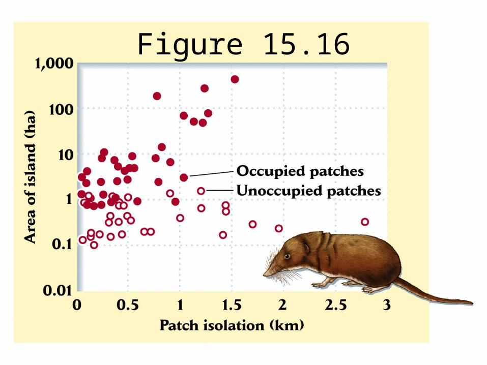
Figure 15.16

Figure 15.17a

Figure 15.17b

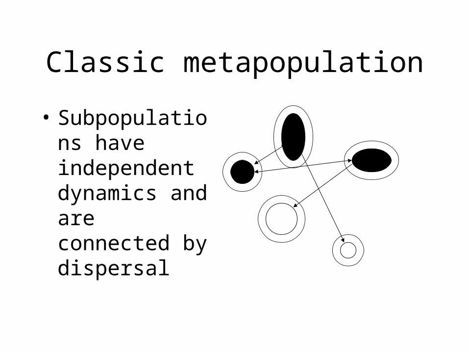
Classic metapopulation

• Subpopulations have independent dynamics and are connected by dispersal

Mainland-Island metapopulation

• R. MacArthur and E.O. Wilson 1967

• 1 area persists indefinitely and provides colonists to other areas that go extinct

Source-Sink metapopulation

• R. Pulliam 1988• In sources,

R>1• In sinks, R<1• Sinks persist

because they are resupplied with individuals from sources

Source-Sink metapopulation

• Do all subpopulations with high have high density?

• Which would contribute more to conservation, high or high density?